APPLYING SYNTHETIC APERTURE, CODED EXCITATION, AND

TISSUE HARMONIC IMAGING TECHNIQUES TO ALLOW

ULTRASOUND IMAGING WITH A VIRTUAL SOURCE

BY

ROBYN T. UMEKI

THESIS

Submitted in partial fulfillment of the requirements

for the degree of Master of Science in Electrical and Computer Engineering

in the Graduate College of the

University of Illinois at Urbana-Champaign, 2011

Urbana, Illinois

Adviser:

Assistant Professor Michael Oelze

ii

ABSTRACT

A focused transducer will concentrate its signal energy at its focus, producing a clear

image of objects at that depth. However, spatial resolution and signal strength deteriorate away

from the transducer’s focus. Therefore, having only one focal length places a great restriction on

ultrasound imaging, especially with a single-element transducer. To extend the region of focus,

three techniques were examined. The first was the synthetic aperture focusing technique (SAFT),

a well-studied method that allows focus at every distance instead of just one distance. Using this

method, lateral resolution is restored and signal-to-noise ratio (SNR) is increased due to the

compounding of several scan lines. SAFT was combined with a virtual source technique to

further extend the region of focus. The second technique examined was coded excitation, a

means of improving SNR while maintaining the axial resolution. The third technique was tissue

harmonic imaging, which produces a narrower beamwidth and reduced sidelobes, and therefore

can improve spatial resolution and contrast of images.

Each technique is individually known to improve ultrasound image qualities, with its own

strengths and drawbacks. This study combines all three. In the final stage of this study using the

virtual source technique, harmonic imaging was implemented using coded excitation beyond the

transducer focus. Because of the low signal strength received under the synthetic aperture

technique, harmonic imaging has never been attempted using SAFT and a virtual source. There

has been no previous research to determine whether the techniques will build on each other or

detract from each other.

This study included simulations and experiments with the techniques applied to a single

scatterer, as well as experiments with a tissue-mimicking phantom. Implementing coded

excitation with SAFT led to a final SNR higher than was observed when applying SAFT alone.

Although coding helped to increase SNR, the sidelobes became much more visible.

Additionally, it was found that synthetic aperture was not a linear process and could cause

distortion when the transmitted pulse is very long. This problem was eliminated when time

compression was applied before SAFT. When applying tissue harmonic imaging, the sidelobes

were less prominent than before. However, the speckle increased and the SNR decreased, likely

due to the decreased signal strength of the transducer at the harmonic frequencies.

iii

This study has shown that synthetic aperture with a virtual source, coded excitation, and

tissue harmonic imaging can be combined to image beyond the focal length of a transducer.

However, there was no research on the maximum depth at which the technique can be practical.

Additionally, this study did not test the effectiveness of the techniques when applied to real

tissue.

iv

TABLE OF CONTENTS

CHAPTER 1: INTRODUCTION................................................................................................1

CHAPTER 2: BACKGROUND INFORMATION......................................................................4

CHAPTER 3: METHODS ........................................................................................................17

CHAPTER 4: RESULTS ..........................................................................................................27

CHAPTER 5: CONCLUSION ..................................................................................................39

REFERENCES .........................................................................................................................41

1

CHAPTER 1: INTRODUCTION

1.1. Motivation

Ultrasound can serve many purposes, but the best-known use is medical imaging. Ultrasound

imaging is based on reflection and scattering that occurs when a wave meets a boundary between

different media (e.g. two different tissues). By recording the time series echo and converting to a

range through the sound speed, the locations of the boundaries can be imaged. Ultrasound

images are constructed by combining scan lines of backscattered echoes separated by some

lateral distance. The lateral separation is related to the beamwidth of the ultrasonic imaging

device.

There are several important qualities desired in an image. Three characteristics that can

be quantified are signal-to-noise ratio (SNR), contrast resolution (CR), and spatial resolution.

SNR is an indication of the signal’s strength; a higher SNR makes it easier to see details that

would be obscured by noise. CR describes how well the area of interest contrasts from

background. With better contrast, it is easier to detect changes in intensity between tissues or

irregularities. Spatial resolution is the ability to distinguish between nearby points of interest.

With poor spatial resolution, two separate objects within the field of view may appear to be one

larger object. A combination of these three qualities is necessary to be able to produce a good

ultrasound image. However, these quantities may vary in different parts of the image. Overall

image quality can be optimized by improving SNR, CR, or spatial resolution.

Lateral resolution and SNR deteriorate away from the transducer’s focal length.

Therefore, imaging at distances too far away from the focal length will have poor lateral

resolution and signal strength. Poor spatial resolution and SNR will also cause a decrease in CR.

Therefore, having only one focal length places a great restriction on ultrasound imaging.

One way to expand the region of focus for imaging is to use synthetic aperture techniques

with a virtual source, which is a well-studied technique used to restore lateral resolution and

increase SNR when imaging beyond the transducer’s focal length [1], [2]. In effect, the focus of

a transducer acts like a point source without a focus. The data can then be processed so that the

focus is translated to every distance instead of just one distance.

The signals outside the focus are generally lower than signals within the depth of field.

As a result, virtual source methods can suffer from low SNR and may not have sufficient SNR to

2

provide good images. One means of improving the SNR while maintaining the spatial resolution

is to use coded excitation [3], [4]. Therefore, it is hypothesized in this study that coded excitation

techniques can be combined with virtual source techniques to improve imaging using a virtual

source.

In addition to using coded excitation and virtual source techniques, tissue harmonic

imaging may also be combined with virtual source and coded excitation to further improve

characteristics of the imaging system. Harmonic imaging is a technique that works with the

harmonics of the pulse that are generated due to nonlinear properties of the medium. Harmonic

imaging techniques have the advantages of higher frequencies but reduced attenuation on the

forward propagation, better lateral resolution, and reduced sidelobes compared to conventional

imaging techniques [5]. Therefore, harmonic imaging can improve spatial resolution and

improve contrast of images. However, because of the low SNR from the virtual source

technique, harmonic imaging has never been attempted using a virtual source.

1.2. Goals

All of the above techniques are known to improve ultrasound image qualities, with their own

strengths and drawbacks. However, the techniques have not been combined. There has been no

previous research to determine whether the techniques will build on each other (i.e., mitigate

some of the negative tradeoffs associated with each technique) or detract from each other.

The goal of this study is to determine the effects of combining synthetic aperture, virtual

source, coded excitation, and harmonic imaging techniques in ultrasound imaging. Each

individual technique will be studied, as well as combinations of them. The study includes

simulations and experiments of the techniques applied to a single scatterer and experiments with

a tissue-mimicking phantom. The results from the different techniques will be compared both

visually and quantitatively.

1.3. Organization

The following chapters will explain more details about this research. Chapter 2 provides

background information on ultrasound imaging and the different techniques being studied.

Chapter 3 describes the approach of the study and details the experimental setup, and Chapter 4

3

presents the results of the experimentation. Chapter 5 concludes the thesis with discussion of the

results and suggestions for future work.

4

CHAPTER 2: BACKGROUND INFORMATION

2.1. Ultrasound Imaging and Transducers

Ultrasonic waves are defined as acoustic pressure waves oscillating at frequencies above 20 kHz,

the approximate upper limit of human hearing. The properties of an ultrasonic wave are

dependent upon the medium in which it is traveling. The medium’s properties define its

characteristic impedance. At the boundary between two tissues, there is an impedance mismatch.

When a wave is incident upon such a boundary, part of the energy is transmitted and part of it is

reflected and/or scattered. These reflections are exploited in ultrasound imaging. A transmitted

wave will encounter different media and return reflection information.

If the sound speed can be assumed, the time between transmission and reception of the

echo and the strength of the echo reveal the distance and level of mismatch of an object in view.

However, waves are not transmitted without loss. Each tissue will cause a certain amount of

attenuation to a pressure wave versus distance. The level of attenuation depends on the tissue and

the frequency of the wave; higher frequencies generally suffer higher attenuation. Due to

attenuation, the signal-to noise ratio (SNR) decreases away from the transducer. Additionally, a

speckle pattern is caused by sub-resolution scatterers that are inherent to the tissue and can

detract from the image when it is strong.

In ultrasound imaging, transducers are used to generate pressure waves. Currently, most

transducers use piezoelectric material to convert electrical energy to mechanical energy, and vice

versa. The piezoelectric material’s behavior depends on a number of factors, including the

material’s properties and the pressure or voltage applied to it. It will have a resonant frequency

of oscillation, which is reflected in its impulse response. Other frequencies will not be

transmitted and received as strongly.

To focus the pressure wave, the transducer can be designed with different shapes, as with

an optical lens. For a concave focused transducer, the transducer’s level of focus is quantified by

its focal number:

D

Ff =# , (2.1)

5

where f# is the focal number, F is the focal length, and D is the transducer’s diameter. A highly

focused transducer will have a low focal number, while a less focused transducer will have a

higher focal number.

A highly focused transducer creates more pressure at its focus than an unfocused or

weakly focused transducer. Therefore, it has a higher SNR at the focus than a less focused

transducer would have. Furthermore, because the pressure is more concentrated at the focus,

there is a rapid decrease in the pressure amplitude away from the source. The beamwidth at the

focus is smaller than an unfocused source, allowing better lateral resolution. However, with

focusing the depth of field, or range of imaging, is also reduced, making it harder to image

objects outside the depth of field, limiting the axial range at which imaging can occur.

When a pulse is emitted from a transducer, the pulse propagates away from the

transducer and into the surrounding medium. However, because of the shape and size of the

transducer aperture, the energy of the pulse will be confined to small defined regions called the

beam pattern of the transducer. As the pulse propagates into the medium, within the beam of the

transducer, the pulse is reflected or scattered back towards the source. The beam pattern allows a

smaller region laterally to be interrogated with the source; hence, the lateral resolution is

dependent on the beamwidth. The reflected or scattered pulses that return to the source sum

together at the source in time and create a complex waveform in time. This signal is called a

backscattered scan line. By detecting the envelope of the scan line signal and calculating the

range from the assumed sound speed, an A-mode line is formed relating the strength of the echo

signal to a range. The transducer can then be translated laterally to acquire another scan line from

targets located within the beam.

When several parallel scans combine to form an image, it is called a B-mode scan. A B-

mode image is produced by receiving and processing the parallel echoes. To produce each scan

line, the transducer communicates the pressure received along its aperture for each time sample.

Then, the scan line is envelope detected via a Hilbert transform. The envelope magnitude is

converted to a dB scale. The scan lines are aligned with each other and plotted as an image, so

that the intensity of the echoes correlates with the brightness of the image.

6

2.2. Synthetic Aperture Theory

When an object is scanned using B-mode imaging, lateral resolution is optimal at the

transducer’s focal length. Regions outside of the focus return lower SNR and worse spatial

resolution than at the focus. One way to put the whole field in focus is to apply synthetic aperture

focusing technique (SAFT).

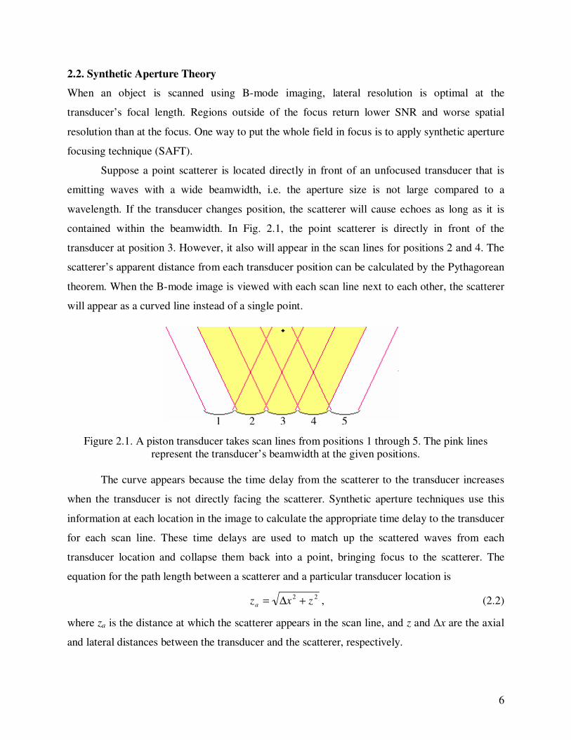
Suppose a point scatterer is located directly in front of an unfocused transducer that is

emitting waves with a wide beamwidth, i.e. the aperture size is not large compared to a

wavelength. If the transducer changes position, the scatterer will cause echoes as long as it is

contained within the beamwidth. In Fig. 2.1, the point scatterer is directly in front of the

transducer at position 3. However, it also will appear in the scan lines for positions 2 and 4. The

scatterer’s apparent distance from each transducer position can be calculated by the Pythagorean

theorem. When the B-mode image is viewed with each scan line next to each other, the scatterer

will appear as a curved line instead of a single point.

Figure 2.1. A piston transducer takes scan lines from positions 1 through 5. The pink lines

represent the transducer’s beamwidth at the given positions.

The curve appears because the time delay from the scatterer to the transducer increases

when the transducer is not directly facing the scatterer. Synthetic aperture techniques use this

information at each location in the image to calculate the appropriate time delay to the transducer

for each scan line. These time delays are used to match up the scattered waves from each

transducer location and collapse them back into a point, bringing focus to the scatterer. The

equation for the path length between a scatterer and a particular transducer location is

22

zxza +∆= , (2.2)

where za is the distance at which the scatterer appears in the scan line, and z and ∆x are the axial

and lateral distances between the transducer and the scatterer, respectively.

1 2 3 4 5

7

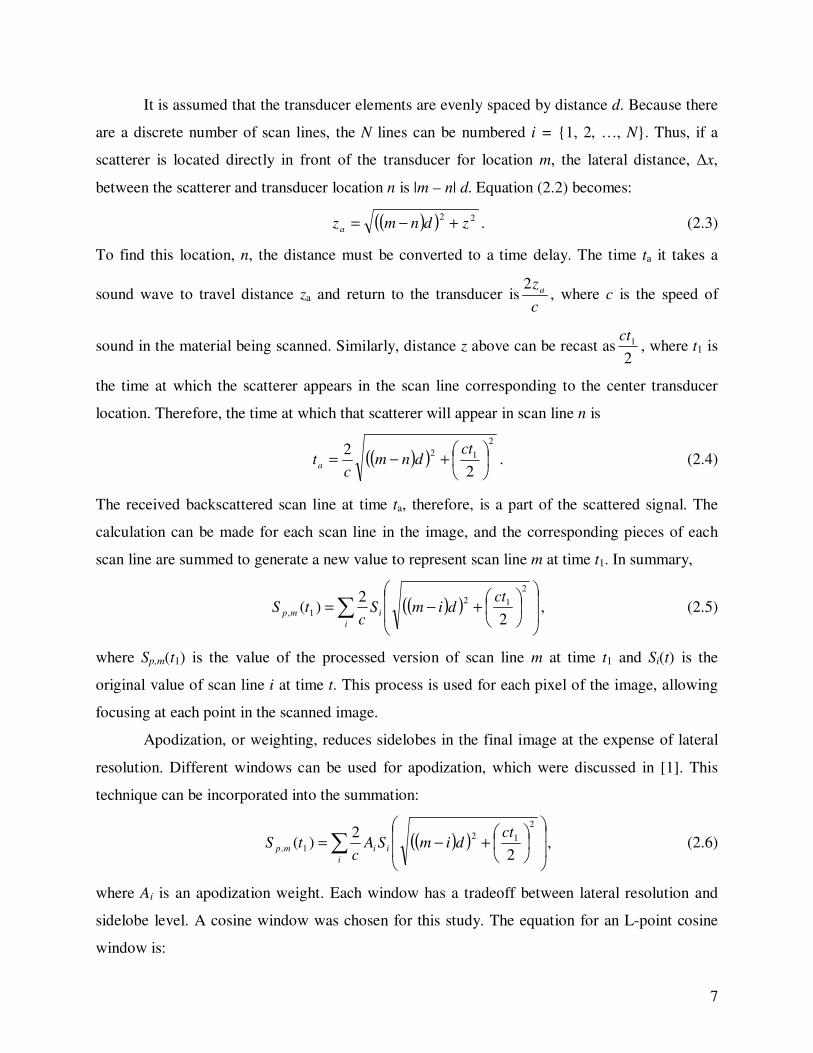
It is assumed that the transducer elements are evenly spaced by distance d. Because there

are a discrete number of scan lines, the N lines can be numbered i = {1, 2, …, N}. Thus, if a

scatterer is located directly in front of the transducer for location m, the lateral distance, ∆x,

between the scatterer and transducer location n is |m – n| d. Equation (2.2) becomes:

( )( ) 22zdnmza +−= . (2.3)

To find this location, n, the distance must be converted to a time delay. The time ta it takes a

sound wave to travel distance za and return to the transducer isc

za

2, where c is the speed of

sound in the material being scanned. Similarly, distance z above can be recast as2

1ct, where t1 is

the time at which the scatterer appears in the scan line corresponding to the center transducer

location. Therefore, the time at which that scatterer will appear in scan line n is

( )( )2

12

2

2

+−=

ctdnm

cta . (2.4)

The received backscattered scan line at time ta, therefore, is a part of the scattered signal. The

calculation can be made for each scan line in the image, and the corresponding pieces of each

scan line are summed to generate a new value to represent scan line m at time t1. In summary,

( )( )∑

+−=

i

imp

ctdimS

ctS

2

12

1,2

2)( , (2.5)

where Sp,m(t1) is the value of the processed version of scan line m at time t1 and Si(t) is the

original value of scan line i at time t. This process is used for each pixel of the image, allowing

focusing at each point in the scanned image.

Apodization, or weighting, reduces sidelobes in the final image at the expense of lateral

resolution. Different windows can be used for apodization, which were discussed in [1]. This

technique can be incorporated into the summation:

( )( )∑

+−=

i

iimp

ctdimSA

ctS

2

12

1,2

2)( , (2.6)

where Ai is an apodization weight. Each window has a tradeoff between lateral resolution and

sidelobe level. A cosine window was chosen for this study. The equation for an L-point cosine

window is:

8

−

−−

2

12

1

2cos

L

Ll

π, (2.7)

where n is the index { }1,...,2,1,0 −∈ Ll . For this application, L can be set to the number of scan

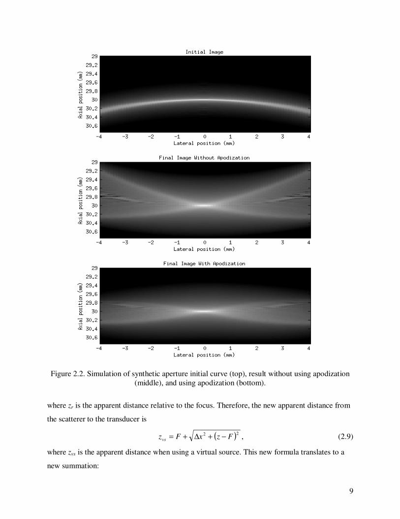
lines being summed. An example of the improvement when applying apodization is shown in

Fig. 2.2. Without apodization, the scatterer location was clearly visible, but the sidelobes

spanned a large area. When apodization was applied, the scatterer appeared wider in the lateral

direction, but the sidelobes were constrained to a smaller area.

The summation process is repeated for each axial position in the scan line, and for each

scan line. Therefore, synthetic aperture can be applied at all distances within the scan, allowing

focus at all distances instead of just one focal length. In this scenario, a wide beam spread is ideal

because it allows more scan lines to be summed, increasing SNR and reducing sidelobes.

However, the beamwidth of an unfocused transducer is primarily dependent on the size of the

transducer, reducing the applications for synthetic aperture alone. By having a smaller aperture

size, the beamwidth spreads out more but also at the expense of a reduced acoustic output power.

2.3. Virtual Source Theory

The virtual source technique is an extension of synthetic aperture. Instead of imaging areas close

to the transducer, a virtual source helps image areas beyond the transducer’s focal length. This

technique is based on the idea that the transducer will produce pressure waves that converge

towards the focus, and diverge from there. It is assumed that within a certain beamwidth angleφ ,

the waves emerge from the focal point spherically, as if the waves are being produced from a

spherical source at this location. Thus, the focus of the transducer becomes a virtual source, as

shown in Fig. 2.3. Because the waves are spreading away from the virtual source, this model

allows easy application of synthetic aperture techniques to areas beyond the virtual source. Also,

by applying the SAFT technique to the points beyond the focus, the SNR of the resulting spatial

compressed signals will be increased.

To account for the shift from calculating distance in reference to the virtual source

instead of the transducer, the equation for path length becomes

( )22 Fzxz r −+∆= , (2.8)

9

Figure 2.2. Simulation of synthetic aperture initial curve (top), result without using apodization

(middle), and using apodization (bottom).

where zr is the apparent distance relative to the focus. Therefore, the new apparent distance from

the scatterer to the transducer is

( )22 FzxFzvs −+∆+= , (2.9)

where zvs is the apparent distance when using a virtual source. This new formula translates to a

new summation:

10

Figure 2.3. A focused transducer takes scan lines from positions 1 through 5. The pink lines

represent the transducer’s beamwidth beyond the virtual source at the given positions.

( )( )∑

−+−+=

i

iimvs Fct

dimFSAc

tS

2

12

1,2

2)( , (2.10)

where Svs,m(t1) is the resulting value of scan line m at time t1. Additionally, i must be restricted to

the scan lines contained within the beamwidth. Using simple geometry, the half-angle 2

φ at

which the wave spreads from the virtual source is approximately

= −

F

D

2tan

2

1φ. (2.11)

Therefore, the beamwidth limit at distance z is

#22

tanf

zz =

φ. (2.12)

As a result, the scatterer should not appear in a scan line unless#2 f

zx <∆ . In terms of the time-

series echoes, this relationship becomes#

1

4 f

ctx <∆ , or

#

1

4 f

ctdim <− . (2.13)

In this scenario, the wide beam desired in synthetic aperture will be best achieved by a

highly focused transducer because the beamwidth at the focus is proportional to the wavelength

times the f-number. A highly focused transducer will project a beam that sharply converges at

the focus and diverges at a wide angle, so that a distant scatterer will appear in multiple scan

1 2 3 4 5

φ

11

lines. Because the signals being summed are from outside the focal depth, the original received

signals can have low SNR. By summing the contributions from several scan lines, the SNR of

the subsequent focused image will be improved. However, low SNR continues to be an issue

with virtual source imaging techniques.

2.4. Coded Excitation Theory

One way to overcome the limitations of the low SNR in the virtual source imaging technique is

too use coded excitation and pulse compression. Coded excitation is a method to improve SNR

by transmitting a signal with certain known and advantageous characteristics. The received

signal can then be processed to improve the quality of the data for imaging. This effect is

accomplished by applying an excitation signal f(t) of significantly longer duration than the

impulse response of the source and whose autocorrelation Rf(t) is approximately a delta function.

When it is applied to a transducer with a pulse-echo impulse response h(t), the received

waveform is

)(*)()( thtftp = . (2.14)

When the pressure wave is returned to the transducer, the received signal can then be

decoded or compressed using f(t). The compression step takes the longer duration signal and

compresses it so that the axial resolution is approximately that of the impulse response of the

system. The easiest method of compression is accomplished by cross correlation of the received

signal with the excitation signal:

)()()( tptftq ⊗= . (2.15)

Assuming f(t) and h(t) are real signals, this equation can be reduced to

)(*)()( tRthtq f= . (2.16)

For )()( ttR f δ= , the equation reduces to

)()( thtq = . (2.17)

The prolonged excitation signal has multiple effects. The length causes p(t) itself to have

poor axial resolution compared to the image resulting from an impulse excitation. However, it

allows more energy to be applied, without increasing the pressure amplitude. With the step of

compression, axial resolution is restored in q(t), and the increased energy allows an increase in

SNR.

12

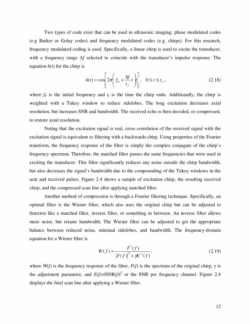
Two types of code exist that can be used in ultrasonic imaging: phase modulated codes

(e.g Barker or Golay codes) and frequency modulated codes (e.g. chirps). For this research,

frequency modulated coding is used. Specifically, a linear chirp is used to excite the transducer,

with a frequency range ∆f selected to coincide with the transducer’s impulse response. The

equation h(t) for the chirp is

∆+= tt

t

ffth

f

02cos)( π , ftt ≤≤0 , (2.18)

where f0 is the initial frequency and tf is the time the chirp ends. Additionally, the chirp is

weighted with a Tukey window to reduce sidelobes. The long excitation decreases axial

resolution, but increases SNR and bandwidth. The received echo is then decoded, or compressed,

to restore axial resolution.

Noting that the excitation signal is real, cross correlation of the received signal with the

excitation signal is equivalent to filtering with a backwards chirp. Using properties of the Fourier

transform, the frequency response of the filter is simply the complex conjugate of the chirp’s

frequency spectrum. Therefore, the matched filter passes the same frequencies that were used in

exciting the transducer. This filter significantly reduces any noise outside the chirp bandwidth,

but also decreases the signal’s bandwidth due to the compounding of the Tukey windows in the

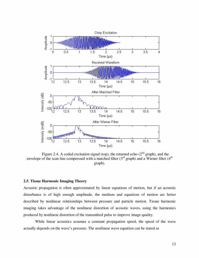
sent and received pulses. Figure 2.4 shows a sample of excitation chirp, the resulting received

chirp, and the compressed scan line after applying matched filter.

Another method of compression is through a Fourier filtering technique. Specifically, an

optimal filter is the Wiener filter, which also uses the original chirp but can be adjusted to

function like a matched filter, inverse filter, or something in between. An inverse filter allows

more noise, but retains bandwidth. The Wiener filter can be adjusted to get the appropriate

balance between reduced noise, minimal sidelobes, and bandwidth. The frequency-domain

equation for a Wiener filter is

)()(

)()(

12

*

fEfF

fFfW

−+=

γ, (2.19)

where W(f) is the frequency response of the filter, F(f) is the spectrum of the original chirp, γ is

the adjustment parameter, and E(f)=|SNR(f)|2 or the SNR per frequency channel. Figure 2.4

displays the final scan line after applying a Wiener filter.

13

Figure 2.4. A coded excitation signal (top), the returned echo (2nd

graph), and the

envelope of the scan line compressed with a matched filter (3rd

graph) and a Wiener filter (4th

graph).

2.5. Tissue Harmonic Imaging Theory

Acoustic propagation is often approximated by linear equations of motion, but if an acoustic

disturbance is of high enough amplitude, the medium and equations of motion are better

described by nonlinear relationships between pressure and particle motion. Tissue harmonic

imaging takes advantage of the nonlinear distortion of acoustic waves, using the harmonics

produced by nonlinear distortion of the transmitted pulse to improve image quality.

While linear acoustics assumes a constant propagation speed, the speed of the wave

actually depends on the wave’s pressure. The nonlinear wave equation can be stated as

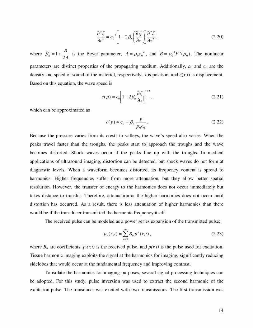
14

2

22

02

2

21xx

ct

n∂

∂

∂

∂−=

∂

∂ ξξβ

ξ, (2.20)

where A

Bn

21+=β is the Beyer parameter,

2

00cA ρ= , and )('' 0

2

0 ρρ PB = . The nonlinear

parameters are distinct properties of the propagating medium. Additionally, ρ0 and c0 are the

density and speed of sound of the material, respectively, x is position, and ξ(x,t) is displacement.

Based on this equation, the wave speed is

2/1

0 21)(

∂

∂−=

xcpc n

ξβ , (2.21)

which can be approximated as

00

0)(c

pcpc n

ρβ+≈ . (2.22)

Because the pressure varies from its crests to valleys, the wave’s speed also varies. When the

peaks travel faster than the troughs, the peaks start to approach the troughs and the wave

becomes distorted. Shock waves occur if the peaks line up with the troughs. In medical

applications of ultrasound imaging, distortion can be detected, but shock waves do not form at

diagnostic levels. When a waveform becomes distorted, its frequency content is spread to

harmonics. Higher frequencies suffer from more attenuation, but they allow better spatial

resolution. However, the transfer of energy to the harmonics does not occur immediately but

takes distance to transfer. Therefore, attenuation at the higher harmonics does not occur until

distortion has occurred. As a result, there is less attenuation of higher harmonics than there

would be if the transducer transmitted the harmonic frequency itself.

The received pulse can be modeled as a power series expansion of the transmitted pulse:

∑∞

=

=0

),(),(n

n

nr trpBtrp , (2.23)

where Bn are coefficients, pr(r,t) is the received pulse, and p(r,t) is the pulse used for excitation.

Tissue harmonic imaging exploits the signal at the harmonics for imaging, significantly reducing

sidelobes that would occur at the fundamental frequency and improving contrast.

To isolate the harmonics for imaging purposes, several signal processing techniques can

be adopted. For this study, pulse inversion was used to extract the second harmonic of the

excitation pulse. The transducer was excited with two transmissions. The first transmission was

15

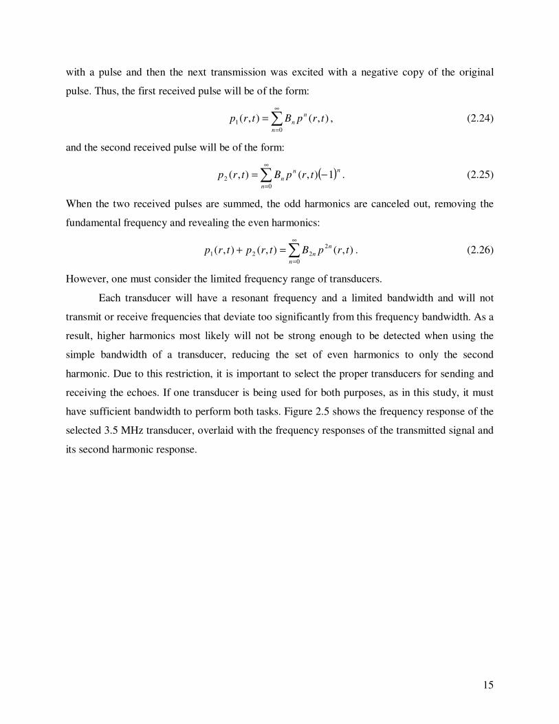
with a pulse and then the next transmission was excited with a negative copy of the original

pulse. Thus, the first received pulse will be of the form:

∑∞

=

=0

1 ),(),(n

n

n trpBtrp , (2.24)

and the second received pulse will be of the form:

( )n

n

n

n trpBtrp 1),(),(0

2 −=∑∞

=

. (2.25)

When the two received pulses are summed, the odd harmonics are canceled out, removing the

fundamental frequency and revealing the even harmonics:

∑∞

=

=+0

2

221 ),(),(),(n

n

n trpBtrptrp . (2.26)

However, one must consider the limited frequency range of transducers.

Each transducer will have a resonant frequency and a limited bandwidth and will not

transmit or receive frequencies that deviate too significantly from this frequency bandwidth. As a

result, higher harmonics most likely will not be strong enough to be detected when using the

simple bandwidth of a transducer, reducing the set of even harmonics to only the second

harmonic. Due to this restriction, it is important to select the proper transducers for sending and

receiving the echoes. If one transducer is being used for both purposes, as in this study, it must

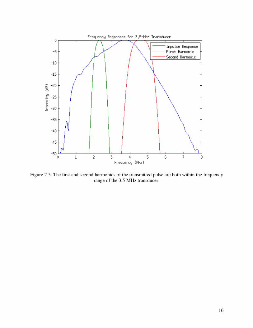
have sufficient bandwidth to perform both tasks. Figure 2.5 shows the frequency response of the

selected 3.5 MHz transducer, overlaid with the frequency responses of the transmitted signal and

its second harmonic response.

16

Figure 2.5. The first and second harmonics of the transmitted pulse are both within the frequency

range of the 3.5 MHz transducer.

17

CHAPTER 3: METHODS

3.1. Simulations

Simulations allow the prediction of outcomes without the cost in time and equipment and the

variability of real data collection. The preliminary results help judge the effectiveness of a

technique before performing a full experiment, and help ensure it is being implemented

correctly. In this study, Matlab (The Mathworks Inc., Natick, MA) programs were developed to

perform all of the techniques being studied, and Field II [6], [7] was used within Matlab to

produce simulated data. Field II uses several transducer parameters to analytically calculate a

response. The effects of SAFT and coded excitation were simulated before collecting data in a

laboratory.

3.1.1. Synthetic aperture alone

The first step was to develop a Matlab program using Field II to simulate the imaging of

a point target. The resulting image could then be used in the development of code for performing

synthetic aperture. The first version of this program used a 250 MHz sampling rate and a flat

piston transducer with 0.24 mm radius. For simplicity, the transducer impulse response was a

delta impulse, the speed of sound was set to 1500 m/s, and there was no attenuation or noise. The

point scatterer was located 30 mm away from the transducer, and 100 scan lines were simulated

at 0.5 mm increments. A distance vector was calculated to correspond to the received scans.

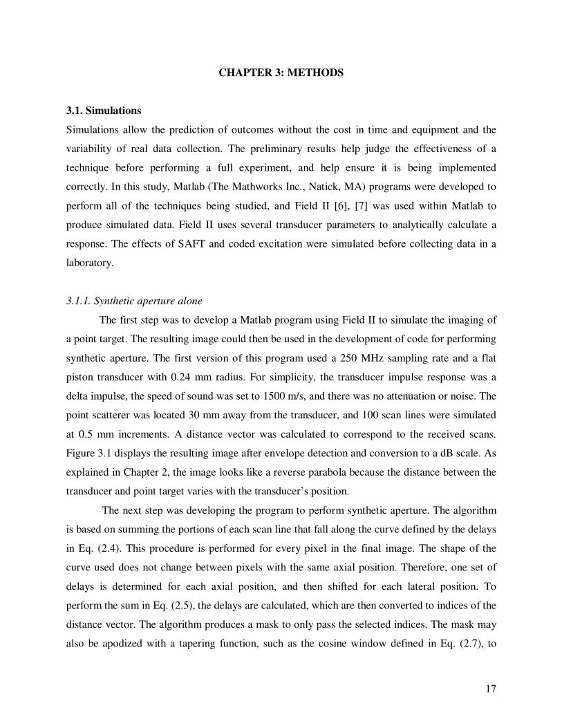
Figure 3.1 displays the resulting image after envelope detection and conversion to a dB scale. As

explained in Chapter 2, the image looks like a reverse parabola because the distance between the

transducer and point target varies with the transducer’s position.

The next step was developing the program to perform synthetic aperture. The algorithm

is based on summing the portions of each scan line that fall along the curve defined by the delays

in Eq. (2.4). This procedure is performed for every pixel in the final image. The shape of the

curve used does not change between pixels with the same axial position. Therefore, one set of

delays is determined for each axial position, and then shifted for each lateral position. To

perform the sum in Eq. (2.5), the delays are calculated, which are then converted to indices of the

distance vector. The algorithm produces a mask to only pass the selected indices. The mask may

also be apodized with a tapering function, such as the cosine window defined in Eq. (2.7), to

18

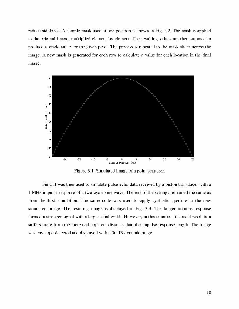
reduce sidelobes. A sample mask used at one position is shown in Fig. 3.2. The mask is applied

to the original image, multiplied element by element. The resulting values are then summed to

produce a single value for the given pixel. The process is repeated as the mask slides across the

image. A new mask is generated for each row to calculate a value for each location in the final

image.

Figure 3.1. Simulated image of a point scatterer.

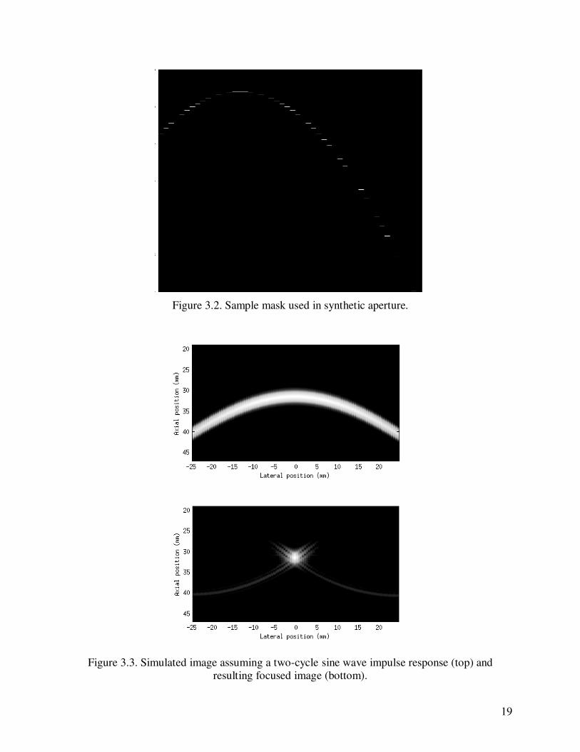
Field II was then used to simulate pulse-echo data received by a piston transducer with a

1 MHz impulse response of a two-cycle sine wave. The rest of the settings remained the same as

from the first simulation. The same code was used to apply synthetic aperture to the new

simulated image. The resulting image is displayed in Fig. 3.3. The longer impulse response

formed a stronger signal with a larger axial width. However, in this situation, the axial resolution

suffers more from the increased apparent distance than the impulse response length. The image

was envelope-detected and displayed with a 50 dB dynamic range.

19

Figure 3.2. Sample mask used in synthetic aperture.

Figure 3.3. Simulated image assuming a two-cycle sine wave impulse response (top) and

resulting focused image (bottom).

20

3.1.2. Synthetic aperture with a virtual source

After developing the synthetic aperture simulation, virtual source techniques were added

to the simulations. There were two primary changes required to incorporate the virtual source

into SAFT. The first was adjusting the synthetic aperture curve to account for the position of the

virtual source. As shown in Eq. (2.9), the virtual source was located at the focal point, so the

distance calculations were made relative to the focal point instead of the transducer, and then

added to the focal length. These changes were incorporated into the same delay calculations that

were used previously when performing synthetic aperture based on the actual transducer

element.

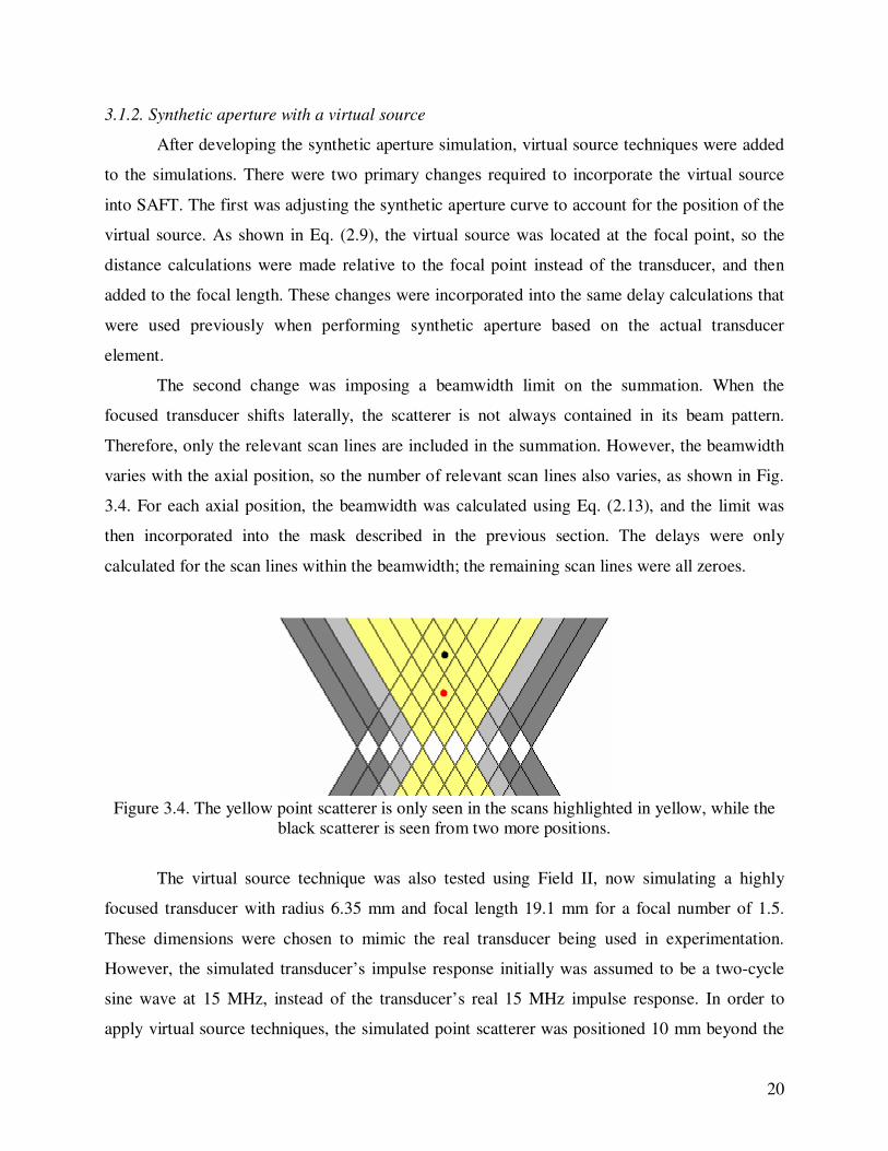
The second change was imposing a beamwidth limit on the summation. When the

focused transducer shifts laterally, the scatterer is not always contained in its beam pattern.

Therefore, only the relevant scan lines are included in the summation. However, the beamwidth

varies with the axial position, so the number of relevant scan lines also varies, as shown in Fig.

3.4. For each axial position, the beamwidth was calculated using Eq. (2.13), and the limit was

then incorporated into the mask described in the previous section. The delays were only

calculated for the scan lines within the beamwidth; the remaining scan lines were all zeroes.

Figure 3.4. The yellow point scatterer is only seen in the scans highlighted in yellow, while the

black scatterer is seen from two more positions.

The virtual source technique was also tested using Field II, now simulating a highly

focused transducer with radius 6.35 mm and focal length 19.1 mm for a focal number of 1.5.

These dimensions were chosen to mimic the real transducer being used in experimentation.

However, the simulated transducer’s impulse response initially was assumed to be a two-cycle

sine wave at 15 MHz, instead of the transducer’s real 15 MHz impulse response. In order to

apply virtual source techniques, the simulated point scatterer was positioned 10 mm beyond the

21

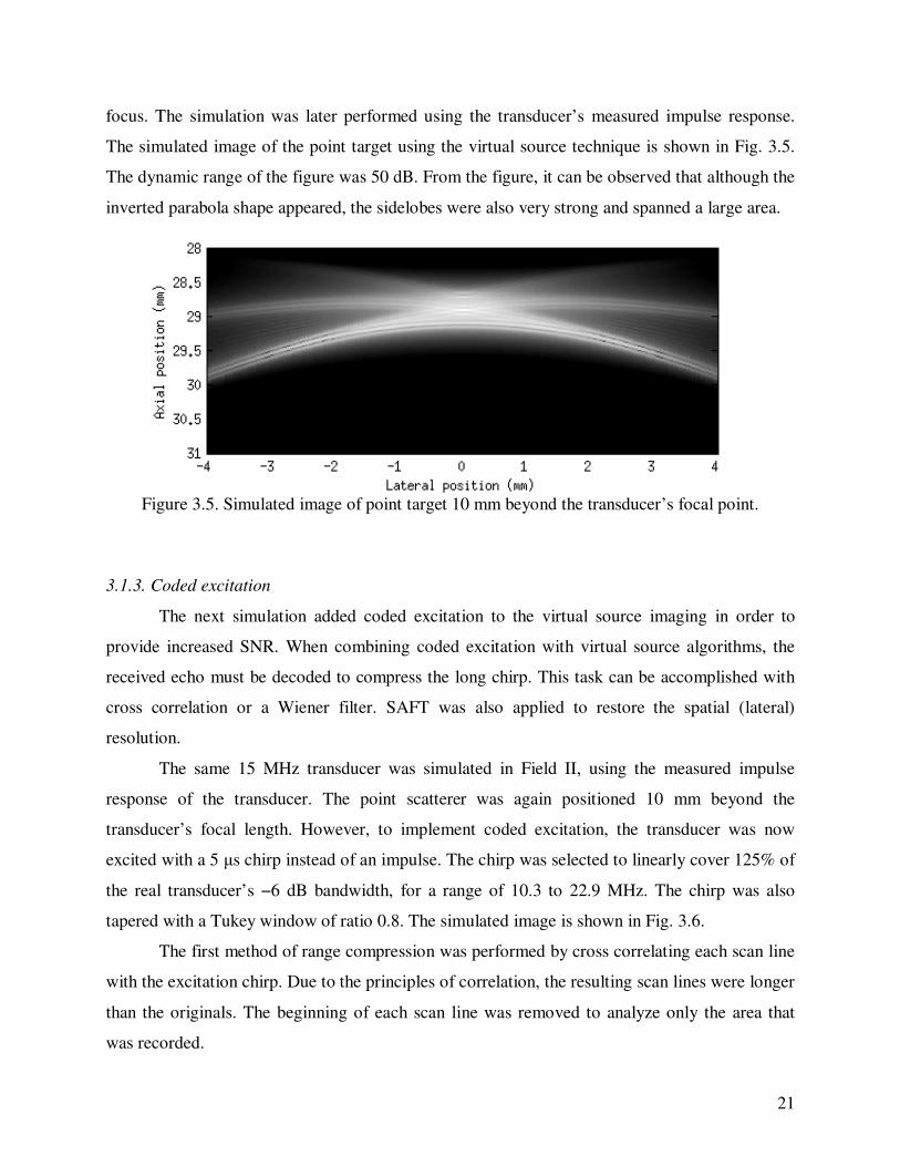
focus. The simulation was later performed using the transducer’s measured impulse response.

The simulated image of the point target using the virtual source technique is shown in Fig. 3.5.

The dynamic range of the figure was 50 dB. From the figure, it can be observed that although the

inverted parabola shape appeared, the sidelobes were also very strong and spanned a large area.

Figure 3.5. Simulated image of point target 10 mm beyond the transducer’s focal point.

3.1.3. Coded excitation

The next simulation added coded excitation to the virtual source imaging in order to

provide increased SNR. When combining coded excitation with virtual source algorithms, the

received echo must be decoded to compress the long chirp. This task can be accomplished with

cross correlation or a Wiener filter. SAFT was also applied to restore the spatial (lateral)

resolution.

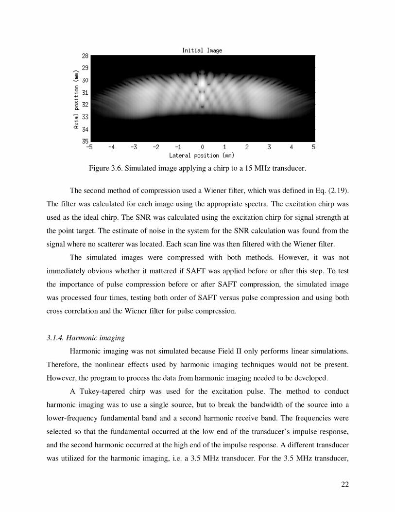
The same 15 MHz transducer was simulated in Field II, using the measured impulse

response of the transducer. The point scatterer was again positioned 10 mm beyond the

transducer’s focal length. However, to implement coded excitation, the transducer was now

excited with a 5 µs chirp instead of an impulse. The chirp was selected to linearly cover 125% of

the real transducer’s −6 dB bandwidth, for a range of 10.3 to 22.9 MHz. The chirp was also

tapered with a Tukey window of ratio 0.8. The simulated image is shown in Fig. 3.6.

The first method of range compression was performed by cross correlating each scan line

with the excitation chirp. Due to the principles of correlation, the resulting scan lines were longer

than the originals. The beginning of each scan line was removed to analyze only the area that

was recorded.

22

Figure 3.6. Simulated image applying a chirp to a 15 MHz transducer.

The second method of compression used a Wiener filter, which was defined in Eq. (2.19).

The filter was calculated for each image using the appropriate spectra. The excitation chirp was

used as the ideal chirp. The SNR was calculated using the excitation chirp for signal strength at

the point target. The estimate of noise in the system for the SNR calculation was found from the

signal where no scatterer was located. Each scan line was then filtered with the Wiener filter.

The simulated images were compressed with both methods. However, it was not

immediately obvious whether it mattered if SAFT was applied before or after this step. To test

the importance of pulse compression before or after SAFT compression, the simulated image

was processed four times, testing both order of SAFT versus pulse compression and using both

cross correlation and the Wiener filter for pulse compression.

3.1.4. Harmonic imaging

Harmonic imaging was not simulated because Field II only performs linear simulations.

Therefore, the nonlinear effects used by harmonic imaging techniques would not be present.

However, the program to process the data from harmonic imaging needed to be developed.

A Tukey-tapered chirp was used for the excitation pulse. The method to conduct

harmonic imaging was to use a single source, but to break the bandwidth of the source into a

lower-frequency fundamental band and a second harmonic receive band. The frequencies were

selected so that the fundamental occurred at the low end of the transducer’s impulse response,

and the second harmonic occurred at the high end of the impulse response. A different transducer

was utilized for the harmonic imaging, i.e. a 3.5 MHz transducer. For the 3.5 MHz transducer,

23

the bandwidth ranged from 1.8 to 2.8 MHz (the fundamental bandwidth), so that the second

harmonic bandwidth would occur from 3.6 to 5.6 MHz. These ranges helped ensure the

transducer would have the bandwidth to both send and receive the desired frequencies. The

transducer was assumed to have a wide enough bandwidth to handle transmitting and receiving

both the first and the second harmonics. Incorporating coded excitation, the excitation signal was

assumed to be a chirp at a range of frequencies along the low end of the transducer’s bandwidth.

Pulse inversion was used to extract the second harmonic, so two chirps were simulated to

be transmitted by the transducer. The first and second chirps were assumed to be 180o out of

phase so that the sum of the two received signals would remove the fundamental frequency

range. The second harmonic would occur at twice the frequencies of the original chirps and be

enhanced using the pulse inversion technique. After the pulse inversion technique was invoked, a

Wiener filter was chosen to perform time compression on the chirp’s second harmonic.

3.2. Experimental Setup

3.2.1. Synthetic aperture with a virtual source

After performing simulations, the next step was to validate the simulated predictions. For

the initial experiments using virtual source and coded excitation, the transducer (Panametrics,

Waltham, MA) used for this experiment had a 15 MHz characteristic frequency, with 19.1 mm

focus and 6.35 mm radius, as simulated previously. The transducer was excited by a Panametrics

5900 pulser-receiver, which transmitted the data to a PC A/D card with a 250 MHz sampling

rate. The transducer was submerged in degassed water and a 50 µm vertical wire was placed 10

mm beyond the transducer’s focus. The setup is shown in Fig. 3.7. The cable attached to the

transducer was connected to the pulser/receiver (not shown), and the transducer was suspended

from the Daedal positioning system. The wire was imaged in pulse-echo mode from positions 50

µm apart horizontally. The transducer movement was controlled by a Daedal positioning system

(Daedal, Inc., Harrisburg, PA) through a PC running custom LabView (National Instruments,

Austin, TX) software. The virtual source program in Matlab was adjusted to load the collected

data instead of simulation data.

24

Figure 3.7. A wire positioned in front of the transducer.

3.2.2. Coded excitation

The next step was to collect data using coded excitation techniques to improve the SNR

of the virtual source technique. The transducer was positioned as described in Section 3.2.1. To

perform frequency-coded excitation, the transducer was excited with the chirp used in

simulations. This setup required the chirp to be programmed into an arbitrary waveform

generator (Tabor Electronics W1281A, Tel Hanan, Israel), which transmitted the signal through

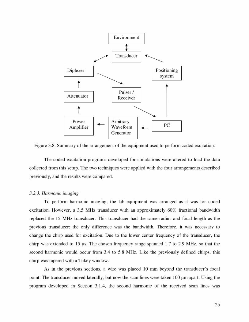
a series of instruments before exciting the transducer. Figure 3.8 is a diagram of the equipment.

A power amplifier (ENI, Rochester, NY), diplexer (Ritec, Warwick, RI), and the arbitrary

waveform generator were used, in addition to the equipment used for standard pulse excitation.

The same transducer receives the echo response, which is read by the pulser-receiver and

transmitted to the computer.

25

Figure 3.8. Summary of the arrangement of the equipment used to perform coded excitation.

The coded excitation programs developed for simulations were altered to load the data

collected from this setup. The two techniques were applied with the four arrangements described

previously, and the results were compared.

3.2.3. Harmonic imaging

To perform harmonic imaging, the lab equipment was arranged as it was for coded

excitation. However, a 3.5 MHz transducer with an approximately 60% fractional bandwidth

replaced the 15 MHz transducer. This transducer had the same radius and focal length as the

previous transducer; the only difference was the bandwidth. Therefore, it was necessary to

change the chirp used for excitation. Due to the lower center frequency of the transducer, the

chirp was extended to 15 µs. The chosen frequency range spanned 1.7 to 2.9 MHz, so that the

second harmonic would occur from 3.4 to 5.8 MHz. Like the previously defined chirps, this

chirp was tapered with a Tukey window.

As in the previous sections, a wire was placed 10 mm beyond the transducer’s focal

point. The transducer moved laterally, but now the scan lines were taken 100 µm apart. Using the

program developed in Section 3.1.4, the second harmonic of the received scan lines was

Transducer

PC

Pulser /

Receiver

Positioning

system

Environment

Arbitrary

Waveform

Generator

Power

Amplifier

Attenuator

Diplexer

26

extracted with pulse inversion. A Wiener filter was used to compress the chirp, and SAFT

restored lateral resolution.

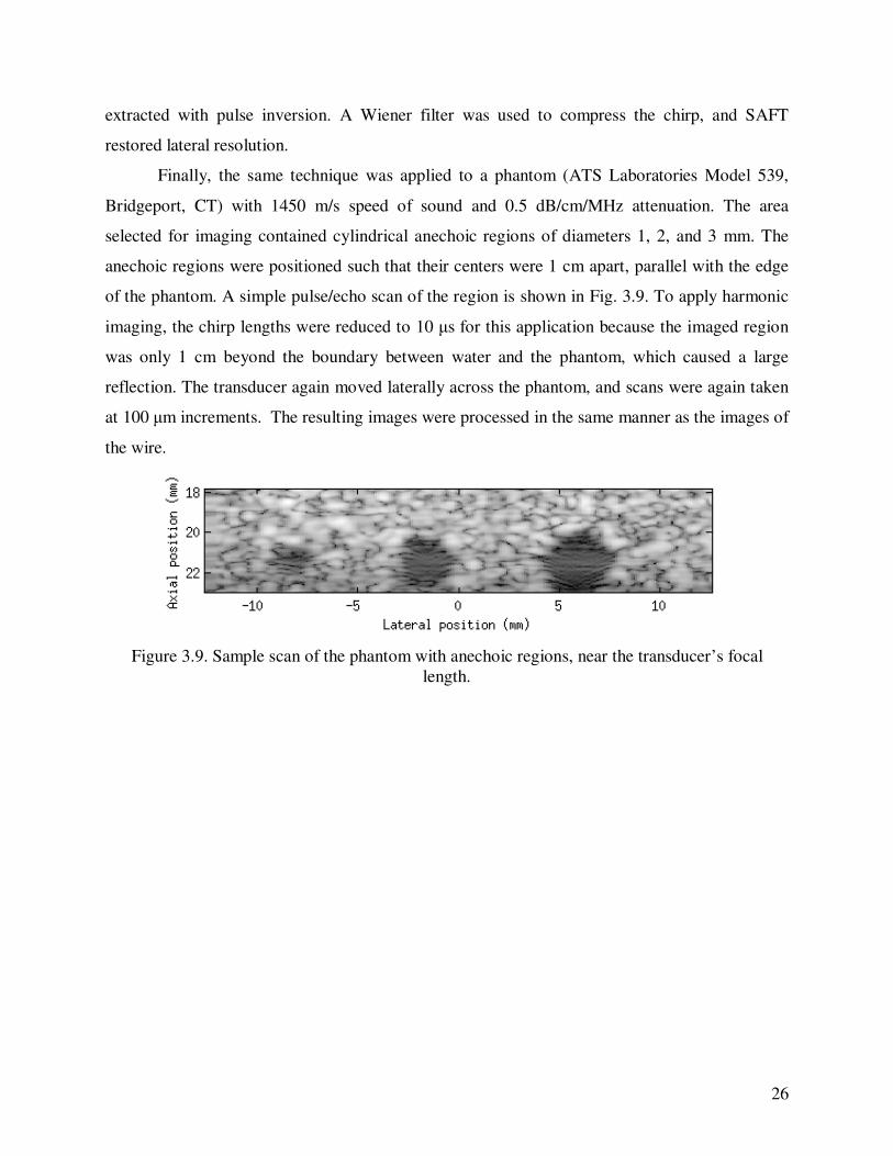
Finally, the same technique was applied to a phantom (ATS Laboratories Model 539,

Bridgeport, CT) with 1450 m/s speed of sound and 0.5 dB/cm/MHz attenuation. The area

selected for imaging contained cylindrical anechoic regions of diameters 1, 2, and 3 mm. The

anechoic regions were positioned such that their centers were 1 cm apart, parallel with the edge

of the phantom. A simple pulse/echo scan of the region is shown in Fig. 3.9. To apply harmonic

imaging, the chirp lengths were reduced to 10 µs for this application because the imaged region

was only 1 cm beyond the boundary between water and the phantom, which caused a large

reflection. The transducer again moved laterally across the phantom, and scans were again taken

at 100 µm increments. The resulting images were processed in the same manner as the images of

the wire.

Figure 3.9. Sample scan of the phantom with anechoic regions, near the transducer’s focal

length.

27

CHAPTER 4: RESULTS

4.1. Synthetic Aperture with a Virtual Source

4.1.1. Synthetic aperture simulations

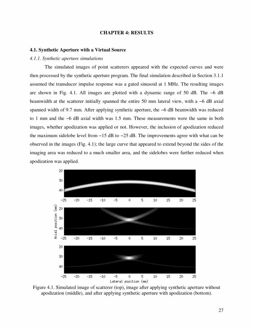
The simulated images of point scatterers appeared with the expected curves and were

then processed by the synthetic aperture program. The final simulation described in Section 3.1.1

assumed the transducer impulse response was a gated sinusoid at 1 MHz. The resulting images

are shown in Fig. 4.1. All images are plotted with a dynamic range of 50 dB. The −6 dB

beamwidth at the scatterer initially spanned the entire 50 mm lateral view, with a −6 dB axial

spanned width of 9.7 mm. After applying synthetic aperture, the −6 dB beamwidth was reduced

to 1 mm and the −6 dB axial width was 1.5 mm. These measurements were the same in both

images, whether apodization was applied or not. However, the inclusion of apodization reduced

the maximum sidelobe level from −15 dB to −25 dB. The improvements agree with what can be

observed in the images (Fig. 4.1); the large curve that appeared to extend beyond the sides of the

imaging area was reduced to a much smaller area, and the sidelobes were further reduced when

apodization was applied.

Figure 4.1. Simulated image of scatterer (top), image after applying synthetic aperture without

apodization (middle), and after applying synthetic aperture with apodization (bottom).

28

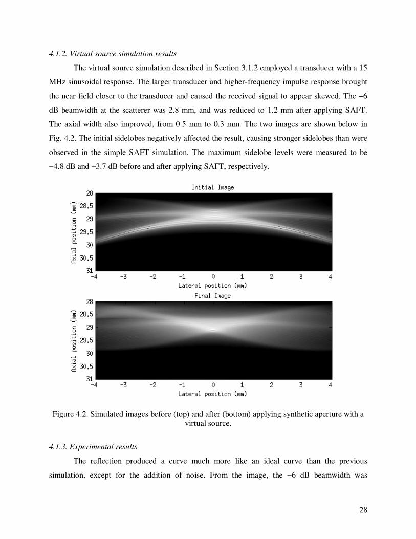
4.1.2. Virtual source simulation results

The virtual source simulation described in Section 3.1.2 employed a transducer with a 15

MHz sinusoidal response. The larger transducer and higher-frequency impulse response brought

the near field closer to the transducer and caused the received signal to appear skewed. The −6

dB beamwidth at the scatterer was 2.8 mm, and was reduced to 1.2 mm after applying SAFT.

The axial width also improved, from 0.5 mm to 0.3 mm. The two images are shown below in

Fig. 4.2. The initial sidelobes negatively affected the result, causing stronger sidelobes than were

observed in the simple SAFT simulation. The maximum sidelobe levels were measured to be

−4.8 dB and −3.7 dB before and after applying SAFT, respectively.

Figure 4.2. Simulated images before (top) and after (bottom) applying synthetic aperture with a

virtual source.

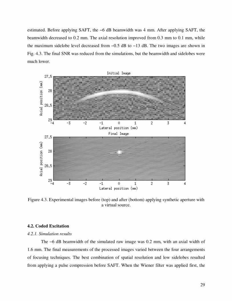
4.1.3. Experimental results

The reflection produced a curve much more like an ideal curve than the previous

simulation, except for the addition of noise. From the image, the −6 dB beamwidth was

29

estimated. Before applying SAFT, the −6 dB beamwidth was 4 mm. After applying SAFT, the

beamwidth decreased to 0.2 mm. The axial resolution improved from 0.3 mm to 0.1 mm, while

the maximum sidelobe level decreased from −0.5 dB to −13 dB. The two images are shown in

Fig. 4.3. The final SNR was reduced from the simulations, but the beamwidth and sidelobes were

much lower.

Figure 4.3. Experimental images before (top) and after (bottom) applying synthetic aperture with

a virtual source.

4.2. Coded Excitation

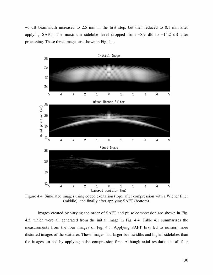
4.2.1. Simulation results

The −6 dB beamwidth of the simulated raw image was 0.2 mm, with an axial width of

1.6 mm. The final measurements of the processed images varied between the four arrangements

of focusing techniques. The best combination of spatial resolution and low sidelobes resulted

from applying a pulse compression before SAFT. When the Wiener filter was applied first, the

30

−6 dB beamwidth increased to 2.5 mm in the first step, but then reduced to 0.1 mm after

applying SAFT. The maximum sidelobe level dropped from −8.9 dB to −14.2 dB after

processing. These three images are shown in Fig. 4.4.

Figure 4.4. Simulated images using coded excitation (top), after compression with a Wiener filter

(middle), and finally after applying SAFT (bottom).

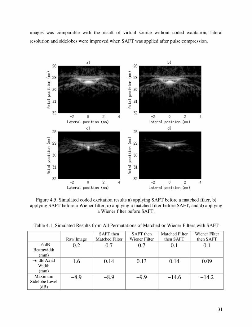
Images created by varying the order of SAFT and pulse compression are shown in Fig.

4.5, which were all generated from the initial image in Fig. 4.4. Table 4.1 summarizes the

measurements from the four images of Fig. 4.5. Applying SAFT first led to noisier, more

distorted images of the scatterer. These images had larger beamwidths and higher sidelobes than

the images formed by applying pulse compression first. Although axial resolution in all four

31

images was comparable with the result of virtual source without coded excitation, lateral

resolution and sidelobes were improved when SAFT was applied after pulse compression.

Figure 4.5. Simulated coded excitation results a) applying SAFT before a matched filter, b)

applying SAFT before a Wiener filter, c) applying a matched filter before SAFT, and d) applying

a Wiener filter before SAFT.

Table 4.1. Simulated Results from All Permutations of Matched or Wiener Filters with SAFT

Raw Image

SAFT then Matched Filter

SAFT then Wiener Filter

Matched Filter then SAFT

Wiener Filter then SAFT

−6 dB

Beamwidth

(mm)

0.2 0.7 0.7 0.1 0.1

−6 dB Axial

Width

(mm)

1.6 0.14 0.13 0.14 0.09

Maximum Sidelobe Level

(dB)

−8.9 −8.9 −9.9 −14.6 −14.2

32

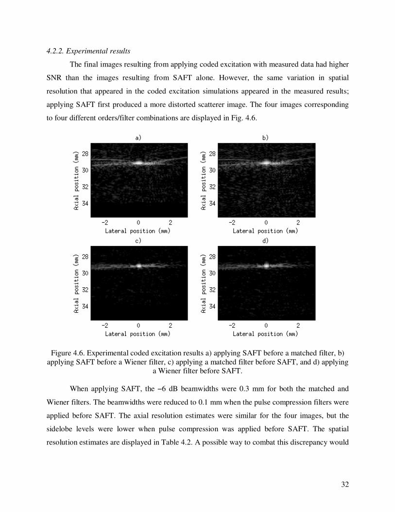
4.2.2. Experimental results

The final images resulting from applying coded excitation with measured data had higher

SNR than the images resulting from SAFT alone. However, the same variation in spatial

resolution that appeared in the coded excitation simulations appeared in the measured results;

applying SAFT first produced a more distorted scatterer image. The four images corresponding

to four different orders/filter combinations are displayed in Fig. 4.6.

Figure 4.6. Experimental coded excitation results a) applying SAFT before a matched filter, b)

applying SAFT before a Wiener filter, c) applying a matched filter before SAFT, and d) applying

a Wiener filter before SAFT.

When applying SAFT, the −6 dB beamwidths were 0.3 mm for both the matched and

Wiener filters. The beamwidths were reduced to 0.1 mm when the pulse compression filters were

applied before SAFT. The axial resolution estimates were similar for the four images, but the

sidelobe levels were lower when pulse compression was applied before SAFT. The spatial

resolution estimates are displayed in Table 4.2. A possible way to combat this discrepancy would

33

be to reverse the chirp, so that the distortion would occur primarily at the lower frequencies and

be less distorting.

Table 4.2. Measured Results from All Permutations of Matched or Wiener Filters with SAFT

Raw Image

SAFT then

Matched Filter

SAFT then

Wiener Filter

Matched Filter

then SAFT

Wiener Filter

then SAFT

−6 dB

Beamwidth

(mm)

1.1 0.3 0.3 0.1 0.1

−6 dB Axial Width

(mm)

1.7 0.11 0.14 0.15 0.14

Maximum

Sidelobe Level (dB)

0 −11.7 −12.2 −19.8 −20.1

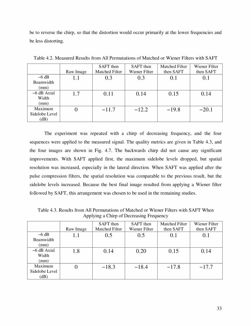
The experiment was repeated with a chirp of decreasing frequency, and the four

sequences were applied to the measured signal. The quality metrics are given in Table 4.3, and

the four images are shown in Fig. 4.7. The backwards chirp did not cause any significant

improvements. With SAFT applied first, the maximum sidelobe levels dropped, but spatial

resolution was increased, especially in the lateral direction. When SAFT was applied after the

pulse compression filters, the spatial resolution was comparable to the previous result, but the

sidelobe levels increased. Because the best final image resulted from applying a Wiener filter

followed by SAFT, this arrangement was chosen to be used in the remaining studies.

Table 4.3. Results from All Permutations of Matched or Wiener Filters with SAFT When

Applying a Chirp of Decreasing Frequency

Raw Image

SAFT then Matched Filter

SAFT then Wiener Filter

Matched Filter then SAFT

Wiener Filter then SAFT

−6 dB

Beamwidth (mm)

1.1 0.5 0.5 0.1 0.1

−6 dB Axial

Width

(mm)

1.8 0.14 0.20 0.15 0.14

Maximum

Sidelobe Level

(dB)

0 −18.3 −18.4 −17.8 −17.7

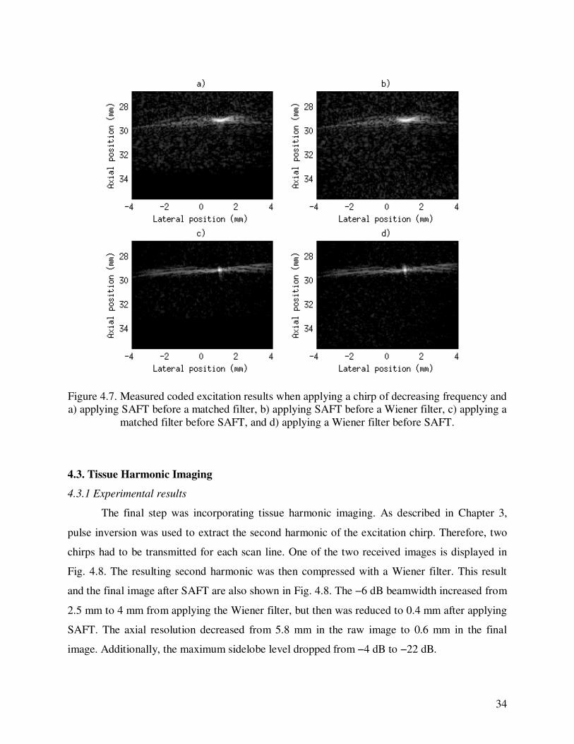
34

Figure 4.7. Measured coded excitation results when applying a chirp of decreasing frequency and

a) applying SAFT before a matched filter, b) applying SAFT before a Wiener filter, c) applying a

matched filter before SAFT, and d) applying a Wiener filter before SAFT.

4.3. Tissue Harmonic Imaging

4.3.1 Experimental results

The final step was incorporating tissue harmonic imaging. As described in Chapter 3,

pulse inversion was used to extract the second harmonic of the excitation chirp. Therefore, two

chirps had to be transmitted for each scan line. One of the two received images is displayed in

Fig. 4.8. The resulting second harmonic was then compressed with a Wiener filter. This result

and the final image after SAFT are also shown in Fig. 4.8. The −6 dB beamwidth increased from

2.5 mm to 4 mm from applying the Wiener filter, but then was reduced to 0.4 mm after applying

SAFT. The axial resolution decreased from 5.8 mm in the raw image to 0.6 mm in the final

image. Additionally, the maximum sidelobe level dropped from −4 dB to −22 dB.

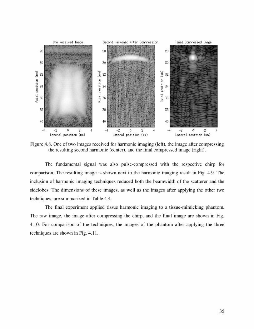
35

Figure 4.8. One of two images received for harmonic imaging (left), the image after compressing

the resulting second harmonic (center), and the final compressed image (right).

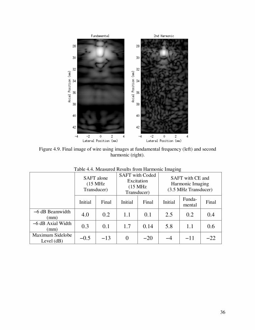
The fundamental signal was also pulse-compressed with the respective chirp for

comparison. The resulting image is shown next to the harmonic imaging result in Fig. 4.9. The

inclusion of harmonic imaging techniques reduced both the beamwidth of the scatterer and the

sidelobes. The dimensions of these images, as well as the images after applying the other two

techniques, are summarized in Table 4.4.

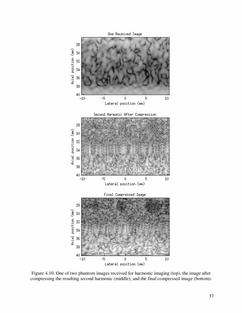
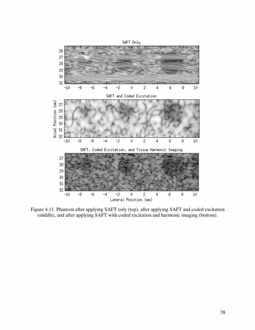
The final experiment applied tissue harmonic imaging to a tissue-mimicking phantom.

The raw image, the image after compressing the chirp, and the final image are shown in Fig.

4.10. For comparison of the techniques, the images of the phantom after applying the three

techniques are shown in Fig. 4.11.

36

Figure 4.9. Final image of wire using images at fundamental frequency (left) and second

harmonic (right).

Table 4.4. Measured Results from Harmonic Imaging

SAFT alone

(15 MHz

Transducer)

SAFT with Coded

Excitation

(15 MHz

Transducer)

SAFT with CE and

Harmonic Imaging

(3.5 MHz Transducer)

Initial Final Initial Final Initial Funda-

mental Final

−6 dB Beamwidth

(mm) 4.0 0.2 1.1 0.1 2.5 0.2 0.4

−6 dB Axial Width

(mm) 0.3 0.1 1.7 0.14 5.8 1.1 0.6

Maximum Sidelobe

Level (dB) −0.5 −13 0 −20 −4 −11 −22

37

Figure 4.10. One of two phantom images received for harmonic imaging (top), the image after

compressing the resulting second harmonic (middle), and the final compressed image (bottom).

38

Figure 4.11. Phantom after applying SAFT only (top), after applying SAFT and coded excitation

(middle), and after applying SAFT with coded excitation and harmonic imaging (bottom).

39

CHAPTER 5: CONCLUSION

5.1. Discussion of Results

5.1.1. Synthetic aperture with a virtual source

Although the simulations provided realistic data, the noise, attenuation, and speckle that

exist in real systems were not simulated. These effects appeared to be tolerated by SAFT.

Although the SNR was lower than simulated, the clarity and sidelobes of the final image from

measured data appeared better than the simulated result.

5.1.2. Coded excitation

The measured data led to a final result of higher SNR than was observed before

integrating coded excitation. The coding helped to increase the SNR. However, the sidelobes

became much more visible. Additionally, some of the arrangements of the techniques caused

more distortion than the others.

The results in Chapter 4 indicated that spatial resolution was better when applying pulse

compression before applying SAFT than when applying SAFT first. This effect suggests that

synthetic aperture is not a linear process and can cause distortion. In this situation, a major

contributor to the distortion was the length of the chirp.

SAFT focuses at each point by calculating a curve corresponding to the point, and the

shape of that curve changes with axial distance. While the chirp length did not change with angle

or distance, the calculated curves used by SAFT did change. As a result, the curve at the

beginning of a chirp did not match the curve at the end of the chirp, causing distortion that was

increased by a longer signal. The distorted chirp did not match with the Wiener filter, reducing

its effectiveness. This problem was eliminated when the Wiener filter compressed the chirp

before SAFT was applied.

5.1.3. Harmonic imaging

Although the measured −6 dB beamwidth using tissue harmonic imaging was larger than

the measured beamwidth without harmonic imaging, it must be noted that the transducer’s

resonant frequency was only 23% of the previous transducer’s resonant frequency. A lower

frequency corresponds to a longer wavelength, which diminishes spatial resolution. Therefore, an

40

increase from 0.1 mm to 0.4 mm when switching from a 15 MHz transducer to a 3.5 MHz

transducer actually is a slight improvement. The sidelobes were also less prominent when using

SAFT and coded excitation at the fundamental frequency. However, the speckle increased and

the SNR decreased, likely due to the decreased signal strength of the transducer at the

frequencies above and below the resonant frequency.

5.2. Conclusions

This study verified previous work that synthetic aperture with a virtual source element can allow

imaging beyond a transducer’s focal length. Additionally, frequency-coded excitation using a

linear chirp can be incorporated into this setup. However, SAFT causes distortion in longer

signals. Therefore, in processing the received image, it is most practical to apply a Wiener filter

or another form of time compression first and then apply synthetic aperture focusing to the

compressed scan lines.

Tissue harmonic imaging can also be applied using these techniques. This process

successfully improved lateral resolution, reduced sidelobes, and increased SNR. However,

speckle was more pronounced than when coded excitation and SAFT were used without

harmonic imaging.

5.3. Suggestions for Future Work

This study has shown that synthetic aperture with a virtual source, coded excitation, and tissue

harmonic imaging can be combined to image beyond the focal length of a transducer. However,

not all aspects of the combined technique have been studied. One area that was not explored was

the maximum depth at which the technique is practical.

A focusing technique is not useful unless it has an application. In order to be medically

useful, a technique would need to work in real tissue. This study did not test the effectiveness of

SAFT, coded excitation, or tissue harmonic imaging when they are applied to real tissue data.

Only preliminary data were gathered using these techniques on a tissue-mimicking phantom.

More study in this vein would be necessary to verify the effectiveness of the process.

41

REFERENCES

[1] C. H. Frazier and W. D. O’Brien, “Synthetic aperture techniques with a virtual source

element,” IEEE Transactions on Ultrasonics, Ferroelectrics, and Frequency Control,

vol. 45, no. 1, pp. 196-207, Jan. 1998.

[2] M.-H. Bae and M.-K. Jeong, “A study of synthetic-aperture imaging with virtual source

elements in B-mMode ultrasound imaging systems,” IEEE Transactions on Ultrasonics,

Ferroelectrics, and Frequency Control, vol. 47, no. 6, pp. 1510-1519, Nov. 2000.

[3] R. Y. Chiao and X. Hao, “Coded excitation for diagnostic ultrasound: System developer’s

perspective,” IEEE Transactions on Ultrasonics, Ferroelectrics, and Frequency Control,

vol. 52, no. 2, pp. 160-170, Feb. 2005.

[4] T. Misaridis and J. A. Jensen, “Use of modulated excitation signals in medical

ultrasound. Part I: Basic concepts and expected benefits,” IEEE Transactions on

Ultrasonics, Ferroelectrics, and Frequency Control, vol. 52, no. 2, pp. 177-1891, Feb.

2005.

[5] M. A. Averkiou, “Tissue harmonic imaging,” in 2000 IEEE Ultrasonics Symposium, pp.

1563-1572.

[6] J. A. Jensen, “Field: A program for simulating ultrasound systems,” Medical &

Biological Engineering & Computing, vol. 34, supplement 1, part 1, pp. 351-353, 1996.

[7] J. A. Jensen and N. B. Svendsen, “Calculation of pressure fields from arbitrarily shaped,

apodized, and excited ultrasound transducers,” IEEE Transactions on Ultrasonics,

Ferroelectrics, and Frequency Control, vol. 39, pp. 262-267, 1992.