Applying species distribution modelling to a data poor, pelagic fishcomplex: the ocean sunfishes

Phillips, N. D., Reid, N., Thys, T., Harrod, C., Payne, N. L., Morgan, C. A., White, H. J., Porter, S., & Houghton,J. D. R. (2017). Applying species distribution modelling to a data poor, pelagic fish complex: the oceansunfishes. Journal of Biogeography. https://doi.org/10.1111/jbi.13033

Published in:Journal of Biogeography

Document Version:Peer reviewed version

Queen's University Belfast - Research Portal:Link to publication record in Queen's University Belfast Research Portal

Publisher rights© 2017 John Wiley & Sons Ltd. This work is made available online in accordance with the publisher’s policies. Please refer to any applicableterms of use of the publisher.

General rightsCopyright for the publications made accessible via the Queen's University Belfast Research Portal is retained by the author(s) and / or othercopyright owners and it is a condition of accessing these publications that users recognise and abide by the legal requirements associatedwith these rights.

Take down policyThe Research Portal is Queen's institutional repository that provides access to Queen's research output. Every effort has been made toensure that content in the Research Portal does not infringe any person's rights, or applicable UK laws. If you discover content in theResearch Portal that you believe breaches copyright or violates any law, please contact openaccess@qub.ac.uk.

Download date:30. Nov. 2021

1  

Original Article 1 

Applying Species Distribution Modelling to a Data Poor, Pelagic Fish Complex: 2 

The Ocean Sunfishes 3 

4 

N.D. Phillips*1, N. Reid1,2, T. Thys3, C. Harrod4, N. Payne5, C. Morgan6, H.J. White1, 5 

S. Porter1, J.D.R. Houghton1,2 6 

7 

1School of Biological Sciences, Queen’s University Belfast MBC Building, 97 Lisburn Road, Belfast, BT9 7BL, 8 

U.K., 2Institute of Global Food Security, Queen’s University Belfast, 18-30 Malone Road, Belfast, BT9 5BN, 9 

U.K., 3California Academy of Science, 55 Music Concourse Drive, Golden Gate Park, San Francisco, CA, 10 

94118 U.S.A., 4Instituto de Ciencias Naturales Alexander von Humboldt, Universidad de Antofagasta, Avenida 11 

Angamos 601, Antofagasta, Chile, 5University of Roehampton, Holybourne Avenue, London, SW15 4JD, 12 

Cooperative Institute for Marine Resources Studies, Oregon State University, 2030 S. Marine Science Center, 13 

Newport, OR 97365 14 

15 

*Author to whom correspondence should be addressed: Natasha Phillips, Queen’s University 16 

Belfast, Medical Biology Centre, 97 Lisburn Road, Belfast, BT9 7AE, 17 

nphillips01@qub.ac.uk 18 

19 

Running head: Distribution and seasonal movements of ocean sunfishes 20 

21 

Keywords: Biogeography, Environmental Niche Models, Marine, Migration, Mola, 22 

sunfishes, Spatial Ecology 23 

2  

Abstract 24 

25 

Aim 26 

Conservation management of vulnerable species requires detailed knowledge of their spatial 27 

and temporal distribution patterns. Within this context species distribution modelling (SDM) 28 

can provide insights into the spatial ecology of rarely encountered species and is used here to 29 

explore the distribution pattern of ocean sunfishes (Mola mola and M. ramsayi). Both species 30 

are prone to high levels of bycatch and are classified respectively as Globally Vulnerable and 31 

Not Assessed by the IUCN; although their overall range and drivers of distribution remain 32 

poorly defined. Here, we constructed suitable habitat models for Mola spp. on a global scale 33 

and considered how these change seasonally to provide a much needed baseline for future 34 

management. 35 

36 

Location 37 

Global. 38 

39 

Methods 40 

Sighting records collected between 2000 and 2015 were used to build SDMs and provided the 41 

first global overview of sunfish seasonal distribution. Post-hoc analyses provided a 42 

quantitative assessment of seasonal changes in total range extent and latitudinal shifts in 43 

suitable habitat. 44 

45 

Results 46 

Mola is a widely distributed genus; however, sightings exhibited significant spatial clustering 47 

most notably in coastal regions. SDMs suggested that Mola presence was strongly dependant 48 

on sea surface temperatures with highest probability of presence between 16 and 23°C. The 49 

models identified significant variation in seasonal range extent with latitudinal shifts 50 

throughout the year; although large areas of suitable year-round habitat exist globally. 51 

52 

Main conclusions 53 

We provided the first assessment of Mola distribution on a global scale, with evidence of a 54 

wide latitudinal range and significant clustering in localised ‘hotspots’ (notably between 40-55 

50°N). By assessing the results of SDMs alongside evidence from published satellite tagging 56 

studies, we suggest that the species within the genus Mola are highly mobile, acting as 57 

3  

facultative seasonal migrants. By identifying key suitable habitat alongside potential 58 

movement paths, this study provides a baseline that can be used in active conservation 59 

management of the genus. 60 

4  

Introduction 61 

Conservation management efforts are dependent on a detailed understanding of the spatial 62 

distribution, biogeography and ecology of target species (Ferrier et al., 2002; Ricklefs, 2004; 63 

Rushton et al., 2004). For widespread or cryptic species this can pose significant challenges 64 

(Pearson et al., 2007; Rissler & Apodaca, 2007). Species distribution models (SDMs, also 65 

known as ecological niche models, species-habitat models or predictive habitat models) 66 

assess the complex relationship between species occurrence records and environmental 67 

variation, even from limited datasets, and offers insight into habitat suitability both spatially 68 

and temporally (Elith & Leathwick, 2009; Franklin, 2009). For little known oceanic species, 69 

such methods can provide a key starting point in understanding complex, wide-ranging 70 

distribution patterns and the mechanisms driving environmental tolerances (Elith et al., 71 

2006). 72 

One such family of oceanic taxa, the ocean sunfishes (or Molidae), are often described as 73 

rare, inactive drifters (Pope et al., 2010), however recent studies have revealed high density 74 

aggregations in coastal waters (e.g. Silvani et al., 1999; Pope et al., 2010; Syväranta et al., 75 

2012), sustained long distance swimming of ~48 km per day (e.g. Cartamil & Lowe, 2004; 76 

Nakamura et al., 2015; Thys et al., 2015) and repeated deep-diving to mesopelagic depths 77 

foraging for gelatinous prey (e.g. Cartamil & Lowe, 2004; Nakamura et al., 2015). Such 78 

observations suggest that this is an active, highly motile taxon (Cartamil & Lowe, 2004), with 79 

a broad trophic niche (e.g. Harrod et al., 2013; Nakamura & Sato, 2014; Sousa et al., 2016a) 80 

and capable of travelling significant distances in a directed manner (see review, Pope et al., 81 

2010). This suggests that Mola may have more complex ecology than previously thought 82 

(Syväranta et al., 2012), which poses broader implications for sustainable management. Such 83 

insight is important in light of current bycatch levels (Silvani et al., 1999; Cartamil & Lowe, 84 

2004; Pope et al., 2010), such as the reported capture of > 36 000 individuals per annum in 85 

5  

Mediterranean drift gillnets (Petersen & McDonell, 2007). Bycatch numbers coupled with 86 

impacts of large-scale target fisheries, led to a recent IUCN Red List classification of Mola 87 

mola (L. 1758) as globally Vulnerable (Jing et al., 2010) and Data Deficient in Europe (see 88 

Table 1, Appendices). This Red Listing represents a tentative first step towards future 89 

management strategies and highlights areas of sunfish ecology that require further research, 90 

such as knowledge of their distribution and movements, which currently restricts 91 

management and conservation efforts. 92 

Anecdotal evidence collated in a review by Pope et al. (2010) suggested that the Molidae 93 

(see Table 1. Appendices) have a pan-global distribution within temperate and tropical 94 

latitudes, although limited sighting records and inherent difficulties in species identification 95 

have led to problems in delineating species-specific ranges and seasonal movement patterns. 96 

Recent high-profile reports of ocean sunfishes at high latitudes, such as in Alaska (Dobbyn, 97 

2015), have led many media outlets to speculate as to why these species are “suddenly” 98 

appearing so far north. However, without baseline data on the range extent of ocean 99 

sunfishes, it is difficult to know whether they have undergone recent expansion and, if so, 100 

what might be driving such changes. Although taken to be widespread (Cartamil & Lowe, 101 

2004), it is not yet known if ocean sunfishes adhere consistently to a migratory paradigm 102 

(whether obligate or facultative). Evidence from multiple studies, using satellite tags and 103 

accelerometer derived dead-reckoning (e.g. Sims et al., 2009; Dewar et al., 2010; Nakamura 104 

et al., 2015; Thys et al., 2015), suggests that Mola in temperate and subtropical regions may 105 

move to equatorial latitudes during autumn, for example, into UK and Japanese waters. 106 

However, other studies using satellite tracking (Hays et al., 2009) and dietary analysis 107 

(Harrod et al., 2013) suggest year-round, or at least long-term, residence in some regions, 108 

including in Mediterranean and South African waters. The results from these studies support 109 

6  

suggestions of distinct, local populations with differing drivers of distribution; however, there 110 

is a paucity of evidence across wide spatio-temporal scales. 111 

From a broader conservation perspective, the IUCN states that creating a “comprehensive, 112 

objective global approach for evaluating the conservation status of [all] species [is important 113 

in order to] inform and catalyse action for biodiversity conservation” (IUCN, 2016). In line 114 

with this statement, this study uses SDM to provide an initial assessment of the global 115 

distribution pattern of a vulnerable marine genus that is plagued with species-specific 116 

identification problems. We present basic life history information for the genus Mola and its 117 

seasonal range extent in relation to key predictive environmental parameters. This study 118 

provides an objective evidence base critical to providing a full IUCN Red Listing, upon 119 

which international management decisions can be founded. 120 

121 

Materials and Methods 122 

Data sources and manipulation 123 

Global sightings of Mola were collected from public databases, published papers and 124 

fisheries logs (see Appendix S1). A total of 14 953 sightings, recorded between the years 125 

1758 and 2015, were compiled before specific criteria were set for standardising the dataset. 126 

This study aimed to assess the distribution of the genus Mola which currently contains two 127 

species. Mola is easily distinguishable from other genera in the Molidae (Ranzania and 128 

Masturus, see Table 1. Appendices), due to its differing morphology, and therefore potential 129 

for confusion is limited. We accept that misidentification is possible, but by maintaining a 130 

conservative approach to data acquisition (i.e. by removing records not identified to genus), 131 

we have tried to mitigate this risk. Any incomplete records (missing location or date of 132 

observation) were removed. All sighting locations were converted to decimal degrees, and 133 

mapped using ARCGIS 10.3.1 (ESRI, California, USA) and all locations that erroneously fell 134 

7  

on land were removed. Although the sightings dataset extended over 257 years, 79% of 135 

sightings occurred between 2000 and 2015. Therefore only this subset of 5 419 sightings was 136 

retained for further analysis. These sightings were divided into each quarter of the year (Jan-137 

Mar, Apr-May, Jun-Aug and Sep-Dec) and matched with recent climate data available 138 

through online data sharing platforms. 139 

140 

Environmental parameters 141 

Climate data with near global oceanic coverage described surface oceanography at a 142 

resolution of one decimal degree delineated as a cellular matrix. The most recently collected 143 

dynamic parameters were selected and of these, sea surface temperature, nitrate, oxygen and 144 

chlorophyll concentration were averaged over three month periods suited to generating 145 

seasonal summaries (Jan-Mar, Apr-May, Jun-Aug and Sep-Dec). The datasets included sea 146 

surface temperature averaged from 2005 to 2012 (NOAA, 2015), nitrate and oxygen 147 

concentrations averaged from 1955 to 2012 (NOAA, 2015) and chlorophyll concentration 148 

averaged from 2002 to 2012 (NASA, 2012). Despite the extensive coverage provided by 149 

satellite data, the limitations of this dataset must be acknowledged; such as the lower quality 150 

data from nearshore or frequently clouded environments (Smith et al., 2013). Of all the 151 

parameters included, bathymetry was the only static variable recorded from a 2002-2003 152 

global survey (NASA, 2003). If climatic data were missing from the decimal degree cell in 153 

which a sighting was recorded, it was removed from the analysis (leaving n = 4 985 154 

sightings). 155 

156 

Data validation 157 

Since all Mola data collected were ‘presence only’ sightings, we implemented a bias file as a 158 

proxy of survey effort to indicate the likelihood of being encountered and recorded, as 159 

8  

presence-absence models perform better than presence only models (Elith et al., 2006). Since 160 

true absence data were not available, we followed established methods to construct a ‘bias 161 

file’ (e.g. Phillips et al., 2009; Aguirre-Gutierrez et al., 2013: Pokharel et al., 2016). This 162 

process requires the identification of a suitable proxy species (termed a target group) for 163 

which further presence data were available (e.g. Ponder et al., 2001: Anderson, 2003). We 164 

chose to use the leatherback turtle, Dermochelys coriacea (Vandelli, 1761) as it is suggested 165 

to inhabit similar environments to ocean sunfishes (Hays et al., 2009). Moreover, the species 166 

is an active predator of gelatinous zooplankton and conforms to the seasonal migration 167 

paradigm suggested for sunfishes (see Pope review, 2009), while being subject to similar sea 168 

surface and coastal observation biases (Houghton et al., 2006; Hays et al., 2009). Leatherback 169 

turtle sightings data were downloaded from the Global Biodiversity Information Facility 170 

sightings database (GBIF, 2015). The use of target group data has been reported to provide a 171 

considerable improvement in model performance, providing more realistic data than taking 172 

pseudo-absences from sites that have not been sampled at all (e.g. Phillips, 2009; Mateo et 173 

al., 2010; Aguirre-Gutierrez et al., 2013). The rationale here is that leatherback sightings 174 

provided a proxy for recorder presence with the inference that ocean sunfish sightings would 175 

have been recorded concurrently if present. Correspondingly, these locations were used to 176 

generate ocean sunfish pseudo-absence data (n = 434) to train SDMs. 177 

178 

Statistical Analysis & SDMs 179 

The distribution of Mola was mapped globally and a minimum convex hull containing all 180 

sightings created to satisfy the IUCN Red List range map requirements. Owing to the cryptic 181 

speciation within Mola, such range mapping was constrained to genus level. 182 

A cluster analysis of sightings was performed using a Clark-Evans nearest neighbour test 183 

(Clark & Evans, 1954) using the R x64 3.2.2 (R Development Core Team, 2008) package 184 

9  

‘spatstat’ (Baddeley et al., 2015). The degree of grouping was determined using a correction 185 

cumulative distribution function and a Monte Carlo test to provide a probability value. 186 

Climatic data were tested for collinearity using Pearson’s correlation, before SDMs were 187 

produced using the R package ‘Biomod2’ (Thuiller et al., 2015). Seven SDM types were 188 

assessed including: surface range envelopes (SRE, quant = 0.025), classification tree analysis 189 

(CTA, CV.tree = 50), random forest (RF), multiple adaptive regression splines (MARS), 190 

flexible discriminant analysis (FDA), generalised linear models (GLM, type = simple) and 191 

generalised additive models (GAM, spline = 3). The models were designed with an 80:20 192 

data split for training and testing and run with a 5 000 fold cross validation. All models used 193 

in Biomod2 were run using the default settings recommended by Thuiller et al. (2010). Using 194 

this model design, the seasonal distribution of Mola was predicted using matched sightings 195 

and environmental data from each quarter of the year. 196 

Model evaluation statistics were calculated including the Kappa value (k), true skill 197 

statistic (TSS) and area under the curve (AUC) of the receiver operating characteristic 198 

(ROC). These evaluation metrics are frequently used to evaluate SDM performance, although 199 

AUC values have recently been criticised for overestimating performance by including large 200 

areas of absence data (Lobo et al. 2008; Leach et al. 2015). Popular alternatives also have 201 

limitations, such as TSS which is calculated from sensitivity and specificity, which 202 

themselves can contain misleading commission errors (Leach et al. 2015). The Kappa value 203 

provides a more objective measure of prediction accuracy, although this can also produce 204 

commission errors (Leach et al. 2015), but it provides accepted thresholds used in model 205 

evaluation. Here, we present each evaluation metric for all models however, the final 206 

evaluation of model accuracy used Kappa. 207 

The optimal SDM was selected from those with a Kappa > 0.4 (see Table 2), as this 208 

threshold has been widely used in a range of published work (Landis et al., 1977; Altman, 209 

10  

1990; Allouche et al., 2006; Leach et al. 2015). The random forest model was the single best 210 

approximating model selected for further analysis and re-run with 100% of the sightings data 211 

to predict the seasonal probability of Mola presence globally. 212 

To assess the seasonal range extent of Mola, the proportion of cells predicted with a 213 

probability of presence > 0.7 was calculated and tested with a 4-sample test for equality of 214 

proportions without continuity correction. As the distribution data were strongly skewed, 215 

non-parametric tests were used. Due to uneven sampling, data were divided into Northern 216 

and Southern Hemispheres and the predicted range extent of Mola examined by plotting box 217 

and whisker diagrams of the latitudinal range divided by season and compared statistically 218 

using a Kruskal-Wallis test. To assess if individual Mola move seasonally in accordance with 219 

the model predictions, the latitude of all sightings were plotted against the Julian day of the 220 

year on which they were recorded and fitted with a locally weighted scatterplot smoothing 221 

curve (LOESS). 222 

223 

Results 224 

Mola observations were distributed globally (Fig. 1a and b) but with significant clustering (z 225 

= 0.335, p < 0.05), with aggregations in North American and European coastal waters 226 

predominately between 20-60°N, and peaking at 50°N (Fig. 2). 227 

Nitrate and oxygen concentrations were significantly correlated (r = 0.88, p < 0.001), and 228 

since nitrate is used here as a proxy for productivity, it was removed to avoid leverage in 229 

statistical models. The random forest model had the highest model evaluation statistic values 230 

(mean values of 5 model runs: Kappa = 0.63, TSS: 0.72, ROC: 0.93) and were thus chosen as 231 

the optimal SDM technique. 232 

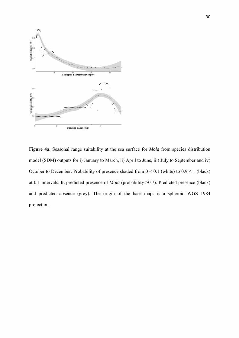
Random forest LOESS curves suggested Mola presence was associated with shallow, 233 

temperate (7-23°C), relatively low productivity (chlorophyll < 125mg/m3), oxygen rich (> 234 

11  

4ml/L) coastal waters (Fig. 3a-d). However, cells predicted to have a probability of presence 235 

> 0.7 were widespread in all seasons resulting in a pan-global distribution in surface waters 236 

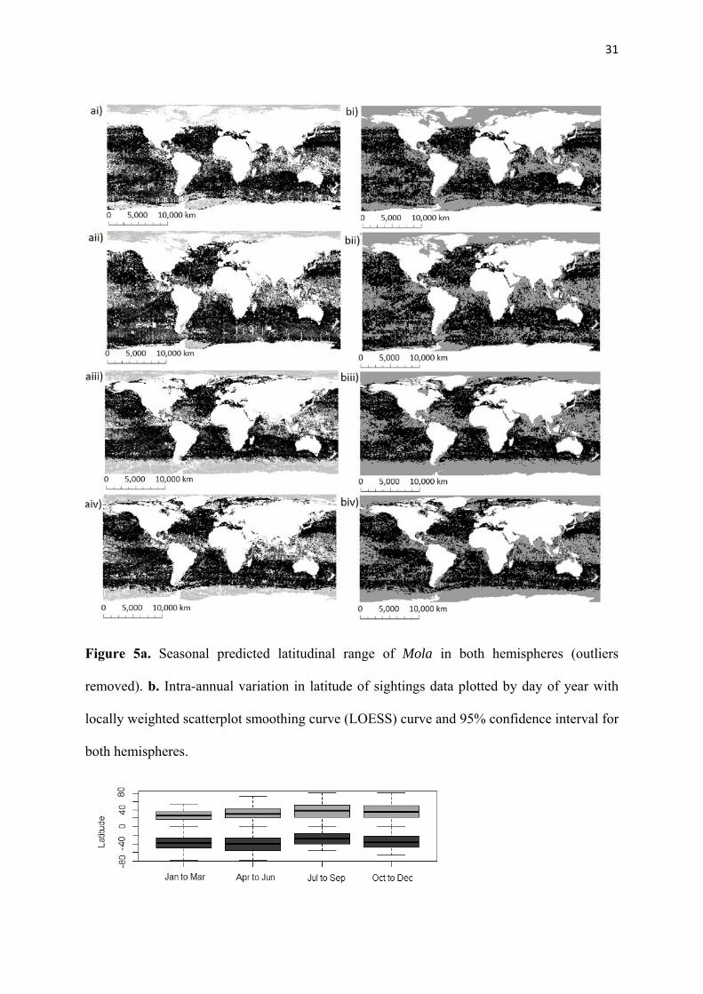
(Fig. 4a and b); but with lowest occurrence in polar and equatorial waters. The extent of 237 

suitable habitat (defined as the percentage suitable ocean surface) varied significantly 238 

between seasons (χ2df=3 = 591.2, p < 0.001; Table 3). The latitudinal range of Mola also 239 

varied significantly in both Northern (tested individually) across all seasons (χ2df=3 = 1690.5, 240 

tabulated χ2df=3 = 8.81e-11, p < 0.001) and Southern Hemispheres (χ2

df=3 = 3121.2, tabulated 241 

χ2df=3 = 8.81e-11, p < 0.001). Seasonal differences in latitudinal range reflected movement 242 

patterns, with the latitude of individual sightings varying temporally in both the Northern and 243 

Southern Hemispheres with animals shifting to more northerly latitudes in both hemispheres 244 

between April and October (Figs. 5a and b). 245 

246 

Discussion 247 

This study used detailed records from public sightings databases, alongside fisheries surveys 248 

and museum archives which provided global coverage of a Data Deficient genus (IUCN, 249 

2016). Although public sightings are widely used in broad-scale ecological studies, such data 250 

come with caveats, such as potential misidentification of cryptic species, incorrect data entry 251 

or regions of limited data availability. Despite such restrictions, such citizen science 252 

initiatives offer extensive coverage well beyond the budget and feasibility of most research 253 

projects. One of the best known examples, the North American Christmas Bird Count, has 254 

been running for over 100 years, with millions of person hours contributed to survey effort 255 

(Bibby, 2003; Audubon, 2008). With careful interpretation and strict data processing, 256 

substantial quantities of data can be collated over wide spatial and temporal scales, to the 257 

same quality as those collected by experts (Danielsen et al., 2014). 258 

12  

When applying SDM to sightings data, we must be aware of the limitations of the dataset in 259 

question, choose ecologically relevant variables (Mac Nally, 2000) and use appropriate 260 

methods (Elith & Leathwick, 2009). However, despite potential pitfalls and limitations, SDM 261 

have become important tools for predicting species distribution patterns and subsequent 262 

conservation management (Kremen et al., 2007; Wiens & Graham, 2005; Evans et al., 2015). 263 

In this study, SDM enabled us to delineate the range extent of ocean sunfishes, quantify 264 

distinct local clustering and describe seasonal changes in range extent accompanied with 265 

intra-annual movement patterns consistent with being a facultative seasonal migrant. 266 

267 

Distribution patterns 268 

To date, there are two recognised species within Mola: Mola mola (L. 1758) and Mola 269 

ramsayi (Giglioli, 1883). Alongside these two species, recent papers have reported 270 

differences between the Atlantic and Pacific M. mola populations based on genetic and 271 

morphological studies (e.g. Bass et al., 2005; Yoshita et al., 2009; Gaither et al., 2016). 272 

Despite these discoveries, a formal classification of cryptic species is yet to be published, and 273 

the species taxonomy of Mola remains in flux (see review by Pope, 2009). In light of the 274 

current pressures faced by the ocean sunfishes, this study provides baseline information on 275 

Mola spatial ecology, which can be further refined to species-specific level as discrepancies 276 

over speciation resolve themselves over time. 277 

Our study revealed that the genus Mola has a wide habitat range (see Fig. 1b) with confirmed 278 

sightings records extending 128° of latitude from approximately 70°N near Altenfjord, 279 

Norway to -58°S in the Beagle Canal, Chile (sightings contributed by Lukas Kubicek, pers. 280 

comm.). When compared to the latitudinal range extents of > 10 000 other marine species 281 

(Strona et al., 2012), this range would appear in the top 15 range extents (maximum reported 282 

range 150⁰ latitude). However, within this range, our analysis suggests that Mola frequently 283 

13  

aggregate and cluster in specific regions rather than being distributed randomly. Such 284 

clustering may be partly an artefact of sighting bias in coastal regions and known hotspots, 285 

particularly in North American and Europe. Nonetheless, the findings presented here align 286 

well with anecdotal evidence that Mola occur in patchily distributed, high density 287 

aggregations, particularly in coastal waters (e.g. Silvani et al., 1999; Sims & Southall, 2002; 288 

Houghton et al., 2006). 289 

Several regions globally have already been identified as hosting annual aggregations of Mola 290 

mola, suggested to be shoals of juveniles (< 1 m); for example in Camogli, Italy (Syväranta et 291 

al., 2012) and California, USA (Cartamil & Lowe, 2004; Thys et al., 2015), whilst our 292 

analysis may help predict other areas with high density populations. We are aware that 293 

limited data availability such as sparse information from equatorial regions, may have a 294 

partial effect on our habitat suitability predictions, but this is likely reduced by our 295 

implementation of a bias file. To the best of our knowledge, we have defined the full range 296 

extent of Mola (Fig. 1b), however, as sightings were likely subject to significant observer 297 

bias. Indeed, the predicted presence from SDMs (Fig. 4b) may be of greater use to 298 

characterise the actual range extent Mola populations whilst predicted probability values are 299 

likely correlated with density. 300 

301 

Environmental drivers of Mola distribution 302 

The Random Forest model provided the most reliable approximation of Mola distribution. 303 

Sea surface temperature and an indicator of regional productivity (chlorophyll a 304 

concentration) have been proposed as primary drivers of Mola movements (e.g. Thys et al., 305 

2015; Sims et al., 2009). Mola habitat suitability increased gradually with chlorophyll a 306 

concentration until reaching a threshold of approximately 140 mg m-3 with habitat suitability 307 

declining rapidly at higher concentrations. Many studies comment on Mola range limitation 308 

14  

in terms of minimum temperatures, and indeed we found sightings of Mola to be absent from 309 

waters below 7°C. However, our data suggested that Mola have a similarly-defined upper 310 

thermal threshold, of approximately 23°C, beyond which habitat suitability declined rapidly. 311 

In the Atlantic, M. mola were found to spend ~99% of their time in water temperatures 312 

between 10 - 19°C over a three month period (Sims et al., 2009), with a similar thermal 313 

preference of 16 - 17oC suggested from Pacific studies (Nakamura et al., 2015). The 314 

suggested thermal preference of approximately 16oC is further supported by our results, with 315 

habitat suitability peaking at this value. Interestingly, the warmest ambient water conditions 316 

recorded by external data loggers on free swimming M. mola, was 22°C (Nakamura et al., 317 

2015) with internal body temperatures ranging from 12 - 21°C; considerably narrower than 318 

external ambient water temperatures experienced by the fish (3 - 22°C). More recently, a 319 

study on spatial occupancy of tagged M. mola in the North East Atlantic suggested 320 

movements were strongly related to water temperature on regional scales with an “escape” 321 

from regional maxima of approx. 25°C (Sousa et al., 2016b). By combining such evidence 322 

alongside the modelled thermal response curves, we suggest that the genus Mola may have an 323 

upper thermal tolerance limit of approximately 23°C, although occasional forays above this 324 

temperature may occur as demonstrated by the recording of an individual M. ramsayi at a 325 

maximum of 27.5°C (Thys et al., 2016). Further support for a thermal optimum of 16°C can 326 

be derived from a recent study comparing optimum temperatures for performance in the wild 327 

to maximum temperature experiences in fish species’ ranges (Payne et al., 2016a). If a 328 

thermal optimum of 16°C is aligned with the expected response curve, then an upper thermal 329 

limit of 23°C would be expected from this genus (Payne et al., 2016b). The thermal limits 330 

identified in our study may, therefore, reflect a loss of performance beyond such limits, at a 331 

genus level, although further research will be required to confirm species specific responses. 332 

15  

From post-hoc analysis of the range extent of Mola, it appears that presence is also 333 

associated with dissolved oxygen levels between 5 and 7 ml/L. However, Thys et al. (2015) 334 

recently suggested that M. mola may be able to tolerate very low oxygen levels after 335 

observing individuals within ocean hypoxic zones at 60 m. Following periods exposed to 336 

such conditions, it is likely that individuals may need to recover in well-oxygenated waters 337 

(Cartamil & Lowe, 2004). To date, Mola mola and Mola ramsayi have been observed at 338 

maximum depths of 844 m (Potter & Howell, 2011) and 483 m respectively (Phillips et al., 339 

2015), suggesting that mesopelagic ranging of sunfishes is perhaps more common than 340 

previously thought (Phillips et al., 2015). However, although the Mola are capable of deep 341 

water ranging, large schools of small Mola spp. are often noted in coastal areas, possibly a 342 

reflection of their mixed diet at this life stage (e.g. Syväranta et al., 2012; Harrod et al., 2013; 343 

Nakamura & Sato, 2014). The increased availability of benthic prey and discards in coastal 344 

waters may function as a driver of seasonal abundance in shallow water in the genus Mola 345 

(Harrod et al., 2013). 346 

347 

Seasonal movements 348 

We identified large areas of suitable habitat available year-round for Mola, however, our 349 

results also suggested that the total suitable sea surface area and latitudinal position of varied 350 

significantly between seasons (see Fig. 5a). The predictive models (see Fig. 4) suggested that 351 

Mola thermal tolerance enables movement to higher latitudes in the Northern Hemisphere 352 

during the boreal spring to late summer, before retreating further south over the boreal 353 

autumn and winter months. Within the confines of this study, we were only able to model 354 

Mola presence in surface waters, however, these latitudinal movements may correspond to 355 

shifts in deep prey fields (Angel & Pugh, 2000; Houghton et al., 2008). Our predicted 356 

seasonal movement of Mola supports evidence from tagging studies in the northwest and 357 

16  

northeast Atlantic (e.g. Sims et al., 2009; Potter & Howell, 2011; Sousa et al., 2016b), and 358 

northeast and northwest Pacific (e.g. Dewar et al., 2010; Thys et al., 2015), which identified 359 

seasonal movements of individuals driven by temperature and patchily distributed prey. 360 

However, despite a range of tagging studies providing data across the Northern Hemisphere, 361 

there are relatively few data available from the Southern Hemisphere on Mola movements. 362 

From the SDMs, we suggest that a similar pattern occurs in the Southern Hemisphere, where 363 

Mola are able to move to maximum southern latitudes during the austral spring to late 364 

summer and then retreat towards the equatorial regions during the austral winter (Fig. 5a and 365 

b). These broad scale movements reflect the migration patterns of many species, in 366 

accordance with the seasonal migratory paradigm, where warmer temperatures during 367 

summer months enable range extensions poleward, and which then contract as the seasons 368 

change; example species include bluefin tuna (Lutcavage et al., 1999), swordfish (Sedberry et 369 

al., 2001) and loggerhead turtles (Mansfield et al., 2009). 370 

Our data suggest that although the average latitudinal position of Mola in surface waters 371 

varied over the seasons, much of the world’s oceans remain suitable for Mola year-round, 372 

with a wide latitudinal range. It is apparent, therefore, that Mola cannot be classified as 373 

obligate migrants, owing to discrepancies in distribution between populations. Although the 374 

species within this study were all considered to be Mola mola, the more common of the two 375 

Mola species, inferred differences in movement strategy between populations may be due to 376 

misidentification and behavioural differences between M. mola and the lesser studied M. 377 

ramsayi (Pope et al., 2010). Mola ramsayi is morphologically very similar to M. mola (Bass 378 

et al., 2005), identified by 16 fin rays with 12 closely spaced ossicles, compared to the 12 fin 379 

rays and 8 broadly spaced ossicles and reduced band of denticles prior to the clavus of M. 380 

mola (Fraser-Brunner, 1951; Thys et al., 2013). Mola ramsayi was initially suggested to be 381 

the Southern Hemisphere species (Fraser-Brunner, 1951), however, individuals have since 382 

17  

been identified in the Northern Hemisphere, including the Sea of Oman (Al Ghais, 1994), the 383 

Indian waters of Chennai (Mohan et al., 2006) and even co-occurring with M. mola (Bass et 384 

al., 2005). Further molecular genetic analyses are required to confirm species identification 385 

and to assess the movement ecology of these species (Pope et al., 2010). 386 

Alongside the predicted distribution patterns modelled here, the average position of Mola 387 

raw sightings was consistent with the concept of seasonal migration. However, outliers to this 388 

pattern do exist, supported by evidence of prolonged residency (e.g. Hays et al., 2009; Harrod 389 

et al., 2013). Since this study only assessed Mola surface distribution, it does not provide 390 

information on depth distribution, however several studies suggest that Mola spends a 391 

significant proportion of time (up to 30%) in surface waters less than 10 m deep (Potter & 392 

Howell, 2010). Although sightings data alone will be insufficient to fully determine the 393 

seasonal distribution patterns of marine species (Southall et al., 2005), the frequent sightings 394 

of Mola in surface waters is related to their universal basking behaviour at the sea surface 395 

(Norman & Fraser, 1938). We suggest that the surface prediction of Mola distribution will 396 

provide a useful measure of their global distribution. 397 

Although the results of this study do not provide direct evidence of a reciprocal migration, 398 

they do support the suggestion that some populations move latitudinally as suitable 399 

conditions shift over the course of the year. Such long distance movements may be restricted 400 

to populations near the latitudinal limits of their distribution; however, further study is 401 

required to test this assertion. Taken together, these results suggest that the genus Mola 402 

contains populations subject to differing drivers of distribution and, therefore, we propose 403 

they may be classed as facultative seasonal migrants. 404 

405 

Conclusions 406 

18  

This study provides a first assessment of the spatio-temporal global biogeography of the 407 

genus Mola. Taken together, our results suggest that the genus is globally distributed with 408 

significant clustering in specific locations, influenced by sea surface temperatures ranging 409 

from ~7 to 23°C. Based on SDMs, we suggest that populations act as facultative seasonal 410 

migrants with differing regional drivers of distribution. Although this study was able to 411 

consider the potential influence of productivity (using the proxy variable of chlorophyll 412 

concentration), future work may be able to assess smaller regions which have better data 413 

availability. Further studies on the ontogenetic shifts in the diet of ocean sunfishes are also 414 

required to integrate SDMs with international databases of putative prey items to explore the 415 

life history significance of shallow water and offshore habitats in more detail. 416 

417 

Acknowledgements 418 

The authors would like to acknowledge the generous contribution of all those who collected 419 

and provided data for this study (for full list please see Appendix S1), particularly the 420 

thousands of citizen scientists globally, without whom this work would not be possible. Many 421 

thanks also to Lawrence Eagling for proof-reading the manuscript on several occasions. 422 

N.D.P was funded by The Fisheries Society of the British Isles. 423 

19  

References 424 

Al-Ghais, S. (1994) A first record of Mola ramsayi (Osteichthyes: Molidae) for the United 425 

Arab Emirates. Tribulus, 4, 22. 426 

Allouche, O., Tsoar, A., Kadmon, R. (2006) Assessing the accuracy of species distribution 427 

models: prevalence, kappa and the true skill statistic (TSS). Journal of Appliped Ecology, 428 

43, 1223-1232. 429 

Altman, D.G. (1990) Practical statistics for medical research. Chapman and Hall, CRC Press 430 

London. 431 

Anderson, R.P. (2003). Real vs. artefactual absences in species distributions: tests for 432 

Oryzomys albigularis (Rodentia: Muridae) in Venezuela. Journal of Biogeography, 30, 433 

591–605. 434 

Angel M.V. & Pugh P.R. (2000) Quantification of diel vertical migration by macroplankton 435 

and micronektonic taxa in the northeast Atlantic. Hydrobiologia, 440, 161–179. 436 

Audubon (2008) Available at: http://www.audubon.org/Bird/cbc/. 437 

Baddeley A., Rubak E., & Turner R. (2015) Spatial Point Patterns: Methodology and 438 

Applications with R. 439 

Bass A.L., Dewar H., Thys T., Streelman J.T., & Karl S. a. (2005) Evolutionary divergence 440 

among lineages of the ocean sunfish family, Molidae (Tetraodontiformes). Marine 441 

Biology, 148, 405–414. 442 

Bibby C.J. (2003) Fifty years of Bird Study : Capsule Field ornithology is alive and well, and 443 

in the future can contribute much more in Britain and elsewhere. Bird Study, 50, 194–444 

210. 445 

Cartamil D.P. & Lowe C.G. (2004) Diel movement patterns of ocean sunfish Mola mola off 446 

southern California. Marine Ecology Progress Series, 266, 245–253. 447 

Danielsen F., Pirhofer-Walz K., Adrian T.P., Kapijimpanga D.R.K., Burgess N.D., Jensen 448 

20  

P.M., Bonney R., Funder M., Landa A., Levermann N., & Madsen J. (2014) Linking 449 

public participation in scientific research to the indicators and needs of international 450 

environmental agreements. Conservation Letters, 7, 12–24. 451 

Dobbyn P. (2015) Available at: http://www.ktuu.com/news/news/a-series-of-bizarre-fish-452 

sightings-reported-in-alaska/35733240. 453 

Elith J., Graham C., Anderson R., Dudik M., Ferrier S., Guisan A., Hijmans R., Huettmann 454 

F., Leathwick J., Lehmann A., Li J., Lohmann L., Loiselle B., Manion G., Moritz C., 455 

Nakamura M., Nakazawa Y., Overton J., Peterson A., Phillips S., Richardson K., 456 

Scachetti-Pereira R., Schapire R., Soberon J., Williams S., Wisz M., & Zimmermann N. 457 

(2006) Novel methods improve prediction of species’ distributions from occurrence 458 

data. Ecography, 29, 129–151. 459 

Elith J. & Leathwick J.R. (2009) Species Distribution Models: Ecological Explanation and 460 

Prediction Across Space and Time. Annual Review of Ecology, Evolution, and 461 

Systematics, 40, 677–697. 462 

Ferrier S., Biology S., & Apr N. (2002) Mapping Spatial Pattern in Biodiversity for Regional 463 

Conservation Planning : Where to from Here ? Mapping Spatial Pattern in Biodiversity 464 

for Regional Conservation Planning : Where to from Here ? 51, 331–363. 465 

Franklin J. (2009) Mapping species distributions: spatial inference and prediction. Board 466 

Member of Landscape Ecology Journal of Vegetation Science, 336. 467 

Fraser-Brunner A. (1951) The ocean sunfishes (Family Molidae). Bull Br Mus (Nat Hist) 468 

Zoo, 87–121. 469 

GBIF (2015) Available at: http://doi.org/10.15468/dl.q3wkgk. 470 

Harrod C., Syväranta J., Kubicek L., Cappanera V., & Houghton J.D.R. (2013) Reply to 471 

Logan & Dodge: “stable isotopes challenge the perception of ocean sunfish Mola mola 472 

as obligate jellyfish predators”. Journal of fish biology, 82, 10–6. 473 

21  

Hays G.C., Farquhar M.R., Luschi P., Teo S.L.H., & Thys T.M. (2009) Vertical niche 474 

overlap by two ocean giants with similar diets: Ocean sunfish and leatherback turtles. 475 

Journal of Experimental Marine Biology and Ecology, 370, 134–143. 476 

Houghton J.D.R., Cedras A., Myers A.E., Liebsch N., Metcalfe J.D., Mortimer J. a., & Hays 477 

G.C. (2008) Measuring the state of consciousness in a free-living diving sea turtle. 478 

Journal of Experimental Marine Biology and Ecology, 356, 115–120. 479 

Houghton J.D.R., Doyle T.K., Davenport J., & Hays G.C. (2006) The ocean sunfish Mola 480 

mola: insights into distribution, abundance and behaviour in the Irish and Celtic Seas. 481 

Journal of the Marine Biological Association of the UK, 86, 1237. 482 

IUCN (2016) Available at: http://www.iucnredlist.org/about/overview. 483 

Jing, L., Zapfe, G., Shao, K.-T., Leis, J.L., Matsuura, K., Hardy, G., Liu, M., Robertson, R. & 484 

Tyler J. (2010) Available at: http://www.iucnredlist.org/. 485 

Nakamura I., Goto Y., & Sato K. (2015) Ocean sunfish rewarm at the surface after deep 486 

excursions to forage for siphonophores. Journal of Animal Ecology, 84, 590–603. 487 

Nakamura I. & Sato K. (2014) Ontogenetic shift in foraging habit of ocean sunfish Mola 488 

mola from dietary and behavioral studies. Marine Biology, 161, 1263–1273. 489 

NASA (2003) Available at: 490 

http://neo.sci.gsfc.nasa.gov/view.php?datasetId=GEBCO_BATHY. 491 

NASA (2012) Available at: 492 

http://neo.sci.gsfc.nasa.gov/view.php?datasetId=MY1DMM_CHLORA. 493 

NOAA (2015) Available at: http://www.nodc.noaa.gov/OC5/woa13/woa13data.html. 494 

Payne N.L., Smith J.A., van der Meulen D.E., Taylor M.D., Watanabe Y.Y., Takahashi A., 495 

Marzullo T.A., Gray C.A., Cadiou G., & Suthers I.M. (2015) Temperature-dependence 496 

of fish performance in the wild: links with species biogeography and physiological 497 

thermal tolerance. Functional Ecology, . 498 

22  

Pearson R.G., Raxworthy C.J., Nakamura M., & Townsend Peterson A. (2007) Predicting 499 

species distributions from small numbers of occurrence records: A test case using 500 

cryptic geckos in Madagascar. Journal of Biogeography, 34, 102–117. 501 

Petersen S. & McDonell Z. (2007) A bycatch assessment of the Cape horse mackerel 502 

Trachurus trachurus capensis mid- water trawl fishery off South Africa. Birdlife/WWF 503 

Responsible Fisheries Programme Report 2002–2005, . 504 

Phillips N.D., Harrod C., Gates A.R., Thys T.M., & Houghton J.D.R. (2015) Seeking the sun 505 

in deep, dark places: Mesopelagic sightings of ocean sunfishes (Molidae). Journal of 506 

Fish Biology, 87, 1118–1126. 507 

Pope E.C., Hays G.C., Thys T.M., Doyle T.K., Sims D.W., Queiroz N., Hobson V.J., 508 

Kubicek L., & Houghton J.D.R. (2010) The biology and ecology of the ocean sunfish 509 

Mola mola: A review of current knowledge and future research perspectives. Reviews in 510 

Fish Biology and Fisheries, 20, 471–487. 511 

Potter I.F. & Howell W.H. (2011) Vertical movement and behavior of the ocean sunfish, 512 

Mola mola, in the northwest Atlantic. Journal of Experimental Marine Biology and 513 

Ecology, 396, 138–146. 514 

R Development Core Team (2008) R Development Core Team. . 515 

Ricklefs R.E. (2004) A comprehensive framework for global patterns in biodiversity. Ecology 516 

Letters, 7, 1–15. 517 

Rissler L.J. & Apodaca J.J. (2007) Adding more ecology into species delimitation: ecological 518 

niche models and phylogeography help define cryptic species in the black salamander 519 

(Aneides flavipunctatus). Systematic Biology, 56, 924–942. 520 

Rushton S.P., Merod S.J.O.R., & Kerby G. (2004) New paradigms for modelling species 521 

distributions? Journal of Applied Ecology, 41, 193–200. 522 

Silvani L., Gazo M., & Aguilar a. (1999) Spanish driftnet fishing and incidental catches in 523 

23  

the western Mediterranean. Biological Conservation, 90, 79–85. 524 

Sims D.W., Queiroz N., Doyle T.K., Houghton J.D.R., & Hays G.C. (2009) Satellite tracking 525 

of the World’s largest bony fish, the ocean sunfish (Mola mola L.) in the North East 526 

Atlantic. Journal of Experimental Marine Biology and Ecology, 370, 127–133. 527 

Sims D.W. & Southall E.J. (2002) Occurrence of ocean sun ¢ sh , Mola mola near fronts in 528 

the western English Channel. J. Mar. Biol. Ass. U.K, 82, 927–928. 529 

Sousa L.L., Queiroz N., Mucientes G., Humphries N.E., & Sims D.W. (2016) Environmental 530 

influence on the seasonal movements of satellite-tracked ocean sunfish Mola mola in the 531 

north-east Atlantic. Animal Biotelemetry, 4, 7. 532 

Syväranta J., Harrod C., Kubicek L., Cappanera V., & Houghton J.D.R. (2012) Stable 533 

isotopes challenge the perception of ocean sunfish Mola mola as obligate jellyfish 534 

predators. Journal of fish biology, 80, 225–31. 535 

Thuiller A.W., Georges D., Engler R., Georges M.D., & Thuiller C.W. (2015) Package 536 

“biomod2.” . 537 

Thys T.M., Ryan J.P., Dewar H., Perle C.R., Lyons K., O’Sullivan J., Farwell C., Howard 538 

M.J., Weng K.C., Lavaniegos B.E., Gaxiola-Castro G., Miranda Bojorquez L.E., Hazen 539 

E.L., & Bograd S.J. (2015) Ecology of the Ocean Sunfish, Mola mola, in the southern 540 

California Current System. Journal of Experimental Marine Biology and Ecology, 471, 541 

64–76. 542 

Supporting information 543 

Appendix S1 Data sources table of global sunfish sightings 544 

545 

Biosketch 546 

Natasha Phillips is a PhD researcher at the University of Belfast interested in the movement 547 

ecology, diet and energetics of ocean sunfishes (family Molidae). 548 

549 

24  

Editor and Handling Editor 550 

Michelle Gaither and Şerban Procheş 551 

552 

Author contributions: 553 

NDP, JDRH, TT, NR and CH conceived the ideas. TT and CM collected data. NDP and JH 554 

led the writing. HJW, SP, NR, NP advised on analysis. NDP analysed the data.555 

25  

Tables

Table 1. IUCN Red List designation for ocean sunfishes on both global and European scales.

IUCN Red Listing

Species Common name Global Scale European Scale

Mola mola (L. 1758) Ocean sunfish Vulnerable Data Deficient

Mola ramsayi (Giglioli 1883) Southern ocean sunfish Not Assessed Not Assessed

Masturus lanceolatus (Liénard 1840) Sharptail sunfish Least Concern Not Assessed

Ranzania laevis (Pennant 1776) Slender sunfish Least Concern Data Deficient

26  

Table 2. Evaluation metrics Kappa, true skill statistic (TSS) and receiver operating characteristic (ROC) values for all species distribution models (mean value of five model runs ± standard deviation). All models were performed in R, using package “Biomod2”.

SDM type Kappa Value TSS Value ROC Value Surface Range Envelope 0.14 ± 0.01 0.19 ± 0.02 0.60 ± 0.01 Classification Tree Analysis 0.42 ± 0.03 0.62 ± 0.08 0.83 ± 0.05 Random Forest 0.63 ± 0.04 0.72 ± 0.04 0.93 ± 0.02 Multiple Adaptive Regression Splines 0.36 ± 0.04 0.48 ± 0.07 0.81 ± 0.04 Flexible Discriminant Analysis 0.31 ± 0.03 0.41 ± 0.04 0.76 ± 0.05 Generalised Linear Model 0.25 ± 0.01 0.35 ± 0.05 0.71 ± 0.03 Generalised Additive Model 0.35 ± 0.05 0.45 ± 0.07 0.79 ± 0.04

   

27  

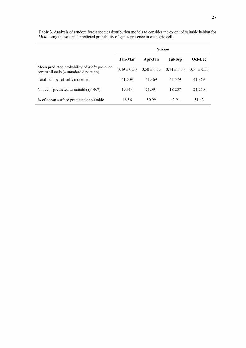
Table 3. Analysis of random forest species distribution models to consider the extent of suitable habitat for Mola using the seasonal predicted probability of genus presence in each grid cell.

Season

Jan-Mar Apr-Jun Jul-Sep Oct-Dec

Mean predicted probability of Mola presence across all cells (± standard deviation)

0.49 ± 0.50 0.50 ± 0.50 0.44 ± 0.50 0.51 ± 0.50

Total number of cells modelled 41,009 41,369 41,579 41,369

No. cells predicted as suitable (p>0.7) 19,914 21,094 18,257 21,270

% of ocean surface predicted as suitable 48.56 50.99 43.91 51.42

28  

Figures

Figure 1a. Global distribution of presence sightings of Mola (black) and pseudo-absences

provided by sightings of leatherback turtles (grey) used in the species distribution model. b.

Minimum convex hull range extent of Mola sightings data from 2000-2015. The origin of the

base map is a spheroid WGS 1984 projection.

29  

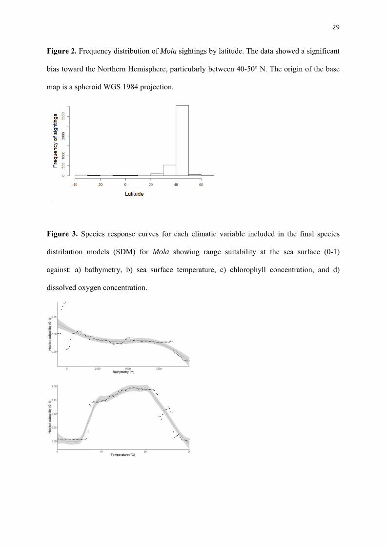
Figure 2. Frequency distribution of Mola sightings by latitude. The data showed a significant

bias toward the Northern Hemisphere, particularly between 40-50o N. The origin of the base

map is a spheroid WGS 1984 projection.

Figure 3. Species response curves for each climatic variable included in the final species

distribution models (SDM) for Mola showing range suitability at the sea surface (0-1)

against: a) bathymetry, b) sea surface temperature, c) chlorophyll concentration, and d)

dissolved oxygen concentration.

30  

Figure 4a. Seasonal range suitability at the sea surface for Mola from species distribution

model (SDM) outputs for i) January to March, ii) April to June, iii) July to September and iv)

October to December. Probability of presence shaded from 0 < 0.1 (white) to 0.9 < 1 (black)

at 0.1 intervals. b. predicted presence of Mola (probability >0.7). Predicted presence (black)

and predicted absence (grey). The origin of the base maps is a spheroid WGS 1984

projection.

31  

Figure 5a. Seasonal predicted latitudinal range of Mola in both hemispheres (outliers

removed). b. Intra-annual variation in latitude of sightings data plotted by day of year with

locally weighted scatterplot smoothing curve (LOESS) curve and 95% confidence interval for

both hemispheres.

32