Applications of machine learning for safe spillway discharge

Applications of machine learning for safe spillway discharge

Shicheng Li & James Yang

Department of Civil and Architectural Engineering

KTH Royal Institute of Technology

Contents

2021-10-06 2

• Introduction

• Research methods

• Example 1: Discharge determination

• Example 2: Aeration estimation

• Summary and future work

Introduction

2021-10-06 3

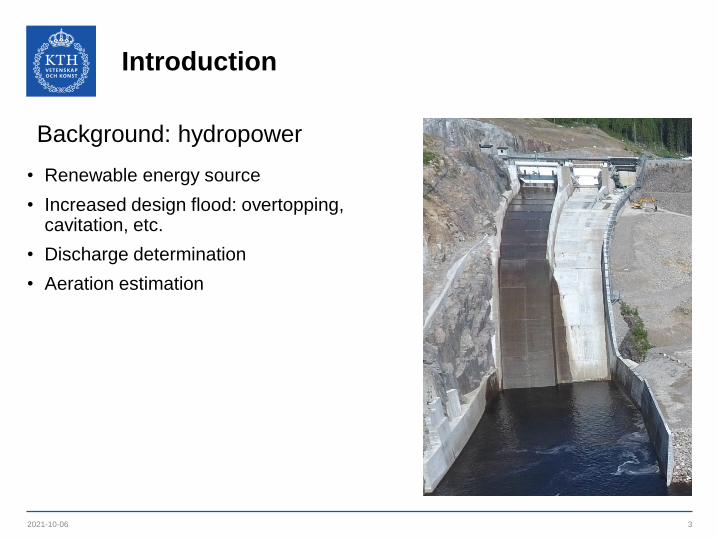
Background: hydropower

• Renewable energy source

• Increased design flood: overtopping, cavitation, etc.

• Discharge determination

• Aeration estimation

Introduction

2021-10-06 4

No. River name Dam name Z (m) Qo (m3/s) ∆ (%)

1

Umeälv

Ajaure 45 950 40

2 Stornorrfors 20 3300 35

3 Rusfors 22 1625 27

4Indalsälven

Midskog 27 2300 35

5 Bergeforsen 29 2300 45

6Ångermanälven

Stenkullafors 30 1250 40

7 Edensforsen 19 1400 >40

8 Skellefte älv Gallejaur 55 700 20

9 Klarälven Höljes 80 1600 >25

10Ljusnan

Långströmmen 28 1670 50

11 Halvfari 43 650 100

12

Lule älv

Letsi 85 1500 25

13 Porsi 40 2700 15

14 Vittjärv 15 2200 50

15 Boden 21 2800 20

Comparison of the old and new design floods: 20−50% increase

Research methods

2021-10-06 5

Conventional approaches

• Experimental test

• Numerical study (CFD)

• Field observation

Research methods

2021-10-06 6

Alternative method

• Machine learning

• Map feature data to labels

• Easily identifies trends and patterns

• Handling multi-dimensional and multi-variety data

• Continuous improvement

• Data acquisition

Advantages

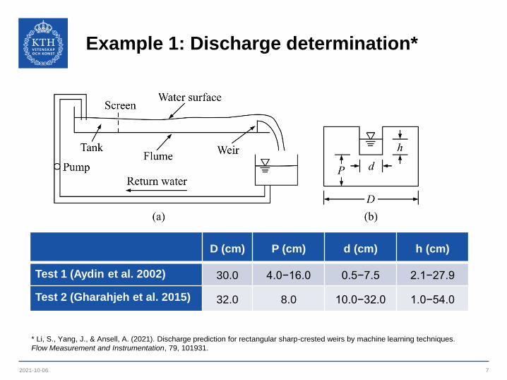
Example 1: Discharge determination*

2021-10-06 7

* Li, S., Yang, J., & Ansell, A. (2021). Discharge prediction for rectangular sharp-crested weirs by machine learning techniques.

Flow Measurement and Instrumentation, 79, 101931.

D (cm) P (cm) d (cm) h (cm)

Test 1 (Aydin et al. 2002) 30.0 4.0−16.0 0.5−7.5 2.1−27.9

Test 2 (Gharahjeh et al. 2015) 32.0 8.0 10.0−32.0 1.0−54.0

Example 1: Discharge determination

2021-10-06 8

Artificial neural network

1

1,2...,n

j i a i j ii

o f w x b j N


2021-10-06 9

• One hidden layer

• Randomly assigned weights in the input layer and analytically solved in the output layer

• Reduced risks of overfitting

Extreme learning machine


2021-10-06 10

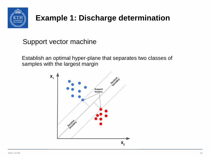
Establish an optimal hyper-plane that separates two classes of samples with the largest margin

Support vector machine


2021-10-06 11

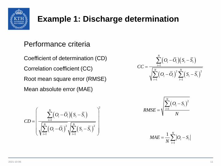
Performance criteria

2

1

2 2

1 1

N

i i i i

i

N N

i i i i

i i

O O S S

CD

O O S S

1

2 2

1 1

N

i i i i

i

N N

i i i i

i i

O O S S

CC

O O S S

2

1

N

i i

i

O S

RMSEN

1

1 N

i i

i

MAE O SN

Coefficient of determination (CD)

Correlation coefficient (CC)

Root mean square error (RMSE)

Mean absolute error (MAE)


2021-10-06 12

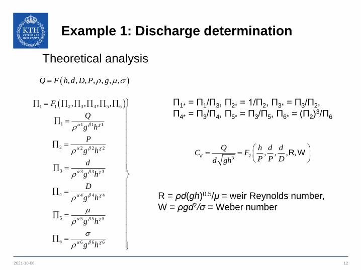
Theoretical analysis

, , , , , , ,Q F h d D P g

1 1 2 3 4 5 6

1 1 1 1

2 2 2 2

3 3 3 3

4 4 4 4

5 5 5 5

6 6 6 6

, , , ,

F

Q

g h

P

g h

d

g h

D

g h

g h

g h

Π1* = Π1/Π3, Π2* = 1/Π2, Π3* = Π3/Π2,

Π4* = Π3/Π4, Π5* = Π3/Π5, Π6* = (Π2)3/Π6

2

3, , , ,R W

d

Q h d dC F

P P Dd gh

R = ρd(gh)0.5/μ = weir Reynolds number,

W = ρgd2/σ = Weber number


2021-10-06 13

Input vectors

Input No.Dimensionless

parametersInput No.

Dimensionless

parameters

M1 h/D M6 h/P, d/P, R

M2 d/P M7 d/P, d/D, W

M3 h/P, d/D M8 h/P, d/P, d/D, R

M4 d/P, R M9 h/P, d/D, R, W

M5 h/P, d/P, d/D M10 h/P, d/P, d/D, R, W


2021-10-06 14

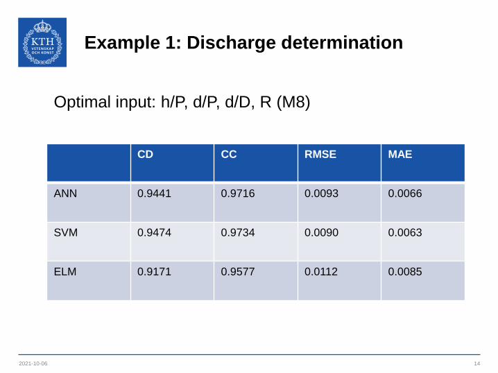
Optimal input: h/P, d/P, d/D, R (M8)

CD CC RMSE MAE

ANN 0.9441 0.9716 0.0093 0.0066

SVM 0.9474 0.9734 0.0090 0.0063

ELM 0.9171 0.9577 0.0112 0.0085


2021-10-06 15

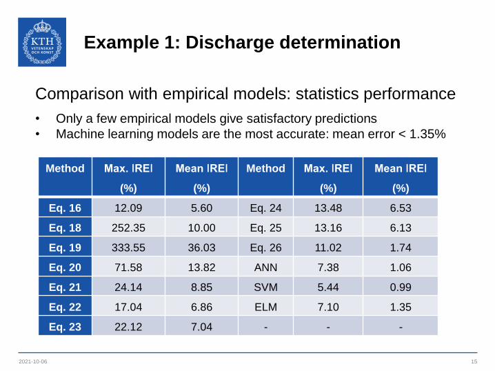
Comparison with empirical models: statistics performance

• Only a few empirical models give satisfactory predictions

• Machine learning models are the most accurate: mean error < 1.35%

Method Max. ǀREǀ

(%)

Mean ǀREǀ

(%)

Method Max. ǀREǀ

(%)

Mean ǀREǀ

(%)

Eq. 16 12.09 5.60 Eq. 24 13.48 6.53

Eq. 18 252.35 10.00 Eq. 25 13.16 6.13

Eq. 19 333.55 36.03 Eq. 26 11.02 1.74

Eq. 20 71.58 13.82 ANN 7.38 1.06

Eq. 21 24.14 8.85 SVM 5.44 0.99

Eq. 22 17.04 6.86 ELM 7.10 1.35

Eq. 23 22.12 7.04 - - -


2021-10-06 16

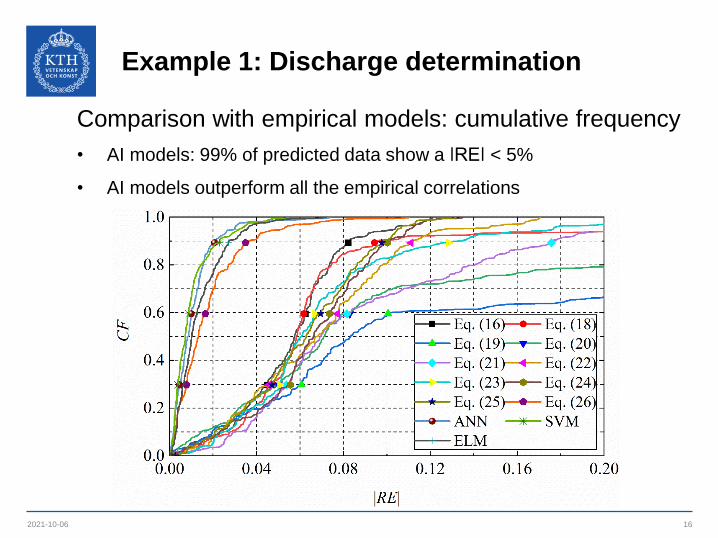
Comparison with empirical models: cumulative frequency

• AI models: 99% of predicted data show a ǀREǀ < 5%

• AI models outperform all the empirical correlations

Example 2: Aeration estimation*

2021-10-06 17

* Li, S., Yang, J., & Liu, W. (2021). Estimation of aerator air demand by an embedded multi-gene genetic programming. Journal of

Hydroinformatics, 23 (5): 1000–1013 .

1‒2% increase in air concentration

leads to 5‒7% reduction in cavitation

Example 2: Aeration estimation

2021-10-06 18

Multi-gene genetic programming

• Evolutionary based method

• Linear combination of low-depth GP trees

1 1 2 2 n nT c G c G c G b


2021-10-06 19

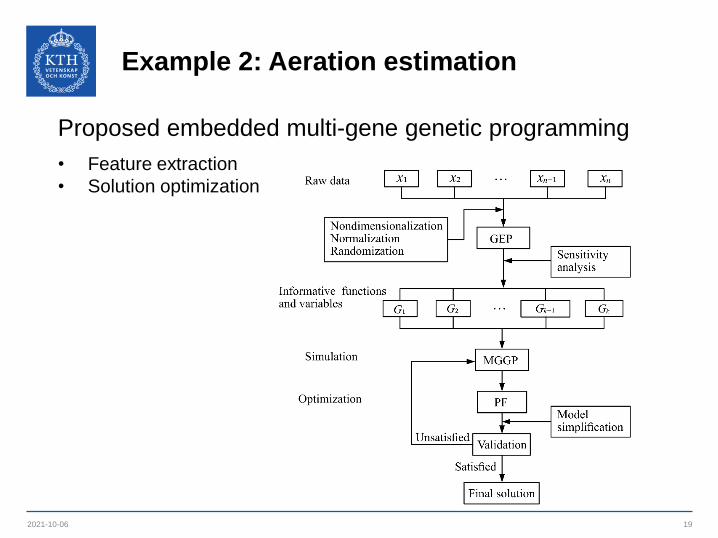
Proposed embedded multi-gene genetic programming

• Feature extraction

• Solution optimization


2021-10-06 20

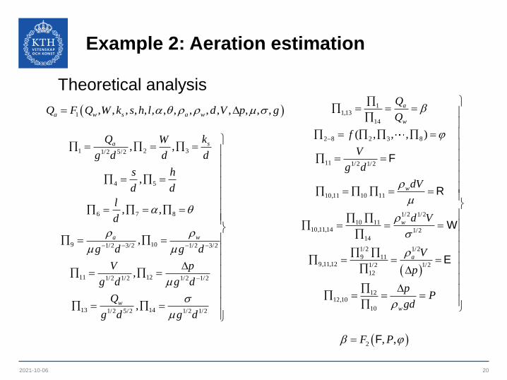
Theoretical analysis

1 , , , , , , , , , , , , , , ,a w s a wQ F Q W k s h l d V p g

1 2 31/2 5/2

4 5

6 7 8

9 101/2 3/2 1/2 3/2

11 121/2 1/2 1/2 1/2

13 141/2 5/2 1/2 1/2

, ,

,

, ,

,

,

,

a s

a w

w

Q kW

g d d d

s h

d d

l

d

g d g d

V p

g d g d

Q

g d g d

11,13

14

2 8 2 3 8

11 1/2 1/2

10,11 10 11

1/2 1/2

10 1110,11,14 1/2

14

1/2 1/2

9 119,11,12 1/21/2

12

1212,10

10

( , , , )

F

R

W

E

a

w

w

w

a

w

Q

Q

f

V

g d

dV

d V

V

p

pP

gd

2 , ,FF P


2021-10-06 21

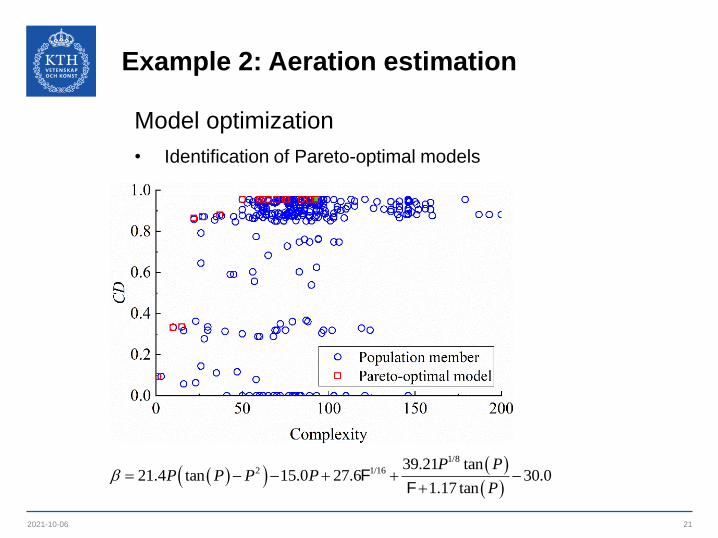
Model optimization

• Identification of Pareto-optimal models

1/8

2 1/1639.21 tan

21.4 tan 15.0 27.6 30.01.17 tan

FF

P PP P P P

P


2021-10-06 22

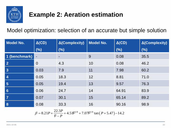
Model optimization: selection of an accurate but simple solution

Model No. Δ(CD)

(%)

Δ(Complexity)

(%)

Model No. Δ(CD)

(%)

Δ(Complexity)

(%)

1 (benchmark) - - 9 0.08 35.5

2 0 4.3 10 0.08 46.2

3 0.03 7.9 11 7.98 60.2

4 0.05 18.3 12 8.81 71.0

5 0.05 19.4 13 9.57 76.3

6 0.06 24.7 14 64.91 83.9

7 0.07 30.1 15 65.14 89.2

8 0.08 33.3 16 90.16 98.9

1/8 1/822.3

8.21 4.51 7.07 tan 5.47 14.2F FF

PP P

P


2021-10-06 23

Comparison of different methods

Method

Training Testing

CD NSCRMSE

(m3/s)

MAE

(m3/s)CD NSC

RMSE

(m3/s)

MAE

(m3/s)

MGGP 0.955 0.953 0.155 0.119 0.947 0.946 0.152 0.118

EMGGP 0.955 0.950 0.161 0.121 0.945 0.936 0.166 0.124

GP 0.933 0.931 0.188 0.155 0.931 0.923 0.178 0.144

MethodRecalibrated

CD NSC RMSE (m3/s) MAE (m3/s)

M1‒3 0.281 0.279 0.596 0.447

M4 0.261 0.253 0.607 0.439

M5 0.776 0.776 0.288 0.235

M6 0.163 0.163 0.642 0.491

MLR 0.759 0.759 0.345 0.271


2021-10-06 24

Comparison of different methods using Taylor diagram

• Simultaneously capture multiple efficiency metrics

• The closer to observation, the better

• EMGGP is the most accurate one


2021-10-06 25

EMGGP results

• In good agreement with experiments

Summary and future work

2021-10-06 26

Summary

• Multiple machine learning models are developed to determine

flow discharge and aeration efficiency

• Machine learning methods show superior performance over

experimental approaches

Future work

• Reservoir water level forecasts, time series modelling

• Deep learning, e.g. long short-term memory (LSTM) and nonlinear

autoregressive with external input (NARX)

2021-10-06 27

Li, S. & Yang, J. A hybrid gene expression programming model for discharge prediction.

Water Management, 2021 (in press)

Li, S., Yang, J., & Liu, W. Estimation of aerator air demand by an embedded multi-gene genetic programming.

Journal of Hydroinformatics, 2021, 23(5), 1000−1013.

Li, S., Yang, J., & Ansell, A. Discharge prediction for rectangular sharp-crested weirs by machine learning techniques.

Flow Measurement and Instrumentation, 2021, 79, 101931.

Applications of machine learning for safe spillway discharge

Documents

Transcript of Applications of machine learning for safe spillway discharge