Applications of Fault Detection in Vibrating Structures - … · Structural fault detection and...

October 2012

NASA/TM–2012-217779

Applications of Fault Detection in Vibrating

Structures

Kenneth W. Eure

Langley Research Center, Hampton, Virginia

Edward Hogge

Lockheed Martin, Hampton, Virginia

Cuong Chi Quach and Sixto L. Vazquez


Andrew Russell

Virginia Polytechnic Institute and State University, Blacksburg, Virginia

Boyd L. Hill

ViGYAN, Inc., Hampton, Virginia

https://ntrs.nasa.gov/search.jsp?R=20120016440 2018-07-14T20:47:22+00:00Z

NASA STI Program . . . in Profile

Since its founding, NASA has been dedicated to the

advancement of aeronautics and space science. The

NASA scientific and technical information (STI)

program plays a key part in helping NASA maintain

this important role.

The NASA STI program operates under the

auspices of the Agency Chief Information Officer.

It collects, organizes, provides for archiving, and

disseminates NASA’s STI. The NASA STI

program provides access to the NASA Aeronautics

and Space Database and its public interface, the

NASA Technical Report Server, thus providing one

of the largest collections of aeronautical and space

science STI in the world. Results are published in

both non-NASA channels and by NASA in the

NASA STI Report Series, which includes the

following report types:

TECHNICAL PUBLICATION. Reports of

completed research or a major significant phase

of research that present the results of NASA

Programs and include extensive data or

theoretical analysis. Includes compilations of

significant scientific and technical data and

information deemed to be of continuing

reference value. NASA counterpart of peer-

reviewed formal professional papers, but

having less stringent limitations on manuscript

length and extent of graphic presentations.

TECHNICAL MEMORANDUM. Scientific

and technical findings that are preliminary or of

specialized interest, e.g., quick release reports,

working papers, and bibliographies that contain

minimal annotation. Does not contain extensive

analysis.

CONTRACTOR REPORT. Scientific and

technical findings by NASA-sponsored

contractors and grantees.

CONFERENCE PUBLICATION.

Collected papers from scientific and

technical conferences, symposia, seminars,

or other meetings sponsored or co-

sponsored by NASA.

SPECIAL PUBLICATION. Scientific,

technical, or historical information from

NASA programs, projects, and missions,

often concerned with subjects having

substantial public interest.

TECHNICAL TRANSLATION.

English-language translations of foreign

scientific and technical material pertinent to

NASA’s mission.

Specialized services also include organizing

and publishing research results, distributing

specialized research announcements and feeds,

providing information desk and personal search

support, and enabling data exchange services.

For more information about the NASA STI

program, see the following:

Access the NASA STI program home page

at http://www.sti.nasa.gov

E-mail your question to [email protected]

Fax your question to the NASA STI

Information Desk at 443-757-5803

Phone the NASA STI Information Desk at

443-757-5802

Write to:

STI Information Desk

NASA Center for AeroSpace Information

7115 Standard Drive

Hanover, MD 21076-1320

http://www.sti.nasa.gov/

National Aeronautics and

Space Administration

Langley Research Center

Hampton, Virginia 23681-2199

October 2012

NASA/TM–2012-217779

Applications of Fault Detection in Vibrating

Structures

Kenneth W. Eure


Edward Hogge

Lockheed Martin, Hampton, Virginia

Cuong Chi Quach and Sixto L. Vazquez


Andrew Russell

Virginia Polytechnic Institute and State University, Blacksburg, Virginia

Boyd L. Hill

ViGYAN, Inc., Hampton, Virginia

Available from:

NASA Center for AeroSpace Information 7115 Standard Drive

Hanover, MD 21076-1320 443-757-5802

The use of trademarks or names of manufacturers in this report is for accurate reporting and does not constitute an official endorsement, either expressed or implied, of such products or manufacturers by the National Aeronautics and Space Administration.

Abstract

Structural fault detection and identification remains an area of active research. Solutions to

fault detection and identification, fdi, may be based on subtle changes in the time series history

of vibration signals originating from various sensor locations throughout the structure. The

purpose of this paper is to document the application of vibration based fault detection methods

applied to several structures. Overall, this paper demonstrates the utility of vibration based

methods for fault detection in a controlled laboratory setting and limitations of applying the same

methods to a similar structure during flight on an experimental subscale aircraft.

Introduction

Structural health monitoring may be achieved by characterizing the vibration frequency

response of structures under test and observing subtle changes in the frequency spectrum. This

paper examines several structures under test in a laboratory setting and within an unmanned

subscale aircraft. It is demonstrated that small changes in structural integrity may be detected

within a controlled laboratory setting while detection of similar structural faults proves difficult

during actual flight. The problem is to utilize existing signal processing methods to extract

statistical estimations of the probability of a structural fault based on sensor outputs such as

accelerometer and strain gauge outputs. The goal of this paper is to explore the use of spectral

based methods for structural fault detection. This paper is divided as follows. Section 1 consists

of an introduction to the theory, Section 2 presents simulation examples, Section 3 discuses the

experimental setup, Section 4 presents experimental results, and in Section 5 conclusions are

stated.

1. Review of Methods

The use of vibration based methods has been demonstrated for structural fault detection [1].

Vibration techniques offer the ability to track subtle changes in structural integrity based on

deviations in the structure’s frequency characteristics. This paper explores the possibility of

using structural vibration methods for in flight fault detection on an unmanned aerial vehicle.

Vibration based methods have historically been applied in a controlled laboratory setting with

reasonable results [1]. Several fault detection methods are explored in this paper using both

laboratory and in flight data. This section presents a review of the two detection methods used in

this paper.

1.1 Spectral Density, a non-parametric method

One technique used in this experiment for fdi requires at least one sensor mounted on the

structure at a location suitable for vibration detection. The resulting signal is analyzed for

spectral content and compared to a known “good” spectral density taken from a structure known

to have no faults. If the comparison is favorable, the structure is declared to be without fault.

However, an off comparison indicates a possible structural fault.

1

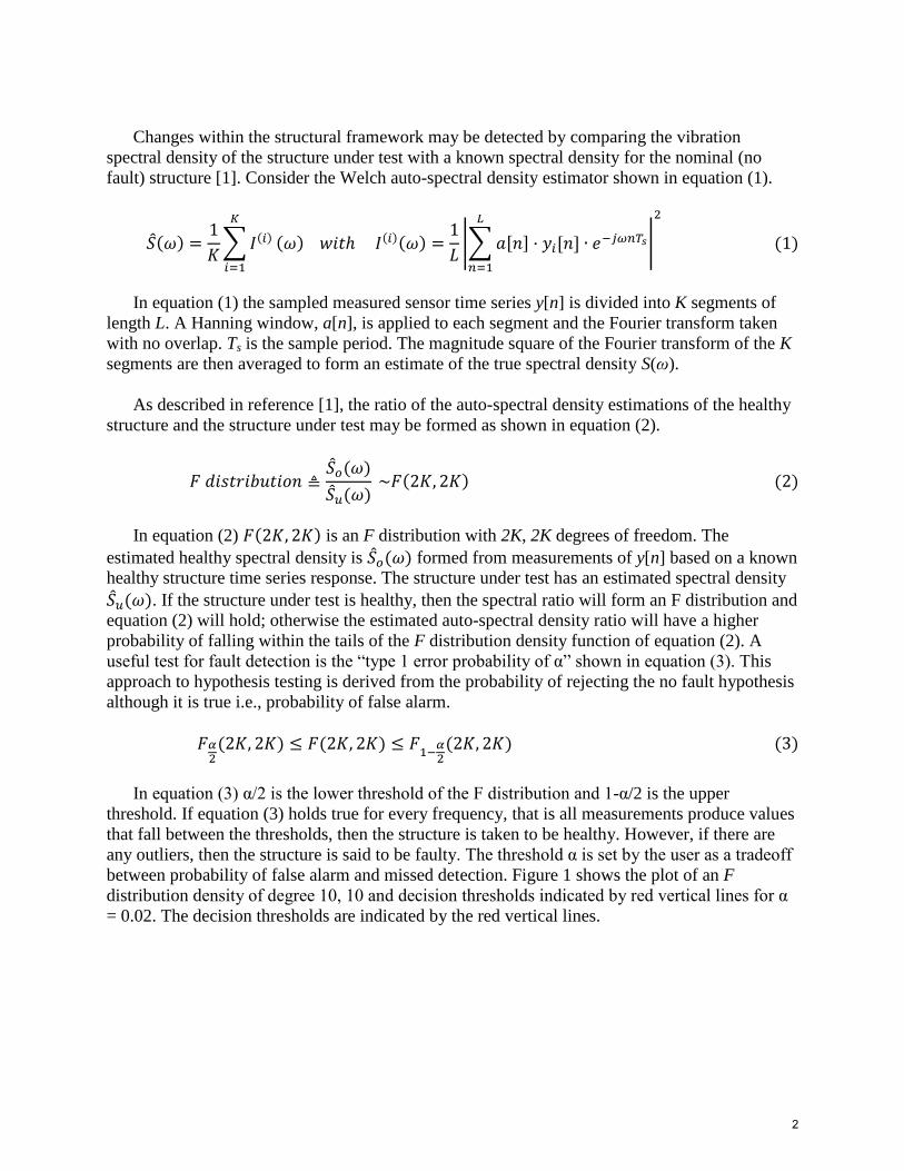
Changes within the structural framework may be detected by comparing the vibration

spectral density of the structure under test with a known spectral density for the nominal (no

fault) structure [1]. Consider the Welch auto-spectral density estimator shown in equation (1).

( )

∑ ( )

( ) ( )( )

|∑ [ ] [ ]

|

( )

In equation (1) the sampled measured sensor time series y[n] is divided into K segments of

length L. A Hanning window, a[n], is applied to each segment and the Fourier transform taken

with no overlap. Ts is the sample period. The magnitude square of the Fourier transform of the K

segments are then averaged to form an estimate of the true spectral density S(ω).

As described in reference [1], the ratio of the auto-spectral density estimations of the healthy

structure and the structure under test may be formed as shown in equation (2).

( )

( ) ( ) ( )

In equation (2) ( ) is an F distribution with 2K, 2K degrees of freedom. The

estimated healthy spectral density is ( ) formed from measurements of y[n] based on a known

healthy structure time series response. The structure under test has an estimated spectral density

( ). If the structure under test is healthy, then the spectral ratio will form an F distribution and

equation (2) will hold; otherwise the estimated auto-spectral density ratio will have a higher

probability of falling within the tails of the F distribution density function of equation (2). A

useful test for fault detection is the “type 1 error probability of α” shown in equation (3). This

approach to hypothesis testing is derived from the probability of rejecting the no fault hypothesis

although it is true i.e., probability of false alarm.

( ) ( )

( ) ( )

In equation (3) α/2 is the lower threshold of the F distribution and 1-α/2 is the upper

threshold. If equation (3) holds true for every frequency, that is all measurements produce values

that fall between the thresholds, then the structure is taken to be healthy. However, if there are

any outliers, then the structure is said to be faulty. The threshold α is set by the user as a tradeoff

between probability of false alarm and missed detection. Figure 1 shows the plot of an F

distribution density of degree 10, 10 and decision thresholds indicated by red vertical lines for α

= 0.02. The decision thresholds are indicated by the red vertical lines.

2

Figure 1: Illustration of F distribution with decision thresholds

Figure 1 was produced using the MATLAB commands fpdf and finv. If all values for F in

equation (2) for every frequency fall between the red vertical lines of Figure 1, the structure is

declared to be healthy. However, if a computed value falls outside the red lines, then a fault can

be declared with a probability of false alarm equal to α, in this case 0.02.

An advantage of using this technique is that it is simple and requires no knowledge of the

input excitation; only the output sensor signal is needed. A disadvantage is that it is more

susceptible to environmental disturbances such as wind and engine vibration noise. Other non-

parametric techniques include the frequency response function based method and the coherence

measure based method as described in reference [1].

1.2 Model Parameter Based Method, a parametric method

A second technique used here is a model parameter based method [1]. A system

identification technique is used to find the model parameters of the nominal system and an

estimate of the nominal covariance matrix. The unknown system under test is then modeled

using input/output data and the model parameters and the covariance matrix are estimated. In

order to achieve fault detection, a comparison is made between the identified nominal system’s

model parameters and the system’s covariance matrix as compared to that of the system under

test. Consider equation (4).

( )

0 0.5 1 1.5 2 2.5 3 3.5 4 4.5 50

0.1

0.2

0.3

0.4

0.5

0.6

0.7

0.8

Values of F(10,10)

F D

istr

ibution D

ensity F

unction

Healthy Structure Range

3

In equation (4) the nominal system’s model parameters and covariance matrix are and

respectively and that of the system under test are and . The parameters and are the

variances of the system excitation inputs typically taken to be or normalized as one. Equation (4)

may be used to form a quality test Q given in equation (5).

( )

The test variable Q forms a chi-square distribution with degree of freedom equal to the

number of estimated system parameters [1], and may be used for structural fault detection. If the

value falls to the left of a chosen cut off value as shown by the red line in Figure (2), the system

is declared good, however, if Q falls to the right, a fault is declared. As with the non-parametric

method, fault detection is based on the probability of false alarm.

Figure 2: Illustration of Chi-Square distribution with decision threshold

This method of fault detection offers increased immunity to environment disturbances but

requires more computations than the non-parametric method. Also, a measure of the excitation

signal may be required for this modeling method. However, if no excitation measure is available,

sensor signals may be used alone but at the cost of a loss of robustness to environmental

disturbances. For the applications used in this paper, the parameters chosen consist of the

Observer Markov parameters as shown in equation (6). The reader is referred to references [1, 2]

for more details concerning system modeling.

Healthy

Structure

4

2. Simulation Examples

In this section a second order system will be used to demonstrate the utility of both fault

detection methods. Consider equation (6).

( ) ( ) ( ) ( ) ( ) ( ) ( )

In equation (6) y(t) is the measured sensor response to the normally distributed zero mean,

unit variance input u(t). The coefficients and are chosen to represent a single vibration

mode and are given in Table 1.

Coefficient Nominal Case Damaged Case 1.2728 1.1690 -0.8100 -0.8100 0.5000 0.5000 0.7000 0.7000 1.2000 1.2000

ω (natural frequency) 0.7854 0.8640 1-σ (dampening) 0.9000 0.9000

Table 1: Coefficients of equation (6)

To demonstrate the nominal case, two independent time sequences of u(t) were applied to

equation (6) using the nominal case coefficients of Table 1 and the auto-spectral density of the

output y(t) was estimated for each using equation (1). In the spectral estimation process, a

Hamming window was used and the data y(t) of length 107 for each case was portioned into ten

non-overlapping segments (K=10). The ratio of the two spectral density estimates was taken as

given by equation (2). For this test case, both are considered known healthy structures. Since the

same system described by equation (6) using the nominal case coefficients was driven by two

independent sets of random inputs, equation (2) produces the F distribution shown in Figure 3.

As expected, the simulated case (blue) very closely follows an F distribution, (red). Figure 3 was

produced using the MATLAB commands pwelch, hist and fpdf.

5

Figure 3: Simulation example using known healthy structure

In order to test the method’s ability to detect faults, the second set of coefficients shown

in Table 1 were used and the resulting auto-spectrum divided into that produced by the nominal

coefficient set as in equation (2). The resulting distribution is shown in Figure 4 along with the F

distribution density curve for comparison.

0 1 2 3 4 5 60

0.1

0.2

0.3

0.4

0.5

0.6

0.7

0.8

0.9

1

Ratio of Spectral Densities

F D

istr

ibution D

ensity C

urv

e

simulated

theorectical

F(20,20)

6

Figure 4: Typical result for the damaged system, blue curve; and nominal, red curve

Nominal Case (ω=0.7854) Damaged Case (ω=0.8640)

F(min) F(max) F(min) F(max) 0.0995 8.6218 0.0670 13.0221 0.1009 10.9227 0.0823 15.4641 0.0737 10.7298 0.0666 14.9704 0.0829 9.4192 0.0625 12.7819 0.1062 7.8956 0.0727 16.7895 0.0920 9.3571 0.0639 14.7947 0.1076 8.9217 0.0794 15.5781 0.0984 9.9814 0.0486 14.8895 0.0859 12.3366 0.0918 14.3831 0.0764 11.4971 0.0860 15.8822

Table 2: Maximum and minimum F distribution values (Lower bound = 0.0802, Upper

bound = 12.4751)

Table 2 lists the maximum and minimum values of F obtained from ten simulations using the

nominal coefficients of Table 1 for the healthy case to produce the auto-spectrum estimate

( ), and the damaged case coefficients of Table 1 to produce the auto-spectrum estimate

( ). The data length was 107. The data were divided into ten non-overlapping segments (K =

10) and the auto-spectral density was estimated using the MATLAB command pwelch. After

forming the ratio as in equation (2), the MATLAB command hist was used to create the blue plot

of Figure 4; the red plot is the ideal F density distribution of degree 20, 20. As can be seen in this

plot along with Table 2, the alterations in the natural frequency of the damaged case can be

0 1 2 3 4 5 6 7 80

0.1

0.2

0.3

0.4

0.5

0.6

0.7

0.8

0.9

1

Values of F(10,10)

F D

istr

ibution D

ensity C

urv

e

Damaged Simulation

F Distribution Curve

7

detected most of the time. By examining the data in Table 2 a lower threshold of 0.0802 and an

upper threshold of 12.4751 will differentiate between the nominal and damaged cases for most

simulations with α set to 5x10-7

. One can use such a small probability of false alarm in this case

because of the large data size and the absence of external disturbances since this is an idealized

simulation. However, two false alarms did occur as indicated in red italics. Since 524,289

frequencies were tested ranging between 0 and π, it is reasonable that a few of the nominal case

values would fall on the tails of the F distribution thus creating a false alarm. Alternatively, the

probability of false alarms may be reduced at the expense of an increase in the probability of

missed detection by further reducing α.

In addition to demonstrating the use of the spectral technique to detect simulated damage, the

parametric technique may also be used. For these simulations, the form of equation (6) was

expanded to include a non-zero constant in order to eliminate the need of removing the direct

current, DC, component when the technique is applied to experimental data. This representation

is given in equation (7).

( ) ( ) ( ) ( ) ( ) ( ) ( )

The parameters in equation (7) are the same as in equation (6) with the additional parameter

DC that will be determined using system identification. In practice the value of DC will be

determined by the DC offset in the sensor, such as the offset in accelerometers or strain gauges.

The vector ones is simply a time series of ones. Figure 5 shows the simulation results using the

nominal system as given by the parameters of Table 1. As with the non-parametric technique, the

plot demonstrates that the simulation follows the expected theoretical distribution; for the

parametric technique a χ2 distribution is observed.

Figure 5: Simulation example using known healthy structure

8

In Figure 5 the red line is a plot of the chi-square probability density function and the blue

stars are simulation results. The simulation results were obtained from 105 iterations of a

simulation using 103 data points produced from equation (7). From equation (7) we see there are

six unknown parameters to be estimated, producing the six degree of freedom chi-square

distribution as expected. While Figure 5 was produced using the nominal system as both the

baseline and the system under test, Figure 6 was produced using the damaged system of Table 1

as the system under test. As can be seen from the blue stars generated using the damaged

simulation, clearly the damage was easily detected.

Figure 6: Typical result for the damaged system

In comparing Figures 4 and 6, it can be easily seen by the larger separation between the

nominal and damaged case distribution in Figure 6 compared to Figure 4 that the parametric

technique offers superior fault detection capability for this simulated case. However, this

increase in fault detection capability comes with the requirement that the excitation signal be

available for measure and at an increase in computational complexity.

3. Experimental Setups

The purpose of this section is to describe the experimental setups. Figure 7 shows the

laboratory experimental setup used to detect a mass located at the far edge of a vibrating panel.

This first laboratory experiment is relevant because it demonstrates the utility of the methods in a

9

simple test platform. In addition, an experiment was designed to detect a cut placed in the panel

stiffener as shown in Figure 8.

Figure 7: Experimental setup for structural fault detection.

The experimental setup consists of an aluminum plate mounted on a robotic shaker. The plate

is one-foot wide by four-feet long with one-inch aluminum stiffeners bolted to the perimeter.

Both the plate and stiffeners are 1/16 inch thick. As can be seen in Figure 7, the plate was

secured to the robot pedestal at one end and the other end is free. At the free end is an

accelerometer used to gather data for this experiment. The first two runs had no weight added to

the outboard panel edge. The next two runs had a 5g blue clay mass added as can be seen in

Figure 7. Two other mass values were used: 10g and 15g. All masses were added at the location

shown in Figure 7 and all data was taken from the outboard accelerometer located next to the

blue clay mass. The accelerometer located by the blue clay mass was glued to the edge of the

plate as shown and the clay mass stuck to the plate end without the need of an adhesive. The

other accelerometers shown in Figure 7 were not used for this experiment.

The input to the robotic shaker was band-limited white noise from 0 to 10 Hz. This

bandwidth was chosen because it was the highest frequency possible for reliable operation of the

robotic data system. The output data was measured using a computer with a sample rate of 200

Hz. The data was digitally filtered using an eighth order Butterworth filter with a cutoff

frequency of 20Hz. After filtering, the data was decimated by five. The resulting output covers

the frequency range from 0 to 20 Hz. The mean was subtracted to remove any DC component.

Table 3 summarizes the data used to detect the various test masses.

10

0g 5g 10g 15g

Set 1 Run 1 Run 1 Run 1 Run 1

Set 2 Run 2 Run 2 Run 2 Run 2

Table 3: Summary of test mass experimental data

In another experiment to simulate damage, several cuts were made in the aluminum stiffener

located on the perimeter of the plate. An example is shown in Figure 8.

Figure 8: Cut in plate aluminum stiffener

Figure 8 shows a 3 mm (~1/8 inch) cut on the right side of the plate stiffener. In order to

introduce various levels of damage and to test the ability of the vibration methods to detect the

damage, cuts were progressively made. The first cut was 3 mm on the right side followed by

deepening this cut to 7 mm. Next a second 3 mm cut was made on the left side. For each level of

damage, data was collected and processed as done previously using the test masses. Only the

parametric technique was applied to this experimental setup.

In addition to the vibrating panel of Figure 7, a cut aluminum tube which serves onboard the

EDGE aircraft was tested as shown in Figure 9. The EDGE aircraft, a Subscale Aerial Vehicle,

SAV, served as the final experimental platform for structural fault detection. The aluminum tube

shown in Figure 9 is the main structural support for the wings of the Edge aircraft shown in

Figure 10. In Figure 9 the tube under test is the shinny aluminum tube with the masses taped to

both ends and an accelerometer centrally located. The tube was mounted on the shaker and test

masses added to the tube as shown to simulate aerodynamic loading. Band-limited noise was

used to drive the shaker and an accelerometer located towards the tube end was used as the

output sensor. Data were taken for both the no cut case and a 3 mm cut case.

11

Figure 9: Aluminum tube used for crack detection

Figure 10: EDGE, left, and with wing support tube showing and wings removed, right

12

Figure 11: Locations of strain gauges, left, and accelerometers, right within EDGE aircraft

Several flights were performed with both the cut tube and the uncut tube in place in order to

demonstrate the application of structural fault techniques to detect the tube damage using

vibration techniques. This experiment differs from that of the robotic shaker in that no coherent

broad band noise source is present to excite the tube structure; rather the flight environment and

propeller noise are relied on to produce the vibrations for fault detection. Table 4 lists the flight

numbers along with the condition of the tube.

Undamaged Tube Tube with 3 mm cut

18, 19, 20, 21 22, 23, 24, 25

Table 4: List of flight numbers and tube condition

From Table 4 four flights were carried out with the uncut tube and four flights with the cut

tube. All flights consisted of various maneuvers such as take-off, turns with banks, and landing.

Data was gathered at a sampling rate of 500 Hz from the sensors located as described in Figure

11 throughout all flight maneuvers. The cut location is shown as a red line in the left Figure 11.

The red lines shown in the right Figure 11 are not cuts but divisions between the EDGE flaps and

ailerons. Details of the EDGE data acquisition system may be found in reference [3].

4. Experimental Results

This section presents the experimental results obtained from applying the detection

theory of Section 1 to the experimental setups of Section 3.

13

F D

istr

ibu

tion

Den

sity

Fun

ctio

n

4.1 Results using the spectral technique

Figure 12 shows the probability density distribution of F(2K,2K), equation (2) for the

nominal case of no added weight in Figure 7. The blue points result from experimental data

using the 0g runs in Table 3 while the red curve is the theoretical F distribution. The

experimental data was filtered with a Hanning window. No data overlap was used and the Welch

segmentation K was 40, resulting in an F distribution of degree 80, 80. The total data length was

28,000, and 1,001 frequency points were used for the auto-spectrum estimation. These points

were equally distributed between 0 and π. As was expected, the comparison of two nominal

cases shown by the set of blue points (Run 1 with Run 2, 0g column) closely follows the

theoretical prediction curve in red.

Figure 12: Plot of density function comparing two nominal 0g cases

Using the two no weight cases as standards for the nominal system to produce two sets of

( ), the ratio of the auto-spectral densities of the weighted cases, ( ), and the no weight

cases were compared for damage detection as given by equation (2). The results are shown in

Table 5.

( )/ ( ) 5g 10g 15g

0g Run 1 with weighted Run 1 0.4995, 1.9929 0.3363, 2.9625 0.1769, 4.6918




Table 5: Fault detection using 0g base lines with 0.4740 and 2.1095 detection thresholds

0 0.5 1 1.5 2 2.5 3 0

0.2

0.4

0.6

0.8

1

1.2

1.4

1.6

2

F(2K,2K)

1.8

14

The minimum and maximum values of equation (2) may be used to set a detection threshold

by computing the ratio of the two 0g cases. Two minima and two maxima result; one from taking

the spectral ratio of run 1 to run 2, the other from taking the spectral ratio of run 2 to run 1. These

values are 0.5176, 0.5377 for the minima and 1.8597, 1.9321 for the maxima. In Table 5 the first

row lists the weights used in the experiment. The second row lists the minimum and maximum

values produced by equation (2) when the first 0g case was used as the nominal case to produce

( ) and the first set of data using the weights was used to produce ( ). Row three repeats

row two except the second set of data obtained for the weighted panel is used to produce ( ). Likewise, rows four and five repeat the analysis using the second ( ). The choice of α will set

the detection threshold. The detection threshold is a balance between missed detection and false

alarm. A risk level is chosen as 0.001 resulting in lower and upper decision thresholds of 0.4740

and 2.1095 respectively. When these values are applied to Table 5 both the 10g and 15g weights

can be easily detected. However, detection of the 5g weight fails in one comparison as can be

seen in the second row in red italics. Here, we see that the maximum and minimum values are

within the set detection threshold although the 5g mass is present.

4.2 Experimental results using the parametric technique

The purpose of this section is to tabulate results obtained using the parametric method of

fault detection. Table 6 summarizes the results obtained by adding 5 and 10g masses to the panel

of Figure 7. Runs beyond those listed in Table 3 were performed for the 0g case to establish a

better statistical base. Each entry in Table 6 is the computed Q value. The first seven rows and

columns compare all 0g cases to one another. The data in the red italics compares the 0g cases

with the 5g cases. The data in the blue gothic font compares the 0g with the 10g cases. The data

in purple antique font compares the 5g cases with the 10g cases. As can be seen, all black data

values are less than any of the colored data values, thus showing the ability of the parametric

technique to differentiate between cases of different added masses.

Run # 1 (0g) 2 (0g) 3 (0g) 4 (0g) 5 (0g) 6 (0g) 7 (0g) 8 (5g) 9 (5g) 10 (10g) 11 (10g)

1 (0g) 0.00 5.85 4.45 20.26 22.15 4.02 4.93 51.24 61.88 116.63 117.67

2 (0g) 5.85 0.00 8.89 22.49 25.52 7.40 6.07 75.37 89.43 162.50 162.67

3 (0g) 4.45 8.89 0.00 33.78 39.15 5.68 5.28 94.90 116.51 184.99 185.86

4 (0g) 20.26 22.49 33.78 0.00 2.95 29.37 20.41 58.25 65.97 159.00 157.97

5 (0g) 22.15 25.52 39.15 2.95 0.00 33.39 23.92 59.16 67.10 168.43 171.37

6 (0g) 4.02 7.40 5.68 29.37 33.39 0.00 5.41 70.20 81.41 162.11 165.69

7 (0g) 4.93 6.07 5.28 20.41 23.92 5.41 0.00 72.79 80.03 150.76 148.21

8 (5g) 51.24 75.37 94.90 58.25 59.16 70.20 72.79 0.00 3.30 45.34 51.58

9 (5g) 61.88 89.43 116.51 65.97 67.10 81.41 80.03 3.30 0.00 58.40 67.97

10 (10g) 116.63 162.50 184.99 159.00 168.43 162.11 150.76 45.34 58.40 0.00 3.02

11 (10g) 117.67 162.67 185.86 157.97 171.37 165.69 148.21 51.58 67.97 3.02 0.00

Table 6: Detection of 5 and 10 gram masses using parametric technique: 1-7 are 0 grams; 8-9

are 5 grams, 10-11 are 10 grams. A 12th

order system I.D. was used

15

As can be seen when comparing the non-parametric lab results with those of the parametric

technique, the latter offered a performance advantage in the added-mass trials. In the next set of

experiments no masses were added and the stiffener was cut to induce damage, only the

parametric technique will be used. Tables 7 through 9 consider the fault detection cases of

various cuts as shown in Figure 8. In all cases, the black data represents comparisons of like

cases; that is, no cut compared to no cut, 3 mm cut compared with 3 mm cut, etc. The data shown

in red italics represents cross comparisons and should always be greater than the black data for

fault detection. Fault detection was achieved in all cases of Table 8; that is, the largest black

number Q is smaller than any red italic number. However, the data shown in Table 7

demonstrates the failure of the parametric technique to detect the 3 mm cut in the panel. The

extent of this failure may be seen by noticing that several of the back numbers are larger than the

smallest red italic, and that several of the red italic numbers are smaller than the largest black.

One possible explanation for this is that the 3 mm cut was insufficient to create a system level

change in the vibration characteristics of the panel. That is, the damage effect was limited to the

proximity of the 3 mm cut. Also, Table 9 demonstrates fault detection occurred around 80% of

the time when comparing a panel that was cut 7 mm on one side and 0 mm on the other with a 7

mm stiffener cut on one side and 3 mm on the other. Again, this may be due to the limited

damage range of the 3 mm cut.

Run

# 1 2 3 4 5 6 7 8 9 10 11 12 13 14 15 16

1 0.00 5.85 4.45 20.26 22.15 4.02 4.93 5.23 4.03 5.18 5.40 4.98 5.29 4.34 5.52 4.96

2 5.85 0.00 8.89 22.49 25.52 7.40 6.07 9.07 7.03 8.78 9.97 7.67 10.63 8.90 10.90 10.29

3 4.45 8.89 0.00 33.78 39.15 5.68 5.28 17.62 13.08 20.11 16.19 15.93 16.11 12.16 18.21 12.55

4 20.26 22.49 33.78 0.00 2.95 29.37 20.41 35.12 23.68 29.28 25.69 28.05 28.90 23.91 30.88 25.57

5 22.15 25.52 39.15 2.95 0.00 33.39 23.92 38.02 25.30 32.74 27.39 29.83 31.02 24.68 32.56 27.17

6 4.02 7.40 5.68 29.37 33.39 0.00 5.41 8.90 7.26 10.38 7.96 8.24 9.35 5.77 9.31 7.69

7 4.93 6.07 5.28 20.41 23.92 5.41 0.00 12.33 10.40 11.59 10.95 11.11 12.47 10.04 13.33 11.76

8 5.23 9.07 17.62 35.12 38.02 8.90 12.33 0.00 2.10 3.61 4.96 3.30 3.69 3.76 4.09 4.01

9 4.03 7.03 13.08 23.68 25.30 7.26 10.40 2.10 0.00 2.08 3.47 2.52 4.06 2.75 3.29 3.26

10 5.18 8.78 20.11 29.28 32.74 10.38 11.59 3.61 2.08 0.00 5.58 4.50 4.37 3.53 5.04 3.87

11 5.40 9.97 16.19 25.69 27.39 7.96 10.95 4.96 3.47 5.58 0.00 2.12 2.47 2.13 2.30 2.14

12 4.98 7.67 15.93 28.05 29.83 8.24 11.11 3.30 2.52 4.50 2.12 0.00 2.89 2.99 2.82 2.73

13 5.29 10.63 16.11 28.90 31.02 9.35 12.47 3.69 4.06 4.37 2.47 2.89 0.00 3.16 2.63 1.69

14 4.34 8.90 12.16 23.91 24.68 5.77 10.04 3.76 2.75 3.53 2.13 2.99 3.16 0.00 3.13 2.28

15 5.52 10.90 18.21 30.88 32.56 9.31 13.33 4.09 3.29 5.04 2.30 2.82 2.63 3.13 0.00 1.76

16 4.96 10.29 12.55 25.57 27.17 7.69 11.76 4.01 3.26 3.87 2.14 2.73 1.69 2.28 1.76 0.00

Table 7: Detection of 3 mm cut vs. no cut using parametric technique: 1-7 are no cut cases;

8-16 are 3 mm cuts, left side. 12th

order system I.D. was used.

16

Run

# 1 2 3 4 5 6 7 8 9 10 11 12 13 14 15

1 0.00 2.10 3.61 4.96 3.30 3.69 3.76 4.09 4.01 39.58 47.15 35.03 42.36 34.85 42.81

2 2.10 0.00 2.08 3.47 2.52 4.06 2.75 3.29 3.26 35.05 40.70 31.73 39.57 31.39 40.95

3 3.61 2.08 0.00 5.58 4.50 4.37 3.53 5.04 3.87 46.46 54.67 40.32 49.53 41.34 48.83

4 4.96 3.47 5.58 0.00 2.12 2.47 2.13 2.30 2.14 32.89 36.78 29.25 35.94 29.17 37.51

5 3.30 2.52 4.50 2.12 0.00 2.89 2.99 2.82 2.73 37.10 43.42 32.23 39.39 32.39 40.19

6 3.69 4.06 4.37 2.47 2.89 0.00 3.16 2.63 1.69 38.84 43.90 34.69 42.95 34.91 43.93

7 3.76 2.75 3.53 2.13 2.99 3.16 0.00 3.13 2.28 35.79 39.48 32.34 40.08 32.05 42.02

8 4.09 3.29 5.04 2.30 2.82 2.63 3.13 0.00 1.76 33.47 38.76 29.45 37.32 29.51 38.60

9 4.01 3.26 3.87 2.14 2.73 1.69 2.28 1.76 0.00 32.09 35.91 28.85 35.32 29.14 37.59

10 39.58 35.05 46.46 32.89 37.10 38.84 35.79 33.47 32.09 0.00 3.11 3.32 3.78 2.62 4.13

11 47.15 40.70 54.67 36.78 43.42 43.90 39.48 38.76 35.91 3.11 0.00 3.03 3.19 2.11 4.53

12 35.03 31.73 40.32 29.25 32.23 34.69 32.34 29.45 28.85 3.32 3.03 0.00 2.92 3.59 4.10

13 42.36 39.57 49.53 35.94 39.39 42.95 40.08 37.32 35.32 3.78 3.19 2.92 0.00 3.36 3.71

14 34.85 31.39 41.34 29.17 32.39 34.91 32.05 29.51 29.14 2.62 2.11 3.59 3.36 0.00 2.64

15 42.81 40.95 48.83 37.51 40.19 43.93 42.02 38.60 37.59 4.13 4.53 4.10 3.71 2.64 0.00

Table 8: Detection of 3 mm cut vs. 7 mm cut using parametric technique: 1-9 are 3 mm; 10-

15 are 7 mm. 12th


Run

#

1 2 3 4 5 6 7 8 9 10 11 12 13 14

1 0.00 3.11 3.32 3.78 2.62 4.13 6.46 9.31 7.95 6.07 4.80 6.92 8.55 8.36

2 3.11 0.00 3.03 3.19 2.11 4.53 9.36 12.01 11.15 7.51 5.80 9.95 10.19 10.22

3 3.32 3.03 0.00 2.92 3.59 4.10 8.93 14.06 12.42 10.02 7.64 11.13 12.63 12.34

4 3.78 3.19 2.92 0.00 3.36 3.71 8.21 12.82 11.29 8.19 5.70 11.27 10.03 10.06

5 2.62 2.11 3.59 3.36 0.00 2.64 5.47 6.74 6.00 4.43 3.41 5.32 7.33 6.75

6 4.13 4.53 4.10 3.71 2.64 0.00 6.28 9.03 8.01 6.54 3.96 7.82 9.12 8.57

7 6.46 9.36 8.93 8.21 5.47 6.28 0.00 3.90 5.81 4.13 4.63 3.66 3.91 2.74

8 9.31 12.01 14.06 12.82 6.74 9.03 3.90 0.00 4.27 4.24 4.74 3.48 5.37 2.25

9 7.95 11.15 12.42 11.29 6.00 8.01 5.81 4.27 0.00 1.68 2.18 2.91 5.97 4.39

10 6.07 7.51 10.02 8.19 4.43 6.54 4.13 4.24 1.68 0.00 1.33 2.46 4.40 3.65

11 4.80 5.80 7.64 5.70 3.41 3.96 4.63 4.74 2.18 1.33 0.00 2.79 3.03 3.86

12 6.92 9.95 11.13 11.27 5.32 7.82 3.66 3.48 2.91 2.46 2.79 0.00 4.37 3.13

13 8.55 10.19 12.63 10.03 7.33 9.12 3.91 5.37 5.97 4.40 3.03 4.37 0.00 2.87

14 8.36 10.22 12.34 10.06 6.75 8.57 2.74 2.25 4.39 3.65 3.86 3.13 2.87 0.00

Table 9: Detection of right 7mm, left 3 mm cut vs. right 7 mm, left 0 mm cut using

parametric technique: 1-6 are right 7 mm, left 0 mm cut; 7-14 are right 7 mm, left 3 mm cut. 12th


The tube shown in Figure 9 was used as a test platform in preparation for aircraft structural

fault detection based on flight data. Only the parametric test was performed here. A comparison

of several of the uncut and cut cases resulted in Figure 13. In Figure 13 the solid blue curve

represents the theoretical distribution obtained while comparing the uncut cases. The green

asterisks result from a comparison of uncut tube data and the light blue asterisks result when

comparing the cut cases to one another. As expected, there was a positive comparison when

equation (5) was applied to like cases. However, when cross comparing the system parameters of

the cut with the uncut case as shown with the red asterisks, a clear indication of fault occurred in

all experimental test cases.

17

Figure 13: Plot of results for the aluminum tube

As a final application for structural fault detection using the parametric technique, equation

(5) was used in an attempt to detect the tube cut by post processing data obtained during flight.

The inputs were chosen as the center tube accelerometer (see Figure 11) and an accelerometer

located on the propeller motor mount. The output was taken off the left tube strain gauge, S4 in

Figure 11. A tenth order system model was used with a DC offset term. No post processing

filtering was performed. A Table of Q values generated from equation (5) is shown in Table 10.

Section A: Comparison of uncut tube with uncut tube; like comparison therefore small Q expected

Flight # 19 20 21

18 25.4397 15.6947 17.0942 -

19 - 32.8794 33.0005 -

20 - - 10.5057 -

Section B: Comparison of uncut tube with cut tube; unlike comparison, larger Q expected

Flight # 22 23 24 25

18 37.6237 44.5893 51.3930 29.0202

19 48.5705 84.8742 70.1420 23.3063

20 38.1174 32.5272 35.3984 22.4707

21 40.1001 20.0700 22.0843 18.5254

Section C: Comparison of cut tube with cut tube; like comparison, small Q expected

Flight # 23 24 25 -

22 37.0281 48.1155 32.6480 -

23 - 16.0396 41.1743 -

24 - - 35.8340 -

Table 10: Values of Q with left tube strain as the system output and center tube

accelerometer and motor mount accelerometer as inputs.

18

In accordance to theory, the Q values should be spread around the number of parameters in

the system identification model, which for this case was thirty. As shown in Figure 2 fault

detection may be achieved by setting a threshold and declaring all values less than that threshold

to be without fault. From Table 10 Section A, we see that the values are for the most part smaller

than those given in Section B. This shows that the aircraft vibration response has changed

slightly between the flight numbers with Section B indicating a slightly larger miss compare than

that of Section A. This larger miss compare might indicate that the fault has been detected.

However, Section C also contains slightly larger numbers than Section A. Since the flights of

Section C were performed comparing the cut tube to the same cut tube, one would expect a more

favorable comparison; that is, the numbers were expected to be closer to those of Section A.

The data in Section B does indicate a greater miss-compare between the cut and uncut tube

flight cases when compared with the nominal uncut tube in most flight cases. This statistical

comparison does show that the system has changed after cutting the tube in comparison to before

the cut was made. However, it does not show what created the slight change. There are several

options: the environmental conditions (since the cut and uncut tube flights were performed on

different days), the cut in the tube, and/or the system changes resulting from pulling the wing off

to cut the tube. One cannot be sure of the overall increase in Q seen in Section B. It is suspected

that all three factors played a role. The change in environmental conditions played a role due to

the fact that flights were performed at different times spread across a three day period. Also,

different flight maneuvers were performed for each flight, creating different structural stresses

for each flight. All of these factors would come to play during real aircraft flight. The cut in the

tube also played a role by altering the vibration and stress loading of the tube. Also, perhaps

pulling the wing to cut the tube played a role in creating a system change. In the laboratory

experiments it was found that any slight change in the experimental setup created a substantial

change in the computed Q. For this reason all laboratory experiments were performed without

disassembling any of the system components between runs. It is suspected that just the act of

removing the wing to cut the tube and reattaching it can create a noticeable change in the system,

perhaps greater than the 3mm cut itself.

As an additional approach to fault detection, the strain versus acceleration may be compared

for the damaged and undamaged cases. Figure 14 shows this comparison for all flight cases.

Here no signal processing was done other than a simple average. The figure was generated with

the average of the raw sensor measurements for each case and the flight numbers shown are

those of Table 4. The acceleration signal was read from the left tube accelerometer of Figure 11

and the strain was taken from S4 of Figure 11.

19

Figure 14: Plot of average values for each flight case

From Figure 14 it can be seen that an overall difference in the strain for a given acceleration

in the vertical direction was observed between the cut (red line) and the uncut, (blue line) tube.

Both strain and acceleration are not calibrated and therefore only relative. That the cut tube

exhibits less strain for a given acceleration is to be expected due to the weaker connection

between the wing and aircraft frame. However, this may not necessarily be the case since other

factors such as removing and reattaching the wing and different environmental conditions could

easily account for the observations. Also, when other sensor values were compared, such as other

left wing strains versus accelerations, the pattern reported in Figure 14 was not consistent in the

data.

5. Conclusions

Several vibration fault detection methods were applied to a vibrating plate, aluminum tube,

and subscale aircraft in order to detect structural damage. The methods followed the theoretical

predictions and demonstrated utility in detecting various faults in a controlled laboratory setting.

This paper demonstrates that structural fault detection can be achieved using vibration methods

under controlled experimental conditions. The application of vibration based methods to actual

flight remains unclear. The flight experimental results obtained from the parametric method used

here are ambiguous. It is recommended that further flight experimentation be carried out using a

coherent source as an input to the flight structure under test. An input signal from a device such

as a piezoelectric transducer would produce a traceable coherent input thereby avoiding the need

to rely on environment inputs for parameter identification and fault detection.

20

1 Fassois, Spilios D., and John S. Sakellariou, “Time-series methods for fault detection and identification in

vibrating structures”, Philosophical Transactions of the Royale Society, 2007.

2 Klein, Vladislav, and Eugene A. Morelli, “Aircraft System Identification, Theory and Practice”, AIAA

Education Series, 2006.

3 Edward F. Hogge, “A Data System for a Rapid Evaluation Class of Subscale Aerial Vehicle”, NASA/TM–

2011-217145, May 2011.

21

REPORT DOCUMENTATION PAGE Form ApprovedOMB No. 0704-0188

2. REPORT TYPE Technical Memorandum

4. TITLE AND SUBTITLE

Applications of Fault Detection in Vibrating Structures

5a. CONTRACT NUMBER

6. AUTHOR(S)

Eure, Kenneth, W.; Hogge, Edward F.; Quach, Cuong Chi; Vazquez, Sixto L.; Russell, Andrew; Hill, Boyd, L.

7. PERFORMING ORGANIZATION NAME(S) AND ADDRESS(ES)NASA Langley Research CenterHampton, VA 23681-2199

9. SPONSORING/MONITORING AGENCY NAME(S) AND ADDRESS(ES)National Aeronautics and Space AdministrationWashington, DC 20546-0001

8. PERFORMING ORGANIZATION REPORT NUMBER

L-20186

10. SPONSOR/MONITOR'S ACRONYM(S)

NASA

13. SUPPLEMENTARY NOTES

12. DISTRIBUTION/AVAILABILITY STATEMENTUnclassified - UnlimitedSubject Category 39Availability: NASA CASI (443) 757-5802

19a. NAME OF RESPONSIBLE PERSON

STI Help Desk (email: [email protected])

14. ABSTRACT

Structural fault detection and identification remains an area of active research. Solutions to fault detection and identificationmay be based on subtle changes in the time series history of vibration signals originating from various sensor locations throughout the structure. The purpose of this paper is to document the application of vibration based fault detection methods applied to several structures. Overall, this paper demonstrates the utility of vibration based methods for fault detection in acontrolled laboratory setting and limitations of applying the same methods to a similar structure during flight on an experimental subscale aircraft.

15. SUBJECT TERMS

Fault detection; Spectral methods; Structures; Vibration18. NUMBER OF PAGES

2619b. TELEPHONE NUMBER (Include area code)

(443) 757-5802

a. REPORT

U

c. THIS PAGE

U

b. ABSTRACT

U

17. LIMITATION OF ABSTRACT

UU

Prescribed by ANSI Std. Z39.18Standard Form 298 (Rev. 8-98)

3. DATES COVERED (From - To)

5b. GRANT NUMBER

5c. PROGRAM ELEMENT NUMBER

5d. PROJECT NUMBER

5e. TASK NUMBER

5f. WORK UNIT NUMBER

534723.02.05.07

11. SPONSOR/MONITOR'S REPORT NUMBER(S)

NASA/TM-2012-217779

16. SECURITY CLASSIFICATION OF:

The public reporting burden for this collection of information is estimated to average 1 hour per response, including the time for reviewing instructions, searching existing data sources, gathering and maintaining the data needed, and completing and reviewing the collection of information. Send comments regarding this burden estimate or any other aspect of this collection of information, including suggestions for reducing this burden, to Department of Defense, Washington Headquarters Services, Directorate for Information Operations and Reports (0704-0188), 1215 Jefferson Davis Highway, Suite 1204, Arlington, VA 22202-4302. Respondents should be aware that notwithstanding any other provision of law, no person shall be subject to any penalty for failing to comply with a collection of information if it does not display a currently valid OMB control number.PLEASE DO NOT RETURN YOUR FORM TO THE ABOVE ADDRESS.

1. REPORT DATE (DD-MM-YYYY)10 - 201201-

Applications of Fault Detection in Vibrating Structures - … · Structural fault detection and...

Documents

Transcript of Applications of Fault Detection in Vibrating Structures - … · Structural fault detection and...