Applied Mathematical Modelling 35 (2011) 807–816

Contents lists available at ScienceDirect

Applied Mathematical Modelling

journal homepage: www.elsevier .com/locate /apm

Application of time reverse modeling on ultrasonic non-destructivetesting of concrete

Erik H. Saenger a,b,*, Georg Karl Kocur c, Roman Jud d, Manuel Torrilhon d

a Geological Institute, ETH Zurich, Zurich, Switzerlandb Spectraseis AG, Giessereistrasse 5, 8005 Zurich, Switzerlandc Institute of Structural Engineering, ETH Zurich, Zurich, Switzerlandd Seminar for Applied Mathematics, ETH Zurich, Zurich, Switzerland

a r t i c l e i n f o

Article history:Received 10 July 2009Received in revised form 16 July 2010Accepted 16 July 2010Available online 27 July 2010

Keywords:Time reverse modelingImagingFinite-differencesWave propagationSource localizationNon-destructive testing

0307-904X/$ - see front matter � 2010 Elsevier Incdoi:10.1016/j.apm.2010.07.035

* Corresponding author at: Geological Institute, EE-mail addresses: erik.saenger@erdw.ethz.ch (E

math.ethz.ch (M. Torrilhon).

a b s t r a c t

Time reverse modeling (TRM) is applied to localize and characterize acoustic emissionusing a numerical concrete model. Aim is to transform a method within exploration geo-physics to non-destructive testing. In contrast to previous time reverse applications, no sin-gle event or first onset time identification is applied. The method is described from amathematical point of view. So-called source TRM with limited knowledge of boundaryvalues is compared with so-called full TRM where a complete set of boundary conditionsis used. The resulting localization accuracy of both approaches is similar. With a knownthree-dimensional analytical solution we demonstrate the applicability and the limitationsof the two-dimensional wave propagation method solving the elastodynamic wave equa-tion. With the help of CT images we are able to digitalize a concrete specimen and to verifya used numerical concrete model. TRM localization using this highly scattering material isfeasible using the rotated staggered finite-difference method. We demonstrate the locali-zation of acoustic emission with a limited number of sensors and using effective elasticproperties. Source characteristics can also be recovered. Goal is to apply our method toacoustic emissions measured during experiments carried out on concrete and reinforcedconcrete specimen.

� 2010 Elsevier Inc. All rights reserved.

1. Introduction

Time reverse modeling (TRM) is applied in several fields of science such as medical and earth sciences [1]. Prior timereverse studies focus on filtering single events out of recordings of low signal to noise (S/N)-ratio [2] or on spatial andtemporal accuracy of single event localization [3]. We want to transfer a TRM approach within exploration geophysics toapplications within the field of non-destructive testing (NDT). The fundamental problem is to identify a source locationby solving the elastodynamic wave equation with limited data recorded at the boundaries of the modeling domain. However,those inversion problems are often ill-posed. We discuss application limitations and solution strategies.

Steiner et al. [4] applied TRM of the recorded surface wave field to better understand the passive low-frequency seismicwave field around hydrocarbon reservoirs and to determine whether some of the low-frequency signals originate fromhydrocarbon reservoirs. The TRM methodology uses numerical algorithms for two-dimensional elastic wave propagationin combination with an imaging condition. This imaging condition is implemented because the measured low-frequency

. All rights reserved.

TH Zurich, Zurich, Switzerland..H. Saenger), kocur@ibk.baug.ethz.ch (G.K. Kocur), roman.jud@math.ethz.ch (R. Jud), matorril@-

808 E.H. Saenger et al. / Applied Mathematical Modelling 35 (2011) 807–816

tremor signals were more or less continuous in time and no individual events or first arrival times could be detected. DuringTRM emitted seismic energy is propagated back to its origin. The seismograms recorded with synchronized three-componentseismometers are reversed in time and implemented as sources for numerical wave extrapolation. The signals are propa-gated backwards through the velocity model. The backward propagated energy will focus at the source location, if the veloc-ity model is accurate [3,4].

Concrete as a strongly heterogeneous and densely packed composite material represents a very important but also verydifficult object for ultrasonic NDT methods. Due to the high density of scattering constituents and inclusions, ultrasonic wavepropagation in this material consists of a complex mixture of multiple scattering, mode conversion and diffusive energytransport [5]. For a better understanding of the effect of aggregates, porosity and of crack distribution on elastic wave prop-agation in concrete and to optimize inverse reconstruction techniques, e.g. Impact echo methods [6], it is useful to simulatethe wave propagation and scattering process explicitly in the time domain [7–9].

Acoustic emissions (AE) are caused by strain energy release due to irreversible processes such as cracking or internal fric-tion in the material considered. Acoustic emission analysis (AEA) has become a promising method to evaluate the conditionof concrete structures [10,11]. Qualitative procedures make use of basic parameters of recorded signals and try to identifythe stage of degradation and to estimate the load history. Quantitative procedures attempt to identify characteristics ofan AE source and therefore have to consider the wave propagation between source and sensors. Profiting from the methodsof geophysics, considerable results have been achieved with respect to determination of onset times (picking), source local-ization and moment tensor analysis. Further progress depends on the handling of different crack distributions and crackedconcrete itself as the medium for elastic wave propagation, considering also other elements of structural concrete such asreinforcement bars and prestressing tendons.

The paper aims at establishing a tool for localization and further evaluation of acoustic emissions in structural concreteand shall contribute to better understanding on the relation between crack growth and AE activity. Concrete pervaded bycracks serves as a medium for elastic wave propagation and shall be observed, described, interpreted and modeled. The pro-cedure includes physical tests, to record and visualize crack formation and to obtain real AE data. Numerical forward mod-eling is used to evaluate and understand the physical tests. In this paper a feasibility study on a numerical concrete specimenis performed for this planned approach.

The challenging aspect for us is to transfer the time reverse modeling localization procedure by Steiner et al. [4] (de-scribed above) from geophysical exploration to the field of non-destructive testing in order to image acoustic emissionsoccurring during crack nucleation and growth in concrete. With TRM, receivers located like those in the physical modelare considered as sources in the numerical simulation. AE are traced back in time, and the location of the generating fractureprocess will become visible as a concentration of elastic energy. Advantages of this method are the independency of detec-tion/picking algorithms, the capability to handle low signal to noise ratios, and a possible identification of the moment tensorof the AE sources.

In the first part of the paper we briefly review the TRM approach by Steiner et al. [4]. In addition we perform a numericalaccuracy test based on a 3D analytical solution. For the second part we generate a 2D numerical concrete model and deter-mine the corresponding effective elastic properties. This allows a 2D plain strain feasibility study on the applicability of TRMin non-destructive testing. We conclude the paper with an outlook to 3D applications using real AE data.

2. Time reverse modeling of waves

In practise TRM is based on signals obtained from experiments which are send back into a specimen as sources in a timereverse manner. In this paper we investigate the potential of the TRM approach using a computational framework. Thismeans that a forward simulation is used to produce signals with full control of their origin. The forward computation is typ-ically based on an excitation localized in space and time. The waves emitted from this excitation are simulated up to a certainend time, while displacement values are recorded at specific boundary-points over time. These time-dependent values serveas signals in subsequent TRM simulations. Some mathematical details are described in this section. More details can befound in the work of Fink [12].

The computations of this paper are based on the linear anisotropic elastic wave equation for the displacement fielduiðx; tÞ 2 Rd (d = 2 in this paper) which reads:

qg ottui ¼ oj cijkl oluk� �

þ fi in X� ½0; T�: ð1Þ

The spatial domain of interest is denoted by X � Rd with positions x 2X and we consider time t 2 [0,T] with some end timeT. We use index notation for vectors and tensors with summation convention and oi ¼̂ o=oxi. In general, the equation featuresan inhomogeneity fi(x,t), which represents a space and time-dependent body force. The gravitational density is given by qg(x)and cijkl(x) denotes the stiffness tensor, which gives the momentum tensor by mij = cijkloluk. The equation contains no damp-ing term, such that it is form-invariant with respect to time-inversion transformation t ´ �t. For more information about themodeling, see for example [13]. Initial conditions are required for ui and the velocity otui, while boundary conditions can be ofDirichlet or Neumann type for ui.

The aim of TRM is to solve an inverse problem for the wave equation approximately. Note, that it is not the task to find aspatial and/or temporal distribution of a body force from boundary recordings, which is an ill-posed problem in general.

E.H. Saenger et al. / Applied Mathematical Modelling 35 (2011) 807–816 809

Instead the basis is an essentially homogeneous wave equation and the aim is to reconstruct a localized initial condition forthe displacement field from recorded boundary values. We distinguish between two different TRM procedures: source timereverse modeling (source TRM) and full time reverse modeling (full TRM). An overview about these procedures is displayedin Fig. 1.

2.1. Forward computation

A standard forward computation based on (1) is utilized to produce boundary signals which enter TRM simulations. Inthis paper we always apply the so-called rotated staggered finite-difference scheme to discretize the wave equation. For adescription of the numerical method see [14,15].

In our forward computations the initial displacement and velocity are not directly initialized but generated in the firsttime steps by a body force. Hence, the initial conditions are set to zero both for ui and its velocity, while the body force ischosen to be:

fiðx; tÞ ¼Riðx; tÞ t 2 ½0; ts�;0 t > ts;

�ð2Þ

which vanishes for time t > ts with a start-up time ts� T. Typically, Ri is chosen localized in space around a position xs with aspecific excitation pattern for example a second derivative of a Gaussian. After time ts a localized non-vanishing displace-ment field is generated which can be considered as actual initial condition emitting waves towards the boundaries. To imple-ment a free surface on the boundary of X Neumann conditions for ui are used. The aim of the TRM simulation below is to findan approximation to the original source position xs.

2.2. Source time reverse modeling

During a forward computation values of displacement are recorded by receivers on the boundary oX of the specimen. Thelocations of the receivers are denoted by

S ¼ xð1Þ;xð2Þ; . . . ; xðNÞ� �

� oX; ð3Þ

where N is the total number of source positions. In the following we will typically use N = 12. The time series of the displace-ment at position x(k) is written:

uðkÞi ðtÞ ¼ ui xðkÞ; t� �

; ð4Þ

with time t 2 [0,T]. These time series serve as input data for a TRM simulation. The position arrangement can be varied toevaluate the reproduction ability of the TRM simulation.

The TRM simulation is again based on the wave Eq. (1) using the same coefficients from the forward computation as wellas x 2X and t 2 [0,T]. No body force is present throughout the computation, fi = 0. Initial conditions for ui and otui are van-ishing, such that the equation is driven by boundary conditions. On oX the recorded signals uðkÞi are fed as sources into thedomain. Formally, we write:

uiðx; tÞ ¼ uðkÞi ðT � tÞ for x 2 S � oX ð5Þuiðx; tÞ ¼ 0 for x 2 oX n S; ð6Þ

such that inhomogeneous Dirichlet data is given exclusively in the source locations S. Note, that the time series is fed into thecomputation backwards in time. Hence, the TRM simulation reverses the forward computation.

The term source TRM emphasizes the way the time signals are implemented in the algorithm, i.e. as sources of waveexcitations. source TRM is not complete by definition in the sense that the equation is provided with time-reversed recei-

Fig. 1. A forward simulation of elastic wave propagation is used to generate synthetic input data for full and source TRM.

810 E.H. Saenger et al. / Applied Mathematical Modelling 35 (2011) 807–816

ver-signals at every boundary-point. Only a few selected points are used. In brief, we do not provide the equation with thefull set of information. It turns out that only a few boundary-points have to be provided with time-reversed signals toachieve very good results. Note that the source TRM has also been applied successfully to real models, i.e. using receiver data(representing the forward simulation) to carry out a numerical time reverse simulation in order locate a real physical waveexciting source. Such a real data example within exploration geophysics can be found in [4].

In the numerical method the actual domain X is supplemented by a layer of almost vacuum with zero Dirichlet conditionsat the outer computational boundary as described above. Hence, the time signals uðkÞi are inserted inside the numerical gridon the boundary grid points oX of the medium specimen. To avoid scattering they are superimposed to any existing values atthese grid points that are the results of interior and surface waves. By this technique the signals are interpreted as time seriesof localized initial conditions whose evolutions are superimposed in a time-delayed manner.

The waves emitted from the boundary sources during a source TRM simulation will interfere constructively in the dis-placement field and the location of strongest interference is taken as an approximation of the source location xs of the ori-ginal initial condition. In order to easily display the result of this interference in a TRM simulation we introduce the so-calledTRM-field defined by

TRMðxÞ :¼maxt2½0;T�

uiðx; tÞk k; ð7Þ

for every point x 2X. This means, in order to image the convergent wave focusing on the initial source, we store the max-imum particle displacement for each grid point throughout the entire time of modeling. The highest value of the TRM-fieldfinally makes it possible to locate the original source location, i.e. the source location of the forward simulation.

2.3. Full time reverse modeling

Due to time invariance an initial condition for a homogeneous wave equation can be exactly recovered in a time-reversedcomputation from the time series of all boundary values for times t 2 [0,T] and the displacement field and its velocity at timeT. An approximation to the initial conditions can be found when only the displacement field uðfwdÞ

i ðx; TÞ and its velocityotu

ðfwdÞi ðx; TÞ at time T are given from a forward simulation but no knowledge of the boundary values is available.For such a time reverse simulation we feed in the final fields as initial conditions:

uiðx; t ¼ 0Þ ¼ uðfwdÞi x; Tð Þ in X; ð8Þ

otuiðx; t ¼ 0Þ ¼ �otuðfwdÞi ðx; TÞ in X; ð9Þ

where the velocity is taken negative in correspondence to the time reversal. Since the numerical method is based on a two-step time integrator, see [14], such a reversed computation is easy to realize from the last two displacement fields at time Tand T � Dt. Both fields are simply used as initial fields for the two-step integrator in a reversed order. Boundary conditionsare the same as in the forward computation.

The result of such a full TRM simulation can be viewed as benchmark for a source TRM since much more information isused and typically the localization of the initial excitation is much better, see the example in the next section. However, fullTRM is typically not usable in practice due to the lack of knowledge in realistic situations.

2.4. Example for comparison

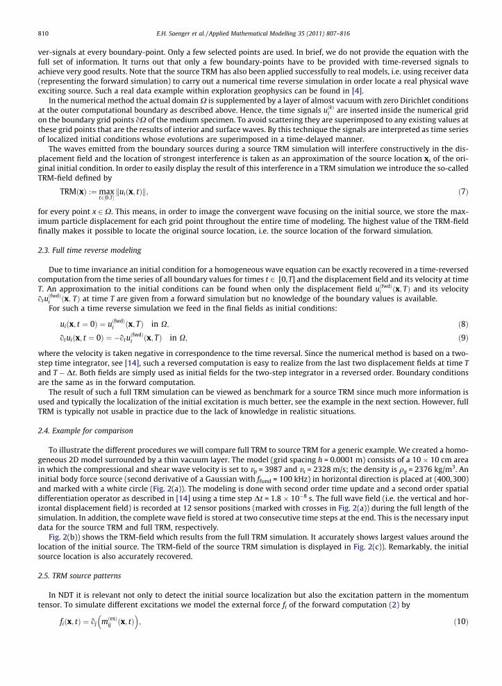
To illustrate the different procedures we will compare full TRM to source TRM for a generic example. We created a homo-geneous 2D model surrounded by a thin vacuum layer. The model (grid spacing h = 0.0001 m) consists of a 10 � 10 cm areain which the compressional and shear wave velocity is set to vp = 3987 and vs = 2328 m/s; the density is qg = 2376 kg/m3. Aninitial body force source (second derivative of a Gaussian with ffund = 100 kHz) in horizontal direction is placed at (400,300)and marked with a white circle (Fig. 2(a)). The modeling is done with second order time update and a second order spatialdifferentiation operator as described in [14] using a time step Dt = 1.8 � 10�8 s. The full wave field (i.e. the vertical and hor-izontal displacement field) is recorded at 12 sensor positions (marked with crosses in Fig. 2(a)) during the full length of thesimulation. In addition, the complete wave field is stored at two consecutive time steps at the end. This is the necessary inputdata for the source TRM and full TRM, respectively.

Fig. 2(b)) shows the TRM-field which results from the full TRM simulation. It accurately shows largest values around thelocation of the initial source. The TRM-field of the source TRM simulation is displayed in Fig. 2(c)). Remarkably, the initialsource location is also accurately recovered.

2.5. TRM source patterns

In NDT it is relevant not only to detect the initial source localization but also the excitation pattern in the momentumtensor. To simulate different excitations we model the external force fi of the forward computation (2) by

fiðx; tÞ ¼ oj mðexÞij ðx; tÞ

� �; ð10Þ

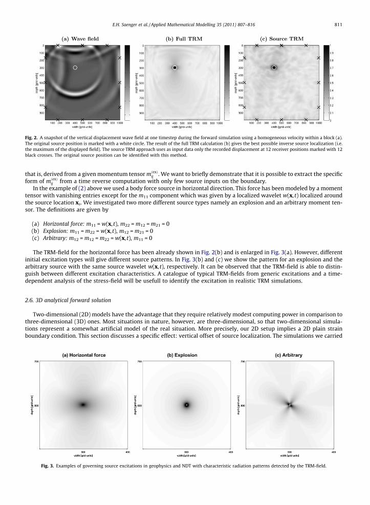
Fig. 2. A snapshot of the vertical displacement wave field at one timestep during the forward simulation using a homogeneous velocity within a block (a).The original source position is marked with a white circle. The result of the full TRM calculation (b) gives the best possible inverse source localization (i.e.the maximum of the displayed field). The source TRM approach uses as input data only the recorded displacement at 12 receiver positions marked with 12black crosses. The original source position can be identified with this method.

E.H. Saenger et al. / Applied Mathematical Modelling 35 (2011) 807–816 811

that is, derived from a given momentum tensor mðexÞij . We want to briefly demonstrate that it is possible to extract the specific

form of mðexÞij from a time reverse computation with only few source inputs on the boundary.

In the example of (2) above we used a body force source in horizontal direction. This force has been modeled by a momenttensor with vanishing entries except for the m11 component which was given by a localized wavelet w(x, t) localized aroundthe source location xs. We investigated two more different source types namely an explosion and an arbitrary moment ten-sor. The definitions are given by

(a) Horizontal force: m11 = w(x, t), m22 = m12 = m21 = 0(b) Explosion: m11 = m22 = w(x, t), m12 = m21 = 0(c) Arbitrary: m12 = m12 = m22 = w(x, t), m11 = 0

The TRM-field for the horizontal force has been already shown in Fig. 2(b) and is enlarged in Fig. 3(a). However, differentinitial excitation types will give different source patterns. In Fig. 3(b) and (c) we show the pattern for an explosion and thearbitrary source with the same source wavelet w(x, t), respectively. It can be observed that the TRM-field is able to distin-guish between different excitation characteristics. A catalogue of typical TRM-fields from generic excitations and a time-dependent analysis of the stress-field will be usefull to identify the excitation in realistic TRM simulations.

2.6. 3D analytical forward solution

Two-dimensional (2D) models have the advantage that they require relatively modest computing power in comparison tothree-dimensional (3D) ones. Most situations in nature, however, are three-dimensional, so that two-dimensional simula-tions represent a somewhat artificial model of the real situation. More precisely, our 2D setup implies a 2D plain strainboundary condition. This section discusses a specific effect: vertical offset of source localization. The simulations we carried

Fig. 3. Examples of governing source excitations in geophysics and NDT with characteristic radiation patterns detected by the TRM-field.

812 E.H. Saenger et al. / Applied Mathematical Modelling 35 (2011) 807–816

out were motivated by observations made for 2D time reverse simulations with a receiver line placed directly above theknown source and with other receiver lines positioned in a certain horizontal distance away from the first line. It was ob-served that the TRM-field of maximum particle displacement localized the source in different depths depending on the re-ceiver line chosen for the 2D time reverse simulation.

In order to understand those effects, we use a 3D analytical solution of the elastodynamic wave equation for a point forcein a homogeneous, isotropic and unbounded medium as described in Aki and Richards [13].

If a point force f in direction ej with general time-varying amplitude X0(t) acts at a particular fixed point O which wechoose to be the origin of a fixed Cartesian coordinate system and if the medium is elastic, isotropic, homogeneous and un-bounded, the displacement ui(x, t) at point x and time t in direction ei is given by the following explicit formula:

Fig. 4.right ha

ui x; tð Þ ¼ 14pq

3cicj � dij

� � 1r3

Z r=b

r=asX0 t � sð Þds

|fflfflfflfflfflfflfflfflfflfflfflfflfflfflfflfflfflfflfflfflfflfflfflfflfflfflfflfflfflfflfflfflfflfflfflfflffl{zfflfflfflfflfflfflfflfflfflfflfflfflfflfflfflfflfflfflfflfflfflfflfflfflfflfflfflfflfflfflfflfflfflfflfflfflffl}NFð Þ

þ 14pqa2 cicj

1r

X0 t � ra

� �|fflfflfflfflfflfflfflfflfflfflfflfflfflfflfflfflfflfflfflfflfflfflffl{zfflfflfflfflfflfflfflfflfflfflfflfflfflfflfflfflfflfflfflfflfflfflffl}

FFPð Þ

� 14pqb2 cicj � dij

� �1r

X0 t � rb

�|fflfflfflfflfflfflfflfflfflfflfflfflfflfflfflfflfflfflfflfflfflfflfflfflfflfflfflfflffl{zfflfflfflfflfflfflfflfflfflfflfflfflfflfflfflfflfflfflfflfflfflfflfflfflfflfflfflfflffl}

FFSð Þ

; ð11Þ

where the following notations have been used:

� r :¼ jxj denoting the distance of point x from the point, where the point force f is acting.� ci :¼ xi/r (i = 1, 2, 3) denoting cosine of direction.� a, b and q denoting P-wave, S-wave velocities and density of the medium.� dij is Kronecker’s delta.� NF stands for the near field part of the solution.� FFP stands for the far field of the compressional (P-) wave part of the solution.� FFS stands for the far field of the shear (S-) wave part of the solution.

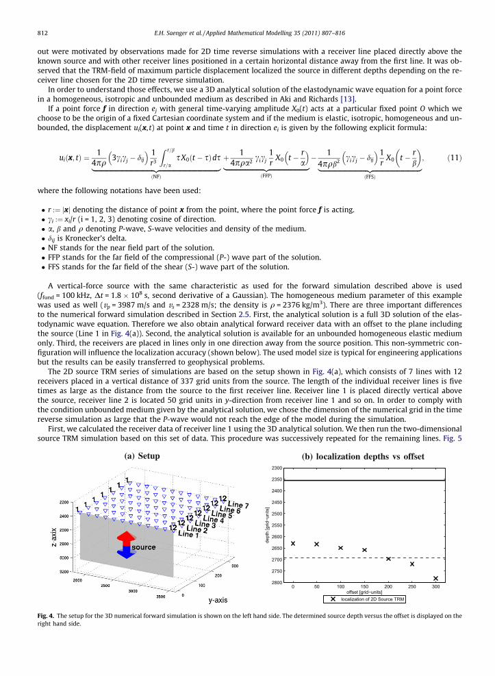
A vertical-force source with the same characteristic as used for the forward simulation described above is used(ffund = 100 kHz, Dt = 1.8 � 108 s, second derivative of a Gaussian). The homogeneous medium parameter of this examplewas used as well (vp = 3987 m/s and vs = 2328 m/s; the density is q = 2376 kg/m3). There are three important differencesto the numerical forward simulation described in Section 2.5. First, the analytical solution is a full 3D solution of the elas-todynamic wave equation. Therefore we also obtain analytical forward receiver data with an offset to the plane includingthe source (Line 1 in Fig. 4(a)). Second, the analytical solution is available for an unbounded homogeneous elastic mediumonly. Third, the receivers are placed in lines only in one direction away from the source position. This non-symmetric con-figuration will influence the localization accuracy (shown below). The used model size is typical for engineering applicationsbut the results can be easily transferred to geophysical problems.

The 2D source TRM series of simulations are based on the setup shown in Fig. 4(a), which consists of 7 lines with 12receivers placed in a vertical distance of 337 grid units from the source. The length of the individual receiver lines is fivetimes as large as the distance from the source to the first receiver line. Receiver line 1 is placed directly vertical abovethe source, receiver line 2 is located 50 grid units in y-direction from receiver line 1 and so on. In order to comply withthe condition unbounded medium given by the analytical solution, we chose the dimension of the numerical grid in the timereverse simulation as large that the P-wave would not reach the edge of the model during the simulation.

First, we calculated the receiver data of receiver line 1 using the 3D analytical solution. We then run the two-dimensionalsource TRM simulation based on this set of data. This procedure was successively repeated for the remaining lines. Fig. 5

(a) Setup (b) localization depths vs offset

0 50 100 150 200 250 300

2300

2350

2400

2450

2500

2550

2600

2650

2700

2750

2800

offset [grid−units]

dept

h [g

rid−u

nits

]

localization of 2D Source TRM

The setup for the 3D numerical forward simulation is shown on the left hand side. The determined source depth versus the offset is displayed on thend side.

Fig. 5. TRM-field for Line 1 where the receivers were located directly above the point source (grid spacing h = 0.0001 m). The time-reversed signals,determined by an analytical solution, are inserted at 12 points marked with a white circle. The cross is the maximum value of the TRM-field. There is avertical localization error with respect to the original source location (white quadrat).

E.H. Saenger et al. / Applied Mathematical Modelling 35 (2011) 807–816 813

shows the 2D-TRM-field resulting on the plane directly under the corresponding receiver line. The white square marks thelocation of the original source and the black cross the maximum value.

It is visible that the location of the maximum value shifts vertically downwards with increasing offset of the receiver linerelative to the source location (Fig. 4(b)). We display the offset of the receiver lines on the x-axis and the depth indicated bythe corresponding TRM-fields on the y-axis. We observe a clear trend to deeper depths the farther a receiver line is locatedfrom the original source. This can be explained by the non-symmetric distribution of the receivers around the source in com-bination with the non-zero wavelength of the propagating elastic waves. However, for most practical applications the ob-served localization accuracy is acceptable. More generally, we want to point out that the analytical forward solutionpresented here can also used for an analytical TRM approach in an unbounded homogeneous medium [16].

3. NDT-application: localization of acoustic emissions in concrete

3.1. Numerical concrete model

A numerical concrete model in 2D with randomly distributed concrete constituents similar to [17] is presented (Fig. 6(a)).The model displays an arbitrary cross section of the numerical concrete specimen. Plain strain is assumed for each cross sec-tion. The concrete specimen is simplified by spatial randomly distributed ellipses (grains) and circles (air voids) and filledbetween with homogeneous cement paste. The aggregates and air voids are effectively modeled as infinite cylinders. Thegrain-size distribution is transferred from a real concrete mix and is in agreement with Fuller’s curve [18]. Air inclusionsare estimated with 2%, a common limit percentage in practice. The elastic material properties for the grains (vp = 4180 m/s, vs = 2475 m/s, q = 2610 kg/m3), the air voids (vp = 0 m/s, vs = 0 m/s, q = 0.0001 kg/m3) and for the cement paste(vp = 3950 m/s, vs = 2250 m/s, q = 2050 kg/m3) are allocated to grid points for the finite-difference algorithm (grid spacingh = 0.0001 m). For reasons of verification computer tomography (CT) screens of a concrete cube (Fig. 6(b)) are provided. Com-

Fig. 6. Numerical concrete model (10 � 10 cm) versus CT screen of concrete specimen (12 � 12 cm). Displayed are normalized density values. Dark colorscorrespond to air inclusions, grey to the cement paste and ligth color defines the grains.

814 E.H. Saenger et al. / Applied Mathematical Modelling 35 (2011) 807–816

parison of properties of the introduced numerical concrete model versus the CT model (real concrete) shows a good agree-ment and suggests its effectiveness and applicability to non-destructive testing of concrete. Moreover, the numerical con-crete model can be straightforward varied with different grain size and air void distributions for further parameterstudies. However, it is also possible to use the CT screens as input for our numerical simulations. This is illustrated in thesection ’outlook’. We choose here the numerical concrete model because, (1) it can be generated with a full control of thegrain-size distribution, and (2) we want to avoid artefacts due to segmentation errors. Segmentation of raw CT data isone difficult and necessary processing step (e.g. [19] and references therein).

3.2. Forward simulation with an arbitrary chosen momentum tensor source

In order to create a synthetic but realistic data set we use the following model setup. An arbitrary chosen momentumtensor source with source time-function as described in Section 2.5 is used. The discretization details are adopted fromthe previous section. In the snapshot shown (Fig. 7(a)) a wave field excited at (400, 300) is illustrated. Due to the heteroge-neous concrete model a lot of scattering can be observed compared to the wave field in Fig. 2(a). Two-components (horizon-tal and vertical displacement) of the emitted waves are recorded at 12 sensor positions of sensors marked by black crosses onthe boundaries.

3.3. Reverse simulation with 12 sensors using exact velocity model

The time reverse computation is executed for two sensor modifications, sensors with two components (displacement nor-mal and parallel to surface) and sensors with one component (displacement normal to surface) recorded. Steiner et al. [4]applied TRM successfully on data measured with three-components seismometers. For most NDT applications (i.e. for pie-zoelectric sensors) the case where one-component data is recorded on sensor positions is relevant. The performance is ana-lyzed considering two-component sensor modification and discussed. As described before by using both components thetime-reversed propagating waves focus on the source coordinates they originated from. An excellent result is obtained(Fig. 7(b)) in that the radiation pattern of the induced source can be visual identified (marked by the white circle) by meansof the characteristic according to Fig. 3(c). Using only the displacement component normal to concrete surface a good focuscan be observed (Fig. 7(c)). The radiation pattern seems blurred, but represents a satisfying achievement if only one-compo-nent data used for reverse computation is considered.

3.4. Effective elastic properties of the used numerical concrete sample

To obtain effective velocities of the numerical concrete sample (Fig. 6(a)) we use a technique described in detail in [20]. Areview of this and related methods is given in [21]. We apply a body force plane source at the top of the model. The planewave generated in this way propagates through the numerical concrete model. With two horizontal planes of receivers at thetop and at the bottom, it is possible to measure the time-delay of the peak amplitude of the mean plane wave caused by theinhomogeneous region. With the time-delay (compared to a homogeneous reference model) one can estimate the effectivevelocity of the compressional and shear wave. The source wavelet in our experiments is always the first derivative of aGaussian with a dominant frequency of 12500 Hz and with a time increment of Dt = 1.8 � 10�8 s. As a result, we havedetermined the effective compressional wave velocity to vp,eff = 3987 m/s and the effective shear wave velocity tovs,eff = 2328 m/s.

Fig. 7. Forward simulation and reverse simulation in a heterogeneous medium for two sensor modifications.

Fig. 8. Performance of time reverse modeling using effective elastic properties for two different sensor modifications.

Fig. 9. CT screens of uncracked concrete cuboid (12 � 12 � 18 cm) with post processed numerical model for wave propagation simulation.

E.H. Saenger et al. / Applied Mathematical Modelling 35 (2011) 807–816 815

3.5. Reverse simulation with 12 sensors using effective elastic properties for concrete

Given the effective elastic properties (EEP) with vp,eff and vs,eff a reverse computation is executed similar to Section 3.3.The forward simulation is performed based on the heterogeneous medium as described in Section 3.2, but for time reversemodeling the previous determined EEPs are used instead. Considering both sensor components a very good result can beachieved (Fig. 8(a)). In the backward propagation direction no scattering will occur and compared to reverse simulation withthe exact velocity model (Fig. 7(a)) a convergence of elastic energy can be observed. The TRM source pattern is clearly visible.Using only the displacement component normal to the concrete surface a problematic result can be obtained (Fig. 8(b)). Arti-facts due to surface waves are significantly visible around the boundaries and the source pattern is displayed rudimentary.Possible solutions to improve the localization are to place more sensors on the surface and to magnify the energy inducedinto the model and to interpolate the zero values on the boundary between sensor positions with respect to the incomingwaves hitting the boundary. An irregular sensor arrangement may be investigated to improve the performance of the meth-od and to clarify their influence on the wave focus.

4. Outlook

The forthcoming approach aims at extending the introduced two-dimensional TRM method to three dimensions. Weshow the first steps of this approach.

A concrete specimen screened in thin slices (Fig. 9(a)) is considered and after post processing (e.g. threshold-segmenta-tion) visualized as a complete three-dimensional model (Fig. 9(b)). The digital format is beneficial for further considerationssuch as simulations of elastic wave propagation.

816 E.H. Saenger et al. / Applied Mathematical Modelling 35 (2011) 807–816

The segmented CT data can be read and translated into a feasible format for wave propagation computations on a FD grid.Elastic material properties such as p-wave velocity cp and S-wave velocity cs are allocated to the segmented aggregates.Numerical simulations starting a double-couple source excitation (Fig. 9(c)) are performed on the high performance parallelcomputing cluster at the central computing facilities of ETH Zurich. The influence of density distribution of aggregates, airvoids percentage and crack distribution on elastic wave propagation will be investigated separately. The numerical resultsare compared to data obtained from physical tests and are to be discussed.

The TRM method presented in this paper was transferred from exploration geophysics (km-scale) to acoustic emissionanalysis of a single concrete sample (cm-scale). Therefore we assume that this technique can also be transferred to otherNDT applications such as tubes inspection in nuclear power plants or gas-pipe inspection buried under ground. Most impor-tant is that the discussed method is able to localize a (secondary) source of acoustic waves. This can be for example a crackwhich can scatter an elastic wave in a thin plate of steel (plain strain). However, for such an application we recommend toperform numerical feasibility studies as presented in this work.

5. Conclusion

Time reverse modeling using the elastodynamic wave equation is, due to the increasing computational possibilities, now-adays fast and accurate. We used the rotated staggered FD grid to calculate effective elastic properties of concrete. Ournumerical modeling can be considered as an efficient and well-controlled computer experiment. The numerical simulationsshow that source areas and characteristics of acoustic emissions can be located using TRM. With our feasibility study wedemonstrate that our approach is ready to be applied in the laboratory for a deeper understanding of experiments in the areaof non-destructive testing. We have demonstrated that with a limited number of sensors and an effective homogeneous elas-tic model the accuracy of localization is acceptable.

Acknowledgments

The authors are grateful because the CT screens used (Figs. 6(a) and 9(a)) were kindly provided by Dr. Thomas Frauenf-elder from the Institute of Diagnostic Radiology of the University Hospital Zurich. Constructive anonymous reviewers haveimproved this work significantly. Prof. Thomas Vogel from the Institute of Structural Engineering of ETH Zurich is acknowl-edged for supporting the methods used. E.H. Saenger thanks the DFG (Deutsche Forschungsgemeinschaft) for their supportthrough the Heisenberg Programme (SA 996/1-1). M. Torrilhon is funded through an EURYI-Award of the European ScienceFoundation.

References

[1] M. Fink, Time-reversed acoustics, Sci. Am. (1999) 67–73.[2] H. Kao, S.-J. Shan, The source-scanning algorithm: mapping the distribution of seismic sources in time and space, Geophys. J. Int. (2004) 589–594.[3] D. Gajewski, E. Tessmer, Reverse modelling for seismic event characterization, Geophys. J. Int. (2005) 276–284.[4] B. Steiner, E.H. Saenger, S.M. Schmalholz, Time reverse modeling of low-frequency microtremors: a potential method for hydrocarbon reservoir

localization, Geophys. Res. Lett. 35 (2008) L03307.[5] T. Shiotani, D.G. Aggelis, Wave propagation in cementitious material containing artificial distributed damage, Mater. Struct. 42 (2009) 377–384.[6] C.U. Grosse, Advances in Construction Materials, Springer, Heidelberg, 2007, ISBN 978-3-540-72447-6.[7] P. Fellinger, R. Marklein, K.-J. Langenberg, S. Klaholz, Numerical modeling of elastic wave propagation and scattering with EFIT – elastodynamic finite

integration technique, Wave Motion 21 (1995) 47–66.[8] F. Schubert, Numerical time-domain modeling of linear and nonlinear ultrasonic wave propagation using finite integration techniques – theory and

applications, Ultrasonics 42 (2004) 221–229.[9] F. Schubert, B. Köhler, Ten lectures on impact-echo, J. Nondestruct. Eval. 27 (2008) 5–21.

[10] B. Schechinger, T. Vogel, Acoustic emission for monitoring a reinforced concrete beam subject to four-point-bending, Constr. Build. Mater. 21 (2007)483–490.

[11] C.U. Grosse, M. Ohtsu, Acoustic Emission Testing: Basics for Research – Applications in Civil Engineering; With Contributions by Numerous Experts,Springer, Heidelberg, 2008, ISBN 978-3-540-69895-1.

[12] M. Fink, Time reversal of ultrasonic fields – part 1: basic principles, IEEE Trans. Ultrason. Ferroelectr. Freq. Control 39 (5) (1992) 555–566.[13] K. Aki, P.G. Richards, Quantitative Seismology, Theory and Methods, W.H. Freeman and Company, San Fransisco, 1980.[14] E.H. Saenger, N. Gold, S.A. Shapiro, Modeling the propagation of elastic waves using a modified finite-difference grid, Wave Motion 31 (1) (2000) 77–

92.[15] E.H. Saenger, T. Bohlen, Anisotropic and viscoelastic finite-difference modeling using the rotated staggered grid, Geophysics 69 (2) (2004) 583–591.[16] B. Steiner, Time reverse modeling of low-frequency tremor sources, Dissert. ETH Zurich (2009) 1826.[17] S. Häfner, S. Eckhardt, T. Luther, C. Könke, Mesoscale modeling of concrete: geometry and numerics, Comput. Struct. 84 (2006) 450–461.[18] W.B. Fuller, S.E. Thomson, The laws of proportioning concrete, Trans. Am. Soc. Civ. Eng. 59 (1907) 67–143.[19] Y. Yao, D. Liua, Y. Chea, D. Tanga, S. Tanga, W. Huanga, Non-destructive characterization of coal samples from china using microfocus X-ray computed

tomography, Int. J. Coal Geol. 80 (2009) 113–123.[20] E.H. Saenger, S.A. Shapiro, Effective velocities in fractured media: a numerical study using the rotated staggered finite-difference grid, Geophys.

Prospect. 50 (2) (2002) 183–194.[21] E.H. Saenger, Numerical methods to determine effective elastic properties, Int. J. Eng. Sci. (2008) 598–605.