Application of Spatial Veriﬁcation Methods to … of Spatial Veriﬁcation Methods to Idealized...

Application of Spatial Verification Methods to Idealized and NWP-GriddedPrecipitation Forecasts

DAVID AHIJEVYCH, ERIC GILLELAND, AND BARBARA G. BROWN

National Center for Atmospheric Research,* Boulder, Colorado

ELIZABETH E. EBERT

Centre for Australian Weather and Climate Research, Melbourne, Victoria, Australia

(Manuscript received 27 April 2009, in final form 24 September 2009)

ABSTRACT

Several spatial forecast verification methods have been developed that are suited for high-resolution pre-

cipitation forecasts. They can account for the spatial coherence of precipitation and give credit to a forecast that

does not necessarily match the observation at any particular grid point. The methods were grouped into four

broad categories (neighborhood, scale separation, features based, and field deformation) for the Spatial

Forecast Verification Methods Intercomparison Project (ICP). Participants were asked to apply their new

methods to a set of artificial geometric and perturbed forecasts with prescribed errors, and a set of real forecasts

of convective precipitation on a 4-km grid. This paper describes the intercomparison test cases, summarizes

results from the geometric cases, and presents subjective scores and traditional scores from the real cases.

All the new methods could detect bias error, and the features-based and field deformation methods were

also able to diagnose displacement errors of precipitation features. The best approach for capturing errors in

aspect ratio was field deformation. When comparing model forecasts with real cases, the traditional verifi-

cation scores did not agree with the subjective assessment of the forecasts.

1. Introduction

With advances in computing power, numerical guid-

ance has become available on increasingly finer scales.

Mesoscale phenomena such as squall lines and hurricane

rainbands are routinely forecasted. While the simulated

reflectivity field and precipitation distribution have

more realistic spatial structure and can provide valuable

guidance to forecasters on the mode of convective

evolution (Weisman et al. 2008), the traditional verifi-

cation scores often do not reflect improvement in per-

formance over coarse-grid models. Small errors in the

position or timing of small convective features result in

false alarms and missed events that dominate traditional

categorical verification scores (Wilks 2006). This prob-

lem is exacerbated by smaller grid spacing. Several tra-

ditional scores such as critical success index (CSI; or

threat score) and Gilbert skill score (GSS; or equitable

threat score) have been used for decades to track model

performance, but their utility is limited when it comes to

diagnosing model errors such as a displaced forecast

feature or an incorrect mode of convective organization.

To meet the need for more informative forecast eval-

uation, novel spatial verification methods have been de-

veloped. An overarching effort to compare and contrast

these new methods and coordinate their development

is called the Spatial Forecast Verification Methods In-

tercomparison Project (ICP). The ICP stemmed from

a verification workshop originally held in Boulder, Col-

orado, in 2007. A literature review by Gilleland et al.

(2009a) defines four main categories of new methods:

neighborhood, scale separation, features based, and field

deformation, a convention that is also used here.

In the ICP, a common set of forecasts was evalu-

ated by participants in the project using one or more of

the new methods. In sections 2 and 3, we describe the

* The National Center for Atmospheric Research is sponsored

by the National Science Foundation.

Corresponding author address: David Ahijevych, National

Center for Atmospheric Research, P.O. Box 3000, Boulder, CO

80307-3000.

E-mail: [email protected]

DECEMBER 2009 A H I J E V Y C H E T A L . 1485

DOI: 10.1175/2009WAF2222298.1

� 2009 American Meteorological Society

geometric and perturbed datasets that were analyzed by

ICP participants. In section 4, we present nine real cases

and offer examples of traditional scores and results of an

informal subjective evaluation of the forecasts for the

nine cases. Readers are encouraged to use this paper

along with that of Gilleland et al. (2009a) to identify new

methods that may be appropriate for their needs, and

then delve into the more detailed papers on the in-

dividual methods. This set of papers makes up a special

collection of Weather and Forecasting on the Spatial

Verification Methods Intercomparison Project (Casati

2010; Brill and Mesinger 2009; Davis et al. 2009; Ebert

2009; Ebert and Gallus 2009; Gilleland et al. 2009b,

manuscript submitted to Wea. Forecasting, hereafter

GLL; Keil and Craig 2009; Lack et al. 2010; Marzban

and Sandgathe 2009; Marzban et al. 2009; Mittermaier

and Roberts 2010; Nachamkin 2009; Wernli et al. 2009).

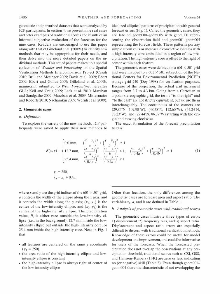
2. Geometric cases

a. Definition

To explore the variety of the new methods, ICP par-

ticipants were asked to apply their new methods to

idealized elliptical patterns of precipitation with general

forecast errors (Fig. 1). Called the geometric cases, they

are labeled geom000–geom005 with geom000 repre-

senting the observation field and geom001–geom005

representing the forecast fields. These patterns portray

simple storm cells or mesoscale convective systems with

a high-intensity core embedded in a region of low pre-

cipitation. The high-intensity core is offset to the right of

center within each feature.

The geometric cases were defined on a 601 3 501 grid

and were mapped to a 601 3 501 subsection of the Na-

tional Centers for Environmental Prediction (NCEP)

storage grid 240 (Dey 1998) for verification purposes.

Because of the projection, the actual grid increment

ranges from 3.7 to 4.3 km. Going from a Cartesian to

a polar stereographic grid, the terms ‘‘to the right’’ and

‘‘to the east’’ are not strictly equivalent, but we use them

interchangeably. The coordinates of the corners are

(29.848N, 109.988W), (48.388N, 112.608W), (44.248N,

78.238W), and (27.448N, 86.778W) starting with the ori-

gin and moving clockwise.

The exact formulation of the forecast precipitation

field is

R(x, y) 5

0.0 mm,x� x

1

a

� �2

1y� y

1

b

� �2

$ 1

12.7 mm,x� x

1

a

� �2

1y� y

1

b

� �2

, 1,x� x

2

0.4a

� �2

1y� y

1

0.4b

� �2

$ 1

25.4 mm,x� x

2

0.4a

� �2

1y� y

1

0.4b

� �2

, 1

8>>>>><>>>>>:

(1)

y1

5 250,

x2

5 x1

1 0.4a,

where x and y are the grid indices of the 601 3 501 grid,

a controls the width of the ellipse along the x axis, and

b controls the width along the y axis; (x1, y1) is the

center of the low-intensity ellipse, and (x2, y1) is the

center of the high-intensity ellipse. The precipitation

value, R, is either zero outside the low-intensity el-

lipse (i.e., in the background), 12.7 mm inside the low-

intensity ellipse but outside the high-intensity core, or

25.4 mm inside the high-intensity core. Note in Fig. 1

that

d all features are centered on the same y coordinate

(y1 5 250)d the area ratio of the high-intensity ellipse and low-

intensity ellipse is constantd the high-intensity ellipse is always right of center of

the low-intensity ellipse

Other than location, the only differences among the

geometric cases are forecast area and aspect ratio. The

variables x1, a, and b are defined in Table 1.

b. Analysis of geometric cases with traditional scores

The geometric cases illustrate three types of error:

1) displacement, 2) frequency bias, and 3) aspect ratio.

Displacement and aspect ratio errors are especially

difficult to discern with traditional verification methods.

Knowledge of these errors could be useful for model

development and improvement, and could be informative

for users of the forecasts. When the forecasted pre-

cipitation does not overlap the observations at any pre-

cipitation threshold, traditional scores such as CSI, GSS,

and Hanssen–Kuipers (H-K) are zero or less, indicating

no (or negative) skill (Table 2). Even though geom001–

geom004 share the characteristic of not overlapping the

1486 W E A T H E R A N D F O R E C A S T I N G VOLUME 24

observation, geom003 has slightly higher probability of

false detection and lower H-K, Heidke skill score (HSS),

and GSS than the others because the larger forecast

object increases the false alarm rate and decreases the

correct forecasted null events.

The first two geometric cases, geom001 and geom002,

illustrate pure displacement errors. The geom001 fore-

cast feature shares a border with the observation, but the

geom002 case is displaced much farther to the right.

The geom001 case is clearly superior to geom002, but the

traditional verification scores (column 2 of Table 2) sug-

gest they are equally poor. Moreover, the geom004 fore-

cast exhibits a very different kind of error from geom001

and 002, yet the traditional verification measures have

equivalent values for all three of these cases. In contrast,

some of the new spatial verification methods are able to

distinguish the differences in performance for these three

cases and quantify the displacement (and other) errors.

The geom003 and geom005 forecast areas are both

stretched in the x dimension, illustrating frequency bias.

FIG. 1. (a)–(f) Five simple geometric cases derived to illustrate specific forecast errors. The

forecasted feature (red) is positioned to the right of the observed feature (green). Note, in (f)

(geom005), the forecast and observation features overlap. One grid box is approximately 4 km

on a side.


Traditional bias scores do pick up the frequency bias,

and the RMSE is largest for geom005, but the behavior

of some other traditional scores is troubling. In par-

ticular, geom005 has an extremely high-frequency bias,

but its false alarm ratio, H-K, GSS, and CSI scores are

superior to all other geometric cases (Table 2). Those

scores only give credit if the forecast event overlaps the

observation. To be fair, a hydrologist might actually

prefer geom005, even if it is considered to be extremely

poor by modelers and other users. Nevertheless, a larger

CSI value does not necessarily indicate that the forecast

is better overall, which is why these traditional scores

can be misleading when used in isolation.

The final type of error in the geometric forecasts is

aspect ratio. Although the geom004 forecast resembles

a simple rotation of the observed feature, geom004 ac-

tually illustrates an error in aspect ratio. In particular,

the zonal width is 4 times too large, and the meridional

extent is too narrow.

In the following analysis of the spatial verification

methods, we address three questions pertaining to the

geometric cases:

1) Does geom001 score better than geom002 and is the

error correctly attributed to displacement?

2) Is the method sensitive to the increasing frequency

bias in geom003 and geom005?

3) Can the method diagnose the aspect ratio error in

geom004?

Table 3 summarizes the answers to these questions,

which are discussed in greater detail below. Note that

the paper of Gilleland et al. (2009a) answers a different

set of questions that addresses the nature of the infor-

mation provided by the various spatial verification

methods.

c. Neighborhood methods applied to geometric cases

The neighborhood methods (Ebert 2009; Mittermaier

and Roberts 2010) look in progressively larger space–

time neighborhoods about each grid square and compare

the sets of probabilistic, continuous, or categorical values

from the forecast to the observation. These methods are

sensitive to the greater displacement error in geom002

versus geom001, but because they are not based on

features, they do not provide direct information on the

feature displacement. Instead, the neighborhood meth-

ods show that larger neighborhoods are necessary for

geom002 to reach the same performance as geom001. For

example, Mittermaier and Roberts (2010) show that

TABLE 1. The parameters used in Eq. (1) to define the geometric

precipitation fields in Fig. 1. Displacement in the x direction is

governed by x1, a is the width of the ellipse in the x dimension, and

b is the width of the ellipse in the y dimension. These are all in

terms of grid points, or approximately 4 km. The aspect ratio of the

ellipse is the unitless ratio a/b.

Name x1 a b

Aspect ratio

a/b

(a) geom000 200 25 100 0.25

(b) geom001 250 25 100 0.25

(c) geom002 400 25 100 0.25

(d) geom003 325 100 100 1.0

(e) geom004 325 100 25 4.0

(f) geom005 325 200 100 2.0

TABLE 2. Traditional verification scores applied to geometric

cases where R . 0. These statistics were calculated with the

grid_stat tool, part of the MET verification package (NCAR 2009).

Traditional score geom001/002/004 geom003 geom005

Accuracy 0.95 0.87 0.81

Frequency bias 1.00 4.02 8.03

Multiplicative

intensity bias

1.00 4.02 8.04

RMSE (mm) 3.5 5.6 6.9

Bias-corrected

RMSE (mm)

3.5 5.5 6.3

Correlation

coefficient

20.02 20.05 0.20

Probability of

detection

0.00 0.00 0.88

Probability of false

detection

0.03 0.11 0.19

False alarm ratio 1.00 1.00 0.89

Hanssen–Kuipers

discriminant (H-K)

20.03 20.11 0.69

Threat score or CSI 0.00 0.00 0.11

Equitable threat

score or GSS

20.01 20.02 0.08

HSS 20.03 20.04 0.16

TABLE 3. This table indicates whether each category of verification method tested in the ICP diagnosed the types of error illustrated in the

geometric cases.

Method category

Error type (geometric case) Neighborhood Scale separation Features based Field deformation

Displacement (geom001 geom002) No No Yes Yes

Frequency bias (geom003 geom005) Yes Yes Yes Yes

Aspect ratio–‘‘quasi-rotation’’ (geom004) No No No Yes


geom001 exhibits Fractions skill score (FSS) above zero

with neighborhoods larger than 200 km, but geom002 has

no skill with any reasonably sized neighborhood. Aptly,

according to FSS, the skillful neighborhood size for

geom001 (200 km) corresponds exactly to the prescribed

displacement error of 200 km.

The neighborhood methods do detect the frequency

bias of forecast geom003 and geom005, but the grossly

overforecasted geom005 has better skill scores at small

scales because it overlaps the observations. This holds

true for FSS (Mittermaier and Roberts 2010), condi-

tional bias difference (Nachamkin 2009), the multievent

contingency table (Atger 2001; Ebert 2009), and prac-

tically perfect hindcast (Brooks et al. 1998; Ebert 2009).

As the size of the neighborhood approaches the grid

scale, the neighborhood method scores match the scores

from traditional methods.

The neighborhood methods do not explicitly measure

displacement or structure error, so the aspect ratio error

in geom004 is difficult to diagnose.

d. Scale separation applied to geometric cases

The intensity-scale separation (IS) method of Casati

(2010) and the variogram approach of Marzban and

Sandgathe (2009) and Marzban et al. (2009) are sensitive

to the displacement errors in geom001 and geom002, but

they do not quantify them. The IS method (Casati 2010)

uses wavelets to decompose the difference field between

the observed binary field and the forecast binary field.

For geom001, there is a sharp minimum in the IS skill

score at the spatial scale of 128 km and a rapid rebound

to IS . 0 for scales of 512 and 1024 km (Fig. 7a of Casati

2010; 12.7-mm threshold). For geom002, the IS skill

scores are much lower at scales of 512 and 1024 km

relative to geom001 (Fig. 7b of Casati 2010). The vario-

gram approach compares the texture of the forecasted

field to the observations at different spatial scales.

Similar to the IS method, the variogram of Marzban and

Sandgathe (2009) and Marzban et al. (2009) is sensitive

to displacement error, but does not isolate the magni-

tude of the displacement.

The frequency bias of geom003 and geom005 results in

a large drop in IS skill score at the largest spatial scales

(2048 km; Casati 2010). Variograms also have the poten-

tial to detect the frequency bias in geom003 and geom005,

but only if zero pixels are included (Marzban et al. 2009).

As with the neighborhood methods, neither of these

scale-separation methods is designed to detect the aspect-

ratio error in geom004.

e. Features-based methods applied to geometric cases

Features-based methods (Gilleland et al. 2009a) di-

vide a gridded field into objects by grouping clusters of

similar points. For the geometric cases, the low-intensity

or high-intensity ellipses could represent the objects. If

the forecast object is matched to the observed object,

attributes such as position and size can be compared. If

they are too distant, no match occurs and no diagnostic

information about displacement or area bias is derived.

Several features-based methods were able to quantify

the displacement errors in geom001 and geom002. The

structure, amplitude, and location (SAL) quality measure

(Wernli et al. 2008) does not provide an actual distance,

but it provides a normalized location error (L) with

higher values associated with more displacement error.

For geom001, L 5 0.11, and for geom002, L 5 0.39

(Wernli et al. 2009). The Method for Object-Based

FIG. 2. (top) The forecast and observation field for the geom004

case (adapted from GLL). (bottom) The image warping technique

(GLL) attempts to morph the forecast to the observation, and the

resultant displacement vectors are shown (along with the original

forecast field). The aspect ratio error is clearly diagnosed by the

deformation in the displacement vector field.


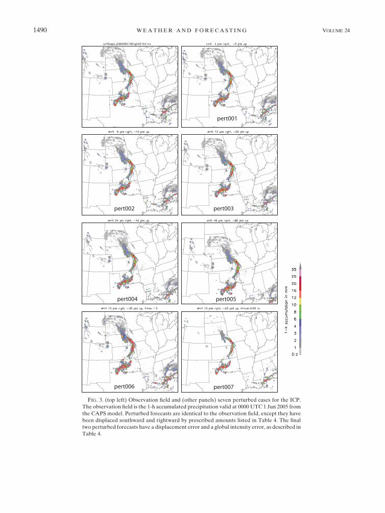
FIG. 3. (top left) Observation field and (other panels) seven perturbed cases for the ICP.

The observation field is the 1-h accumulated precipitation valid at 0000 UTC 1 Jun 2005 from

the CAPS model. Perturbed forecasts are identical to the observation field, except they have

been displaced southward and rightward by prescribed amounts listed in Table 4. The final

two perturbed forecasts have a displacement error and a global intensity error, as described in

Table 4.


Diagnostic Evaluation (MODE; Davis et al. 2009) quan-

tifies the displacement error perfectly because it matches

the forecasted and observed precipitation features and

uses centroid distance as one of the matching criteria.

The Procrustes object-oriented verification scheme also

matches objects based on their centroid distance. Lack

et al. (2010) show that the Procrustes method measures

the right amount of displacement (200 and 800 km) in

geom001 and geom002, as was also the case for the con-

tiguous rain area (CRA) method (Ebert and Gallus 2009).

Most of the features-based methods diagnose the

frequency bias of geom003 and geom005. In the SAL

approach (Wernli et al. 2009), the structure (S) and

amplitude (A) terms indicated the forecast objects are

too large (S 5 1.19 for geom003 and S 5 1.55 for

geom005, with S 5 0 being perfect) and the domain-

average precipitation amounts are too high (A 5 1.19 for

geom003 and A 5 1.55 for geom005, with 0 being per-

fect). The contiguous rain area (Ebert and Gallus 2009),

MODE (Davis et al. 2009), and Procrustes methods

(Lack et al. 2010) are also sensitive to the frequency bias

with a greater proportion of error attributed to fre-

quency bias in geom005 than in geom003.

The features-based methods diagnose the aspect ratio

error of geom004 as an orientation angle error [MODE

(Davis et al. 2009); Procrustes (Lack et al. 2010)] or ge-

neric ‘‘pattern’’ error (Ebert and Gallus 2009), or they are

insensitive to this type of error (SAL; Wernli et al. 2009).

f. Field deformation methods applied togeometric cases

Field deformation methods attempt to morph the

forecast and/or observation fields to look like each

other, minimizing a score such as RMSE. As long as the

search radius exceeds the displacement error, the dis-

placement errors of geom001 and geom002 can be quan-

tified. Keil and Craig (2009) use a pyramidal matching

algorithm to derive displacement vector fields and com-

pute a score based on displacement and amplitude (DAS).

For geom001 the displacement component dominates

the DAS as expected, but for geom002 the amplitude

component dominates the DAS because the features are

farther apart than the search radius. Optical flow tech-

niques behave similarly. A small displacement error

such as in geom001 has a trivial optical flow field that

simply shifts the object from one location to another.

However, when the forecast object is beyond the optical

flow search radius, the optical flow vectors converge on

the forecast object and attempt to ‘‘shrink’’ the apparent

false alarm (C. Marzban 2009, personal communica-

tion). The Forecast Quality Index (FQI; Venugopal

et al. 2005) utilizes the partial Hausdorff distance (PHD)

to characterize the global distance between binary im-

ages. The PHDs for geom001 and geom002 are 41 and

191 grid points, respectively, which are slightly less than

the actual displacements (50 and 200 grid points).

The field deformation methods are sensitive to fre-

quency bias. Since the forecast objects in geom003 and

geom005 are too big, the field deformation methods

shrink the forecasted precipitation area (e.g., GLL). The

frequency biases of geom003 and geom005 may not af-

fect the amplitude component of the FQI (Venugopal

et al. 2005), but they do affect the PHD. Using the formu-

lation in Venugopal et al. (2005), the PHDs of geom003,

geom004, and geom005 were 145, 141, and 186 grid

points, respectively. This accounts for the 125 gridpoint

shift to the right and the stretching in the x dimension.

The field deformation method is the only one to truly

capture the aspect ratio error in geom004. Figure 2 il-

lustrates the image warping technique of GLL. As seen

in Fig. 2, the field deformation vectors change the aspect

ratio and do not rotate the object.

3. Perturbed cases

In addition to the geometric shapes, some ICP partici-

pants evaluated a set of perturbed precipitation forecasts

from a high-resolution numerical weather prediction

model. The verification field was actually a 24-h forecast of

1-h accumulated precipitation provided by the Center for

Analysis and Prediction of Storms (CAPS) valid at 0000

UTC 1 June 2005 (Fig. 3). Perturbed forecasts were made

by shifting the entire field to the right and southward by

different amounts (Table 4). The fields were provided on

TABLE 4. Perturbed cases and their known errors. Some ICP authors use the prefix fake, instead of pert.

Perturbed case name Applied error

Pert000 No error/observation

Pert001 3 points right, 5 points down (;12 km east, ;15 km south)





Pert006 12 points right, 20 points down (;48 km east, ;80 km south), 31.5

Pert007 12 points right, 20 points down (;48 km east, ;80 km south), 21.27 mm


FIG. 4. One-hour accumulated precipitation and three corresponding model forecasts for nine real cases. The observations and forecasts

are valid at 0000 UTC on the date indicated. The upper left quadrant is the stage II observation, and quadrants A–C contain the 24-h

forecasts from the wrf2caps, wrf4ncar, and wrf4ncep models, respectively. For the subjective evaluation, the model forecasts were not

labeled and were randomly ordered.


the same 4-km grid used in the geometric cases. Additional

details about the model are provided in Kain et al. (2008).

Pixels that shifted out of the domain were discarded and

pixels that shifted into the domain were set to zero. In the

last two perturbed cases, the displacement error was held

constant, but the precipitation field in pert006 was multi-

plied by 1.5 and the field in pert007 had 1.27 mm sub-

tracted from it. Values less than zero were set to zero in

pert007. This paper does not describe the verification re-

sults for the perturbed cases, but interested readers can

consult the papers describing the individual spatial verifi-

cation methods for more detailed discussion of these cases.

4. Real cases

a. Model description

For the real precipitation examples, we use nine cases

from the 2005 Spring Program. These cases were pre-

sented to a panel of 26 scientists attending a workshop

on spatial verification methods to obtain their subjective

assessments of forecast performance (Fig. 4). The three

forecast models were run for the 2005 Spring Program

sponsored by the Storm Prediction Center (SPC) and

the National Severe Storms Laboratory (NSSL) (http://

www.nssl.noaa.gov/projects/hwt/sp2005.html). Two of

the three numerical models [provided by the National

Center for Atmospheric Research (NCAR) and NCEP

Environmental Modeling Center (EMC)] were run on

a 4-km grid, while one (CAPS) was run on a 2-km grid

and mapped to a 4-km grid. The models are denoted

wrf4ncar, wrf4ncep, and wrf2caps, respectively. Addi-

tional information on the model configurations can be

found in Kain et al. (2008). All forecasts and observations

were remapped onto the same (;4 km) grid used for the

geometric cases. This remapping method maintains, to

a desired accuracy, the total precipitation on the original

FIG. 4. (Continued)


grid and is part of the NCEP iplib interpolation library

that is routinely used and distributed by NCEP as part

of the Weather Research and Forecasting (WRF) post-

processing system. This interpolation performs a nearest-

neighbor interpolation from the original grid to a 5 3 5

set of subgrid boxes on the output grid centered on each

output grid point. A simple average of the 5 3 5 subgrid

boxes results in the interpolated value (M. Baldwin 2009,

personal communication).

The panel compared the three aforementioned models

to the stage II precipitation analysis (Lin and Mitchell

2005) for a lead time of 24 h and an accumulation interval

of one hour. Panelists rated the models’ performance

on a scale from 1 to 5, ranging from poor to excellent.

For fairness, the models were ordered randomly and not

labeled.

b. Traditional scores and subjective evaluation

The panel’s subjective scores are alternative view-

points, not definitive assessments of forecast perfor-

mance. The evaluators were not asked to consider the

usefulness of the forecasts from the standpoint of any

particular user (e.g., water manager, farmer, SPC fore-

caster) or to focus on a particular region, but to sub-

jectively evaluate the forecast as a whole. Afterward,

several of the panel members indicated that more

guidance was needed in these areas, because the use-

fulness of a forecast depends greatly on the perceived

needs of the user and the geographical area of concern;

sometimes a model performed well in one region and

poorly in another. But in order to keep the study simple,

participants were asked to simply give an overall im-

pression of the models’ skill and were left to themselves

to decide what mattered most.

Although the evaluation was performed twice in order

to increase the stability of the overall responses and to

assess the natural variability from one trial to the next,

several aspects of the survey added uncertainty to the

results. First, the panel members had varying professional

backgrounds, including meteorologists, statisticians, and

software engineers. Meteorologists were more likely to

consider realistic depictions of mesoscale structure (such

as in the stratiform precipitation area of a mesoscale

convective system) as an important criterion defining

a ‘‘good’’ forecast, and may have focused on different

features than scientists with a pure mathematical back-

ground. Examples of a good forecast were not provided.

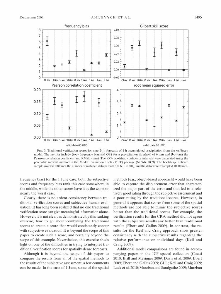
As expected with convective precipitation forecasts

on a fine grid, the traditional scores are quite poor. In

Fig. 5 we focus on the wrf4ncep model just to illustrate

this point. The scores do depend on our choice of 6 mm

as an intensity threshold. Higher thresholds correspond

to intense precipitation cores, which typically result in

even lower scores. Grid-scale prediction of convective

precipitation is not yet feasible 24 h in advance and the

GSS , 0.1 reflects that difficulty. Ideally, the frequency

bias (top left panel) would be 1, but the model consis-

tently overforecasts precipitation above 6 mm.

The slightly negative GSS for 1 and 4 June suggests

that these two forecasts are uniformly poor, however

their subjective scores tell a different story (Fig. 6). Out

of the 24 participants, 18 gave a higher score to the

1 June forecast from wrf4ncep, 4 scored them equally,

and only 2 scored 4 June higher. The panel members

were not asked to explain why they rated the 1 June

wrf4ncep forecast better than the 4 June forecast, but

there are some positive aspects of the 1 June forecast

that could play a role. Although slightly displaced, the

1 June forecast captured the overall shape of the long

band of convective precipitation curling from North

Dakota to Texas (Fig. 4). The forecasted heavy pre-

cipitation cores in the Texas Panhandle were also close

to the observed precipitation cores. On the other hand,

for 4 June, there is a prominent false alarm in the strong

north–south band of forecasted precipitation in Mis-

souri and Arkansas.

To have some objective comparison of the subjective

scores with the traditional verification scores, the sub-

jective and traditional scores are ranked in order of best

score (where one is best and nine is worst), based on

their point estimates (not including uncertainty in-

formation) for each day for the wrf4ncep model. Such

a day-to-day comparison does not account for differing

climatologies, so this is not standard practice for evalu-

ating a forecast model’s performance, but it does pro-

vide information about how traditional scores agree (or

disagree) with subjective assessments on a case-by-case

basis. The resulting ranks are displayed in Fig. 7.

It can be seen from Fig. 7 that in many cases the sub-

jective evaluations agree remarkably well with the RMSE,

but tend to disagree with the other scores. The 19 May

wrf4ncep case stands out in that there is good agreement

between the subjective scores and the frequency bias

and GSS; however, with such a high bias, the GSS is not

very interpretable for this case (indeed, only the 25 May

case is nearly unbiased). Another case that stands out

is that of 3 June where all of the scores are in good

agreement about the rank. For this day, the model

scored reasonably well for all of the summary scores, but

had a few better scores for each type of statistic on a few

other days; these other days differed depending on the

type of statistic. Similarly, the 4 June case has good

agreement for all methods that this case is regarded as

one of the worst days among these cases for this forecast

model. Finally, the subjective scores differed strongly

regarding rank from all of the other scores (except


frequency bias) for the 1 June case; both the subjective

scores and frequency bias rank this case somewhere in

the middle, while the other scores have it as the worst or

nearly the worst case.

Clearly, there is no ardent consistency between tra-

ditional verification scores and subjective human eval-

uation. It has long been realized that no one traditional

verification score can give meaningful information alone.

However, it is not clear, as demonstrated by this ranking

exercise, how to go about combining the traditional

scores to create a score that would consistently concur

with subjective evaluation. It is beyond the scope of this

paper to create such a score, and certainly beyond the

scope of this example. Nevertheless, this exercise sheds

light on one of the difficulties in trying to interpret tra-

ditional verification scores for spatially dense forecasts.

Although it is beyond the scope of this paper to

compare the results from all of the spatial methods to

the results of the subjective assessment, a few comments

can be made. In the case of 1 June, some of the spatial

methods (e.g., object-based approach) would have been

able to capture the displacement error that character-

ized the major part of the error and that led to a rela-

tively good rating through the subjective assessment and

a poor rating by the traditional scores. However, in

general it appears that scores from some of the spatial

methods are not able to mimic the subjective scores

better than the traditional scores. For example, the

verification results for the CRA method did not agree

with the subjective results any better than traditional

results (Ebert and Gallus 2009). In contrast, the re-

sults for the Keil and Craig approach show greater

consistency with the subjective results regarding the

relative performance on individual days (Keil and

Craig 2009).

Additional model comparisons are found in accom-

panying papers in the ICP special collection (Casati

2010; Brill and Mesinger 2009; Davis et al. 2009; Ebert

2009; Ebert and Gallus 2009; GLL; Keil and Craig 2009;

Lack et al. 2010; Marzban and Sandgathe 2009; Marzban

FIG. 5. Traditional verification scores for nine 24-h forecasts of 1-h accumulated precipitation from the wrf4ncep

model. The metrics include (top) frequency bias and GSS for a precipitation threshold of 6 mm and (bottom) the

Pearson correlation coefficient and RMSE (mm). The 95% bootstrap confidence intervals were calculated using the

percentile interval method in the Model Evaluation Tools (MET) package (NCAR 2009). The bootstrap replicate

sample size was 0.8 times the number of matched data pairs (0.8 3 601 3 501), and the data were resampled 1000 times.


et al. 2009; Mittermaier and Roberts 2010; Nachamkin

2009; Wernli et al. 2009). Lack et al. (2010) specifically

apply the Procrustes approach to consider the reason-

ing that may have been associated with the subjective

evaluations.

5. Summary

We constructed simple precipitation forecasts to

which traditional verification scores and some of the

recently developed spatial verification methods were

applied. These simple geometric cases illustrated poten-

tial problems with traditional scoring metrics. Displace-

ment error was easily diagnosed by the features-based

and field deformation methods, but the signal was not as

clear cut in the neighborhood and scale separation

methods, sometimes getting mixed with frequency bias

error. Errors in aspect ratio affected some of the scores

for neighborhood and scale separation approaches, but

the aspect ratio error itself was diagnosed by only a

couple of specialized configurations of the features

methods. Typically, the features-based methods treat

aspect ratio error as rotation and/or displacement. The

field deformation methods seemed to have the best

ability to directly measure errors in aspect ratio.

For the more realistic cases that we tested, each

method provided different aspects of forecast quality.

Compared to the subjective scores, the traditional ap-

proaches were particularly insensitive to changes in per-

ceived forecast quality at high-precipitation thresholds

($6 mm h21). In these cases, the newer features-based,

scale-separation, neighborhood, and field deformation

methods have the ability to give credit for close fore-

casts of precipitation features or resemblance of overall

texture to the observations.

It should be pointed out that the four general cate-

gories into which we have classified the various methods

are only used to give a general idea of how a method

describes forecast performance. Some methods fall only

loosely into a specific category (e.g., cluster analysis,

variograms, FQI). Further, it is conceivable to combine

the categories to provide even more robust measures of

forecast quality. This has been done, for example, in

Lack et al. (2010), who apply a scale separation method as

part of a features-based approach. Results shown here

should not only assist a user in choosing which methods to

use, but might also point out potentially useful combi-

nations of approaches to method developers and users.

Upon examining the results from the subjective eval-

uation, it became clear that a more rigorous experiment

with more controlled parameters would be preferred. A

more robust evaluation with a panel of experts would

undoubtedly require pinning down the region of in-

terest, isolating the potential users’ needs, and providing

a concrete definition of a good forecast. This type of

exercise, which would be best done in collaboration with

social scientists and survey experts, is left for future

work.

Acknowledgments. Thanks to Mike Baldwin who

supplied the Spring 2005 NSSL/SPC cases for the sub-

jective evaluation. Thanks to Christian Keil, Jason

Nachamkin, Bill Gallus, and Caren Marzban for their

helpful comments and additions. Also thanks to Heini

Wernli and the other two anonymous reviewers who

FIG. 6. Mean subjective scores for three models. Participants

rated the nine cases on a scale from 1 to 5 with 1 being poor and 5

being excellent. These scores are based on the two-trial mean from

24 people. The capped vertical bars are 61.96 standard error, or the

95% confidence interval, assuming the sample mean is normally

distributed.FIG. 7. Subjective ranking (x axis) vs traditional score ranking

(y axis) for the wrf4ncep model. If the traditional score were cor-

related well with the subjective ranking, one would expect the

points to fall along a line with a slope of one. The other two models

(not shown) share the same overall lack of correspondence be-

tween the traditional score rankings and the subjective ranking.


helped guide this work to completion. Randy Bullock

and John Halley-Gotway wrote the MET statistical

software package and helped with its implementation.

This work was supported by NCAR.

REFERENCES

Atger, F., 2001: Verification of intense precipitation forecasts from

single models and ensemble prediction systems. Nonlinear

Processes Geophys., 8, 401–417.

Brill, K. F., and F. Mesinger, 2009: Applying a general analytic

method for assessing bias sensitivity to bias-adjusted threat

and equitable threat scores. Wea. Forecasting, 24, 1748–1754.

Brooks, H. E., M. Kay, and J. A. Hart, 1998: Objective limits

on forecasting skill of rare events. Preprints, 19th Conf. on

Severe Local Storms, Minneapolis, MN, Amer. Meteor. Soc.,

552–555.

Casati, B., 2010: New developments of the intensity-scale technique

within the Spatial Verification Methods Inter-Comparison

Project. Wea. Forecasting, in press.

Davis, C. A., B. G. Brown, R. Bullock, and J. Halley-Gotway, 2009:

The method for object-based diagnostic evaluation (MODE)

applied to numerical forecasts from the 2005 NSSL/SPC

Spring Program. Wea. Forecasting, 24, 1252–1267.

Dey, C. H., cited 1998: Grid identification (PDS Octet 7): Master

list of NCEP storage grids. U.S. Department of Commerce

Office Note 388, GRIB ed. 1 (FM92), NOAA/NWS. [Avail-

able online at http://www.nco.ncep.noaa.gov/pmb/docs/on388/

tableb.html#GRID240.]

Ebert, E. E., 2009: Neighborhood verification: A strategy for re-

warding close forecasts. Wea. Forecasting, 24, 1498–1510.

——, and W. A. Gallus, 2009: Toward better understanding of the

contiguous rain area (CRA) method for spatial forecast veri-

fication. Wea. Forecasting, 24, 1401–1415.

Gilleland, E., D. Ahijevych, B. G. Brown, B. Casati, and E. E. Ebert,

2009a: Intercomparison of spatial forecast verification methods.

Wea. Forecasting, 24, 1416–1430.

Kain, J. S., and Coauthors, 2008: Some practical considerations

regarding horizontal resolution in the first generation of op-

erational convection-allowing NWP. Wea. Forecasting, 23,

931–952.

Keil, C., and G. C. Craig, 2009: A displacement and amplitude

score employing an optical flow technique. Wea. Forecasting,

24, 1297–1308.

Lack, S. A., G. L. Limpert, and N. I. Fox, 2010: An object-oriented

multiscale verification scheme. Wea. Forecasting, in press.

Lin, Y., and K. E. Mitchell, 2005: The NCEP Stage II/IV hourly

precipitation analyses: Development and applications. Pre-

prints, 19th Conf. on Hydrology, San Diego, CA, Amer. Me-

teor. Soc., 1.2. [Available online at http://ams.confex.com/ams/

pdfpapers/83847pdf.]

Marzban, C., and S. Sandgathe, 2009: Verification with variograms.

Wea. Forecasting, 24, 1102–1120.

——, ——, H. Lyons, and N. Lederer, 2009: Three spatial verifi-

cation techniques: Cluster analysis, variogram, and optical

flow. Wea. Forecasting, 24, 1457–1471.

Mittermaier, M. P., and N. Roberts, 2010: Intercomparison of spatial

forecast verification methods: Identifying skillful spatial scales

using the fractions skill score. Wea. Forecasting, in press.

Nachamkin, J. E., 2009: Application of the composite method to

the spatial forecast verification methods intercomparison

dataset. Wea. Forecasting, 24, 1390–1400.

NCAR, cited 2009: Model Evalution Tools (MET) users page.

[Available online at http://www.dtcenter.org/met/users.]

Venugopal, V., S. Basu, and E. Foufoula-Georgiou, 2005: A new

metric for comparing precipitation patterns with an applica-

tion to ensemble forecasts. J. Geophys. Res., 110, D08111,

doi:10.1029/2004JD005395.

Weisman, M. L., C. Davis, W. Wang, K. W. Manning, and

J. B. Klemp, 2008: Experiences with 0–36-h explicit convective

forecasts with the WRF-ARW model. Wea. Forecasting, 23,

407–437.

Wernli, H., M. Paulat, M. Hagen, and C. Frei, 2008: SAL—A novel

quality measure for the verification of quantitative pre-

cipitation forecasts. Mon. Wea. Rev., 136, 4470–4487.

——, C. Hofmann, and M. Zimmer, 2009: Spatial forecast verifi-

cation methods intercomparison project: Application of the

SAL technique. Wea. Forecasting, 24, 1472–1484.

Wilks, D. S., 2006: Statistical Methods in the Atmospheric Sciences.

2nd ed. Elsevier, 627 pp.


Application of Spatial Veriﬁcation Methods to … of Spatial Veriﬁcation Methods to Idealized...

Documents

Transcript of Application of Spatial Veriﬁcation Methods to … of Spatial Veriﬁcation Methods to Idealized...