THESIS FOR THE DEGREE OF LICENTIATE OF ENGINEERING

In

Solid and Structural Mechanics

Application of cohesive modeling in joining technology

Thick adhesive layers and rivet joints

SAEED SALIMI

Department of Applied Mechanics CHALMERS UNIVERSITY OF TECHNOLOGY

Gothenburg, Sweden, 2012

Application of cohesive modeling in joining technology Thick adhesive layers and rivet joints SAEED SALIMI

© SAEED SALIMI, 2012

THESIS FOR LICENTIATE OF ENGINEERING no 2012:21 ISSN 1652-8565

Department of Applied Mechanics Chalmers University of Technology SE-421 96 Gothenburg Sweden Telephone: +46(0)31-772 1000

Chalmers Reproservice Gothenburg, Sweden 2012

i

Application of cohesive modeling in joining technology Thesis for the degree of Licentiate of Engineering SAEED SALIMI Department of Applied Mechanics Chalmers University of Technology

ABSTRACT

This thesis summarizes the development of cohesive modeling of joints. It presents some

new developments regarding the effects of non-zero thickness of adhesive layers and a

novel approach of using the concept of cohesive modeling to characterize the failure

behavior of rivet joints.

The failure behavior of a thick adhesive layer loaded in mode I (peel), mode II (shear)

and mixed-mode are studied. Analytical relations are derived for the energy release rate

of DCBa-, ENFb- and MCBc-tests for pure peel, shear and mixed modes of loading,

respectively. Consequently, cohesive laws are derived from the energy release rate. The

results are used to predict the failure of three sets of TRBd-tests with similar and

dissimilar adherents bonded with a thick layer of adhesive and loaded in mixed mode.

Moreover, a model to characterize the failure behavior of rivet joints is investigated and

presented.

Data from DCB-, ENF- and MCB-experiments are evaluated and used to simulate and

predict the failure behavior of TRB-tests. The results of simulations are verified by the

results of three sets of TRB-experiments. To this end, sixteen TRB-experiments are

carried out in this work.

The main achievement of this thesis is validating the use of cohesive modeling to model

adhesively bonded joints with dissimilar adherents bonded with a thick layer of adhesive.

The proposed model for studying the failure behavior of rivet joints is also found to show

good agreement with numerical analyses.

Keywords: Thick adhesive layer, J-integral, mixed-mode cohesive failure, rivet joints,

mixed material

a Double Cantilever Beam b End Notch Flexure c Mixed-mode Cantilever Beam d Tensile Reinforced Bending

ii

iii

Preface

The work presented in this thesis has been carried out at the Mechanics of Materials research group at the University of Skövde. It is a part of a co-operation with the Mechanics of Materials group at the Department of Applied Mechanics at Chalmers University of Technology, Sweden.

First, I would like to give special thank and my deepest gratitude to my supervisor Professor Ulf Stigh, who gave me the opportunity not only to expand my knowledge in our research field but also to start a new life. I would also like to express my sincere gratitude to my assistant supervisor Dr. Svante Alfredsson for his constructive and extensive guidance and to my examiner Professor Lennart Josefson for his supports during my study. Furthermore, I would like to thank Dr. Anders Biel for his supports in performing the experiments.

Last but not least, I would like to thank my dear parents in Iran for their supports and inspiration.

Skövde, November 2012 Saeed Salimi

iv

v

Table of Contents

Abstract i Preface iii Table of Contents v 1 Introduction 1

1.1 Background 1 1.2 Objectives 3 1.3 Outlines of thesis 3

2 Theory 4 2.1 Fracture mechanics approach 4

2.1.1 Background 4 2.1.2 Failure of adhesive joints 9 2.1.3 Direct method 12 2.1.4 Derivation of J-integral for thick adhesive layers 15

2.2 Rivet joints 25 2.2.1 Introduction 25 2.2.2 Specimen design 27 2.2.3 Finite element analysis 28

2.3 Cohesive zone modeling 33 2.3.1 Introduction 33 2.3.2 Cohesive laws 34 2.3.3 Bilinear cohesive law 34

3 Experiments 44 3.1 DCB-experiment 45 3.2 ENF-experiment 49 3.3 MCB-experiment 55 3.4 TRB-experiment 60

4 Simulation of Experiments 70 4.1 ENF-simulation 71 4.2 MCB-simulation 75 4.3 TRB-simulation 80

5 Summary and Conclusions 83

References 85 Appendix: DCB-, ENF-, MCB- and TRB-tests’ data 89

Nomenclature 96

vi

1

1 Introduction

1-1 Background

Joining techniques such as bolting, riveting, welding and other conventional methods are

used by industry all over the world. An alternative method of joining has also emerged to

be highly successful: adhesive bonding. Adhesive bonding is a material joining process in

which an adhesive layer is placed between the adherents’ surfaces and solidifies to

produce an adhesive bond. Adhesively bonded joints are an alternative to mechanical

joints in engineering applications, particularly in dissimilar material joining, and provide

many advantages over conventional mechanical fasteners. Among these advantages are

lowering the fabrication cost and improving the damage tolerance, cf. Brockmann et al.

(2009). Adhesive joining provides a more uniform stress distribution along the bonded

area which enables a higher stiffness and more uniform load transmission, cf. Kinloch

(1987). Nevertheless, adhesive joints inevitably contain flaws, voids and discontinuities

within the adhesive layer and at the interfaces. Moreover, stress singularity due to elastic

mismatches which develops at the region of interface corner may initiate failure. As such,

adhesive joints sometimes fail unexpectedly and severely under a relatively low

mechanical or thermal load in service, cf. Afendi and Teramoto (2009). In order to have

high reliability and significant strength performance of adhesive joints, the strength and

fracture toughness of adhesive joints should be properly characterized and determined.

Fracture studies are usually carried out under several idealized conditions, as in the case

of linear elastic fracture mechanics. In such case, the details of the local crack tip fields

are characterized by a single macroscopic parameter such as the stress intensity factors

(KI, KII, KIII) or the corresponding energy release rates (GI, GII, GIII). These global

parameters are related to the corresponding material parameters; typically the fracture

energies, Ic IIc IIIc, ,G G G or the fracture toughnesses Ic IIc IIIc, ,K K K which determine the

critical conditions of initiation of crack growth, cf. Broek (1982). When the crack tip

experiences severe plastic yielding, the above concepts, based purely on the theory of

elasticity, are not valid and have led to the introduction of a path independent J-integral,

cf. Rice (1968). On the other hand, the fracture mechanics analysis presupposes the

existence of an infinitely sharp crack tip leading to singular crack tip fields. However, in

real materials neither the sharpness of the crack nor the stress levels near the crack tip

region can be infinite.

2

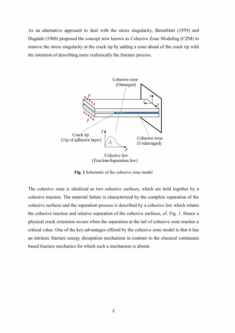
As an alternative approach to deal with the stress singularity, Barenblatt (1959) and

Dugdale (1960) proposed the concept now known as Cohesive Zone Modeling (CZM) to

remove the stress singularity at the crack tip by adding a zone ahead of the crack tip with

the intention of describing more realistically the fracture process.

Fig. 1 Schematic of the cohesive zone model

The cohesive zone is idealized as two cohesive surfaces, which are held together by a

cohesive traction. The material failure is characterized by the complete separation of the

cohesive surfaces and the separation process is described by a cohesive law which relates

the cohesive traction and relative separation of the cohesive surfaces, cf. Fig. 1. Hence a

physical crack extension occurs when the separation at the tail of cohesive zone reaches a

critical value. One of the key advantages offered by the cohesive zone model is that it has

an intrinsic fracture energy dissipation mechanism in contrast to the classical continuum

based fracture mechanics for which such a mechanism is absent.

3

1.2 Objectives

In this work, the application of cohesive modeling to predict the load-bearing capacity of

adhesive joints, with finite thickness of the adhesive layer, is investigated and the

possibility of using the same technique to study the failure behavior of rivet joints is

investigated. This thesis aims at: (1) Deriving analytical relations for the energy release

rate of Double Cantilever Beam test (DCB), End Notch Flexure test (ENF) and Mixed-

mode Cantilever Beam test (MCB) for pure peel, shear and mixed modes of loading,

respectively. These relations are used to calculate the stress distribution of joints with a

thick adhesive layer. (2) Carrying out experiments to verify the analytical models. (3)

Using the finite element method (ABAQUS) to study the cohesive failure of adhesively

bonded joints. (4) Investigating the possibility of using similar techniques to characterize

the failure behavior of discrete joints like rivet joints.

1.3 Outline of the thesis

The thesis starts with an overview of the methods for analyses of adhesively bonded

joints in chapter 1 followed in chapter 2 with a summary of the theory of fracture

mechanics and its application to derive relations for the J-integral for thick adhesive

layers loaded in mode I, II and mixed mode are presented. The possibility of using

cohesive modeling for studying the failure behavior of rivet joints is evaluated in section

2.2. The theoretical bases of cohesive zone modeling are studied in section 2.3.

In chapter 3, experimental results of three sets of Tensile Reinforced Bending tests

(TRB), carried out in this thesis, are presented and evaluated. The results of three series

of experiments (DCB, ENF, MCB) are evaluated to be used for characterizing the

behavior of an adhesive in a general state of planar mixed mode loading.

In chapter 4, the commercial finite element package ABAQUS is used to simulate the

experiments studied in chapter 3, aiming at refining the concept of cohesive modeling.

In chapter 5, the experimental results from chapter 3 and the results of the simulations

from chapter 4 along with the analytical results from chapter 2 are compared and

discussed. Moreover, the conclusions of the thesis are given.

4

2 Theory

2.1 Fracture mechanics approach

2.1.1 Background

A brief literature review of the history of fracture mechanics from Razvan (2009) is

presented in this section. In 1776, Coulomb studied crack propagation in stones under

compression. In 1898, G. Kirsch obtained an analytical solution for the stress around a

circular hole in an infinite plate under remote uniform stress. In 1913, Inglis published a

paper in which he made an analysis of the state of stress in the vicinity of a crack tip. The

ideas from Inglis’ paper were further developed in 1920 by a young engineer, Alan

Arnold Griffith, who analyzed the phenomena in a structured way from an energetic point

of view. The main idea of Griffith’s work was the idea that crack propagation is

determined by the relation between the release of potential energy and the necessary

surface energy to create new surface area as a crack grows. Griffith asserted that when a

crack propagates, the decrease of the potential energy is compensated by the increase of

the surface energy caused by the tension in the newly created crack surfaces. In 1948, a

professor from the Lehigh University, George Rankine Irwin, showed that Griffith’s

relation should include the work done in a plastic region, at the crack tip. He introduced a

new crack propagation principle in fracture mechanics: A crack will propagate if the

energy release rate G equals the critical work necessary to create new crack surfaces and

this work incorporates the plastic work at the crack tip. One of the most important results

of Irwin is the demonstration of the fact that the state of stress in the vicinity of the crack

tip is completely determined by the stress intensity factors KI, KII and KIII.

In 1957, Irwin proposed the first experimental method for the study of cracks, called

electric resistive tensometry. In 1959, Barenblatt was the first to take the cohesive forces

in the vicinity of the crack tip in the linear elasticity theory into consideration. His theory

is based on a tractions relation, which considers separation of interfaces. Barenblatt

assumes the existence of cohesive traction around the crack tip within the linear elasticity

frame. In 1960, Dugdale assumed that the traction is due to plastic yielding of the

material. These ideas were later implemented in standard finite element algorithms, in

commercial codes, incorporating the interfaces in the structures of the finite elements.

5

The ideas of Barenblatt (1959) and Dugdale (1960) on the cohesive modeling and the

interface element modeling were further developed by a large number of researchers. In

1987, Needleman (1987) and Stigh (1987) independently introduced cohesive finite

elements. The method was implemented in FE-codes, cf. e.g. Gerken et al. (2001) and in

the commercial finite element code ABAQUS (1997).

2.1.1.1 Fracture Failure Modes

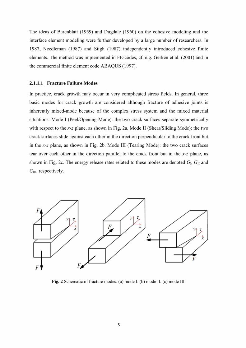
In practice, crack growth may occur in very complicated stress fields. In general, three

basic modes for crack growth are considered although fracture of adhesive joints is

inherently mixed-mode because of the complex stress system and the mixed material

situations. Mode I (Peel/Opening Mode): the two crack surfaces separate symmetrically

with respect to the x-z plane, as shown in Fig. 2a. Mode II (Shear/Sliding Mode): the two

crack surfaces slide against each other in the direction perpendicular to the crack front but

in the x-z plane, as shown in Fig. 2b. Mode III (Tearing Mode): the two crack surfaces

tear over each other in the direction parallel to the crack front but in the x-z plane, as

shown in Fig. 2c. The energy release rates related to these modes are denoted GI, GII and

GIII, respectively.

Fig. 2 Schematic of fracture modes. (a) mode I. (b) mode II. (c) mode III.

6

2.1.1.2 Linear Elastic Fracture Mechanics

In the regime where the global stress-strain response is linear and elastic, the elastic

energy release rate, G, and the stress intensity factor K can be used for characterizing the

loading of cracks in structures.

In the energy approach of Linear Elastic Fracture Mechanics (LEFM), the fracture

behavior is described by the variation of the potential energy due to crack extension. This

is characterized by the energy release rate, G. The energy release rate is defined as the

decrease of the total potential energy with respect to crack extension under constant load,

that is

dd

Ga

where a is the crack length and Π is the total potential energy per unit thickness of

system. Thus, in fracture mechanics, the total potential energy is the source for crack

growth. Accordingly, an energy criterion for the onset of crack growth is defined in the

following general form:

c c2G G

In which G is known as the crack driving force, and c is the surface energy per unit area

of the crack.

The energy release rate, G, can be considered as the energy source for crack growth. It

can be obtained from a stress analysis of the cracked body if the inelastic behavior of the

crack tip can be neglected. On the other hand, the surface energy, c , can be considered

as the energy sink and depends on many factors including the chemical composition and

microstructure of the material, temperature, environment and loading rate. The

experimentally measured critical energy release rate, Gc, for engineering materials,

specifically metals, is significantly larger than c2 and this is because plastic deformation

in the crack tip region also contributes significantly to the crack growth resistance. For a

perfectly brittle solid (NaCl single crystal), it has been shown that Gc= c2 is valid, cf.

e.g. Sun and Jin (2011).

7

2.1.1.3 Mixed Mode Failure Criteria

Failure criteria for mixed-mode fracture can be developed in a way analogous to the

classical failure criteria. Various mathematical fracture surfaces have been proposed to fit

the experimental results, such as:

I II III

Ic IIc IIc

1G G GG G G

where IcG , IIcG and IIIcG are the fracture toughness under pure mode I, II and III of

loading, respectively. The linear energetic criterion ( 1 ) and the quadratic one ( 2 )

are the most used. The exponents may be chosen to form the best fit of experimental data

or may be prescribed based on some assumed relationship, cf. e.g. Sun and Jin (2011).

2.1.1.4 Nonlinear Fracture Mechanics

When a crack occurs in a ductile body, a plastic region appears in the vicinity of the crack

tip. If the size of this plastic region is substantial, G cannot be determined from the elastic

stress field, since G may be affected by the crack tip plastic zone (e.g. Forman, 1967). In

1951, Eshelby introduced the concept of the force on a singularity and derived a path

independent integral, cf. Fig. 3. In 1968 Rice applied this integral to crack problems and

denoted it the J-integral. J is the release of potential energy for a virtual crack extension

da per unit width of the crack front.

Because the J-integral is applicable for infinite as well as finite applications,

homogeneous as well as inhomogeneous, linear as well as non-linear materials, it is a

very powerful tool for determining the crack extension force, cf. Weinberger et al.

(2005). For a linear elastic material J=G but J remains the energy release rate for a

nonlinear elastic material. Thus, one can postulate that a crack grows if J exceeds a

critical value Jc which is analogous to Gc and equals to Gc if LEFM can be applied.

In two dimensional problems, the J-integral is written for a crack along x direction as

d dii

uJ W y Tx

(1)

8

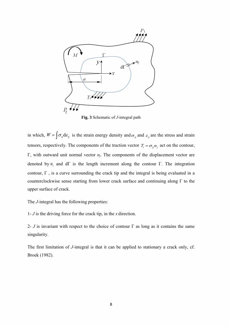
Fig. 3 Schematic of J-integral path

in which, dij ijW is the strain energy density and ij and ij are the stress and strain

tensors, respectively. The components of the traction vector i ij jT n act on the contour,

Г, with outward unit normal vector nj. The components of the displacement vector are

denoted by iu and dГ is the length increment along the contour Г. The integration

contour, Г , is a curve surrounding the crack tip and the integral is being evaluated in a

counterclockwise sense starting from lower crack surface and continuing along Г to the

upper surface of crack.

The J-integral has the following properties:

1- J is the driving force for the crack tip, in the x direction.

2- J is invariant with respect to the choice of contour Г as long as it contains the same

singularity.

The first limitation of J-integral is that it can be applied to stationary a crack only, cf.

Broek (1982).

9

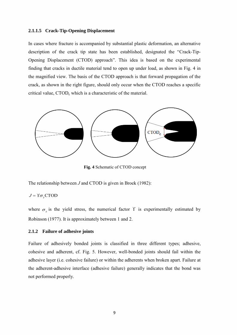
2.1.1.5 Crack-Tip-Opening Displacement

In cases where fracture is accompanied by substantial plastic deformation, an alternative

description of the crack tip state has been established, designated the “Crack-Tip-

Opening Displacement (CTOD) approach”. This idea is based on the experimental

finding that cracks in ductile material tend to open up under load, as shown in Fig. 4 in

the magnified view. The basis of the CTOD approach is that forward propagation of the

crack, as shown in the right figure, should only occur when the CTOD reaches a specific

critical value, CTODc which is a characteristic of the material.

Fig. 4 Schematic of CTOD concept

The relationship between J and CTOD is given in Broek (1982):

yCTODJ

where y is the yield stress, the numerical factor is experimentally estimated by

Robinson (1977). It is approximately between 1 and 2.

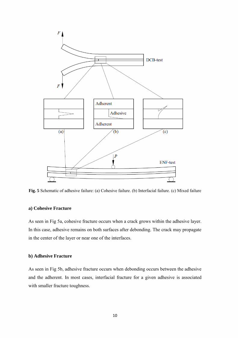
2.1.2 Failure of adhesive joints

Failure of adhesively bonded joints is classified in three different types; adhesive,

cohesive and adherent, cf. Fig. 5. However, well-bonded joints should fail within the

adhesive layer (i.e. cohesive failure) or within the adherents when broken apart. Failure at

the adherent-adhesive interface (adhesive failure) generally indicates that the bond was

not performed properly.

10

Fig. 5 Schematic of adhesive failure: (a) Cohesive failure. (b) Interfacial failure. (c) Mixed failure

a) Cohesive Fracture

As seen in Fig 5a, cohesive fracture occurs when a crack grows within the adhesive layer.

In this case, adhesive remains on both surfaces after debonding. The crack may propagate

in the center of the layer or near one of the interfaces.

b) Adhesive Fracture

As seen in Fig 5b, adhesive fracture occurs when debonding occurs between the adhesive

and the adherent. In most cases, interfacial fracture for a given adhesive is associated

with smaller fracture toughness.

11

c) Other types of fracture

Mixed types occur if the crack propagates at some spots in a cohesive and in other spots in

an adhesive manner, cf. Fig. 5c. Mixed fracture surfaces can be characterized by a certain

percentage of adhesive and cohesive areas. The alternating crack path type occurs if the

crack jumps from one interface to the other. This type of fracture appears in the presence

of tensile in-plane pre-stresses in the adhesive layer, cf. e.g. Fleck et al. (1991). Fracture

can also occur in the adherent if the adhesive is tougher than the adherent. In this case, the

adhesive remains intact and is still bonded to the adherents. For example, when one

removes a price label, the adhesive usually remains on the label and the surface. This is

cohesive failure. Although a layer of paper remains stuck to the surface, the adhesive has

not failed.

12

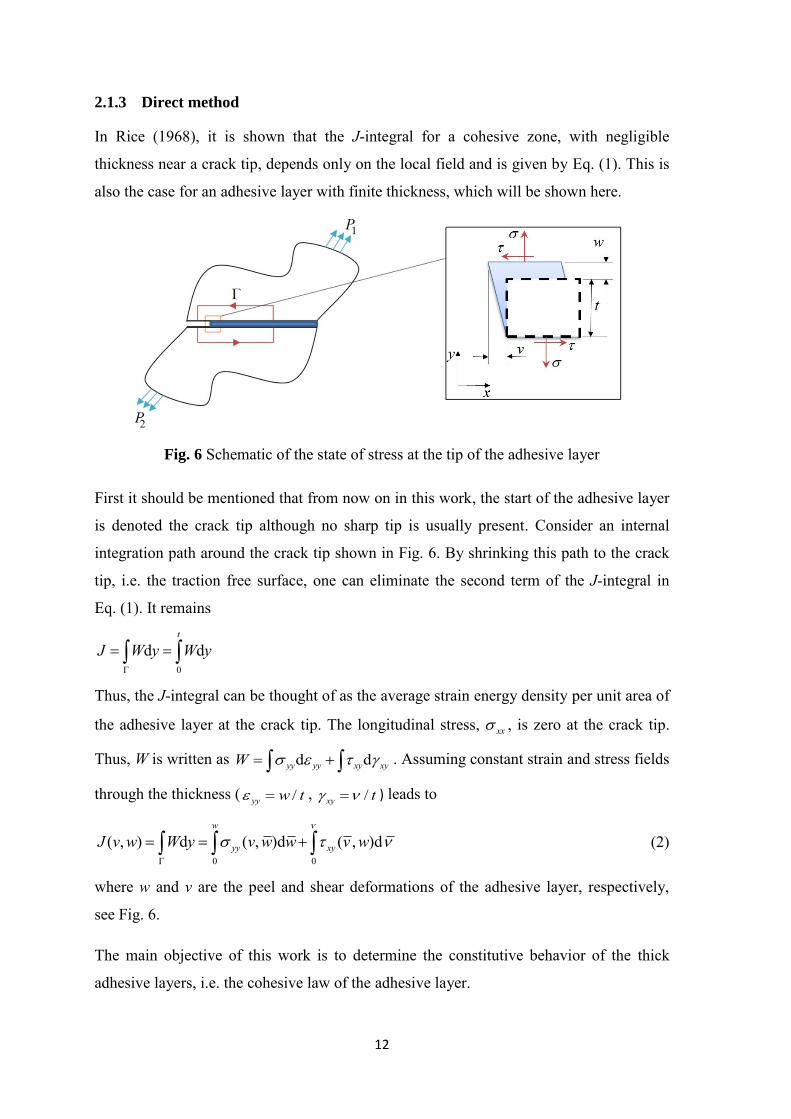
2.1.3 Direct method

In Rice (1968), it is shown that the J-integral for a cohesive zone, with negligible

thickness near a crack tip, depends only on the local field and is given by Eq. (1). This is

also the case for an adhesive layer with finite thickness, which will be shown here.

Fig. 6 Schematic of the state of stress at the tip of the adhesive layer

First it should be mentioned that from now on in this work, the start of the adhesive layer

is denoted the crack tip although no sharp tip is usually present. Consider an internal

integration path around the crack tip shown in Fig. 6. By shrinking this path to the crack

tip, i.e. the traction free surface, one can eliminate the second term of the J-integral in

Eq. (1). It remains

0

d dt

J W y W y

Thus, the J-integral can be thought of as the average strain energy density per unit area of

the adhesive layer at the crack tip. The longitudinal stress, xx , is zero at the crack tip.

Thus, W is written as d dyy yy xy xyW . Assuming constant strain and stress fields

through the thickness ( /yy w t , /xy t ) leads to

0 0

( , ) d ( , )d ( , )dw

yy xyJ v w W y v w w v w

(2)

where w and v are the peel and shear deformations of the adhesive layer, respectively,

see Fig. 6.

The main objective of this work is to determine the constitutive behavior of the thick

adhesive layers, i.e. the cohesive law of the adhesive layer.

13

By the direct method, the complete cohesive law for a given adhesive can be measured by

differentiation of the J-v or J-w curves. A few works currently exist on the direct

parameter determination of adhesive bonds (Sørensen, 2002) and fiber reinforced

composites (Sørensen and Jacobsen, 2003). Andersson and Stigh (2004) use an direct

method to determine the cohesive parameters in peel mode of loading for a ductile

adhesive bond in DCB test configuration. Leffler et al. (2007) use a similar method to

measure the cohesive parameters in shear loading of a ductile adhesive bond using an

ENF test configuration.

Shear and peel deformations at the crack tip (v, w) and J are measured during the

experiments. To this end, having an expression for J in terms of measurable parameters is

needed for each test configuration. These kinds of expressions are derived in the next

sections. To determine the cohesive law, the differentiation of J with respect to v and w

needs to be taken as follows

( , ) Jw vw

, ( , ) Jw vv

(3)

These differentiations of experimental data J(v, w) might cause a substantial scatter. In

order to minimize the scatter, we first fit a polynomial of order k to the experimental J-v

and J-w curves. Then the differentiation with respect to v and w are taken. The

polynomial-series are given by

0

ki

ii

J w A w

, 0

ki

ii

J v Av

The alternative method is to fit a Prony-series with k terms to the experimental J-v and J-

w curves and then differentiate with respect to v and w. The Prony-series are given by

1 c

expk

ii

kwJ w Aiw

,

1 c

expk

ii

kvJ v Aiv

The parameters Ai of both types of series are determined by a least square fit procedure.

The choice of the number of terms, k, in both cases, is made based by visual comparison

of the fitted and experimental curves, cf. Fig. 7.

14

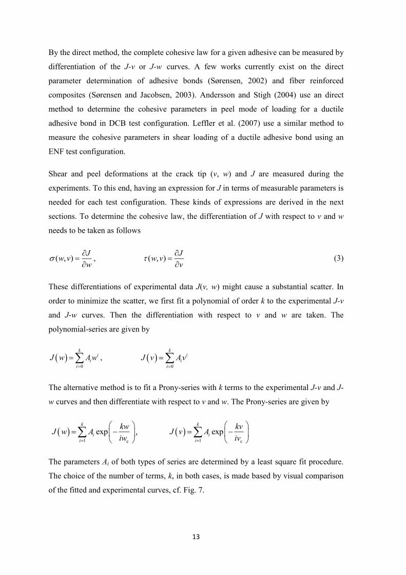
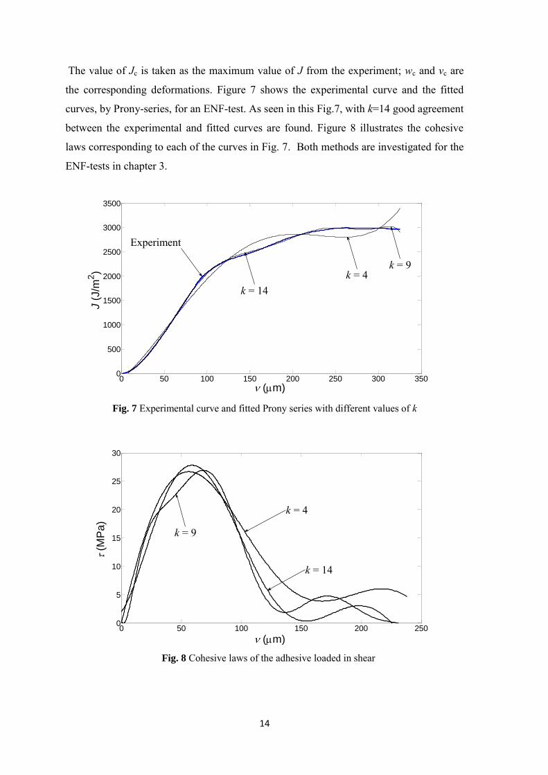
The value of Jc is taken as the maximum value of J from the experiment; wc and vc are

the corresponding deformations. Figure 7 shows the experimental curve and the fitted

curves, by Prony-series, for an ENF-test. As seen in this Fig.7, with k=14 good agreement

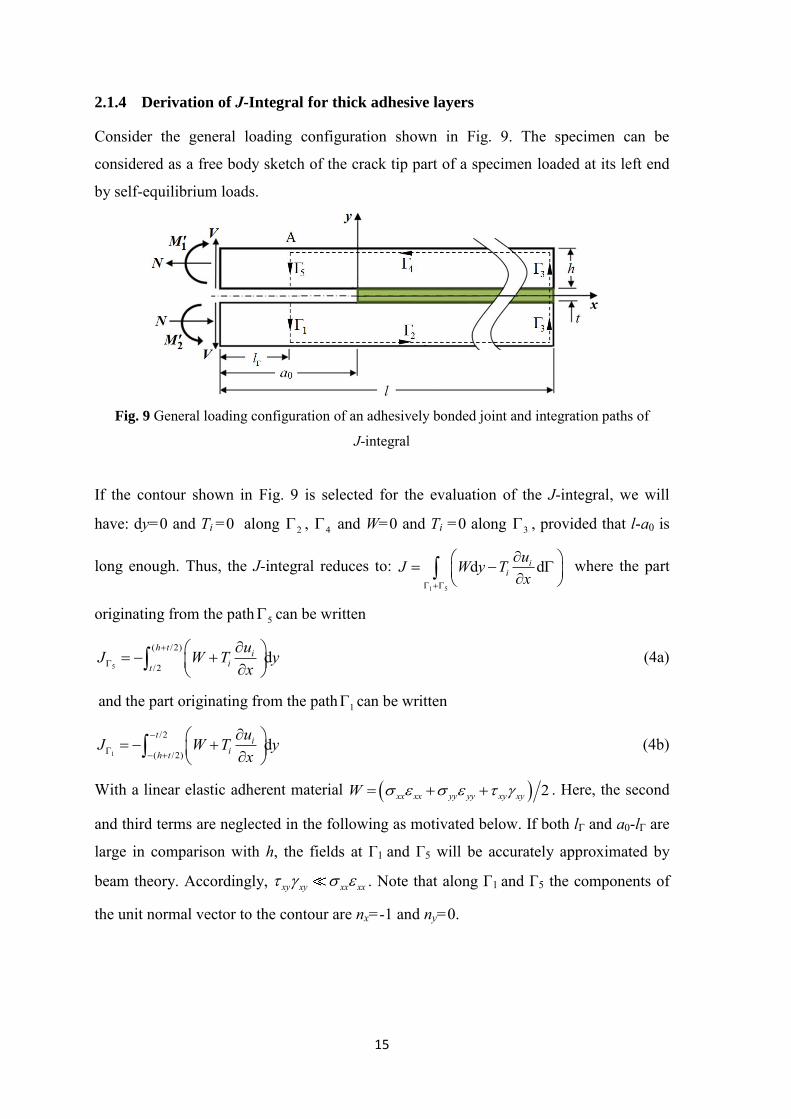
between the experimental and fitted curves are found. Figure 8 illustrates the cohesive

laws corresponding to each of the curves in Fig. 7. Both methods are investigated for the

ENF-tests in chapter 3.

Fig. 7 Experimental curve and fitted Prony series with different values of k

Fig. 8 Cohesive laws of the adhesive loaded in shear

0 50 100 150 200 250 300 3500

500

1000

1500

2000

2500

3000

3500

(m)

J (

J/m

2)

k = 14k = 4

k = 9

Experiment

0 50 100 150 200 2500

5

10

15

20

25

30

(m)

(M

Pa)

k = 9

k = 4

k = 14

15

2.1.4 Derivation of J-Integral for thick adhesive layers

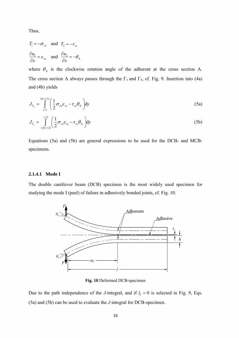
Consider the general loading configuration shown in Fig. 9. The specimen can be

considered as a free body sketch of the crack tip part of a specimen loaded at its left end

by self-equilibrium loads.

Fig. 9 General loading configuration of an adhesively bonded joint and integration paths of

J-integral

If the contour shown in Fig. 9 is selected for the evaluation of the J-integral, we will

have: dy=0 and Ti =0 along 2 , 4 and W=0 and Ti =0 along 3 , provided that l-a0 is

long enough. Thus, the J-integral reduces to: 1 5

d dii

uJ W y Tx

where the part

originating from the path 5 can be written

5

( /2)

/2d

h t iit

uJ W T yx

(4a)

and the part originating from the path 1 can be written

1

/2

( /2)d

t iih t

uJ W T yx

(4b)

With a linear elastic adherent material 2xx xx yy yy xy xyW . Here, the second

and third terms are neglected in the following as motivated below. If both lΓ and a0-lΓ are

large in comparison with h, the fields at Γ1 and Γ5 will be accurately approximated by

beam theory. Accordingly, xy xy xx xx . Note that along Γ1 and Γ5 the components of

the unit normal vector to the contour are nx=-1 and ny=0.

16

Thus,

1 xxT and 2 xyT

1xx

ux

and 2A

ux

where A is the clockwise rotation angle of the adherent at the cross section A.

The cross section A always passes through the Γ1 and Γ5, cf. Fig. 9. Insertion into (4a)

and (4b) yields

5

( /2)

A/2

1 d2

h t

xx xx xyt

J y

(5a)

1

/2

A( /2)

1 d2

t

xx xx xyh t

J y

(5b)

Equations (5a) and (5b) are general expressions to be used for the DCB- and MCB-

specimens.

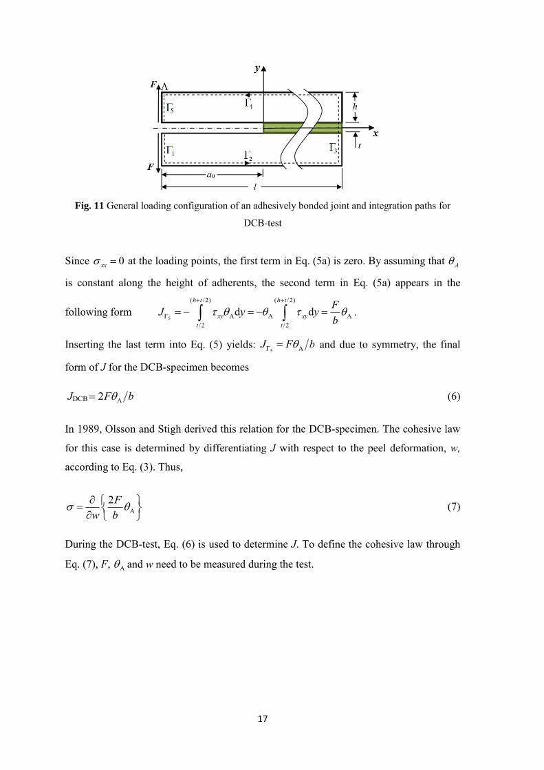
2.1.4.1 Mode I

The double cantilever beam (DCB) specimen is the most widely used specimen for

studying the mode I (peel) of failure in adhesively bonded joints, cf. Fig. 10.

Fig. 10 Deformed DCB-specimen

Due to the path independence of the J-integral, and if 0l is selected in Fig. 9, Eqs.

(5a) and (5b) can be used to evaluate the J-integral for DCB-specimen.

17

Fig. 11 General loading configuration of an adhesively bonded joint and integration paths for

DCB-test

Since 0xx at the loading points, the first term in Eq. (5a) is zero. By assuming that A

is constant along the height of adherents, the second term in Eq. (5a) appears in the

following form 5

( /2) ( /2)

A A A/2 /2

d dh t h t

xy xyt t

FJ y yb

.

Inserting the last term into Eq. (5) yields: 5 AJ F b and due to symmetry, the final

form of J for the DCB-specimen becomes

JDCB A2F b (6)

In 1989, Olsson and Stigh derived this relation for the DCB-specimen. The cohesive law

for this case is determined by differentiating J with respect to the peel deformation, w,

according to Eq. (3). Thus,

A2F

w b

(7)

During the DCB-test, Eq. (6) is used to determine J. To define the cohesive law through

Eq. (7), F, A and w need to be measured during the test.

18

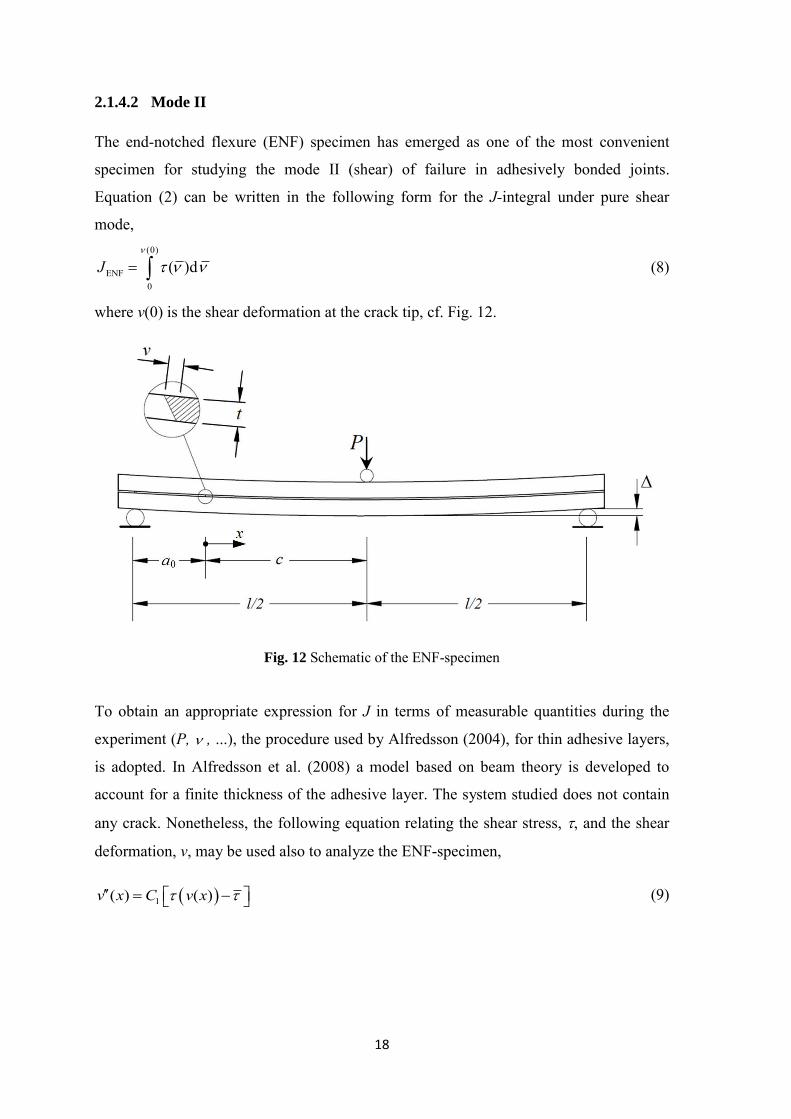
2.1.4.2 Mode II

The end-notched flexure (ENF) specimen has emerged as one of the most convenient

specimen for studying the mode II (shear) of failure in adhesively bonded joints.

Equation (2) can be written in the following form for the J-integral under pure shear

mode, (0)

ENF0

( )dJ

(8)

where v(0) is the shear deformation at the crack tip, cf. Fig. 12.

Fig. 12 Schematic of the ENF-specimen

To obtain an appropriate expression for J in terms of measurable quantities during the

experiment (P, , ...), the procedure used by Alfredsson (2004), for thin adhesive layers,

is adopted. In Alfredsson et al. (2008) a model based on beam theory is developed to

account for a finite thickness of the adhesive layer. The system studied does not contain

any crack. Nonetheless, the following equation relating the shear stress, , and the shear

deformation, v, may be used also to analyze the ENF-specimen,

1( ) ( )v x C v x (9)

19

where 2

18 3 31

2 4t tC

Eh h h

and where E is the elastic modulus of the beam material. In Eq. (9), is the shear stress

predicted by ordinary beam theory,

2

138 3 31

2 4

tP hbh t t

h h

(10)

where P is the applied force, t is the thickness of adhesive layer, h is the thickness of

adherents, b is the specimen’s width.

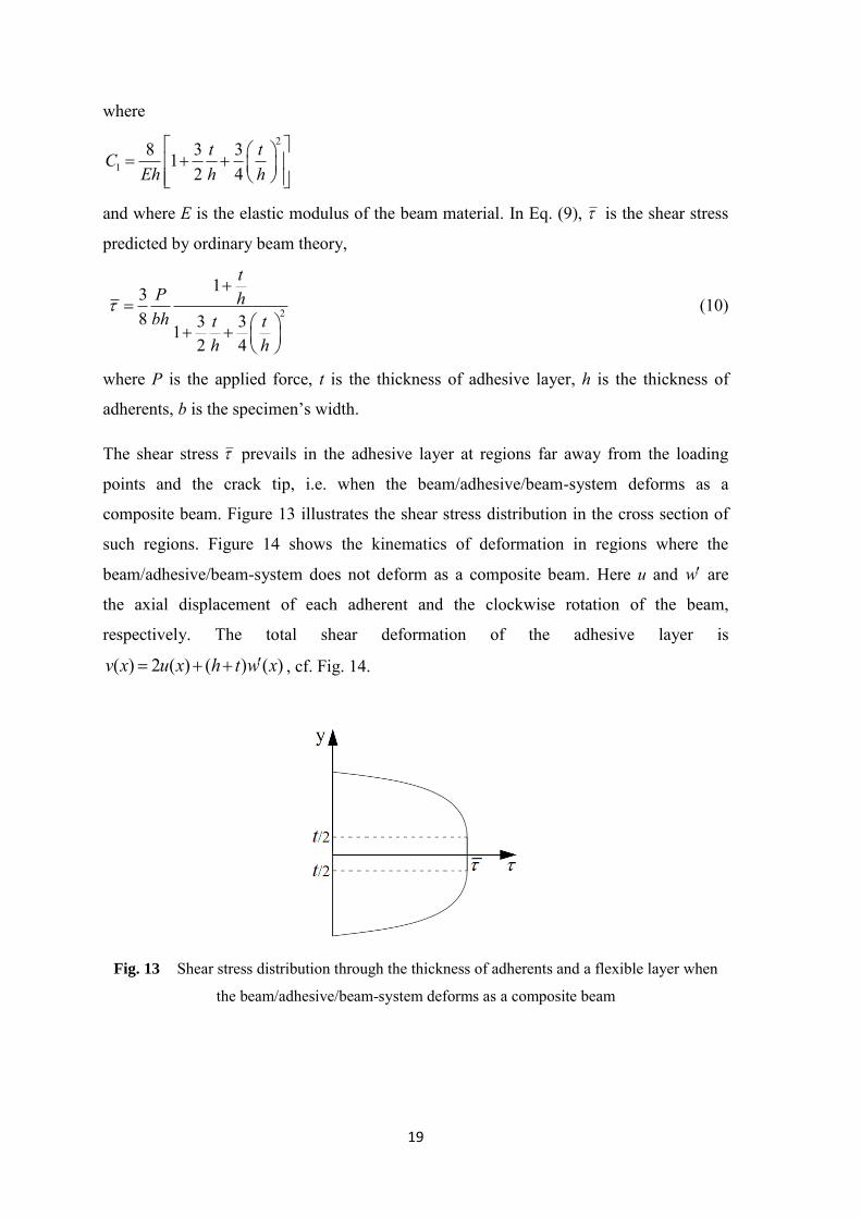
The shear stress prevails in the adhesive layer at regions far away from the loading

points and the crack tip, i.e. when the beam/adhesive/beam-system deforms as a

composite beam. Figure 13 illustrates the shear stress distribution in the cross section of

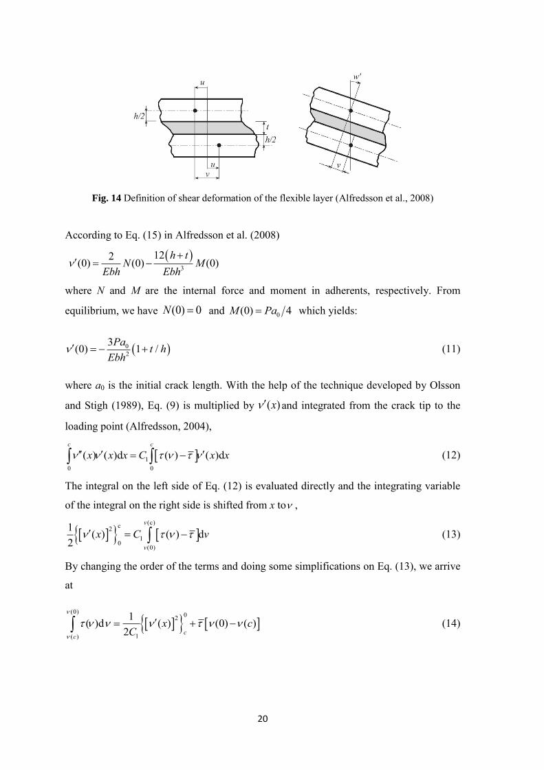
such regions. Figure 14 shows the kinematics of deformation in regions where the

beam/adhesive/beam-system does not deform as a composite beam. Here u and w are

the axial displacement of each adherent and the clockwise rotation of the beam,

respectively. The total shear deformation of the adhesive layer is

( ) 2 ( ) ( ) ( )v x u x h t w x , cf. Fig. 14.

Fig. 13 Shear stress distribution through the thickness of adherents and a flexible layer when

the beam/adhesive/beam-system deforms as a composite beam

20

Fig. 14 Definition of shear deformation of the flexible layer (Alfredsson et al., 2008)

According to Eq. (15) in Alfredsson et al. (2008)

3

122(0) (0) (0)h t

N MEbh Ebh

where N and M are the internal force and moment in adherents, respectively. From

equilibrium, we have (0) 0N and 0(0) 4M Pa which yields:

02

3(0) 1 /Pa t hEbh

(11)

where a0 is the initial crack length. With the help of the technique developed by Olsson

and Stigh (1989), Eq. (9) is multiplied by ( )x and integrated from the crack tip to the

loading point (Alfredsson, 2004),

10 0

( ) ( )d ( ) ( )dc c

x x x C x x

(12)

The integral on the left side of Eq. (12) is evaluated directly and the integrating variable

of the integral on the right side is shifted from x to ,

(c)c2

10

(0)

1 ( ) ( ) d2

v

v

x C v

(13)

By changing the order of the terms and doing some simplifications on Eq. (13), we arrive

at

(0) 02

1( )

1( )d ( ) (0) ( )2 c

c

x cC

(14)

21

Using Eq. (8), the energy release rate is identified as

( )

2 2ENF

10

1( )d (0) ( ) (0) ( )2

c

J c cC

Inserting the boundary conditions from Eq. (11) and from Eq. (10), the ERR appears in

the following form:

2

( )2 220

ENF 2 22 31 0

1 19 3 1 ( ) ( )d16 8 23 3 3 31 1

2 4 2 4

ct t

P a Pvh hJ cEb h bh Ct t t t

h h h h

(15)

where v = v(0) is the shear deformation of the adhesive at the crack tip and ( )c is the

shear deformation of the adhesive at the loading point, cf. Fig. 12.

For specimens long enough to ensure that the shear deformation at the loading point is

small, ( ) (0)c and ( ) (0)c , the last two terms in Eq. (15) can be neglected.

In this case we have,

ENF 0 1J J J (16)

where

2

2 20

0 2 2 3

19

163 312 4

tP ahJEb ht t

h h

and 1 2

1 383 31

2 4

tPhJbht t

h h

.

The stress-deformation relation for shear is obtained by differentiating of J with respect

to the shear deformation, v.

2 2

22 3

19 31

16 8 3 312 4

tP a t P hEb h h bh t t

h h

(17)

Equation (17) is a generalized relation of the previous results by Alfredsson (2004) and

Leffler et al. (2007), accounting for a finite thickness of the adhesive layer. To measure

the cohesive law through the Eq. (17), P and v need to be measured during an experiment.

22

2.1.4.3 Mixed-mode

Various attempts have been made to characterize the fracture toughness under mixed-

mode loading conditions in adhesively bonded joints, where mostly beam type specimens

have been used (Sørensen and Kirkegaard, 2006; Högberg et al., 2007; and Choupani,

2008). The mixed-mode cantilever beam (MCB) test specimen developed by Högberg et

al. (2007) is used to study the mixed-mode fracture of adhesively bonded joints in this

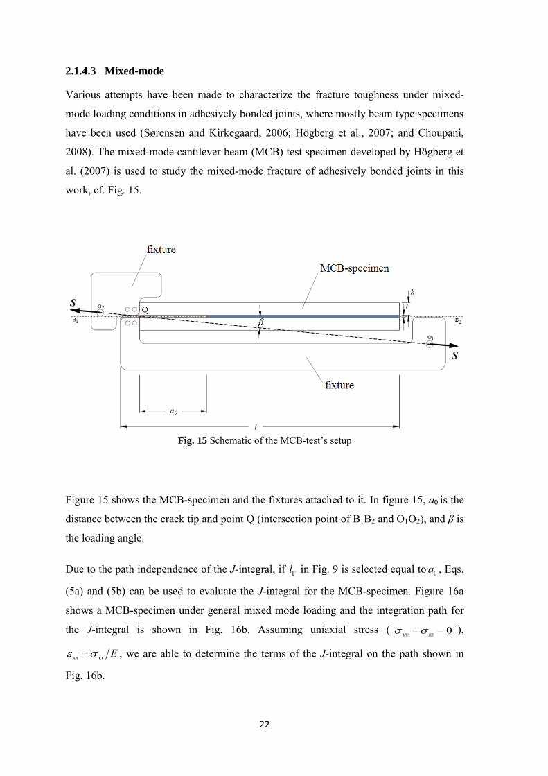
work, cf. Fig. 15.

Fig. 15 Schematic of the MCB-test’s setup

Figure 15 shows the MCB-specimen and the fixtures attached to it. In figure 15, a0 is the

distance between the crack tip and point Q (intersection point of B1B2 and O1O2), and β is

the loading angle.

Due to the path independence of the J-integral, if l in Fig. 9 is selected equal to 0a , Eqs.

(5a) and (5b) can be used to evaluate the J-integral for the MCB-specimen. Figure 16a

shows a MCB-specimen under general mixed mode loading and the integration path for

the J-integral is shown in Fig. 16b. Assuming uniaxial stress ( 0yy zz ),

xx xx E , we are able to determine the terms of the J-integral on the path shown in

Fig. 16b.

23

(a)

(b)

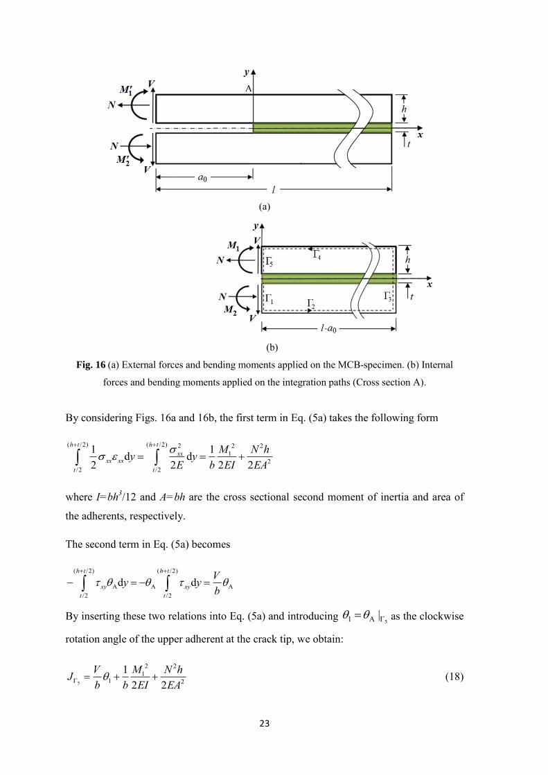
Fig. 16 (a) External forces and bending moments applied on the MCB-specimen. (b) Internal

forces and bending moments applied on the integration paths (Cross section A).

By considering Figs. 16a and 16b, the first term in Eq. (5a) takes the following form

( /2) ( /2) 2 2 21

2/2 /2

1 1d d2 2 2 2

h t h txx

xx xxt t

M N hy yE b EI EA

where I=bh3/12 and A=bh are the cross sectional second moment of inertia and area of

the adherents, respectively.

The second term in Eq. (5a) becomes

( /2) ( /2)

A A A/2 /2

d dh t h t

xy xyt t

Vy yb

By inserting these two relations into Eq. (5a) and introducing 51 A | as the clockwise

rotation angle of the upper adherent at the crack tip, we obtain:

5

2 21

1 2

12 2MV N hJ

b b EI EA

(18)

24

In a similar fashion, by using Eq. (5b) and assuming that 12 A | is the clockwise

rotation angle of the lower adherent at the crack tip, we obtain 1

J for lower adherent

1

2 22

2 2

12 2MV N hJ

b b EI EA

By adding 5

J and

1J

the total J for MCB specimen appears in the following form

JMCB 2 2 2

1 21 2 2 3 2

6( )M MV Nb Eb h Eb h

(19)

From equilibrium, the cross-sectional forces and moments at the crack tip, cf. Figs. 15

and 16a, are given by

sinV S , cosN S , 1,2 0 2h tM Va N

(20)

where S is the applied force with angle with respect to the x-axis and h is the thickness

of adherent and t is the thickness of adhesive layer, see Fig. 15.

By inserting Eq. (20) into Eq. (19), we finally arrive at

JMCB

2 2 220

1 2 2 3 2

12 sin 4 cossin 3 3( ) 12 4

S a SS t tb Eb h Eb h h h

(21)

Thus, measurement of the applied force, S, and the rotational angles, 1 and 2 , are

required to experimentally determine J.

25

2.2 Rivet joints

2.2.1 Introduction

In engineering practice it is often required that two sheets or plates are joined together

and carry the load. Many times such joints are required to be leak proof so that gas

contained inside is not allowed to escape. A rivet joint is easily conceived between two

plates overlapping at edges, making holes through thickness of both, passing the stem of

rivet through holes and creating the head at the end of the stem on the other side. Such

joints have been used in structures, boilers and ships. Riveting is also a widely used

joining technology in the automotive and aerospace industries.

General failure models to predict the fracture behavior of joints made by riveting are

needed by designers but have not yet been developed. Accurate prediction of stresses

within and around a joint is a fundamental step in estimating the structural strength of

joints. A major difficulty in modeling rivet joints is how to idealize the load transfer

between the rivet and the plates. The resulting stress distribution around the rivet holes is

largely influenced by this idealization. Such predictions require both suitable failure

criteria and a method for implementing these criteria into numerical calculations. Both

strength-based and energy-based failure criteria are used for predicting the performance

of rivet joints. However, the use of a fracture mechanics based failure criteria is not

appropriate unless the scale of plastic deformation in a structure is much smaller than any

characteristic length. Owing to large-scale plasticity that accompanies fracture, this

condition is generally violated with any riveted sheet metal. Fracture problems in which

plastic deformation is significant can be analyzed by the use of cohesive-zone models that

incorporate both strength and energy criteria for fracture.

This thesis provides a novel approach of using cohesive modeling for analyzing riveted

structures in predicting the strength of rivet joints. The cohesive zone modeling within

finite element calculations is used to capture the fracture and failure load of rivet joints.

This technique uses two material parameters, cohesive strength and toughness, to

characterize the failure behavior of the joints under each mode of loading.

26

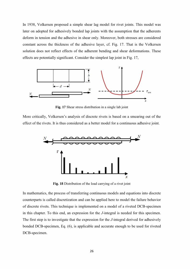
In 1938, Volkersen proposed a simple shear lag model for rivet joints. This model was

later on adopted for adhesively bonded lap joints with the assumption that the adherents

deform in tension and the adhesive in shear only. Moreover, both stresses are considered

constant across the thickness of the adhesive layer, cf. Fig. 17. That is the Volkersen

solution does not reflect effects of the adherent bending and shear deformations. These

effects are potentially significant. Consider the simplest lap joint in Fig. 17,

Fig. 17 Shear stress distribution in a single lab joint

More critically, Volkersen’s analysis of discrete rivets is based on a smearing out of the

effect of the rivets. It is thus considered as a better model for a continuous adhesive joint.

Fig. 18 Distribution of the load carrying of a rivet joint

In mathematics, the process of transferring continuous models and equations into discrete

counterparts is called discretization and can be applied here to model the failure behavior

of discrete rivets. This technique is implemented on a model of a riveted DCB-specimen

in this chapter. To this end, an expression for the J-integral is needed for this specimen.

The first step is to investigate that the expression for the J-integral derived for adhesively

bonded DCB-specimen, Eq. (6), is applicable and accurate enough to be used for riveted

DCB-specimen.

27

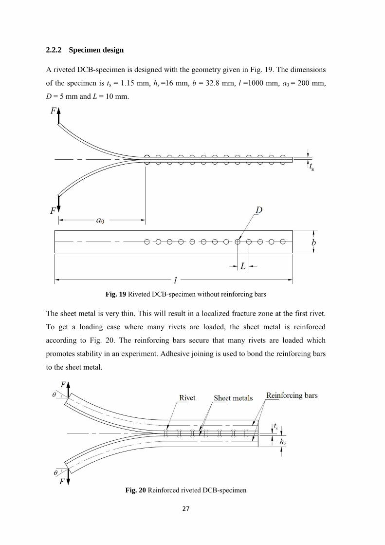
2.2.2 Specimen design

A riveted DCB-specimen is designed with the geometry given in Fig. 19. The dimensions

of the specimen is ts = 1.15 mm, hs =16 mm, b = 32.8 mm, l =1000 mm, a0 = 200 mm,

D = 5 mm and L = 10 mm.

Fig. 19 Riveted DCB-specimen without reinforcing bars

The sheet metal is very thin. This will result in a localized fracture zone at the first rivet.

To get a loading case where many rivets are loaded, the sheet metal is reinforced

according to Fig. 20. The reinforcing bars secure that many rivets are loaded which

promotes stability in an experiment. Adhesive joining is used to bond the reinforcing bars

to the sheet metal.

Fig. 20 Reinforced riveted DCB-specimen

28

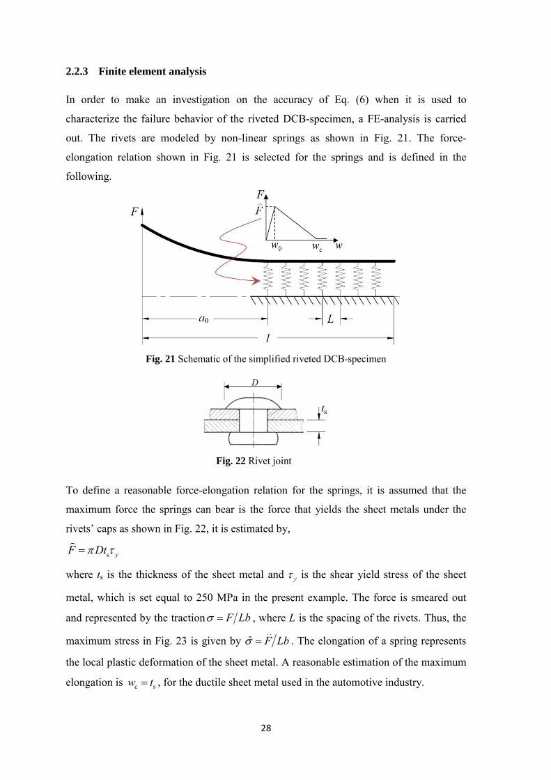
2.2.3 Finite element analysis

In order to make an investigation on the accuracy of Eq. (6) when it is used to

characterize the failure behavior of the riveted DCB-specimen, a FE-analysis is carried

out. The rivets are modeled by non-linear springs as shown in Fig. 21. The force-

elongation relation shown in Fig. 21 is selected for the springs and is defined in the

following.

Fig. 21 Schematic of the simplified riveted DCB-specimen

Fig. 22 Rivet joint

To define a reasonable force-elongation relation for the springs, it is assumed that the

maximum force the springs can bear is the force that yields the sheet metals under the

rivets’ caps as shown in Fig. 22, it is estimated by,

s yF Dt

where ts is the thickness of the sheet metal and y is the shear yield stress of the sheet

metal, which is set equal to 250 MPa in the present example. The force is smeared out

and represented by the traction F Lb , where L is the spacing of the rivets. Thus, the

maximum stress in Fig. 23 is given by ˆ F Lb . The elongation of a spring represents

the local plastic deformation of the sheet metal. A reasonable estimation of the maximum

elongation is c sw t , for the ductile sheet metal used in the automotive industry.

29

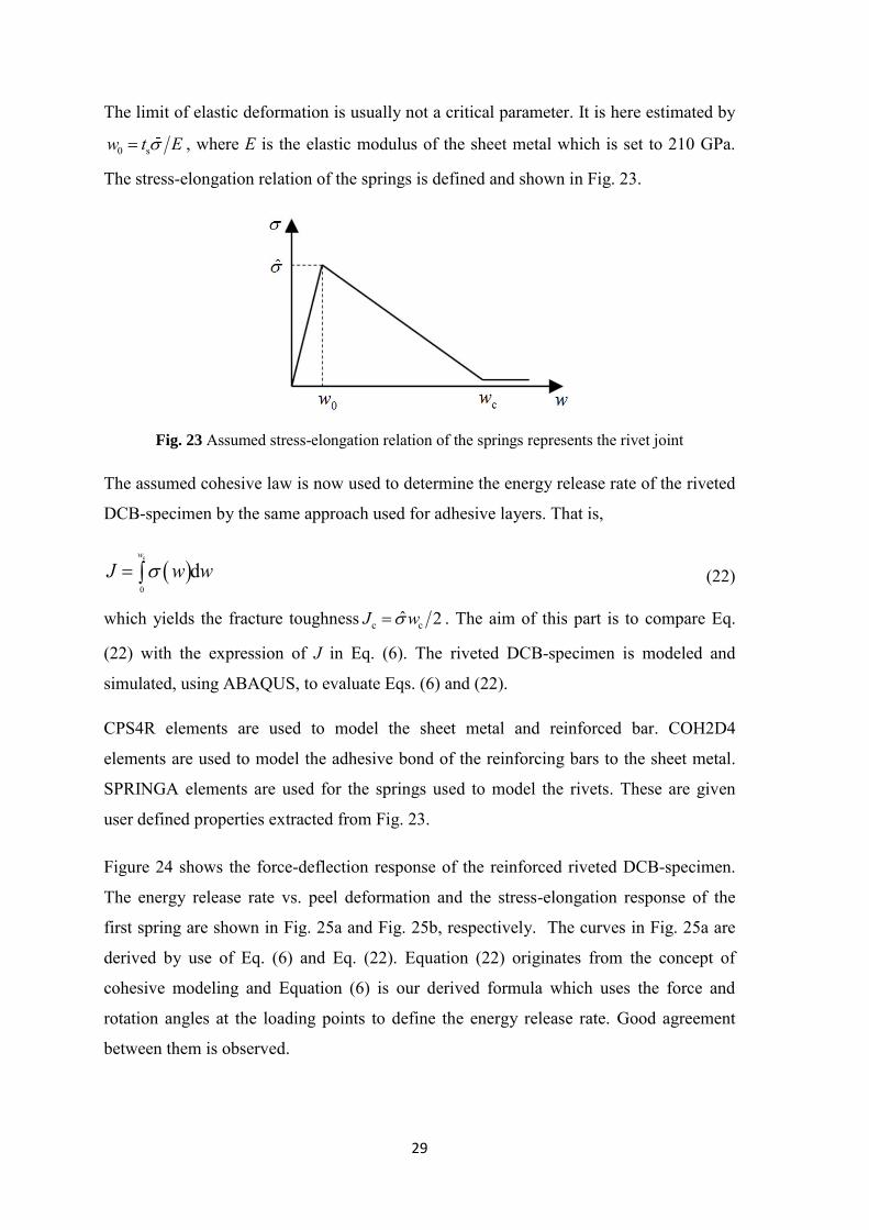
The limit of elastic deformation is usually not a critical parameter. It is here estimated by

0 sw t E , where E is the elastic modulus of the sheet metal which is set to 210 GPa. The stress-elongation relation of the springs is defined and shown in Fig. 23.

Fig. 23 Assumed stress-elongation relation of the springs represents the rivet joint

The assumed cohesive law is now used to determine the energy release rate of the riveted

DCB-specimen by the same approach used for adhesive layers. That is,

c

0

dw

J w w

(22)

which yields the fracture toughness c cˆ 2J w . The aim of this part is to compare Eq.

(22) with the expression of J in Eq. (6). The riveted DCB-specimen is modeled and

simulated, using ABAQUS, to evaluate Eqs. (6) and (22).

CPS4R elements are used to model the sheet metal and reinforced bar. COH2D4

elements are used to model the adhesive bond of the reinforcing bars to the sheet metal.

SPRINGA elements are used for the springs used to model the rivets. These are given

user defined properties extracted from Fig. 23.

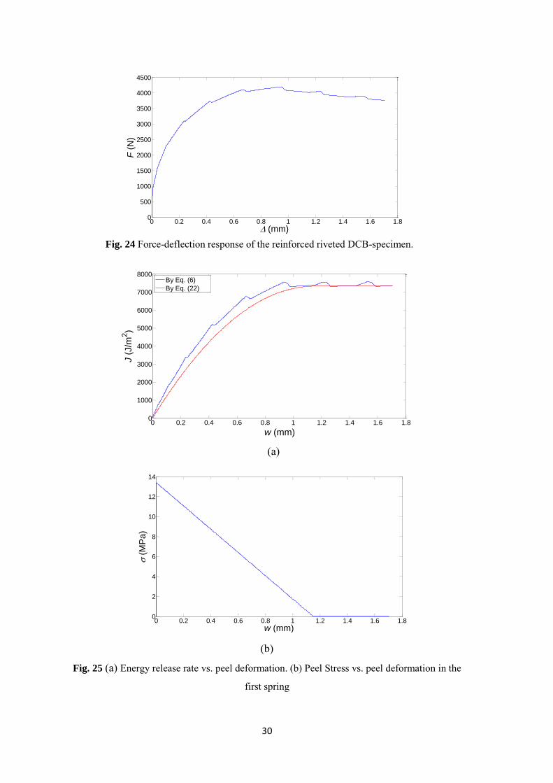
Figure 24 shows the force-deflection response of the reinforced riveted DCB-specimen.

The energy release rate vs. peel deformation and the stress-elongation response of the

first spring are shown in Fig. 25a and Fig. 25b, respectively. The curves in Fig. 25a are

derived by use of Eq. (6) and Eq. (22). Equation (22) originates from the concept of

cohesive modeling and Equation (6) is our derived formula which uses the force and

rotation angles at the loading points to define the energy release rate. Good agreement

between them is observed.

30

Fig. 24 Force-deflection response of the reinforced riveted DCB-specimen.

(a)

(b)

Fig. 25 (a) Energy release rate vs. peel deformation. (b) Peel Stress vs. peel deformation in the

first spring

0 0.2 0.4 0.6 0.8 1 1.2 1.4 1.6 1.80

500

1000

1500

2000

2500

3000

3500

4000

4500

(mm)

F (

N)

0 0.2 0.4 0.6 0.8 1 1.2 1.4 1.6 1.80

1000

2000

3000

4000

5000

6000

7000

8000

w (mm)

J (

J/m

2)

By Eq. (6)

By Eq. (22)

0 0.2 0.4 0.6 0.8 1 1.2 1.4 1.6 1.80

2

4

6

8

10

12

14

w (mm)

(

MP

a)

31

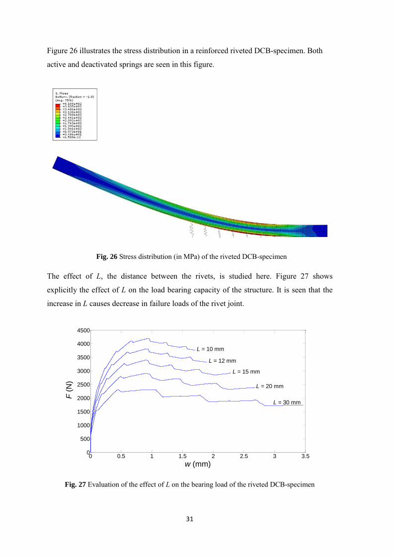
Figure 26 illustrates the stress distribution in a reinforced riveted DCB-specimen. Both

active and deactivated springs are seen in this figure.

Fig. 26 Stress distribution (in MPa) of the riveted DCB-specimen

The effect of L, the distance between the rivets, is studied here. Figure 27 shows

explicitly the effect of L on the load bearing capacity of the structure. It is seen that the

increase in L causes decrease in failure loads of the rivet joint.

Fig. 27 Evaluation of the effect of L on the bearing load of the riveted DCB-specimen

0 0.5 1 1.5 2 2.5 3 3.50

500

1000

1500

2000

2500

3000

3500

4000

4500

L = 10 mm

L = 12 mm

L = 15 mm

L = 20 mm

L = 30 mm

w (mm)

F (

N)

32

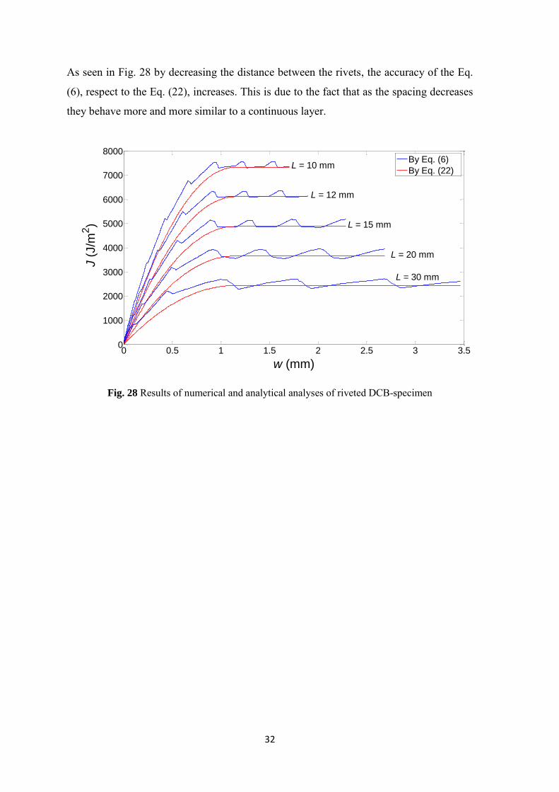
As seen in Fig. 28 by decreasing the distance between the rivets, the accuracy of the Eq.

(6), respect to the Eq. (22), increases. This is due to the fact that as the spacing decreases

they behave more and more similar to a continuous layer.

Fig. 28 Results of numerical and analytical analyses of riveted DCB-specimen

0 0.5 1 1.5 2 2.5 3 3.50

1000

2000

3000

4000

5000

6000

7000

8000

L = 10 mm

w (mm)

J (

J/m

2)

L = 12 mm

L = 15 mm

L = 20 mm

L = 30 mm

By Eq. (6)

By Eq. (22)

33

2.3 Cohesive zone modeling

2.3.1 Introduction

As discussed above, the concept of cohesive zone was proposed independently by

Barenblatt (1959, 1962) and Dugdale (1960) to describe damage under static loads at the

process zone ahead of the crack tip. Cohesive zone models were largely developed to

simulate crack initiation and propagation in cohesive and interfacial failure problems.

They are often modeled using nonlinear spring (e.g. Cui and Wisnom, 1993) or cohesive

finite elements (e.g. Mi et al., 1998). The concept of cohesive modeling is based on the

assumption that one or multiple fracture regions can be artificially introduced in

structures, in which damage growth is allowed by the introduction of a possible

discontinuity in the displacement field. The technique consists of the establishment of

traction–separation laws (addressed here as cohesive laws) to model interfaces or finite

regions. The cohesive laws are established between paired nodes of cohesive elements,

and they can be used to connect superimposed nodes of elements representing different

materials or different plies in composites, to simulate a zero thickness interface, or they

can be applied directly between two non-contacting materials to simulate a strip of finite

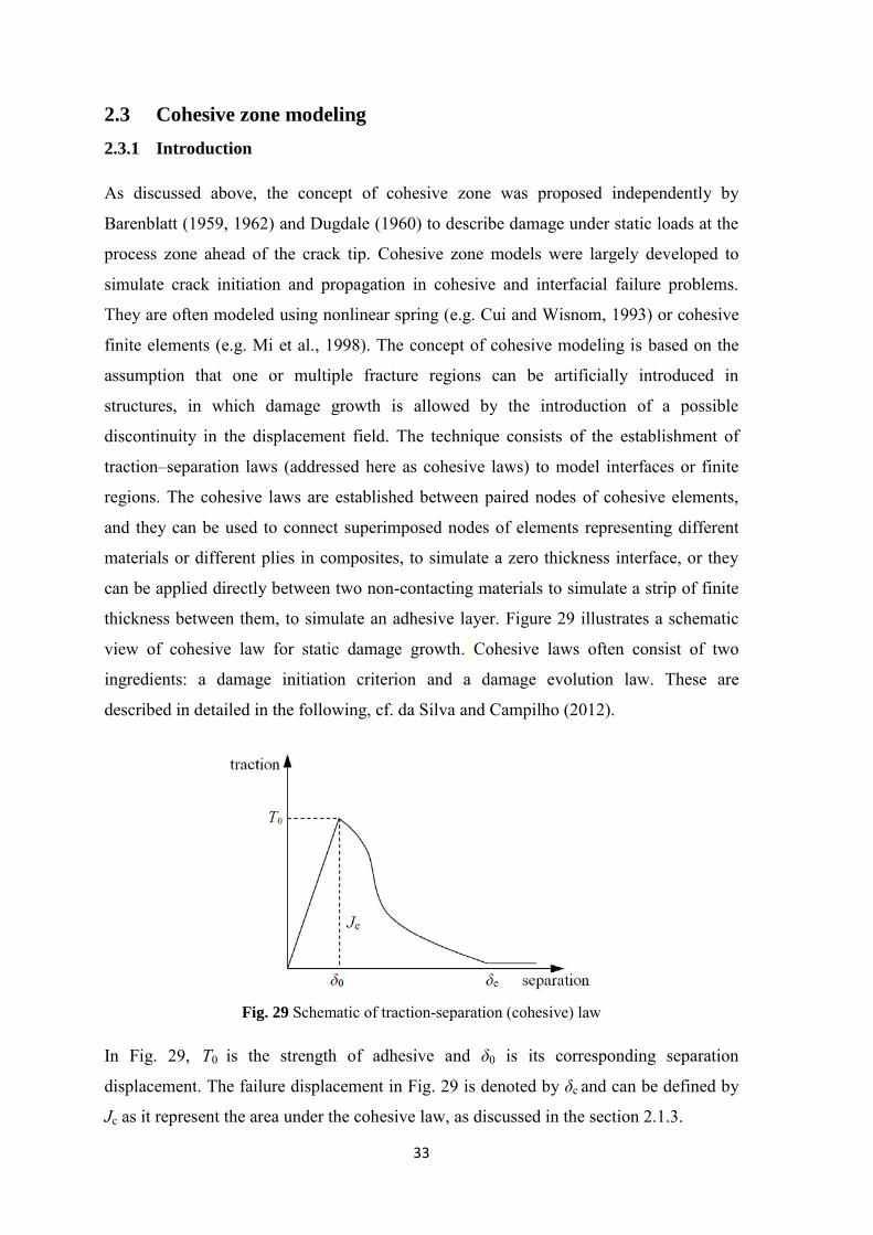
thickness between them, to simulate an adhesive layer. Figure 29 illustrates a schematic

view of cohesive law for static damage growth. Cohesive laws often consist of two

ingredients: a damage initiation criterion and a damage evolution law. These are

described in detailed in the following, cf. da Silva and Campilho (2012).

Fig. 29 Schematic of traction-separation (cohesive) law

In Fig. 29, T0 is the strength of adhesive and δ0 is its corresponding separation

displacement. The failure displacement in Fig. 29 is denoted by δc and can be defined by

Jc as it represent the area under the cohesive law, as discussed in the section 2.1.3.

34

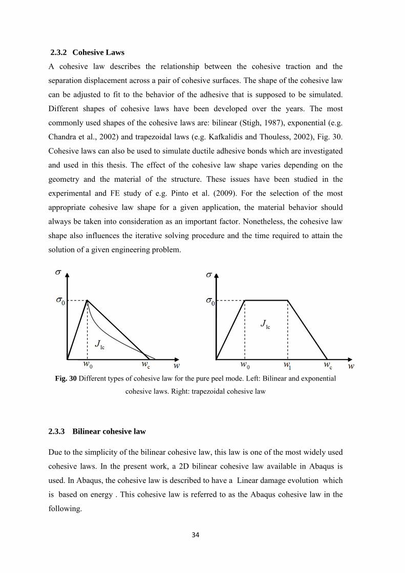
2.3.2 Cohesive Laws

A cohesive law describes the relationship between the cohesive traction and the

separation displacement across a pair of cohesive surfaces. The shape of the cohesive law

can be adjusted to fit to the behavior of the adhesive that is supposed to be simulated.

Different shapes of cohesive laws have been developed over the years. The most

commonly used shapes of the cohesive laws are: bilinear (Stigh, 1987), exponential (e.g.

Chandra et al., 2002) and trapezoidal laws (e.g. Kafkalidis and Thouless, 2002), Fig. 30.

Cohesive laws can also be used to simulate ductile adhesive bonds which are investigated

and used in this thesis. The effect of the cohesive law shape varies depending on the

geometry and the material of the structure. These issues have been studied in the

experimental and FE study of e.g. Pinto et al. (2009). For the selection of the most

appropriate cohesive law shape for a given application, the material behavior should

always be taken into consideration as an important factor. Nonetheless, the cohesive law

shape also influences the iterative solving procedure and the time required to attain the

solution of a given engineering problem.

Fig. 30 Different types of cohesive law for the pure peel mode. Left: Bilinear and exponential

cohesive laws. Right: trapezoidal cohesive law

2.3.3 Bilinear cohesive law

Due to the simplicity of the bilinear cohesive law, this law is one of the most widely used

cohesive laws. In the present work, a 2D bilinear cohesive law available in Abaqus is

used. In Abaqus, the cohesive law is described to have a Linear damage evolution which

is based on energy . This cohesive law is referred to as the Abaqus cohesive law in the

following.

35

In order to simplify the mathematical description, the total separation displacement, ,

and the direction variable, , are introduced as

2 2w v (23) 2

2 2

vw v

(24)

where w and v are the peel are shear deformations, respectively, cf. Fig. 6. For simplicity,

only non-negative v and w are considered in the following. Thus, the peel and shear

deformation can be expressed as

v , 1w (25)

For a deformation path with a fixed ratio v/w, i.e. with constant , the Abaqus cohesive

law displays bilinear response in terms of σ(w) and τ(v), cf. Fig. 31. For this type of

loading, the Abaqus cohesive law resembles the one presented by Camanho and Davila

(2002) but with different initial stiffnesses in peel and shear. The description of the

cohesive law provided in Abaqus’ manual is very brief, if not incomplete. Therefore, a

rather detailed description is given here as a generalization of the cohesive law given in

Camanho and Davila (2002). For a deformation path with constant , the described

cohesive law gives an identical response as the Abaqus cohesive law. However, for a

general loading path, the cohesive law described here differs from the cohesive law used

in Abaqus.

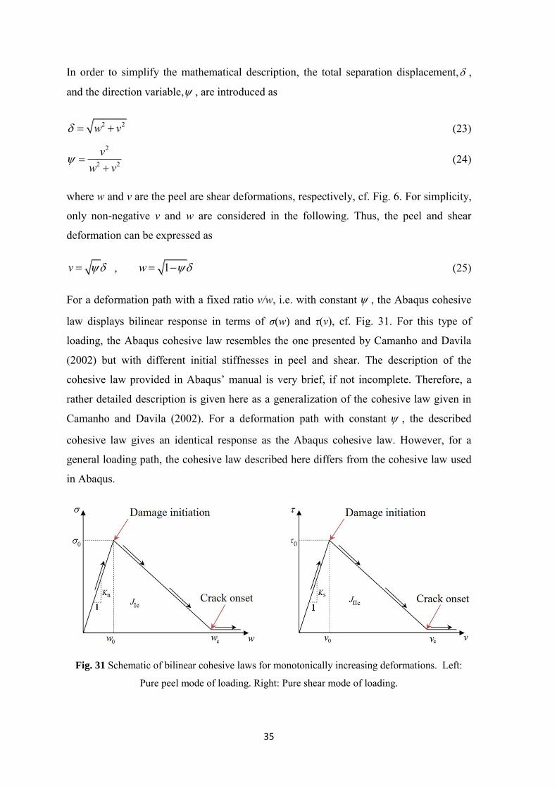
Fig. 31 Schematic of bilinear cohesive laws for monotonically increasing deformations. Left:

Pure peel mode of loading. Right: Pure shear mode of loading.

36

In Fig. 31, σ0 is the cohesive strength in the peel direction, w0 is the peel separation when

damage initiates, and wc is the peel displacement when decohesion occurs.

Correspondingly, τ0 is the cohesive strength in the shear direction, v0 is the shear

displacement when damage initiates and vc is the shear displacement when decohesion

occurs. The initial slopes of the cohesive laws in peel and shear are denoted by Kn and Ks,

respectively. With a monotonically increasing peel deformation, w, the traction-

separation relation for pure peel mode loading is defined by,

0

0

0c

c 0

( )

0

ww

w ww w

0

0

0

c

c

w w

w w w

w w

(26)

The traction separation response in shear (τ-v) takes the same form as Eq. (26), with the

notation changed from σ, w to τ, v, respectively.

2.3.3.1 Linear elastic response

The initial response of the cohesive law is assumed to be linear. It is defined by a

constitutive matrix relating the current stresses and separation in peel and shear across the

cohesive elements (subscripts n and s, respectively). The elastic behavior is given by,

ncoh

s

00

K wK v

T K δ

(27)

where T is the traction vector and δ is the separation vector. The matrix Kcoh contains the

stiffness parameters of the adhesive bond and its diagonal elements are related to the

material stiffnesses as,

an

EKt

, as

GKt

(28)

where aE is the effective modulus and Ga is the shear modulus of the adhesive. The use

of an effective modulus is based on the fact that polymer adhesives are much less stiff

than metallic adherents.

37

For thin adhesive layers, a suitable approximation is to set the in-plane strain to zero, cf.

Klarbring (1991). In this way, the out-of-plane stiffness appears in the following form,

a aa

a a

(1 )(1 2 )(1 )

E vEv v

(29)

where Ea and va are the elastic modulus and the Poisson’s ratio of the adhesive,

respectively. For thick adhesive layers the constraint is less severe, which means that E

may give a too high stiffness. In chapter 3 the initial stiffnesses, Kn and Ks, are

determined experimentally. Thus, Eq. (28) is not used to obtain the initial stiffnesses.

2.3.3.2 Damage initiation criterion

Damage initiation refers to the beginning of the degradation of the response of the

adhesive. The process of degradation begins when the stresses or strains satisfy a certain

damage initiation criterion.

Under pure mode I, and pure mode II loading, the onset of damage can be determined

simply by comparing the traction components with their respective critical values.

Under mixed-mode loading, the damage onset and the corresponding softening behavior

may occur before any of the traction components involved reach their respective critical

values in pure modes loading. The quadratic nominal stress criterion for the initiation of

damage is used for mixed mode loading in this work. This criterion is given by

2 2

0 0

1

(30)

where the Macaulay bracket emphasizes that a purely compressive stress state does not

initiate damage. After the fulfillment of Eq. (30), the softening process of the material

stiffness starts. The initiation criterion in Eq. (30) means that damage initiation takes

place when the total separation, , exceeds

0 00 2 2 2

0 0 0( )v w

v w v

(31)

38

where w0 and v0 are the peel and shear deformations corresponding to the onset of

softening in pure peel and shear modes of loading, respectively, cf. Fig. 31. Since 0

depends on , the initiation of damage is dependent of the loading direction.

2.3.3.3 Damage evolution

The damage evolution describes the rate at which the material stiffness is degraded once

the corresponding damage initiation criterion is reached, cf. Eq. (30).

Numerically, this is implemented by a scalar damage parameter, d, whose values vary

from zero (undamaged) to unity (complete loss of stiffness) as the material deteriorates.

ncoh

s

0(1- ) (1- )

0K w

d dK v

T K δ (32)

where T, Kcoh and δ are defined as in Eq. (27).

In mixed mode loading, the cohesive law displays bilinear forms of σ(w) and (v) if the

deformation takes place under constant . The cohesive law is formulated in terms of the

total separation, . For deformation under constant , we may introduce a scalar stress, T,

which is conjugated to . To this end, form

d d d ( 1 )dw v T δ

Hence,

1T (33)

Inserting and from Eq. (32) into Eq. (33) yields,

coh(1- )T d K (34)

where

coh n(1 ) sK K K

(35)

Figure 32 illustrates a bilinear form of T( ) for monotonically increasing deformation

under constant in mixed mode loading.

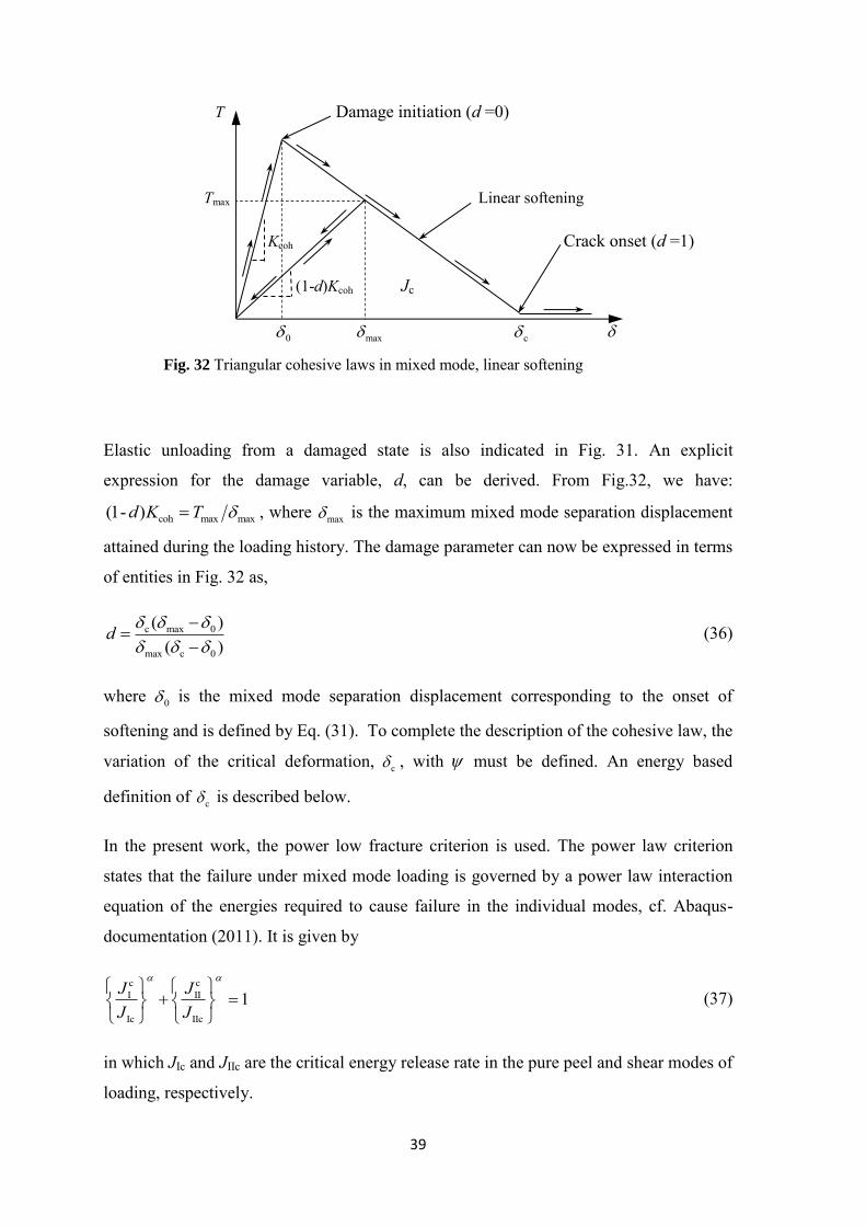
39

T Damage initiation (d =0)

Tmax Linear softening

Kcoh Crack onset (d =1)

(1-d)Kcoh Jc

0 max c Fig. 32 Triangular cohesive laws in mixed mode, linear softening

Elastic unloading from a damaged state is also indicated in Fig. 31. An explicit

expression for the damage variable, d, can be derived. From Fig.32, we have:

coh max max(1- )d K T , where max is the maximum mixed mode separation displacement

attained during the loading history. The damage parameter can now be expressed in terms

of entities in Fig. 32 as,

c max 0

max c 0

( )( )

d

(36)

where 0 is the mixed mode separation displacement corresponding to the onset of

softening and is defined by Eq. (31). To complete the description of the cohesive law, the

variation of the critical deformation, c , with must be defined. An energy based

definition of c is described below.

In the present work, the power low fracture criterion is used. The power law criterion

states that the failure under mixed mode loading is governed by a power law interaction

equation of the energies required to cause failure in the individual modes, cf. Abaqus-

documentation (2011). It is given by

c cI II

Ic IIc

1J JJ J

(37)

in which JIc and JIIc are the critical energy release rate in the pure peel and shear modes of

loading, respectively.

40

In Eq. (37), cIJ and c

IIJ refer to energy release rates in normal and shear direction,

corresponding to the fracture onset under mixed mode loading, that satisfy Eq. (37). The

critical mixed-mode energy release rate is Jc= cIJ + c

IIJ .

Equation (37) can be reformulated in the following form

1c cI c II c

cIc IIc

/ /J J J JJJ J

(38)

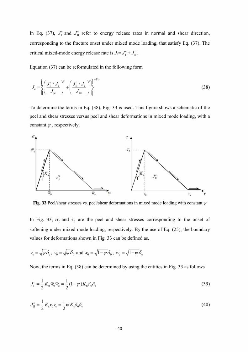
To determine the terms in Eq. (38), Fig. 33 is used. This figure shows a schematic of the

peel and shear stresses versus peel and shear deformations in mixed mode loading, with a

constant ψ , respectively.

Fig. 33 Peel/shear stresses vs. peel/shear deformations in mixed mode loading with constant ψ

In Fig. 33, 0 and 0 are the peel and shear stresses corresponding to the onset of

softening under mixed mode loading, respectively. By the use of Eq. (25), the boundary

values for deformations shown in Fig. 33 can be defined as,

c cv , 0 0v and 0 01w , c c1w

Now, the terms in Eq. (38) can be determined by using the entities in Fig. 33 as follows

cI n 0 c n 0 c

1 1 (1 )2 2

J K w w K

(39)

cII s 0 c s 0 c

1 12 2

J K v v K

(40)

41

On the other hand, for the bilinear form of T( ), Jc can also be defined as the area under

the curve shown in Fig. 32. That is equal to

c coh 0 c12

J K (41)

This result can also be obtained by adding the peel and shear fracture energies in Eqs.

(39) and (40) and use of Eq. (35). Inserting Eqs. (39), (40) and (41) into Eq. (38) gives

the final expression for the critical energy release rate as a function of loading direction,

,

1

s nc

coh IIc coh Ic

(1 )K KJK J K J

(42)

Putting equal Eqs. (41) and (42) yields the wanted expression for the critical separation

displacement in mixed mode loading as a function of loading direction variable, ,

1

s nc

coh 0 coh IIc coh Ic

(1 )2 K KK K J K J

(43)

where 0 is the mixed mode separation displacement corresponding to the onset of

softening, cf. Eq. (31) and Kcoh is the initial stiffness in mixed mode loading, cf. Eq. (35).

By introducing

s

n

K vK w

Eq. (43) can be reformulated in the following form.

12 2

ccoh 0 IIc Ic

2(1 ) 1K J J

(44)

For Kn=Ks, Eq. (44) takes the form of the corresponding equation in Camanho and Davila

(2002).

42

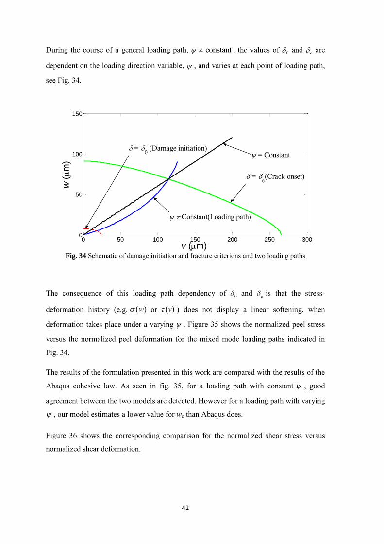
During the course of a general loading path, constant , the values of 0 and c are

dependent on the loading direction variable, , and varies at each point of loading path,

see Fig. 34.

Fig. 34 Schematic of damage initiation and fracture criterions and two loading paths

The consequence of this loading path dependency of 0 and c is that the stress-

deformation history (e.g. ( )w or ( )v ) does not display a linear softening, when

deformation takes place under a varying . Figure 35 shows the normalized peel stress

versus the normalized peel deformation for the mixed mode loading paths indicated in

Fig. 34.

The results of the formulation presented in this work are compared with the results of the

Abaqus cohesive law. As seen in fig. 35, for a loading path with constant , good

agreement between the two models are detected. However for a loading path with varying

, our model estimates a lower value for wc than Abaqus does.

Figure 36 shows the corresponding comparison for the normalized shear stress versus

normalized shear deformation.

0 50 100 150 200 250 3000

50

100

150

v (m)

w (m

)

= c(Crack onset)

Constant(Loading path)

= Constant = 0 (Damage initiation)

43

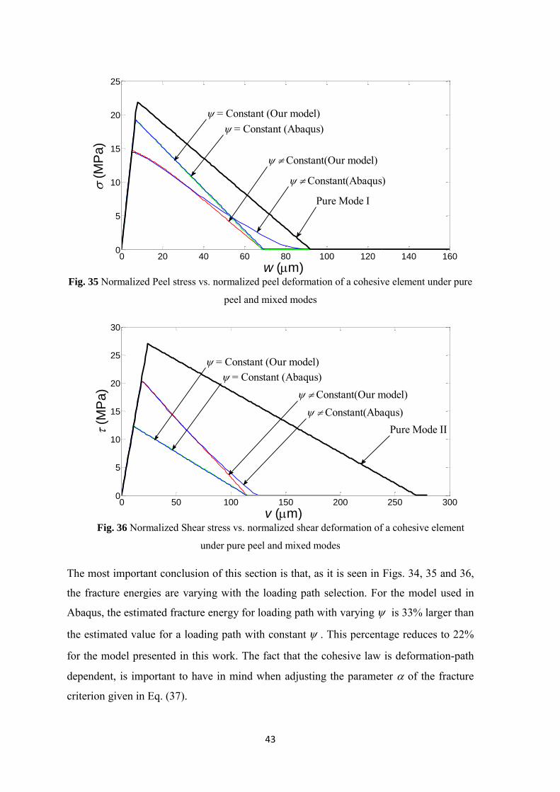
Fig. 35 Normalized Peel stress vs. normalized peel deformation of a cohesive element under pure

peel and mixed modes

Fig. 36 Normalized Shear stress vs. normalized shear deformation of a cohesive element

under pure peel and mixed modes

The most important conclusion of this section is that, as it is seen in Figs. 34, 35 and 36,

the fracture energies are varying with the loading path selection. For the model used in

Abaqus, the estimated fracture energy for loading path with varying is 33% larger than

the estimated value for a loading path with constant . This percentage reduces to 22%

for the model presented in this work. The fact that the cohesive law is deformation-path

dependent, is important to have in mind when adjusting the parameter of the fracture

criterion given in Eq. (37).

0 20 40 60 80 100 120 140 1600

5

10

15

20

25

w (m)

(

MP

a)

= Constant (Our model)

Constant(Abaqus)

Constant(Our model)

Pure Mode I

= Constant (Abaqus)

0 50 100 150 200 250 3000

5

10

15

20

25

30

(M

Pa)

v (m)

= Constant (Our model) = Constant (Abaqus)

Constant(Abaqus) Constant(Our model)

Pure Mode II

44

3 Experiments

In this chapter, DCB- and ENF-tests are evaluated and used to obtain the cohesive laws’

parameters for modes I and II of loading for an adhesive layer. These parameters along

with the results of the MCB-tests are used in the next chapter to find the best estimation

of α, the power coefficient in the damage evolution criterion in Eq. (37). Subsequently by

use of all the obtained parameters, the TRB-tests are simulated and the results are verified

with the experimental results of TRB-tests, carried out in the last part of this chapter. The

four setups of specimens used in this work are summarized in Table 1. The material

properties of the specimens are given in Table 2. The adhesive used in this work is an

epoxy considered for reinforcing of bridges, cf. Tab. 2.

Table 1. Specimen type, number and the objective of study

Type of Specimen No. of

Specimen

Objective

DCB

3

Determination

of cohesive law

ENF

3 Determination of

cohesive law

MCB

6 Determination

of α

TRB

16 P–Δ curves

45

Table 2. Material properties of specimens

Material E (GPa) σy (MPa)

Adhesivea 7b 0.3 20

Steel (Rigor) 196c 0.29 500

Aluminum 63c 0.31 276 a Sto BPE Lim567 b Information provided by the manufacturer c Information provided by the experiments

3.1 DCB-experiments

Experiments have been carried out using a set of DCB-specimens to determine the

cohesive laws’ parameters for mode I of loading, cf. André et al. (2012). These results are

repeated here for completeness. The geometry of the specimens is given in Fig. 10. The

dimensions are: h = 6.6 mm, t = 2.4 mm, a = 80 mm, b = 8.3 mm and l = 200 mm.

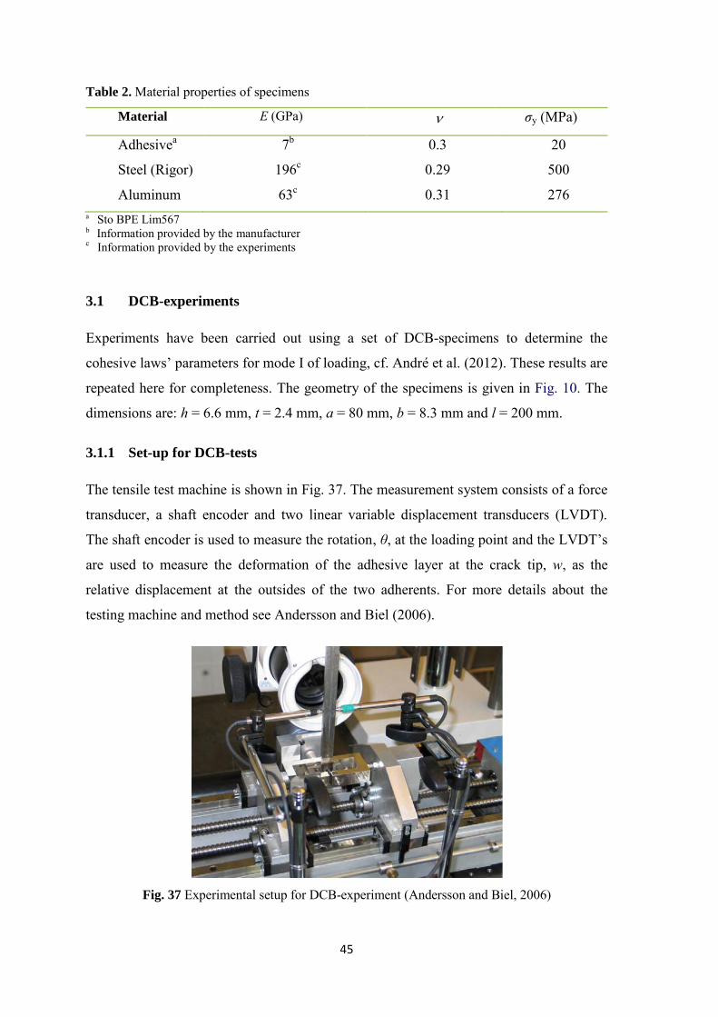
3.1.1 Set-up for DCB-tests

The tensile test machine is shown in Fig. 37. The measurement system consists of a force

transducer, a shaft encoder and two linear variable displacement transducers (LVDT).

The shaft encoder is used to measure the rotation, θ, at the loading point and the LVDT’s

are used to measure the deformation of the adhesive layer at the crack tip, w, as the

relative displacement at the outsides of the two adherents. For more details about the

testing machine and method see Andersson and Biel (2006).

Fig. 37 Experimental setup for DCB-experiment (Andersson and Biel, 2006)

46

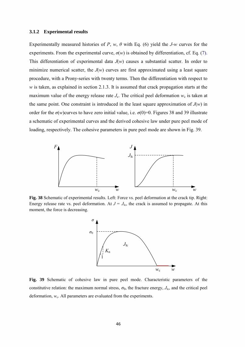
3.1.2 Experimental results

Experimentally measured histories of P, w, θ with Eq. (6) yield the J-w curves for the

experiments. From the experimental curve, σ(w) is obtained by differentiation, cf. Eq. (7).

This differentiation of experimental data J(w) causes a substantial scatter. In order to

minimize numerical scatter, the J(w) curves are first approximated using a least square

procedure, with a Prony-series with twenty terms. Then the differentiation with respect to

w is taken, as explained in section 2.1.3. It is assumed that crack propagation starts at the

maximum value of the energy release rate Jc. The critical peel deformation wc is taken at

the same point. One constraint is introduced in the least square approximation of J(w) in

order for the σ(w)curves to have zero initial value, i.e. σ(0)=0. Figures 38 and 39 illustrate

a schematic of experimental curves and the derived cohesive law under pure peel mode of

loading, respectively. The cohesive parameters in pure peel mode are shown in Fig. 39.

F J

JIc

wc w wc w

Fig. 38 Schematic of experimental results. Left: Force vs. peel deformation at the crack tip. Right: Energy release rate vs. peel deformation. At J = JIc, the crack is assumed to propagate. At this moment, the force is decreasing.

σ σ0

JIc Kn 1 wc w

Fig. 39 Schematic of cohesive law in pure peel mode. Characteristic parameters of the

constitutive relation: the maximum normal stress, σ0, the fracture energy, JIc, and the critical peel

deformation, wc. All parameters are evaluated from the experiments.

47

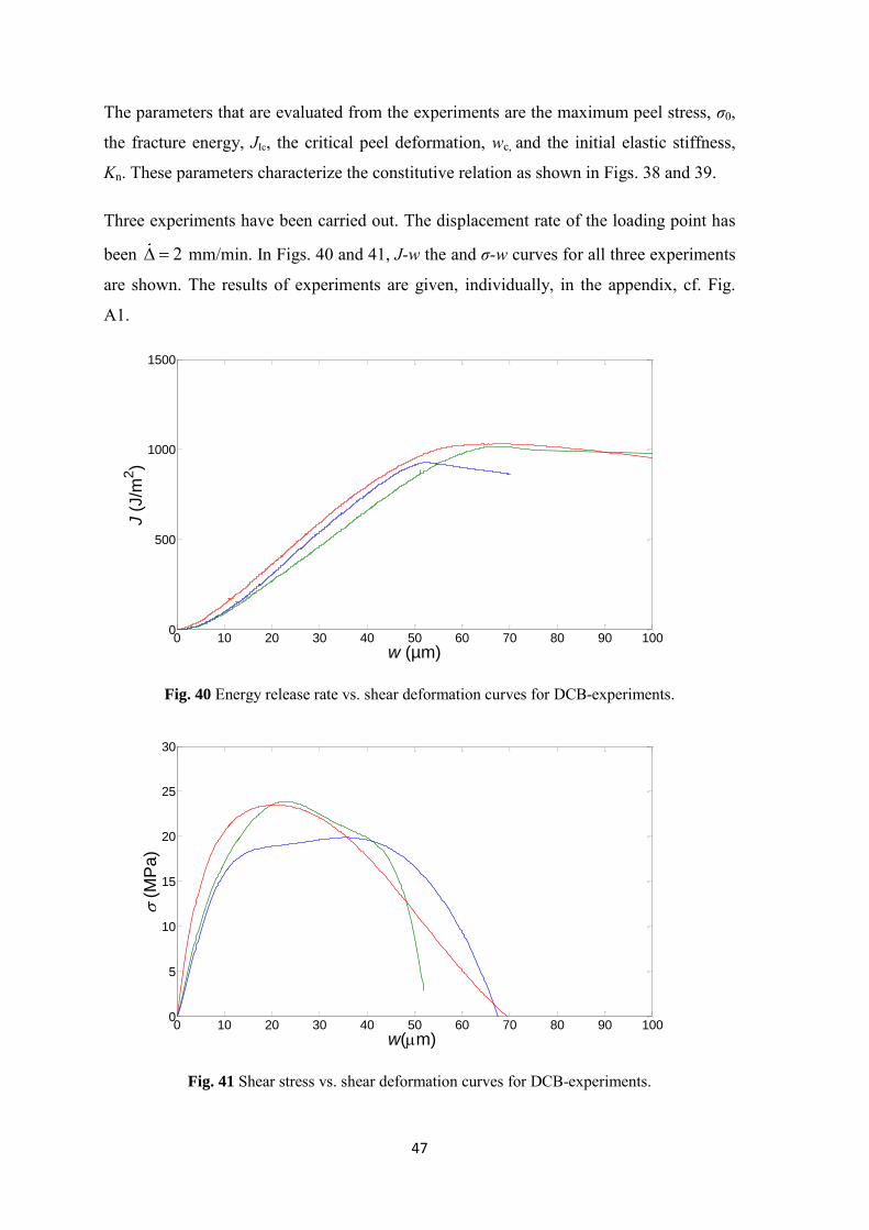
The parameters that are evaluated from the experiments are the maximum peel stress, σ0,

the fracture energy, JIc, the critical peel deformation, wc, and the initial elastic stiffness,

Kn. These parameters characterize the constitutive relation as shown in Figs. 38 and 39.

Three experiments have been carried out. The displacement rate of the loading point has

been 2 mm/min. In Figs. 40 and 41, J-w the and σ-w curves for all three experiments

are shown. The results of experiments are given, individually, in the appendix, cf. Fig.

A1.

Fig. 40 Energy release rate vs. shear deformation curves for DCB-experiments.

Fig. 41 Shear stress vs. shear deformation curves for DCB-experiments.

0 10 20 30 40 50 60 70 80 90 1000

500

1000

1500

w (µm)

J (

J/m

2)

0 10 20 30 40 50 60 70 80 90 1000

5

10

15

20

25

30

w(m)

(

MP

a)

48

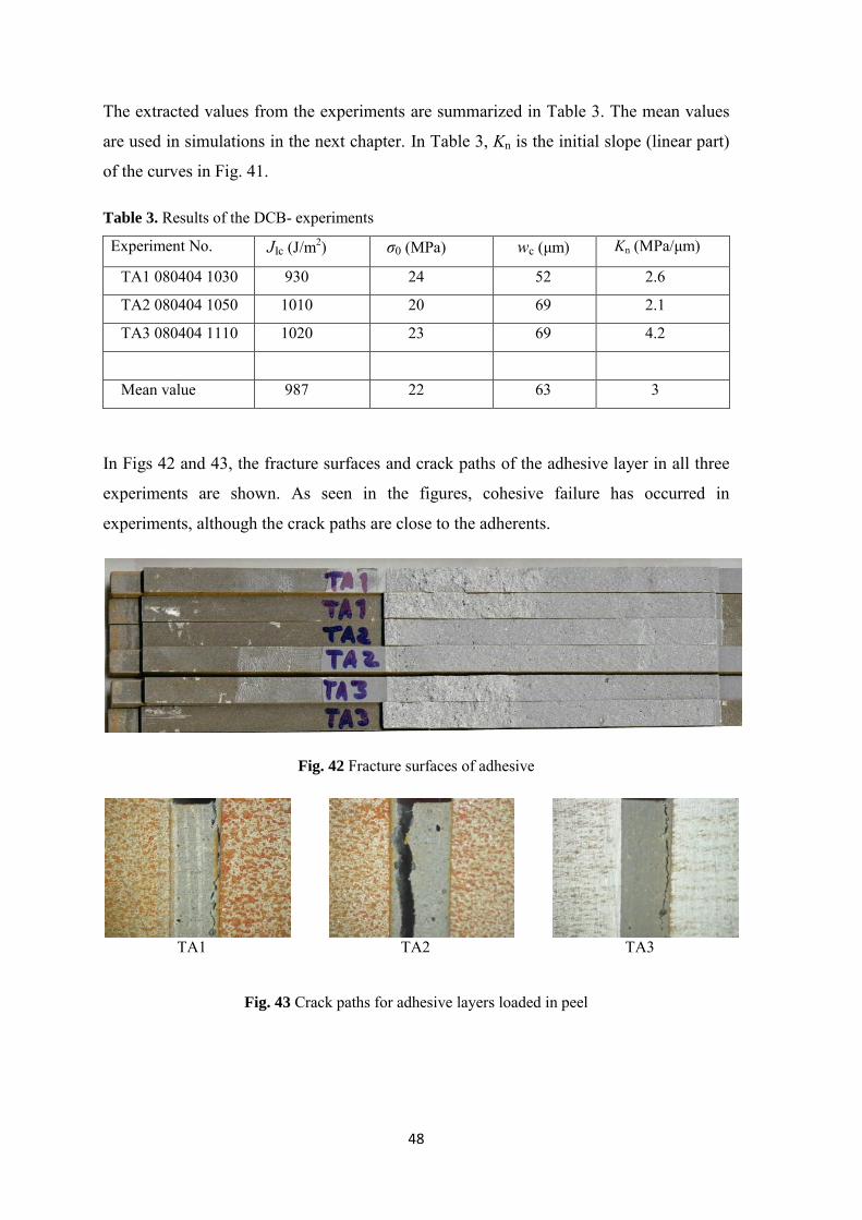
The extracted values from the experiments are summarized in Table 3. The mean values

are used in simulations in the next chapter. In Table 3, Kn is the initial slope (linear part)

of the curves in Fig. 41.

Table 3. Results of the DCB- experiments

Experiment No. JIc (J/m2) σ0 (MPa) wc (μm) Kn (MPa/μm)

TA1 080404 1030 930 24 52 2.6

TA2 080404 1050 1010 20 69 2.1

TA3 080404 1110 1020 23 69 4.2

Mean value 987 22 63 3

In Figs 42 and 43, the fracture surfaces and crack paths of the adhesive layer in all three

experiments are shown. As seen in the figures, cohesive failure has occurred in

experiments, although the crack paths are close to the adherents.

Fig. 42 Fracture surfaces of adhesive

TA1

TA2

TA3

Fig. 43 Crack paths for adhesive layers loaded in peel

49

3.2 ENF-experiments

Experiments are carried out using a set of ENF-specimens to determine the strength and

fracture energy for mode II of loading. The geometry of the specimens is given in Fig. 12.

The dimensions of specimens are: h = 16.6 mm, t = 2.4 mm, a = 350 mm, b = 16.6 mm

and l = 1000 mm, where the out-of-plane width of the specimen is denoted b.

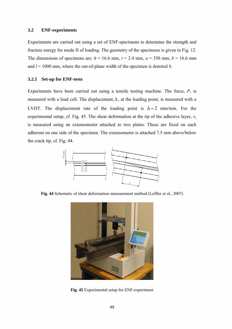
3.2.1 Set-up for ENF-tests

Experiments have been carried out using a tensile testing machine. The force, P, is

measured with a load cell. The displacement, , at the loading point, is measured with a

LVDT. The displacement rate of the loading point is 2 mm/min. For the

experimental setup, cf. Fig. 45. The shear deformation at the tip of the adhesive layer, v,

is measured using an extensometer attached to two plates. These are fixed on each

adherent on one side of the specimen. The extensometer is attached 7.5 mm above/below

the crack tip, cf. Fig. 44.

Fig. 44 Schematic of shear deformation measurement method (Leffler et al., 2007)

Fig. 45 Experimental setup for ENF-experiment

50

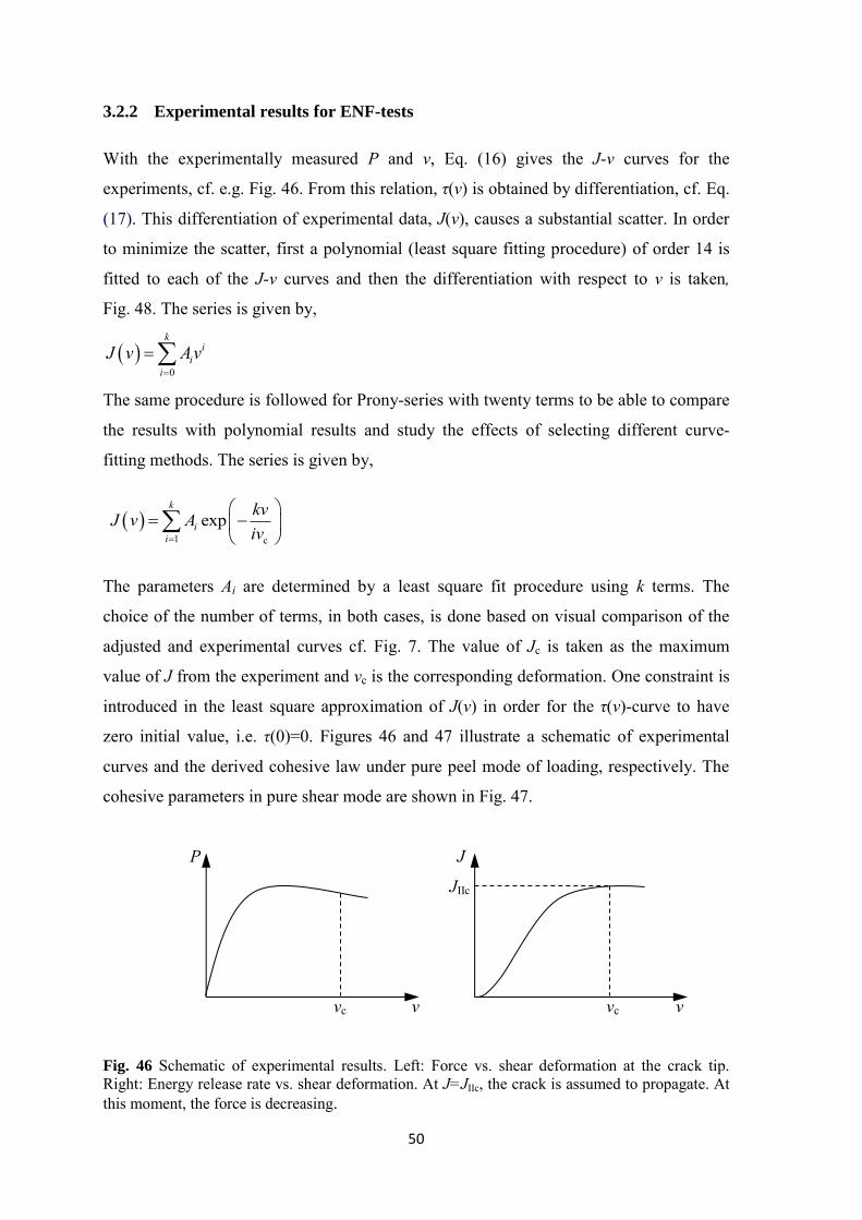
3.2.2 Experimental results for ENF-tests

With the experimentally measured P and v, Eq. (16) gives the J-v curves for the

experiments, cf. e.g. Fig. 46. From this relation, τ(v) is obtained by differentiation, cf. Eq.

(17). This differentiation of experimental data, J(v), causes a substantial scatter. In order

to minimize the scatter, first a polynomial (least square fitting procedure) of order 14 is

fitted to each of the J-v curves and then the differentiation with respect to v is taken,

Fig. 48. The series is given by,

0

ki

ii

J v Av

The same procedure is followed for Prony-series with twenty terms to be able to compare

the results with polynomial results and study the effects of selecting different curve-

fitting methods. The series is given by,

1 c

expk

ii

kvJ v Aiv

The parameters Ai are determined by a least square fit procedure using k terms. The

choice of the number of terms, in both cases, is done based on visual comparison of the

adjusted and experimental curves cf. Fig. 7. The value of Jc is taken as the maximum

value of J from the experiment and vc is the corresponding deformation. One constraint is

introduced in the least square approximation of J(v) in order for the τ(v)-curve to have

zero initial value, i.e. τ(0)=0. Figures 46 and 47 illustrate a schematic of experimental

curves and the derived cohesive law under pure peel mode of loading, respectively. The

cohesive parameters in pure shear mode are shown in Fig. 47.

P J

JIIc

vc v vc v

Fig. 46 Schematic of experimental results. Left: Force vs. shear deformation at the crack tip. Right: Energy release rate vs. shear deformation. At J=JIIc, the crack is assumed to propagate. At this moment, the force is decreasing.

51

τ τ0

JIIc Ks 1 vc v

Fig. 47 Schematic of cohesive law in pure shear mode. Characteristic parameters of the constitutive relation: the maximum shear stress, τ0, the fracture energy, JIIc, and the critical shear deformation, vc. All parameters are evaluated from the experiments. The parameters that are extracted from the experiments are the maximum shear stress, τ0,

the fracture energy, JIIc, and the critical shear deformation, vc. These parameters

characterize the constitutive relation shown in Figs. 46 and 47.

Three experiments have been carried out. In Fig. 48, the J-v curves for all three

experiments fitted with the Prony series curves are shown and subsequently the τ-v curves

are derived and shown in Fig. 49. The results of experiments are given, individually, in

the appendix, cf. Fig. A2.

Fig. 48 Experimental results and fitted Prony series curves for ENF-experiments.

0 50 100 150 200 250 300 3500

500

1000

1500

2000

2500

3000

3500

4000

4500

5000

(m)

J (

J/m

2)

Experiment 1

Experiment 2Experiment 3

52

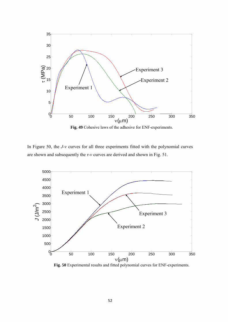
Fig. 49 Cohesive laws of the adhesive for ENF-experiments.

In Figure 50, the J-v curves for all three experiments fitted with the polynomial curves

are shown and subsequently the τ-v curves are derived and shown in Fig. 51.

Fig. 50 Experimental results and fitted polynomial curves for ENF-experiments.

0 50 100 150 200 250 300 3500

5

10

15

20

25

30

35

(m)

(M

Pa

)

Experiment 1Experiment 2

Experiment 3

0 50 100 150 200 250 300 3500

500

1000

1500

2000

2500

3000

3500

4000

4500

5000

(m)

J (

J/m

2)

Experiment 1

Experiment 2

Experiment 3

53

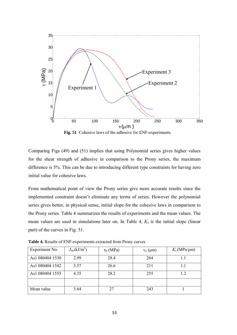
Fig. 51 Cohesive laws of the adhesive for ENF-experiments.

Comparing Figs (49) and (51) implies that using Polynomial series gives higher values

for the shear strength of adhesive in comparison to the Prony series, the maximum

difference is 5%. This can be due to introducing different type constraints for having zero

initial value for cohesive laws.

From mathematical point of view the Prony series give more accurate results since the

implemented constraint doesn’t eliminate any terms of series. However the polynomial

series gives better, in physical sense, initial slope for the cohesive laws in comparison to

the Prony series. Table 4 summarizes the results of experiments and the mean values. The

mean values are used in simulations later on. In Table 4, Ks is the initial slope (linear

part) of the curves in Fig. 51.

Table 4. Results of ENF-experiments extracted from Prony curves

Experiment No. JIIc(kJ/m2) τ0 (MPa) vc (μm) Ks (MPa/μm)

As1 080404 1530 2.99 28.4 264 1.1

As1 080404 1542 3.57 26.6 211 1.1

As1 080404 1555 4.35 28.2 255 1.2

Mean value 3.64 27 243 1

0 50 100 150 200 250 300 3500

5

10

15

20

25

30

35

(m )

(M

Pa

)

Experiment 1

Experiment 3

Experiment 2

54

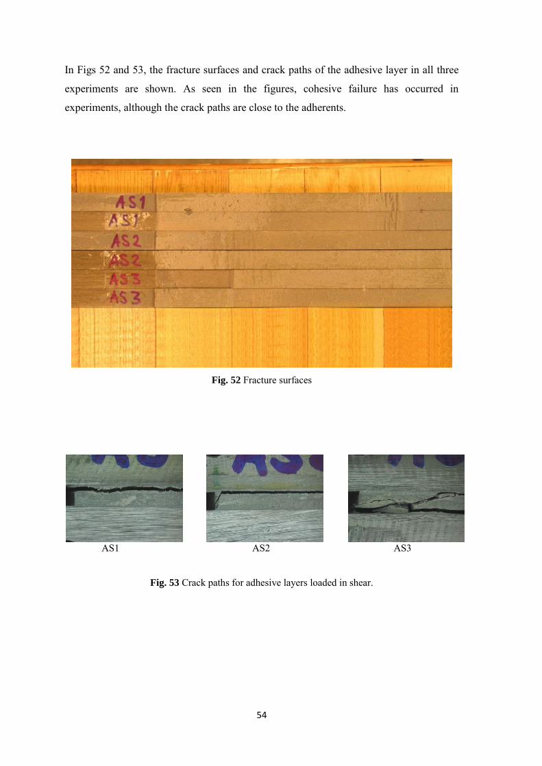
In Figs 52 and 53, the fracture surfaces and crack paths of the adhesive layer in all three

experiments are shown. As seen in the figures, cohesive failure has occurred in

experiments, although the crack paths are close to the adherents.

Fig. 52 Fracture surfaces

AS1

AS2

AS3

Fig. 53 Crack paths for adhesive layers loaded in shear.

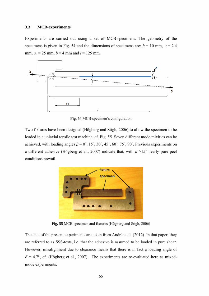
55

3.3 MCB-experiments

Experiments are carried out using a set of MCB-specimens. The geometry of the

specimens is given in Fig. 54 and the dimensions of specimens are: h = 10 mm, t = 2.4

mm, a0 = 25 mm, b = 4 mm and l = 125 mm.

Fig. 54 MCB-specimen’s configuration

Two fixtures have been designed (Högberg and Stigh, 2006) to allow the specimen to be

loaded in a uniaxial tensile test machine, cf. Fig. 55. Seven different mode mixities can be

achieved, with loading angles β = 0˚, 15˚, 30˚, 45˚, 60˚, 75˚, 90˚. Previous experiments on

a different adhesive (Högberg et al., 2007) indicate that, with β ≥15˚ nearly pure peel

conditions prevail.

Fig. 55 MCB-specimen and fixtures (Högberg and Stigh, 2006)

The data of the present experiments are taken from André et al. (2012). In that paper, they

are referred to as SSS-tests, i.e. that the adhesive is assumed to be loaded in pure shear.

However, misalignment due to clearance means that there is in fact a loading angle of

= 4.7, cf. (Högberg et al., 2007). The experiments are re-evaluated here as mixed-

mode experiments.

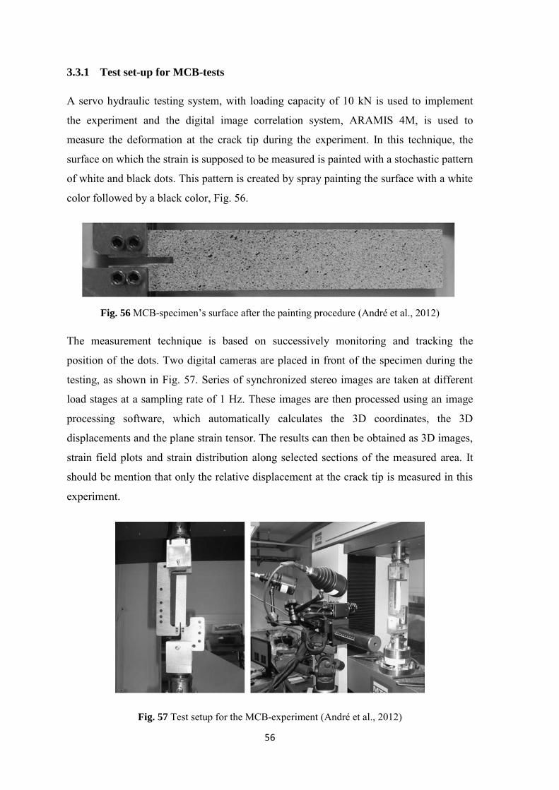
56

3.3.1 Test set-up for MCB-tests

A servo hydraulic testing system, with loading capacity of 10 kN is used to implement

the experiment and the digital image correlation system, ARAMIS 4M, is used to

measure the deformation at the crack tip during the experiment. In this technique, the

surface on which the strain is supposed to be measured is painted with a stochastic pattern

of white and black dots. This pattern is created by spray painting the surface with a white

color followed by a black color, Fig. 56.

Fig. 56 MCB-specimen’s surface after the painting procedure (André et al., 2012)

The measurement technique is based on successively monitoring and tracking the

position of the dots. Two digital cameras are placed in front of the specimen during the

testing, as shown in Fig. 57. Series of synchronized stereo images are taken at different

load stages at a sampling rate of 1 Hz. These images are then processed using an image

processing software, which automatically calculates the 3D coordinates, the 3D

displacements and the plane strain tensor. The results can then be obtained as 3D images,

strain field plots and strain distribution along selected sections of the measured area. It

should be mention that only the relative displacement at the crack tip is measured in this

experiment.

Fig. 57 Test setup for the MCB-experiment (André et al., 2012)

57

3.3.2 Experimental results for MCB-tests

The ARAMIS 4M system records the displacements in the crack tip area. The

displacements of four particular points at the crack tip, cf. Fig. 58, are extracted from the

system for determination of the rotation of the adherents and the shear and peel

deformation of the adhesive layer to be calculated, cf. Fig. 59. The positions are

measured in both x and y directions. The rotations of the adherents at the crack tip are

evaluated by

x,1 x,2u

1 2

u uy y

,

x,3 x,4l

3 4

u uy y

The shear deformation of the adhesive becomes:

x,2 x,3 m y,3 y,2v u u u u

and the peel deformation is given by

y,2 y,3 m x,3 x,2w u u u u

where u lm 2

is the mean value of the rotation angles of adherents, cf. Högberg

et al. (2007).

Fig. 58 Position of the points used to define the rotation angles of adherents

58

Fig. 59 Experimental rotation angles of the adherents for Experiment 4

Six experiments are carried out. Figure 60 shows the S-δ curves for the experiments

where δ is the separation displacement at the crack tip. With the experimentally measured

S, v, w, θ1 and θ2, Eq. (21) gives the J-δ curves shown in Fig. 61. Figure 62 shows the

peel vs. shear deformations at the crack tip, measured durring the experiment. The results

of experiments are given, individually, in the appendix, cf. Fig. A3.

Fig. 60 Experimental results of MCB-tests. Force vs. displacement at the crack tip.

0 50 100 150 200 250 300 350 400 450 500-3

-2.5

-2

-1.5

-1

-0.5

0

(µm)

(

de

g)

Lower adherent

Upper adherent

0 50 100 150 200 250 3000

500

1000

1500

2000

2500

3000

3500

4000

4500

(µm)

S (

N)

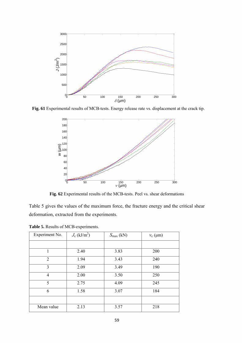
59

Fig. 61 Experimental results of MCB-tests. Energy release rate vs. displacement at the crack tip.

Fig. 62 Experimental results of the MCB-tests. Peel vs. shear deformations

Table 5 gives the values of the maximum force, the fracture energy and the critical shear

deformation, extracted from the experiments.

Table 5. Results of MCB-experiments.

Experiment No. Jc (kJ/m2) Smax (kN) vc (μm)

1 2.40 3.83 200

2 1.94 3.43 240

3 2.09 3.49 190

4 2.00 3.50 250

5 2.75 4.09 245

6 1.58 3.07 184

Mean value 2.13 3.57 218

0 50 100 150 200 250 3000

500

1000

1500

2000

2500

3000

(µm)

J (

J/m

2)

0 50 100 150 200 250 3000

20

40

60

80

100

120

140

160

180

200

(µm)

w (

µm

)

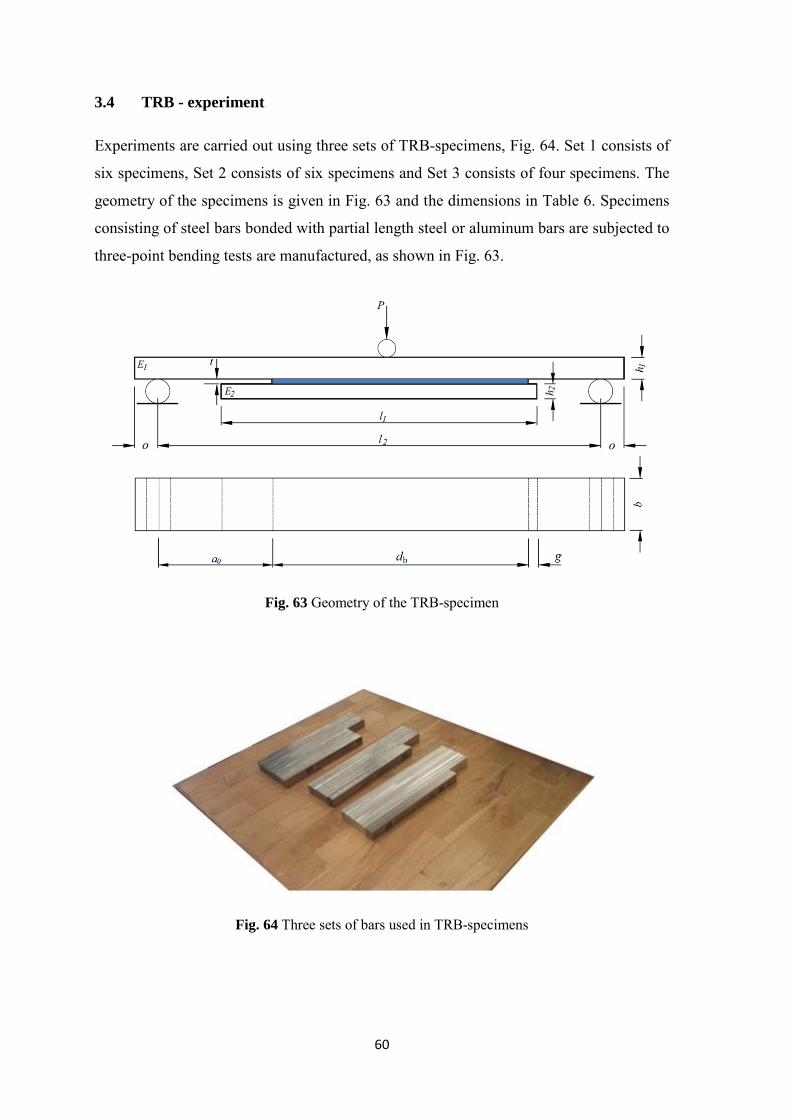
60

3.4 TRB - experiment

Experiments are carried out using three sets of TRB-specimens, Fig. 64. Set 1 consists of

six specimens, Set 2 consists of six specimens and Set 3 consists of four specimens. The

geometry of the specimens is given in Fig. 63 and the dimensions in Table 6. Specimens

consisting of steel bars bonded with partial length steel or aluminum bars are subjected to

three-point bending tests are manufactured, as shown in Fig. 63.

Fig. 63 Geometry of the TRB-specimen

Fig. 64 Three sets of bars used in TRB-specimens

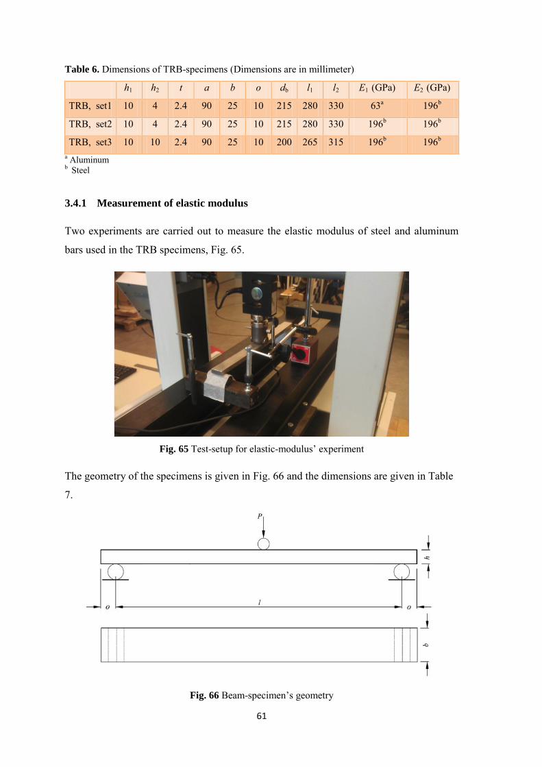
61

Table 6. Dimensions of TRB-specimens (Dimensions are in millimeter)

h1 h2 t a b o db l1 l2 E1 (GPa) E2 (GPa)

TRB, set1 10 4 2.4 90 25 10 215 280 330 63a 196b

TRB, set2 10 4 2.4 90 25 10 215 280 330 196b 196b

TRB, set3 10 10 2.4 90 25 10 200 265 315 196b 196b a Aluminum b Steel 3.4.1 Measurement of elastic modulus

Two experiments are carried out to measure the elastic modulus of steel and aluminum

bars used in the TRB specimens, Fig. 65.

Fig. 65 Test-setup for elastic-modulus’ experiment

The geometry of the specimens is given in Fig. 66 and the dimensions are given in Table

7.

Fig. 66 Beam-specimen’s geometry

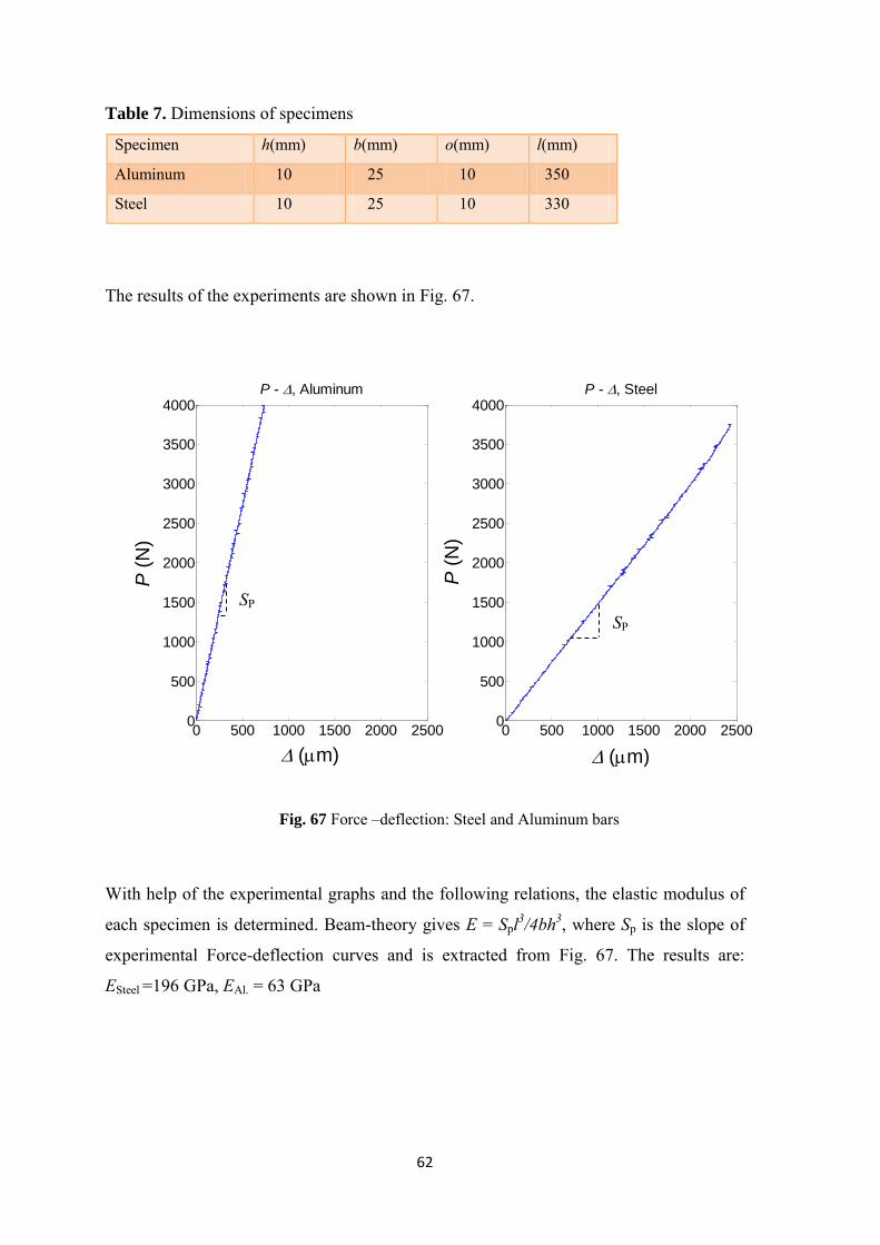
62

Table 7. Dimensions of specimens

Specimen h(mm) b(mm) o(mm) l(mm)

Aluminum 10 25 10 350

Steel 10 25 10 330

The results of the experiments are shown in Fig. 67.

Fig. 67 Force –deflection: Steel and Aluminum bars

With help of the experimental graphs and the following relations, the elastic modulus of

each specimen is determined. Beam-theory gives E = Spl3/4bh3, where Sp is the slope of

experimental Force-deflection curves and is extracted from Fig. 67. The results are:

ESteel =196 GPa, EAl. = 63 GPa

0 500 1000 1500 2000 25000

500

1000

1500

2000

2500

3000

3500

4000P - , Aluminum

(m)

P (

N)

0 500 1000 1500 2000 25000

500

1000

1500

2000

2500

3000

3500

4000P - , Steel

(m)

P (

N)

SP SP

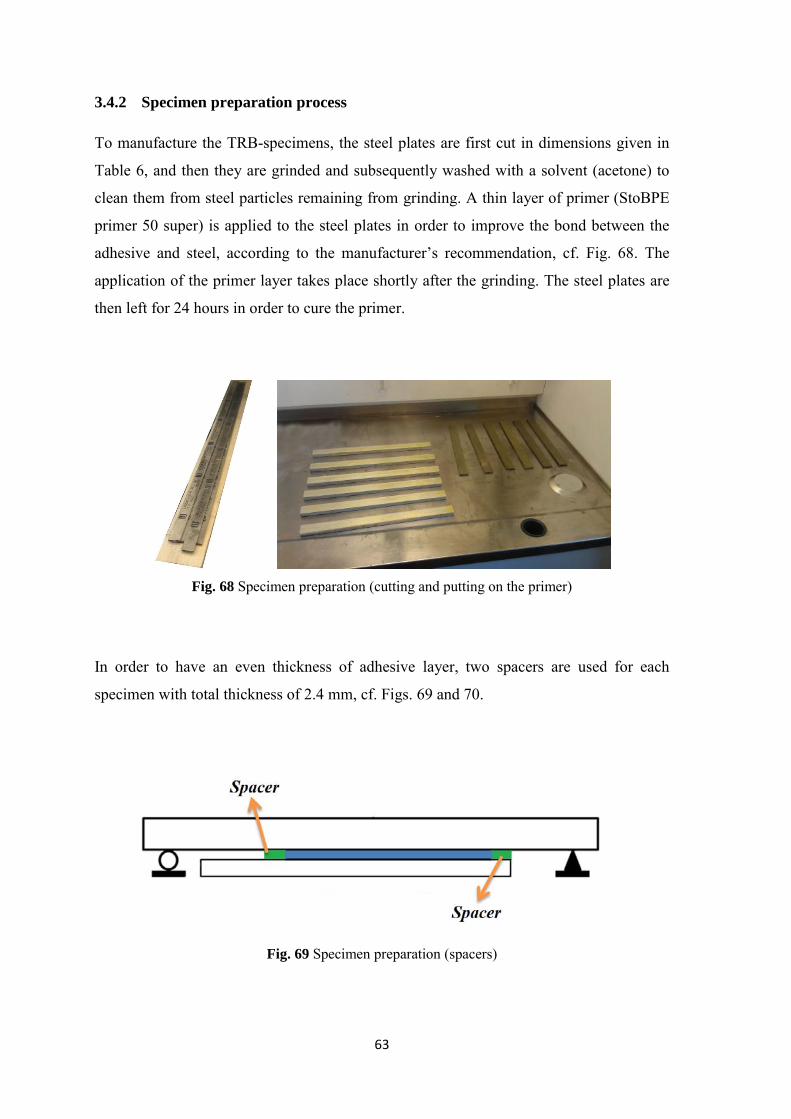
63

3.4.2 Specimen preparation process

To manufacture the TRB-specimens, the steel plates are first cut in dimensions given in

Table 6, and then they are grinded and subsequently washed with a solvent (acetone) to

clean them from steel particles remaining from grinding. A thin layer of primer (StoBPE

primer 50 super) is applied to the steel plates in order to improve the bond between the

adhesive and steel, according to the manufacturer’s recommendation, cf. Fig. 68. The

application of the primer layer takes place shortly after the grinding. The steel plates are

then left for 24 hours in order to cure the primer.

Fig. 68 Specimen preparation (cutting and putting on the primer)

In order to have an even thickness of adhesive layer, two spacers are used for each

specimen with total thickness of 2.4 mm, cf. Figs. 69 and 70.

Fig. 69 Specimen preparation (spacers)

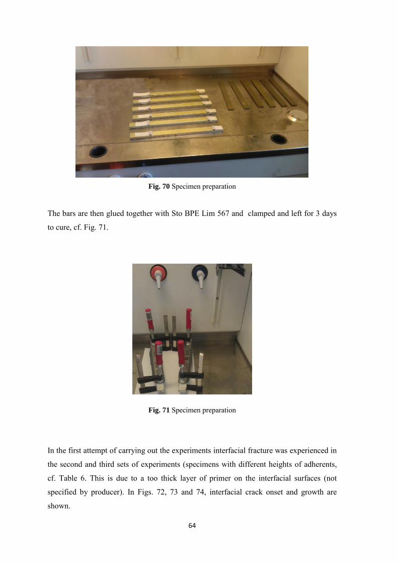
64

Fig. 70 Specimen preparation

The bars are then glued together with Sto BPE Lim 567 and clamped and left for 3 days

to cure, cf. Fig. 71.

Fig. 71 Specimen preparation

In the first attempt of carrying out the experiments interfacial fracture was experienced in

the second and third sets of experiments (specimens with different heights of adherents,

cf. Table 6. This is due to a too thick layer of primer on the interfacial surfaces (not

specified by producer). In Figs. 72, 73 and 74, interfacial crack onset and growth are

shown.

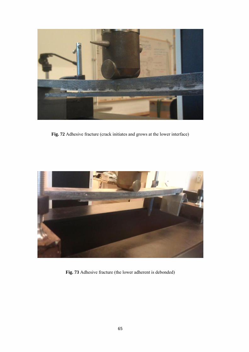
65

Fig. 72 Adhesive fracture (crack initiates and grows at the lower interface)

Fig. 73 Adhesive fracture (the lower adherent is debonded)

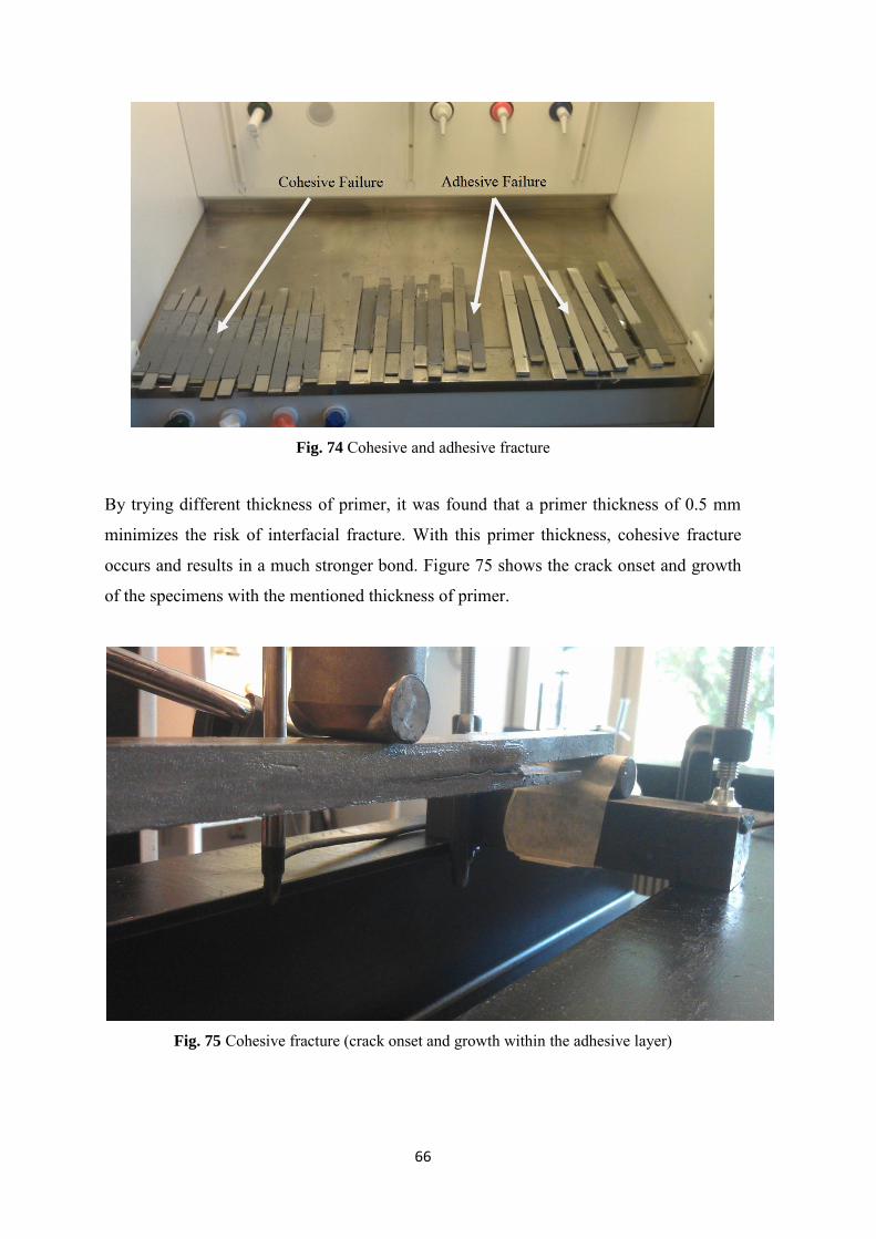
66

Fig. 74 Cohesive and adhesive fracture

By trying different thickness of primer, it was found that a primer thickness of 0.5 mm

minimizes the risk of interfacial fracture. With this primer thickness, cohesive fracture

occurs and results in a much stronger bond. Figure 75 shows the crack onset and growth

of the specimens with the mentioned thickness of primer.

Fig. 75 Cohesive fracture (crack onset and growth within the adhesive layer)

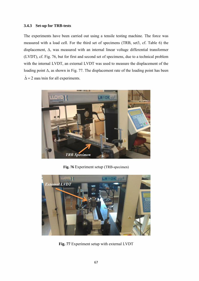
67

3.4.3 Set-up for TRB-tests

The experiments have been carried out using a tensile testing machine. The force was

measured with a load cell. For the third set of specimens (TRB, set3, cf. Table 6) the

displacement, Δ, was measured with an internal linear voltage differential transformer

(LVDT), cf. Fig. 76, but for first and second set of specimens, due to a technical problem

with the internal LVDT, an external LVDT was used to measure the displacement of the

loading point Δ, as shown in Fig. 77. The displacement rate of the loading point has been

2 mm /min for all experiments.

Fig. 76 Experiment setup (TRB-specimen)

Fig. 77 Experiment setup with external LVDT

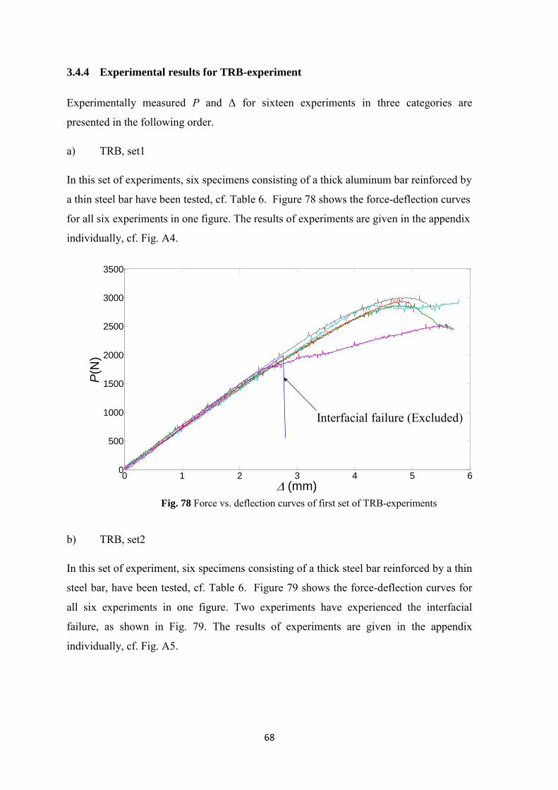
68

3.4.4 Experimental results for TRB-experiment

Experimentally measured P and Δ for sixteen experiments in three categories are

presented in the following order.

a) TRB, set1

In this set of experiments, six specimens consisting of a thick aluminum bar reinforced by

a thin steel bar have been tested, cf. Table 6. Figure 78 shows the force-deflection curves

for all six experiments in one figure. The results of experiments are given in the appendix

individually, cf. Fig. A4.

Fig. 78 Force vs. deflection curves of first set of TRB-experiments

b) TRB, set2

In this set of experiment, six specimens consisting of a thick steel bar reinforced by a thin

steel bar, have been tested, cf. Table 6. Figure 79 shows the force-deflection curves for

all six experiments in one figure. Two experiments have experienced the interfacial

failure, as shown in Fig. 79. The results of experiments are given in the appendix

individually, cf. Fig. A5.

0 1 2 3 4 5 60

500

1000

1500

2000

2500

3000

3500

(mm)

P(N

)

Interfacial failure (Excluded)

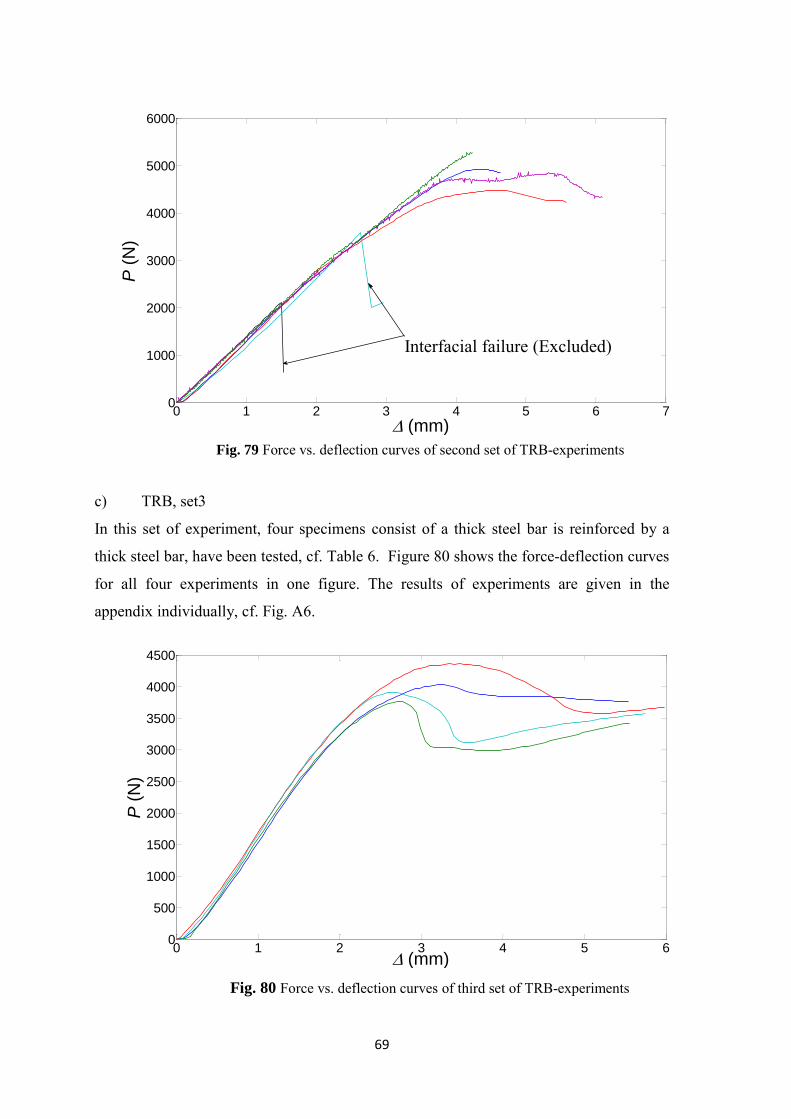
69

Fig. 79 Force vs. deflection curves of second set of TRB-experiments

c) TRB, set3

In this set of experiment, four specimens consist of a thick steel bar is reinforced by a

thick steel bar, have been tested, cf. Table 6. Figure 80 shows the force-deflection curves

for all four experiments in one figure. The results of experiments are given in the

appendix individually, cf. Fig. A6.

Fig. 80 Force vs. deflection curves of third set of TRB-experiments

0 1 2 3 4 5 6 70

1000

2000

3000

4000

5000

6000

(mm)

P (

N)

Interfacial failure (Excluded)

0 1 2 3 4 5 60

500

1000

1500

2000

2500

3000

3500

4000

4500

(mm)

P (

N)

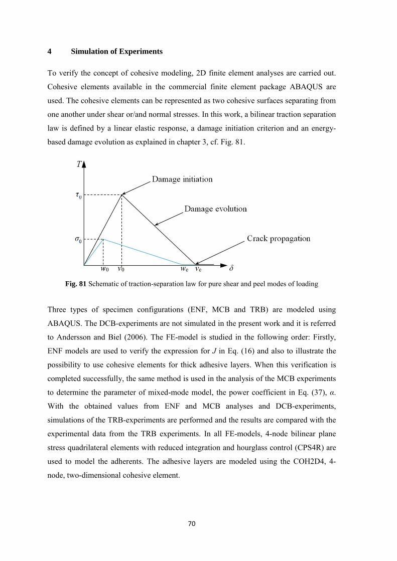
70

4 Simulation of Experiments

To verify the concept of cohesive modeling, 2D finite element analyses are carried out.

Cohesive elements available in the commercial finite element package ABAQUS are

used. The cohesive elements can be represented as two cohesive surfaces separating from

one another under shear or/and normal stresses. In this work, a bilinear traction separation

law is defined by a linear elastic response, a damage initiation criterion and an energy-

based damage evolution as explained in chapter 3, cf. Fig. 81.

Fig. 81 Schematic of traction-separation law for pure shear and peel modes of loading

Three types of specimen configurations (ENF, MCB and TRB) are modeled using

ABAQUS. The DCB-experiments are not simulated in the present work and it is referred

to Andersson and Biel (2006). The FE-model is studied in the following order: Firstly,

ENF models are used to verify the expression for J in Eq. (16) and also to illustrate the

possibility to use cohesive elements for thick adhesive layers. When this verification is

completed successfully, the same method is used in the analysis of the MCB experiments

to determine the parameter of mixed-mode model, the power coefficient in Eq. (37), α.

With the obtained values from ENF and MCB analyses and DCB-experiments,

simulations of the TRB-experiments are performed and the results are compared with the

experimental data from the TRB experiments. In all FE-models, 4-node bilinear plane

stress quadrilateral elements with reduced integration and hourglass control (CPS4R) are

used to model the adherents. The adhesive layers are modeled using the COH2D4, 4-

node, two-dimensional cohesive element.

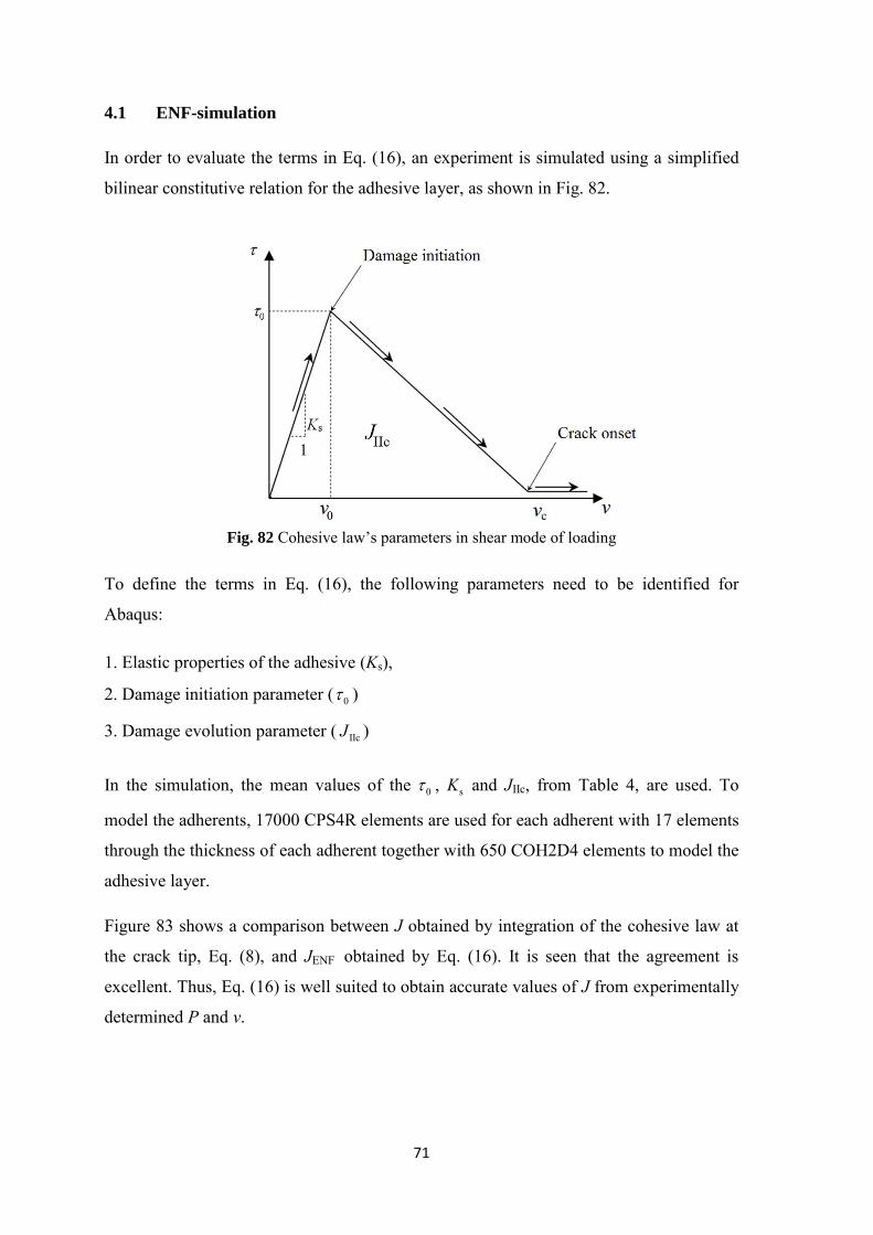
71

4.1 ENF-simulation

In order to evaluate the terms in Eq. (16), an experiment is simulated using a simplified

bilinear constitutive relation for the adhesive layer, as shown in Fig. 82.

1

Fig. 82 Cohesive law’s parameters in shear mode of loading

To define the terms in Eq. (16), the following parameters need to be identified for

Abaqus:

1. Elastic properties of the adhesive (Ks),

2. Damage initiation parameter ( 0 )

3. Damage evolution parameter ( IIcJ )

In the simulation, the mean values of the 0 , sK and JIIc, from Table 4, are used. To

model the adherents, 17000 CPS4R elements are used for each adherent with 17 elements

through the thickness of each adherent together with 650 COH2D4 elements to model the

adhesive layer.

Figure 83 shows a comparison between J obtained by integration of the cohesive law at

the crack tip, Eq. (8), and JENF obtained by Eq. (16). It is seen that the agreement is

excellent. Thus, Eq. (16) is well suited to obtain accurate values of J from experimentally

determined P and v.

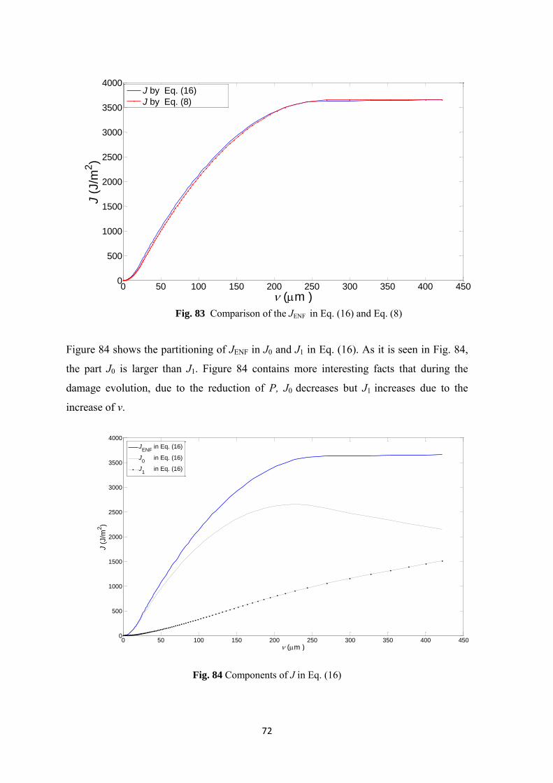
72

Fig. 83 Comparison of the JENF in Eq. (16) and Eq. (8)

Figure 84 shows the partitioning of JENF in J0 and J1 in Eq. (16). As it is seen in Fig. 84,

the part J0 is larger than J1. Figure 84 contains more interesting facts that during the

damage evolution, due to the reduction of P, J0 decreases but J1 increases due to the

increase of v.

Fig. 84 Components of J in Eq. (16)

0 50 100 150 200 250 300 350 400 4500

500

1000

1500

2000

2500

3000

3500

4000

(m )

J (

J/m

2)

J by Eq. (16)

J by Eq. (8)

0 50 100 150 200 250 300 350 400 4500

500

1000

1500

2000

2500

3000

3500

4000

(m )

J (

J/m

2)

JENF

in Eq. (16)

J0 in Eq. (16)

J1 in Eq. (16)

73

Figure 85 shows good agreement between the experimental J-v curves and the result of

ENF-simulation.

Fig. 85 Energy release rate vs. shear deformation at the crack tip by simulation and experiments

Figure 86 shows the bilinear cohesive law used in simulations in relation to the

experimentally obtained cohesive laws.

Fig. 86 Triangular cohesive law, used in simulation in comparison to the experimental cohesive

laws

0 50 100 150 200 250 300 3500

500

1000

1500

2000

2500

3000

3500

4000

4500

5000

(m )

J (

J/m

2)

SimulationExperiments

0 50 100 150 200 250 300 3500

5

10

15

20

25

30

35

(m )

(M

Pa

)

Simulation

Experiments

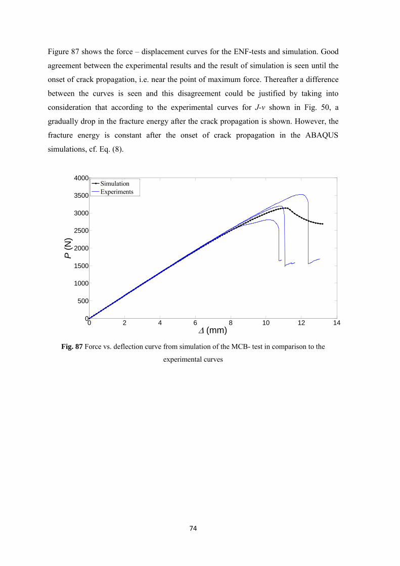
74

Figure 87 shows the force – displacement curves for the ENF-tests and simulation. Good

agreement between the experimental results and the result of simulation is seen until the

onset of crack propagation, i.e. near the point of maximum force. Thereafter a difference

between the curves is seen and this disagreement could be justified by taking into

consideration that according to the experimental curves for J-v shown in Fig. 50, a

gradually drop in the fracture energy after the crack propagation is shown. However, the

fracture energy is constant after the onset of crack propagation in the ABAQUS

simulations, cf. Eq. (8).

Fig. 87 Force vs. deflection curve from simulation of the MCB- test in comparison to the

experimental curves

0 2 4 6 8 10 12 140

500

1000

1500

2000

2500

3000

3500

4000

(mm)

P (

N)

SimulationExperiments

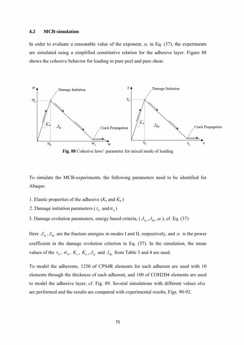
75

4.2 MCB-simulation

In order to evaluate a reasonable value of the exponent, α, in Eq. (37), the experiments

are simulated using a simplified constitutive relation for the adhesive layer. Figure 88

shows the cohesive behavior for loading in pure peel and pure shear.

Fig. 88 Cohesive laws’ parameter for mixed mode of loading

To simulate the MCB-experiments, the following parameters need to be identified for

Abaqus:

1. Elastic properties of the adhesive (Ks and Kn )

2. Damage initiation parameters ( 0 and 0 )

3. Damage evolution parameters, energy based criteria, ( IcJ , IIcJ , ), cf. Eq. (37)

Here IcJ , IIcJ are the fracture energies in modes I and II, respectively, and is the power

coefficient in the damage evolution criterion in Eq. (37). In the simulation, the mean

values of the 0 , 0 , sK , nK , IcJ and IIcJ from Table 3 and 4 are used.

To model the adherents, 1250 of CPS4R elements for each adherent are used with 10

elements through the thickness of each adherent, and 100 of COH2D4 elements are used

to model the adhesive layer, cf. Fig. 89. Several simulations with different values of are performed and the results are compared with experimental results, Figs. 90-92.

JIIc JIc

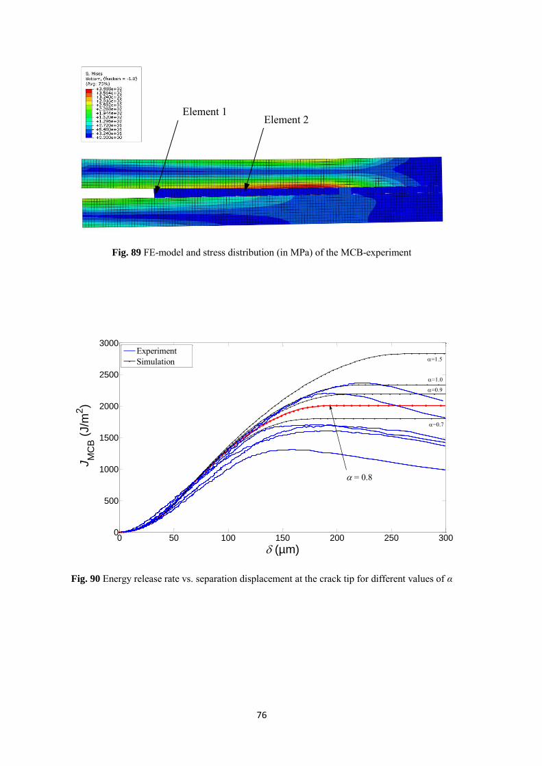
76

Fig. 89 FE-model and stress distribution (in MPa) of the MCB-experiment

Fig. 90 Energy release rate vs. separation displacement at the crack tip for different values of α

0 50 100 150 200 250 3000

500

1000

1500

2000

2500

3000

(µm)

JM

CB (

J/m

2)

=0.7

= 0.8

=0.9

=1.0

=1.5ExperimentSimulation

Element 1 Element 2

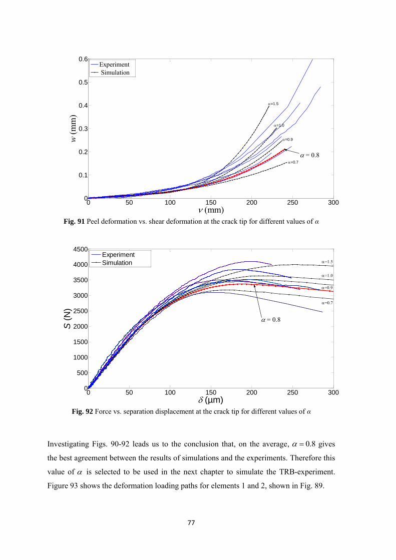
77

Fig. 91 Peel deformation vs. shear deformation at the crack tip for different values of α

Fig. 92 Force vs. separation displacement at the crack tip for different values of α

Investigating Figs. 90-92 leads us to the conclusion that, on the average, 0.8 gives

the best agreement between the results of simulations and the experiments. Therefore this

value of is selected to be used in the next chapter to simulate the TRB-experiment.

Figure 93 shows the deformation loading paths for elements 1 and 2, shown in Fig. 89.

0 50 100 150 200 250 3000

0.1

0.2

0.3

0.4

0.5

0.6

(mm)

w (m

m)

=0.7

= 0.8

=0.9

=1.0

=1.5

Experiment Simulation

0 50 100 150 200 250 3000

500

1000

1500

2000

2500

3000

3500

4000

4500

(µm)

S (

N)

=0.7

= 0.8

=0.9

=1.0

=1.5Experiment

Simulation

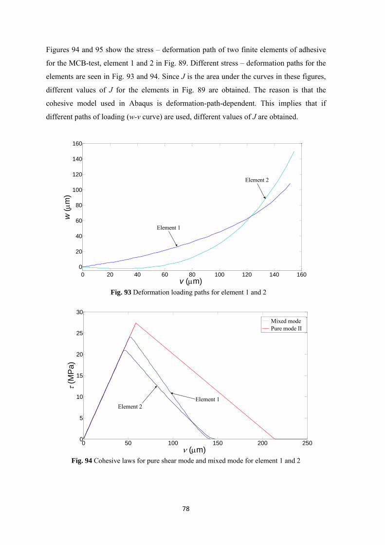
78

Figures 94 and 95 show the stress – deformation path of two finite elements of adhesive

for the MCB-test, element 1 and 2 in Fig. 89. Different stress – deformation paths for the

elements are seen in Fig. 93 and 94. Since J is the area under the curves in these figures,

different values of J for the elements in Fig. 89 are obtained. The reason is that the

cohesive model used in Abaqus is deformation-path-dependent. This implies that if

different paths of loading (w-v curve) are used, different values of J are obtained.

Fig. 93 Deformation loading paths for element 1 and 2

Fig. 94 Cohesive laws for pure shear mode and mixed mode for element 1 and 2

0 20 40 60 80 100 120 140 160

0

20

40

60

80

100

120

140

160

v (m)

w (

m)

Element 1

Element 2

0 50 100 150 200 2500

5

10

15

20

25

30

(m)

(M

Pa

)

Mixed mode Pure mode II

Element 2Element 1

79

Fig. 95 Cohesive laws for the pure peel mode and mixed mode for element 1 and 2

Figure 96 shows the comparison between J obtained by integration of the cohesive law at

the crack tip element, Eq. (2) and JMCB obtained by Eq. (21). Good agreement is observed

until the onset of crack propagation. Thereafter a difference between the curves is seen.

The origin for this disagreement can be the load path dependent fracture energy in

Abaqus’ cohesive model as discussed above. The fact that the model is deformation path

dependent implies that the J-integral is not integration path dependent. Thus, the accuracy

of Eq. (21) cannot be guaranteed.

Fig. 96 Energy release rate vs. separation displacement at the crack tip for the MCB specimen

by Eq. (2) and Eq. (21)

0 50 100 1500

5

10

15

20

25

w (m)

(

MP

a)

Mixed mode Pure mode I

Element 2

Element 1

0 100 200 300 400 500 600 700 8000

500

1000

1500

2000

2500

(µm)

JM

CB (

J/m

2)

JMCB by Eq. (2)

JMCB by Eq. (21)

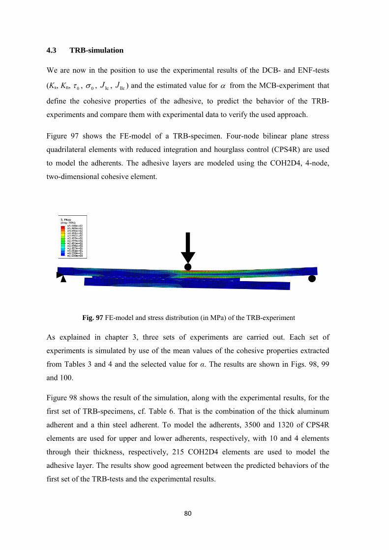
80

4.3 TRB-simulation

We are now in the position to use the experimental results of the DCB- and ENF-tests

(Ks, Kn, 0 , 0 , IcJ , IIcJ ) and the estimated value for from the MCB-experiment that

define the cohesive properties of the adhesive, to predict the behavior of the TRB-

experiments and compare them with experimental data to verify the used approach.

Figure 97 shows the FE-model of a TRB-specimen. Four-node bilinear plane stress

quadrilateral elements with reduced integration and hourglass control (CPS4R) are used

to model the adherents. The adhesive layers are modeled using the COH2D4, 4-node,

two-dimensional cohesive element.

Fig. 97 FE-model and stress distribution (in MPa) of the TRB-experiment

As explained in chapter 3, three sets of experiments are carried out. Each set of

experiments is simulated by use of the mean values of the cohesive properties extracted

from Tables 3 and 4 and the selected value for α. The results are shown in Figs. 98, 99

and 100.

Figure 98 shows the result of the simulation, along with the experimental results, for the

first set of TRB-specimens, cf. Table 6. That is the combination of the thick aluminum

adherent and a thin steel adherent. To model the adherents, 3500 and 1320 of CPS4R

elements are used for upper and lower adherents, respectively, with 10 and 4 elements

through their thickness, respectively, 215 COH2D4 elements are used to model the

adhesive layer. The results show good agreement between the predicted behaviors of the

first set of the TRB-tests and the experimental results.

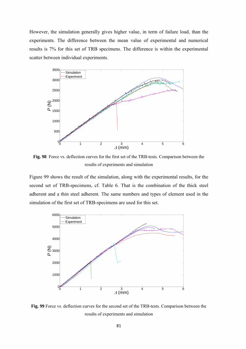
81

However, the simulation generally gives higher value, in term of failure load, than the

experiments. The difference between the mean value of experimental and numerical

results is 7% for this set of TRB specimens. The difference is within the experimental

scatter between individual experiments.

Fig. 98 Force vs. deflection curves for the first set of the TRB-tests. Comparison between the

results of experiments and simulation

Figure 99 shows the result of the simulation, along with the experimental results, for the

second set of TRB-specimens, cf. Table 6. That is the combination of the thick steel

adherent and a thin steel adherent. The same numbers and types of element used in the

simulation of the first set of TRB-specimens are used for this set.

Fig. 99 Force vs. deflection curves for the second set of the TRB-tests. Comparison between the

results of experiments and simulation

0 1 2 3 4 5 60

500

1000

1500

2000

2500

3000

3500

(mm)

P (

N)

Simulation

Experiment

0 1 2 3 4 5 60

1000

2000

3000

4000

5000

6000

(mm)

P (

N)

Simulation

Experiment

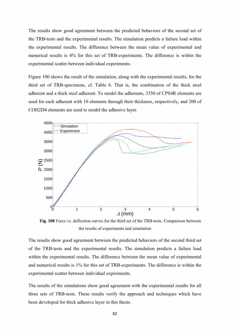
82

The results show good agreement between the predicted behaviors of the second set of

the TRB-tests and the experimental results. The simulation predicts a failure load within

the experimental results. The difference between the mean value of experimental and

numerical results is 4% for this set of TRB-experiments. The difference is within the

experimental scatter between individual experiments.

Figure 100 shows the result of the simulation, along with the experimental results, for the

third set of TRB-specimens, cf. Table 6. That is, the combination of the thick steel

adherent and a thick steel adherent. To model the adherents, 3350 of CPS4R elements are

used for each adherent with 10 elements through their thickness, respectively, and 200 of

COH2D4 elements are used to model the adhesive layer.

Fig. 100 Force vs. deflection curves for the third set of the TRB-tests. Comparison between

the results of experiments and simulation

The results show good agreement between the predicted behaviors of the second third set

of the TRB-tests and the experimental results. The simulation predicts a failure load

within the experimental results. The difference between the mean value of experimental

and numerical results is 1% for this set of TRB-experiments. The difference is within the

experimental scatter between individual experiments.

The results of the simulations show good agreement with the experimental results for all

three sets of TRB-tests. These results verify the approach and techniques which have

been developed for thick adhesive layer in this thesis.

0 1 2 3 4 5 60

500

1000

1500

2000

2500

3000

3500

4000

4500

(mm)

P (

N)

Simulation

Experiment

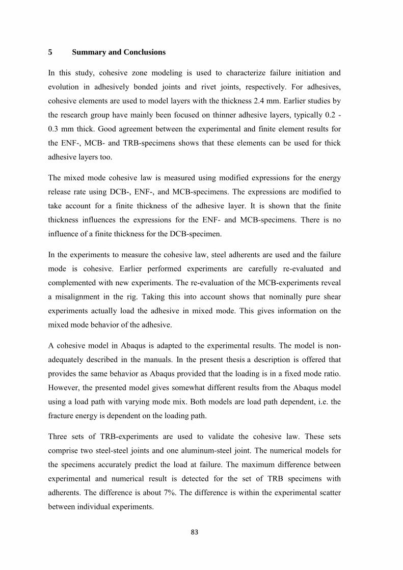
83

5 Summary and Conclusions

In this study, cohesive zone modeling is used to characterize failure initiation and

evolution in adhesively bonded joints and rivet joints, respectively. For adhesives,

cohesive elements are used to model layers with the thickness 2.4 mm. Earlier studies by

the research group have mainly been focused on thinner adhesive layers, typically 0.2 -

0.3 mm thick. Good agreement between the experimental and finite element results for

the ENF-, MCB- and TRB-specimens shows that these elements can be used for thick

adhesive layers too.

The mixed mode cohesive law is measured using modified expressions for the energy

release rate using DCB-, ENF-, and MCB-specimens. The expressions are modified to

take account for a finite thickness of the adhesive layer. It is shown that the finite

thickness influences the expressions for the ENF- and MCB-specimens. There is no

influence of a finite thickness for the DCB-specimen.

In the experiments to measure the cohesive law, steel adherents are used and the failure

mode is cohesive. Earlier performed experiments are carefully re-evaluated and

complemented with new experiments. The re-evaluation of the MCB-experiments reveal

a misalignment in the rig. Taking this into account shows that nominally pure shear

experiments actually load the adhesive in mixed mode. This gives information on the

mixed mode behavior of the adhesive.

A cohesive model in Abaqus is adapted to the experimental results. The model is non-

adequately described in the manuals. In the present thesis a description is offered that

provides the same behavior as Abaqus provided that the loading is in a fixed mode ratio.

However, the presented model gives somewhat different results from the Abaqus model

using a load path with varying mode mix. Both models are load path dependent, i.e. the

fracture energy is dependent on the loading path.

Three sets of TRB-experiments are used to validate the cohesive law. These sets

comprise two steel-steel joints and one aluminum-steel joint. The numerical models for

the specimens accurately predict the load at failure. The maximum difference between

experimental and numerical result is detected for the set of TRB specimens with

adherents. The difference is about 7%. The difference is within the experimental scatter

between individual experiments.

84

Thus, it appears safe to extract a cohesive law using one set of adherents and use it for

other adherents and even mixed adherents. At least as long as the failure mode is

cohesive.

The other issue studied in this thesis is the failure behavior of riveted joints. A method is

proposed for structural analysis of rivet joints using cohesive modeling. A theoretical and

numerical study supports the idea. It indicates that a modified DCB-specimen can be used

to measure the cohesive properties. It should be noted that these properties are used to

model a fracture process that is essentially governed by plasticity. The advantage with the

cohesive model is its possible ability to model a complex process using rather large-scale

finite elements. The numerical study of the riveted DCB-specimen shows that the joint

essentially acts as a continuous joint if the distance between the rivets is small enough.

The conclusion of this work is that cohesive zone modeling is a powerful technique to

study the failure behavior of adhesively bonded joint with thick adhesive layer. The

preliminary study of rivet joints indicates a good prospect to use the method for this type

joints as well.

85

References

ABAQUS, General-Purpose Finite Element System, Hibbit, Karlson&Sorensen Inc., 100

Medway Street, Providence, RI., 1997.

Abaqus® Documentation (2011) Dassault Systèmes, Vélizy-Villacoublay

Afendi, M. and Teramoto, T. (2009) ‘Fracture toughness test of epoxy adhesive

dissimilar joint with various adhesive. Journal of Solid Mechanics and

Materials Engineering (JSME), 4 (7), pp. 999-1010, 2010.

Alfredsson, K.S. (2004) ‘On the instantaneous energy release rate of the end-notch

flexure adhesive joint specimen’, International Journal of Solids and

Structures 41:4787-4807.

Alfredsson, K.S., Gillespie, J.W., Bogetti, T.A., Carlsson, L.A. and Yiournas, A. (2008)

‘Flexure beams with interlayer- symmetric beams with orthotropic adherents’,

Journal of Mechanics of Materials and Structures 3, 45-62.

Andersson, T. and Stigh, U. (2004) ‘The stress-elongation relation for an adhesive layer

loaded in peel using equilibrium of energetic forces’, Int. J. of Solids and

Struct. 41:413-434.

Andersson, T. and Biel, A. (2006) ‘On the effective constitutive properties of a thin

adhesive layer loaded in peel’, Int. J. Frac. (2006) 141:227–246.

André, A., Haghani, R. and Biel, A. (2012) ‘Application of fracture mechanics to predict

the failure load of adhesive joints used to bond CFRP laminates to steel

members’, Journal of Construction and Buildings Materials.

Barenblatt, G.I. (1959) ‘The formation of Equilibrium cracks during brittle fracture’, J.

Appl. Math. Mech., vol. 23, no. 3, 1959, pp. 434-444.

Barenblatt, G.I. (1962) ‘The mathematical theory of equilibrium cracks in brittle

fracture’, Adv. Appl. Mech. 7:55-129.

Biel, A. (2005) ‘Constitutive behavior and fracture toughness of an adhesive layer’,

Thesis for the degree of licentiate in engineering, Chalmers University of

Technology.

Broek, D. (1982) Elementary engineering fracture mechanics, Springer: first edition.

Brockmann, W.,Geiss, P.L, Kligen, J. and Schröder, B. (2009) Adhesive Bonding:

Materials, Applications and Technology WILEY-VCH Verlag GmbH & Co.

KGaA, Weinheim, ISBN: 978-3-527-31898-8

86

Camanho, P. and Davila, C. (2002) ‘ Mixed-mode decohesion finite elements for the

simulation of delamination in composite materials’,NASA/TM-2002-211737.

Chandra, N., Li, H., Shet, C. and Ghonem, H. (2002) ‘Some issues in the application of

cohesive zone models for metal–ceramic interfaces’, Int. J. Solids Struct. 39,

2827-2855.

Choupani, N. (2008) ‘Mixed-mode cohesive fracture of adhesive joints: Experimental

and numerical studies’, Journal of Engineering Fracture Mechanics 75 4363-

4382.

Coulomb, C.A. (1776) ‘Remarque sur la rupture des corps’, Memoires presentes par

divers savants a l’Academie, vol. 7.

Cui, W. and Wisnom, M.R. (1993) ‘A combined stress-based and fracture-mechanics-

based model forpredicting delamination in composites’, Composites 24, 467-

474.

da Silva, L.F.M. and Campilho, R.D.S.G (2012) Advances in Numerical Modeling of

Adhesive joints , Springer, ISBN 978-3-642-23607-5.

Dugdale, D.S. (1960) ‘Yielding of steel sheets containing slits’, J. Mech. Phys. Solids,

100-104.

Eshelby, J.D. ‘The Force on Elastic Singularity’, Philos. Trans. Roy. Soc. London A, 244,

87 (1951).

Fleck, N A, Hutchinson, J. and Suo Z. (1991) ‘Crack path selection in a brittle adhesive

layer’, Int. J. of Solids and Structures, 27(13), pp 1683-1703.

Forman, R.G (1967) ‘Effect of plastic deformation on the strain energy release rate in a

centrally notched plate subjected to uniaxial tension’, ASME paper 65

WA/MET/9.

Gerken, J.M., Bennett, J. and Smith, F. (2001) ‘Numerical Simulation of the

Mechanically Coupled Cook-Off Experiment’, Journal of Materials and

Technology: Transaction of the American Society of Mechanical Engineers.

Griffith, A.A. (1920) ‘The phenomena of rupture and flow of solids’, Phil.Trans. Roy.

Soc. London.

Högberg, J.L. and Stigh, U. (2006) ‘Specimen proposals for mixed mode testing of

adhesive layer’, Engineering Fracture Mechanics 73, 2541-2587.

Högberg, J.L., Sørensen, B.F. and Stigh, U. (2007) ‘Constitutive behavior of mixed mode

loaded adhesive layer’, International Journal of Solids and Structures,

Volume 44, pp. 8335–8354

87

Inglis, C.E. (1913) ‘Stresses in plate due to presence of crack and sharp corners,

Proceedings-Institute of Naval Architect, 60.

Irwin, G.R. (1948) ‘Fracture Dynamics. In Fracturing of Metals’, 147-166. 1947 ASM

Symposium (Trans. ASM 40A), Cleveland.

Irwin, G. R. (1957) ‘Analysis of stresses and strains near the end of a crack traversing a

plate’, J. of Applied Mechanics, A.S.M.E., N. Y.

Kafkalidis, M.S. and Thouless, M.D. (2002) ‘The effects of geometry and material

properties on the fracture of single lap-shear joints’, Int. J. Solids Struct. 39,

4367-4383.

Kinloch, A.J. (1987) Adhesion and Adhesives: Science and Technology (Chapman and

Hall, London).

Kirsch, G., (1898) ‘Die Theorie der Elastizität und di Bedürfnisse der Festigkeitslehre’,

Zeitschrift de Vereines deutscher Ingenieure 42 (28): 797–807.

Klarbring, A. (1991) ‘Derivation of the model of adhesively bonded joints by the

asymptotic expansion method’, Int. J. of Engineering Science 29,493-512.

Leffler, K., Alfredsson, K.S. and Stigh, U. (2007) ‘Shear behavior of adhesive layers’,

Int. J. of Solids and Struct. 44:530-545.

Mi, Y., Crisfield, M.A., Davies, G.A.O. and Hellweg, H.B. (1998) ‘Progressive

delamination using interface elements’, J. Compos. Mater. 32, 1246-1272.

Needleman, A. (1987) ‘A Continuum Model for Void Nucleation by Inclusion

Debonding’, Journal of Applied Mechanics 1987; 54: 525-531.

Olsson, P. and Stigh, U. (1989) ‘On the determination of the constitutive properties of

thin interphase layers an exact inverse solution’, Int. J. of Fract. Mec.

41(4):R71-R76.

Pinto, A.M.G., Magalhães, A.G., Campilho, R.D.S.G., de Moura, M.F.S.F. and Baptista,

A.P.M. (2009) ‘Single lap joints of similar and dissimilar adherends bonded

with an acrylic adhesive’, J. Adhes. 85,351-376.

Razvan, R. (2009) ‘ Some remarks on the history of fracture mechanics’, Proceedings of

the 3rd International Conference on Applied Mathematics, Simulation,

Modeling, Circuits, Systems and Signals Pages 122-131.

Rice, J.R. (1968) ‘A path independent integral and the approximative analysis of strain

concentration by notches and cracks’, ASME J. App. Mech., 88, 379-386.

88

Robinson, J.N (1977) ‘An experimental investigation of the effect of specimen type on

the crack tip opening displacement and J-integral fracture criteria’, Int. J. of

fracture, 12 pp.723 737.

Stigh, U. (1987) ‘Initiation and growth of an interface crack. Mechanical behavior of

adhesive joints’, Pluralis, Paris, France, pp. 237-248

Sun, C.T., Jin, Z.H. (2011) Fracture Mechanics, Elsevier, ISBN 978-0-12-385001-01.

Sørensen, B.F. (2002) ‘Cohesive law and notch sensitivity of adhesive joints’, Acta

Mater. 50, 1053-1061.

Sørensen, B.F. and Jacobsen, T.K. (2003) ‘Determination of cohesive laws by the J

integral approach’, Eng. Fract. Mech. 70, 1841-1858.

Sørensen, B.F., Kirkegaard, P. (2006) ‘Determination of mixed mode cohesive laws’,

Eng. Fract. Mech. 73, 2642–2661

Volkersen, O. (1938) ‘Die nietkraftverteilung in zubeanspruchten nietverbindungen mit

konstanten laschenquerschnitten’, Luftfahrtforschung 15, 41-47.

Weinberger, C., Cai, W. and Barnett, D. (2005) Lecture Notes – Elasticity of Microscopic

Structures, Stanford University.

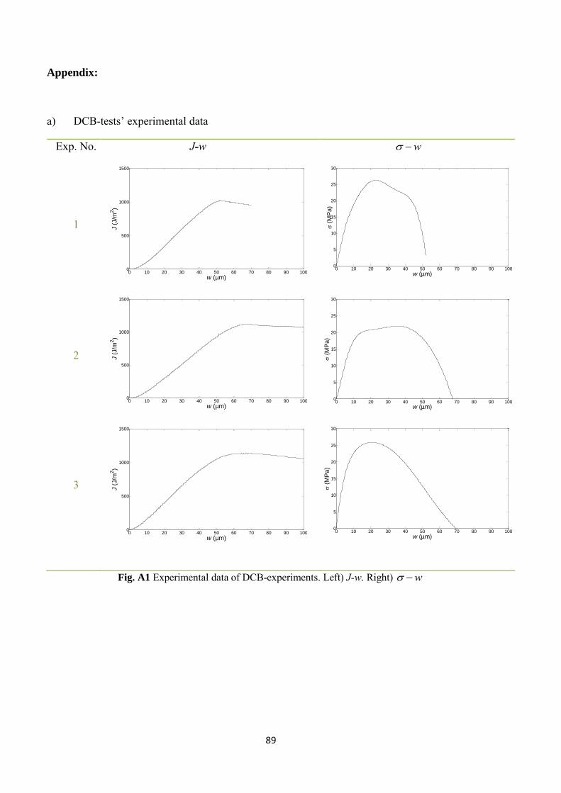
89

Appendix:

a) DCB-tests’ experimental data

Exp. No. J-w w

1

2

3

Fig. A1 Experimental data of DCB-experiments. Left) J-w. Right) w

0 10 20 30 40 50 60 70 80 90 1000

500

1000

1500

w (µm)

J (

J/m

2)

0 10 20 30 40 50 60 70 80 90 1000

5

10

15

20

25

30

w (µm)

(

MP

a)

0 10 20 30 40 50 60 70 80 90 1000

500

1000

1500

w (µm)

J (

J/m

2)

0 10 20 30 40 50 60 70 80 90 1000

5

10

15

20

25

30

w (µm)

(

MP

a)

0 10 20 30 40 50 60 70 80 90 1000

500

1000

1500

w (µm)

J (

J/m

2)

0 10 20 30 40 50 60 70 80 90 1000

5

10

15

20

25

30

w (µm)

(

MP

a)

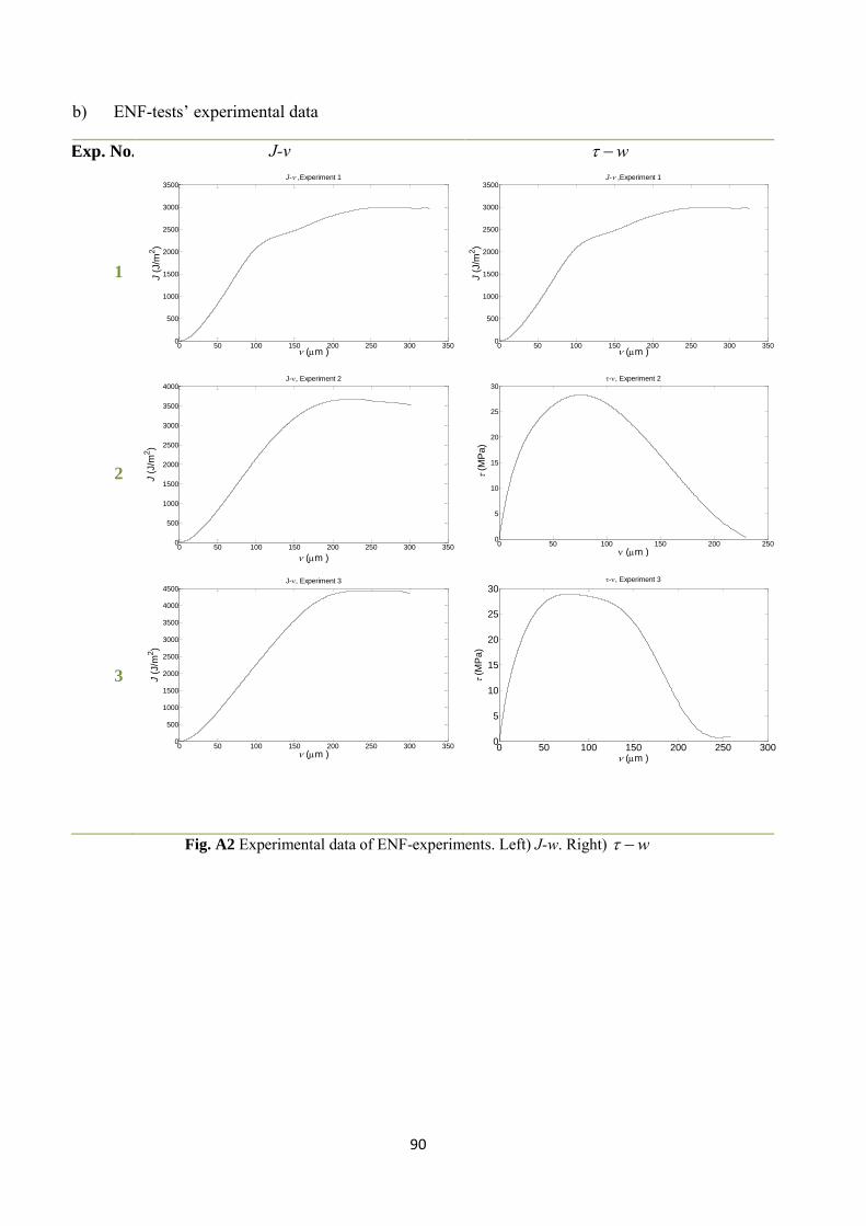
90

b) ENF-tests’ experimental data

Exp. No. J-v w

1

2

3

Fig. A2 Experimental data of ENF-experiments. Left) J-w. Right) w

0 50 100 150 200 250 300 3500

500

1000

1500

2000

2500

3000

3500J- ,Experiment 1

(m )

J (

J/m

2)

0 50 100 150 200 250 300 3500

500

1000

1500

2000

2500

3000

3500J- ,Experiment 1

(m )

J (

J/m

2)

0 50 100 150 200 250 300 3500

500

1000

1500

2000

2500

3000

3500

4000J-, Experiment 2

(m )

J (

J/m

2)

0 50 100 150 200 2500

5

10

15

20

25

30-, Experiment 2

(m )

(M

Pa

)

0 50 100 150 200 250 300 3500

500

1000

1500

2000

2500

3000

3500

4000

4500J-, Experiment 3

(m )

J (

J/m

2)

0 50 100 150 200 250 3000

5

10

15

20

25

30-, Experiment 3

(m )

(M

Pa)

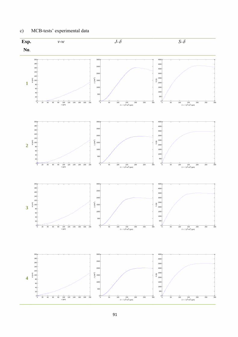
91

c) MCB-tests’ experimental data

Exp..

No.

v-w J- S-

1

2

3

4

0 20 40 60 80 100 120 140 160 180 2000

20

40

60

80

100

120

140

160

180

200

(µm)

w (

µm

)

0 50 100 150 200 250 3000

500

1000

1500

2000

2500

3000

= (v2+w2) (µm)

J (

J/M

2)

0 50 100 150 200 250 3000

500

1000

1500

2000

2500

3000

3500

4000

4500

= (v2+w2) (µm)

S (

N)

0 20 40 60 80 100 120 140 160 180 2000

20

40

60

80

100

120

140

160

180

200

(µm)

w (

µm

)

0 50 100 150 200 250 3000

500

1000

1500

2000

2500

3000

= (v2+w2) (µm)

J (

J/M

2)

0 50 100 150 200 250 3000

500

1000

1500

2000

2500

3000

3500

4000

4500

= (v2+w2) (µm)

S (

N)

0 20 40 60 80 100 120 140 160 180 2000

20

40

60

80

100

120

140

160

180

200

(µm)

w (

µm

)

0 50 100 150 200 250 3000

500

1000

1500

2000

2500

3000

= (v2+w2) (µm)

J (

J/M

2)

0 50 100 150 200 250 3000

500

1000

1500

2000

2500

3000

3500

4000

4500

= (v2+w2) (µm)

S (

N)

0 20 40 60 80 100 120 140 160 180 2000

20

40

60

80

100

120

140

160

180

200

(µm)

w (

µm

)

0 50 100 150 200 250 3000

500

1000

1500

2000

2500

3000

= (v2+w2) (µm)

J (

J/M

2)

0 50 100 150 200 250 3000

500

1000

1500

2000

2500

3000

3500

4000

4500

= (v2+w2) (µm)

S (

N)

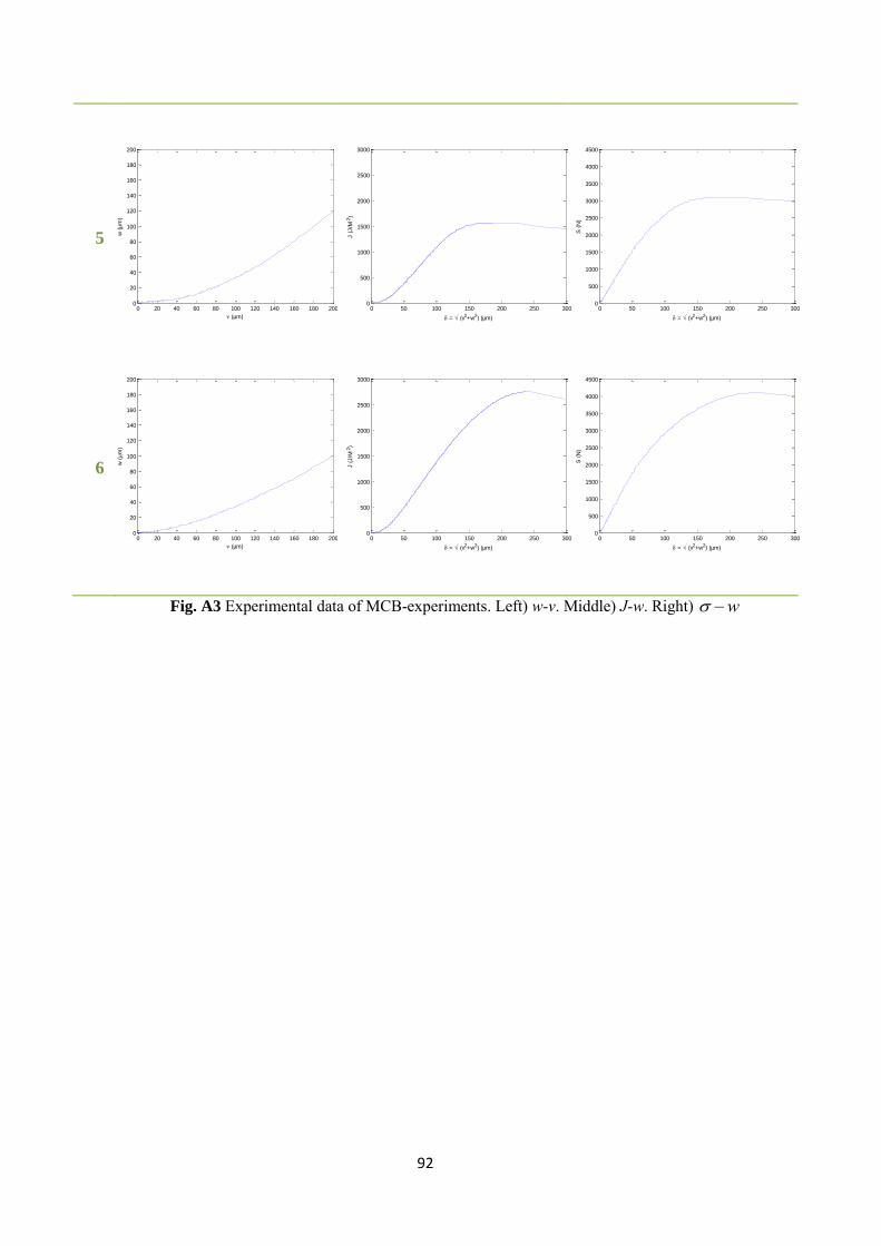
92

5

6

Fig. A3 Experimental data of MCB-experiments. Left) w-v. Middle) J-w. Right) w

0 20 40 60 80 100 120 140 160 180 2000

20

40

60

80

100

120

140

160

180

200

(µm)

w (

µm

)

0 50 100 150 200 250 3000

500

1000

1500

2000

2500

3000

= (v2+w2) (µm)

J (

J/M

2)

0 50 100 150 200 250 3000

500

1000

1500

2000

2500

3000

3500

4000

4500

= (v2+w2) (µm)

S (

N)

0 20 40 60 80 100 120 140 160 180 2000

20

40

60

80

100

120

140

160

180

200

(µm)

w (

µm

)

0 50 100 150 200 250 3000

500

1000

1500

2000

2500

3000

= (v2+w2) (µm)

J (

J/M

2)

0 50 100 150 200 250 3000

500

1000

1500

2000

2500

3000

3500

4000

4500

= (v2+w2) (µm)

S (

N)

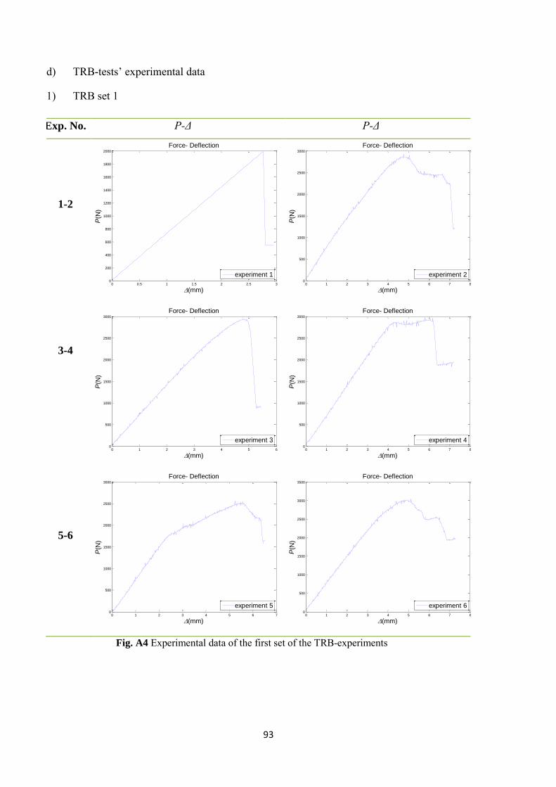
93

d) TRB-tests’ experimental data

1) TRB set 1

Exp. No. P-Δ P-Δ

1-2

3-4

5-6

Fig. A4 Experimental data of the first set of the TRB-experiments

0 0.5 1 1.5 2 2.5 30

200

400

600

800

1000

1200

1400

1600

1800

2000

Force- Deflection

(mm)

P(N

)

experiment 1

0 1 2 3 4 5 6 7 80

500

1000

1500

2000

2500

3000

Force- Deflection

(mm)P

(N)

experiment 2

0 1 2 3 4 5 60

500

1000

1500

2000

2500

3000

Force- Deflection

(mm)

P(N

)

experiment 3

0 1 2 3 4 5 6 7 80

500

1000

1500

2000

2500

3000

Force- Deflection

(mm)

P(N

)

experiment 4

0 1 2 3 4 5 6 70

500

1000

1500

2000

2500

3000

Force- Deflection

(mm)

P(N

)

experiment 5

0 1 2 3 4 5 6 7 80

500

1000

1500

2000

2500

3000

3500

Force- Deflection

(mm)

P(N

)

experiment 6

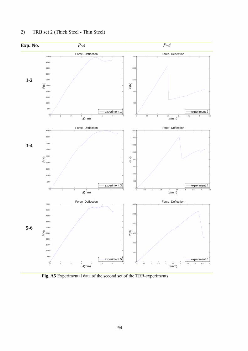
94

2) TRB set 2 (Thick Steel - Thin Steel)

Exp. No. P-Δ P-Δ

1-2

3-4

5-6

Fig. A5 Experimental data of the second set of the TRB-experiments

0 1 2 3 4 5 6 70

500

1000

1500

2000

2500

3000

3500

4000

4500

5000

Force- Deflection

(mm)

P(N

)

experiment 1

0 0.5 1 1.5 2 2.5 3 3.50

500

1000

1500

2000

2500

Force- Deflection

(mm)

P(N

)

experiment 2

0 1 2 3 4 5 60

500

1000

1500

2000

2500

3000

3500

4000

4500

Force- Deflection

(mm)

P(N

)

experiment 3

0 0.5 1 1.5 2 2.5 3 3.5 4 4.50

500

1000

1500

2000

2500

3000

3500

4000

Force- Deflection

(mm)

P(N

)

experiment 4

0 1 2 3 4 5 6 70

500

1000

1500

2000

2500

3000

3500

4000

4500

5000

Force- Deflection

(mm)

P(N

)

experiment 5

0 0.5 1 1.5 2 2.5 3 3.5 4 4.5 50

1000

2000

3000

4000

5000

6000

Force- Deflection

(mm)

P(N

)

experiment 6

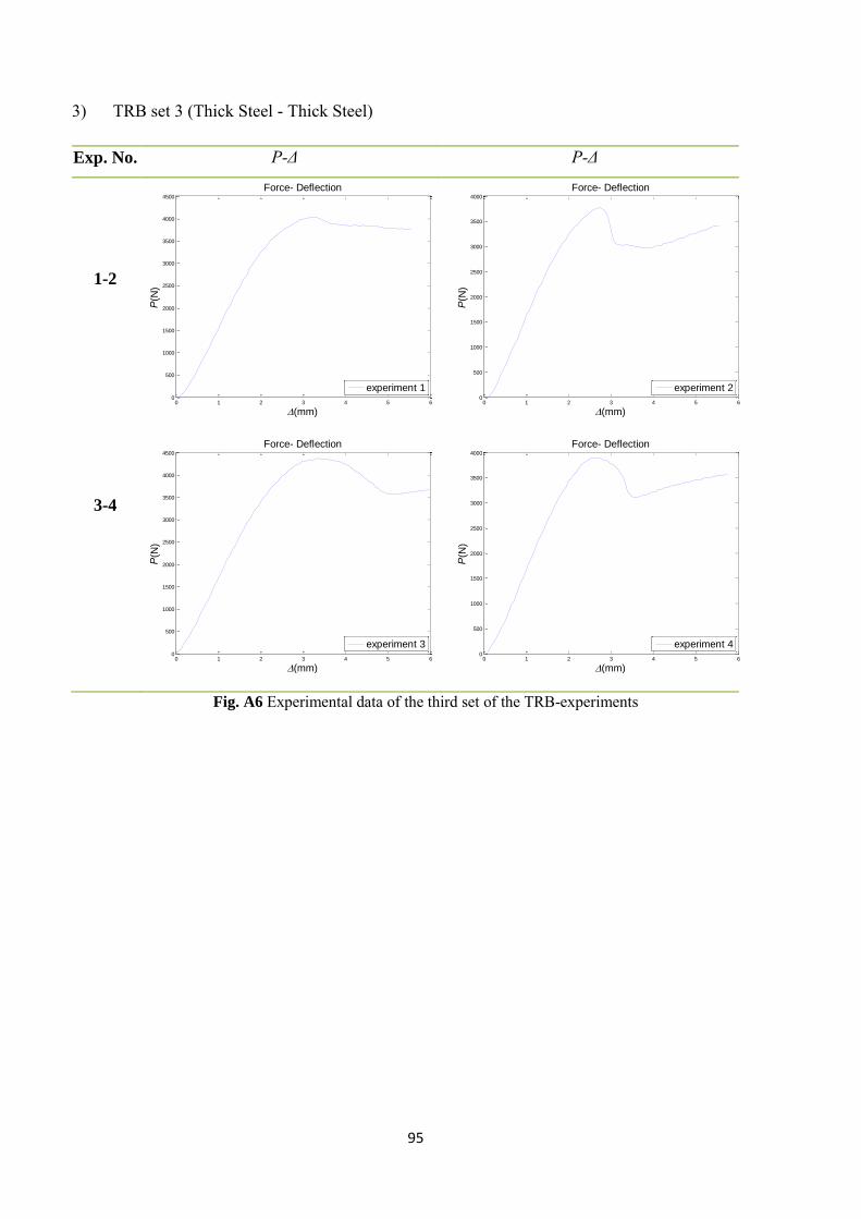
95

3) TRB set 3 (Thick Steel - Thick Steel)

Exp. No. P-Δ P-Δ

1-2

3-4

Fig. A6 Experimental data of the third set of the TRB-experiments

0 1 2 3 4 5 60

500

1000

1500

2000

2500

3000

3500

4000

4500

Force- Deflection

(mm)

P(N

)

experiment 1

0 1 2 3 4 5 60

500

1000

1500

2000

2500

3000

3500

4000

Force- Deflection

(mm)

P(N

)

experiment 2

0 1 2 3 4 5 60

500

1000

1500

2000

2500

3000

3500

4000

4500

Force- Deflection

(mm)

P(N

)

experiment 3

0 1 2 3 4 5 60

500

1000

1500

2000

2500

3000

3500

4000

Force- Deflection

(mm)

P(N

)

experiment 4

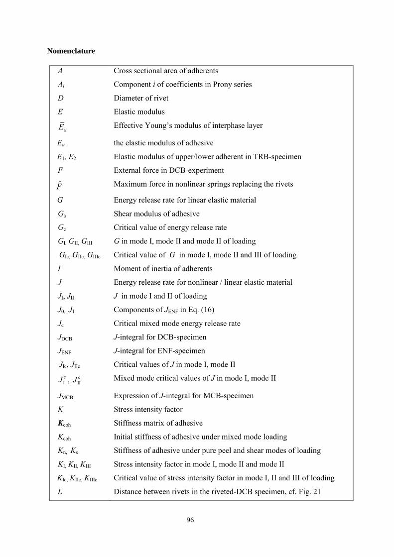
96

Nomenclature

A Cross sectional area of adherents

Ai Component i of coefficients in Prony series

D Diameter of rivet

E Elastic modulus

aE Effective Young’s modulus of interphase layer

Ea the elastic modulus of adhesive

E1, E2 Elastic modulus of upper/lower adherent in TRB-specimen

F External force in DCB-experiment

F Maximum force in nonlinear springs replacing the rivets

G Energy release rate for linear elastic material

Ga Shear modulus of adhesive

Gc Critical value of energy release rate

GI, GII, GIII G in mode I, mode II and mode II of loading

GIc, GIIc, GIIIc Critical value of G in mode I, mode II and III of loading

I Moment of inertia of adherents

J Energy release rate for nonlinear / linear elastic material

JI, JII J in mode I and II of loading

J0, J1 Components of JENF in Eq. (16)

Jc Critical mixed mode energy release rate

JDCB J-integral for DCB-specimen

JENF J-integral for ENF-specimen

JIc, JIIc Critical values of J in mode I, mode II

cIJ , c

IIJ Mixed mode critical values of J in mode I, mode II

JMCB Expression of J-integral for MCB-specimen

K Stress intensity factor

Kcoh Stiffness matrix of adhesive

Kcoh Initial stiffness of adhesive under mixed mode loading

Kn, Ks Stiffness of adhesive under pure peel and shear modes of loading

KI, KII, KIII Stress intensity factor in mode I, mode II and mode II

KIc, KIIc, KIIIc Critical value of stress intensity factor in mode I, II and III of loading

L Distance between rivets in the riveted-DCB specimen, cf. Fig. 21

97

M External bending moment, cf. Fig. 3

M1, M2 Internal bending moments on the integration paths, cf. Fig. 16b

1M , 2M External bending moments, cf. Fig. 16a

N Uniaxial force, cf. Fig. 9

P External force in ENF- and TRB-experiments, cf. Fig. 12

P1, P2 External forces in Fig. 3

S External force in MCB-experiments, cf. Fig. 15

SP Slope of the curves in Fig. 67

Ti Component i of traction vector

T0 Cohesive strength in mixed mode, cf. Fig. 29

V Shear force, cf. Fig. 16

W Density of the strain energy

a Crack length

a0 Initial crack length

b Width of specimen, cf. Fig. 56

c Distance from crack tip to loading point in ENF-test

d Damage parameter

db Bonded length of adherents, cf. Fig. 63

g Unbonded gap for spacers, cf. Fig. 63

h Height of adherents, cf. Fig. 9

h1,h2 Height of upper/lower adherent, cf. Fig. 63

hs Height of reinforcing bar in Fig. 20

k Number of terms in Prony and polynomial series

l Length of specimen

l1, l2 Length of lower/upper bar in TRB-specimen, cf. Fig. 63

l Distance between integration paths and loading points in Fig. 9

nj Unit vector normal to integration path of J along xj direction

nx, ny Unit normal vector to the J-integral contour along x/y direction

o Length of overhang part of bars in ENF- and TRB-specimens

t Thickness of adhesive layer, cf. Fig. 9

ts Thickness of sheet metal in Fig. 20

ux,1, ux,2 Displacement of points 1 and 2 along x direction, cf. Fig. 58

ux,3, ux,4 Displacement of points 3 and 4 along x direction, cf. Fig. 58

98

uy,2, uy,3 Displacement of points 2 / 3 along y direction, cf. Fig. 58

ui Displacement along xi direction

v Shear deformation of the adhesive layer

v Shear deformation as an integration variable

v0 Shear displacement of the adhesive corresponding to peek strength

vc Failure displacement along shear direction, cf. Fig. 31

w Peel deformation of the adhesive layer

w Peel deformation as an integration variable

w Rotation of the beam, cf. Fig. 14

w0 Peel deformation of the adhesive corresponding to peek strength

wc Failure displacement along peel direction, cf. Fig. 81

x, y, z Spatial coordinates, cf. Fig. 2

x1, x2 Spatial coordinates, cf. Fig. 3

y1, y2, y3, y4 Coordinate of point 1, 2, 3 and 4 along y-axis, cf. Fig. 58

α Power coefficient in Eq. (37)

β Loading angle in MCB-experiment, cf. Fig. 15

Displacement of loading point

Rate of the displacement of the loading point

δ Separation displacement of adhesive in mixed mode

δ0 Mixed mode separation displacement corresponding to peek strength

δc Mixed mode separation displacement corresponding to decohesion

δmax Maximum mixed mode separation displacement

ε In-plane strain vector

εij Components of strain tensor

εxx, εyy Normal strain along x/y direction

γc Critical surface energy per unit area of the crack

γxy Shear strain in x-y plane

Mixed mode ratio

Coefficient in CTOD expression

va Poisson ration of adhesive

Π Total potential energy per unit thickness of system Loading path direction variable

Peel stress

99

Maximum stress in nonlinear springs

0 Peel strength of adhesive

ij Component of stress tensor

xx , yy Normal stresses along x/y direction

y y, Normal / shear yield stress

Shear stress

max Strength of adhesive under pure shear mode of loading

Constant shear stress in Eq. (10)

ave Average shear stress

xy Shear stress in x-y plane

Clockwise rotation angle of adherents

1 , 2 Clockwise rotation angle of adherent on the 1 and 5

A Clockwise rotation angles of adherents at cross section A

u , l Clockwise rotation angles of upper/lower adherents

m Mean value of the rotation angles of adherents

Integration path of the J-integral, cf. Fig. 3

1 5 Integration paths of the J-integral, cf. Fig. 9