Acoustic modeling of light and non-cohesive poro-granular materials...

Dedicated to Professor Franz Ziegler on the occasion of his 70th birthday

Acoustic modeling of light and non-cohesiveporo-granular materials with a fluid/fluid model

J.-D. Chazot1, J.-L. Guyader2

1 Laboratoire Roberval, Centre de Recherches de Royallieu, Universite de Technologie de Compiegne,

Compiegne Cedex, France2 INSA de Lyon, Laboratoire Vibrations Acoustique, Antoine de Saint Exupery, Villeurbanne, France

Received 8 October 2007; Accepted 4 December 2007; Published online 15 January 2008

� Springer-Verlag 2008

Summary. Poro-granular materials are studied, and a model adapted to characterize their acoustic behaviour is

presented. Biot’s theory is used to obtain this model but a great simplification is brought to classical formulation.

Indeed, a solid phase being made of a non-cohesive poro-granular material, a specific continuum constitutive

model is used to characterize its behaviour. The macroscopic coefficient of friction that takes into account

friction and collision phenomena is then neglected under specific conditions. This strong assumption does not

apply for all kinds of granular materials and for any solicitations: its validity is discussed for particular materials.

The solid/fluid model of Biot’s theory is then transformed to an equivalent fluid/fluid model. The complexity of

the classical formulation is significantly reduced since only two degrees of freedom are used: the solid and fluid

pressures. A 1D case is then treated to present the simplicity of the formulation, and applied to a poro-granular

material made of expanded polystyrene beads. Intrinsic parameters of this material are adjusted thanks to surface

impedances measured with a stationary waves tube. Finally, a study on thermal and viscous dissipations is

realized and associated with a study on pressure and velocity distribution in the sample.

1 Introduction

Acoustic properties of granular materials are investigated in this paper. Like porous materials, it is

important to take into account both solid and fluid phases, and thermal and viscous interactions

between them. To this aim, Biot’s theory can be used. However, the solid phase being made of a

non-cohesive poro-granular material, it cannot be considered as an isotropic elastic continuum.

Moreover, the granular solid phase can exhibit different behaviours depending on the excitation

conditions: a quasi–static behaviour, a rapid granular flow behaviour, or an intermediate behaviour.

A specific continuum constitutive model adapted to the granular material and its excitation

conditions is therefore necessary to model this granular solid phase.

In this paper, Biot’s model is adapted to light and non-cohesive poro-granular materials. After

some simplifications, a fluid–fluid model is obtained with only two degrees of freedom: a fluid

Correspondence: J.-D. Chazot, Laboratoire Roberval, Centre de Recherches de Royallieu, Universite de

Technologie de Compiegne, BP 20529, 60205 Compiegne Cedex, France

e-mail: [email protected]

Acta Mech 195, 227–247 (2008)

DOI 10.1007/s00707-007-0571-4

Printed in The NetherlandsActa Mechanica

pressure and a solid pressure. An efficient numerical method can then be used to characterize a

granular material sample thanks to these simplifications.

An expanded polystyrene beads sample is then studied. Its surface impedance is measured with a

stationary waves tube. This measurement is used to adjust the fluid–fluid model, and intrinsic

parameters of this granular material sample are hence determined. A comparison with data found in

literature, and with direct measurements carried out with a 3D micro-tomograph is used to confirm

the validity of the results.

Finally, the adjusted model is used to study thermal and viscous dissipations inside the

poro-granular sample. A study on pressures and velocities distributions is also realized to understand

these dissipations phenomena.

2 State of the art

Porous materials are commonly employed for sound insulation in several domains such as

aeronautics and automotive. It is thus of the utmost important to be able to characterize their

behaviour in a real context. During the past decades, porous materials have been widely studied and

models have been established to predict their acoustical and mechanical behaviours [1], [2]. Two

kinds of models can be found in literature: models based on a fluid equivalent description [3], [4] and

models based on Biot’s theory. Fluid equivalent models take into account viscous and thermal

effects using frequency dependent expressions of fluid dynamic compressibility K f and fluid

dynamic density qf. These expressions can be related to the geometrical characteristics of the pores

[5]–[7]. Basically, five parameters are of interest: porosity /, tortuosity a?, viscous permeability k0

(related to air flow resistivity by r ¼ g=k0 with g the dynamic fluid viscosity), and viscous and

thermal characteristic lengths (respectively, K and K0). Expressions given in Eq. (1), where Pr is the

Prandtl number, and detailed in [8] can for example be used to describe the microgeometry structure

with five parameters:

qf xð Þ ¼ q0a1 1þ g/iq0a1k0x

ffiffiffiffiffiffiffiffiffiffiffiffiffiffiffiffiffiffiffiffiffiffiffiffiffiffiffiffiffiffiffiffiffi

1þ 4k2

0a21ixq0

K2/2g

s

!

;

Kf xð Þ ¼ cP0

c� c� 1ð Þ 1þ 8giK02Prq0x

ffiffiffiffiffiffiffiffiffiffiffiffiffiffiffiffiffiffiffiffiffiffiffiffiffiffiffi

1þ iq0PrK02x

16g

q

� ��1:

ð1Þ

However, fluid equivalent models do not take into account solid phase elasticity that is assumed to be

totally rigid. On the contrary, Biot’s theory [9]–[11] based models consider not only solid phase

elasticity, but also elastic and inertial coupling between solid and fluid phases.

Elastic coupling is hence taken into account in Biot’s poroelasticity equations recalled in Eq. (2)

and detailed in [12]. Solid and fluid stress tensors, ðrespectively; rs and r f Þ are here related to both

solid and fluid strain tensors, ðrespectively; es and e f Þ:

rs ¼ 2Nes þ P� 2N½ �trðesÞ1þ QtrðefÞ1;r f ¼ Rtrðe fÞ1þ QtrðesÞ1:

ð2Þ

The elastic coefficients P, N, Q and R depend on the following solid and fluid properties: solid bulk

modulus Kb, solid shear modulus N, dynamic fluid compressibility K f, and porosity /. Their

simplified expressions are given in Eq. (3). These simplified expressions are based on the assumption

that the solid phase bulk modulus is much higher than the skeleton bulk modulus and also much

higher than the one of air:

228 J.-D. Chazot and J.-L. Guyader

P ¼ 4

3N þ Kb þ

1� /ð Þ2Kf

/;

Q ¼ Kfð1� /Þ;R ¼ /Kf :

ð3Þ

Inertial coupling is taken into account in local equilibrium equations presented in Eq. (4) where

stress tensors are related to both solid and fluid acceleration vectors (respectively, c~s and c~f ), and to

local forces f~v and f~v:

div�!ðrsÞ þ f~

s

v ¼ q11c~s þ q12c~

f ;

div�!ðrfÞ þ f~

f

v ¼ q22c~f þ q12c~

s:ð4Þ

An inertial coupling coefficient q12 is used here to take into account inertial effects (added mass) on

solid and fluid phases. Viscous tangential effects are also included via solid and fluid equivalent

densities (respectively, q11 and q22). Expressions of the densities q11, q12 and q22 are recalled in

Eq. (5) where qs and qf are, respectively, the solid and fluid density, / is the porosity, and a? is the

tortuosity,

q11 ¼ 1� /ð Þqs þ /qf a1 � 1ð Þ;q12 ¼ �/qf a1 � 1ð Þ;q22 ¼ /qfa1:

ð5Þ

As in fluid equivalent models, viscous and thermal effects are also taken into account in Biot’s

theory based models with a dynamic fluid compressibility K f and a fluid density qf. Expressions

given in Eq. (1) are still valid in Biot’s theory based models, and five intrinsic parameters are thus

necessary. Several kinds of characterization, direct or not, can be used [13] to get these parameters.

Some are based on transmitted waves measurements [14]. Others are based on a microscopic study

of the material with a 3D microtomograph [15]. And finally, an inverse acoustic measurement can

also be used to adjust these parameters [16]–[18].

Before the recent march of numerical methods, the Transfer Matrix Method was used to

characterize a porous media with Biot’s theory [8], [19]. However, this method is limited to simple

structures with academic geometries. Nowadays, numerical methods, such as the finite element

method, are used in all kinds of domains for complex structures. In the domain of poroelastic

materials modeling [20], a displacement formulation [21] and a mixed displacement–pressure

formulation [22]–[24] have been developed, for example.

However, till now, all numerical methods applied to poroelastic materials have still been

limited by time computation and computation efficiency for a large size model at medium

frequencies, in part due to severe meshing rules [25]. Recent works have thus been focused on

alternative ways to improve these performances. An extension of complex modes for the

resolution of finite-element poroelastic problems [26], and an alternative Biot’s displacement

formulation for porous materials [27] have been proposed to enhance the efficiency of numerical

method for porous materials. Other numerical tools have also permitted to study a fully trimmed

vehicle using modified Biot’s theory [28]. However, numerical methods used for poroelastic

materials are still facing difficulties to go at high frequencies with large models. These

difficulties can be overcome by a simplification of the Biot model. A limp model can for

example be used to this aim [29], but this model is limited to some specific materials. In the

same way, this paper proposes a simplified model adapted to specific materials: light and non-

cohesive poro-granular materials.

Acoustic modeling of light and non-cohesive poro-granular materials with a fluid/fluid model 229

One of the interesting aspects of granular media is their ability to damp hollow structures.

Different approaches are used to study this added damping [30]–[35]. However, viscous damping

due to solid fluid interactions is not taken into account in these studies, and the dissipation

mechanism is only modeled with friction and shocks between the particles.

Acoustic properties of granular materials have also been studied in the past. An empirical model

has for example been proposed for loose granular media [36]. However, models dedicated to porous

materials are generally employed as is for granular materials [37]. Hence fluid equivalent model and

Biot’s model have been applied to granular materials such as sand or glass beads. Differences

between a porous and a granular material are taken into account by different intrinsic parameters that

characterize each material [38]. The pore size for a granular material can for example be related to a

distribution close to log-normal [39], or can also be calculated by assuming a packing of spheres

[40]–[42]. The study of acoustic properties of light and non-cohesive granular materials, such as

polystyrene expanded beads, is however not found in literature.

In this paper, a model based on Biot’s theory is adapted to light and non-cohesive granular

materials. It is indeed necessary to take into account the solid phase and its interactions with the fluid

phase to describe properly the global behavior since the lightness of beads and the point contact

between beads does not allow to consider a rigid skeleton. However, the solid phase of granular

materials is not a continuous medium and cannot be modelled by a standard continuous elastic solid.

Indeed, according to the kind of solicitation, granular materials can behave more like solid (within

plasticity theories), or more like fluid. Basically, three behaviours can be distinguished: quasi–static

behaviour, rapid granular flow behaviour, and intermediate behaviour. The quasi–static regime

occurs at low shear rates where friction between beads is predominant. In this case, shear stresses are

proportional to inter-particle pressure and are independent of the shear rate: it can then be related to

Coulomb’s theory and Hertz’s theory [43]. The rapid granular flow regime occurs at high shear rates

with collisional interactions between particles. Finally, recent works on granular materials show that

a simple model using a macroscopic coefficient of friction could be used to describe the granular

material behaviour for the quasi–static regime, and also for rapid granular flows. A continuum

constitutive model for cohesionless granular flows is hence described in [44] with a stress tensor

presented in Eq. (6). Pij is a diagonal tensor that takes into account the anisotropy of static normal

stresses. In the absence of motion, the three components are the static normal stresses

rij ¼ �Pij þ sij: ð6Þ

sij is the deviatory stress tensor that can be expressed by considering a Bingham fluid. In the case of

1D simple shear flow, it yields the following simplification given in Eq. (7):

sij ¼ lB _cij: ð7Þ

The macroscopic coefficient of friction lB is then given by Eq. (8), where Pg is the pressure of the

granular phase, lmin* is the static coefficient of friction, _c is the second invariant of the rate of strain

tensor: _c ¼ffiffiffiffiffiffiffiffiffiffiffiffiffiffiffiffi

0:5 _cij _cij

p

; b is a coefficient of proportionality, d is the particle diameter, and qp is the

particle density. This macroscopic coefficient of friction enables to take into account the frictional

and collisional phenomena,

lB ¼l�minPg

_cþ bd

ffiffiffiffiffiffiffiffiffiffiffiffi

qp Pg

q

: ð8Þ

The idea developed in this work is to adapt this continuum constitutive model for light and non-

cohesive granular materials in Biot’s model. Resulting changes in Biot’s model lead to a simplified

fluid–fluid model that allows to improve the efficiency of numerical methods used to characterize

such materials.


In the following, simplifications in Biot’s poroelasticity equations are detailed, and lead to a fluid–

fluid model with a pressure formulation (Ps, Pf). A solution is then presented for a 1D problem, and

the surface impedance of a poro-granular material sample subjected to normal incidence plane waves

is calculated, allowing the determination of intrinsic material parameters obtained by fitting this

calculated surface impedance to a measured one. Comparisons are made with data found in literature

and direct measurements with a micro-tomograph. Finally, a study on thermal and viscous

dissipations is presented and illustrated by pressures and velocities distributions in the poro-granular

material sample.

3 Continuum constitutive model for solid phase

The continuum constitutive model used to describe the solid phase in Biot’s model is described here.

It is based on the continuum constitutive model for cohesionless granular flows detailed in [44]. Two

simplifications are made from this model. First, static normal stresses are considered isotropic as in

[45]. The stress tensor is then given by Eq. (9),

rij ¼ �Pgdij þ lB _cij: ð9Þ

The pressure inside the granular material can then be divided into a static load P0 and a small

dynamic load dP such as Pg ¼ P0 þ dP. Since no preload is applied on the granular material, P0 is

set to zero. On the other hand, the macroscopic coefficient of friction lB given in Eq. (8) varies with

the pressure Pg. A small dynamic load implies therefore a small macroscopic coefficient of

friction lB. Moreover, the macroscopic coefficient of friction in Eq. (8) can be split into a static

coefficient of friction (first term), and a dynamic coefficient of friction (second term). The shear

stress due to the static coefficient can be neglected since no preload is applied, and the part due to the

dynamic coefficient is even smaller for light and small beads and for low shear rates. Finally, the

stress tensor for the granular phase reads

rij ¼ �Pgdij: ð10Þ

Of course the proposed simplifications cannot be used for all types of poro-granular materials but

only for light non-cohesive ones. The quality of the proposed approximation will be checked in

the following by comparing with experimental results in the particular case of 1D problems.

4 Fluid/fluid model

In this Section, Biot’s model is adapted to light and non-cohesive poro-granular materials.

The continuum constitutive model given in Eq. (10) is used for the solid granular phase. This

significant simplification leads to a fluid/fluid model that can be used to characterize light and non-

cohesive poro-granular materials.

4.1 Assumption on solid phase shear stress and fluid like behavior of beads

The main idea used to adapt Biot’s model with the continuum constitutive model given in

Eq. (10) for light and non-cohesive poro-granular materials is to assume the solid phase shear

stress to be negligible, and a fluid like behavior of beads. Indeed it does not exist a real cohesion

between beads at the macroscopic level and the rigidity is essentially due to contact forces


between beads. Thereby, in first approximation shear forces are neglected compared to normal

contact forces, suggesting that macroscopic beads’ behavior is comparable to a perfect fluid. This

leads to a modified Biot’s model taking into account two interacting fluid phases.

4.2 Simplification of strain–stress relations

Introducing the continuum constitutive model given in Eq. (10) into Biot’s equations leads to

neglecting the shear stresses in Eq. (2), and assuming a fluid like behavior of beads. The solid stress

tensor can then be directly linked to the trace of the solid strain tensor thanks to an equivalent solid

compressibility modulus Kb. The new set of equations is written in Eq. (11), with elastic coefficients

given by: P ¼ Kb þ Q1�// ; Q ¼ ð1� /ÞKf ; R ¼ /Kf:

rs ¼ PtrðesÞ1þ QtrðefÞ1;rf ¼ RtrðefÞ1þ QtrðesÞ1:

ð11Þ

The two equations are similar, and can be related to a fluid/fluid behavior.

4.3 (Ps, Pf) formulation

The fluid stress tensor can be expressed by the fluid pressure Pf : rf ¼ �Pf x; y; zð Þ1: As the shear

stress has been neglected in the solid phase, a similar expression can also be written for the solid

phase thanks to an equivalent solid pressure Ps : rs ¼ �Ps x; y; zð Þ1: In the following, the spatial

parameters x, y and z will be omitted. Using these two stress tensors in Eq. (4), the expressions of

solid and fluid displacements are re-written in Eq. (12):

u~s ¼q22grad��!ðPsÞ � q12grad

��!ðPfÞ � q22 f~s

v þ q12 f~f

v

q11q22 � q212

� �

x2;

u~f ¼q11grad��!ðPfÞ � q12grad

��!ðPsÞ � q11 f~f

v þ q12 f~s

v

q11q22 � q212

� �

x2:

ð12Þ

In Eq. (11), strain tensors can be related to local displacements found in Eq. (12) thanks to

trðeÞ ¼ div u~ð Þ; and give the pressure formulation (Ps, Pf) in Eq. (13):

� q11q22 � q212

� �

x2� �

Ps ¼ q22P� q12Qð ÞDPs þ q11Q� q12Pð ÞDPf

þ q12Q� q22Pð Þdiv f~s

v

� �

þ q12P� q11Qð Þdiv f~f

v

� �

;

� q11q22 � q212

� �

x2� �

Pf ¼ q11R� q12Qð ÞDPf þ q22Q� q12Rð ÞDPs

þ q12Q� q11Rð Þdiv f~f

v

� �

þ q12R� q22Qð Þdiv f~s

v

� �

:

ð13Þ

Assuming now that there are no local sources inside solid and fluid phases, Eq. (13) can be

simplified by Eq. (14). This new formulation is very simple compared to the classical Biot’s

formulation since it only uses two degrees of freedom (Ps and Pf),

ADPs þ Ps½ � þ BDPf ¼ 0;CDPf þ Pf½ � þ DDPs ¼ 0

ð14Þ

with A ¼ q22P�q12Q

q22q11�q212ð Þx2

; B ¼ q11Q�q12P

q22q11�q212ð Þx2

; C ¼ q11R�q12Q

q22q11�q212ð Þx2

; D ¼ q22Q�q12R

q22q11�q212ð Þx2

:


5 One dimensional fluid/fluid model and solutions

In this Section, the case of a tube filled with a poro-granular material excited by a plane wave at

normal incidence is studied (see Fig. 1). The restriction to one dimension of general Eq. (14) is

necessary to describe this problem [cf. Eq. (15)]. Fluid and solid displacements in Eq. (12) are also

simplified to one dimension in Eq. (16). This 1D study does not allow to verify the validity of the

neglecting shear stresses assumption. However, the simplicity of the (Ps, Pf) formulation that is also

valid for 3D problems is hence presented before to be adapted on more complex structures using

modal expansion on the three directions,

Ad2Ps xð Þ

dx2 þ Ps xð Þh i

þ Bd2Pf xð Þ

dx2 ¼ 0;

Cd2Pf xð Þ

dx2 þ Pf xð Þh i

þ Dd2Ps xð Þ

dx2 ¼ 0;ð15Þ

uxs ¼

1

q11q22 � q212

� �

x2q22

dPs

dx� q12

dPf

dx

� �

;

uxf ¼

1

q11q22 � q212

� �

x2q11

dPf

dx� q12

dPs

dx

� �

:

ð16Þ

A rigid boundary condition is taken at x ¼ L, and excitation is applied at x ¼ 0 with an excitation

pressure Pexc. These standard boundary conditions are given in Eq. (17):

Plane waves at

normal incidence

Granular Material

Layer

Rigid boundaryCondition

X

L

X = L

X = 0

Fig. 1. Description of a poro-ganular

material sample subjected to plane

waves excitation


Ps 0ð Þ ¼ 1� /ð ÞPexc;

Pf 0ð Þ ¼ /ð ÞPexc;

us Lð Þ ¼ uf Lð Þ ¼ 0:

ð17Þ

Solutions of the problem are expected in the following form: Ps (x) ¼ ejkx and Pf (x) ¼ e

jkx.

Replacing these expressions in Eq. (15) lead to Eq. (18):

�k2Aþ 1 �k2B

�k2D �k2Cþ 1

" #

Ps

Pf

( )

¼ 0: ð18Þ

To avoid the solution Ps ¼ Pf ¼ 0, the determinant of the system must be zero. This condition leads

to four wave numbers (k1, @k1, k2, and @k2) given by Eq. (19),

k21 ¼

Aþ C�ffiffiffiffiffiffiffiffiffiffiffiffiffiffiffiffiffiffiffiffiffiffiffiffiffiffiffiffiffiffiffiffiffiffiffiffiffiffiffiffiffiffiffiffiffiffiffiffiffi

Aþ Cð Þ2 � 4 AC� BDð Þq

2 AC� BDð Þ ;

k22 ¼

Aþ Cþffiffiffiffiffiffiffiffiffiffiffiffiffiffiffiffiffiffiffiffiffiffiffiffiffiffiffiffiffiffiffiffiffiffiffiffiffiffiffiffiffiffiffiffiffiffiffiffiffi

Aþ Cð Þ2 � 4 AC� BDð Þq

2 AC� BDð Þ :

ð19Þ

Two mode shapes vectors V1 and V2 are related to wave numbers k1 and k2 [cf. Eq. (20)],

V1 ¼Bk2

1

1�Ak21

1

!

; V2 ¼Bk2

2

1�Ak22

1

!

: ð20Þ

Solid and fluid pressures are then obtained by adding the two modal contributions, as presented in

Eq. (21), where q1 and q2 are defined as: q1 ¼ a1ejk1x þ a2e

@jk1x, q2 ¼ b1ejk2x þ b2e

@jk2x, and

constants a1, a2, b1, b2 depend on the boundary conditions:

Ps

Pf

¼Bk2

1

1�Ak21

Bk22

1�Ak22

1 1

" #

q1

q2

: ð21Þ

Taking into account the boundary conditions Eq. (17) gives the following constants:

a1 ¼1� /ð ÞPexc � /

Bk22

1�Ak22

Pexc

Bk21

1�Ak21

� Bk22

1�Ak22

� �

1þ e2jk1Lð Þ; b1 ¼

1�/ð ÞPexc�/Bk2

1

1�Ak21

Pexc

Bk22

1�Ak22

�Bk2

1

1�Ak21

� �

1þe2jk2Lð Þ;

a2 ¼ a1e2 jk1L; b2 ¼ b1e2 jk1L:

Solid and fluid pressures along the x-axis can therefore be determined [see Eq. (22)], and using

Eq. (16) solid and fluid displacements can also be determined,

Ps ¼k2

1

1� Ak21

1� /ð ÞPexc � /Bk2

2

1�Ak22

Pexc

k21

1�Ak21

� k22

1�Ak22

� �

1þ e2 jk1Lð Þe jk1x þ e2 jk1L�jk1x� �

þ k22

1� Ak22

1� /ð ÞPexc � /Bk2

1

1�Ak21

Pexc

k22

1�Ak22

� k21

1�Ak21

� �


;


Pf ¼1� /ð ÞPexc � /

Bk22

1�Ak22

Pexc

Bk21

1�Ak21

� Bk22

1�Ak22

� �


þ1� /ð ÞPexc � /

Bk21

1�Ak21

Pexc

Bk22

1�Ak22

� Bk21

1�Ak21

� �


: ð22Þ

6 Acoustical inverse measurement to determine the intrinsic parametersof a poro-granular material

This Section presents the method used to characterize a poro-granular material. The material studied

here is made of expanded polystyrene beads having a density of 19 g L@1. Results obtained by this

method are presented and then compared with other measurements.

6.1 Principle

The theoretical expression of the surface impedance can be derived from the results of the previous

Section. It is defined as the ratio of exciting pressure to the average velocity of both phases. The

surface impedance expression is then obtained with Eq. (23),

Z ¼ Pexc

jx /uf 0ð Þ þ 1� /ð Þus 0ð Þð Þ : ð23Þ

The aim of the acoustical inverse measurement is to find the best set of characteristic parameters SP

to minimize differences between theoretical and experimental values of surface impedance

(respectively, Zth and Z

exp). Real and imaginary parts of surface impedance are considered and the

root least mean square method is used to evaluate the differences. Minimization is done over several

samples of different thickness ‘‘e’’, and over several frequencies ‘‘f ’’. A cost function is thus defined

by Eq. (24):

fcos t SPð Þ ¼X

e

X

f

<e Zth SP; f ; eð Þ� �

� <e Zexp f ; eð Þ� �� 2

. . .

þ =m Zth SP; f ; eð Þ� �

� =m Zexp f ; eð Þ� �� 2

:

ð24Þ

An optimization tool is then necessary to find the best set of parameter SP that minimizes the cost

function as for example an hybrid algorithm combining a gradient method with a genetic algorithm.

Matlab optimization toolbox and genetic algorithm toolbox have been employed to realize this kind

of optimization.

6.2 Surface impedance measurement

Acoustic properties of several samples of expanded polystyrene beads (diameter �1.5 mm) have

been measured using a two-microphones impedance tube BK 4206 according to the norm ISO

10534-2 in the frequency range 200–1,600 Hz. The standard measurement set-up with two

microphones is presented in Fig. 2. It is placed vertically to keep the poro-granular material at the

bottom end of the tube.


It is important to notice that acoustic properties measurements are subjected to several kinds of

uncertainties. Specific studies are necessary to estimate these uncertainties and can be found in [46]–

[48]. In the following, error bars are not presented in the results for more clarity.

Absorption coefficients obtained are presented for two particular thicknesses on Fig. 3. A

maximum of absorption occurs theoretically when the sample thickness is equal to a quarter acoustic

wavelength. However, as fluid properties are modified by the poro-granular media, a change in the

acoustic wavelength is also expected in the fluid phase. This point is more detailed in Sect. 8 where

pressures and velocities distributions in the sample are presented for different frequencies.

Associated surface impedances are presented for two particular thicknesses on Fig. 4. The real

part is related to the power dissipated inside the material (cf. Sect. 7). However, absorption and

dissipation are not maximum at the same frequency because absorption takes also into account

reflexion at the surface sample. When the surface impedance is equal to air impedance q0 c, then the

reflexion is null, and absorption is maximum.

6.3 Results

Minimization of the cost function given by Eq. (24) and application to samples of expanded

polystyrene beads (qs ¼ 19 g L@1) lead to the results presented in Table 1. Values of parameters

obtained are coherent with other data. Air flow resistivity can also be calculated from viscous

permeability and leads to a very low resistivity (2,000 N m@4 s), that is also coherent with reality. It

is however important to notice that the set of optimized parameters is not unique. Therefore,

particular care is needed to define constraints on each parameter so that they could agree well with

the microstructure considered.

The discussion about solid phase elasticity is also a particular point. Some order of magnitude can

be reminded: Young’s modulus of a polystyrene material is around 3,000 MPa, and that of expanded

polystyrene is around 10–30 MPa. For a granular sample of EPS beads, Young’s modulus is much

lower since a punctual contact between beads is introduced, and since also there is no preload on the

sample. Hertz’s theory for punctual contact gives a non-linear law between the force applied and the

local deformation. To get a linear law and to be able to define an elastic equivalent modulus, it is

Speaker

Porogranular

material sample

Microphones

Fig. 2. Experimental setup descrip-

tion


necessary to consider a static deformation and small dynamic perturbations around this static

deformation. The elastic equivalent modulus is then related to the static deformation. If the preload is

small, then the static deformation and the elastic equivalent modulus are also small. Finally, the bulk

500 1000 15000

0.5

1

Frequency (Hz)

Abs

orpt

ion

coef

fici

ent

12cm

20cm

Fig. 3. Absorption coefficient of

poro-granular material measured on

two samples of different thicknesses

500 1000 15000

1000

2000

3000

4000

Frequency (Hz)

Rea

l Par

t

500 1000 1500−2000

−1000

0

1000

2000

Frequency (Hz)

Imag

inar

y Pa

rt

Fig. 4. Surface impedances

(Pa m@1 s) of a poro-granular

material measured on two samples of

different thicknesses. Black linessample of 12 cm, grey lines sample of

20 cm, dotted lines imaginary parts,

solid lines real parts

Table 1. Values of characteristics intrinsic parameters obtained by inverse measurement for a poro-granular

material

Parameter Value

/ 0.41

a? 1.2855

k0 9.2 9 10@9 m2

K 0.20 mm

K0 0.34 mm

Kb 104 (1 þ 0.18i) Pa


modulus is lower than Young’s modulus and can therefore be very small for a sample of EPS beads.

Our result is still low but even for standard materials such as plastic foam Recticel, low values can be

found (1.1 MPa). Hence for particularly light and non-cohesive granular material, it does not seem

unrealistic to have lower values. It is also important to notice that an increase up to 0.2 MPa does not

change significantly surface impedances calculated on the considered frequency band, while

reducing it has no effect at all. It can therefore be concluded that effects of solid phase elasticity on

surface impedance are negligible compared to those of fluid phase elasticity. The value of solid bulk

modulus obtained is thus not really relevant being given that the parameter is not significant. Finally,

the last point that is also important to understand the very low value of the skeleton bulk modulus is

the non-linear behavior of a unilateral contact between beads due to a light and non-cohesive

material. This unilateral contact reduces of course the effects of solid phase elasticity and leads

inevitably to a very low skeleton bulk modulus.

Since the solid phase bulk modulus (around 10–30 MPa) is much higher than the skeleton bulk

modulus (around 0.01–0.2 MPa) and also much higher than the one of air (0.142 MPa), simplified

expressions of the elastic coefficients P, Q and R given in Eq. (3) can therefore be used.

Finally, comparison of surface impedances measured and calculated from optimized parameters is

given in Fig. 5. A very good agreement between the model and the measure is obtained. Hence,

parameters given by inverse measurements can be considered as reliable, and the fluid/fluid model as

efficient to characterize the vibroacoustic behavior of this poro-granular material.

6.4 Comparisons

In [40], air-saturated random packings of beads were studied, and values of characteristic intrinsic

parameters are given in Table 2. These parameters can be compared with those obtained for

expanded polystyrene beads in Table 1 since the microstructure is similar (beads with same size

properties: diameter �1.5 mm). Differences to intrinsic parameters in Table 1 are however not

negligible, but can be explained by a small difference in the standard deviation of beads’ diameter.

Thereby, although the results are slightly different, the order of magnitude shows that the intrinsic

parameters found are in good agreement with the microstructure geometry. One has however to

remind that the acoustical inverse measurement is not aimed to give precise results, but a good

assessment of intrinsic parameters value.

A direct measurement is also a good way to assess the accuracy of values obtained by inverse

measurements. Some parameters are very easy to get from microstructure geometry. Hence, with

pictures given by 3D microtomography, it is possible to get porosity and tortuosity. However,

expanded polystyrene does not absorb X-rays sufficiently, and identical glass beads (diameter

�1.5 mm) have therefore been used instead, and lead to the microstructure presented on Fig. 6.

Porosity and tortuosity measured from this microstructure are, respectively: / ¼ 0.36, a? ¼ 1.37.

Inverse measurements can thus be considered as reliable since results are very close to direct

measurements.

7 Viscous and thermal dissipations

In order to highlight viscous and thermal dissipations that take place in each phase of the poro-

granular sample, a power balance is necessary. In that aim, poroelasticity equations [Eq. (4)] are

multiplied by solid and fluid conjugate velocities and integrated over the sample volume, and lead to

Eq. (25).


Z

V

�grad��!

Psð Þ � V~s��

dV ¼Z

V

q11c~s � V~s� þ q12c~

f � V~s��

dV ;

Z

V

�grad��!

Pf� �

� V~f��

dV ¼Z

L

V

q22c~f � V~f� þ q12c~

s � V~f��

dV :

ð25Þ

The study is now simplified to 1D case, and integration by parts is used to write the power balance in

Eq. (26),

PsS � V s�x

� �

x¼0¼ �

Z

L

0

Ps �d V s�

x

� �

dx

� �

SdxþZ

L

0

q11csx � V s�

x þ q12cfx � V s�

x

� �

Sdx;

PfS � V f�x

� �

x¼0¼ �

Z

L

0

Pf �d V f�

x

� �

dx

� �

SdxþZ

L

0

q22cfx � V f�

x þ q12csx � V f�

x

� �

Sdx:

ð26Þ

Several terms appear in these expressions: real parts of the left hand sides are the total dissipations in

solid and fluid phases, while real parts of the right hand sides are internal dissipations (thermal and

viscous);

500 1000 15000

1000

2000

3000

4000

Frequency (Hz)

Rea

l Par

t

500 1000 1500−2000

−1000

0

1000

2000

Frequency (Hz)

Imag

inar

y Pa

rt

Fig. 5. Comparison between theoret-

ical and experimental surface imped-

ances of a 12 cm sample of poro-

granular material – solid linesmeasured impedance, markers fitted

theoretical impedance

Table 2. Values of characteristics intrinsic parameters given by Allard et al. [40] for an air-saturated random

packing of beads

Parameter Value

/ 0.4

a? 1.37

k0 1.5 9 10@9 m2

K 0.09 mm

K0 0.32 mm


Re PsS � V s�x

� �

x¼0

� �

: total dissipations in solid phase

�R

L

0

Re Ps � d V s�xð Þ

dx

� �

Sdx : thermal dissipations in solid phase

R

L

0

Re q11csx � V s�

x þ q12cfx � V s�

x

� �

Sdx : viscous dissipations in solid phase

:

Re PfS � V f�x

� �

x¼0

� �

: total dissipations in fluid phase

�R

L

0

Re Pf � d V f�xð Þ

dx

� �

Sdx : thermal dissipations in fluid phase

R

L

0

Re q11cfx � V f�

x þ q12csx � V f�

x

� �

Sdx : viscous dissipations in fluid phase:

:

The absorption coefficient is then given by the ratio of the total dissipated power to incident acoustic

power such as: a ¼ Pd=Pi. The dissipated power Pd can be calculated by taking into account only

one kind of dissipation (viscous or thermal in solid or fluid phase) in order to highlight the influence

of this specific dissipation on the absorption coefficient. The incident power is given by Pi ¼ P2i

S=2q0 c, where Pi is the pressure magnitude of the incident wave which is related to the excitation

pressure by the reflexion coefficient R: Pi (1 þ R) ¼ Pexc. The reflexion coefficient is also related to

the surface impedance Z given in Eq. (23) with: R ¼ (Z @ q0 c)=(Z þ q0 c).

The results presented in Figs. 7 and 8 show the influence of viscous and thermal dissipations and

solid and fluid dissipations on the absorption coefficient. Below 350 Hz, thermal dissipations are

predominant, while above 350 Hz viscous dissipations are predominant. It is also clear that solid

dissipations are very small compared to fluid dissipations.

8 Pressures and velocities distribution in the sample

Pressures and velocities distributions in the material sample are presented at three different

frequencies to show their influence on the absorption coefficient. Figures 9 and 10 are related to the

first absorption peak at 540 Hz. Figures 11 and 12 are related to the frequency 1,100 Hz where

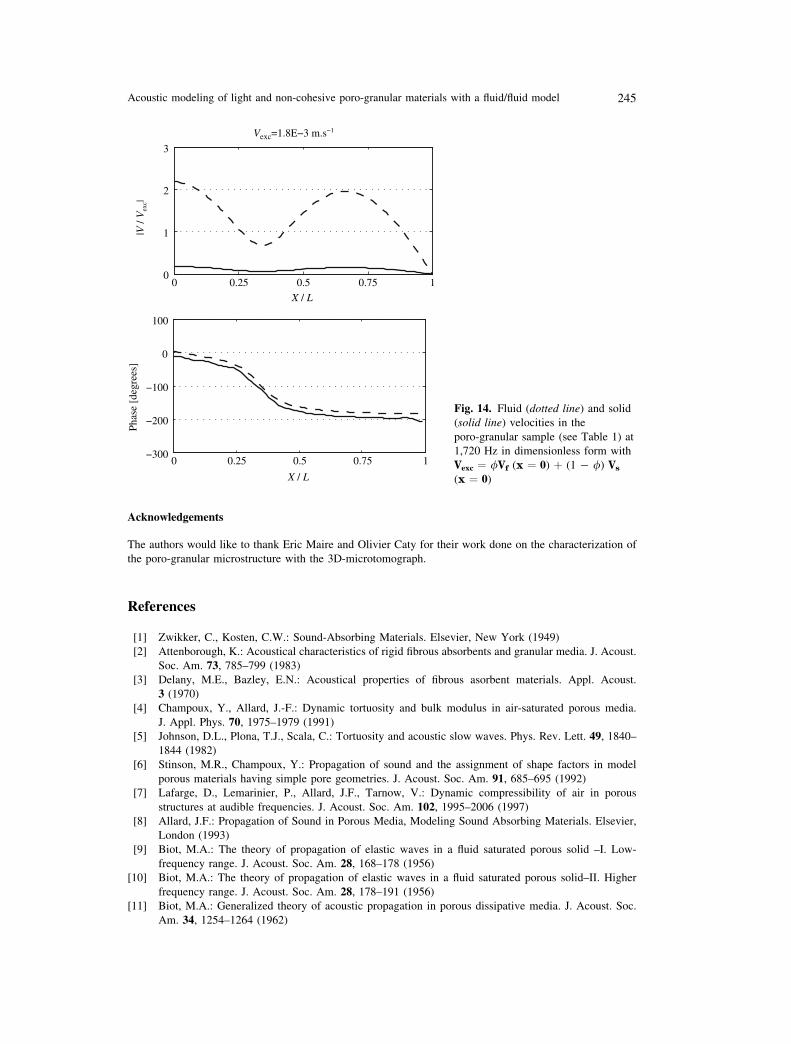
absorption is very low. Finally, Figs. 13 and 14 are related to the second peak of absorption at

1,720 Hz.

At 540 and 1,720 Hz, the magnitude of pressures and velocities in each phase is much higher than

at 1,100 Hz, and explains a better absorption at those frequencies. Moreover, the maximum of

absorption, as expected, occurs when the sample thickness is equal to 1, 3, 5,... quarter wavelength,

while the minimum of absorption occurs when the sample thickness is equal to 2, 4, 6,... quarter

wavelength. In fact, as discussed in the previous Section, viscous dissipations are preponderant in the

studied frequency band. In order to understand the absorption phenomenon, the velocities

distribution is thus necessary, and is more important than the pressures distribution. Indeed, when the

sample thickness is equal to 1, 3, 5,... quarter wavelength, the velocity response is large at x ¼ 0.

Therefore, excitation at those frequencies gives high velocities and leads to high absorption


coefficients. On the contrary, when the sample thickness is equal to 2, 4, 6,... quarter wavelength, the

velocity response is small at x ¼ 0, and the incident wave does not produce high velocity responses.

9 Conclusions

A poro-granular model based on a fluid/fluid description has been presented. The (Ps, Pf) pressure

formulation thus obtained is very simplified compared to classical formulations of Biot’s theory.

Fig. 6. Microstructure of the poro-

granular material obtained by micro-

tomography

500 1000 1500 20000

0.2

0.4

0.6

0.8

1

Frequency [Hz]

Abs

orpt

ion

coef

fici

ent

Fig. 7. Influence of viscous (dottedblack line) and thermal (solid blackline) dissipations on absorption coef-

ficient (grey line) of a 12 cm sample

of poro-granular material (see

Table 1)


Indeed, only two independent variables are necessary to describe the material behavior, instead of

four for the (Us, Pf) formulation of Biot’s model. Moreover, the resolution for the 1D case has

been detailed and used to study thermal and viscous dissipations in solid and fluid phases. This 1D

study is only aimed to present the simplicity of the formulation. Finally, the characterization of a

poro-granular material made of expanded polystyrene granular beads with this model has been

realized, and has proved its reliability and accuracy. The next step of this work will be to apply

this simplified model to a more complex structure with the same simplicity as described in the 1D

case.

0 0.25 0.5 0.75 10

1

2

3

X / L

X / L

|P /

Pex

c|

0 0.25 0.5 0.75 1−100

−50

0

50

Phas

e [d

egre

es]

Fig. 9. Fluid (dotted line) and solid

(solid line) pressures in the

poro-granular sample material (see

Table 1) at 540 Hz in dimensionless

form with Pexc

500 1000 1500 20000

0.2

0.4

0.6

0.8

1

Frequency [Hz]

Abs

orpt

ion

coef

fici

ent

Fig. 8. Influence of fluid (dottedblack line) and solid (solid black line)

dissipations on absorption coefficient

(grey line) of a 12 cm sample of

poro-granular material (see Table 1)


0 0.25 0.5 0.75 10

1

2

3

X / L

X / L

|V /

Vex

c|V

exc=3E−3 m.s−1

0 0.25 0.5 0.75 1−60

−40

−20

0

Phas

e [d

egre

es]


(solid line) velocities in the

poro-granular sample (see Table 1) at

540 Hz in dimensionless form with

Vexc ¼ /Vf (x ¼ 0) þ (1 @ /) Vs

(x ¼ 0)

0 0.25 0.5 0.75 10

0.2

0.4

0.6

0.8

X / L

X / L

|P /

Pex

c|

0 0.25 0.5 0.75 1−200

−150

−100

−50

0

Phas

e [d

egre

es]


(solid line) pressures in the porogran-

ular sample (see Table 1) at 1,100 Hz

in dimensionless form with Pexc


0 0.25 0.5 0.75 10

2

4

6

X / L

X / L

|V /

Vex

c|

Vexc=0.3E−3 m.s−1

0 0.25 0.5 0.75 1−150

−100

−50

0

Phas

e [d

egre

es]



porogranular sample (see Table 1) at

1,100 Hz in dimensionless form with

Vexc ¼ /Vf (x ¼ 0) þ (1 @ /) Vs

(x ¼ 0)

0 0.25 0.5 0.75 10

0.5

1

1.5

X / L

X / L

|P /

Pex

c|

0 0.25 0.5 0.75 1−300

−200

−100

0

100

Phas

e [d

egre

es]


(solid line) pressures in the



Pexc


Acknowledgements

The authors would like to thank Eric Maire and Olivier Caty for their work done on the characterization of

the poro-granular microstructure with the 3D-microtomograph.

References

[1] Zwikker, C., Kosten, C.W.: Sound-Absorbing Materials. Elsevier, New York (1949)

[2] Attenborough, K.: Acoustical characteristics of rigid fibrous absorbents and granular media. J. Acoust.

Soc. Am. 73, 785–799 (1983)

[3] Delany, M.E., Bazley, E.N.: Acoustical properties of fibrous asorbent materials. Appl. Acoust.

3 (1970)

[4] Champoux, Y., Allard, J.-F.: Dynamic tortuosity and bulk modulus in air-saturated porous media.

J. Appl. Phys. 70, 1975–1979 (1991)

[5] Johnson, D.L., Plona, T.J., Scala, C.: Tortuosity and acoustic slow waves. Phys. Rev. Lett. 49, 1840–

1844 (1982)

[6] Stinson, M.R., Champoux, Y.: Propagation of sound and the assignment of shape factors in model

porous materials having simple pore geometries. J. Acoust. Soc. Am. 91, 685–695 (1992)

[7] Lafarge, D., Lemarinier, P., Allard, J.F., Tarnow, V.: Dynamic compressibility of air in porous

structures at audible frequencies. J. Acoust. Soc. Am. 102, 1995–2006 (1997)

[8] Allard, J.F.: Propagation of Sound in Porous Media, Modeling Sound Absorbing Materials. Elsevier,

London (1993)

[9] Biot, M.A.: The theory of propagation of elastic waves in a fluid saturated porous solid –I. Low-

frequency range. J. Acoust. Soc. Am. 28, 168–178 (1956)

[10] Biot, M.A.: The theory of propagation of elastic waves in a fluid saturated porous solid–II. Higher

frequency range. J. Acoust. Soc. Am. 28, 178–191 (1956)

[11] Biot, M.A.: Generalized theory of acoustic propagation in porous dissipative media. J. Acoust. Soc.

Am. 34, 1254–1264 (1962)

0 0.25 0.5 0.75 10

1

2

3

X / L

X / L

|V /

Vex

c| Vexc=1.8E−3 m.s−1

0 0.25 0.5 0.75 1−300

−200

−100

0

100

Phas

e [d

egre

es]





Vexc ¼ /Vf (x ¼ 0) þ (1 @ /) Vs

(x ¼ 0)


[12] Biot, M.A.: The theory of propagation of elastic waves in a fluid saturated porous solid. J. Acoust. Soc.

Am. 28, 168–191 (1956)

[13] Lauriks, W., Boeckx, L., Leclaire, P., Khurana, P., Kelders, L.: Characterisation of porous acoustic

materials. In: SAPEM Proceedings, ENTPE Lyon (2005)

[14] Fellah, Z.E.A., Fellah, M., Sebaa, N., Lauriks, W., Depollier, C.: Measuring flow resistivity of porous

materials at low frequencies range via acoustic transmitted waves (l). J. Acoust. Soc. Am. 119, 1926–

1928 (2006)

[15] Perrot, C., Panneton, R., Olny, X.: Computation of the dynamic bulk modulus of acoustic foams. In:

SAPEM, ENTPE Lyon (2005)

[16] Iannace, G., Ianiello, C., Maffei, L., Romano, R.: Characteristic impedance and complex wave-number

of limestone chips. In: 4th European Conference on Noise Control, Euronoise (2001)

[17] Courtois, T., Falk, T., Bertolini, C.: An acoustical inverse measurement system to determine intrinsic

parameters of porous samples. In: SAPEM, ENTPE Lyon (2005)

[18] Dragonetti, R., Ianniello, C., Romano, R.: The use of an optimization tool to search non-acoustic

parameters of porous materials. Inter-noise, Prague (2004)

[19] Allard, J.F., Depollier, C., Rebillard, P., Lauriks, W., Cops, A.: Inhomogeneous Biot waves in layered

media. J. Appl. Phys. 66, 2278–2284 (1989)

[20] Atalla, N.: An overview of the numerical modeling of poroelastic materials. In: SAPEM, ENTPE Lyon

(2005)

[21] Panneton, R., Atalla, N.: An efficient finite element scheme for solving the three dimensional

poroelasticity problem in acoustics. J. Acoust. Soc. Am. 101, 3287–3298 (1997)

[22] Atalla, N., Panneton, R., Debergue, P.: A mixed displacement–pressure formulation for poroelastic

materials. J. Acoust. Soc. Am. 104, 1444–1452 (1998)

[23] Atalla, N., Hamdi, M.A., Panneton, R.: Enhanced weak integral formulation for the mixed (u, p)

poroelastic equations. J. Acoust. Soc. Am. 109, 3065–3068 (2001)

[24] Debergue, P., Panneton, R., Atalla, N.: Boundary conditions for the weak formulation of the mixed

(u,p) poroelasticity problem. J. Acoust. Soc. Am. 106, 2383–2390 (1999)

[25] Castel, F.: Example of meshing rule for finite element modelling of simple and double porosity

materials. In: SAPEM, ENTPE Lyon (2005)

[26] Dazel, O., Sgard, F., Lamarque, C.-H., Atalla, N.: An extension of complex modes for the resolution of

finite-element poroelastic problems. J. Sound Vib. 253, 421–445 (2002)

[27] Dazel, O., Brouard, B., Depollier, C., Griffiths, S.: An alternative Biot’s displacement formulation for

porous materials. J. Acoust. Soc. Am. 121 (2007)

[28] Hamdi, M.A., Zhang, C., Mebarek, L., Anciant, M., Mahieux, B.: Engineering feedback on numerical

simulation of fully trimmed vehicles using modified biot’s theory. In: SAPEM, ENTPE, Vaulx en

Velin (2005)

[29] Doutres, O., Dauchez, N., Genevaux, J.M., Dazel, O.: Validity of the limp model for porous materials:

A criterion based on the Biot theory. J. Acoust. Soc. Am. 122, 2038–2048 (2007)

[30] Bourinet, J.M.: Approche numerique et experimentale des vibrations amorties de tubes remplis de

materiaux granulaires. These, Ecole Centrale de Nantes (1996)

[31] Bourinet, J.M., Le Houedec, D.: A dynamic stiffness analysis of damped tubes filled with granulars

materials. Comput. Struct. 73, 395–406 (1999)

[32] Saeki, M.: Impact damping with granular materials in a horizontally vibrating system. J. Sound Vib.

251, 153–161 (2002)

[33] Mao, K., Wang, M.Y., Xu, Z., Chen, T.: Simulation and characterization of particle damping in

transient vibrations. American Society of Mechanical Engineers – J. Vib. Acoust. 126 (2004)

[34] Saad, M.H., Adhikari, G., Cardoso, F.: Dem simulation of wave propagation in granular media.

Powder Technol. 109, 222–233 (2000)

[35] Jia, X., Mills, P.: Sound propagation in dense granular materials. Powders and Grains, Kishino (2001)

[36] Voronina, N.N., Horoshenkov, K.V.: A new empirical model for the acoustic properties of loose

granular media. Appl. Acoust. 64, 415–432 (2003)

[37] Attenborough, K.: On the acoustic slow wave in air-filled granular media. J. Acoust. Soc. Am. 81

(1987)

[38] Park, J.: Measurements of the frame acoustic properties of porous and granular materials. J. Acoust.

Soc. Am. 118 (2005)

[39] Horoshenkov, K.V., Swift, M.J.: The acoustic properties of granular materials with pore size

distribution close to log-normal. J. Acoust. Soc. Am. 110, Pt. 1 (2001)


[40] Allard, J.F., Henry, M., Tizianel, J., Kelders, L., Lauriks, W.: Sound propagation in air-saturated

random packings of beads. J. Acoust. Soc. Am. 102, 2004–2007 (1998)

[41] Umnova, O., Attenborough, K., Li, K.M.: Cell model calculations of dynamic drag parameters in

packings of spheres. J. Acoust. Soc. Am. 107 (2000)

[42] Gasser, S., Paun, F., Brechet, Y.: Absorptive properties of rigid porous media: Application to face

centered cubic sphere packing. J. Acoust. Soc. Am. 117, Pt. 1 (2005)

[43] Coste, C., Gilles, B.: On the validity of Hertz contact law for granular material acoustics. Eur. Phys.

J. B 7, 155–168 (1999)

[44] Daniel, R.C., Poloski, A.P., Saez, A.E.: A continuum constitutive model for cohesionless granular

flows. Chem. Engng Sci. 62, 1343–1350 (2007)

[45] Jop, P., Forterre, Y., Pouliquen, O.: A constitutive law for dense granular flows. Nature 441, 727–731

(2006)

[46] Schultz, T., Shaplak, M., Cattafesta, L.N.: Uncertainty analysis of the two microphone method.

J. Sound Vib. 304, 91–109 (2007)

[47] Boden, H., Abom, M.: Influence of errors on the two-microphone method for measuring acoustic

properties in ducts. J. Acoust. Soc. Am. 79, 541–549 (1985)

[48] Seybert, A.F., Soenarko, B.: Error analysis of spectral estimates with application to measurement of

acoustic parameters using random sound fields in ducts. J. Acoust. Soc. Am. 69, 1190–1199 (1981)


Acoustic modeling of light and non-cohesive poro-granular materials...

Documents

Transcript of Acoustic modeling of light and non-cohesive poro-granular materials...