Appendix 3: Additional Control Strategy Information 3a.1 · PDF filepetroleum refineries,...

3a-1

Appendix 3: Additional Control Strategy Information

3a.1 NonEGU Point and Area Source Controls

3a.1.1 NonEGU Point and Area Source Control Strategies for Ozone NAAQS Final

In the NonEGU point and Area Sources portion of the control strategy, maximum control scenarios were used from the existing control measure dataset from AirControlNET 4.1 for 2020 (for geographic areas defined for each level of the standard being analyzed). This existing control measure dataset reflects changes and updates made as a result of the reviews performed for the final PM2.5 RIA. Following this, an internal review was performed by the OAQPS engineers in the Sector Policies and Programs Division (SPPD) to examine the controls applied by AirControlNET and decide if these controls were sufficient or could be more aggressive in their application, given the 2020 analysis year. This review was performed for nonEGU point NOx control measures. The result of this review was an increase in control efficiencies applied for many control measures, and more aggressive control measures for over 70 SCC’s. For example, SPPD recommended that we apply SCR to cement kilns to reduce NOx emissions in 2020. Currently, there are no SCRs in operation at cement kilns in the U.S., but there are several SCRs in operation at cement kilns in France now. Based on the SCR experience at cement kilns in France, SPPD believes SCR could be applied at U.S. cement kilns by 2020. Following this, it was recommended that supplemental controls could be applied to 8 additional SCC’s from nonEGU point NOx sources. We also looked into sources of controls for highly reactive VOC nonEGU point sources. Four additional controls were applied for highly reactive VOC nonEGU point sources not in AirControlNET.

3a.1.2 NOx Control Measures for NonEGU Point Sources.

Several types of NOx control technologies exist for nonEGU point sources: SCR, selective noncatalytic reduction (SNCR), natural gas reburn (NGR), coal reburn, and low-NOx burners. In some cases, LNB accompanied by flue gas recirculation (FGR) is applicable, such as when fuel-borne NOx emissions are expected to be of greater importance than thermal NOx emissions. When circumstances suggest that combustion controls do not make sense as a control technology (e.g., sintering processes, coke oven batteries, sulfur recovery plants), SNCR or SCR may be an appropriate choice. Finally, SCR can be applied along with a combustion control such as LNB with overfire air (OFA) to further reduce NOx emissions. All of these control measures are available for application on industrial boilers.

Besides industrial boilers, other nonEGU point source categories covered in this RIA include petroleum refineries, kraft pulp mills, cement kilns, stationary internal combustion engines, glass manufacturing, combustion turbines, and incinerators. NOx control measures available for petroleum refineries, particularly process heaters at these plants, include LNB, SNCR, FGR, and SCR along with combinations of these technologies. NOx control measures available for kraft pulp mills include those available to industrial boilers, namely LNB, SCR, SNCR, along with water injection (WI). NOx control measures available for cement kilns include those available to industrial boilers, namely LNB, SCR, and SNCR. Non-selective catalytic reduction (NSCR) can be used on stationary internal combustion engines. OXY-firing, a technique to modify

3a-2

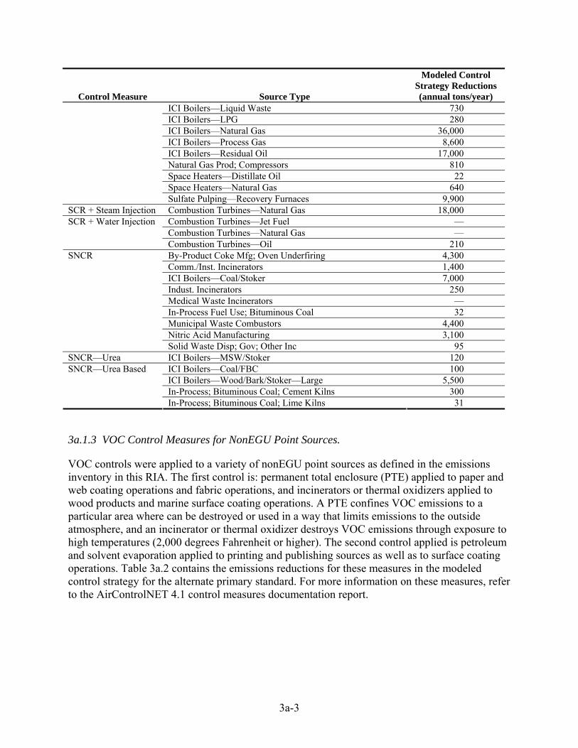
combustion at glass manufacturing plants, can be used to reduce NOx at such plants. LNB, SCR, and SCR + steam injection (SI) are available measures for combustion turbines. Finally, SNCR is an available control technology at incinerators. Table 3a.1 contains a complete list of the NOx nonEGU point control measures applied and their associated emission reductions obtained in the modeled control strategy for the alternate primary standard. For more information on these measures, please refer to the AirControlNET 4.1 control measures documentation report.

Table 3a.1: NOx NonEGU Point Emission Reductions by Control Measure

Control Measure Source Type

Modeled Control Strategy Reductions (annual tons/year)

Biosolid Injection Technology

Cement Kilns 1,200

Asphaltic Conc; Rotary Dryer; Conv Plant 120 Ceramic Clay Mfg; Drying 370 Conv Coating of Prod; Acid Cleaning Bath 440 Fuel Fired Equip; Furnaces; Natural Gas 170 In-Process Fuel Use; Natural Gas 1,300 In-Process Fuel Use; Residual Oil 39 In-Process; Process Gas; Coke Oven Gas 190 Lime Kilns 5,900 Sec Alum Prod; Smelting Furn 62 Steel Foundries; Heat Treating 13

LNB

Surf Coat Oper; Coating Oven Htr; Nat Gas 30 Fluid Cat Cracking Units 3,600 Fuel Fired Equip; Process Htrs; Process Gas 700 In-Process; Process Gas; Coke Oven Gas 880 Iron & Steel Mills—Galvanizing 35 Iron & Steel Mills—Reheating 1,100 Iron Prod; Blast Furn; Blast Htg Stoves 1,000 Sand/Gravel; Dryer 11

LNB + FGR

Steel Prod; Soaking Pits 100 Iron & Steel Mills—Annealing 270 Process Heaters—Distillate Oil 2,300 Process Heaters—Natural Gas 27,000 Process Heaters—Other Fuel 14 Process Heaters—Process Gas 4,200

LNB + SCR

Process Heaters—Residual Oil 37 Rich Burn IC Engines—Gas 22,000 Rich Burn IC Engines—Gas, Diesel, LPG 3,700

NSCR

Rich Burn Internal Combustion Engines—Oil 11,000 Glass Manufacturing—Containers 7,600 Glass Manufacturing—Flat 18,000

OXY-Firing

Glass Manufacturing—Pressed 3,900 Ammonia—NG-Fired Reformers 5,800 Cement Manufacturing—Dry 25,000 Cement Manufacturing—Wet 22,000 IC Engines—Gas 54,000 ICI Boilers—Coal/Cyclone 2,200 ICI Boilers—Coal/Wall 22,000 ICI Boilers—Coke 490

SCR

ICI Boilers—Distillate Oil 4,800

3a-3



ICI Boilers—Liquid Waste 730 ICI Boilers—LPG 280 ICI Boilers—Natural Gas 36,000 ICI Boilers—Process Gas 8,600 ICI Boilers—Residual Oil 17,000 Natural Gas Prod; Compressors 810 Space Heaters—Distillate Oil 22 Space Heaters—Natural Gas 640 Sulfate Pulping—Recovery Furnaces 9,900

SCR + Steam Injection Combustion Turbines—Natural Gas 18,000 Combustion Turbines—Jet Fuel — Combustion Turbines—Natural Gas —

SCR + Water Injection

Combustion Turbines—Oil 210 By-Product Coke Mfg; Oven Underfiring 4,300 Comm./Inst. Incinerators 1,400 ICI Boilers—Coal/Stoker 7,000 Indust. Incinerators 250 Medical Waste Incinerators — In-Process Fuel Use; Bituminous Coal 32 Municipal Waste Combustors 4,400 Nitric Acid Manufacturing 3,100

SNCR

Solid Waste Disp; Gov; Other Inc 95 SNCR—Urea ICI Boilers—MSW/Stoker 120

ICI Boilers—Coal/FBC 100 ICI Boilers—Wood/Bark/Stoker—Large 5,500 In-Process; Bituminous Coal; Cement Kilns 300

SNCR—Urea Based

In-Process; Bituminous Coal; Lime Kilns 31

3a.1.3 VOC Control Measures for NonEGU Point Sources.

VOC controls were applied to a variety of nonEGU point sources as defined in the emissions inventory in this RIA. The first control is: permanent total enclosure (PTE) applied to paper and web coating operations and fabric operations, and incinerators or thermal oxidizers applied to wood products and marine surface coating operations. A PTE confines VOC emissions to a particular area where can be destroyed or used in a way that limits emissions to the outside atmosphere, and an incinerator or thermal oxidizer destroys VOC emissions through exposure to high temperatures (2,000 degrees Fahrenheit or higher). The second control applied is petroleum and solvent evaporation applied to printing and publishing sources as well as to surface coating operations. Table 3a.2 contains the emissions reductions for these measures in the modeled control strategy for the alternate primary standard. For more information on these measures, refer to the AirControlNET 4.1 control measures documentation report.

3a-4

Table 3a.2: VOC NonEGU Point Emission Reductions by Control Measure



Fabric Printing, Coating and Dyeing 43 Permanent Total Enclosure (PTE) Paper and Other Web Coating 490 Printing and Publishing 3,600 Petroleum and Solvent Evaporation Surface Coating 400

3a.1.4 NOx Control Measures for Area Sources

There were three control measures applied for NOx emissions from area sources. The first is RACT (reasonably available control technology) to 25 tpy (LNB). This control is the addition of a low NOx burner to reduce NOx emissions. This control is applied to industrial oil, natural gas, and coal combustion sources. The second control is water heaters plus LNB space heaters. This control is based on the installation of low-NOx space heaters and water heaters in commercial and institutional sources for the reduction of NOx emissions. The third control was switching to low sulfur fuel for residential home heating. This control is primarily designed to reduce sulfur dioxide, but has a co-benefit of reducing NOx. Table 3a.3 contains the listing of control measures and associated reductions for the modeled control strategy. For additional information regarding these controls please refer to the AirControlNET 4.1 control measures documentation report.

Table 3a.3: NOx Area Source Emission Reductions by Control Measure


Modeled Control Strategy Reductions

(annual tons/year) Industrial Coal Combustion 5,400 Industrial NG Combustion 3,000

RACT to 25 tpy (LNB)

Industrial Oil Combustion 570 Switch to Low Sulfur Fuel Residential Home Heating 970

Commercial/Institutional—NG 4,300 Water Heater + LNB Space Heaters Residential NG 6,700

3a.1.5 VOC Control Measures for Area Source.

The most frequently applied control to reduce VOC emissions from area sources was CARB Long-Term Limits. This control, which represents controls available in VOC rules promulgated by the California Air Resources Board, applies to commercial solvents and commercial adhesives, and depends on future technological innovation and market incentive methods to achieve emission reductions. The next most frequently applied control was the use of low or no VOC materials for graphic art source categories. The South Coast Air District’s SCAQMD Rule 1168 control applies to wood furniture and solvent source categories sets limits for adhesive and sealant VOC content. The OTC solvent cleaning rule control establishes hardware and operating requirements for specified vapor cleaning machines, as well as solvent volatility limits and operating practices for cold cleaners. The Low Pressure/Vacuum Relief Valve control measure is the addition of low pressure/vacuum (LP/V) relief valves to gasoline storage tanks at service

3a-5

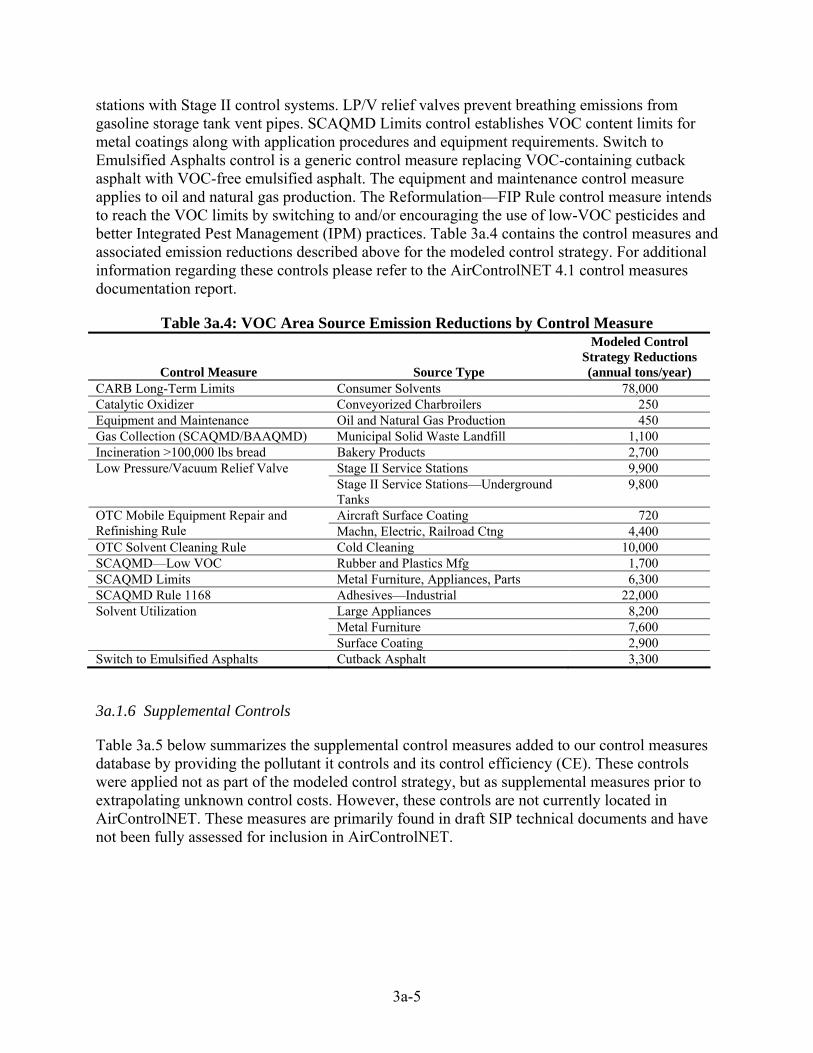
stations with Stage II control systems. LP/V relief valves prevent breathing emissions from gasoline storage tank vent pipes. SCAQMD Limits control establishes VOC content limits for metal coatings along with application procedures and equipment requirements. Switch to Emulsified Asphalts control is a generic control measure replacing VOC-containing cutback asphalt with VOC-free emulsified asphalt. The equipment and maintenance control measure applies to oil and natural gas production. The Reformulation—FIP Rule control measure intends to reach the VOC limits by switching to and/or encouraging the use of low-VOC pesticides and better Integrated Pest Management (IPM) practices. Table 3a.4 contains the control measures and associated emission reductions described above for the modeled control strategy. For additional information regarding these controls please refer to the AirControlNET 4.1 control measures documentation report.

Table 3a.4: VOC Area Source Emission Reductions by Control Measure



CARB Long-Term Limits Consumer Solvents 78,000 Catalytic Oxidizer Conveyorized Charbroilers 250 Equipment and Maintenance Oil and Natural Gas Production 450 Gas Collection (SCAQMD/BAAQMD) Municipal Solid Waste Landfill 1,100 Incineration >100,000 lbs bread Bakery Products 2,700

Stage II Service Stations 9,900 Low Pressure/Vacuum Relief Valve Stage II Service Stations—Underground Tanks

9,800

Aircraft Surface Coating 720 OTC Mobile Equipment Repair and Refinishing Rule Machn, Electric, Railroad Ctng 4,400 OTC Solvent Cleaning Rule Cold Cleaning 10,000 SCAQMD—Low VOC Rubber and Plastics Mfg 1,700 SCAQMD Limits Metal Furniture, Appliances, Parts 6,300 SCAQMD Rule 1168 Adhesives—Industrial 22,000

Large Appliances 8,200 Metal Furniture 7,600

Solvent Utilization

Surface Coating 2,900 Switch to Emulsified Asphalts Cutback Asphalt 3,300

3a.1.6 Supplemental Controls

Table 3a.5 below summarizes the supplemental control measures added to our control measures database by providing the pollutant it controls and its control efficiency (CE). These controls were applied not as part of the modeled control strategy, but as supplemental measures prior to extrapolating unknown control costs. However, these controls are not currently located in AirControlNET. These measures are primarily found in draft SIP technical documents and have not been fully assessed for inclusion in AirControlNET.

3a-6

Table 3a.5: Supplemental Emissions Control Measures Added to the Control Measures Database

Poll Control

Technology SCC SCC

Description

Percent Reduction

(%) 20200252 Internal Comb. Engines/Industrial/

Natural Gas/2-cycle Lean Burn 87 NOx LEC

20200254 Internal Comb. Engines/Industrial/ Natural Gas/4-cycle Lean Burn

87

3018001- Fugitive Leaks 50 Enhanced LDAR 30600701 30600999 -

Flares 98

LDAR 3018001 - Fugitive Leaks 80 Monitoring Program 30600702- Cooling towers No general

estimate Inspection and Maintenance Program (Separators) Water Seals (Drains)

30600503- Wastewater Drains and Separators 65

Work Practices, Use of Low VOC Coatings (Area Sources)

2401025000 2401030000 2401060000 2425010000 2425030000 2425040000 2461050000

Solvent Utilization 90

VOC

Work Practices, Use of Low VOC Coatings (NonEGU Point)

307001199 Surface Coating Operations within SCC 4020000000, Printing/Publishing processes within SCC 4050000000

Petroleum and Solvent Evaporation 90

Low Emission Combustion (LEC)

Overview: LEC technology is defined as the modification of a natural gas fueled, spark ignited, reciprocating internal combustion engine to reduce emissions of NOx by utilizing ultra-lean air-fuel ratios, high energy ignition systems and/or pre-combustion chambers, increased turbocharging or adding a turbocharger, and increased cooling and/or adding an intercooler or aftercooler, resulting in an engine that is designed to achieve a consistent NOx emission rate of not more than 1.5-3.0 g/bhp-hr at full capacity (usually 100 percent speed and 100 percent load). This type of retrofit technology is fairly widely available for stationary internal combustion engines.

For CE, EPA estimates that it ranges from 82 to 91 percent for LEC technology applications. The EPA believes application of LEC would achieve average NOx emission levels in the range of 1.5-3.0 g/bhp-hr. This is an 82-91 percent reduction from the average uncontrolled emission levels reported in the ACT document. An EPA memorandum summarizing 269 tests shows that

3a-7

96 percent of IC engines with installed LEC technology achieved emission rates of less than 2.0 g/bhp-hr.1 The 2000 EC/R report on IC engines summarizes 476 tests and shows that 97% of the IC engines with installed LEC technology achieve emission rates of 2.0 g/bhp-hr or less.2

Major Uncertainties: The EPA acknowledges that specific values will vary from engine to engine. The amount of control desired and number of operating hours will make a difference in terms of the impact had from a LEC retrofit. Also, the use of LEC may yield improved fuel economy and power output, both of which may affect the emissions generated by the device.

Leak Detection and Repair (LDAR) for Fugitive Leaks

Overview: This control measure is a program to reduce leaks of fugitive VOC emissions from chemical plants and refineries. The program includes special “sniffer” equipment to detect leaks, and maintenance schedules that affected facilities are to adhere to. This program is one that is contained within the Houston-Galveston-Brazoria 8-hour Ozone SIP.

Major Uncertainties: The degree of leakage from pipes and processes at chemical plants is always difficult to quantify given the large number of such leaks at a typical chemical manufacturing plant. There are also growing indications based on tests conducted by TCEQ and others in Harris County, Texas that fugitive leaks have been underestimated from chemical plants by a factor of 6 to 20 or greater. 3

Enhanced LDAR for Fugitive Leaks

Overview: This control measure is a more stringent program to reduce leaks of fugitive VOC emissions from chemical plants and refineries that presumes that an existing LDAR program already is in operation.

Major Uncertainties: The calculations of CE and cost presume use of LDAR at a chemical plant. This should not be an unreasonable assumption, however, given that most chemical plants are under some type of requirement to have an LDAR program. However, as mentioned earlier, there is growing evidence that fugitive leak emissions are underestimated from chemical plants by a factor of 6 to 20 or greater.4

1 “Stationary Reciprocating Internal Combustion Engines Technical Support Document for NOx SIP Call Proposal,” U.S. Environmental Protection Agency. September 5, 2000. Available on the Internet at http://www.epa.gov/ttn/naaqs/ozone/rto/sip/data/tsd9-00.pdf. 2“Stationary Internal Combustion Engines: Updated Information on NOx Emissions and Control Techniques,” Ec/R Incorporated, Chapel Hill, NC. September 1, 2000. Available on the Internet at http://www.epa.gov/ttn/naaqs/ozone/ozonetech/ic_engine_nox_update_09012000.pdf. 3 VOC Fugitive Losses: New Monitors, Emissions Losses, and Potential Policy Gaps. 2006 International Workshop. U.S. Environmental Protection Agency, Office of Air Quality Planning and Standards and Office of Solid Waste and Emergency Response. October 25-27, 2006. 4 VOC Fugitive Losses: New Monitors, Emissions Losses, and Potential Policy Gaps. 2006 International Workshop. U.S. Environmental Protection Agency, Office of Air Quality Planning and Standards and Office of Solid Waste and Emergency Response. October 25-27, 2006.

3a-8

Flare Gas Recovery

Overview: This control measure is a condenser that can recover 98 percent of the VOC emitted by flares that emit 20 tons per year or more of the pollutant.

Major Uncertainties: Flare gas recovery is just gaining commercial acceptance in the US and is only in use at a small number of refineries.

Cooling Towers

Overview: The control measure is continuous monitoring of VOC from the cooling water return to a level of 10 ppb. This monitoring is accomplished by using a continuous flow monitor at the inlet to each cooling tower.

There is not a general estimate of CE for this measure; one is to apply a continuous flow monitor until VOC emissions have reached a level of 1.7 tons/year for a given cooling tower.5

Major Uncertainties: The amount of VOC leakage from each cooling tower can greatly affect the overall cost-effectiveness of this control measure.

Wastewater Drains and Separators

Overview: This control measure includes an inspection and maintenance program to reduce VOC emissions from wastewater drains and water seals on drains. This measure is a more stringent version of measures that underlie existing NESHAP requirements for such sources.

Major Uncertainties: The reference for this control measures notes that the VOC emissions inventories for the five San Francisco Bay Area refineries whose data was a centerpiece of this report are incomplete. In addition, not all VOC species from these sources were included in the VOC data that is a basis for these calculations.6

Work Practices or Use of Low VOC Coatings

Overview: The control measure is either application of work practices (e.g., storing VOC-containing cleaning materials in closed containers, minimizing spills) or using coatings that have much lower VOC content. These measures, which are of relatively low cost compared to other VOC area source controls, can apply to a variety of processes, both for non-EGU point and area sources, in different industries and is defined in the proposed control techniques guidelines (CTG) for paper, film and foil coatings, metal furniture coatings, and large appliance coatings published by the US EPA in July 2007.7

5 Bay Area Air Quality Management District (BAAQMD). Proposed Revision of Regulation 8, Rule 8: Wastewater Collection Systems. Staff Report, March 17, 2004. 6 Bay Area Air Quality Management District (BAAQMD). Proposed Revision of Regulation 8, Rule 8: Wastewater Collection Systems. Staff Report, March 17, 2004. 7 U.S. Environmental Protection Agency. Consumer and Commercial Products: Control Techniques Guidelines in Lieu of Regulations for Paper, Film, and Foil Coatings; Metal

3a-9

The estimated CE expected to be achieved by either of these control measures is 90 percent.

Major Uncertainties: The greatest uncertainty is in how many potentially affected processes are implementing or already implemented these control measures. This may be particularly true in California. Also, there are nine States that have many of the above work practices in effect for paper, film and foil coatings processes, but the work practices are not meant to achieve a specific emissions limit.8 Hence, it is uncertain how much VOC reduction is occurring from this control measure in this case.

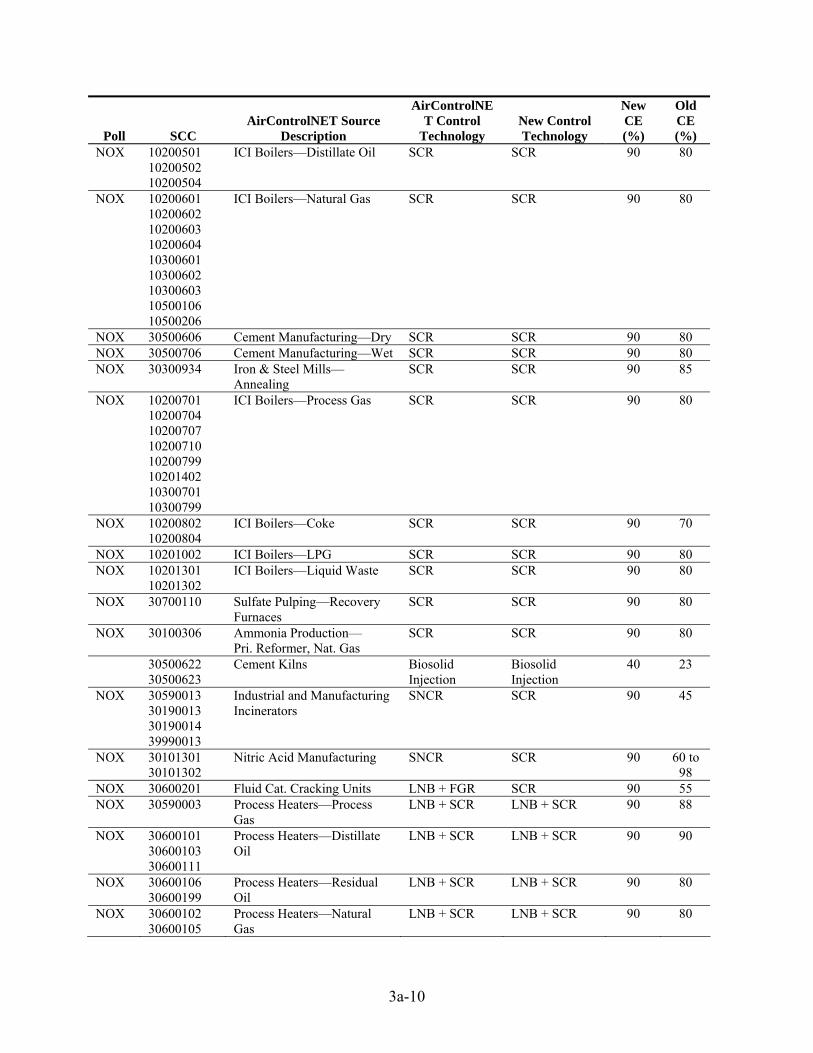
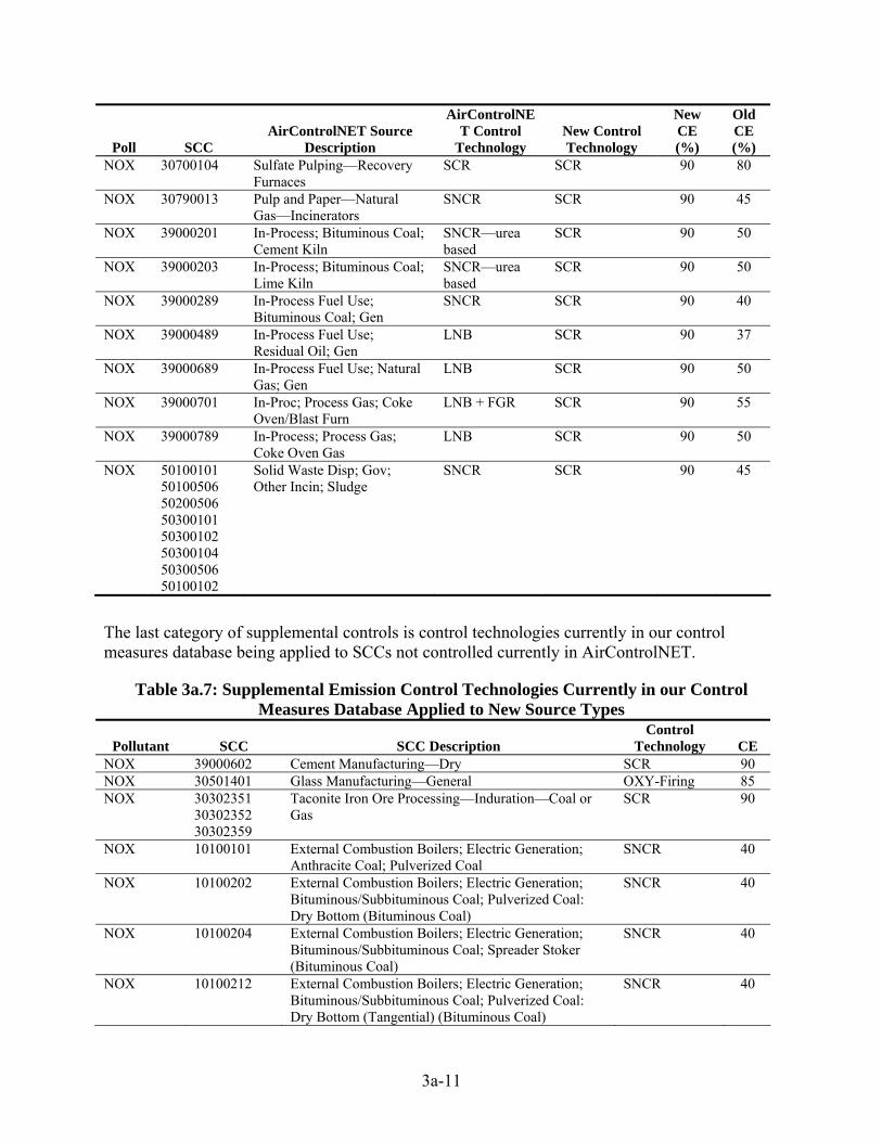
In addition to the new supplemental controls presented above, there were a number of changes made to existing AirControlNET controls. These changes were made based upon an internal review performed by EPA engineers to examine the controls applied by AirControlNET and determine if these controls were sufficient or could be more aggressive in their application, given the 2020 analysis year. This review was performed for nonEGU point NOx control measures. The result of this review was an increase in control efficiencies applied for many control measures, and more aggressive control measures for over 70 SCCs. The changes apply to the control strategies performed for the Eastern US only. These changes are listed in Table 3a.6.

Table 3a.6: Supplemental Emission Control Measures—Changes to Control Technologies Currently in our Control Measures Database For Application in 2020

Poll SCC AirControlNET Source

Description

AirControlNET Control

Technology New Control Technology

New CE (%)

Old CE (%)

NOX 10200104 10200204 10200205 10300207 10300209 10200217 10300216

ICI Boilers—Coal-Stoker SNCR SCR 90 40

NOX 10200901 10200902 10200903 10200907 10300902 10300903

ICI Boilers—Wood/Bark/ Waste

SNCR SCR 90 55

NOX 10200401 10200402 10200404 10200405 10300401

ICI Boilers—Residual Oil SCR SCR 90 80

Furniture Coatings; and Large Appliance Coatings. 40 CFR 59. July 10, 2007. Available on the Intenet at http://www.epa.gov/ttncaaa1/t1/fr_notices/ctg_ccp092807.pdf. It should be noted that this CTG became final in October 2007. 8 U.S. Environmental Protection Agency. Consumer and Commercial Products: Control Techniques Guidelines in Lieu of Regulations for Paper, Film, and Foil Coatings; Metal Furniture Coatings; and Large Appliance Coatings. 40 CFR 59. July 10, 2007, p. 37597. Available on the Intenet at http://www.epa.gov/ttncaaa1/t1/fr_notices/ctg_ccp092807.pdf.

3a-10


Description



New CE (%)

Old CE (%)

NOX 10200501 10200502 10200504

ICI Boilers—Distillate Oil SCR SCR 90 80

NOX 10200601 10200602 10200603 10200604 10300601 10300602 10300603 10500106 10500206

ICI Boilers—Natural Gas SCR SCR 90 80

NOX 30500606 Cement Manufacturing—Dry SCR SCR 90 80 NOX 30500706 Cement Manufacturing—Wet SCR SCR 90 80 NOX 30300934 Iron & Steel Mills—

Annealing SCR SCR 90 85

NOX 10200701 10200704 10200707 10200710 10200799 10201402 10300701 10300799

ICI Boilers—Process Gas SCR SCR 90 80

NOX 10200802 10200804

ICI Boilers—Coke SCR SCR 90 70

NOX 10201002 ICI Boilers—LPG SCR SCR 90 80 NOX 10201301

10201302 ICI Boilers—Liquid Waste SCR SCR 90 80

NOX 30700110 Sulfate Pulping—Recovery Furnaces

SCR SCR 90 80

NOX 30100306 Ammonia Production— Pri. Reformer, Nat. Gas

SCR SCR 90 80

30500622 30500623

Cement Kilns Biosolid Injection

Biosolid Injection

40 23

NOX 30590013 30190013 30190014 39990013

Industrial and Manufacturing Incinerators

SNCR SCR 90 45

NOX 30101301 30101302

Nitric Acid Manufacturing SNCR SCR 90 60 to 98

NOX 30600201 Fluid Cat. Cracking Units LNB + FGR SCR 90 55 NOX 30590003 Process Heaters—Process

Gas LNB + SCR LNB + SCR 90 88

NOX 30600101 30600103 30600111

Process Heaters—Distillate Oil

LNB + SCR LNB + SCR 90 90

NOX 30600106 30600199

Process Heaters—Residual Oil


NOX 30600102 30600105

Process Heaters—Natural Gas


3a-11


Description



New CE (%)

Old CE (%)

NOX 30700104 Sulfate Pulping—Recovery Furnaces

SCR SCR 90 80

NOX 30790013 Pulp and Paper—Natural Gas—Incinerators

SNCR SCR 90 45

NOX 39000201 In-Process; Bituminous Coal; Cement Kiln

SNCR—urea based

SCR 90 50

NOX 39000203 In-Process; Bituminous Coal; Lime Kiln

SNCR—urea based

SCR 90 50

NOX 39000289 In-Process Fuel Use; Bituminous Coal; Gen

SNCR SCR 90 40

NOX 39000489 In-Process Fuel Use; Residual Oil; Gen

LNB SCR 90 37

NOX 39000689 In-Process Fuel Use; Natural Gas; Gen

LNB SCR 90 50

NOX 39000701 In-Proc; Process Gas; Coke Oven/Blast Furn

LNB + FGR SCR 90 55

NOX 39000789 In-Process; Process Gas; Coke Oven Gas

LNB SCR 90 50

NOX 50100101 50100506 50200506 50300101 50300102 50300104 50300506 50100102

Solid Waste Disp; Gov; Other Incin; Sludge

SNCR SCR 90 45

The last category of supplemental controls is control technologies currently in our control measures database being applied to SCCs not controlled currently in AirControlNET.

Table 3a.7: Supplemental Emission Control Technologies Currently in our Control Measures Database Applied to New Source Types

Pollutant SCC SCC Description Control

Technology CE NOX 39000602 Cement Manufacturing—Dry SCR 90 NOX 30501401 Glass Manufacturing—General OXY-Firing 85 NOX 30302351

30302352 30302359

Taconite Iron Ore Processing—Induration—Coal or Gas

SCR 90

NOX 10100101 External Combustion Boilers; Electric Generation; Anthracite Coal; Pulverized Coal

SNCR 40

NOX 10100202 External Combustion Boilers; Electric Generation; Bituminous/Subbituminous Coal; Pulverized Coal: Dry Bottom (Bituminous Coal)

SNCR 40

NOX 10100204 External Combustion Boilers; Electric Generation; Bituminous/Subbituminous Coal; Spreader Stoker (Bituminous Coal)

SNCR 40

NOX 10100212 External Combustion Boilers; Electric Generation; Bituminous/Subbituminous Coal; Pulverized Coal: Dry Bottom (Tangential) (Bituminous Coal)

SNCR 40

3a-12

Pollutant SCC SCC Description Control

Technology CE NOX 10100401 External Combustion Boilers; Electric Generation;

Residual Oil; Grade 6 Oil: Normal Firing SNCR 50

NOX 10100404 External Combustion Boilers; Electric Generation; Residual Oil; Grade 6 Oil: Tangential Firing

SNCR 50

NOX 10100501 External Combustion Boilers; Electric Generation; Distillate Oil; Grades 1 and 2 Oil

SNCR 50

NOX 10100601 External Combustion Boilers; Electric Generation; Natural Gas; Boilers > 100 Million Btu/hr except Tangential

NGR 50

NOX 10100602 External Combustion Boilers; Electric Generation; Natural Gas; Boilers < 100 Million Btu/hr except Tangential

NGR 50

NOX 10100604 External Combustion Boilers; Electric Generation; Natural Gas; Tangentially Fired Units

NGR 50

NOX 10101202 External Combustion Boilers; Electric Generation; Solid Waste; Refuse Derived Fuel

SNCR 50

NOX 20200253 Internal Comb. Engines/Industrial/Natural Gas/4-cycle Rich Burn

NSCR 90

3a.2 Mobile Control Measures Used in Control Scenarios

Tables 3a.8 and 3a.9 summarize the emission reductions for the mobile source control measures discussed in this section.

Table 3a.8: NOx Mobile Emission Reductions by Control Measure

Sector Control Measure Modeled Control Strategy Reductions

(annual tons/year) Eliminate Long Duration Truck Idling 5,800 Reduce Gasoline RVP 880 Diesel Retrofits 91,000 Continuous Inspection and Maintenance 20,000

Onroad

Commuter Programs 4,100 Nonroad Diesel Retrofits and Engine Rebuilds 35,000

Table 3a.9: VOC Mobile Emission Reductions by Control Measure

Sector Control Measure Modeled Control Strategy Reductions

(annual tons/year) Reduce Gasoline RVP 17,000 Diesel Retrofits 8,400 Continuous Inspection and Maintenance 28,000

Onroad

Commuter Programs 7,000 Reduce Gasoline RVP 6,300 Nonroad Diesel Retrofits and Engine Rebuilds 5,200

3a-13

3a.2.1 Diesel Retrofits and Engine Rebuilds

Retrofitting heavy-duty diesel vehicles and equipment manufactured before stricter standards are in place—in 2007–2010 for highway engines and in 2011–2014 for most nonroad equipment—can provide NOX and HC benefits. The retrofit strategies included in the RIA retrofit measure are:

• Installation of emissions after-treatment devices called selective catalytic reduction (“SCRs”)

• Rebuilding nonroad engines (“rebuild/upgrade kit”)

We chose to focus on these strategies due to their high NOx emissions reduction potential and widespread application. Additional retrofit strategies include, but are not limited to, lean NOx catalyst systems—which are another type of after-treatment device—and alternative fuels. Additionally, SCRs are currently the most likely type of control technology to be used to meet EPA’s NOx 2007–2010 requirements for HD diesel trucks and 2008–2011 requirements for nonroad equipment. Actual emissions reductions may vary significantly by strategy and by the type and age of the engine and its application.

To estimate the potential emissions reductions from this measure, we applied a mix of two retrofit strategies (SCRs and rebuild/upgrade kits) for the 2020 inventory of:

• Heavy-duty highway trucks class 6 & above, Model Year 1995–2009

• All diesel nonroad engines, Model Year 1991–2007, except for locomotive, marine, pleasure craft, & aircraft engines

Class 6 and above trucks comprise the bulk of the NOx emissions inventory from heavy-duty highway vehicles, so we did not include trucks below class 6. We chose not to include locomotive and marine engines in our analysis since EPA has proposed regulations to address these engines, which will significantly impact the emissions inventory and emission reduction potential from retrofits in 2020. There was also not enough data available to assess retrofit strategies for existing aircraft and pleasure craft engines, so we did not include them in this analysis. In addition, EPA is in the process of negotiating standards for new aircraft engines.

The lower bound in the model year range—1995 for highway vehicles and 1991 for nonroad engines—reflects the first model year in which emissions after-treatment devices can be reliably applied to the engines. Due to a variety of factors, devices are at a higher risk of failure for earlier model years. We expect the engines manufactured before the lower bound year that are still in existence in 2020 to be retired quickly due to natural turnover, therefore, we have not included strategies for pre-1995/1991 engines because of the strategies’ relatively small impact on emissions. The upper bound in the model year range reflects the last year before more stringent emissions standards will be fully phased-in.

We chose the type of strategy to apply to each model year of highway vehicles and nonroad equipment based on our technical assessment of which strategies would achieve reliable results at the lowest cost. After-treatment devices can be more cost-effective than rebuild and vice versa

3a-14

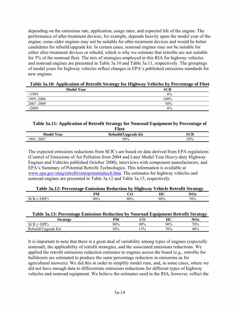
depending on the emissions rate, application, usage rates, and expected life of the engine. The performance of after-treatment devices, for example, depends heavily upon the model year of the engine; some older engines may not be suitable for after-treatment devices and would be better candidates for rebuild/upgrade kit. In certain cases, nonroad engines may not be suitable for either after-treatment devices or rebuild, which is why we estimate that retrofits are not suitable for 5% of the nonroad fleet. The mix of strategies employed in this RIA for highway vehicles and nonroad engines are presented in Table 3a.10 and Table 3a.11, respectively. The groupings of model years for highway vehicles reflect changes in EPA’s published emissions standards for new engines.

Table 3a.10: Application of Retrofit Strategy for Highway Vehicles by Percentage of Fleet Model Year SCR

<1995 0% 1995–2006 100% 2007–2009 50% >2009 0%

Table 3a.11: Application of Retrofit Strategy for Nonroad Equipment by Percentage of Fleet

Model Year Rebuild/Upgrade kit SCR 1991–2007 50% 50%

The expected emissions reductions from SCR’s are based on data derived from EPA regulations (Control of Emissions of Air Pollution from 2004 and Later Model Year Heavy-duty Highway Engines and Vehicles published October 2000), interviews with component manufacturers, and EPA’s Summary of Potential Retrofit Technologies. This information is available at www.epa.gov/otaq/retrofit/retropotentialtech.htm. The estimates for highway vehicles and nonroad engines are presented in Table 3a.12 and Table 3a.13, respectively.

Table 3a.12: Percentage Emissions Reduction by Highway Vehicle Retrofit Strategy PM CO HC NOx

SCR (+DPF) 90% 90% 90% 70%

Table 3a.13: Percentage Emissions Reduction by Nonroad Equipment Retrofit Strategy Strategy PM CO HC NOx

SCR (+DPF) 90% 90% 90% 70% Rebuild/Upgrade Kit 30% 15% 70% 40%

It is important to note that there is a great deal of variability among types of engines (especially nonroad), the applicability of retrofit strategies, and the associated emissions reductions. We applied the retrofit emissions reduction estimates to engines across the board (e.g., retrofits for bulldozers are estimated to produce the same percentage reduction in emissions as for agricultural mowers). We did this in order to simplify model runs, and, in some cases, where we did not have enough data to differentiate emissions reductions for different types of highway vehicles and nonroad equipment. We believe the estimates used in the RIA, however, reflect the

3a-15

best available estimates of emissions reductions that can be expected from retrofitting the heavy-duty diesel fleet.

Using the retrofit module in EPA’s National Mobile Inventory Model (NMIM) available at http://www.epa.gov/otaq/nmim.htm, we calculated the total percentage reduction in emissions (PM, NOx, HC, and CO) from the retrofit measure for each relevant engine category (source category code, or SCC) for each county in 2020. To evaluate this change in the emissions inventory, we conducted both a baseline and control analysis. Both analyses were based on NMIM 2005 (version NMIM20060310), NONROAD2005 (February 2006), and MOBILE6.2.03 which included the updated diesel PM file PMDZML.csv dated March 17, 2006.

For the control analysis, we applied the retrofit measure corresponding to the percent reductions of the specified pollutants in Tables 3a.12 and 3a.13 to the specified model years in Tables 3a.10 and 3a.11 of the relevant SCCs. Fleet turnover rates are modeled in the NMIM, so we applied the retrofit measure to the 2007 fleet inventory, and then evaluated the resulting emissions inventory in 2020. The timing of the application of the retrofit measure is not a factor; retrofits only need to take place prior to the attainment date target (2020 for this RIA). For example, if retrofit devices are installed on 1995 model year bulldozers in 2007, the only impact on emissions in 2020 will be from the expected inventory of 1995 model year bulldozer emissions in 2020.

We then compared the baseline and control analyses to determine the percent reduction in emissions we estimate from this measure for the relevant SCC codes in the targeted nonattainment areas.

3a.2.2 Implement Continuous Inspection and Maintenance Using Remote Onboard Diagnostics (OBD)

Continuous Inspection and Maintenance (I/M) is a new way to check the status of OBD systems on light-duty OBD-equipped vehicles. It involves equipping subject vehicles with some type of transmitter that attaches to the OBD port. The device transmits the status of the OBD system to receivers distributed around the I/M area. Transmission may be through radio-frequency, cellular or wi-fi means. Radio frequency and cellular technologies are currently being used in the states of Oregon, California and Maryland.

Current I/M programs test light-duty vehicles on a periodic basis—either annually or biennially. Emission reduction credit is assigned based on test frequency. Using Continuous I/M, vehicles are continuously monitored as they are operated throughout the non-attainment area. When a vehicle experiences an OBD failure, the motorist is notified and is required to get repairs within the normal grace period—typically about a month. Thus, Continuous I/M will result in repairs happening essentially whenever a malfunction occurs that would cause the check engine light to illuminate. The continuous I/M program is applied to the same fleet of vehicles as the current periodic I/M programs. Currently, MOBILE6 provides an increment of benefit when going from a biennial program to an annual program. The same increment of credit applies going from an annual program to a continuous program.

Source Categories Affected by Measure:

3a-16

• All 1996 and newer light-duty gasoline vehicles and trucks:

• All 1996 and newer (SCC 2201001000) Light Duty Gasoline Vehicles (LDGV), Total: All Road Types

• All 1996 and newer (SCC 2201020000) Light Duty Gasoline Trucks 1 (LDGT1), Total: All Road Types

• All 1996 and newer (SCC 2201040000) Light Duty Gasoline Trucks 2 (LDGT2), Total: All Road Types

OBD systems on light duty vehicles are required to illuminate the malfunction indicator lamp whenever emissions of HC, CO or NOx would exceed 1.5 times the vehicle’s certification standard. Thus, the benefits of this measure will affect all three criteria pollutants. MOBILE6 was used to estimate the emission reduction benefits of Continuous I/M, using the methodology discussed above.

3a.2.3 Eliminating Long Duration Truck Idling

Virtually all long duration truck idling—idling that lasts for longer than 15 minutes—from heavy-duty diesel class 8a and 8b trucks can be eliminated with two strategies:

• truck stop & terminal electrification (TSE)

• mobile idle reduction technologies (MIRTs) such as auxiliary power units, generator sets, and direct-fired heaters

TSE can eliminate idling when trucks are resting at truck stops or public rest areas and while trucks are waiting to perform a task at private distribution terminals. When truck spaces are electrified, truck drivers can shut down their engines and use electricity to power equipment which supplies air conditioning, heat, and electrical power for on-board appliances.

MIRTs can eliminate long duration idling from trucks that are stopped away from these central sites. For a more complete list of MIRTs see EPA’s Idle Reduction Technology page at http://www.epa.gov/otaq/smartway/idlingtechnologies.htm.

This measure demonstrates the potential emissions reductions if every class 8a and 8b truck is equipped with a MIRT or has dependable access to sites with TSE in 2020.

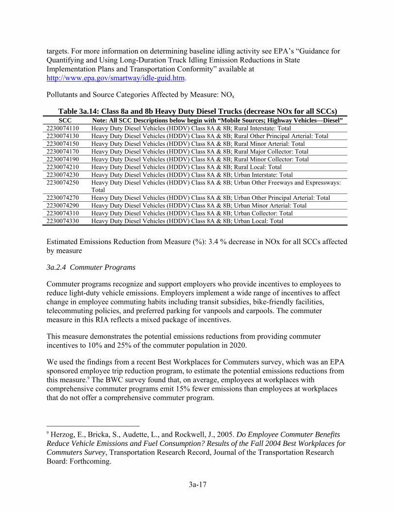
To estimate the potential emissions reduction from this measure, we applied a reduction equal to the full amount of the emissions attributed to long duration idling in the MOBILE model, which is estimated to be 3.4% of the total NOx emissions from class 8a and 8b heavy duty diesel trucks. Since the MOBILE model does not distinguish between idling and operating emissions, EPA estimates idling emissions in the inventory based on fuel conversion factors. The inventory in the MOBILE model, however, does not fully capture long duration idling emissions. There is evidence that idling may represent a much greater share than 3.4% of the real world inventory, based on engine control module data from long haul trucking companies. As such, we believe the emissions reductions demonstrated from this measure in the RIA represent ambitious but realistic

3a-17

targets. For more information on determining baseline idling activity see EPA’s “Guidance for Quantifying and Using Long-Duration Truck Idling Emission Reductions in State Implementation Plans and Transportation Conformity” available at http://www.epa.gov/smartway/idle-guid.htm.

Pollutants and Source Categories Affected by Measure: NOx

Table 3a.14: Class 8a and 8b Heavy Duty Diesel Trucks (decrease NOx for all SCCs) SCC Note: All SCC Descriptions below begin with “Mobile Sources; Highway Vehicles—Diesel”

2230074110 Heavy Duty Diesel Vehicles (HDDV) Class 8A & 8B; Rural Interstate: Total 2230074130 Heavy Duty Diesel Vehicles (HDDV) Class 8A & 8B; Rural Other Principal Arterial: Total 2230074150 Heavy Duty Diesel Vehicles (HDDV) Class 8A & 8B; Rural Minor Arterial: Total 2230074170 Heavy Duty Diesel Vehicles (HDDV) Class 8A & 8B; Rural Major Collector: Total 2230074190 Heavy Duty Diesel Vehicles (HDDV) Class 8A & 8B; Rural Minor Collector: Total 2230074210 Heavy Duty Diesel Vehicles (HDDV) Class 8A & 8B; Rural Local: Total 2230074230 Heavy Duty Diesel Vehicles (HDDV) Class 8A & 8B; Urban Interstate: Total 2230074250 Heavy Duty Diesel Vehicles (HDDV) Class 8A & 8B; Urban Other Freeways and Expressways:

Total 2230074270 Heavy Duty Diesel Vehicles (HDDV) Class 8A & 8B; Urban Other Principal Arterial: Total 2230074290 Heavy Duty Diesel Vehicles (HDDV) Class 8A & 8B; Urban Minor Arterial: Total 2230074310 Heavy Duty Diesel Vehicles (HDDV) Class 8A & 8B; Urban Collector: Total 2230074330 Heavy Duty Diesel Vehicles (HDDV) Class 8A & 8B; Urban Local: Total

Estimated Emissions Reduction from Measure (%): 3.4 % decrease in NOx for all SCCs affected by measure

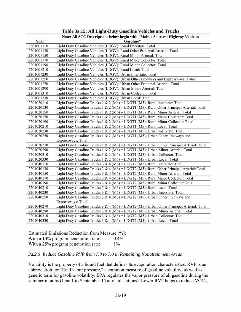
3a.2.4 Commuter Programs

Commuter programs recognize and support employers who provide incentives to employees to reduce light-duty vehicle emissions. Employers implement a wide range of incentives to affect change in employee commuting habits including transit subsidies, bike-friendly facilities, telecommuting policies, and preferred parking for vanpools and carpools. The commuter measure in this RIA reflects a mixed package of incentives.

This measure demonstrates the potential emissions reductions from providing commuter incentives to 10% and 25% of the commuter population in 2020.

We used the findings from a recent Best Workplaces for Commuters survey, which was an EPA sponsored employee trip reduction program, to estimate the potential emissions reductions from this measure.9 The BWC survey found that, on average, employees at workplaces with comprehensive commuter programs emit 15% fewer emissions than employees at workplaces that do not offer a comprehensive commuter program.

9 Herzog, E., Bricka, S., Audette, L., and Rockwell, J., 2005. Do Employee Commuter Benefits Reduce Vehicle Emissions and Fuel Consumption? Results of the Fall 2004 Best Workplaces for Commuters Survey, Transportation Research Record, Journal of the Transportation Research Board: Forthcoming.

3a-18

We believe that getting 10%–25% of the workforce involved in commuter programs is realistic. For modeling purposes, we divided the commuter programs measure into two program penetration rates: 10% and 25%. This was meant to provide flexibility to model a lower penetration rate for areas that need only low levels of emissions reductions to achieve attainment.

According to the 2001 National Household Transportation Survey (NHTS) published by DOT, commute VMT represents 27% of total VMT. Based on this information, we calculated that BWC would reduce light-duty gasoline emissions by 0.4% and 1% with a 10% and 25% program penetration rate, respectively.

Pollutants and Source Categories Affected by Measure (SCC): NOx, and VOC

3a-19

Table 3a.15: All Light-Duty Gasoline Vehicles and Trucks

SCC Note: All SCC Descriptions below begin with “Mobile Sources; Highway Vehicles—

Gasoline” 2201001110 Light Duty Gasoline Vehicles (LDGV); Rural Interstate: Total 2201001130 Light Duty Gasoline Vehicles (LDGV); Rural Other Principal Arterial: Total 2201001150 Light Duty Gasoline Vehicles (LDGV); Rural Minor Arterial: Total 2201001170 Light Duty Gasoline Vehicles (LDGV); Rural Major Collector: Total 2201001190 Light Duty Gasoline Vehicles (LDGV); Rural Minor Collector: Total 2201001210 Light Duty Gasoline Vehicles (LDGV); Rural Local: Total 2201001230 Light Duty Gasoline Vehicles (LDGV); Urban Interstate: Total 2201001250 Light Duty Gasoline Vehicles (LDGV); Urban Other Freeways and Expressways: Total 2201001270 Light Duty Gasoline Vehicles (LDGV); Urban Other Principal Arterial: Total 2201001290 Light Duty Gasoline Vehicles (LDGV); Urban Minor Arterial: Total 2201001310 Light Duty Gasoline Vehicles (LDGV); Urban Collector: Total 2201001330 Light Duty Gasoline Vehicles (LDGV); Urban Local: Total 2201020110 Light Duty Gasoline Trucks 1 & 2 (M6) = LDGT1 (M5); Rural Interstate: Total 2201020130 Light Duty Gasoline Trucks 1 & 2 (M6) = LDGT1 (M5); Rural Other Principal Arterial: Total 2201020150 Light Duty Gasoline Trucks 1 & 2 (M6) = LDGT1 (M5); Rural Minor Arterial: Total 2201020170 Light Duty Gasoline Trucks 1 & 2 (M6) = LDGT1 (M5); Rural Major Collector: Total 2201020190 Light Duty Gasoline Trucks 1 & 2 (M6) = LDGT1 (M5); Rural Minor Collector: Total 2201020210 Light Duty Gasoline Trucks 1 & 2 (M6) = LDGT1 (M5); Rural Local: Total 2201020230 Light Duty Gasoline Trucks 1 & 2 (M6) = LDGT1 (M5); Urban Interstate: Total 2201020250 Light Duty Gasoline Trucks 1 & 2 (M6) = LDGT1 (M5); Urban Other Freeways and

Expressways: Total 2201020270 Light Duty Gasoline Trucks 1 & 2 (M6) = LDGT1 (M5); Urban Other Principal Arterial: Total 2201020290 Light Duty Gasoline Trucks 1 & 2 (M6) = LDGT1 (M5); Urban Minor Arterial: Total 2201020310 Light Duty Gasoline Trucks 1 & 2 (M6) = LDGT1 (M5); Urban Collector: Total 2201020330 Light Duty Gasoline Trucks 1 & 2 (M6) = LDGT1 (M5); Urban Local: Total 2201040110 Light Duty Gasoline Trucks 3 & 4 (M6) = LDGT2 (M5); Rural Interstate: Total 2201040130 Light Duty Gasoline Trucks 3 & 4 (M6) = LDGT2 (M5); Rural Other Principal Arterial: Total 2201040150 Light Duty Gasoline Trucks 3 & 4 (M6) = LDGT2 (M5); Rural Minor Arterial: Total 2201040170 Light Duty Gasoline Trucks 3 & 4 (M6) = LDGT2 (M5); Rural Major Collector: Total 2201040190 Light Duty Gasoline Trucks 3 & 4 (M6) = LDGT2 (M5); Rural Minor Collector: Total 2201040210 Light Duty Gasoline Trucks 3 & 4 (M6) = LDGT2 (M5); Rural Local: Total 2201040230 Light Duty Gasoline Trucks 3 & 4 (M6) = LDGT2 (M5); Urban Interstate: Total 2201040250 Light Duty Gasoline Trucks 3 & 4 (M6) = LDGT2 (M5); Urban Other Freeways and

Expressways: Total 2201040270 Light Duty Gasoline Trucks 3 & 4 (M6) = LDGT2 (M5); Urban Other Principal Arterial: Total 2201040290 Light Duty Gasoline Trucks 3 & 4 (M6) = LDGT2 (M5); Urban Minor Arterial: Total 2201040310 Light Duty Gasoline Trucks 3 & 4 (M6) = LDGT2 (M5); Urban Collector: Total 2201040330 Light Duty Gasoline Trucks 3 & 4 (M6) = LDGT2 (M5); Urban Local: Total

Estimated Emissions Reduction from Measure (%): With a 10% program penetration rate: 0.4% With a 25% program penetration rate: 1%

3a.2.5 Reduce Gasoline RVP from 7.8 to 7.0 in Remaining Nonattainment Areas

Volatility is the property of a liquid fuel that defines its evaporation characteristics. RVP is an abbreviation for “Reid vapor pressure,” a common measure of gasoline volatility, as well as a generic term for gasoline volatility. EPA regulates the vapor pressure of all gasoline during the summer months (June 1 to September 15 at retail stations). Lower RVP helps to reduce VOCs,

3a-20

which are a precursor to ozone formation. This control measure represents the use of gasoline with a RVP limit of 7.0 psi from May through September in counties with an ozone season RVP value greater than 7.0 psi.

Under section 211(c)(4)(C) of the CAA, EPA may approve a non-identical state fuel control as a SIP provision, if the state demonstrates that the measure is necessary to achieve the national primary or secondary ambient air quality standard (NAAQS) that the plan implements. EPA can approve a state fuel requirement as necessary only if no other measures would bring about timely attainment, or if other measures exist but are unreasonable or impracticable.

Source Categories Affected by Measure:

• All light-duty gasoline vehicles and trucks: Affected SCC:

– 2201001000 Light Duty Gasoline Vehicles (LDGV), Total: All Road Types

– 2201020000 Light Duty Gasoline Trucks 1 (LDGT1), Total: All Road Types

– 2201040000 Light Duty Gasoline Trucks 2 (LDGT2), Total: All Road Types

– 2201070000 Heavy Duty Gasoline Vehicles (HDGV), Total: All Road Types

– 2201080000 Motorcycles (MC), Total: All Road Types

3a.3 EGU Controls Used in the Control Strategy

Table 3a.16 contains the ozone season emissions from all fossil EGU sources (greater than 25 megawatts) for the baseline and the control strategy.

Table 3a.16: NOx EGU Ozone Season Emissions (All Fossil Units >25MW) (1,000 Tons)a

OTC MWRPO East TX National CAIR Region

CAIR Cap

Baseline (CAIR/CAMR/CAVR)

73 154 43 828 463 485

Control Strategy 65 (−11%)

113 (−26%)

33 (−23%)

812 (−2%)

470 482

a Numbers in parentheses are the percentage change in emissions.

3a.3.1 CAIR

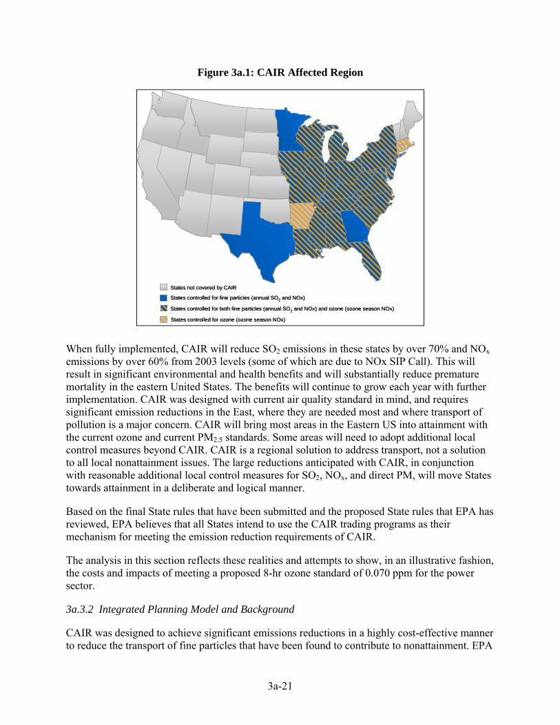
The data and projections presented in Section 3.2.2 cover the electric power sector, an industry that will achieve significant emission reductions under the Clean Air Interstate Rule (CAIR) over the next 10 to 15 years. Based on an assessment of the emissions contributing to interstate transport of air pollution and available control measures, EPA determined that achieving required reductions in the identified States by controlling emissions from power plants is highly cost effective. CAIR will permanently cap emissions of sulfur dioxide (SO2) and nitrogen oxides (NOx) in the eastern United States. CAIR achieves large reductions of SO2 and/or NOx emissions across 28 eastern states and the District of Columbia.

3a-21

Figure 3a.1: CAIR Affected Region

States controlled for fine particles (annual SO2 and NOx)States controlled for fine particles (annual SO2 and NOx)

States not covered by CAIRStates not covered by CAIR

States controlled for ozone (ozone season NOx)States controlled for ozone (ozone season NOx)

States controlled for both fine particles (annual SO2 and NOx) and ozone (ozone season NOx)States controlled for both fine particles (annual SO2 and NOx) and ozone (ozone season NOx)

When fully implemented, CAIR will reduce SO2 emissions in these states by over 70% and NOx emissions by over 60% from 2003 levels (some of which are due to NOx SIP Call). This will result in significant environmental and health benefits and will substantially reduce premature mortality in the eastern United States. The benefits will continue to grow each year with further implementation. CAIR was designed with current air quality standard in mind, and requires significant emission reductions in the East, where they are needed most and where transport of pollution is a major concern. CAIR will bring most areas in the Eastern US into attainment with the current ozone and current PM2.5 standards. Some areas will need to adopt additional local control measures beyond CAIR. CAIR is a regional solution to address transport, not a solution to all local nonattainment issues. The large reductions anticipated with CAIR, in conjunction with reasonable additional local control measures for SO2, NOx, and direct PM, will move States towards attainment in a deliberate and logical manner.

Based on the final State rules that have been submitted and the proposed State rules that EPA has reviewed, EPA believes that all States intend to use the CAIR trading programs as their mechanism for meeting the emission reduction requirements of CAIR.

The analysis in this section reflects these realities and attempts to show, in an illustrative fashion, the costs and impacts of meeting a proposed 8-hr ozone standard of 0.070 ppm for the power sector.

3a.3.2 Integrated Planning Model and Background

CAIR was designed to achieve significant emissions reductions in a highly cost-effective manner to reduce the transport of fine particles that have been found to contribute to nonattainment. EPA

3a-22

analysis has found that the most efficient method to achieve the emissions reduction targets is through a cap-and-trade system on the power sector that States have the option of adopting. The modeling done with IPM assumes a region-wide cap and trade system on the power sector for the States covered.

It is important to note that the proposal RIA analysis used the Integrated Planning Model (IPM) v2.1.9 to ensure consistency with the analysis presented in 2006 PM NAAQS RIA and report incremental results. EPA’s IPM v2.1.9 incorporated Federal and State rules and regulations adopted before March 2004 and various NSR settlements.

Final RIA analysis uses the latest version of IPM (v3.0) as part of the updated modeling platform. IPM v3.0 includes input and model assumption updates in modeling the power sector and incorporates Federal and State rules and regulations adopted before September 2006 and various NSR settlements. A detailed discussion of uncertainties associated with the EGU sector modeling can be found in 2006 PM NAAQS RIA (pg. 3-50)

The economic modeling using IPM presented in this and other chapters has been developed for specific analyses of the power sector. EPA’s modeling is based on its best judgment for various input assumptions that are uncertain, particularly assumptions for future fuel prices and electricity demand growth. To some degree, EPA addresses the uncertainty surrounding these two assumptions through sensitivity analyses. More detail on IPM can be found in the model documentation, which provides additional information on the assumptions discussed here as well as all other assumptions and inputs to the model (http://www.epa.gov/airmarkets/progsregs/epa-ipm.html).

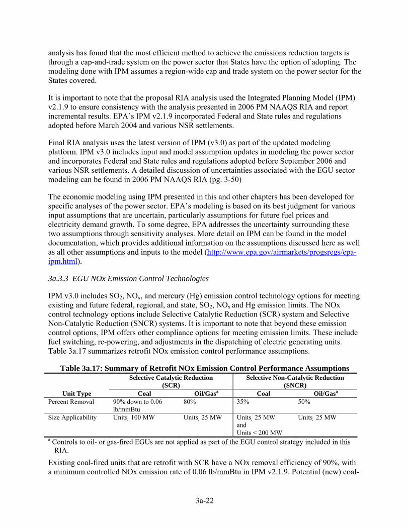
3a.3.3 EGU NOx Emission Control Technologies

IPM v3.0 includes SO2, NOx, and mercury (Hg) emission control technology options for meeting existing and future federal, regional, and state, SO2, NOx and Hg emission limits. The NOx control technology options include Selective Catalytic Reduction (SCR) system and Selective Non-Catalytic Reduction (SNCR) systems. It is important to note that beyond these emission control options, IPM offers other compliance options for meeting emission limits. These include fuel switching, re-powering, and adjustments in the dispatching of electric generating units. Table 3a.17 summarizes retrofit NOx emission control performance assumptions.

Table 3a.17: Summary of Retrofit NOx Emission Control Performance Assumptions

Selective Catalytic Reduction

(SCR) Selective Non-Catalytic Reduction

(SNCR) Unit Type Coal Oil/Gasa Coal Oil/Gasa

Percent Removal 90% down to 0.06 lb/mmBtu

80% 35% 50%

Size Applicability Units 100 MW Units 25 MW Units 25 MW and Units < 200 MW

Units 25 MW

a Controls to oil- or gas-fired EGUs are not applied as part of the EGU control strategy included in this RIA.

Existing coal-fired units that are retrofit with SCR have a NOx removal efficiency of 90%, with a minimum controlled NOx emission rate of 0.06 lb/mmBtu in IPM v2.1.9. Potential (new) coal-

3a-23

fired, combined cycle, and IGCC units are modeled to be constructed with SCR systems and designed to have emission rates ranging between 0.02 and 0.06 lb NOx/mmBtu.

Detailed cost and performance derivations for NOx controls are discussed in detail in the EPA’s documentation of IPM (http://www.epa.gov/airmarkets/progsregs/epa-ipm/past-modeling.html).

3a.4 Emissions Reductions by Sector

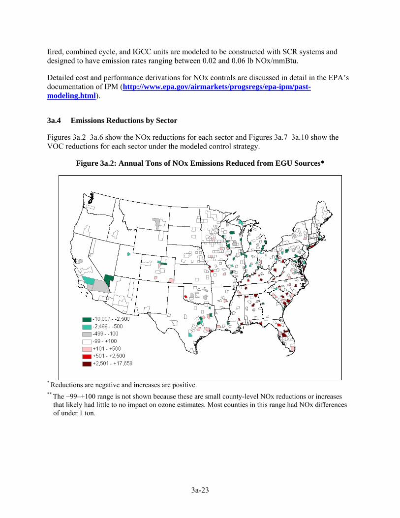
Figures 3a.2–3a.6 show the NOx reductions for each sector and Figures 3a.7–3a.10 show the VOC reductions for each sector under the modeled control strategy.

Figure 3a.2: Annual Tons of NOx Emissions Reduced from EGU Sources*

* Reductions are negative and increases are positive. ** The −99–+100 range is not shown because these are small county-level NOx reductions or increases

that likely had little to no impact on ozone estimates. Most counties in this range had NOx differences of under 1 ton.

3a-24

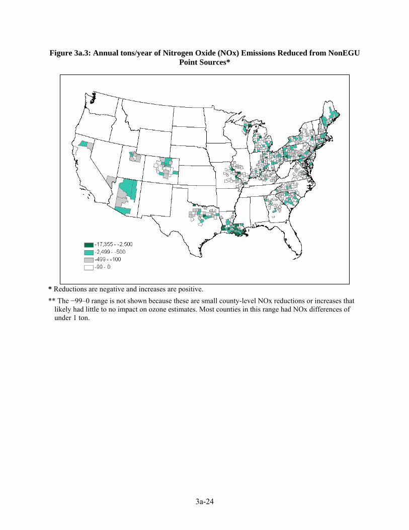
Figure 3a.3: Annual tons/year of Nitrogen Oxide (NOx) Emissions Reduced from NonEGU Point Sources*

* Reductions are negative and increases are positive. ** The −99–0 range is not shown because these are small county-level NOx reductions or increases that

likely had little to no impact on ozone estimates. Most counties in this range had NOx differences of under 1 ton.

3a-25

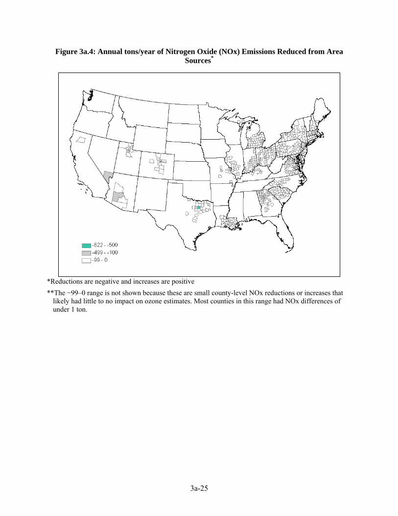
Figure 3a.4: Annual tons/year of Nitrogen Oxide (NOx) Emissions Reduced from Area Sources*

*Reductions are negative and increases are positive **The −99–0 range is not shown because these are small county-level NOx reductions or increases that


3a-26

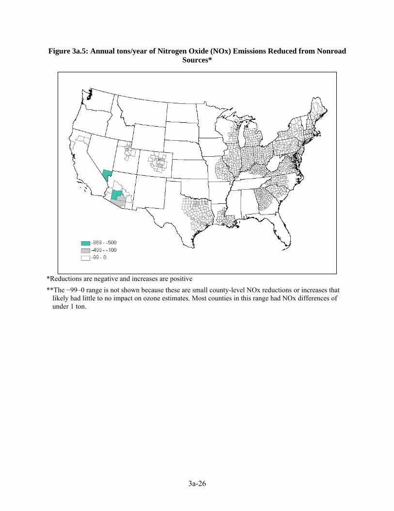
Figure 3a.5: Annual tons/year of Nitrogen Oxide (NOx) Emissions Reduced from Nonroad Sources*



3a-27

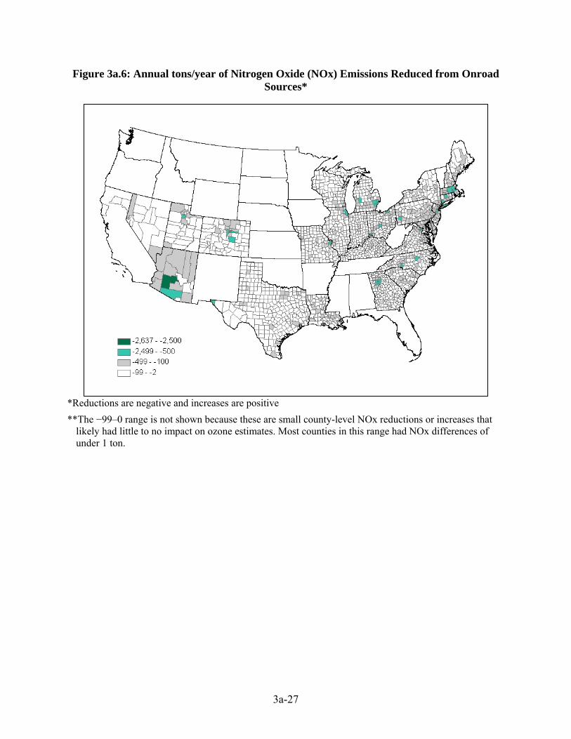
Figure 3a.6: Annual tons/year of Nitrogen Oxide (NOx) Emissions Reduced from Onroad Sources*



3a-28

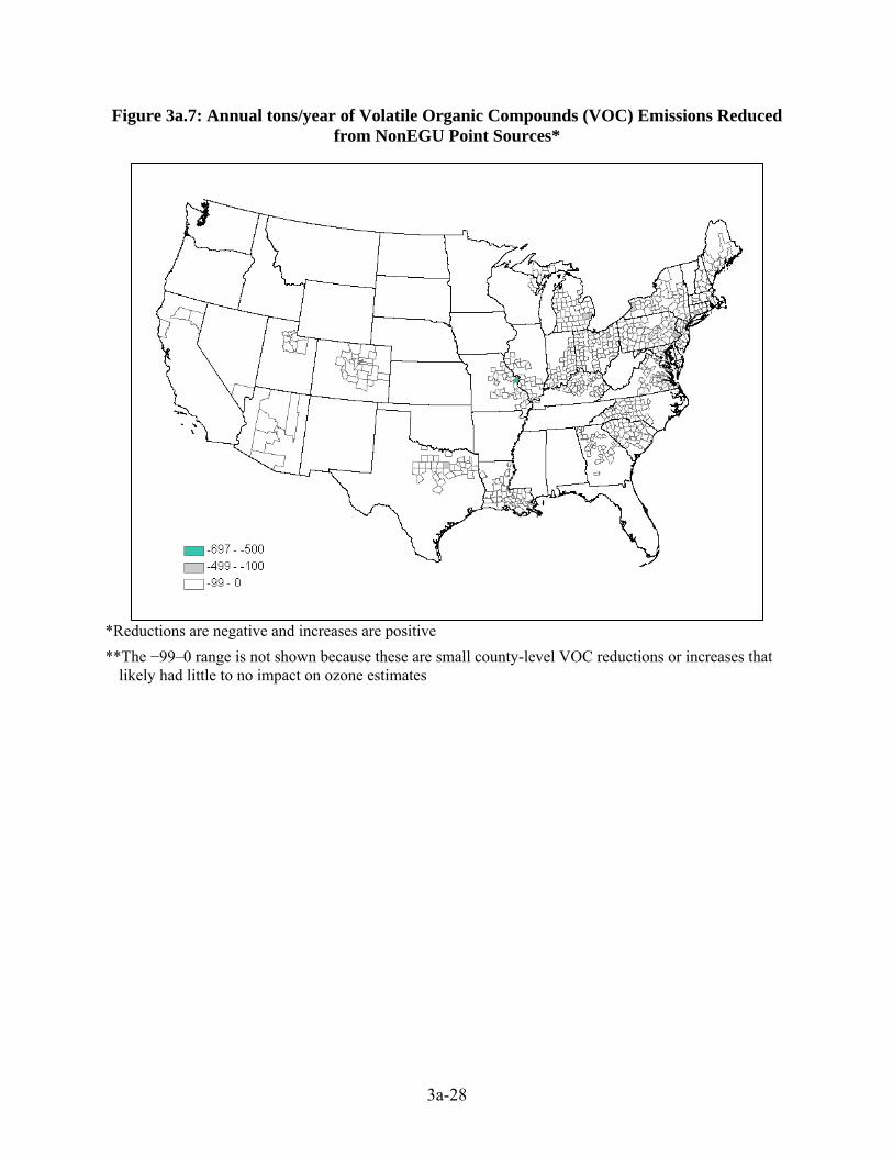
Figure 3a.7: Annual tons/year of Volatile Organic Compounds (VOC) Emissions Reduced from NonEGU Point Sources*

*Reductions are negative and increases are positive **The −99–0 range is not shown because these are small county-level VOC reductions or increases that

likely had little to no impact on ozone estimates

3a-29

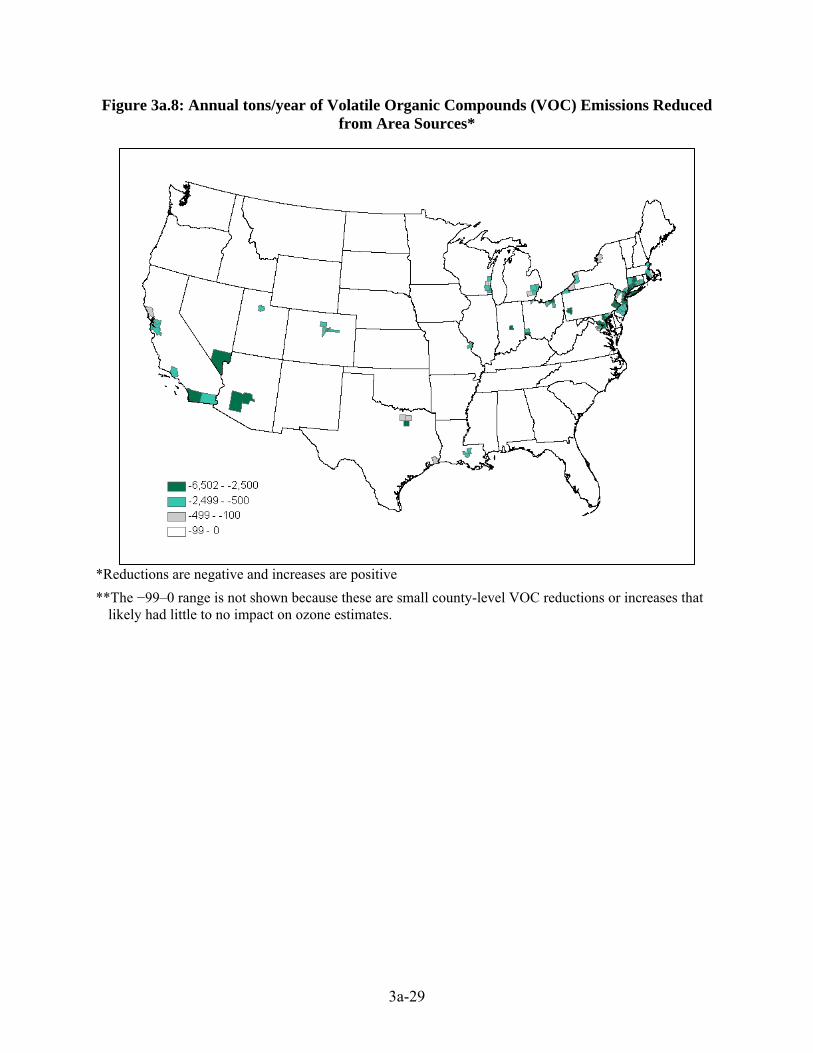
Figure 3a.8: Annual tons/year of Volatile Organic Compounds (VOC) Emissions Reduced from Area Sources*


likely had little to no impact on ozone estimates.

3a-30

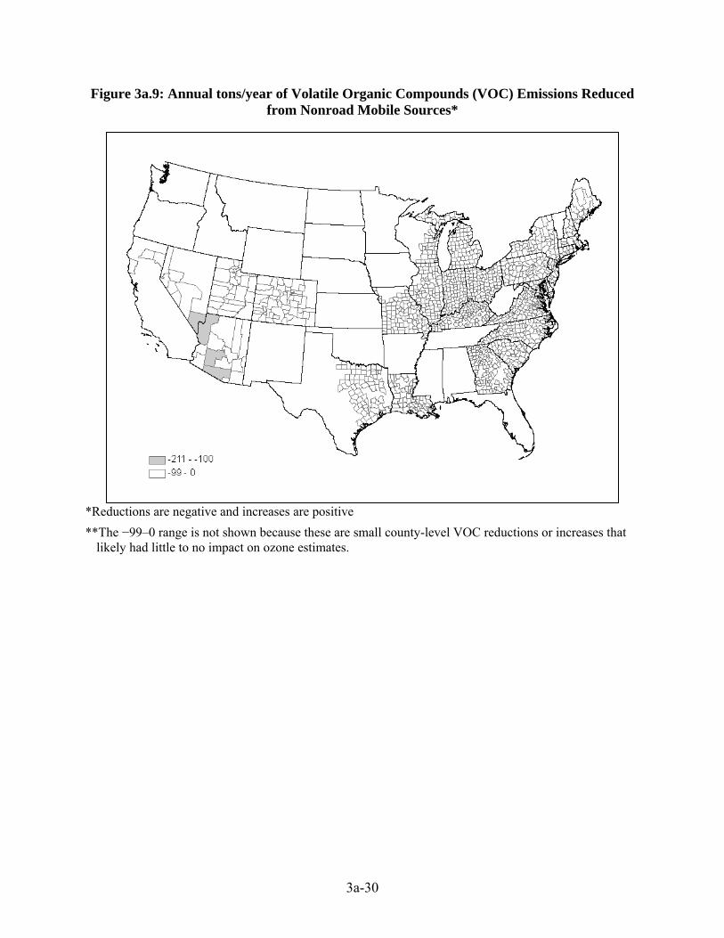
Figure 3a.9: Annual tons/year of Volatile Organic Compounds (VOC) Emissions Reduced from Nonroad Mobile Sources*



3a-31

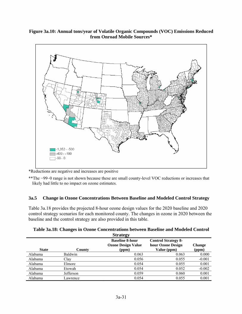
Figure 3a.10: Annual tons/year of Volatile Organic Compounds (VOC) Emissions Reduced from Onroad Mobile Sources*



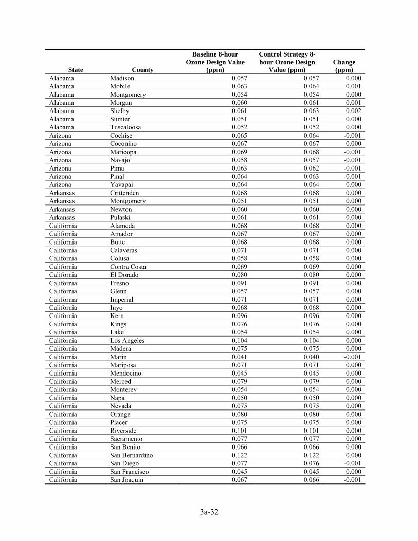
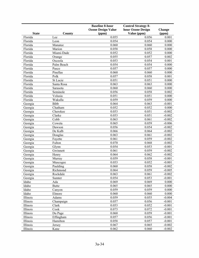
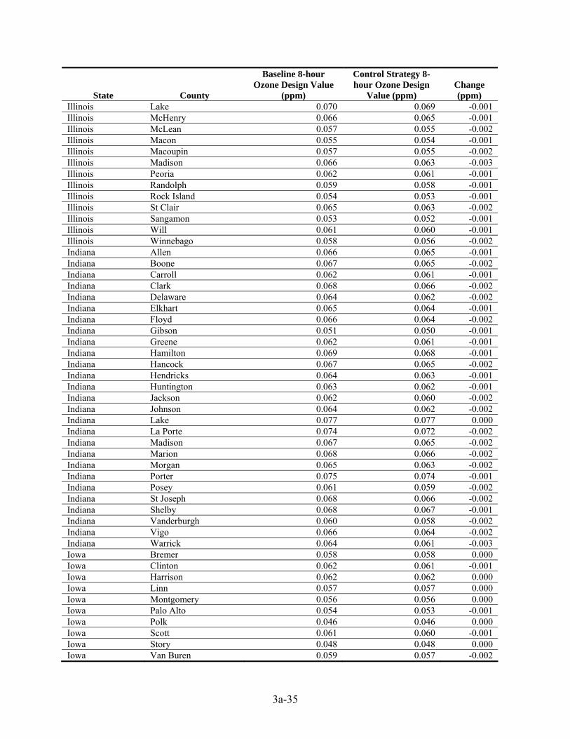
3a.5 Change in Ozone Concentrations Between Baseline and Modeled Control Strategy

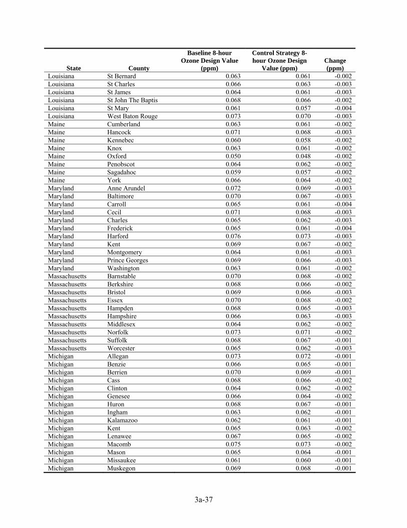
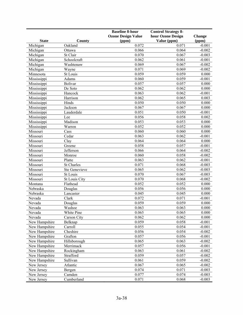
Table 3a.18 provides the projected 8-hour ozone design values for the 2020 baseline and 2020 control strategy scenarios for each monitored county. The changes in ozone in 2020 between the baseline and the control strategy are also provided in this table.

Table 3a.18: Changes in Ozone Concentrations between Baseline and Modeled Control Strategy

State County

Baseline 8-hour Ozone Design Value

(ppm)

Control Strategy 8-hour Ozone Design

Value (ppm) Change (ppm)

Alabama Baldwin 0.063 0.063 0.000 Alabama Clay 0.056 0.055 -0.001 Alabama Elmore 0.054 0.055 0.001 Alabama Etowah 0.054 0.052 -0.002 Alabama Jefferson 0.059 0.060 0.001 Alabama Lawrence 0.054 0.055 0.001

3a-32

State County


(ppm)



Alabama Madison 0.057 0.057 0.000 Alabama Mobile 0.063 0.064 0.001 Alabama Montgomery 0.054 0.054 0.000 Alabama Morgan 0.060 0.061 0.001 Alabama Shelby 0.061 0.063 0.002 Alabama Sumter 0.051 0.051 0.000 Alabama Tuscaloosa 0.052 0.052 0.000 Arizona Cochise 0.065 0.064 -0.001 Arizona Coconino 0.067 0.067 0.000 Arizona Maricopa 0.069 0.068 -0.001 Arizona Navajo 0.058 0.057 -0.001 Arizona Pima 0.063 0.062 -0.001 Arizona Pinal 0.064 0.063 -0.001 Arizona Yavapai 0.064 0.064 0.000 Arkansas Crittenden 0.068 0.068 0.000 Arkansas Montgomery 0.051 0.051 0.000 Arkansas Newton 0.060 0.060 0.000 Arkansas Pulaski 0.061 0.061 0.000 California Alameda 0.068 0.068 0.000 California Amador 0.067 0.067 0.000 California Butte 0.068 0.068 0.000 California Calaveras 0.071 0.071 0.000 California Colusa 0.058 0.058 0.000 California Contra Costa 0.069 0.069 0.000 California El Dorado 0.080 0.080 0.000 California Fresno 0.091 0.091 0.000 California Glenn 0.057 0.057 0.000 California Imperial 0.071 0.071 0.000 California Inyo 0.068 0.068 0.000 California Kern 0.096 0.096 0.000 California Kings 0.076 0.076 0.000 California Lake 0.054 0.054 0.000 California Los Angeles 0.104 0.104 0.000 California Madera 0.075 0.075 0.000 California Marin 0.041 0.040 -0.001 California Mariposa 0.071 0.071 0.000 California Mendocino 0.045 0.045 0.000 California Merced 0.079 0.079 0.000 California Monterey 0.054 0.054 0.000 California Napa 0.050 0.050 0.000 California Nevada 0.075 0.075 0.000 California Orange 0.080 0.080 0.000 California Placer 0.075 0.075 0.000 California Riverside 0.101 0.101 0.000 California Sacramento 0.077 0.077 0.000 California San Benito 0.066 0.066 0.000 California San Bernardino 0.122 0.122 0.000 California San Diego 0.077 0.076 -0.001 California San Francisco 0.045 0.045 0.000 California San Joaquin 0.067 0.066 -0.001

3a-33

State County


(ppm)



California San Luis Obispo 0.060 0.060 0.000 California San Mateo 0.051 0.050 -0.001 California Santa Barbara 0.068 0.068 0.000 California Santa Clara 0.066 0.066 0.000 California Santa Cruz 0.054 0.054 0.000 California Shasta 0.057 0.057 0.000 California Solano 0.057 0.057 0.000 California Sonoma 0.048 0.048 0.000 California Stanislaus 0.076 0.076 0.000 California Sutter 0.067 0.067 0.000 California Tehama 0.065 0.065 0.000 California Tulare 0.083 0.083 0.000 California Tuolumne 0.072 0.072 0.000 California Ventura 0.077 0.077 0.000 California Yolo 0.064 0.064 0.000 Colorado Adams 0.056 0.053 -0.003 Colorado Arapahoe 0.069 0.064 -0.005 Colorado Boulder 0.062 0.058 -0.004 Colorado Denver 0.064 0.060 -0.004 Colorado Douglas 0.072 0.067 -0.005 Colorado El Paso 0.062 0.059 -0.003 Colorado Jefferson 0.072 0.067 -0.005 Colorado La Plata 0.051 0.051 0.000 Colorado Larimer 0.066 0.061 -0.005 Colorado Montezuma 0.062 0.062 0.000 Colorado Weld 0.063 0.059 -0.004 Connecticut Fairfield 0.079 0.076 -0.003 Connecticut Hartford 0.065 0.062 -0.003 Connecticut Litchfield 0.064 0.061 -0.003 Connecticut Middlesex 0.073 0.070 -0.003 Connecticut New Haven 0.076 0.073 -0.003 Connecticut New London 0.067 0.065 -0.002 Connecticut Tolland 0.068 0.065 -0.003 Delaware Kent 0.069 0.067 -0.002 Delaware New Castle 0.070 0.067 -0.003 Delaware Sussex 0.070 0.067 -0.003 D.C. Washington 0.068 0.065 -0.003 Florida Alachua 0.056 0.056 0.000 Florida Baker 0.054 0.054 0.000 Florida Bay 0.061 0.063 0.002 Florida Brevard 0.050 0.051 0.001 Florida Broward 0.054 0.054 0.000 Florida Collier 0.056 0.056 0.000 Florida Columbia 0.052 0.052 0.000 Florida Duval 0.052 0.052 0.000 Florida Escambia 0.064 0.064 0.000 Florida Highlands 0.053 0.053 0.000 Florida Hillsborough 0.065 0.065 0.000 Florida Holmes 0.054 0.054 0.000 Florida Lake 0.054 0.056 0.002

3a-34

State County


(ppm)



Florida Lee 0.055 0.056 0.001 Florida Leon 0.054 0.054 0.000 Florida Manatee 0.060 0.060 0.000 Florida Marion 0.058 0.058 0.000 Florida Miami-Dade 0.052 0.052 0.000 Florida Orange 0.055 0.057 0.002 Florida Osceola 0.053 0.054 0.001 Florida Palm Beach 0.054 0.054 0.000 Florida Pasco 0.057 0.057 0.000 Florida Pinellas 0.060 0.060 0.000 Florida Polk 0.057 0.058 0.001 Florida St Lucie 0.051 0.051 0.000 Florida Santa Rosa 0.063 0.063 0.000 Florida Sarasota 0.060 0.060 0.000 Florida Seminole 0.056 0.058 0.002 Florida Volusia 0.051 0.051 0.000 Florida Wakulla 0.059 0.059 0.000 Georgia Bibb 0.064 0.063 -0.001 Georgia Chatham 0.052 0.052 0.000 Georgia Cherokee 0.053 0.051 -0.002 Georgia Clarke 0.053 0.051 -0.002 Georgia Cobb 0.063 0.061 -0.002 Georgia Coweta 0.065 0.059 -0.006 Georgia Dawson 0.056 0.054 -0.002 Georgia De Kalb 0.066 0.064 -0.002 Georgia Douglas 0.063 0.061 -0.002 Georgia Fayette 0.061 0.059 -0.002 Georgia Fulton 0.070 0.068 -0.002 Georgia Glynn 0.054 0.053 -0.001 Georgia Gwinnett 0.061 0.059 -0.002 Georgia Henry 0.064 0.062 -0.002 Georgia Murray 0.059 0.058 -0.001 Georgia Muscogee 0.053 0.052 -0.001 Georgia Paulding 0.060 0.058 -0.002 Georgia Richmond 0.064 0.059 -0.005 Georgia Rockdale 0.063 0.061 -0.002 Georgia Sumter 0.054 0.053 -0.001 Idaho Ada 0.069 0.069 0.000 Idaho Butte 0.065 0.065 0.000 Idaho Canyon 0.059 0.059 0.000 Idaho Elmore 0.060 0.060 0.000 Illinois Adams 0.059 0.055 -0.004 Illinois Champaign 0.057 0.056 -0.001 Illinois Clark 0.053 0.052 -0.001 Illinois Cook 0.073 0.072 -0.001 Illinois Du Page 0.060 0.059 -0.001 Illinois Effingham 0.057 0.056 -0.001 Illinois Hamilton 0.058 0.057 -0.001 Illinois Jersey 0.067 0.065 -0.002 Illinois Kane 0.062 0.060 -0.002

3a-35

State County


(ppm)



Illinois Lake 0.070 0.069 -0.001 Illinois McHenry 0.066 0.065 -0.001 Illinois McLean 0.057 0.055 -0.002 Illinois Macon 0.055 0.054 -0.001 Illinois Macoupin 0.057 0.055 -0.002 Illinois Madison 0.066 0.063 -0.003 Illinois Peoria 0.062 0.061 -0.001 Illinois Randolph 0.059 0.058 -0.001 Illinois Rock Island 0.054 0.053 -0.001 Illinois St Clair 0.065 0.063 -0.002 Illinois Sangamon 0.053 0.052 -0.001 Illinois Will 0.061 0.060 -0.001 Illinois Winnebago 0.058 0.056 -0.002 Indiana Allen 0.066 0.065 -0.001 Indiana Boone 0.067 0.065 -0.002 Indiana Carroll 0.062 0.061 -0.001 Indiana Clark 0.068 0.066 -0.002 Indiana Delaware 0.064 0.062 -0.002 Indiana Elkhart 0.065 0.064 -0.001 Indiana Floyd 0.066 0.064 -0.002 Indiana Gibson 0.051 0.050 -0.001 Indiana Greene 0.062 0.061 -0.001 Indiana Hamilton 0.069 0.068 -0.001 Indiana Hancock 0.067 0.065 -0.002 Indiana Hendricks 0.064 0.063 -0.001 Indiana Huntington 0.063 0.062 -0.001 Indiana Jackson 0.062 0.060 -0.002 Indiana Johnson 0.064 0.062 -0.002 Indiana Lake 0.077 0.077 0.000 Indiana La Porte 0.074 0.072 -0.002 Indiana Madison 0.067 0.065 -0.002 Indiana Marion 0.068 0.066 -0.002 Indiana Morgan 0.065 0.063 -0.002 Indiana Porter 0.075 0.074 -0.001 Indiana Posey 0.061 0.059 -0.002 Indiana St Joseph 0.068 0.066 -0.002 Indiana Shelby 0.068 0.067 -0.001 Indiana Vanderburgh 0.060 0.058 -0.002 Indiana Vigo 0.066 0.064 -0.002 Indiana Warrick 0.064 0.061 -0.003 Iowa Bremer 0.058 0.058 0.000 Iowa Clinton 0.062 0.061 -0.001 Iowa Harrison 0.062 0.062 0.000 Iowa Linn 0.057 0.057 0.000 Iowa Montgomery 0.056 0.056 0.000 Iowa Palo Alto 0.054 0.053 -0.001 Iowa Polk 0.046 0.046 0.000 Iowa Scott 0.061 0.060 -0.001 Iowa Story 0.048 0.048 0.000 Iowa Van Buren 0.059 0.057 -0.002

3a-36

State County


(ppm)



Iowa Warren 0.049 0.048 -0.001 Kansas Linn 0.060 0.059 -0.001 Kansas Sedgwick 0.063 0.063 0.000 Kansas Sumner 0.062 0.062 0.000 Kansas Trego 0.055 0.055 0.000 Kansas Wyandotte 0.062 0.062 0.000 Kentucky Bell 0.056 0.055 -0.001 Kentucky Boone 0.063 0.060 -0.003 Kentucky Boyd 0.070 0.069 -0.001 Kentucky Bullitt 0.061 0.059 -0.002 Kentucky Campbell 0.070 0.067 -0.003 Kentucky Carter 0.057 0.056 -0.001 Kentucky Christian 0.057 0.057 0.000 Kentucky Daviess 0.058 0.058 0.000 Kentucky Edmonson 0.059 0.057 -0.002 Kentucky Fayette 0.057 0.055 -0.002 Kentucky Graves 0.059 0.058 -0.001 Kentucky Greenup 0.064 0.063 -0.001 Kentucky Hancock 0.063 0.064 0.001 Kentucky Hardin 0.057 0.056 -0.001 Kentucky Henderson 0.060 0.057 -0.003 Kentucky Jefferson 0.064 0.063 -0.001 Kentucky Jessamine 0.057 0.056 -0.001 Kentucky Kenton 0.065 0.062 -0.003 Kentucky Livingston 0.061 0.060 -0.001 Kentucky McCracken 0.063 0.062 -0.001 Kentucky McLean 0.059 0.058 -0.001 Kentucky Oldham 0.063 0.061 -0.002 Kentucky Perry 0.055 0.054 -0.001 Kentucky Pike 0.054 0.053 -0.001 Kentucky Pulaski 0.058 0.060 0.002 Kentucky Scott 0.050 0.049 -0.001 Kentucky Simpson 0.056 0.056 0.000 Kentucky Trigg 0.052 0.052 0.000 Kentucky Warren 0.060 0.058 -0.002 Louisiana Ascension 0.068 0.065 -0.003 Louisiana Beauregard 0.061 0.058 -0.003 Louisiana Bossier 0.060 0.060 0.000 Louisiana Caddo 0.058 0.057 -0.001 Louisiana Calcasieu 0.066 0.063 -0.003 Louisiana East Baton Rouge 0.076 0.073 -0.003 Louisiana Grant 0.060 0.058 -0.002 Louisiana Iberville 0.072 0.068 -0.004 Louisiana Jefferson 0.069 0.066 -0.003 Louisiana Lafayette 0.065 0.061 -0.004 Louisiana Lafourche 0.065 0.062 -0.003 Louisiana Livingston 0.068 0.064 -0.004 Louisiana Orleans 0.057 0.056 -0.001 Louisiana Ouachita 0.061 0.060 -0.001 Louisiana Pointe Coupee 0.063 0.057 -0.006

3a-37

State County


(ppm)



Louisiana St Bernard 0.063 0.061 -0.002 Louisiana St Charles 0.066 0.063 -0.003 Louisiana St James 0.064 0.061 -0.003 Louisiana St John The Baptis 0.068 0.066 -0.002 Louisiana St Mary 0.061 0.057 -0.004 Louisiana West Baton Rouge 0.073 0.070 -0.003 Maine Cumberland 0.063 0.061 -0.002 Maine Hancock 0.071 0.068 -0.003 Maine Kennebec 0.060 0.058 -0.002 Maine Knox 0.063 0.061 -0.002 Maine Oxford 0.050 0.048 -0.002 Maine Penobscot 0.064 0.062 -0.002 Maine Sagadahoc 0.059 0.057 -0.002 Maine York 0.066 0.064 -0.002 Maryland Anne Arundel 0.072 0.069 -0.003 Maryland Baltimore 0.070 0.067 -0.003 Maryland Carroll 0.065 0.061 -0.004 Maryland Cecil 0.071 0.068 -0.003 Maryland Charles 0.065 0.062 -0.003 Maryland Frederick 0.065 0.061 -0.004 Maryland Harford 0.076 0.073 -0.003 Maryland Kent 0.069 0.067 -0.002 Maryland Montgomery 0.064 0.061 -0.003 Maryland Prince Georges 0.069 0.066 -0.003 Maryland Washington 0.063 0.061 -0.002 Massachusetts Barnstable 0.070 0.068 -0.002 Massachusetts Berkshire 0.068 0.066 -0.002 Massachusetts Bristol 0.069 0.066 -0.003 Massachusetts Essex 0.070 0.068 -0.002 Massachusetts Hampden 0.068 0.065 -0.003 Massachusetts Hampshire 0.066 0.063 -0.003 Massachusetts Middlesex 0.064 0.062 -0.002 Massachusetts Norfolk 0.073 0.071 -0.002 Massachusetts Suffolk 0.068 0.067 -0.001 Massachusetts Worcester 0.065 0.062 -0.003 Michigan Allegan 0.073 0.072 -0.001 Michigan Benzie 0.066 0.065 -0.001 Michigan Berrien 0.070 0.069 -0.001 Michigan Cass 0.068 0.066 -0.002 Michigan Clinton 0.064 0.062 -0.002 Michigan Genesee 0.066 0.064 -0.002 Michigan Huron 0.068 0.067 -0.001 Michigan Ingham 0.063 0.062 -0.001 Michigan Kalamazoo 0.062 0.061 -0.001 Michigan Kent 0.065 0.063 -0.002 Michigan Lenawee 0.067 0.065 -0.002 Michigan Macomb 0.075 0.073 -0.002 Michigan Mason 0.065 0.064 -0.001 Michigan Missaukee 0.061 0.060 -0.001 Michigan Muskegon 0.069 0.068 -0.001

3a-38

State County


(ppm)



Michigan Oakland 0.072 0.071 -0.001 Michigan Ottawa 0.066 0.064 -0.002 Michigan St Clair 0.070 0.067 -0.003 Michigan Schoolcraft 0.062 0.061 -0.001 Michigan Washtenaw 0.069 0.067 -0.002 Michigan Wayne 0.071 0.069 -0.002 Minnesota St Louis 0.059 0.059 0.000 Mississippi Adams 0.060 0.059 -0.001 Mississippi Bolivar 0.057 0.057 0.000 Mississippi De Soto 0.062 0.062 0.000 Mississippi Hancock 0.063 0.062 -0.001 Mississippi Harrison 0.062 0.065 0.003 Mississippi Hinds 0.050 0.050 0.000 Mississippi Jackson 0.067 0.067 0.000 Mississippi Lauderdale 0.051 0.050 -0.001 Mississippi Lee 0.056 0.058 0.002 Mississippi Madison 0.053 0.053 0.000 Mississippi Warren 0.052 0.052 0.000 Missouri Cass 0.060 0.060 0.000 Missouri Cedar 0.063 0.062 -0.001 Missouri Clay 0.064 0.064 0.000 Missouri Greene 0.058 0.057 -0.001 Missouri Jefferson 0.066 0.064 -0.002 Missouri Monroe 0.060 0.058 -0.002 Missouri Platte 0.063 0.062 -0.001 Missouri St Charles 0.071 0.068 -0.003 Missouri Ste Genevieve 0.065 0.062 -0.003 Missouri St Louis 0.070 0.067 -0.003 Missouri St Louis City 0.070 0.068 -0.002 Montana Flathead 0.052 0.052 0.000 Nebraska Douglas 0.056 0.056 0.000 Nebraska Lancaster 0.045 0.045 0.000 Nevada Clark 0.072 0.071 -0.001 Nevada Douglas 0.059 0.059 0.000 Nevada Washoe 0.063 0.063 0.000 Nevada White Pine 0.065 0.065 0.000 Nevada Carson City 0.062 0.062 0.000 New Hampshire Belknap 0.059 0.058 -0.001 New Hampshire Carroll 0.055 0.054 -0.001 New Hampshire Cheshire 0.056 0.054 -0.002 New Hampshire Grafton 0.057 0.056 -0.001 New Hampshire Hillsborough 0.065 0.063 -0.002 New Hampshire Merrimack 0.057 0.056 -0.001 New Hampshire Rockingham 0.063 0.061 -0.002 New Hampshire Strafford 0.059 0.057 -0.002 New Hampshire Sullivan 0.061 0.059 -0.002 New Jersey Atlantic 0.067 0.065 -0.002 New Jersey Bergen 0.074 0.071 -0.003 New Jersey Camden 0.077 0.074 -0.003 New Jersey Cumberland 0.071 0.068 -0.003

3a-39

State County


(ppm)



New Jersey Essex 0.052 0.051 -0.001 New Jersey Gloucester 0.075 0.073 -0.002 New Jersey Hudson 0.066 0.064 -0.002 New Jersey Hunterdon 0.071 0.068 -0.003 New Jersey Mercer 0.075 0.073 -0.002 New Jersey Middlesex 0.073 0.070 -0.003 New Jersey Monmouth 0.073 0.070 -0.003 New Jersey Morris 0.071 0.068 -0.003 New Jersey Ocean 0.079 0.076 -0.003 New Jersey Passaic 0.067 0.064 -0.003 New Mexico Bernalillo 0.065 0.064 -0.001 New Mexico Dona Ana 0.069 0.068 -0.001 New Mexico Eddy 0.063 0.063 0.000 New Mexico Sandoval 0.063 0.063 0.000 New Mexico San Juan 0.069 0.069 0.000 New Mexico Valencia 0.056 0.056 0.000 New York Albany 0.064 0.061 -0.003 New York Bronx 0.069 0.067 -0.002 New York Chautauqua 0.072 0.069 -0.003 New York Chemung 0.061 0.059 -0.002 New York Dutchess 0.068 0.065 -0.003 New York Erie 0.075 0.072 -0.003 New York Essex 0.069 0.067 -0.002 New York Hamilton 0.063 0.062 -0.001 New York Herkimer 0.059 0.057 -0.002 New York Jefferson 0.073 0.071 -0.002 New York Madison 0.062 0.060 -0.002 New York Monroe 0.067 0.064 -0.003 New York Niagara 0.075 0.073 -0.002 New York Oneida 0.063 0.061 -0.002 New York Onondaga 0.067 0.065 -0.002 New York Orange 0.063 0.061 -0.002 New York Oswego 0.053 0.052 -0.001 New York Putnam 0.070 0.068 -0.002 New York Queens 0.069 0.067 -0.002 New York Rensselaer 0.066 0.063 -0.003 New York Richmond 0.073 0.071 -0.002 New York Saratoga 0.067 0.063 -0.004 New York Schenectady 0.061 0.059 -0.002 New York Suffolk 0.080 0.077 -0.003 New York Ulster 0.063 0.061 -0.002 New York Wayne 0.065 0.063 -0.002 New York Westchester 0.074 0.071 -0.003 North Carolina Alexander 0.062 0.061 -0.001 North Carolina Avery 0.059 0.057 -0.002 North Carolina Buncombe 0.060 0.059 -0.001 North Carolina Caldwell 0.060 0.060 0.000 North Carolina Caswell 0.060 0.059 -0.001 North Carolina Chatham 0.058 0.057 -0.001 North Carolina Cumberland 0.061 0.060 -0.001

3a-40

State County


(ppm)



North Carolina Davie 0.064 0.062 -0.002 North Carolina Duplin 0.059 0.058 -0.001 North Carolina Durham 0.061 0.060 -0.001 North Carolina Edgecombe 0.063 0.062 -0.001 North Carolina Forsyth 0.063 0.062 -0.001 North Carolina Franklin 0.063 0.062 -0.001 North Carolina Granville 0.064 0.063 -0.001 North Carolina Guilford 0.060 0.058 -0.002 North Carolina Haywood 0.064 0.064 0.000 North Carolina Jackson 0.063 0.062 -0.001 North Carolina Johnston 0.060 0.059 -0.001 North Carolina Lenoir 0.060 0.059 -0.001 North Carolina Lincoln 0.064 0.065 0.001 North Carolina Martin 0.060 0.059 -0.001 North Carolina Mecklenburg 0.071 0.070 -0.001 North Carolina New Hanover 0.056 0.057 0.001 North Carolina Northampton 0.062 0.060 -0.002 North Carolina Person 0.063 0.061 -0.002 North Carolina Pitt 0.059 0.058 -0.001 North Carolina Randolph 0.057 0.056 -0.001 North Carolina Rockingham 0.062 0.061 -0.001 North Carolina Rowan 0.068 0.067 -0.001 North Carolina Swain 0.053 0.052 -0.001 North Carolina Union 0.062 0.061 -0.001 North Carolina Wake 0.064 0.063 -0.001 North Carolina Yancey 0.063 0.061 -0.002 North Dakota Billings 0.054 0.054 0.000 North Dakota Cass 0.055 0.055 0.000 North Dakota Dunn 0.054 0.054 0.000 North Dakota McKenzie 0.058 0.058 0.000 North Dakota Mercer 0.055 0.055 0.000 North Dakota Oliver 0.051 0.050 -0.001 Ohio Allen 0.068 0.065 -0.003 Ohio Ashtabula 0.075 0.073 -0.002 Ohio Butler 0.068 0.064 -0.004 Ohio Clark 0.066 0.062 -0.004 Ohio Clermont 0.068 0.066 -0.002 Ohio Clinton 0.069 0.066 -0.003 Ohio Cuyahoga 0.067 0.065 -0.002 Ohio Delaware 0.066 0.064 -0.002 Ohio Franklin 0.068 0.066 -0.002 Ohio Geauga 0.076 0.074 -0.002 Ohio Greene 0.066 0.062 -0.004 Ohio Hamilton 0.069 0.066 -0.003 Ohio Jefferson 0.063 0.061 -0.002 Ohio Knox 0.064 0.062 -0.002 Ohio Lake 0.072 0.070 -0.002 Ohio Lawrence 0.065 0.063 -0.002 Ohio Licking 0.065 0.062 -0.003 Ohio Lorain 0.067 0.065 -0.002

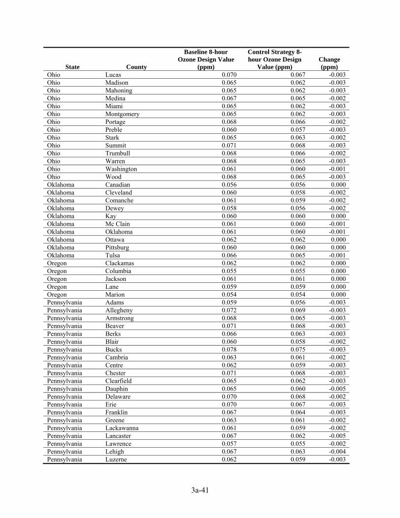
3a-41

State County


(ppm)



Ohio Lucas 0.070 0.067 -0.003 Ohio Madison 0.065 0.062 -0.003 Ohio Mahoning 0.065 0.062 -0.003 Ohio Medina 0.067 0.065 -0.002 Ohio Miami 0.065 0.062 -0.003 Ohio Montgomery 0.065 0.062 -0.003 Ohio Portage 0.068 0.066 -0.002 Ohio Preble 0.060 0.057 -0.003 Ohio Stark 0.065 0.063 -0.002 Ohio Summit 0.071 0.068 -0.003 Ohio Trumbull 0.068 0.066 -0.002 Ohio Warren 0.068 0.065 -0.003 Ohio Washington 0.061 0.060 -0.001 Ohio Wood 0.068 0.065 -0.003 Oklahoma Canadian 0.056 0.056 0.000 Oklahoma Cleveland 0.060 0.058 -0.002 Oklahoma Comanche 0.061 0.059 -0.002 Oklahoma Dewey 0.058 0.056 -0.002 Oklahoma Kay 0.060 0.060 0.000 Oklahoma Mc Clain 0.061 0.060 -0.001 Oklahoma Oklahoma 0.061 0.060 -0.001 Oklahoma Ottawa 0.062 0.062 0.000 Oklahoma Pittsburg 0.060 0.060 0.000 Oklahoma Tulsa 0.066 0.065 -0.001 Oregon Clackamas 0.062 0.062 0.000 Oregon Columbia 0.055 0.055 0.000 Oregon Jackson 0.061 0.061 0.000 Oregon Lane 0.059 0.059 0.000 Oregon Marion 0.054 0.054 0.000 Pennsylvania Adams 0.059 0.056 -0.003 Pennsylvania Allegheny 0.072 0.069 -0.003 Pennsylvania Armstrong 0.068 0.065 -0.003 Pennsylvania Beaver 0.071 0.068 -0.003 Pennsylvania Berks 0.066 0.063 -0.003 Pennsylvania Blair 0.060 0.058 -0.002 Pennsylvania Bucks 0.078 0.075 -0.003 Pennsylvania Cambria 0.063 0.061 -0.002 Pennsylvania Centre 0.062 0.059 -0.003 Pennsylvania Chester 0.071 0.068 -0.003 Pennsylvania Clearfield 0.065 0.062 -0.003 Pennsylvania Dauphin 0.065 0.060 -0.005 Pennsylvania Delaware 0.070 0.068 -0.002 Pennsylvania Erie 0.070 0.067 -0.003 Pennsylvania Franklin 0.067 0.064 -0.003 Pennsylvania Greene 0.063 0.061 -0.002 Pennsylvania Lackawanna 0.061 0.059 -0.002 Pennsylvania Lancaster 0.067 0.062 -0.005 Pennsylvania Lawrence 0.057 0.055 -0.002 Pennsylvania Lehigh 0.067 0.063 -0.004 Pennsylvania Luzerne 0.062 0.059 -0.003

3a-42

State County


(ppm)



Pennsylvania Lycoming 0.061 0.059 -0.002 Pennsylvania Mercer 0.068 0.065 -0.003 Pennsylvania Montgomery 0.071 0.068 -0.003 Pennsylvania Northampton 0.066 0.062 -0.004 Pennsylvania Perry 0.061 0.058 -0.003 Pennsylvania Philadelphia 0.077 0.074 -0.003 Pennsylvania Tioga 0.064 0.062 -0.002 Pennsylvania Washington 0.066 0.063 -0.003 Pennsylvania Westmoreland 0.068 0.065 -0.003 Pennsylvania York 0.067 0.062 -0.005 Rhode Island Kent 0.069 0.067 -0.002 Rhode Island Providence 0.069 0.066 -0.003 Rhode Island Washington 0.070 0.068 -0.002 South Carolina Abbeville 0.060 0.058 -0.002 South Carolina Aiken 0.061 0.058 -0.003 South Carolina Anderson 0.063 0.062 -0.001 South Carolina Barnwell 0.058 0.056 -0.002 South Carolina Berkeley 0.052 0.052 0.000 South Carolina Charleston 0.054 0.054 0.000 South Carolina Cherokee 0.061 0.059 -0.002 South Carolina Chester 0.059 0.058 -0.001 South Carolina Chesterfield 0.058 0.058 0.000 South Carolina Colleton 0.058 0.057 -0.001 South Carolina Darlington 0.061 0.060 -0.001 South Carolina Edgefield 0.059 0.056 -0.003 South Carolina Oconee 0.060 0.059 -0.001 South Carolina Pickens 0.059 0.058 -0.001 South Carolina Richland 0.066 0.064 -0.002 South Carolina Spartanburg 0.062 0.061 -0.001 South Carolina Union 0.058 0.057 -0.001 South Carolina Williamsburg 0.052 0.051 -0.001 South Carolina York 0.059 0.058 -0.001 South Dakota Pennington 0.062 0.061 -0.001 Tennessee Anderson 0.058 0.058 0.000 Tennessee Blount 0.064 0.064 0.000 Tennessee Davidson 0.056 0.056 0.000 Tennessee Hamilton 0.061 0.062 0.001 Tennessee Haywood 0.060 0.062 0.002 Tennessee Jefferson 0.061 0.061 0.000 Tennessee Knox 0.061 0.061 0.000 Tennessee Lawrence 0.056 0.058 0.002 Tennessee Meigs 0.061 0.060 -0.001 Tennessee Putnam 0.061 0.061 0.000 Tennessee Rutherford 0.058 0.057 -0.001 Tennessee Sevier 0.066 0.065 -0.001 Tennessee Shelby 0.065 0.065 0.000 Tennessee Sullivan 0.066 0.066 0.000 Tennessee Sumner 0.061 0.061 0.000 Tennessee Williamson 0.060 0.060 0.000 Tennessee Wilson 0.060 0.060 0.000

3a-43

State County


(ppm)



Texas Bexar 0.068 0.067 -0.001 Texas Brazoria 0.073 0.072 -0.001 Texas Brewster 0.054 0.053 -0.001 Texas Cameron 0.052 0.051 -0.001 Texas Collin 0.069 0.067 -0.002 Texas Dallas 0.068 0.066 -0.002 Texas Denton 0.074 0.072 -0.002 Texas Ellis 0.063 0.059 -0.004 Texas El Paso 0.069 0.068 -0.001 Texas Galveston 0.074 0.072 -0.002 Texas Gregg 0.067 0.064 -0.003 Texas Harris 0.089 0.087 -0.002 Texas Harrison 0.061 0.058 -0.003 Texas Hidalgo 0.062 0.061 -0.001 Texas Hood 0.058 0.056 -0.002 Texas Jefferson 0.074 0.071 -0.003 Texas Johnson 0.065 0.062 -0.003 Texas Kaufman 0.054 0.052 -0.002 Texas Montgomery 0.073 0.072 -0.001 Texas Nueces 0.065 0.063 -0.002 Texas Orange 0.066 0.063 -0.003 Texas Parker 0.063 0.061 -0.002 Texas Rockwall 0.061 0.060 -0.001 Texas Smith 0.064 0.061 -0.003 Texas Tarrant 0.075 0.073 -0.002 Texas Travis 0.063 0.062 -0.001 Texas Victoria 0.060 0.059 -0.001 Texas Webb 0.053 0.053 0.000 Utah Box Elder 0.064 0.062 -0.002 Utah Cache 0.056 0.054 -0.002 Utah Davis 0.070 0.067 -0.003 Utah Salt Lake 0.069 0.067 -0.002 Utah San Juan 0.064 0.063 -0.001 Utah Utah 0.067 0.065 -0.002 Utah Weber 0.065 0.062 -0.003 Vermont Bennington 0.061 0.058 -0.003 Vermont Chittenden 0.063 0.062 -0.001 Virginia Arlington 0.072 0.068 -0.004 Virginia Caroline 0.059 0.057 -0.002 Virginia Charles City 0.069 0.066 -0.003 Virginia Chesterfield 0.066 0.064 -0.002 Virginia Fairfax 0.071 0.067 -0.004 Virginia Fauquier 0.058 0.056 -0.002 Virginia Frederick 0.061 0.060 -0.001 Virginia Hanover 0.069 0.067 -0.002 Virginia Henrico 0.067 0.065 -0.002 Virginia Loudoun 0.066 0.063 -0.003 Virginia Madison 0.062 0.061 -0.001 Virginia Page 0.058 0.056 -0.002 Virginia Prince William 0.063 0.060 -0.003

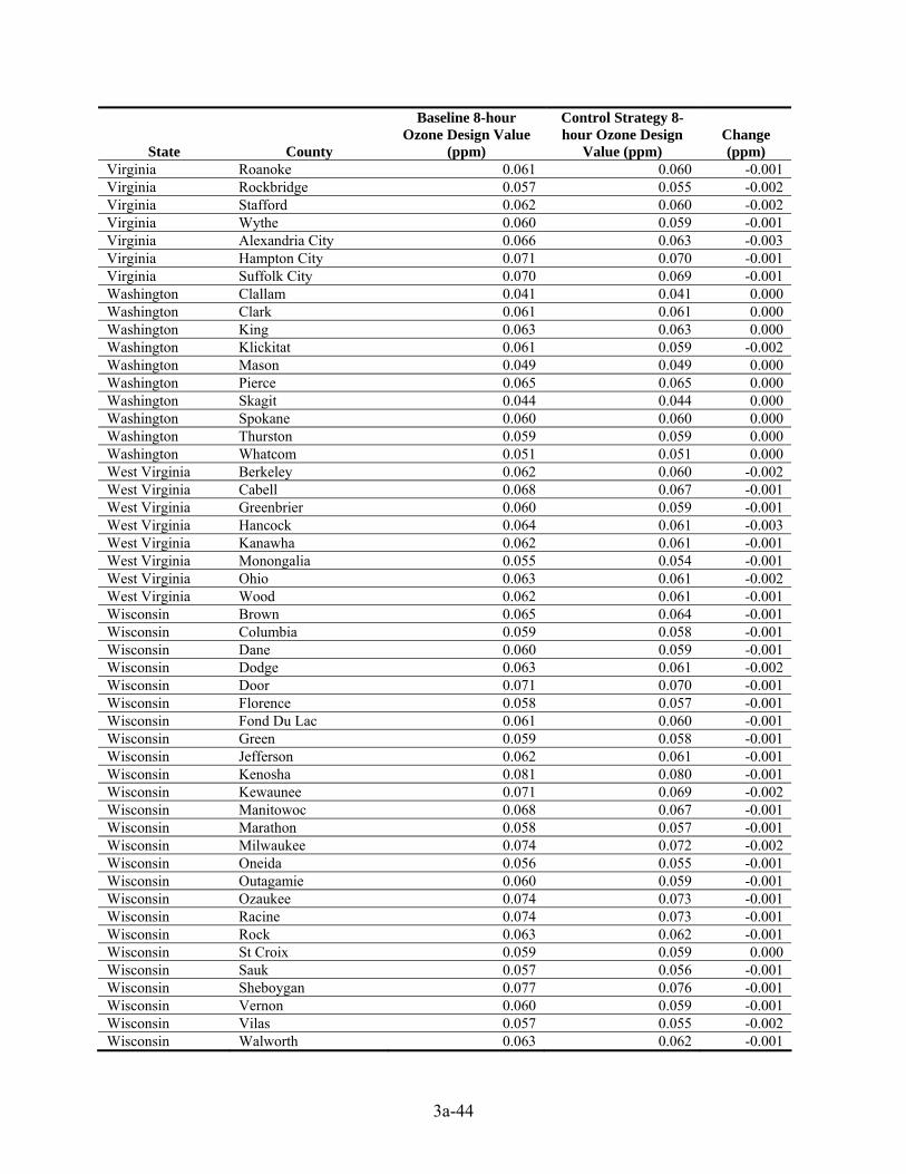
3a-44

State County


(ppm)



Virginia Roanoke 0.061 0.060 -0.001 Virginia Rockbridge 0.057 0.055 -0.002 Virginia Stafford 0.062 0.060 -0.002 Virginia Wythe 0.060 0.059 -0.001 Virginia Alexandria City 0.066 0.063 -0.003 Virginia Hampton City 0.071 0.070 -0.001 Virginia Suffolk City 0.070 0.069 -0.001 Washington Clallam 0.041 0.041 0.000 Washington Clark 0.061 0.061 0.000 Washington King 0.063 0.063 0.000 Washington Klickitat 0.061 0.059 -0.002 Washington Mason 0.049 0.049 0.000 Washington Pierce 0.065 0.065 0.000 Washington Skagit 0.044 0.044 0.000 Washington Spokane 0.060 0.060 0.000 Washington Thurston 0.059 0.059 0.000 Washington Whatcom 0.051 0.051 0.000 West Virginia Berkeley 0.062 0.060 -0.002 West Virginia Cabell 0.068 0.067 -0.001 West Virginia Greenbrier 0.060 0.059 -0.001 West Virginia Hancock 0.064 0.061 -0.003 West Virginia Kanawha 0.062 0.061 -0.001 West Virginia Monongalia 0.055 0.054 -0.001 West Virginia Ohio 0.063 0.061 -0.002 West Virginia Wood 0.062 0.061 -0.001 Wisconsin Brown 0.065 0.064 -0.001 Wisconsin Columbia 0.059 0.058 -0.001 Wisconsin Dane 0.060 0.059 -0.001 Wisconsin Dodge 0.063 0.061 -0.002 Wisconsin Door 0.071 0.070 -0.001 Wisconsin Florence 0.058 0.057 -0.001 Wisconsin Fond Du Lac 0.061 0.060 -0.001 Wisconsin Green 0.059 0.058 -0.001 Wisconsin Jefferson 0.062 0.061 -0.001 Wisconsin Kenosha 0.081 0.080 -0.001 Wisconsin Kewaunee 0.071 0.069 -0.002 Wisconsin Manitowoc 0.068 0.067 -0.001 Wisconsin Marathon 0.058 0.057 -0.001 Wisconsin Milwaukee 0.074 0.072 -0.002 Wisconsin Oneida 0.056 0.055 -0.001 Wisconsin Outagamie 0.060 0.059 -0.001 Wisconsin Ozaukee 0.074 0.073 -0.001 Wisconsin Racine 0.074 0.073 -0.001 Wisconsin Rock 0.063 0.062 -0.001 Wisconsin St Croix 0.059 0.059 0.000 Wisconsin Sauk 0.057 0.056 -0.001 Wisconsin Sheboygan 0.077 0.076 -0.001 Wisconsin Vernon 0.060 0.059 -0.001 Wisconsin Vilas 0.057 0.055 -0.002 Wisconsin Walworth 0.063 0.062 -0.001

3a-45

State County


(ppm)



Wisconsin Washington 0.064 0.063 -0.001 Wisconsin Waukesha 0.063 0.062 -0.001 Wisconsin Winnebago 0.065 0.064 -0.001 Wyoming Campbell 0.067 0.067 0.000 Wyoming Teton 0.062 0.062 0.000

Appendix 3: Additional Control Strategy Information 3a.1 · PDF filepetroleum refineries,...

Documents

Transcript of Appendix 3: Additional Control Strategy Information 3a.1 · PDF filepetroleum refineries,...