APM 520 Spring 2014

References - all obtainable electronically, except for Ma-

trix Computations

Deblurring Images Matrices Spectra and Filtering, Hansen, Nagy, and O’Leary, SIAM 2006 http://

epubs.siam.org.ezproxy1.lib.asu.edu/doi/book/10.1137/1.9780898718874 http://www2.imm.

dtu.dk/~pch/HNO/

Computational Methods for Inverse Problem, Vogel, SIAM 2002. http://www.math.montana.edu/

~vogel/Book/ http://epubs.siam.org.ezproxy1.lib.asu.edu/doi/book/10.1137/1.9780898717570

Rank Deficient and Discrete Ill-Posed Inverse Problems, Hansen, SIAM 1997 http://www2.imm.

dtu.dk/~pch/Regutools/ http://epubs.siam.org.ezproxy1.lib.asu.edu/doi/book/10.1137/

1.9780898719697

Discrete Inverse Problems: Insights and Algorithms http://epubs.siam.org.ezproxy1.lib.asu.edu/doi/book/10.1137/1.9780898718836

Parameter Estimation and Inverse Problems, Aster, Borchers and Thurber. http://www.sciencedirect.com/science/book/9780123850485

Least Squares Data Fitting with Applications, Per Christian Hansen, Victor Pereya and Godela,Scherer, John Hopkins Press, 2013. http://library.lib.asu.edu/record=b6363290.

Matrix Computations, Edition 3, Gene H. Golub and Charles F. Van Loan, John Hopkins press,1996. ibrary.lib.asu.edu/search~S3?/tMatrix+computations+%2F+Gene+H.+Golub%2C+Charles+F.+Van+Loan./tmatrix+computations/1%2C3%2C7%2CB/frameset&FF=tmatrix+computations&3%

2C%2C3

1 One Dimensional Problems

1.1 Continuous Problem

We consider the integral equation

g(s) =

∫ π

0

h(s, t)f(t)dt.

When f(t) = 0 outside the interval [0, π] this completely defines the formulation. Supposethat s and t are discretized on the interval [0, π] by

si =(2i− 1)π

2mtj =

((2j − 1)π

2m∆s =

π

m= ∆t i, j = 1 : m

1

then the integral equation is approximated by the midpoint quadrature rule

g(si) ≈m∑j=1

h(si, tj)f(tj)∆t 1 ≤ i ≤ m

and we solve the system of equations

b = Ax (A)ij = ∆t h(si, tj) xj = (tj) bi = g(si).

1.2 Solutions may be obtained with respect to a basis

The Singular Value Decomposition (SVD): General A

Suppose, here, A ∈ RN×N :

• A = UΣV T , U and V are orthogonal UTU = IN = V TV ,

• σi are the singular values of A,

Σ = diag(σi) σ1 ≥ σ2 ≥ . . . σN ≥ 0.

• ui (columns of U) are the left singular vectors of A

• vi (columns of V ) are the right singular vectors of A

• Assume σN > 0, A is nonsingular, then

A−1 = V Σ−1UT =N∑i=1

viuTi

σi, A =

N∑i=1

σiuivTi

• Solution expressed with the SVD components is a weighted linear combination of basisvectors vi.

x =N∑i=1

(uTi b

σi)vi (1)

1.2.1 Impact of Error in the Right Hand Side

• Practically the measured data is contaminated by noise, we denote by e. b = bexact +e

• The spectral decomposition acts on the noise term in the same way it acts on the exactright hand side b. e.g.

x =N∑i=1

(uTi (bexact + e)

σi)vi = xexact +

N∑i=1

(uTi e

σi)vi, σi 6= 0.

2

• If e is uniform, we expect |uTi e| to be similar magnitude ∀i.

• Note cond(A) = σ1/σN , σN =6= 0. Typically, expect σi to decay to zero for ill-posedproblems. Hence cond(A) may be large.

• σi small represents high frequency component in the sense that ui, vi have more signchanges as i increases.

• (uTi e

σi) is the coefficient of vi in the error, the weight of vi in the error, where vi is

associated with a spatial frequency. When 1/σi is large the contribution of the high

frequency error is magnified due to (uTi e

σi).

• We note that this applies for any spectral decomposition with respect to the smallestcomponents in the denominator, regardless of the order of the components.

1.2.2 Truncating the Spectral Expansion

Given expansion with respect to a basis SVD shows it may be reasonable to truncate

xk =k∑i=1

(uTi b

σi)vi = Akb

This defines the rank k matrix Ak.

• The use of the truncated expansion is feasible only if we can first calculate the SVDor decomposition of A efficiently.

• The limit on the sum k is regarded as a regularization parameter. We can change kand obtain different solutions.

• Choice of k controls the degree of low pass filtering which is applied. i.e. controls theattenuation of the high frequency components.

3

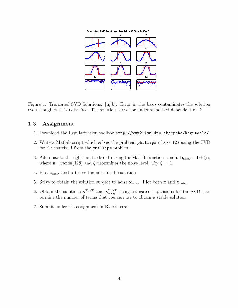
Figure 1: Truncated SVD Solutions: |uTi b|. Error in the basis contaminates the solutioneven though data is noise free. The solution is over or under smoothed dependent on k

1.3 Assignment

1. Download the Regularization toolbox http://www2.imm.dtu.dk/~pcha/Regutools/

2. Write a Matlab script which solves the problem phillips of size 128 using the SVDfor the matrix A from the phillips problem.

3. Add noise to the right hand side data using the Matlab function randn: bnoisy = b+ζn,where n =randn(128) and ζ determines the noise level. Try ζ = .1.

4. Plot bnoisy and b to see the noise in the solution

5. Solve to obtain the solution subject to noise xnoisy. Plot both x and xnoisy.

6. Obtain the solutions xTSVD and xTSVDnoisy using truncated expansions for the SVD. De-

termine the number of terms that you can use to obtain a stable solution.

7. Submit under the assignment in Blackboard

4

2 Ill-Posed Problems January 21, 2014

Consider the mapping A which takes the solution f to output data g. Af = g. Inverseproblem: find f given g and A.

Definition 1 (Well-Posed). The problem of finding f from g is called well-posed (by Hadamardin 1923) if all

Existence a solution exists for any data g in data space,

Uniqueness the solution f is unique

Stability continuous dependence of f on g : the inverse mapping g → f is continuous.

The first two conditions are equivalent to saying that the operator A has a well definedinverse A−1.

Suppose there exists f1 such that Af1 = 0, then Af = g and Af(f + f1) = g so f is notunique.

Moreover, we require that the domain of A−1 is all of data space.

Definition 2 (Ill-Posed: according to Hadamard). A problem is ill-posed if it does not satisfyall three conditions for well-posedness.

Alternatively an ill-posed problem is one in which

1. g /∈ range(A)

2. inverse is not unique because more than one image is mapped to the same data, or

3. an arbitrarily small change in the data can cause an arbitrarily large change in theimage.

Example for a Discrete problem - do we know if a solution is good

Consider the linear system

A =

0.16 0.100.17 0.112.02 1.29

,b =

0.260.283.31

, x =

(11

)The least squares solution yields

xls = [7.0089,−8.3957]T ‖Axls − b‖2 = .00047, ‖x− xls‖2 = 124.38

Perturbing b by δb = [.01, .01, .001] yields

x′ls = [7.6946,−9.4674]T , ‖Ax′ls − b‖2 = .00048, ‖x− x′ls‖2 = 154.38

• A small residual does not imply a realistic solution

• Even without noise the ill-conditioning of A leads to a poor solution

• Perturbing b leads to a larger perturbation in x.

5

2.1 Singular Value Expansion (see Hansen Discrete Inverse prob-lems, Chapter 2)

Let L2([0, 1] × [0, 1]) be space of square integrable functions on [0, 1] × [0, 1], i.e. h ∈L2([0, 1]× [0, 1])

‖h‖22 =

∫ 1

0

∫ 1

0

h(s, t)2 ds dt is finite.

The Singular Value Expansion is

h(s, t) =∞∑i=1

µiui(s)vi(t)

• For the inner product < φ,ψ >=∫ 1

0φ(t)ψ(t)dt,

< ui, uj >=< vi, vj >= δ(i− j) orthonormality

• µi are the singular values of h, ordered from large to small

µ1 ≥ µ2 ≥ · · · ≥ 0.

2.1.1 Properties of the SVE

1. h(s, t) square integrable implies∑∞

i=1 µ2i must be bounded:

‖h‖2 =

∫ 1

0

∫ 1

0

(∞∑

i,j=1

µiµjui(s)uj(s)vi(t)vj(t)

)ds dt

=∞∑i=1

µ2i , by orthonormality of (vi(t), ui(s)).

For the sum to be bounded µi must decay faster than 1/√i.

2. Left and right singular functions of h(s, t) are (ui, vi):

• µ2i , ui of

∫ 1

0h(s, x)h(t, x)dx and

• µ2i , vi of

∫ 1

0h(x, s)h(x, t)dx.

<

∫ 1

0

h(s, x)h(t, x) dx, uk(s) > =<∑i,j

µiµjui(s)uj(t)

∫ 1

0

vi(x)vj(x) dx, uk(s) >

=<∑i

µ2iui(s)ui(t), uk(s) >= µ2

kuk(t).

We note

< vk(t),

∫ 1

0

h(x, t)h(x, s)dx > =< vk(t),

∫ 1

0

∑ij

µiµjvi(t)vj(s)(ui(x)uj(x)dx) >

=< vk(t),∑i

µ2i vi(t)vi(s) >=

∑i

µ2i vi(s) < vk(t), vi(t) >= µ2

kvk(s).

6

2.1.2 Properties of the Singular Functions

Basis for function Space ui and vi provide a basis for L2([0, 1]). If f, g ∈ L2([0, 1]) then

f(t) =∑i

< vi, f > vi(t) and g(s) =∑i

< ui, g > ui(s)

Fundamental Mapping vi to ui:∫ 1

0

h(s, t)vi(t)dt =

∫ 1

0

∞∑j=1

(µjuj(s)vj(t)) vi(t)dt

i.e. < h(s, t), vi(t) > = µiui(s), i = 1, 2, . . .

by the orthonormality of vi.

Smoothing of vi by kernel h(s, t) to give µiui.

The Integral Equation g(s) =∫ 1

0h(s, t)f(t) dt

Observe by the expansion for g and its relation to the integral equation that

∑i

< ui, g > ui(s) = g(s) =

∫ 1

0

∑j

µjuj(s)vj(t)

f(t) dt

=

∫ 1

0

∑ij

µjuj(s)vj(t) < vi, f > vi(t) dt =∑i

µi < vi, f > ui(s) (2)

i.e.∑i

< ui, g > ui(s) =∑i

µi < vi, f > ui(s) yields (3)

and f(t) =∑i

< vi, f > vi(t) (4)

• By Fundamental relation µiui(s) is smoothed vi.

• Hence comparing sums of f and g, g is smoother than f .

• Also, if µi = 0 we can only have solution f of the integral equation if component< ui, g > ui(s) is zero.

• For µi 6= 0, i = 1, 2, . . . with µi < vi, f >=< ui, g > (taking inner product with uj(s)on each side in (4)) yields

f(t) =∑i

< ui, g >

µivi(t)

7

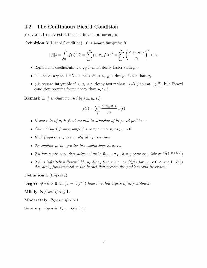
2.2 The Continuous Picard Condition

f ∈ L2([0, 1]) only exists if the infinite sum converges.

Definition 3 (Picard Condition). f is square integrable if

‖f‖22 =

∫ 1

0

f(t)2 dt =∞∑i=1

(< vi, f >)2 =∞∑i=1

(< ui, g >

µi

)2

<∞

• Right hand coefficients < ui, g > must decay faster than µi.

• It is necessary that ∃N s.t. ∀i > N , < ui, g > decays faster than µi.

• g is square integrable if < ui, g > decay faster than 1/√i (look at ‖g‖2), but Picard

condition requires faster decay than µi/√i.

Remark 1. f is characterised by (µi, ui, vi)

f(t) =∑i

< ui, g >

µivi(t)

• Decay rate of µi is fundamental to behavior of ill-posed problem.

• Calculating f from g amplifies components vi as µi → 0.

• High frequency vi are amplified by inversion.

• the smaller µi the greater the oscillations in ui, vi.

• if h has continuous derivatives of order 0, . . . , q µi decay approximately as O(i−(q+1/2))

• if h is infinitely differentiable µi decay faster, i.e. as O(ρi) for some 0 < ρ < 1. It isthis decay fundamental to the kernel that creates the problem with inversion.

Definition 4 (Ill-posed).

Degree if ∃α > 0 s.t. µi = O(i−α) then α is the degree of ill-posedness

Mildly ill-posed if α ≤ 1.

Moderately ill-posed if α > 1

Severely ill-posed if µi = O(e−αi).

8

Further Details

• Note in discussion we always assume that the equality signs with infinite sums implyuniform convergence for continuous functions. i.e. for solution of the integral equationthere exists N such that for all n > N∣∣∣∣∣f(t)−

n∑i=1

< ui, g >

µivi(t)

∣∣∣∣∣ < ε, ∀ t ∈ [0, 1]

• If the kernel is discontinuous convergence is with respect to the mean square,

‖f(t)−n∑i=1

< ui, g >

µivi(t)‖2 < ε, ∀ t ∈ [0, 1]

Example of an Ill-Posed Problem January 28, 2014

Consider the first kind Fredholm integral equation h(s, t),∫ 1

0

h(s, t)f(t)dt = g(s).

Consider functions fp fp = sin(2πpt), p = 1, 2, . . . . For arbitrary square integrable h,

gp =

∫ 1

0

h(s, t)sin(2πpt)dt→ 0 as p→∞.

As frequency of fp, amplitude of g decreases due to smoothing by h

This is a statement of the Riemann Lebesque Lemma (gp is smoother than fp)

Finding f from smoother g amplifies high frequencies in f .

Ratio fpgp

can become arbitrarily large for p large enough.

Problem is ill-posed because solution f is not continuously dependent on data g.

Non existence of a Solution : Ursell∫ 1

0

1

s+ t+ 1f(t) dt = 1, 0 ≤ s ≤ 1

Clearly h(s, t) = 1s+t+1

and g = 1.

Defining gk(s) =k∑i

< ui, g > ui(s) then

‖g − gk‖2 → 0 with k →∞ but

fk(t) =k∑i

< ui, gk >

µivi(t) satisfies‖fk‖2 →∞.

fk does not converge to a square integrable solution. (See reference for the plots)

9

2.2.1 Ambiguity in Inverse Problems: non unique solution

If the integral operator has a null space∫ 1

0

h(s, t)f(t) = 0, for some f(t)

then f is called an annihilator for h, as is αf for any scalar α.Null space of h is the space of all annihilators f . Moreover, by the fundamental relation

null(h) = spanvi|µi = 0

If there are only a finite number of µi > 0, the kernel is degenerate

Another example: degenerate kernel

Consider ∫ 1

−1

(s+ 2t)f(t) dt = g(s), −1 ≤ s ≤ 1.

It is possible to find the solution. We set h(s, t) =∑

i µiui(s)vi(t) and solve for the constantsunder assumptions that we have both constant and first order polynomial terms for the basisfunctions, with normalization. We find

u1(s) = 1/√

2 u2(s) =√

3/√

2s v1(t) =√

3/√

2t v2(t) = 1/√

2

µ2 = 2/√

3 µ1 = 4/√

3 µi = 0, i > 2

A solution exists only if

g ∈ range(h) = spanu1, u2 implies

g = a+ bs f =b

4+

3

2at

But notice that f = 3t2 − 1 is an annihilator and hence f is not unique!

2.2.2 Spectral Properties of the Singular Functions: Brief Overview

Define the integral operator

[Hf ](s) =

∫ π

−πh(s, t)f(t) dt and assume

1. h is real and continuous on [−π, π]× [−π, π].

2. for simplicity ‖h(π, t)− h(−π, t)‖2 = 0.

3. h is square integrable with singular set (µi, ui, vi) such that

[Hvj](s) = µjuj(s), [H∗uj](t) = µjvj(t)

10

An analysis can be performed to demonstrate thatSingular functions are similar to Fourier functions : for small j, the large singular values

and corresponding singular functions correspond to low Fourier frequencies, but for large j(small singular values) correspond to the high frequencies

i.e. the singular functions are similar to trigonometric functions which explains theincreasing oscillations for the smaller singular values.

2.3 Noise in the data: for the SVE

Suppose that g is measured and contaminated by errors g = gexact + η where

gexact ∈ range(h) with ‖η‖2 ‖gexact‖2

Immediately from the SVE

f = fexact +∞∑i=1

< ui, η >

µivi(t)

where the second term is the contribution due to the noise.

• Noise is typically high frequency and we cannot anticipate η to satisfy the Picardcondition.

• Thus g /∈ range(h).

• Using the infinite sum for obtaining f is unlikely to yield a useful estimate of fexact

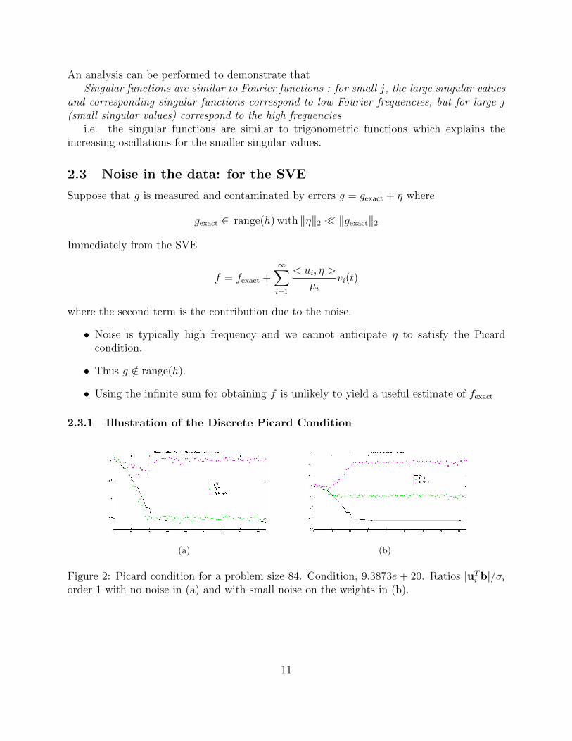
2.3.1 Illustration of the Discrete Picard Condition

(a) (b)

Figure 2: Picard condition for a problem size 84. Condition, 9.3873e+ 20. Ratios |uTi b|/σiorder 1 with no noise in (a) and with small noise on the weights in (b).

11

10 20 30 40 50 60

10−20

10−15

10−10

10−5

100

i

Picard plot

σi

|ui

Tb|

|ui

Tb|/σ

i

(a) Picard Plot for A1

10 20 30 40 50 60

10−15

10−10

10−5

100

i

Picard plot

σi

|ui

Tb|

|ui

Tb|/σ

i

(b) Picard Plot for A2

10 20 30 40 50 60

10−15

10−10

10−5

100

i

Picard plot

σi

|ui

Tb|

|ui

Tb|/σ

i

(c) Picard Plot for A3

Figure 3: In 3(a)-3(c) we illustrate the Picard condition for perfect data. The singular valueslevel out at a noise level of about 10−16 and 10−15 in panels 3(a) and 3(b)-3(c), respectively.One can see that addition of noise will then lead to a violation of the Picard condition

Summary

1. First kind Fredholm integral equation provides a linear model for inverse problemanalysis

2. For such models the solutions may be arbitrarily sensitive to perturbations of the data.

3. The SVE provides a means to analyse stability and existence of solutions.

4. Picard condition is necessary for existence of solution which is square integrable.

5. Right hand side g must be sufficiently smooth as measured by its SVE coefficients.

6. For more general inverse problems, e.g. Laplace transform, the operator is not compact,but a similar analysis for continuum of singular values can be applied.

3 Connecting the Continuous and the Discrete: Sys-

tem of Equations

3.1 Quadrature

Quadrature - how do we obtain A

Need to understand how we go from integral to matrix.

Integral Equation < h, f > = gDiscrete Form Ax = b

12

Quadrature to evaluate the integral (finite range [a, b]→ [0, 1])∫ 1

0

p(t)dt =n∑j=1

ωjp(tj) + En(p)

• En is the error which depends on n and the function p.

• tj are the abscissae, ωj are weights for the rule.

For < h, f >= g, p(t) = h(s, t)f(t). Thus

n∑j=1

ωjh(si, tj)f(tj) = g(si) + En(si), i = 1 . . .m.

Notice error depends also on the collocation point si.

Linear Equations

Neglecting E and setting x as the approximation to x we obtain

n∑j=1

ωjh(si, tj)xj = g(si), i = 1 . . .m.

Thus defining A = HD, where

• D is a diagonal matrix djj = ωj

• Hij = h(si, tj)

Ax = b

We could solve for scaled x say x = D−1x. Note this is right preconditioning.

Given b(m) i.e. of length m we obtain x(n) of length n.

What do we use for the weights ωj and abscissae tj?

Trapezium rule etc, are collocation based methods. Give values of f at discrete tj.

Expansion methods provide an expression for f(t).

13

Expansion Methods

Galerkin Approach

To relate the continuous and discrete we apply the expansion idea for the SVD.

SVE expands f and g in terms of basis functions and coefficients gi, fj.

g(m) ∈ spanψ1(s), ψ2(s), . . . , ψm(s) f (n) ∈ spanφ1(s), φ2(s), . . . , φn(s)

g(m)(s) =m∑i=1

giψi(s), f (n)(t) =n∑j=1

fjφj(t) integrate

g(s) =

∫ 1

0

h(s, t)f(t)dt ≈∫ 1

0

h(s, t)n∑j=1

fjφj(t)dt := θ(s)

g(s)−θ(s) is the residual. Galerkin approach require θ(s)−g(s) orthogonal to spanψ1(s), . . . , ψm(s)

< ψi(s), θ(s)− g(s) >= 0 i = 1 . . .m

Hence < ψi, θ >=< ψi, g > i = 1 . . .m gives

bi =< ψi, g >=

∫ 1

0

ψi(s)g(s)ds =< ψi, θ >=n∑j=1

fj < ψi(s),

∫ 1

0

h(s, t)φj(t)dt >

=n∑j=1

(∫ 1

0

∫ 1

0

h(s, t)ψi(s)φj(t)dsdt

)fj =

∑ij

Aijfj.

Expansion Quadrature Formula

The integration defines A and right hand side b by

Aij =

∫ 1

0

∫ 1

0

h(s, t)ψi(s)φj(t)dsdt, bi =< ψi, g >

Requires numerical quadrature for∫ 1

0

∫ 1

0

h(s, t)ψi(s)φj(t)dsdt ∀(i, j), bi =

∫ 1

0

ψi(s)g(s)ds, ∀i

If h(s, t) is symmetric h(s, t) = h(t, s); use φi(s) = ψi(s). Then A is symmetric.

14

Consider the case φi = ψi = ρi where ρi is the top hat

ρi(t) =

1√∆t

t ∈ [(i− 1)∆t, i∆t]

0 otherwise

Aij =1

h

∫ i∆t

(i−1)∆t

∫ jh

(j−1)∆t

h(s, t)dsdt bi =1√∆t

∫ i∆t

(i−1)∆t

g(s)ds

Sampling

g is sampled at si, thus

g(si) =

∫ 1

0

δ(s− si)g(s)ds suggestsψi(s) = δ(s− si) and

Aij =

∫ 1

0

∫ 1

0

h(s, t)δ(s− si)φj(t)dsdt =

∫ 1

0

h(si, t)φj(t)dt

so that the quadrature is reduced to one dimensional.

Sampling can also be implemented with the top hat and then

Aij =1√∆t

∫ 1

0

φj(t)

(∫ i∆t

(i−1)∆t

h(s, t)ds

)dt, bi =

∫ i∆s

(i−1)∆s

g(s)ds =√

∆sg(si).

3.2 Relationship of the Discrete SVD and Continuous SVE (forreal kernels and data)

SVD and SVE for square integrable kernel Hansen 1988

Idea : calculate an approximate SVE numerically via the SVD.

Given the SVD how are the relevant components uj, vj (columns of U and V )) and σj relatedto SVE basis functions ui(s), vi(t), singular values µi.

Discrete matrix A depends on ψi, i = 1, . . .m and φj, j = 1 . . . n.

Continuous kernel h depends on ψi, φj, (i, j) = 1 . . .∞.

Consider the approximate kernel h which is obtained by using the discrete set ψi, i = 1 . . . nand φj, j = 1 . . . n.

The result relates SVD of A to SVE of h

15

Singular Expansion of Degenerate Kernel

Suppose that matrix A is calculated using the expansion method with functions ψi, φj,i, j = 1, . . . n.

Calculate its SVD: Σ = diag(σi), U = (uij), V = (vij)

Let u(n)j (s) :=

∑ni=1 uijψi(s), v

(n)j (t) :=

∑ni=1 vijφi(t), j = 1 : n.

Theorem σ(n)j , u

(n)j , v

(n)j are exact singular values and functions of degenerate kernel

h(s, t) :=n∑i=1

n∑j=1

aijψi(s)φj(t)

i.e. we have SVE for an approximate kernel - how does that relate to the exact kernel?

h(s, t) =∑I

µiui(s)vi(t)

Limits with n, σ(n)j

SVD of A(n) = U (n)Σ(n)(V (n))T

Error of the kernel: δ2n := ‖h− h‖2 = ‖h‖2 − ‖A‖2

F

note ‖ · ‖2F is the Frobenious norm ‖A‖2

F =∑n

i,j=1 a2ij

Singular values converge σ(n)i ≤ σ

(n+1)i ≤ µi, i = 1, . . . , n.

Errors are bounded 0 ≤ µi − σ(n)i ≤ δn, i = 1, . . . , n.

Hence if δn → 0 with n increasing, approximate singular values converge uniformly to truesingular values.

SSE (Sum of squared error)∑n

i=1[µi − σ(n)i ]2 ≤ δ2

n.

Estimation of δn from ‖h‖2

Orthonormality u(n)i , v

(n)i are orthonormal. Convergence

max‖ui − u(n)i ‖, ‖vi − v

(n)i ‖ ≤ (

2δnµi − µi+1

)1/2

Practically observe that approximate singular values are more accurate than approximatesingular functions.

16

Significance of the Result

< u(n)j , g(n) > is important in the Picard condition.

< u(n)j , g(n) > =

∫ 1

0

(n∑i=1

u(n)ij ψi(s))(

n∑k=1

bkψk(s))ds

=∑i,k

u(n)ij bk < ψi, ψk >=

∑i

u(n)ij bi = uTj b

SVD and approximate inner products are related.

i.e. the exact inner products < uj, g >, i = 1, . . . , are approximated by < u(n)j , g(n) > which

is immediately obtained from the SVD for A.

Discrete Picard Condition Let τ denote the level such that ∀j > r, σj ≈ O(τ), dueto noise and rounding . The discrete Picard condition is satisfied if for j ≤ r thecoefficients |(u(n)

j )Tb| decay faster than σj.

Picard condition applies only for σj > O(τ). It is a condition on the size of the inner products

(u(n)j )Tb for j ≤ r.

Discrete Solution approximates Continuous Solution

SVE Solution SVD Solution

f(t) =∑

j<uj ,g>

µjvj(t) x =

∑nj=1

<u(n)j ,b>

σjv

(n)j

But < u(n)j ,b >=< u

(n)j , g(n) > where u

(n)j tends to uj with increasing n, while σ

(n)j converges

to µj with n.

Equivalently, if the discretization with increasing n is sufficiently good, the approximatesolution obtained from the SVD is essentially independent of the discretization.

For solving the first kind Fredholm integral equation numerically, the coefficients (u(n)j )Tb

and singular values σj reveal important information about the true quantities < uj, g > andµj.

Summary Approach - see Hansen for more details/examples

For increasing n until converged

1. Choose the orthonormal basis functions ψi(s) and φi(t).

2. Calculate matrix A with entries aij =< h(si, t), φj(t) >, i, j = 1, . . . , n.

17

3. Compute SVD of A

4. Estimate the singular functions uj(s) and vj(t)

Test Convergence of set of singular values.

End For

Is square integrable required for the theory?

Consider solving for f from the Laplace transform

g(s) =

∫ ∞0

e−stf(t)dt

Kernel e−st is not square integrable:∫ a

0

(e(−st))2ds =

∫ a

0

e−2stds =1− e−2ta

2t→ 1

2tfor a→∞

But∫∞

0t−1 is infinite,

∫∞0

∫∞0

(e(−st))2dsdt is infinite. No SVE

Now f(t) bounded for t→∞ implies g(s) is bounded ∀s ≥ 0.

Truncation for large a in Laplace transform introduces small error in g, and g decays withs. We obtain integral equation∫ a

0

e−stf(t)dt = g(s), 0 ≤ s ≤ a.

Now the kernel is square integrable.

Pick a and increase n, the SVD converges.

Pick n and increase a, the SVD does not converge. Demonstrates the lack of SVE for theLaplace Transform.

On the other hand, we can see convergence when the domain is not infinite!

Note that the analysis is totally determined by the kernel. But you can look at the coefficientsfor the expansion in g by picking a function with known Laplace transform!

18

4 The Discrete Solution with the SVD Feb 3, 2014

The thin SVD Solution

Consider general overdetermined discrete problem

Ax = b, A ∈ Rm×n, b ∈ Rm, x ∈ Rn, m ≥ n.

Thin singular value decomposition (SVD) of rectangular A is

A = UΣV T =n∑i=1

uiσivTi , Σ = diag(σ1, . . . , σn).

U of size m× n, V and Σ square of size n:

U = [u1, . . . ,un], V = [v1, . . . ,vn], σ1 ≥ σ2 ≥ σn ≥ 0

Orthonormal columns in U and V , left and right singular vectors for A

uTi uj = vTi vj = δ(i− j)→ UTU = V TV = V V T = In.

If A has full column rank σn > 0

A† = V Σ−1UT = A−1, m = n.

Moore Penrose Generalized Inverse

1. AA†A = A

2. A†AA† = A†

3. (AA†)∗ = AA†

4. (A†A)∗ = A†A

Expansion Solution

1. We can write x = V V Tx =∑n

i=1(vTi x)vi and

Ax =n∑i=1

(vTi x)Avi

2. But Avi = UΣV Tvi = UΣei = σiui . Thus

Ax =n∑i=1

σi(vTi x)ui

19

3. Similarly, for m = n, b =∑n

i=1(uTi b)ui.

4. Immediately compare coefficients and obtain σi(vTi x) = uTi b, i = 1, . . . , n and

x =n∑i=1

(uTi b)

σivi

5. Sensitivity of solutions depends on cond(A) = σ1/σn

Full SVD: Rectangular A

• Let U = [U1, U2] be square of size m, Σ rectangular of size m× n:

A = UΣV T = [U1, U2]

(Σ0

)V T

• The inverse is replaced by the pseudo inverse: if A has rank r

A† =r∑i=1

1

σiviu

Ti

• Solution of the LS problem is given by

x =r∑i=1

(uTi b)

σivi

• Sensitivity of solution depends on the condition as measured by σ1/σr.

• Recall singular values relation to eigenvalues λi of ATA, σ2i = λi

4.1 Filtering and Regularization (February 3, 2014)

4.2 Solution for Noisy Data

• Denote noise by n

• Spectral decomposition acts on the noise term in the same way it acts on the exactright hand side b. e.g.

x =r∑i=1

(uTi (bexact + n)

σi)vi = xexact +

r∑i=1

(uTi n

σi)vi

• If n is uniform, anticipate |uTi n| of similar magnitude ∀i.

20

• Can only recover components that arise from |uTi b| greater than the noise level.

• But anticipate σi → 0. σi small represents high frequency component in the sense thatui, vi have more sign changes as i increases.

• (uTi n

σi) is the coefficient of vi in the error image.

• If 1/σi large the contribution of the high frequency error is magnified due to (uTi n

σi).

Estimating rank of A for implementing the TSVD

• Results suggest that we need information on SVD of A

• Also need information on the spread of the singular values.

• Ideally information on the noise level in the data is available.

• Practically we need the numerical rank of A.

• Practically it is not always viable to find the effective numerical rank

• We turn to other methods to find acceptable solutions.

4.3 The Filtered SVD - more general than truncation

The truncated SVD is a special case of spectral filtering

Recall x = A†b = V Σ†UTb.

The filtered solution is given by

xfilt =r∑i=1

γi(uTi b

σi)vi = V Σ†filtU

Tb, Σ†filt := diag(γiσi, 0m−r)

i.ex = V ΓΣ†UTb,

where Γ is the diagonal matrix with entries γi.

Notice again the relationship with the SVE - filter out the terms which are noise contami-nated.

γi ≈ 1 for large σi, γi ≈ 0 for small σi

Spectral filtering is used to filter the components in the spectral basis, such that noise insignal is damped.

How to chose filter factors γi?

Truncated SVD takes γi = 1, 1 ≤ i ≤ k and 0 otherwise to obtain solution xk.

21

4.4 Tikhonov Regularization - Filtering

Consider general overdetermined discrete problem

Ax = b, A ∈ Rm×n, b ∈ Rm, x ∈ Rn, m ≥ n.

Fit to data functional of the least squares problem is ‖Ax− b‖22

Define xLS = arg minx‖Ax− b‖2 and x by Ax = b, i.e. b ∈ Range(A)

We know that xLS is noise contaminated if A is ill-conditioned.

Add a penalty term with regularization parameter λ > 0

xλ = arg minx‖Ax− b‖2 + λ2‖x‖2

Regularized solution trades of ‖xλ‖2 against ‖b− Axλ‖2.

For small λ the fit to data term is more closely enforced and the solution may be noisy

For larger λ the regularization term is enforced and so the solution is smoothed.

(a) (b) (c)

Figure 4: In (a) example: noise in b is n ∼ N(0, 10−7) (normally distributed, mean 0 andvariance 10−7)

22

Solution for Different Choices of λ

(a) (b) (c)

(d) (e) (f)

(g) (h) (i)

(j) (k) (l)

Figure 5: Solutions x(λ)

23

Signal to Noise Ratio for Different Choices of λ

(a) (b) (c)

(d) (e) (f)

(g) (h) (i)

(j) (k) (l)

Figure 6: The Signal to Noise Ratio of the solution 10 log10 ‖x‖/‖x− x(λ)‖, true solutionx. Note of course this can’t be calculated for practical data

24

4.5 Investigating the Regularized solution

xλ = arg minx‖Ax− b‖2 + λ2‖x‖2

has equivalent formulation

xλ = arg minx

∥∥∥∥( AλIn

)x−

(b0n

)∥∥∥∥2

We need to know how to find λ: We can use the heuristic based on the L-Curve: Plotregularization term against the fidelity term for λ

log(‖xλ‖), log(‖Axλ − b‖)

Figure 7: On the left a corner and on the right no corner. The L-curve is expensive for generalmatrices A, but is very general and straightforward. It does not consider any informationon the noise structure

4.6 Properties of the regularized solution

Normal equations Theoretically the solution solves the equations which are obtained bytaking the derivative with respect to x Make sure you can prove this!

(ATA+ λ2I)xλ = ATb

It follows immediately from the equivalent formulation:

xλ = arg minx

∥∥∥∥( AλIn

)x−

(b0n

)∥∥∥∥2

Regularization matrix

xλ = R(λ)b whereR(λ) = (ATA+ λ2I)−1AT

Matrix R is also sometimes referred to as the generalized inverse or regularized inverse.Denoted by A] in Vogel.

25

Model error (not computable)

e(λ) = x− xλ = x−R(λ)(b)

= x−R(λ)(b + n) = x−R(λ)Ax−R(λ)n

= − (R(λ)A− In)x︸ ︷︷ ︸−R(λ)n︸ ︷︷ ︸= bias variance

= (In − V ΓV T )x− V ΓΣ†UTn

Note that exact values x and b not available and thus we investigate the solutionthrough known computable quantities.

Bias is the loss of information introduced by regularization - also called the Regularizationerror

Express x = V V T x and rewrite (In − V ΓV T )x then

(In − V ΓV T )x = V (In − Γ)V T x =n∑i=1

(1− γi)(vTi x)vi

=

∑ni=k+1(vTi x)vi → 0 as k → n ΓTSVD = diag(Ik, 0n−k)∑ni=1

λ2

σ2i+λ2

(vTi x)vi → 0 asλ→ 0 ΓTIK = diag(γi), γi =σ2i

σ2i+λ2

Now for both Tikhonov and TSVD we observe the form for Γ leads to the filtering ofthe bias. It is the error due to using Γ = Σfilt in place of Σ.

Variance is the amplification of the noise in the error and also tends to zero by appropriatechoice of λ. It is also called the perturbation error and is the inverted and filterednoise, consistently zero if Γ = 0. First express the variance of solving for right handside with noise n as a sum

V ΓΣ†UTn =n∑i=1

(uTi n)γiσi

vi =n∑i=1

(uTi n)σ2i

(λ2 + σ2i )σi

vi

Suppose in TSVD k is chosen by a threshold so that for i ≤ k γi/σi ≤ 1/λ, then equivalentwe assume for i > k γi/σi = 0 ≤ 1/λ.

For the Tikhonov filter observe γi/σi = (σ2i /(σ

2i + λ2))/σi = (σi + λ2/σi)

−1

• For σ2i > λ2, σi > λ and thus σi + λ2/σi > λ

• For σ2i ≤ λ2, 1/σi > 1/λ, so λ2/σi > λ and σi + λ2/σi > λ.

Hence in each case γi/σi = (σi + λ2/σi)−1 ≤ 1/λ and γi ≤ σi/λ for all i

26

Suppose that ‖n‖22 < δ2 then by orthogonality of columns of V

‖n∑i=1

(uTi n)γi/σivi‖2 =n∑i=1

|(uTi n)|2(γi/σi)2 < (δ/λ)2.

If λ = δp where p < 1 then as δ → 0 variance error goes to zero. Notice that we use‖UTn‖2 = ‖n‖2 for U orthogonal,

λ can be chosen so that the variance goes to zero for both TSVD and Tikhonov

4.6.1 Assignment Feb 4, 2014

This continues the phillips assignment from class using the Regularization toolbox.

1. Write a Matlab script which solves the problem phillips of size 128 using the SVDfor the matrix A from the phillips problem.

2. Add noise to the right hand side data using the Matlab function randn: bnoisy = b+ζn,where n =randn(128) and ζ determines the noise level. Try ζ = .1.

3. Explore n the solutions of the noisy problem : giving xTiknoisy(λ) for a range of λ.

4. Plot your own Lcurve for your solutions.

5. Find the corner of the L-curve and plot the optimal solution as compared to the exactsolution.

6. Look at the trace of the resolution matrix as a function of λ. Plot Trace against λ.Identify on your plot the optimal point as indicated by the L-curve analysis. What doyou observe?

A(λ) = AA] = A(ATA+ λ2I)−1AT

First derive an expression for the Trace ofA(λ) using the SVD for A. You can substitutethe expression in your m file using latex and publish.

7. Submit under the assignment in Blackboard

Review February 10, 2014

We review the notation and qualitative measures of the solution of the least squares problem

Regularization matrix R(λ) = (ATA+ λ2I)−1AT = V ΓΣ†UT and R(λ)A = V ΓV T

Filter Factors γi =σ2i

λ2+σ2i

all satisfy γi/σi ≤ λ.

Variance R(λ)n = V ΓΣ†UTn - amplification of noise in measurement error: called Per-turbation error.: already shown that λ can be chosen so that the variance goes tozero.

27

Solution x = V ΓΣ†UTb

Bias (In − R(λ)A)x = (In − V ΓV T )x - loss of information called Regularization error.We can estimate the bias using the expression for x and using the orthogonality of Vto write x = V V T x

‖(In − V ΓV T )x‖22 = ‖(In − Γ)V Tx‖2

2 = ‖(In − Γ)ΓΣ†UTb‖22

=n∑i=1

((1− γi)γiuTi b

σi)2 =

n∑i=1

λ2

σ2i + λ2

σ2i

σ2i + λ2

(uTi b

σi)2

We notice that the bias depends on products (1− γi)γi) with the weighted expansioncoefficients uTi b/σi.

• First |uTi b

σi| decays on average by Picard condition

• For small i (σi big) γi ≈ 1, and (1− γi)γi ≈ 0. Little error from large |uTi b

σi|

• For large i (1− γi) ≈ 1 and (1− γi)γi ≈ 0, also provides little damping of smaller

|uTi b

σi|

Indeed the choice of Γ controls size of the bias. For Tikhonov regularization we also have

γi =

1− ( λ

σi)2 +O(| λ

σi|4) σi λ

(σiλ

)2 +O(|σiλ|4) σi λ

Hence for λ ∈ [σr, σ1], γi ≈ 1 for small i, and γi ≈ (σi/λ)2 for large i (small σi)

Conclude Parameter λ controls the filtering. If λ ≈ γk, then filtered solution does notinclude components related to σk+1 . . . σr.

Moreover it is sensible to keep λ ∈ [σr, σ1].

4.7 How do we find λ?

First we introduce some measures of a solution”

Predictive error (not computable) requires e

p(λ) = Ae(λ) = Ax(λ)− Ax = AR(λ)b− b

Notice that it depends on the matrix AR(λ) := A(λ)

Define Influence Matrix or Resolution Matrix A(λ) = AR(λ).

A(λ) = AA] = A(ATA+ λ2I)−1AT

Regularized Residual or Predictive Risk is computable

p(λ) = Ax(λ)− Ax ≈ (Ax(λ)− b) = (A(λ)− Im)b := r(λ)

It can be used to estimate the error through the unbiased estimator:

28

4.7.1 Derivation of the Unbiased Predictive Risk for Estimating λ

Consider the predictive error - cannot be calculated

p(λ) = AR(λ)b− b = A(λ)(b + n)− b

= (A(λ)− Im)b︸ ︷︷ ︸+A(λ)n︸ ︷︷ ︸= deterministic stochastic

Consider the predictive risk - can be calculated

r(λ) = (A(λ)− Im)b

= (A(λ)− Im)b︸ ︷︷ ︸+ (A(λ)− Im)n︸ ︷︷ ︸= deterministic stochastic

Both expressions use the noise n.

Necessary Statistical Results

Mean-Variance Suppose random vector x has mean x0, covariance-variance matrix Σ.

• we say x ∼ (x0,Σ)

• Then measured b for the exact model b0 = Ax0, which is noise contaminated bynoise n with variance Cb of mean 0 satisfies b ∼ (Ax0, AΣAT + Cb)

Trace Operator is linear. trace(A + B) =trace(A)+trace(B) and trace(AT ) =trace(A).We note also the cyclic property trace(ABC) =trace(CAB), provided that dimensionsare consistent.

Definition 5 (Discrete White Noise Vector). A random vector n = (η1, η2, . . . , ηn) is adiscrete white noise vector provided that E(n) = 0 and cov(n) = σ2In. i.e.

E(ηi) = 0, E(ηiηj) = σ2δ2ij

σ2 is the variance of the white noise

Lemma 1 (Trace Lemma). Let y be deterministic and n a discrete white noise vector withvariance σ2. Then

E(‖y + An‖2) = ‖y‖2 + σ2trace(ATA)

29

Obtaining the Estimate

Use the Trace lemma and assume that the noise vector n is a discrete white noise vector.Estimate mean predictive error from E(‖p(λ)‖2) and E(‖r(λ‖2)

E(‖r(λ)‖2) = E(‖(A(λ)− Im)b + (A(λ)− Im)n‖2))

= ‖(A(λ)− Im)b‖2 + σ2trace((A(λ)− Im)T (A(λ)− Im)) and

E(‖p(λ)‖2) = E(‖(A(λ)− Im)b + A(λ)n‖2))

= ‖(A(λ)− Im)b‖2 + σ2trace(A(λ)TA(λ))

= E(‖r(λ)‖2) + σ2trace(A(λ)TA(λ))− σ2trace((A(λ)− Im)T (A(λ)− Im))

= E(‖r(λ)‖2) + σ2(2 trace(A(λ))−m) by linearity of trace

≈ ‖r(λ)‖2 + σ2(2 trace(A(λ))−m) := U(λ)

Notice that E(U(λ)) = E(‖p(λ)‖2) so that U is an unbiased estimator.

Thus seek λ such that U is minimum :

λ = arg minλ

(U(λ)).

An Example with UPRE

Figure 8: Notice the well-defined minimum. But requires the calculation of the trace

30

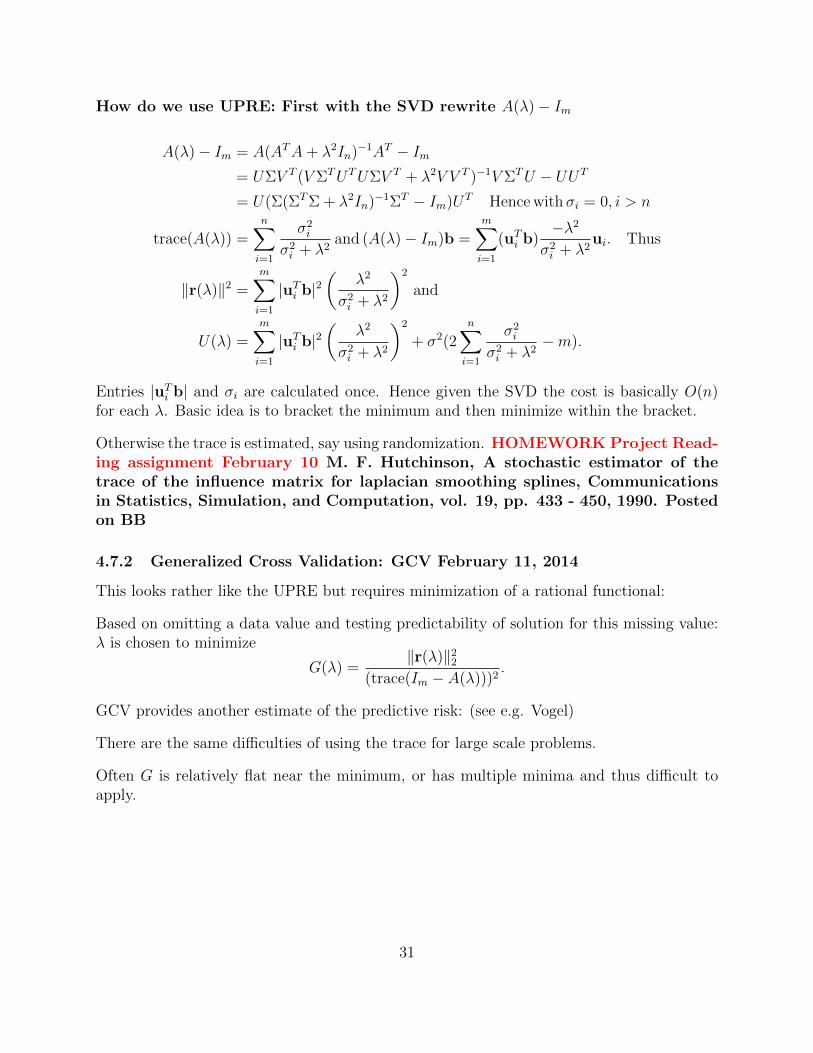
How do we use UPRE: First with the SVD rewrite A(λ)− Im

A(λ)− Im = A(ATA+ λ2In)−1AT − Im= UΣV T (V ΣTUTUΣV T + λ2V V T )−1V ΣTU − UUT

= U(Σ(ΣTΣ + λ2In)−1ΣT − Im)UT Hence withσi = 0, i > n

trace(A(λ)) =n∑i=1

σ2i

σ2i + λ2

and (A(λ)− Im)b =m∑i=1

(uTi b)−λ2

σ2i + λ2

ui. Thus

‖r(λ)‖2 =m∑i=1

|uTi b|2(

λ2

σ2i + λ2

)2

and

U(λ) =m∑i=1

|uTi b|2(

λ2

σ2i + λ2

)2

+ σ2(2n∑i=1

σ2i

σ2i + λ2

−m).

Entries |uTi b| and σi are calculated once. Hence given the SVD the cost is basically O(n)for each λ. Basic idea is to bracket the minimum and then minimize within the bracket.

Otherwise the trace is estimated, say using randomization. HOMEWORK Project Read-ing assignment February 10 M. F. Hutchinson, A stochastic estimator of thetrace of the influence matrix for laplacian smoothing splines, Communicationsin Statistics, Simulation, and Computation, vol. 19, pp. 433 - 450, 1990. Postedon BB

4.7.2 Generalized Cross Validation: GCV February 11, 2014

This looks rather like the UPRE but requires minimization of a rational functional:

Based on omitting a data value and testing predictability of solution for this missing value:λ is chosen to minimize

G(λ) =‖r(λ)‖2

2

(trace(Im − A(λ)))2.

GCV provides another estimate of the predictive risk: (see e.g. Vogel)

There are the same difficulties of using the trace for large scale problems.

Often G is relatively flat near the minimum, or has multiple minima and thus difficult toapply.

31

4.7.3 Why not just use r(λ) - rather than deal with the UPRE or GCV: Thediscrepancy principle

Calculate r(λ) = b− Ax(λ), noting that

b =∑i

(uTi b)ui Ax(λ) =m∑i=1

(σ2i )/(σ

2i + λ2)(uTi b)ui

r(λ) =m∑i=1

(λ2)/(σ2i + λ2)(uTi b)ui

Suppose that xλ ≈ x then r(λ) ≈ b− Ax = n ∈ Rm for b of length m.

Hence E( 1m‖Axλ − b‖2) ≈ E( 1

m‖Ax− b‖2) ≈ E( 1

m‖n‖2) = σ2, where n ∼ (0, σ2I).

Discrepancy Principle Find λ such that ‖r(λ)‖2 ≈ mσ2.

Is xλ ≈ x reasonable? Consider

F (λ) = ‖r(λ)‖2 =m∑i=1

(λ2/(σ2

i + λ2))2 |uTi b|2

Clearly F (λ) is continuous, F (0) = 0 and F (λ) → ‖b‖2 for λ → ∞. Hence there existsunique λ such that F (λ) = δ2, where δ = ‖n‖, provided δ < ‖b‖.

We note the regularized functional is given by

J(x) = ‖Ax− b‖2 + λ2‖x‖2

has solution xλ as argmin of the functional that satisfies for any other x

J(xλ) ≤ J(x)

32

Now take λ∗ such that F (λ∗) = δ2 and note

δ2 + λ2∗‖x(λ∗)‖2 = F (λ∗) + λ2

∗‖x(λ∗)‖2 = J(λ∗) ≤ J(x) = ‖Ax− b‖2 + λ2∗‖x‖2 =

‖Ax− b− n‖2 + λ2∗‖x‖2 = ‖n‖2 + λ2

∗‖x‖2 = δ2 + λ2∗‖x‖2

‖xλ‖2 ≤ ‖x‖2

i.e. the solution of that satisfies the discrepancy principle is necessarily smoother than themean solution (exact solution).

4.7.4 Some observations: Parameter Choice is Difficult

L-curve

• No unique solution(depends on find-ing the L)

• Requires multiplesolves to find ap-propriate range forthe corner

• Does not use noiselevel

• Easily justified.

Discrepancy

• Unique solution

• Direct solve usingNewton method

• Requires noise level

• Leads to a smoothedsolution

UPRE

• No unique solution

• Gives good esti-mates

• Requires noise level

• Minimizationrequired

• Needs trace esti-mator

GCV

• Multiple minima orflat

• Minimizationrequired

• Needs trace esti-mator

Assignment 4 Feb 11, 2014 Due Feb 18

This continues the phillips assignment from class using the Regularization toolbox.

1. Now that you have the Matlab script to solve the phillips problem using the L-curve you can easilymodify the script to compare the solution using

GCV

UPRE

Discrepancy principle

2. To obtain the solution by the GCV (UPRE) or the Discrepancy principle sweep through a range ofvalues for λ and pick the solution which minimizes the GCV (UPRE) functional and that finds theroot for the discrepancy principle.

3. Plot the relevant functionals, use subplot.

4. Plot the solutions obtained from the optimal λ.

5. Repeat for at least two noise levels.

6. Comment

7. Submit under the assignment in Blackboard

33

5 Interpretation: Rank and resolution February 18 2014

We need the following basic linear algebra result:

Theorem 5.1.

N(AT ) ⊥ R(A) (5)

N(AT ) + R(A) = Rm (6)

Proof. Suppose that y is any vector in the null space of the matrix AT : ATy = 0. ThusaTi y = yTai where ai is the ith column of A, i.e. y is perpendicular to all the columns ofA. But each ai = Aei is in the range of A and any element in the range of A is a linearcombination of these columns. Thus y is perpendicular to the range of A giving (5).

(6) is also immediate. In particular suppose that y ∈ Rm, then there is a unique decom-position y = z + x†, z ∈ N(AT ) and x† ∈ R(A).

5.1 The pseudo inverse solution of Ax ≈ b

We return to a brief discussion of the SVD for the solution of the problem

Ax ≈ b, A ∈ m× n, rank(A) = p ≤ minm,n (7)

A = UΣV T , Σ = [Σp, 0p×(n−p); 0(m−p)×n], Σp = diag(σ1, σ2, . . . , σp).

The terms of the SVD can be further expanded:

U = [ui] = [Up, U0]

V = [vi] = [Vp, V0]

from which we obtain by orthogonality

UTU = Im = [Up, U0]T [Up, U0] = [UTp ;UT

0 ][Up, U0] = diag(UTp Up, U

T0 U0) = diag(Ip, Im−p)

UUT = Im = [Up, U0][UTp ;UT

0 ] = UpUTp + U0U

T0 ,

with equivalent expressions for the orthogonal matrix V . Using the decomposition of U , Vthe SVD can be written in compact form

A = [Up, U0][Σp, 0p×(n−p); 0(m−p)×n][Vp, V0]

= UpΣpVTp .

Thus if b is a vector in the range of A, for some x

b = Ax = UpΣpVTp x = Up(ΣpV

Tp x) =

p∑i=1

uizi, z = ΣpVTp x,

34

and we see that any such b is a linear combination of the first p columns ui of U , so thatUp spans the range of A = R(A). Moreover, by Thm. 5.1 U0 spans N(AT ). Similarly, usingAT = VpΣpU

Tp , we obtain that the first p columns vi of V span the range of AT and V0 spans

N(A).From the compact form of the SVD we obtain

UpΣTp V

Tp x = b

V Tp x = Σ−1

p UTp b.

But x ∈ Rn which is spanned by N(A) + R(AT ) = span < vp+1, . . . ,vn > +span <v1, . . . ,vp >. Thus we may take x = V0α + Vpβ = z + x† for some vectors α, β, zand x†. Therefore

V Tp x = V T

p (V0α + Vpβ) = β = Σ−1p UT

p b

Vp(Σ−1p UT

p b) = Vpβ = x†

yielding x† as the pseudo inverse solution for the equations and defining the pseudo inverse

A† = VpΣ−1p UT

p .

Clearly the solution is nonuniquely given by

x = x† + z = (VpΣ−1p UT

p )b + z where z ∈ N(A). (8)

(8) leads to the following general conclusions about the solution of (7).

Square: m = n = p . The null spaces N(A) and N(AT ) are trivial. Moreover Vp = V ,Σp = Σ, Up = U and z = 0. Thus we obtain the solution of the square system ofequations

x = V Σ−1UTb = A†b.

Overdetermined full column rank p = n < m N(A) is trivial, z = 0 and x is uniquelydetermined as the solution of the normal equations :

(ATA)−1AT = (V ΣTUTUΣV T )−1(V ΣTUT ) = V (ΣTΣ)−1ΣTUT

= V (ΣTp Σp)

−1[ΣTp , 0][UT

p ;U0] = V Σ−1p UT

p = VpΣ−1p UT

p = A†

Underdetermined full row rank p = m < n N(AT ) is trivial, and UTp = U−1. Applying

A to x†

(UΣV T )(VpΣ−1p UT

p b) = UΣ[V Tp ;V T

0 ]VpΣ−1p U−1b

= UΣ[Ip; 0]Σ−1p U−1b = U [Σp, 0][Σ−1

p ; 0]U−1b

= U(Ip)U−1b = b.

35

Thus the pseudo inverse gives a solution x† which exactly fits the data, but is nonunique because any vector z ∈ N(A) can be added to the pseudo inverse solution x†.Consider the non unique solution x = z + x† then

‖x‖2 = ‖z‖2 + ‖x†‖2, because zTx† = 0

‖x‖2 ≥ ‖x†‖2 (9)

and x† is the solution of minimum length that satisfies the equations. Moreover,observe that

AT (AAT )−1 = (VpΣTpU

Tp )(UpΣpV

Tp VpΣ

TpU

Tp )−1

= VpΣTpU

T (UΣpΣTpU

T )−1 = VpΣTp (ΣpΣ

Tp )−1U−1

= VpΣ−1p U−1

p = A†,

from which we see that x† is given by

x† = AT (AAT )−1b = A†b

Loss of rank: p < minm,n. It is clear that both null spaces are now non trivial. Con-sider

Ax† = (UpΣpVTp )(VpΣ

−1p UT

p )b

= (UpUTp )b = bP (A)

where bP (A) denotes the projection of b onto R(A). Hence x† is a least squares solutionof (7). Moreover (8) sill applies and again as for (9) the solution has minimum length.

5.1.1 Properties of the pseudo-inverse solution

It is clear from the cases with loss of rank, p < minm,n or insufficient sampling p = m < n,the solution x† obtained is not a unique solution of the system of equations.

Solution covariance x† = A†b and thus when b ∼ (0, Cb), x† ∼ (0, A†Cb(A†)T ).

Cx† = A†Cb(A†)T = VpΣ−1p UT

p CbUpΣ−1p V T

p

Cb = σ2I Cx† = σ2VpΣ−1p Σ−1

p V Tp = σ2

p∑i=1

vivTi

σ2i

.

As i increases σi are smaller, contributions to the covariance are larger, and thus if wetruncate the solution we reduce its variance. i.e. the solution is smoother.

Bias Unless p = n the solution may have nonzero components due to projections on V0.Thus bias due to not using this information may be larger than that introduced bymeasurement error in b.

36

Model Resolution Suppose the true solution is x. Then b = Ax and we have the gener-alized inverse solution for the exact problem

x† = A†Ax = Rxx defining Rx = A†A (10)

the resolution matrix. Clearly Rx characterizes the effect of using the generalizedinverse solution:

Rx = VpΣ−1p UT

p UpΣpVTp = VpΣ

−1p ΣpV

Tp = VpV

Tp . (11)

(i) N(A) = 0, p = n and Rx = In. The original model x is recovered exactly in theabsence of noise. The resolution is perfect.

(ii) N(A) 6= 0, p = rank(A) < n and R is symmetric but not the identity. It is anindication of the smearing of the solution x†i 6= xi. The trace(Rx) is a measure of theresolution. If trace(Rx) ≈ n then Rx is close to the identity. For the expected value

E(x†) = E(A†b) = A†E(b) = A†Ax = Rxx.

Therefore the bias introduced is

E(x†)− x = (Rx − I)x = (VpVTp − In)x

‖E(x†)− x‖ ≤ ‖Rx − I‖ ‖x‖,

and we can deduce that the diagonal elements of the resolution matrix which are closeto 1 will yield elements of x which are resolved well. In contrast, small elements suggestpoorly resolved elements in x, significantly biased components.

Data Resolution Given a solution x it is also a question whether the data is well-resolved,

b ≈ Ax = AA†b = Rbb Rb = AA†

Rb = UpΣpVTp VpΣ

−1p UT

p = UpUTp = Im − U0U

T0 .

If N(AT ) = 0 then U0 = 0 and the data fit exactly, otherwise, p < m and the data arenot exactly reproduced.

Summary Note that the resolution matrices are independent of the data and hence ofnoise: they are dependent on the model matrix A. Solution depends on

Bias caused by limited resolution - determined by A - independent of noise.

Noise mapped from data to model.

Shaw order 0

http://math.la.asu.edu/~rosie/classes/Spring2013_files/rankdefhtml/regshaw.html We can alsoexamine the resolution due to rank regularization i.e. for the truncated examples. We look at some examplesfor an underdetermined matrix.

37

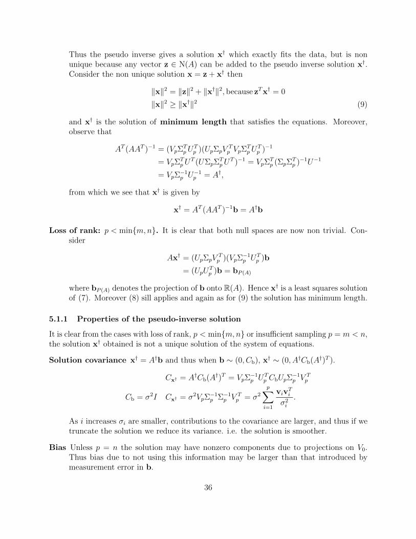
5.1.2 Example of Rank Reduction for APM 520: from Aster Borchers andThurber

Rosemary Renaut This is Example 3.1 in the book of straight ray path tomography The domain is of size 3x 3 measured at 8 points yielding an underdetermined system of equations

close all, clear all, clc

pos=get(0,’defaultfigureposition’);

A=zeros(8,9);row=[1 0 0 1 0 0 1 0 0];

A(1,:)=row;A(2,:)=[row(9) row(1:8)]; A(3,:)=[row(8:9) row(1:7)];

row=[1 1 1 0 0 0 0 0 0];

A(4,:)=row;A(5,:)=[row(7:9) row(1:6)]; A(6,:)=[row(4:9) row(1:3)];

A(7,1)=2^(1/2);A(7,5)=A(7,1);A(7,9)=A(7,1);A(8,9)=A(7,1);

figure(1), subplot(1,2,1),imagesc(A);colorbar;figprops,

title(’The Matrix ’);

[U,s,V]=svd(A);

% We see that the actual rank is not 8 but 7

subplot(2,1,2),semilogy(diag(s),’*’); figprops,

title(’Singular Values of A’);

Figure 9: Matrix and singular values

Rx=V(:,1:7)*V(:,1:7)’;Nx(:,1)=V(:,8);Nx(:,2)=V(:,9);

Rb=U(:,1:7)*U(:,1:7)’;Nb=U(:,8);

set(0,’defaultfigureposition’,[380 320 540 200])

figure(3),subplot(1,2,1),imagesc(Rx);colorbar,figprops,

title(’ Model Resolution R_ x ’),

figure(3),subplot(1,2,2),imagesc(Rb),colorbar,figprops,

title(’ Data Resolution R_ b ’)

38

Figure 10: model resolution matrix Rx = A†A = VpVTp and the data resolution matrix

Rb = AA† = UpUTp , p = 7

% Elements of null space for x - any multiple can be added to solution

figure(4),subplot(1,3,1),imagesc(reshape(Nx(:,1),3,3)),colorbar,figprops,

title(’ null space ’)

figure(4),subplot(1,3,2),imagesc(reshape(Nx(:,2),3,3)),colorbar,figprops,

title(’ null space ’)

figure(4), subplot(1,3,3), imagesc(reshape(diag(Rx),3,3));colorbar,figprops

title(’Diagonal of R_x’)

Figure 11: Null Space Vectors and The trace of Rx determines the resolution of x

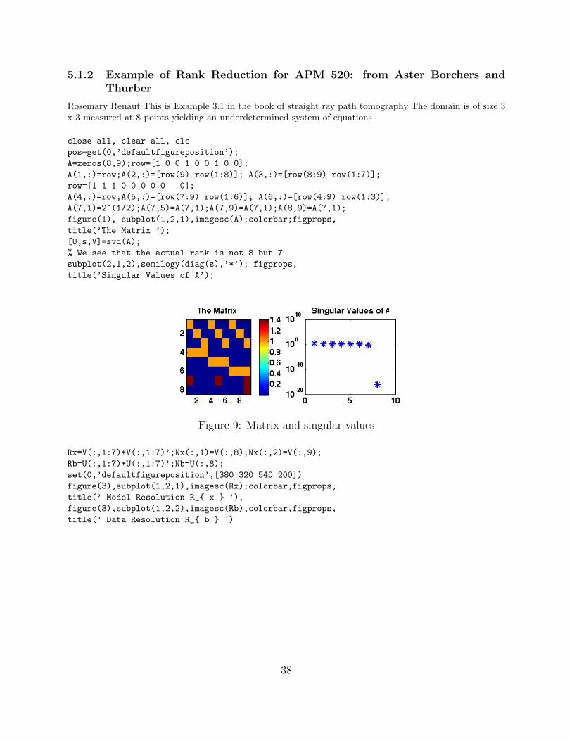
figure(5),subplot(1,2,1),imagesc(reshape([0 0 0 0 1 0 0 0 0],3,3));colorbar,

figprops,title(’Spike model ’)

subplot(1,2,2),imagesc(reshape(Rx(:,5),3,3));colorbar,figprops,

title(’Blurring of spike ’)

% Reset the figure position

set(0,’defaultfigureposition’,pos)

39

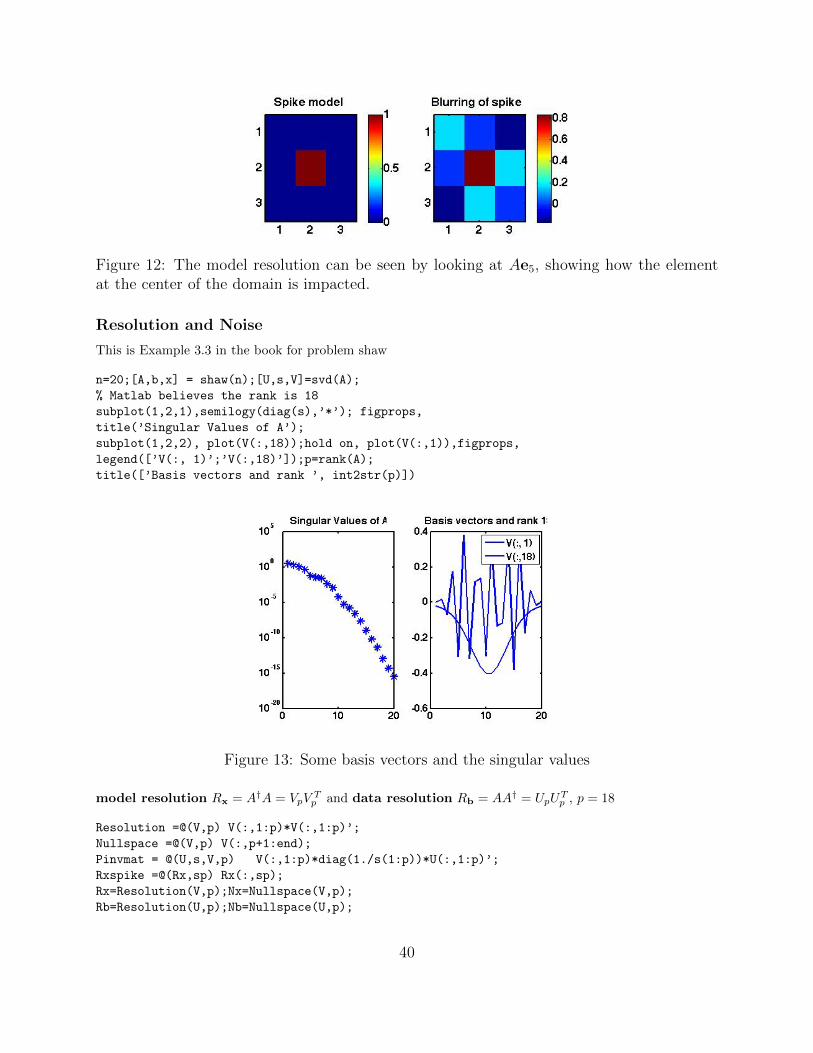
Figure 12: The model resolution can be seen by looking at Ae5, showing how the elementat the center of the domain is impacted.

Resolution and Noise

This is Example 3.3 in the book for problem shaw

n=20;[A,b,x] = shaw(n);[U,s,V]=svd(A);

% Matlab believes the rank is 18

subplot(1,2,1),semilogy(diag(s),’*’); figprops,

title(’Singular Values of A’);

subplot(1,2,2), plot(V(:,18));hold on, plot(V(:,1)),figprops,

legend([’V(:, 1)’;’V(:,18)’]);p=rank(A);

title([’Basis vectors and rank ’, int2str(p)])

Figure 13: Some basis vectors and the singular values

model resolution Rx = A†A = VpVTp and data resolution Rb = AA† = UpU

Tp , p = 18

Resolution =@(V,p) V(:,1:p)*V(:,1:p)’;

Nullspace =@(V,p) V(:,p+1:end);

Pinvmat = @(U,s,V,p) V(:,1:p)*diag(1./s(1:p))*U(:,1:p)’;

Rxspike =@(Rx,sp) Rx(:,sp);

Rx=Resolution(V,p);Nx=Nullspace(V,p);

Rb=Resolution(U,p);Nb=Nullspace(U,p);

40

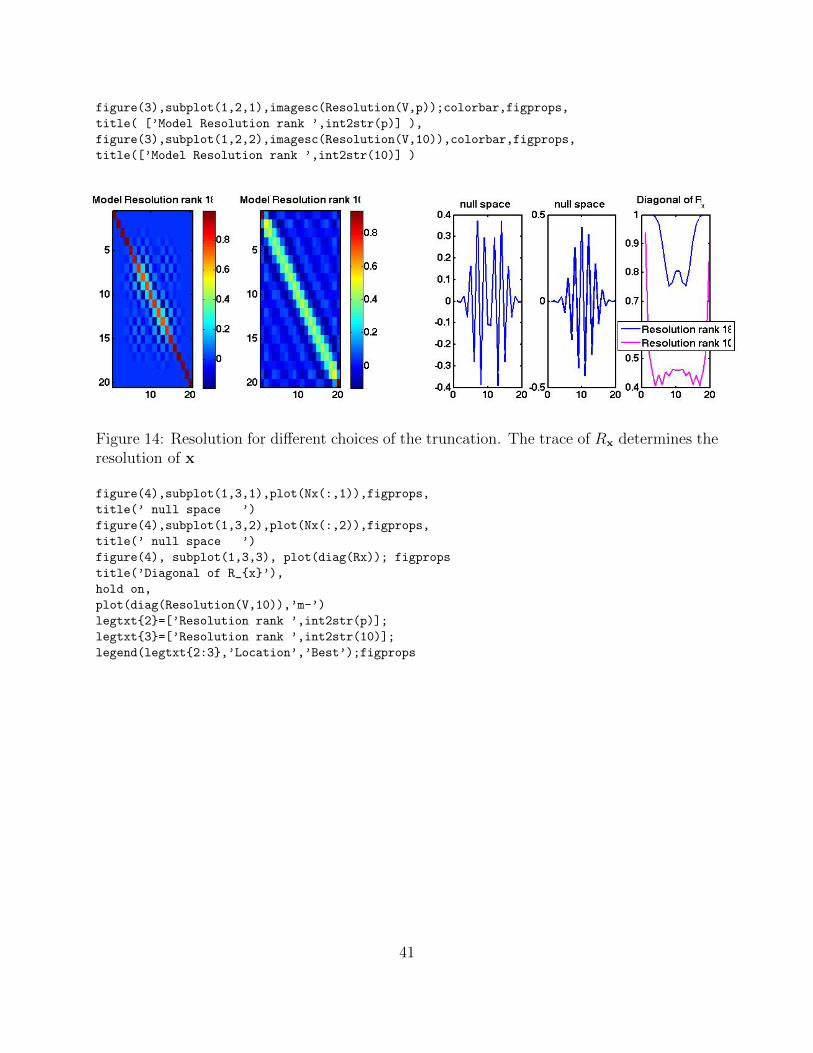
figure(3),subplot(1,2,1),imagesc(Resolution(V,p));colorbar,figprops,

title( [’Model Resolution rank ’,int2str(p)] ),

figure(3),subplot(1,2,2),imagesc(Resolution(V,10)),colorbar,figprops,

title([’Model Resolution rank ’,int2str(10)] )

Figure 14: Resolution for different choices of the truncation. The trace of Rx determines theresolution of x

figure(4),subplot(1,3,1),plot(Nx(:,1)),figprops,

title(’ null space ’)

figure(4),subplot(1,3,2),plot(Nx(:,2)),figprops,

title(’ null space ’)

figure(4), subplot(1,3,3), plot(diag(Rx)); figprops

title(’Diagonal of R_x’),

hold on,

plot(diag(Resolution(V,10)),’m-’)

legtxt2=[’Resolution rank ’,int2str(p)];

legtxt3=[’Resolution rank ’,int2str(10)];

legend(legtxt2:3,’Location’,’Best’);figprops

41

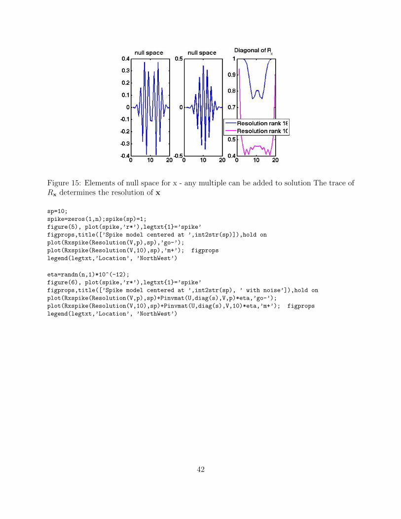
Figure 15: Elements of null space for x - any multiple can be added to solution The trace ofRx determines the resolution of x

sp=10;

spike=zeros(1,n);spike(sp)=1;

figure(5), plot(spike,’r*’),legtxt1=’spike’

figprops,title([’Spike model centered at ’,int2str(sp)]),hold on

plot(Rxspike(Resolution(V,p),sp),’go-’);

plot(Rxspike(Resolution(V,10),sp),’m+’); figprops

legend(legtxt,’Location’, ’NorthWest’)

eta=randn(n,1)*10^(-12);

figure(6), plot(spike,’r*’),legtxt1=’spike’

figprops,title([’Spike model centered at ’,int2str(sp), ’ with noise’]),hold on

plot(Rxspike(Resolution(V,p),sp)+Pinvmat(U,diag(s),V,p)*eta,’go-’);

plot(Rxspike(Resolution(V,10),sp)+Pinvmat(U,diag(s),V,10)*eta,’m+’); figprops

legend(legtxt,’Location’, ’NorthWest’)

42

Figure 16: The model resolution can be seen by looking at Rxe10, showing how a spikeis impacted. The model resolution under noise η in b: xnoisy = A†bnoisy = A†(b + η) =Rxb + A†η. Hence e10 goes to Rxe10 + A†η

Does increasing the sampling assist in such problems? Look at the following example which is withn = 100 as compared to n = 20 for problem shaw

http://math.la.asu.edu/~rosie/classes/Spring2013_files/rankdefhtml/rankdefshawbig.html

5.1.3 Resolution under Regularization

First of all we recognize that we can immediately write down the regularized resolution matrices using thedefinition of the regularized inverse

A†(λ) = (ATA+ λ2I)−1AT Rx(λ) = A†A Rb(λ) = AA† (12)

Rx(λ) = A(λ) = V ΓV T , Rb(λ) = UΓUT Γ = diag(γi) = diag(σ2i

σ2i + λ2

). (13)

and the filtering impacts the relevant resolution matrices.

5.1.4 Assignment Feb 18, 2014 Due Feb 20, 2014

1. Investigate the provided example for the resolution under truncation, i.e. regularization by truncation.

2. This one again continues the phillips assignment with regularization parameter estimation from classusing the Regularization toolbox.

(a) For the solutions that you have obtained for the ideal regularization parameters in each case,also now plot the resolution matrices Rx and Rb as another way to contrast the solutions.

(b) What can you observe as to the ability of the different methods to preserve the resolution ofthe model and the data?

(c) Investigate the impact on a pulse at the middle of the domain, en/2.

43

5.2 More on Regularization: February 19 2014

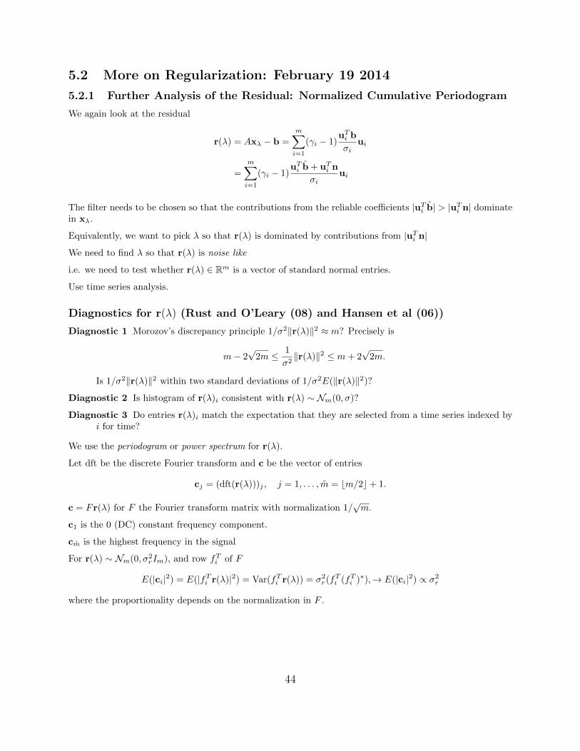
5.2.1 Further Analysis of the Residual: Normalized Cumulative Periodogram

We again look at the residual

r(λ) = Axλ − b =

m∑i=1

(γi − 1)uTi b

σiui

=

m∑i=1

(γi − 1)uTi b + uTi n

σiui

The filter needs to be chosen so that the contributions from the reliable coefficients |uTi b| > |uTi n| dominatein xλ.

Equivalently, we want to pick λ so that r(λ) is dominated by contributions from |uTi n|

We need to find λ so that r(λ) is noise like

i.e. we need to test whether r(λ) ∈ Rm is a vector of standard normal entries.

Use time series analysis.

Diagnostics for r(λ) (Rust and O’Leary (08) and Hansen et al (06))

Diagnostic 1 Morozov’s discrepancy principle 1/σ2‖r(λ)‖2 ≈ m? Precisely is

m− 2√

2m ≤ 1

σ2‖r(λ)‖2 ≤ m+ 2

√2m.

Is 1/σ2‖r(λ)‖2 within two standard deviations of 1/σ2E(‖r(λ)‖2)?

Diagnostic 2 Is histogram of r(λ)i consistent with r(λ) ∼ Nm(0, σ)?

Diagnostic 3 Do entries r(λ)i match the expectation that they are selected from a time series indexed byi for time?

We use the periodogram or power spectrum for r(λ).

Let dft be the discrete Fourier transform and c be the vector of entries

cj = (dft(r(λ)))j , j = 1, . . . , m = bm/2c+ 1.

c = Fr(λ) for F the Fourier transform matrix with normalization 1/√m.

c1 is the 0 (DC) constant frequency component.

cm is the highest frequency in the signal

For r(λ) ∼ Nm(0, σ2rIm), and row fTi of F

E(|ci|2) = E(|fTi r(λ)|2) = Var(fTi r(λ)) = σ2r(fTi (fTi )∗),→ E(|ci|2) ∝ σ2

r

where the proportionality depends on the normalization in F .

44

Normalized Cumulative Periodogram

Diagnostic 1 Parseval’s relation: ‖dft(r(λ))‖2 = ‖r(λ)‖2

Diagnostic 2 & 3 Normalized Cumulative Periodogram(NCP):

Calculate the ratio of the cumulative sum of entries

wj =

∑ji=1 |cj |2∑mi=1 |ci|2

, j = 1, . . . , m,

Because E(|ci|2) ∝ σ2r , for all i, the power spectrum is flat: wj ≈ 2j/m.

Define j = (j − 1)/(m− 1), 0 ≤ j ≤ .5.

Then (j,wj) is a straight line wj ≈ 2j of length√

5/2.

Ideally w = w, wj = 2j

For 5% significance level the NCP is within Kolmogorov Smirnoff limits ±1.35m−1/2

How to test automatically: various options - Hansen’s NCP test

Minimize the deviation from straight line λNCP = arg minλ ‖w(λ)− w‖2

(a) Deviation from Straight line with λ (b) NCP for some different λ

(c) Residual and Periodogram: λ (d) Augmented and periodogram: λ

Figure 17: Example NCP Comparing the Residual Periodogram and the Cumulative Resid-ual: Notice the reverse L for the deviation: hence the corner can be found.

45

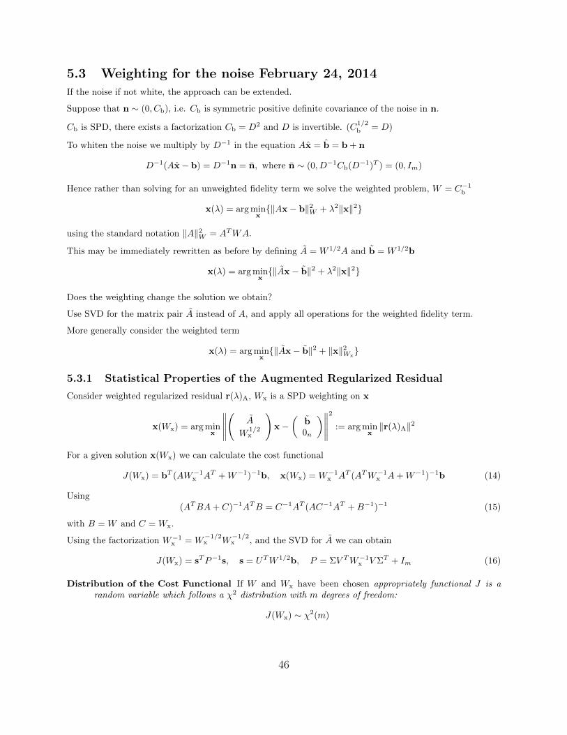
5.3 Weighting for the noise February 24, 2014

If the noise if not white, the approach can be extended.

Suppose that n ∼ (0, Cb), i.e. Cb is symmetric positive definite covariance of the noise in n.

Cb is SPD, there exists a factorization Cb = D2 and D is invertible. (C1/2b = D)

To whiten the noise we multiply by D−1 in the equation Ax = b = b + n

D−1(Ax− b) = D−1n = n, where n ∼ (0, D−1Cb(D−1)T ) = (0, Im)

Hence rather than solving for an unweighted fidelity term we solve the weighted problem, W = C−1b

x(λ) = arg minx‖Ax− b‖2W + λ2‖x‖2

using the standard notation ‖A‖2W = ATWA.

This may be immediately rewritten as before by defining A = W 1/2A and b = W 1/2b

x(λ) = arg minx‖Ax− b‖2 + λ2‖x‖2

Does the weighting change the solution we obtain?

Use SVD for the matrix pair A instead of A, and apply all operations for the weighted fidelity term.

More generally consider the weighted term

x(λ) = arg minx‖Ax− b‖2 + ‖x‖2Wx

5.3.1 Statistical Properties of the Augmented Regularized Residual

Consider weighted regularized residual r(λ)A, Wx is a SPD weighting on x

x(Wx) = arg minx

∥∥∥∥∥(

A

W1/2x

)x−

(b0n

)∥∥∥∥∥2

:= arg minx‖r(λ)A‖2

For a given solution x(Wx) we can calculate the cost functional

J(Wx) = bT (AW−1x AT +W−1)−1b, x(Wx) = W−1x AT (ATW−1x A+W−1)−1b (14)

Using(ATBA+ C)−1ATB = C−1AT (AC−1AT +B−1)−1 (15)

with B = W and C = Wx.

Using the factorization W−1x = W−1/2x W

−1/2x , and the SVD for A we can obtain

J(Wx) = sTP−1s, s = UTW 1/2b, P = ΣV TW−1x V ΣT + Im (16)

Distribution of the Cost Functional If W and Wx have been chosen appropriately functional J is arandom variable which follows a χ2 distribution with m degrees of freedom:

J(Wx) ∼ χ2(m)

46

This is proved by noting that (14) may be written as

J(Wx) = bT (ATW−1x A+W−1)−1b

= ‖b‖2Z Z = (ATW−1x A+W−1)−1.

Now by b ∼ (0, ATW−1x A+W−1) when n ∼ (0,W−1) and x ∼ (0,W−1x ), yields Z1/2b ∼ (0, Im). Thus J isa sum of standard normal variables which in the limit is a χ2 distribution with mean m.

Appropriate weighting makes noise on b and on model x white

Of course noise on x is unknown, but this determines a parameter choice rule for Wx = λ2I using theaugmented discrepancy.

5.3.2 χ2 method to find the parameter (Mead and Renaut)

Interval Find Wx = λ2I such that

m−√

2mzα/2 < bT (ATW−1x A+W−1)−1b < m+√

2mzα/2.

i.e. E(J(x(Wx))) = m and Var(J) = 2m.

Posterior Covariance on x Having found Wx the posterior inverse covariance matrix is

Wx = ATWA+Wx

Root finding Find σ2x = λ−2 such that

F (σx) = sTdiag(1

1 + σ2xσ

2i

)s−m = 0. (17)

Discrepancy Principle note the similarity

F (σx) = sTdiag(1

(1 + σ2xσ

2i )2

)s−m = 0.

Homework: Due Prove the identities (15), (16) and (17).

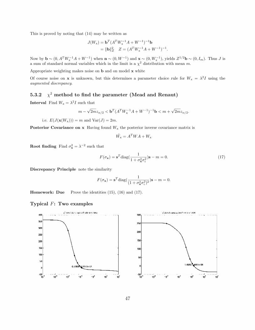
Typical F : Two examples

47

Newton’s method yields a unique solution (when one exists)

F is monotonically decreasing

No solution exists if asymptotically F > 0 as σ →∞ which implies no regularization is needed.

Likewise, F < 0 for all σx implies that the degrees of freedom is wrongly given, the noise on b was notcorrectly identified.

NCP for r(λ)A

The overall residual r(λ)A is also white noise like provided W is chosen appropriately. Thus, we can applyexactly the same NCP idea to this residual

(a) Deviation from Straight line with λ (b) NCP for some different λ

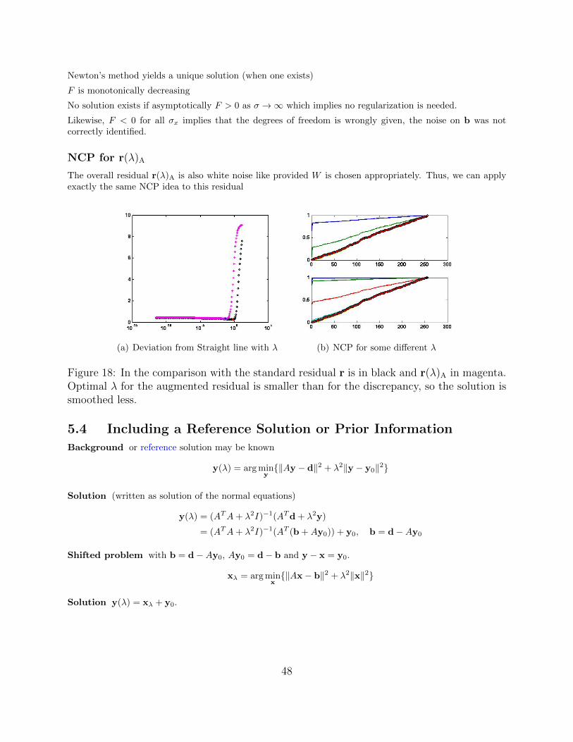
Figure 18: In the comparison with the standard residual r is in black and r(λ)A in magenta.Optimal λ for the augmented residual is smaller than for the discrepancy, so the solution issmoothed less.

5.4 Including a Reference Solution or Prior Information

Background or reference solution may be known

y(λ) = arg miny‖Ay − d‖2 + λ2‖y − y0‖2

Solution (written as solution of the normal equations)

y(λ) = (ATA+ λ2I)−1(ATd + λ2y)

= (ATA+ λ2I)−1(AT (b +Ay0)) + y0, b = d−Ay0

Shifted problem with b = d−Ay0, Ay0 = d− b and y − x = y0.

xλ = arg minx‖Ax− b‖2 + λ2‖x‖2

Solution y(λ) = xλ + y0.

48

5.5 Relating MAP and Tikhonov Regulariztion

Statistical interpretation of y0: Let p(x) be the probability for x and p(y|x) be the conditional probabilityof y given x

Maximum Likelihood Estimator (MLE) for obtaining parameter y given d is the parameter y whichmaximizes the likelihood function L(y) = p(d; y).

MLE maximizes the log likelihood l(y) = log p(d; y).

Example Suppose d is a realization of vector y ∼ N (y0, C).

Assume y0 is unknown. The probability density function is

p(y; y0, C) ∝ exp(−1

2(y − y0)TC−1(y − y0)) and

l(y) = −1

2(y − y0)TC−1(y − y0) + c,

where c is independent of y0, has maximizer y = y0.

Bayes Law If y and d are jointly distributed random vectors.

p(y|d) =p(d|y)p(y)

p(d)

MAP Maximum A Posteriori Estimator is the maximizer of p(y|d) with respect to y.

To obtain the MAP we use the linear model. Suppose y ∼ N (y0, Cy), n ∼ N (0, C) and d is a random vectordefined by the linear model Ay + n = d. Then d ∼ N (Ay, C) implies

p(d|y) ∝ exp(−1

2(d−Ay)TC−1(d−Ay)) and the prior is

p(y) ∝ exp(−1

2(y − y0)TC−1y (y − y0))

Combining terms and using Bayes Law the a posteriori log likelihood function is

l(y|d) = −1

2(d−Ay)TC−1(d−Ay)− 1

2(y − y0)TC−1y (y − y0) + c

where c is independent of y. Then the MAP estimator which maximizes l(y|d) is equivalent to the minimizerof the Tikhonov regularization

‖d−Ay‖2C−1 + ‖y − y0‖2C−1y

In this case y0 is the expected value of y.

5.6 Changing the basis by applying a different operator: March4, 2014

Imposing the regularization for the norm of x is not necessarily appropriate, dependent on what we anticipatefor the solution

Instead we consider the more general weighting ‖Lx‖2

This leads to the general problem

x(λ) = arg minx‖Ax− b‖2 + λ2‖Lx‖2

49

Suppose that L is invertible then we can solve for y = Lx noting for the normal equations

(ATA+ LTL)x = ATb

(ATAL−1 + LT )Lx = ATb

(ATAL−1 + LT )Lx = ATb

LT ((LT )−1ATAL−1 + In)Lx = ATb

(AT A+ In)y = ATb A = AL−1

and we see that this solves for the column scaled matrix A, with solution y = Lx, and x is found in adifferent basis.

However, typical L: L approximates the first or second order derivative

L1 =

−1 1. . .

. . .

−1 1

L2 =

1 −2 1. . .

. . .. . .

1 −2 1

L1 ∈ R(n−1)×n and L2 ∈ R(n−2)×n. Note that neither L1 nor L2 are invertible.

5.6.1 Boundary Conditions: Zero

Operators L1 and L2 provide approximations to derivatives

Dx(ui) ≈ ui+1 − ui Dxx(ui) ≈ ui+1 − 2ui + ui−1

Boundary is at u1 and un.

Suppose zero outside the domain u0 = un+1 = 0

Dx(un) = un+1 − un = −unDxx(u1) = u2 − 2u1 + u0 = u2 − 2u1

Dxx(un) = un+1 − 2un + un−1 = −2un + un−1

L01 =

−1 1

. . .. . .

−1 1−1

L02 =

−2 11 −2 1

. . .. . .

. . .

1 −2

L01, L

02 ∈ Rn×n. Both L1, L2 are invertible.

5.6.2 Boundary Conditions: Reflexive

Suppose reflexive outside the domain u0 = u2, un+1 = un−1

Dx(un) = un+1 − un = un−1 − unDxx(u1) = u2 − 2u1 + u0 = 2u2 − 2u1

Dxx(un) = un+1 − 2un + un−1 = −2un + 2un−1

LR1 =

−1 1

. . .. . .

−1 11 −1

LR2 =

−2 21 −2 1

. . .. . .

. . .

2 −2

50

LR1 , LR2 ∈ Rn×n. Neither L1, L2 invertible.

5.6.3 Boundary Conditions: Periodic

Suppose periodic outside the domain u0 = un, un+1 = u1

Dx(un) = un+1 − un = u1 − unDxx(u1) = u2 − 2u1 + u0 = un + 2u2 − u1Dxx(un) = un+1 − 2un + un−1 = u1 − 2un + un−1

LP1 =

−1 1 0

. . .. . .

−1 11 −1

LP2 =

−2 1 11 −2 1

. . .. . .

. . .

1 1 −2

LP1 , LP2 ∈ Rn×n. Neither L1, L2 invertible.

Both are circulant banded. We can use the FFT to form the matrix product.

5.6.4 The Generalized Singular Value Decomposition

Introduce generalization of the SVD to obtain a expansion for

x(λ) = arg minx‖Ax− b‖2 + λ2‖L(x− x0)‖2

Lemma 2 (GSVD). Assume invertibility and m ≥ n ≥ p. There exist unitary matrices U ∈ Rm×m,V ∈ Rp×p, and a nonsingular matrix X ∈ Rn×n such that

A = U

[Υ

0(m−n)×n

]XT , L = V [M, 0p×(n−p)]X

T ,

Υ = diag(υ1, . . . , υp, 1, . . . , 1) ∈ Rn×n, M = diag(µ1, . . . , µp) ∈ Rp×p,

with

0 ≤ υ1 ≤ · · · ≤ υp ≤ 1, 1 ≥ µ1 ≥ · · · ≥ µp > 0, υ2i + µ2i = 1, i = 1, . . . p.

Use Υ and M to denote the rectangular matrices containing Υ and M .

5.6.5 Solution of the Generalized Problem using the GSVD

As for the SVD we need the expression for the regularization matrix

R(λ) = (ATA+ λ2LTL)−1AT = (XT )−1(ΥT Υ + λ2MT M)−1ΥTUT

Notice(ΥT Υ + λ2MT M)−1ΥT = diag(diag(

νiν2i + λ2µ2

i

), 1, . . . , 1)

Thus

xλ =

p∑i=1

νiν2i + λ2µ2

i

(uTi b)xi +

n∑i=p+1

(uTi b)xi

51

where xi is the ith column of (XT )−1 With ρi = νi/µi we have

xλ =

p∑i=1

ρ2iνi(ρ2i + λ2)

(uTi b)xi +

n∑i=p+1

(uTi b)xi

=

p∑i=1

γiuTi b

νixi +

n∑i=p+1

(uTi b)xi, γi =ρ2i

ρ2i + λ2, i = 1, . . . , p.

Notice the similarity with the filtered SVD solution

xλ =

r∑i=1

γiuTi b

σivi, γi =

σ2i

σ2i + λ2

.

We can also immediately express the resolution matrix for the mapped regularization.1

A(λ) = X−TΓXT , γi =ρ2i

ρ2i + λ2. (18)

Shaw order 1

http://math.la.asu.edu/~rosie/classes/Spring2013_files/rankdefhtml/genregshaworder1.html

Shaw order 2

http://math.la.asu.edu/~rosie/classes/Spring2013_files/rankdefhtml/genregshaworder2.html

VSP order 1 and 2

http://math.la.asu.edu/~rosie/classes/Spring2013_files/rankdefhtml/genregvsp.html

5.6.6 Finding the optimal regularization parameter using the χ2 test

For the generalized Tikhonov regularization the degrees of freedom for the cost functionalare m− n+ p, L of size p× n.

Basic Newton iteration to solve F (σ) = 0,

y(σ(k)) is the current solution for which

x(σ(k)) = y(σ(k)) + x0

Use the derivative

J ′(σ) = − 2

σ3‖Lx(σ)‖2 < 0. (19)

and line search parameter α(k) to give

σ(k+1) = σ(k)(1 + α(k) 1

2(

σ(k)

‖Lx(σ(k))‖)2(J(σ(k))− (m− n+ p))). (20)

1Recall that we use the definition A = UΥXT , L = VMXT for the GSVD. The matlab functioncgsvd assumes A = UΥX−1, L = VMX−1 and returns [U, sm,X, V,W ] where sm(i, :) = [υi, µi] andW = X−1. Let our definition replace XT = ZT , A(λ) = Z−TΓZT . Then returned from cgsvd we obtainW = X−1 = ZT and X = (ZT )−1 = Z−T . Hence in the formula in terms of the returned entries from cgsvd

we have Rx = A(λ) = XΓW .

52

5.6.7 More on the Generalized Tikhonov Solutions

• The parameter estimation techniques extend for the solutions using the GSVD.

• As with the χ2 method, other regularization techniques can be extended without theGSVD

• Observation on the shifted solution: for the result with the χ2 we require that E(x) =x0. i.e we know the expected average solution. When this is not available we canmodify the approach for a non central χ2 distribution.

• For missing data Hansen notes that solution in the 2− norm leads to solutions whichhave x = 0 if there are missing data but replacing operator by L the first or sec-ond derivative operator fills in a solution which more appropriately fills in a realisticsolution.

5.6.8 An Observation on shifting and smoothing

Find the solution y which satisfies

y(λ) = arg miny‖Ay − d‖2 st ‖L(y − y0)‖2 is minimum (21)

Consider the decomposition V = [V1, V2] = [v1, . . . ,vk,vk+1, . . . ,vn], where we assume thatthe columns of V1, V2 span the effective range and null space of A.

Now use the decomposition to separate the solution into two pieces: y = yk + y =∑ki=1

(uTi d)

σivi + V2c such that yk minimizes the fidelity term.

We want y such that ‖L(y − y0)‖ is minimum. Equivalently recalling the definition A† =(ATA)−1AT and noting

‖L(y − y0)‖ = ‖L(yk − y0) + Ly‖ = ‖L(yk − y0) + LV c‖

Then the term is minimum for

c = −(LV2)†L(yk − y0).

yielding the solution

y = yk − V2(LV2)†L(yk − y0) = (I − V2(LV2)†L)yk + V2(LV2)†Ly0

Hence the solution of the shifted system obtained from this solution for y is given by

x = y − y0 = (I − V2(LV2)†L)(yk − y0)

53

On the other hand suppose that we solve the shifted system directly for x using the samedecomposition for V . We immediately obtain the solution by applying the result for findingy to that for finding x when x0 = 0.

x = (I − V2(LV2)†L)xk = (I − V2(LV2)†L)k∑i=1

(uTi b)

σivi

= (I − V2(LV2)†L)k∑i=1

(uTi (d− Ay0)

σivi

= (I − V2(LV2)†L)yk − (I − V2(LV2)†L)k∑i=1

(uTi (Ay0)

σivi

= (I − V2(LV2)†L)yk − (I − V2(LV2)†L)(V1VT

1 )y0

= y − V2(LV2)†Ly0 − (I − V2(LV2)†L)(V1VT

1 )y0

= y − y0 + (I − V2(LV2)†L(I − V1VT

1 )y0

= y − y0 + (I − V2(LV2)†L)(V2VT

2 )y0 6= y − y0.

i.e. the same solution is not obtained. Although, note that L = I has y = x.

It is important to be careful when shifting in the regularization.

5.6.9 Practical Solution Techniques

Are the bases discussed so far relevant for all problems: we will look first at problems inwhich alternative options arise due to the specifics of the kernel. Fourier and cosine bases.

For practical problems, i.e. of reasonable size, we do not use SVD or GSVD. Rather we useiterative methods - LSQR

Typically use iterative Krylov method with preconditioning

Goal to utilize forward operations for A and AT

We will also look at the randomized SVD

54

6 One Dimensional Problems March 24 2014

6.1 Continuous Problem

6.1.1 Zero Function Outside the Domain: Dirichlet Condition

We consider the integral equation

g(s) =

∫ π

0

h(s, t)f(t)dt.

When f(t) = 0 outside the interval [0, π] this completely defines the formulation. Supposethat s and t are discretized on the interval [0, π] by

si =(2i− 1)π

2mtj =

((2j − 1)π

2m∆s =

π

m= ∆t i, j = 1 : m

then the integral equation is approximated by the midpoint quadrature rule

g(si) ≈m∑j=1

h(si, tj)f(tj)∆t 1 ≤ i ≤ m

g = Hf (H)ij = ∆th(si, tj).

If f(t) is not known to be zero outside the given interval then the formulation is modifiedbecause the values for g(s) are influenced by the values outside the interval [0, π].

6.1.2 Reflection Outside the Domain

Suppose that f(t) is obtained by reflection outside the domain

fR(t) =

f(−t) −π < t < 0f(t) 0 ≤ t ≤ πf(2π − t) π < t < 2π.

Thus

gR(s) =

∫ 2π

−πh(s, t)fR(t)dt (22)

=

∫ 0

−πh(s, t)f(−t)dt+

∫ π

0

h(s, t)f(t)dt+

∫ 2π

π

h(s, t)f(2 ∗ pi− t)dt (23)

=

∫ π

0

h(s,−t)f(t)dt+

∫ π

0

h(s, t)f(t)dt+

∫ π

0

h(s, 2π − t)f(t)dt (24)

=

∫ π

0

(h(s,−t) + h(s, t) + h(s, 2π − t))f(t)dt =

∫ π

0

hR(s, t)f(t)dt (25)

55

and we see that this corresponds to an integral equation with a modified kernel. We also seefrom (24) that we may write

g = Hleftf +HZf +Hrightf

where the matrices are defined by the kernels in (24).Spatial Invariance in the kernel: If h is spatially invariant so that h(s, t) = h(s− t) then

(Hleft)ij = h(si,−tj) = h(si + tj) (Hright)ij = h(si, (2π − tj)) = h(si + tj − 2π)

both have entries that are functions of i+ j,

si + tj =(2i− 1)π

2m+

(2j − 1)π

2m=

π

2m(2i+ 2j − 2) =

π(i+ j − 1)

m

si + tj − 2π =π(i+ j − 1)

m− 2π =

π

m(i+ j − 1− 2n).

Thus by

si+l + tj−l = si + tj (Hleft)i+l,j−l = (Hleft)ijsi+l + tj−l − 2π = si + tj − 2π (Hright)i+l,j−l = (Hright)ij

whereas HZ depends on si − tj for which si+l − tj+l = si − sj so that

(HZ)i+l,j+l = (HZ)ij

In particular the boundary matrices are constant along the off diagonals (Hankel) and thebasic matrix is constant along the diagonals (Toeplitz).

6.1.3 Periodicity

Suppose that f(t) is periodic with period π, fP (t) = f(t + π) then g is again impacted bythe values outside the domain

gP (s) =

∫ 2π

−πh(s, t)fP (t)dt

=

∫ 0

−πh(s, t)f(t+ π)dt+

∫ π

0

h(s, t)f(t)dt+

∫ 2π

π

h(s, t)f(t− π)dt

=

∫ π

0

h(s, t− π)f(t)dt+

∫ π

0

h(s, t)f(t)dt+

∫ π

0

h(s, t+ π)f(t)dt

=

∫ π

0

(h(s, t− π) + h(s, t) + h(s, t+ π))f(t)dt =

∫ π

0

hP (s, t)f(t)dt,

g = (HLP +HZ +HRP )f .

and we can see that we can generate the matrices for the periodic case.Spatial Invariance in the kernel: If h is spatially invariant and periodic with period π

h(s, t− π) = h(s− t+ π) = h(s− t) = h(s, t) h(s, t+ π) = h(s− t− π) = h(s− t).

56

6.2 Discrete Convolution

Vectors : f ∈ Rm, h ∈ R2n−1 and m ≥ 2n− 1.

f = (f1, f2, . . . , fm) h = (h−(n−1), h−(n−2), . . . , h0, h1, . . . , hn−1)

Normalizationn−1∑

i=−(n−1)

hi = 1.

Convolution : Defined with the center of h at h0

gi =∑j

hi−jfj =n−1∑

j=−(n−1)

hjfi−j

= h0fi + h1fi−1 + h−1fi+1 + h2fi−2 + h−2fi+2 + · · ·+ hn−1fi−(n−1) + h−(n−1)fi+n−1

gi = (f ∗ h)i =∑j∈Ω(i)

fjhi−j =

i+(n−1)∑i−(n−1)

fjhi−j

Ω(i) is the set of integers for the sum and may depend on i, depending on how theextent of h outside the defined range of the signal is implemented, or as given in thesecond sum, all values are used.

Matrix Formulation: the complete Toeplitiz system

g1

...gm

=

m+2n−2︷ ︸︸ ︷hn−1 hn−2 . . . . . . h−(n−1)

hn−1 hn−2 . . . . . . h−(n−1)

. . .. . .

. . .. . .

hn−1 hn−2 . . . h−(n−1)

f−n+2

...f0

f1

...fmfm+1

...fm+n−1

g = Hf , g, f , length m, H of size m× (m+ 2n− 2).

This shows how the entries for g in a given domain depend on entries in f outside the domain,above and below the horizontal lines. The matrix H is a Toeplitz matrix, the entries alongthe diagonals are constant.

57

Definition 6. A matrix A is Toeplitz if the entries along the diagonals are constant.

A = (aij) = (hi−j) =

h0 h−1 . . . h−(n−1)

h1 h0 . . . h−(n−2)

.... . .

. . ....

hn−1 . . . h1 h0

To obtain the matrix H in matlab we use function toeplitz:

T = toeplitz(c,r)

returns Toeplitz matrix T whose first column is c and whose first row is r.

If the first elements of c and r are different, the column element prevails.

T = toeplitz(r)

For a real vector r, returns the symmetric Toeplitz matrix formed from vector r,

where r defines the first row of the matrix.

In the general case forming the padded point spread function defines the first row and

row = hpad = [h,0m−1] col = [hn−1,0m−1]T

H = toeplitz(col, row)

Zero Boundary Conditions

This amounts to taking the entries outside the domain to be zero,

f−n+2 = · · · = f0 = 0, fm+1 = · · · = fm+n−1 = 0.

g1

...gm

=

h0 h−1 . . . . . . h−(n−1) 0 . . . . . . 0h1 h0 h−1 . . . . . . h−(n−1) . . . . . . 0h2 h1 h0 . . . . . . . . . h−(n−1) . . . 0...

. . .. . .

. . .. . .

. . .. . .

. . ....

hn−1 hn−2 . . . . . . . . . . . . . . . . . . h−(n−1)

0 hn−1 hn−2 . . . . . . . . . . . . . . . h−(n−2)

.... . .

. . .. . .

. . .. . .

. . .. . .

...0 0 . . . hn−1 hn−2 . . . . . . . . . . . . h0

f1

...fm

row = [h0, h−1, . . . h−(n−1),0m] col = [h0, h1, . . . h(n−1),0m]T

g = HZf HZ = toeplitz(col, row) where m = m− n.

Notice that now HZ is square.

58

Periodic Boundary Conditions

The entries outside the domain wrap around,

fm+1 = f1, . . . , fm+n−1 = fn−1 f0 = fm, . . . , f−(n−2) = fm−n+2

Let m = m− (2n− 1)

g1...gm

=

h0 h−1 . . . h−(n−1) 0m hn−1 . . . . . . . . . h1h1 h0 h−1 . . . h−(n−1) 0m hn−1 . . . . . . h2h2 h1 h0 . . . . . . h−(n−1) . . . . . . . . . h3...

. . .. . .

. . .. . .

. . .. . .

. . .. . .

...hn−1 hn−2 . . . . . . . . . . . . . . . h−(n−1) 0m

0 hn−1 hn−2 . . . . . . . . . . . . . . . h−(n−1) 0m−1...

. . .. . .

. . .. . .

. . .. . .

. . .. . .

...

0m. . .

. . .. . .

. . .. . .

. . .. . .

. . . h−(n−1)

h−(n−1) 0m. . .

. . .. . .

. . .. . .

. . .. . . h−(n−2)

.... . .

. . .. . .

. . .. . .

. . .. . .

. . ....

h−1 . . . h−(n−1) 0m . . . hn−1 . . . . . . . . . h0

f1...fm

row = [h0, h−1, . . . h−(n−1),0m, hn−1, . . . h1] col = [h0, h1, . . . h(n−1),0m, h−(n−1), . . . h−1]T

g = HP f HP = toeplitz(col, row) = circulant(col).

Here the matrix is circulant, each row is a right shift of the preceding with wrap aroundand completely determined by the first column of the matrix.

Definition 7. Toeplitz A is circulant if rows / columns are circular shifts.

A = (aij) =

h0 h−1 . . . h−(n−1)

h−(n−1) h0 . . . h−(n−2)

.... . .

. . ....

h−1 . . . h−(n−1) h0

With discrete periodicity of length n:

A = (hi−j)n = circulant(h0, h−1, . . . h−(n−1))

Reflexive Boundary Conditions March 25, 2014

The entries outside the domain are obtained by reflection from inside the domain. We assumethat f1 and fm are not on the boundary. Thus

fm+1 = fm, . . . , fm+n−1 = fm−n, f0 = f1, . . . , f−(n−2) = fn−1.

59

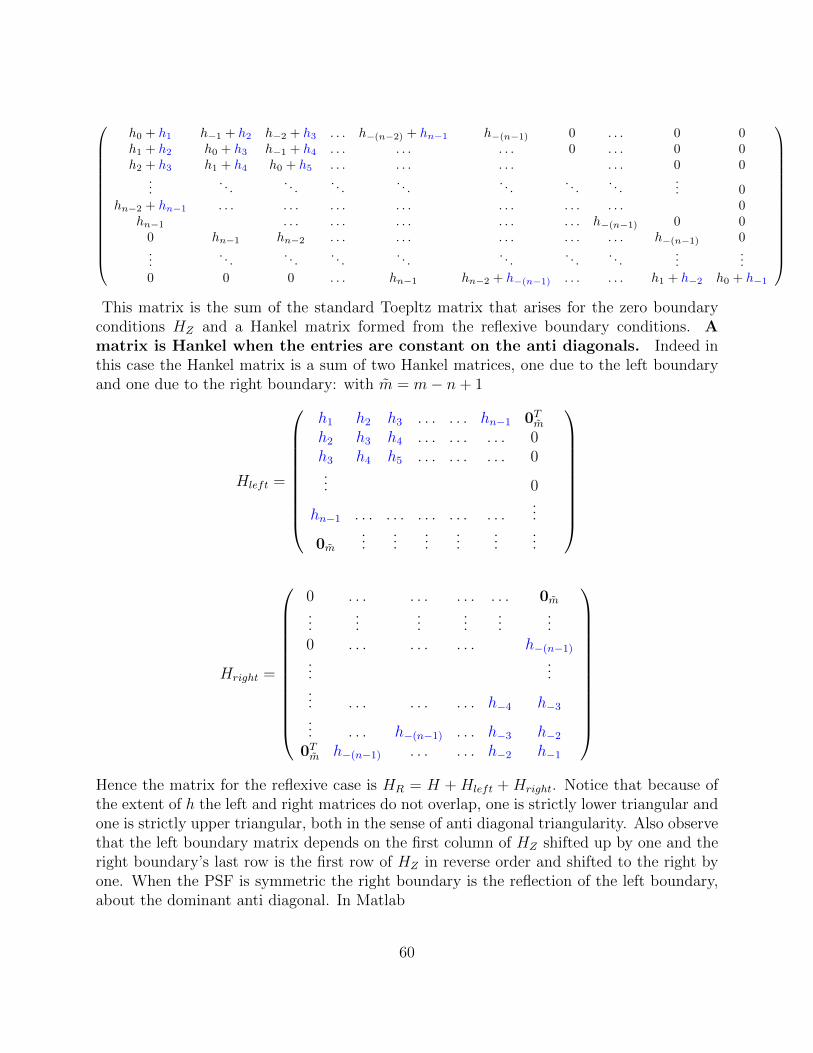
h0 + h1 h−1 + h2 h−2 + h3 . . . h−(n−2) + hn−1 h−(n−1) 0 . . . 0 0h1 + h2 h0 + h3 h−1 + h4 . . . . . . . . . 0 . . . 0 0h2 + h3 h1 + h4 h0 + h5 . . . . . . . . . . . . 0 0

.... . .

. . .. . .

. . .. . .

. . .. . .

... 0hn−2 + hn−1 . . . . . . . . . . . . . . . . . . . . . 0

hn−1 . . . . . . . . . . . . . . . h−(n−1) 0 00 hn−1 hn−2 . . . . . . . . . . . . . . . h−(n−1) 0...

. . .. . .

. . .. . .

. . .. . .

. . ....

...0 0 0 . . . hn−1 hn−2 + h−(n−1) . . . . . . h1 + h−2 h0 + h−1

This matrix is the sum of the standard Toepltz matrix that arises for the zero boundary

conditions HZ and a Hankel matrix formed from the reflexive boundary conditions. Amatrix is Hankel when the entries are constant on the anti diagonals. Indeed inthis case the Hankel matrix is a sum of two Hankel matrices, one due to the left boundaryand one due to the right boundary: with m = m− n+ 1

Hleft =

h1 h2 h3 . . . . . . hn−1 0Tmh2 h3 h4 . . . . . . . . . 0h3 h4 h5 . . . . . . . . . 0... 0

hn−1 . . . . . . . . . . . . . . ....

0m...

......

......

...

Hright =

0 . . . . . . . . . . . . 0m...

......

......

...0 . . . . . . . . . h−(n−1)

......

... . . . . . . . . . h−4 h−3

... . . . h−(n−1) . . . h−3 h−2

0Tm h−(n−1) . . . . . . h−2 h−1

Hence the matrix for the reflexive case is HR = H + Hleft + Hright. Notice that because ofthe extent of h the left and right matrices do not overlap, one is strictly lower triangular andone is strictly upper triangular, both in the sense of anti diagonal triangularity. Also observethat the left boundary matrix depends on the first column of HZ shifted up by one and theright boundary’s last row is the first row of HZ in reverse order and shifted to the right byone. When the PSF is symmetric the right boundary is the reflection of the left boundary,about the dominant anti diagonal. In Matlab

60

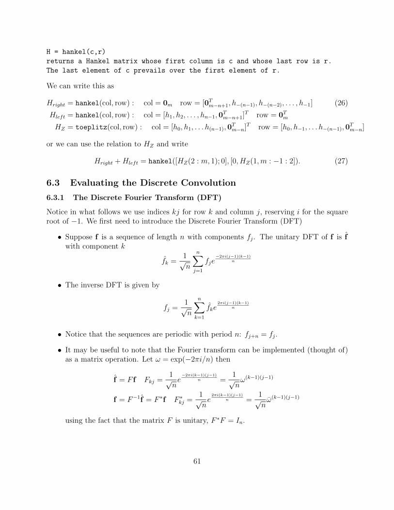
H = hankel(c,r)

returns a Hankel matrix whose first column is c and whose last row is r.

The last element of c prevails over the first element of r.

We can write this as

Hright = hankel(col, row) : col = 0m row = [0Tm−n+1, h−(n−1), h−(n−2), . . . , h−1] (26)

Hleft = hankel(col, row) : col = [h1, h2, . . . , hn−1,0Tm−n+1]T row = 0Tm

HZ = toeplitz(col, row) : col = [h0, h1, . . . h(n−1),0Tm−n]T row = [h0, h−1, . . . h−(n−1),0

Tm−n]

or we can use the relation to HZ and write

Hright +Hleft = hankel([HZ(2 : m, 1); 0], [0, HZ(1,m : −1 : 2]). (27)

6.3 Evaluating the Discrete Convolution

6.3.1 The Discrete Fourier Transform (DFT)

Notice in what follows we use indices kj for row k and column j, reserving i for the squareroot of −1. We first need to introduce the Discrete Fourier Transform (DFT)

• Suppose f is a sequence of length n with components fj. The unitary DFT of f is fwith component k

fk =1√n

n∑j=1

fje−2πi(j−1)(k−1)

n

• The inverse DFT is given by

fj =1√n

n∑k=1

fke2πi(j−1)(k−1)

n

• Notice that the sequences are periodic with period n: fj+n = fj.

• It may be useful to note that the Fourier transform can be implemented (thought of)as a matrix operation. Let ω = exp(−2πi/n) then

f = F f Fkj =1√ne−2πi(k−1)(j−1)

n =1√nω(k−1)(j−1)

f = F−1f = F ∗f F ∗kj =1√ne

2πi(k−1)(j−1)n =

1√nω(k−1)(j−1)

using the fact that the matrix F is unitary, F ∗F = In.

61

6.3.2 Spectral Decompositions

Relating circulant matrices and the DFT (Chapter 5 Vogel)

Definition 8 (Circulant Right Shift Matrix). The matrix R given by

R =

0 0 . . . 0 11 0 0 . . . 00 1 0 0 . . ..... . .

. . .. . .

...0 . . . 0 1 0

or Rkj = δ([j − k + 1]n) δ(j) = 1 only for j = 0.

satisfies the right shift propertry R(h1, h2, h3, . . . , hn)T = (hn, h1, . . . , hn−1)T , and [k]n indi-cates mod n.

By induction it is easy to show that

Rj(h1, h2, h3, . . . , hn)T = (hn−j+1, hn−j+2, . . . , hn−j)T

and

Rj =

0 0 . . . 1 · · · 0 00 0 0 . . . 1 . . . 0.... . .

. . .. . . . . .

. . ....

0 . . . . . . . . . . . . . . . 11 0 . . . . . . . . . . . . 0

0 1. . . . . . . . . . . . . . .

.... . .

. . .. . . . . . . . . . . .

Position of 1 is n− j + 1

Row j.

Theorem 6.1 (Expressing the circulant matrix in terms of shifts). Let

A =

h1 hn . . . h3 h2

h2 h1 . . . h4 h3

.... . .

. . .. . .

...hn−1 . . . h2 h1 hnhn hn−1 . . . h2 h1

Then, noting R0 = I,

(i) A =∑n−1

j=0 hj+1Rj (periodicity hn+p = hp)

(ii) A = F ∗ΛF, Λ =√n diag(h1, h2, . . . , hn) =

√n diag(h)

(iii) (√nhl, F

∗l ) are the eigenvalue - eigenvector pairs of A.

(iv) λj = (√nFA1)j. Thus (FA1)j = hj.

62

(v) A is normal.

Proof.

(i) This is easy to see from the structure of the Toeplitz matrix with each diagonal de-pendent on one entry for h.

(ii) We use ω = exp(−2πi/n) , then√nFkj = ω(k−1)(j−1),

√nF ∗kj = ω(k−1)(j−1) and

(F ∗F )lk =1

n

n∑j=1

ω(j−1)(k−1)ω(l−1)(j−1)

=1

n

n∑j=1

ω(j−1)(k−l) = δ([k − l]n), F ∗F = FF ∗ = In,

which follows from a well-known equality for the sum of exponentials. Let F ∗l be thelth column of F ∗. We know

F ∗l =1√n

[1, ω(l−1), ω2(l−1), . . . , ω(n−1)(l−1)]T

RF ∗l =1√n

[ω(n−1)(l−1), 1, ω(l−1), . . . , ω(n−1)(l−1)]T ,

(RF ∗l ) =1√nωl−1

(1

ωl−1

)[ω(n−1)(l−1), 1, ω(l−1), . . . , ω(n−1)(l−1)]T

=1√nωl−1

(ω(l−1)

)[ω(n−1)(l−1), 1, ω(l−1), . . . , ω(n−1)(l−1)]T

=1√nωl−1[1, ω(l−1), ω2(l−1), . . . , ω(n−1)(l−1)]T = ωl−1F ∗l .

This holds for l = 1 : n. hence that post multiplication by a diagonal matrix scalesthe columns of the matrix gives

RF ∗ = F ∗diag(1, ω, ω2, . . . , ωn−1)

R = F ∗diag(1, ω, ω2, . . . , ωn−1)F = F ∗diag(ωl−1)F.

Immediately we obtain

Rj = F ∗diag(ωl−1)jF = F ∗diag(ω(l−1)j)F,

where diag(ω(l−1)j) is the diagonal matrix with entry ω(l−1)j in column l. Thus using

63

(i)

A =n−1∑j=0

hj+1Rj =

n−1∑j=0

hj+1F∗diag(ω(l−1)j)F

= F ∗diag(n−1∑j=0

hj+1ω(l−1)j)F = F ∗diag(

n∑j=1

hjω(l−1)(j−1))F

=√nF ∗diag(hl)F =

√nF ∗diag(h)F

= F ∗ΛF, Λ =√n diag(h1, h2, . . . , hn).

(iii) This follows immediately now from (ii) by AF ∗l = λlF∗l =√nhlF

∗l .

(iv) Let (A)1 be the first column of A then observe

FA = ΛF F (A)1 = ΛF1

but F1 = (1/√n)(1, 1, . . . , 1)T hence

(FA1)j = λj/√n = hj.

(v) To show A is normal note AA∗ = F ∗ΛFF ∗ΛF = F ∗(Λ)2F = A∗A.

Calculating Ax and A−1b for A circulant March 26 2014

Given the decomposition A = F ∗ΛF , where Λ is determined by h which defines A, calculateAx by observing that Fx = dft(x) = x and F ∗(ΛFx) = idft(ΛFx). Thus

Ax = F ∗ΛFx = F ∗Λx (28)

=√nF ∗(h. ∗ x) =

√nF ∗(y) where y = h. ∗ x (29)

=√ny (30)

Hence to form x convolve with h to give y, then invert to give√ny. Assuming Λ is non

singular, A−1 = F ∗Λ−1F and

A−1b = F ∗Λ−1Fb = F ∗Λ−1b

=1√nF ∗(b./h.) =

1√nF ∗(y) where y = b./h.

=1√n

y

We thus apply this for the case of periodic boundary conditions: HP = circulant(col),

col = [h0, h1, . . . h(n−1),0m, h−(n−1), . . . h−1]T = hext (31)

64

where hext is h extended to length m. Thus the Fourier Transform matrices are of size m,and we form hext to obtain the spectral decomposition: Important : hext is the first columnof A.

Summary for circulant A

Transform PSF hext = Fmhext = dft(hext)

Forward operation Ax : x = dft(x), y = x. ∗ hext. Ax =√m idft(y)

Inverse Operation A−1b : b = dft(b), y = x./hext. A−1b = 1√

midft(y)

6.3.3 General Case

Suppose that there exists a decomposition A = G∗ΛG, for a transform matrix G, and whereΛ = diag(f(A)) for some function of the entries in A. Denote by x = Gx to indicate thetransform of data x. Then we immediately obtain as for the Fourier transform case:

Ax = G∗ΛGx = G∗Λx (32)

= G∗(f(A). ∗ x) = G∗(y) where y = f(A). ∗ x (33)

= y (34)

where G∗ is the inverse transform for transform matrix G, and using G∗G = I.Again, also assuming that f(A) 6= 0 for any component, then with A−1G∗Λ−1G we have

A−1b = G∗Λ−1Gb = G∗Λ−1b

= G∗(b./ ˆf(A).) = G∗(y) where y = b./ ˆf(A).

= y

We now show that there is an equivalent useful decomposition for the case of reflexiveboundary conditions.

6.3.4 The Discrete Cosine Transform

We suppose that h(t) is defined for 0 ≤ t ≤ π with periodicity h(t + π) = h(t), so thath(t+ pπ) = h(t). Let t be discretized on [0, π] by tl = (2l − 1)π/2n, l = 1 : n, dt = π/n andintroduce the basis vectors wj+1, j = 0 : n− 1 with components

(wj+1)l = cj cos(jtl) cj =

√1/n j = 0√2/n otherwise

which discretize the basis functions cos(jt), and the choice for cj assure ‖wj+1‖22 = 1. More-

over the vectors are orthogonal wTj+1wi+1 = 0, i 6= j, forming the columns of an orthogonal

matrix W . The discrete cosine transform of a vector x is defined by

x = dct(x) = W Tx

65

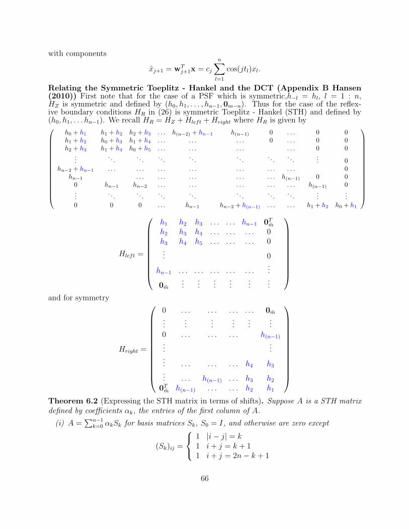
with components

xj+1 = wTj+1x = cj

n∑l=1

cos(jtl)xl.

Relating the Symmetric Toeplitz - Hankel and the DCT (Appendix B Hansen(2010)) First note that for the case of a PSF which is symmetric,h−l = hl, l = 1 : n,HZ is symmetric and defined by (h0, h1, . . . , hn−1,0m−n). Thus for the case of the reflex-ive boundary conditions HR in (26) is symmetric Toeplitz - Hankel (STH) and defined by(h0, h1, . . . hn−1). We recall HR = HZ +Hleft +Hright where HR is given by

h0 + h1 h1 + h2 h2 + h3 . . . h(n−2) + hn−1 h(n−1) 0 . . . 0 0h1 + h2 h0 + h3 h1 + h4 . . . . . . . . . 0 . . . 0 0h2 + h3 h1 + h4 h0 + h5 . . . . . . . . . . . . 0 0

.... . .

. . .. . .

. . .. . .

. . .. . .

... 0hn−2 + hn−1 . . . . . . . . . . . . . . . . . . . . . 0

hn−1 . . . . . . . . . . . . . . . h(n−1) 0 00 hn−1 hn−2 . . . . . . . . . . . . . . . h(n−1) 0...

. . .. . .

. . .. . .

. . .. . .

. . ....

...0 0 0 . . . hn−1 hn−2 + h(n−1) . . . . . . h1 + h2 h0 + h1

Hleft =

h1 h2 h3 . . . . . . hn−1 0Tmh2 h3 h4 . . . . . . . . . 0h3 h4 h5 . . . . . . . . . 0... 0

hn−1 . . . . . . . . . . . . . . ....

0m...

......

......

...

and for symmetry

Hright =

0 . . . . . . . . . . . . 0m...

......

......

...0 . . . . . . . . . h(n−1)

......

... . . . . . . . . . h4 h3

... . . . h(n−1) . . . h3 h2

0Tm h(n−1) . . . . . . h2 h1

Theorem 6.2 (Expressing the STH matrix in terms of shifts). Suppose A is a STH matrixdefined by coefficients αk, the entries of the first column of A.

(i) A =∑n−1

k=0 αkSk for basis matrices Sk, S0 = I, and otherwise are zero except

(Sk)ij =

1 |i− j| = k1 i+ j = k + 11 i+ j = 2n− k + 1

66

i.e. the (i, j) pairs which define the non zero entries of Sk, k ≥ 1, are

(k + j, j), (j − k, j), (k + 1− j, j), (2n− k + 1− j, j)(i, i− k), (i, i+ k), (i, k + 1− i), (i, 2n− k + 1− i)

where here it is assumed that any index less than 1 is invalid. In all cases only twopairs are valid either,

(i, i− k), (i, 2n− k + 1− i) & (i, i+ k), (i, k + 1− i).

(ii) The discrete cosine vectors wj+1 are eigenvectors for each of the basis matrices Sk,with eigenvalue 2 cos(jkπ/n). Hence they are also eigenvectors of A.

(iii) The decomposition A = WΛW t follows where the diagonal matrix is (Λ)j = λj.

(iv)A1 = Ae1 = WΛW Te1 ↔ W TA1 = ΛW Te1.

Consequently, the eigenvalues are λj = dct(A1)]j/[dct(e1)]j

(v) A is normal.

Proof.

(i) For this we note that the matrix is fully defined by the entries in the first column.Thus for a given entry it suffices to find the non zero entries of the particular matrixSk. It is not difficult to find the mutually exclusive pairs in each case showing thatthere are two entries in each column, except for the case with k = 0.

(ii) We form the product Skwj+1. When k = 0 the result follows immediately becauseS0 = I. Otherwise, ignoring the scale factor cj which will cancel,

(Skwj+1)l =n∑p=1

(Sk)lp(wj+1)p = (wj+1)l−k + (wj+1)l+k + (wj+1)k+1−l + (wj+1)2n−k+1−l

= cos(jtl−k) + cos(jtl+k) + cos(jtk+1−l) + cos(jt2n−k+1−l)

= cos(jtl+k) + cos(jtk+1−l)

where the last step occurs by noting only two pairs are valid in each case and by theperiodicity of cos their impact is the same. Now

cos(jtl+k) + cos(jtk+1−l) = cos((2(l + k)− 1)jπ/2n) + cos((2(k − l + 1)− 1)jπ/2n)

= cos((2k + (2l − 1))jπ/2n) + cos((2k − (2l − 1))jπ/2n)

= 2 cos(jkπ/n) cos((2l − 1)jπ/2n) = 2 cos(jkπ/n)(wj+1)l.

Thus wj+1 is an eigenvector of Sk, with eigenvaue 2 cos(jkπ/n) and hence of A for allpairs (k, j)

67

(iii) The decomposition follows immediately by notingAwj+1 = λj+1wj+1 yields wTi+1Awj+1 =

λj+1wTi+1wj+1 = δij and note (W TAW )ij = wT

i+1Awj+1. Hence W TAW = Λ and thedecomposition follows.

(iv) It is immediate that (A)1 = Ae1. But by part (iii) AW = WΛ for matrix W formedfrom the eigenvectors and where Λ is the diagonal matrix of eigenvalues. Thus Ae1 =WΛW Te1 and it follows that W TA1 = ΛW Te1. But W Te1 = dct(e1) and W TA1 =dct(A1). Thus dct(A1) = Λdct(e1) and λj = dct(A1)j/dct(e1)j and the spectrum isdetermined by the first column of the STH matrix A.

(v) A is normal follows as before.

Calculating Ax and A−1b for A STH

Given the decomposition A = WΛW T , where Λ is determined by h which defines A, calculateAx by observing that W Tx = dct(x) = x and W (ΛW Tx) = idct(ΛW Tx). Thus

Ax = WΛW Tx = WΛx, h = dct(A1)./dct(e1)

= W (h. ∗ x) = W (y) where y = h. ∗ x

= y

Hence to form h convolve with x to give y, then invert to give y. Assuming Λ is non singular,A−1 = WΛ−1W T and

A−1b = WΛ−1W Tb = WΛ−1b

= W (b./h.) = W (y) where y = b./h.

= y

For the reflexive case therefore we have A = HZ +Hleft +Hright where for symmetic PSF hwe have

Hright = hankel(col, row) : col = 0m row = [0Tm−n+1, h(n−1), h(n−2), . . . , h1]

Hleft = hankel(col, row) : col = [h1, h2, . . . , hn−1,0Tm−n+1]T row = 0Tm

HZ = toeplitz(col, row) : col = [h0, h1, . . . h(n−1),0Tm−n]T = row = [h0, h1, . . . h(n−1),0

Tm−n]

HZ = toeplitz(row).

We thus apply this for the case of reflexive boundary conditions: HR, formed from HZ

and the left and right boundary condition matrices. Thus the Discrete Cosine Transformmatrices are of size m, and the spectrum again depends on the first column of HR.

Summary for STH A = HR

68

Transform first column which depends on the PSF

h = dct(A1)./dct(e1). (35)

Forward operation Ax : x = dct(x), y = x. ∗ h. Ax = idct(y)

Inverse Operation A−1b : b = dct(b), y = x./h. A−1b = idct(y)

Relating the Toeplitz matrix and the DFT March 31 2014 (Vogel Chapter 5)

To calculate the product Ax when A is Toeplitz, embed in a larger circulant matrix. Againsuppose that we have a Toeplitz matrix which is determined by the padded PSF

hext = [0m, h−(n−1), h−(n−2), . . . , h0, . . . , hn−1,0m], m = m− n.Note that this is a symmetric and periodic extension of the PSF, under the assumption thath|l| tends to 0 with increasing |l|. Let col = [h0, . . . , hn−1,0m], row = [h0, h−1, . . . , h−(n−1),0m]and A = toeplitz(col, row). Let matrix C be of the form

C =

[A BB A

]and B chosen to make C circulant. Then we observe that

C

[x0

]=

[AxBx

]and so the forward operation Ax can be calculated using the circulant matrix C, hence byusing the FFT algorithm described in (28)-(30). It is not too difficult to see how to buildthe matrix B from the matrix A under the condition that C is circulant, each row has to beright shifted from the prior row. We obtain matrix B as the Toeplitz matrix defined by

(h1, h2, . . . hn−1, 0, h−(n−1), h−(n−2), . . . , h−1)

which for the extended PSF becomes

(h1, h2, . . . hn−1,0m−2(n−1), h−(n−1), h−(n−2), . . . , h−1)

B = toeplitz(col, row) row = [0,0m, h(n−1), h(n−2), . . . , h1] col = [0,0m, h−(n−1), . . . , h−1]

The first column of C which defines the fft is given by

col = [h0, . . . , hn−1,0m, 0,0m, h−(n−1), h−(n−2), . . . , h−1]

which for symmetric h (standard) is

col = [h0, . . . , hn−1,0m, 0,0m, h(n−1), h(n−2), . . . , h1],

and the forward matrix product is obtained by the first m entries in Cx.Note that we cannot use the inverse C−1b to obtain T−1b, hence this analysis is useful

for defining forward operations which are used in iterative methods. Observe though thatthe information on the spectrum of the forward operator obtained in this way is still useful.

There is another way to relate the matrix C and T which gives explicit infor-mation about the spectrum, see Hansen 2010

69

6.4 Solutions are obtained with respect to a basis

Note that this discussion is relevant for completing the homework finding the regularizationparameter for DCT and DFT expansions for the matrix A.

Fourier decomposition for Circulant A: Periodic Boundary Conditions

Suppose A ∈ RN×N :

• A = F ∗ΛF, F unitary F ∗F = IN ,

• Λ = diag(hext) for hext defined by (31).

• The solution for Ax = b can be expressed in terms of the basis vectors f∗j which arethe columns of F ∗.

x =

√1

N

N∑j=1

bj

hjf∗j =

√1

N

N∑j=1

γjλj

f∗j γj = bj λj = hj. (36)

Cosine decomposition for STH A: Reflexive Boundary Conditions

Suppose A ∈ RN×N :

• A = WΛW T , W orthogonal W TW = IN ,

• Λ = diag(h) for h defined in (35) which is obtained from the discrete cosine transform.

• The solution for Ax = b can be expressed in terms of the basis vectors wj which are

the columns of W and the discrete cosine transform of b, b = dot(b)

x =N∑j=1

bj

hjwj =

N∑j=1

γjλj

wj γj = bj λj = hj. (37)

6.4.1 Summary: Spectral Decomposition of the Solution

• For all cases we have a decomposition of the solution as a sum of basis vectors, gj,where gj = wj for the DCT case and gj = f∗j for the FFT.

• For the Fourier/Cosine cases the order of the spectral components λj is not defined asit is for the SVD.

• We can examine the solution by examining the spectral components in each case. λjare equivalent to the weights σj of the SVD.

• We note that the DFT and DCT provide feasible approaches for finding the spectrumand evaluating the forward and inverse operations. Ay and A−1y for any vector y

70

• Spectral decomposition suggests truncation to remove the components λj which leadto contamination of the solution.

Remark 2 (Relating the DCT expansion and the SVD Expansion). Let |Λ| = diag(|λj|)and Ω = diag(sign(λj)). Then we may observe

A = WΛW T = WΩ|Λ|W T = UT |Λ|W T

gives an SVD-like expansion for A, in which it is clear that U is orthogonal, but the spectralentries in |Λ| are not necessarily ordered from large to small as in the SVD.

Remark 3 (Relating the FFT expansion and the SVD Expansion). In this case we do nothave the same result as in Remark 2 because the FFT expansion is not real and we cannotsimply use the magnitude of the coefficients in Ω. However we will still have the sameproblem with entries in Λ which have small absolute magnitude contributing to sensitivity inevaluating x.

7 Extension to 2D : In Matrix Notation March 31 2014

7.1 Image Convolution 2D PSF

Let x = vec(X), be the matrix X with entries stacked as a vector. i.e. we take the entriesof X ∈ Rm×n column wise and set N = mn,

vec(X) =

x1

x2

...xn

∈ RN

Then the convolution operatorG = H ∗X

is rewritten asAx = b

where A represents the PSF H, and entries of A depend on how this is implemented.

Condition of the problem can still be investigated naıvely for the linear system. This requiresthe generation of the matrix A for a two dimensional problem.

7.1.1 Descriptive Version of 2D Convolution

1. Regard the PSF as a mask with elements in an array.

2. Rotate the PSF array by 180.

71

3. To compute convolution for a certain pixel we have to line up the central point of therotated mask on that pixel

4. Multiply the corresponding elements within the mask

5. Sum the elements within the mask

6. Take account of boundary conditions as for the 1D Case.

7.1.2 Simple Example

X =

x11 x12 x13

x21 x22 x23

x31 x32 x33

H =

h11 h12 h13

h21 h22 h23

h31 h32 h33

G =

g11 g12 g13

g21 g22 g23

g31 g32 g33

Rotated H, align with x22 and multiply

Hflip =

h33 h32 h31

h23 h22 h21

h13 h12 h11

X. ∗Hflip =

x11h33 x12h32 x13h31

x21h23 x22h22 x23h21

x31h13 x32h12 x33h11

where X.∗H denotes element wise multiplication. We then sum all the entries. In the Vec notationwe have

g22 = vec(Hflip)Tvec(X)

as an inner product. All entries are obtained as inner products.

7.1.3 Calculating all entries for the case of zero boundary conditions

Order the entries by columns .

g11

g21

g31

g12

g22

g32

g13

g23

g33

=

h22 h12 h21 h11

h32 h22 h12 h31 h21 h11

h32 h22 h31 h21

h23 h13 h22 h12 h21 h11

h33 h23 h13 h32 h22 h12 h31 h21 h11

h33 h23 h32 h22 h31 h21

h23 h13 h22 h12

h33 h23 h13 h32 h22 h12

h33 h23 h32 h22

x11

x21

x31

x12

x22

x32

x13

x23

x33

Each block is of Toeplitz form and that as a block matrix the matrix is also Toeplitz.

Matrix is block Toeplitz with Toeplitz Blocks BTTB.

72

7.2 Constructing matrix A: Boundary Conditions, April 1, 2014

PSF is usually of finite extent, but for a finite section of an image, convolution with the PSFuses values outside the specific image. If this is not handled correctly, boundary effects willcontaminate the image, leading to artifacts. This is true whether for the forward or inversemodel.

Options as for the 1D case

Zero Padding: Embed the image in a larger image, with sufficient zeros to handle the

extent of the PSF.

O O O

O X O

O O O

Introduces edges, discontinuities, leads to ringing and artificial black borders.

Matrix is block Toeplitz with Toeplitz Blocks BTTB.

Periodicity: Embed the image periodically in a larger image.

X X X

X X X

X X X

Introduces edges, discontinuities, leads to ringing and artificial black borders. Matrix isblock Circulant with Circulant Blocks BCCB. As an example recall the earlier casewith 3× 3 PSF

h22 h12 h32 h21 h11 h31 h23 h13 h33

h32 h22 h12 h31 h21 h11 h33 h23 h13

h12 h32 h22 h11 h31 h21 h13 h33 h23

h23 h13 h33 h22 h12 h32 h21 h11 h31

h33 h23 h13 h32 h22 h12 h31 h21 h11

h13 h33 h23 h12 h32 h22 h11 h31 h21

h21 h11 h31 h23 h13 h33 h22 h12 h32

h31 h21 h11 h33 h23 h13 h32 h22 h12

h11 h31 h21 h13 h33 h23 h12 h32 h22

=

H2 H1 H3

H3 H2 H1

H1 H3 H2

H1 = circulant(h11, h21, h31) = circulant(h.,1)

H2 = circulant(h12, h22, h32) = circulant(h.,2)

H3 = circulant(h13, h23, h33) = circulant(h.,3)

and the entire PSF can be obtained from the first column of A.

73

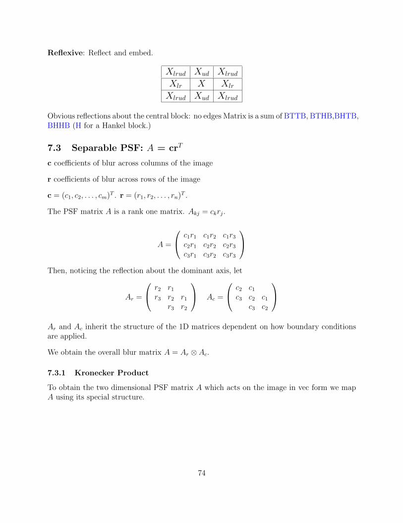
Reflexive: Reflect and embed.

Xlrud Xud Xlrud

Xlr X Xlr

Xlrud Xud Xlrud

Obvious reflections about the central block: no edges Matrix is a sum of BTTB, BTHB,BHTB,BHHB (H for a Hankel block.)

7.3 Separable PSF: A = crT

c coefficients of blur across columns of the image

r coefficients of blur across rows of the image

c = (c1, c2, . . . , cm)T . r = (r1, r2, . . . , rn)T .

The PSF matrix A is a rank one matrix. Akj = ckrj.

A =

c1r1 c1r2 c1r3

c2r1 c2r2 c2r3

c3r1 c3r2 c3r3

Then, noticing the reflection about the dominant axis, let

Ar =

r2 r1

r3 r2 r1

r3 r2

Ac =

c2 c1

c3 c2 c1

c3 c2

Ar and Ac inherit the structure of the 1D matrices dependent on how boundary conditionsare applied.

We obtain the overall blur matrix A = Ar ⊗ Ac.

7.3.1 Kronecker Product

To obtain the two dimensional PSF matrix A which acts on the image in vec form we mapA using its special structure.

74

Ar ⊗ Ac =

a11 a12 · · a1n

a21 a22 · · a2n

· · · · ·· · · · ·am1 am2 · · amn

⊗ Ac

=

a11Ac a12Ac · · a1nAca21Ac a22Ac · · a2nAc· · · · ·· · · · ·

am1Ac am2Ac · · amnAc

7.3.2 Evaluating using the Kronecker Product

Assume Ac ∈ Rm×m and Ar ∈ Rn×n, for an image of size m× n. Note that here we assumethat the matrices Ac and Ar which are defined by PSFs in each dimension, are appropriatelyextended to the appropriate dimension, using reflexive, periodic or zero boundary conditions.Then, for the exact blurred image,

G = AcXATr .

Left multiplication by Ac applies PSF to each column of X, is vertical blur.

Left multiplication of XT by Ar applies PSF to each column of XT , which are rows of X.Hence the horizontal blur is applied as (ArX

T )T = XATr

Let A = Ar ⊗ Ac be the Kronecker product of size mn×mn, the ij block of A is (Ar)ijAc.

Then G = AcXATr in vector form is b = Ax.

Kronecker Product Relations

1.(A⊗B)vec(X) = vec(BXAT )

2. Transpose is distributive(A⊗B)T = (AT ⊗BT )

3. When both matrices are invertible

(A⊗B)−1 = A−1 ⊗B−1

4. Mixed product property for matrices of appropriate dimensions

(A⊗B)(C ⊗D) = (AB ⊗ CD)

5. The Kronecker product is associative, but not commutative.

75

7.4 Spectral Decomposition April 2, 2014

7.4.1 The general case for BCCB

A(h) =

H2 H1 . . . H4 H3

H3 H2 H1 . . . H4

.... . .

. . .. . .

...

Hny

... H3 H2 H1

H1 Hny . . . H3 H2

Each block is circulant, Hj = circulant(h.,j), h of size nx × ny.

A is of size nxny × nxny, n = nxny. The first column defines h.

Again A is normal and we have a spectral decomposition.

A = F ∗diag(√n vec(h))F = F ∗ΛF

Here F = Fr ⊗ Fc and h is the two dimensional FFT of h of size nx × ny. h = F (h) =(Fr ⊗ Fc.)h.

Calculation scheme: A vec(X) = vec(F ∗(λ. ∗ vec(FX))).

As for the 1D case to find eigenvalues of A observe FA = ΛF and F1 = (1/√n)(1, 1, . . . , 1)T ,

(look at the Kronecker product). Hence (√nFA1)l = λl.

For the BCCB first column of A gives h.

Suppose center point of h in spatial domain is at index center = (r0, c0)

Matlab can be used to find this column A1 and F acting on A1 is accomplished as the 2Dtransform

fft2(circshift(h, 1− center)).

i.e. circshift performs necessary circular shift of the PSF matrix.

Note that fft2 in Matlab implements√nF but also ifft2 implements 1/

√nF−1.

7.4.2 DCT analysis extends for the 2D case with reflexive BCs

A = WΛW T

where W is the orthogonal two-dimensional DCT matrix

2D DCT is calculated for array X by computing DCT of each column, followed by DCT ofeach row.

76

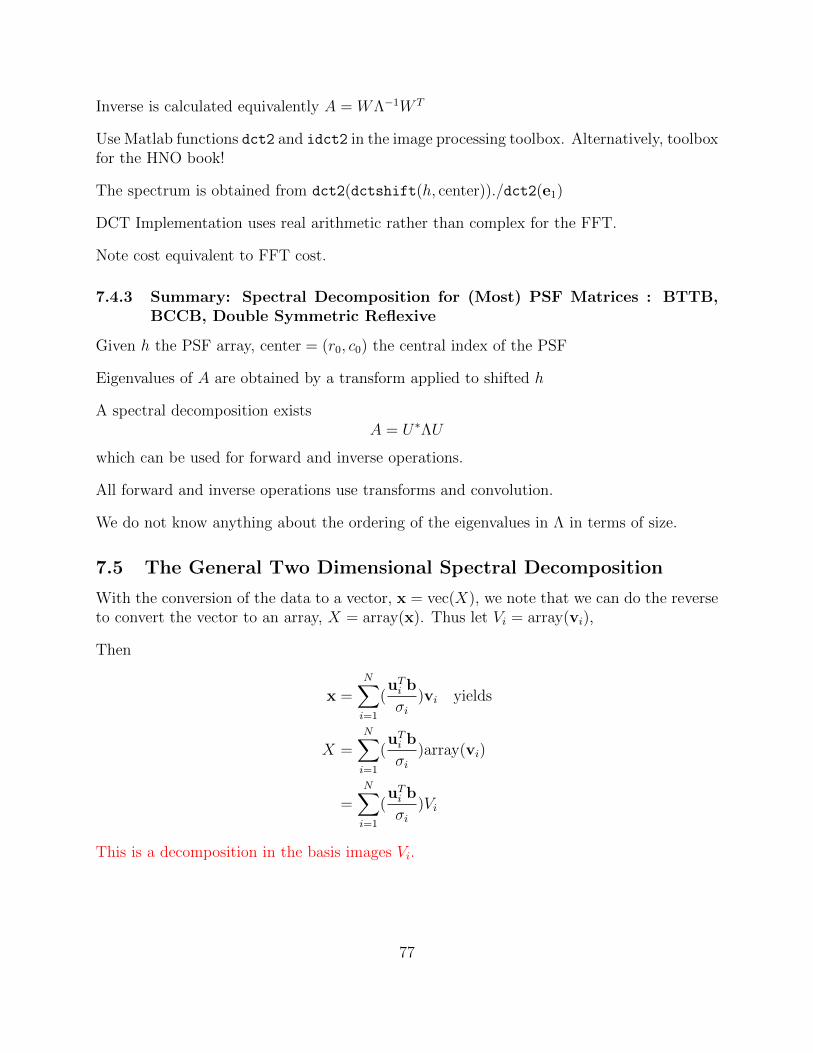
Inverse is calculated equivalently A = WΛ−1W T

Use Matlab functions dct2 and idct2 in the image processing toolbox. Alternatively, toolboxfor the HNO book!

The spectrum is obtained from dct2(dctshift(h, center))./dct2(e1)

DCT Implementation uses real arithmetic rather than complex for the FFT.

Note cost equivalent to FFT cost.

7.4.3 Summary: Spectral Decomposition for (Most) PSF Matrices : BTTB,BCCB, Double Symmetric Reflexive

Given h the PSF array, center = (r0, c0) the central index of the PSF

Eigenvalues of A are obtained by a transform applied to shifted h

A spectral decomposition existsA = U∗ΛU

which can be used for forward and inverse operations.

All forward and inverse operations use transforms and convolution.

We do not know anything about the ordering of the eigenvalues in Λ in terms of size.

7.5 The General Two Dimensional Spectral Decomposition

With the conversion of the data to a vector, x = vec(X), we note that we can do the reverseto convert the vector to an array, X = array(x). Thus let Vi = array(vi),

Then

x =N∑i=1

(uTi b

σi)vi yields

X =N∑i=1

(uTi b

σi)array(vi)

=N∑i=1

(uTi b

σi)Vi

This is a decomposition in the basis images Vi.

77

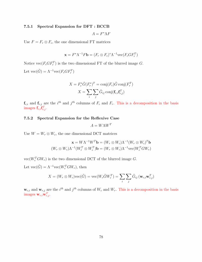
7.5.1 Spectral Expansion for DFT : BCCB

A = F ∗ΛF

Use F = Fr ⊗ Fc, the one dimensional FT matrices

x = F ∗Λ−1Fb = (Fr ⊗ Fc)∗Λ−1vec(FcGFTr )

Notice vec(FcGFTr ) is the two dimensional FT of the blurred image G.

Let vec(G) = Λ−1vec(FcGFTr )

X = F ∗c G(F ∗r )T = conj(Fc)G conj(F Tr )

X =∑i

∑j

Gij conj(fc,ifTr,j)

fc,i and fr,j are the ith and jth columns of Fc and Fr. This is a decomposition in the basisimages fc,if

Tr,j.

7.5.2 Spectral Expansion for the Reflexive Case

A = WΛW T

Use W = Wr ⊗Wc, the one dimensional DCT matrices

x = WΛ−1W Tb = (Wr ⊗Wc)Λ−1(Wr ⊗Wc)

Tb

(Wr ⊗Wc)Λ−1(W T

r ⊗W Tc )b = (Wr ⊗Wc)Λ

−1vec(W Tc GWr)

vec(W Tc GWr) is the two dimensional DCT of the blurred image G.

Let vec(G) = Λ−1vec(W Tc GWr), then

X = (Wr ⊗Wc)vec(G) = vec(WcGWTr ) =

∑i

∑j

Gij (wc,iwTr,j)

wc,i and wr,j are the ith and jth columns of Wc and Wr. This is a decomposition in the basisimages wc,iw

Tr,j.

78

7.5.3 The Separable PSF: A = crT

Matrix A is obtained as Kronecker product A = Ar ⊗ Ac

Ax = AcXATr .

SVD of each matrixAr = UrΣrV

Tr Ac = UcΣcV

Tc

SVD of Kronecker product

(UrΣrVTr )⊗ (UcΣcV

Tc ) = (Ur ⊗ Uc)(Σr ⊗ Σc)(Vr ⊗ Vc)T

Extend the one dimensional SVD solution for b = Ax.

X = VcΣ−1c UT

c GUrΣ−1r V T

r

vec(UcGUTr ) = (Ur ⊗ Uc)Tvec(G) represents the spectral transform of the blurred image G

Let G be the matrix Σ−1c UT

c GUrΣ−1r then

X = VcGVTr = (Vr ⊗ Vc)G =

∑∑Gij(vc,iv

Tr,j)

vc,i and vr,j are the ith and jth columns of Vc and Vr. This is a decomposition in the basisimages vc,iv

Tr,j.

Figure 19: Example taken from Hansen, Nagy and O’Leary, Figure 5.7 Example of basisimages for Middle Size PSF using SVD

79

Figure 20: Example of basis images : Periodic Boundary Conditions Example taken fromHansen, Nagy and O’Leary, Figure 5.8 Notice the periodicity effect on the basis images

Figure 21: Example of basis images : Reflexive Boundary Conditions Example taken fromHansen, Nagy and O’Leary, Figure 5.9 Notice the reflexive effect on the basis images

80

Figure 22: Example of basis images: Periodic BCCB using DFT Example taken from Hansen,Nagy and O’Leary, Figure 5.10 Notice that DFT basis images are quite different.

81

Figure 23: Example of basis images: Doubly Symmetric PSF using DCT Example takenfrom Hansen, Nagy and O’Leary, Figure 5.11 Notice that DCT basis images are again alsoquite different.

7.6 Two Dimensional Problems With Generalized Regularization

Image X : rows in x− direction and columns in y− direction. We know that for regular-ization in the 1D case we introduce a new basis for the solution when using a generalizedregularization. The same should occur in 2D.

Let L be a mapping operator. Mapping in the y direction are achieved by LX, and in thex− direction by (LXT )T = XLT .

If x = vec(X), LX = LX I = (I ⊗ L)x and XLT = IXLT = (L⊗ I)X.

Regularization terms ‖(I ⊗ L)x‖2 and ‖(L⊗ I)x‖2

We note that

‖(I ⊗ L)x‖2 + ‖(L⊗ I)x‖2 =

∣∣∣∣∣∣∣∣( I ⊗ LL⊗ I

)x

∣∣∣∣∣∣∣∣22

is not equivalent to‖((I ⊗ L) + (L⊗ I))x‖2

When L is the first derivative the second expression is the second order Laplacian.

82

7.6.1 Two Dimensions: Assume image is periodic apply Tikhonov Regulariza-tion

When A is the PSF matrix with periodic boundary conditions, and implementable usingDFT matrices F = Fr ⊗ Fc, the regularized Tikhonov solution can be written as

xλ,L = F ∗(|ΛA|2(|ΛA|2 + λ2∆)−1Λ−1A )Fb

∆ is the identity

ΛA is matrix of eigenvalues of A.

|ΛA|2(|ΛA|2 + λ2∆)−1ΛA is diagonal and |ΛA|2(|ΛA|2 + λ2∆)−1 is the filtering matrix.

This corresponds to Wiener filtering.

7.6.2 Two Dimensional Problems using the Fourier Transform

Again suppose A implemented using F = Fr ⊗ Fc, then derivatives are mapped to Fourierdomain

(I ⊗ L) → F ∗(I ⊗ ΛL)F (L⊗ I)→ F ∗(ΛL ⊗ I)F(I ⊗ LL⊗ I

)=

(F ∗ 00 F ∗

)(I ⊗ ΛL

ΛL ⊗ I

)F

and thus regularization terms can all be expressed using the factorization, yielding

xλ,L = F ∗(|ΛA|2|(ΛA|2 + λ2∆)−1Λ−1A )Fb

where now ∆ depends on the regularizer.

83

8 Iterative methods April 14, 2014

8.1 Background

8.1.1 Motivation

For ill-posed problems impossible to construct perfect reconstruction of x

Direct solution methods demonstrate that approximation to x lies in low dimensional sub-space of Rn.

SVD can be used to express solution with respect to a basis

For convolution problems the basis may be a cosine or Fourier basis.

The bases capture the low frequency components of x.

GSVD can be used to express solution with respect to a mapped basis

For large scale problems it is not feasible to find the entire SVD.

Can we find a basis which captures the low frequency information appropriately?

Suppose we are provided with a basis for the solution x, e.g. Kk = spanp1, . . . ,pk whichare columns of a matrix Pk of size n× k. Then we may write the approximation x(k) = Pkyfor some vector y of size k, where we now explicitly assume that the solution x(k) is thekth iterative approximation to x. Therefore finding the solution x(k) which solves the leastsquares problem over the space spanned by Kk can be expressed as the constrained leastsquares problem

x(k) = arg minx‖Ax− b‖2 s.t. x ∈ Kk implies with x = Pky (38)

y(k) = arg miny‖APky − b‖2 (39)

(39) is the projected problem obtained by projecting the original problem to a smaller sub-space.

Given Pk, which is not too large, the solution can be expressed as the solution of the normalequations of size k × k.

Given knowledge of the properties for x, one may be able to find an appropriate basis - e.g.for a symmetric solution the basis should be symmetric.

Moreover, the question becomes how to best pick this basis so that we obtain a good ap-proximation for the solution. Notice that we may write

x(k) =∑i

αiPi = x(k−1) + αkpk, y(k) = (α1, α2, . . . , αk)T

84

Thus, suppose we have x(k−1) to proceed we need to determine how to obtain the next vectorin the underlying space. We want the next vector so that we get a solution which betterminimizes (39), but we know how to solve the normal equations given by (39).

8.2 Conjugate Gradients

We note first the connection between finding the minimum of

φ(x) =1

2xTAx− xTb

and solving Ax = b which follows from solving ∇φ = 0 A is SPD.

Suppose we have solution x(k−1) and wish to find an update

x(k) = x(k−1) + αkpk (40)

which minimizes φ with respect to the scalar αk. In particular, by definition

φ(x(k)) = φ(x(k−1) + αkpk) =1

2(x(k−1) + αkpk)

TA(x(k−1) + αkpk)− (x(k−1) + αkpk)Tb

=1

2

((x(k−1))TAx(k−1) + 2αkp

TkAx(k−1) + α2

kpTkApk

)− (x(k−1) + αkpk)

Tb

=

(1

2(x(k−1))TAx(k−1) − (x(k−1))Tb

)+ αkp

Tk (Ax(k−1) − b) +

1

2α2kp

TkApk

= φ(x(k−1))− αkpTk r(k−1) +1

2α2k‖pk‖2

A, r(k) = b− Ax(k),

where we use the definition pTkApk = ‖pk‖2A, and r(k−1) = Ax(k−1) − b. We now notice that

this depends only on the scalar αk given the direction pk. Minimizing with respect to α, forthe function φ(α) = b/2α2 − aα, the minimum is at φ′(α) = bα − a = 0 or α = a/b, witha = pTk r(k−1) and b = ‖pk‖2

A we obtain

αk =pTk r(k−1)

‖pk‖2A

note by A SPD that‖pk‖2A > 0 (41)

φ(x(k−1) + αkpk) = φ(x(k−1))− 1

2

(pTk r(k−1))2

‖pk‖2A

< φ(x(k−1)), pTk r(k−1) 6= 0. (42)

Hence we know that the basis vector pk should not be orthogonal to the residual vectors,otherwise there is no decrease in the functional. Thus finding a good solution now dependson finding the suitable basis.

Suppose that we have an initial value x(0) then we know that the iterative solutions are givenby

x(k) ∈ x(0) + spanp1, . . . ,pk

85

If the search directions pk are linearly independent and x(k) solves the problem

x(k) = arg minxφ(x) : x ∈ x(0) + spanp1, . . . ,pk

then the iteration has to converge in at most n steps, because the iteration x(n) minimizesφ over Rn and is thus a solution to the system.

The search directions must be easy to compute, i.e. we must be able to compute x(k) easilygiven x(k−1). Let

x(k) = x(0) + Pk−1y + αpk,

then we first note that

r(k−1) = b− Ax(k−1) = b− A(x(0) + Pk−1y) = r(0) − APk−1y

pTk r(k−1) = pTk (r(0) − APk−1y) = pTk r(0) − (pTkAPk−1)y = pTk r(0)

if the pk are A− conjugate. In this case we now see

φ(x(k)) = φ(x(0) + Pk−1y + αpk)

=1

2(x(0) + Pk−1y + αpk)

TA(x(0) + Pk−1y + αpk)− (x(0) + Pk−1y + αpk)Tb

=

(1

2(x(0) + Pk−1y)TA(x(0) + Pk−1y)− (x(0) + Pk−1y)Tb

)+

αpTkA(x(0) + Pk−1y) +1

2α(pk)

TAαpk − α(pk)Tb

= φ(x(0) + Pk−1y)− αpTk r(0) +1

2α2‖pk‖2

A + αpTkAPk−1y.

and the choice of A− conjugacy for pk, namely that pk should be chosen in the spaceorthogonal to spanAp1, . . . , Apk−1 again simplifies this so that

φ(x(k)) = φ(x(0) + Pk−1y)− αpTk r(0) +1

2α2‖pk‖2

A

minx(k)

φ(x(k)) = miny,αφ(x(0) + Pk−1y + αpk)

= minyφ(x(0) + Pk−1y)+ min

α1

2α2‖pk‖2

A − αpTk r(0)

= φ(x(0) + Pk−1y)− 1

2

pTk r(0)

‖pk‖2A

.

and the problem, separates into a pair of uncoupled minimizations.

Suppose that y solves the first problem then x(k−1) minimizes φ over x(0) + span(Pk−1). Thesolution to the second scalar problem is given by (41) but we note

pTk r(k−1) = pTk (b− Ax(k−1)) = pTkb− pTkA(x(0) + Pk−1y) = pTkb− pTkAx(0) = pTk r(0),

86

by the A−conjugacy of the vectors pk. We have an iterative scheme to update x, x(k) =x(k−1) + αkpk as initially desired, provided that we may find

pk ∈ spanAp1, . . . , Ap(k−1)⊥ pTk r(k−1) 6= 0.

For the latter condition, refer to Lemma 10.2.1, Golub and Van Loan, Edition 3.

8.2.1 Choosing the search direction

Suppose that pk is found that minimizes the distance of p to r(k−1) over all vectors thatsatisfy the A-conjugacy:

pk = arg minp∈spanAp1,...,Apk−1

‖p− r(k−1)‖2.

We have to show how to find pk efficiently. First assume that p1 = r(0) and we obtain pkusing the recurrence

pk = r(k−1) − APk−1zk−1, zk−1 = arg minz‖r(k−1) − APk−1z‖2 (43)

We note that this choice yields a small ‖pk‖, by the definition of z(k−1), which is desirableso that x(k) converges, from the update equation (40). We need to show that this choicesatisfies the A−conjugacy and is closest to the latest residual. Since zk−1 solves the leastsquares problem, it satisfies the relevant normal equations

(APk−1)T r(k−1) = (APk−1)T (APk−1)zk−1

0 = (APk−1)T (r(k−1) − APk−1zk−1) = (APk−1)Tpk.

Thus this satisfies the necessary A−conjugacy. Moreover,

pk = r(k−1) − APk−1zk−1 = (I − (APk−1)(APk−1)†)r(k−1) (44)

is by definition the orthogonal projection of r(k−1) into range(APk−1)⊥, which is also thereforethe closest vector in this space to r(k−1). Hence we have the correct choice for pk. With thechoice for the αk this therefore leads to finding the effective stable algorithm. We connectthe approach with the Krylov approach.

8.2.2 Krylov Subspace

Definition 9 (Krylov Subspace). Given an n×n matrix A, a vector b and an integer k theKrylov subspace depending on A, b and k is denoted by

Kk(A,b) = b, Ab, A2b, . . . , Ak−1b (45)

87

We want to connect the solution of the CG iteration with the Krylov subspace dependenton the initial residual r(0). First though, why is this important? We observe the solution ofthe square linear system Ax = b uses the expansion of A−1 using its minimal polynomial(see 6.3 Least Squares Data Fitting with Applications, Hansen et al 2012)

q(t) =k∏j=1

(t− λj)mj

where λj are the distinct eigenvalues of A with multiplicity mj,∑

jmj = n. Then forcoefficients γi

A−1 =n−1∑i=0

γiAi

and the solution may be expressed as

x = A−1b =n−1∑i=0

γiAib ∈ KnA,b.

The dimension of the space is determined by the degree of q(t) and hence by the spectrumof A. If the eigenvalues are clustered with independent eigenvectors then the underlyingspace is smaller. Hence if we use an element of this subspace to provide a solution to thesystem of equations, we will have good convergence if the eigenvalues are clustered ratherthan well-separated.

8.2.3 Connecting CG and Krylov Subspace April 15, 2014

Theorem 8.1 (CG iterations Golub and Van Loan Edition 3, Thm 10.2.3). The followingrelations hold:

1.r(k) = r(k−1) − αkApk (46)

2.P Tk r(k) = 0 (47)

3.spanp1, . . . ,pk = spanr(0)), . . . , r(k−1) = Kk(A, r(0)) (48)

4.(r(j))T r(k) = 0. (49)

Proof. 1. This is easy using the update equation (40) for x(k). Notice that x(k) = x(k−1) +αkpk gives Ax(k) = Ax(k−1) + αkApk and b − Ax(k) = b − Ax(k−1) − αkApk and theresult follows.

88

2. Now use x(k) = x(0) + Pky(k) where y(k) minimizes φ(x(0) + Pky). But

φ(x(0) + Pky) =1

2(x(0) + Pky)TA(x(0) + Pky)− (x(0) + Pky)Tb

= φ(x(0)) + (Pky)T (Ax(0) − b) + (Pky)TAPky

= φ(x(0))− (Pky)T r(0) + (Pky)TAPky.

Given that the first term is fixed, this functional is minimized by minimizing the secondterm −(Pky)T r(0) + (Pky)TAPky. Indeed if this term is zero, then the functional isminimized. But this then means that y solves the system P T

k APky = P Tk r(0). Hence

0 = P Tk (r(0) − APky) = P T

k (b− A(x(0) + Pky)) = P Tk (b− Ax(k)) = P T

k r(k).

3. To connect the subspaces we first note that by (46)

Ap1, . . . , Apk−1 ⊆ r(0), . . . , r(k−1). (50)

Now we have by (44) and by (50)

pk = r(k−1) − APk−1zk−1 ∈ spanr(0), . . . , r(k−1).

Therefore for some upper triangular matrix T we have

Pk = [r(0), . . . , r(k−1)]T

and since the search directions are independent T is nonsingular. Hence

spanp1, . . . ,pk = spanr(0), . . . , r(k−1).

Moreover, by (46)

r(k) ∈ spanr(k−1), Apk ⊆ r(k−1), Ar(0), . . . , Ar(k−1).

We can then apply induction on to obtain the relationship in (48).

4. Finally by (47) r(k) is orthogonal to any vector in range of Pk, which by (48) alsocontains r(0), . . . , r(k−1). The orthogonality of the residuals follows.

This theorem eventually allows us to find that the search directions are obtained by asimple update pk ∈ spanpk−1, r

(k−1), for k ≥ 2.

Theorem 8.2 (Golub and van Loan Edition 3 Corollary 10.2.4). pk ∈ spanpk−1, r(k−1),

for k ≥ 2.

89

Proof. First note p1 = r(0) and p2 ∈ spanr(0), r(1) = spanp1, r(1). For k > 2 we have

pk = r(k−1) − APk−1zk−1 = r(k−1) − APk−2w − µApk−1 by partition of zk−1

= r(k−1) − APk−2w +µ

αk−1

(r(k−1) − r(k−2)) by (46)

=

(1 +

µ

αk−1

)r(k−1) + s(k−1) where s(k−1) = −APk−2w −

µ

αk−1

r(k−2).

Now we obtain

s(k−1) ∈ spanr(k−2), APk−2w⊆ spanr(k−2), Ap1, . . . , Apk−2⊆ spanr(k−2), . . . , r(0).

Now the residuals are mutually orthogonal and so s(k−1) is orthogonal to r(k−1). Hence wenote immediately

‖pk‖2 =

(1 +

µ

αk−1

)2

‖r(k−1)‖2 + ‖s(k−1)‖2

and we can chose µ so that this norm is minimum for the first term. For the second termwe notice that the minimum for ‖s(k−1)‖ = ‖µ/αk−1r

(k−2) + APk−2w‖ is given from (43) byw with

s(k−1) = − µ

αk−1

r(k−2) − APk−2w

= − µ

αk−1

(r(k−2) − APk−2(

−αk−1

µw)

)= − µ

αk−1

(r(k−2) − APk−2zk−2

), w = − µ

αk−1

zk−2

= − µ

αk−1

pk−1,

where the last equality arises from the CG requirement that pk−1 minimizes the given resid-ual. Therefore s(k−1) ∝ pk−1 and we obtain

pk ∈ spanr(k−1),pk−1

8.2.4 Efficient Update Schemes

We now know that we may write pk = r(k−1) + βkpk−1 and want to calculate this efficiently,which requires the calculation of βk. Observe from A−conjugacy

90

0 = pTk−1Apk = pTk−1A(r(k−1) + βkpk−1) yields

βk = −pTk−1Ar(k−1)

pTk−1Apk−1

which requires two matrix-vector multiplications.

Now note that

r(k) = b− Ax(k) = b− A(x(k−1) + αkpk) = r(k−1) − αkApk

(r(k−1))T r(k−1) = −αk−1(r(k−1))TApk−1

0 = (r(k−2))T r(k−2) − αk−1(r(k−2))TApk−1

= (r(k−2))T r(k−2) − αk−1(pk−1 − βk−1pk−2)TApk−1

= (r(k−2))T r(k−2) − αk−1(pk−1)TApk−1

βk =(r(k−1))T r(k−1)

(r(k−2))T r(k−2)

yields the coefficient by two inner products rather than two matrix vector multiplications.

We have in summary the updates

βk =(r(k−1))T r(k−1)

(r(k−2))T r(k−2)=‖r(k−1)‖2

‖r(k−2)‖2(51)

pk = r(k−1) + βkpk−1 (52)

αk =pTk r(k−1)

pTkApk=

pTk r(k−1)

‖pk‖2A

(53)

x(k) = x(k−1) + αkpk (54)

r(k) = r(k−1) − αkApk (55)

which uses only one matrix-vector update per iteration.

Algorithm 1 CG for SPD A with initial guess x(0).

1: k = 0, r(0) = b− Ax(0), p1 = r(0)

2: while r(k) 6= 0 do3: k = k + 14: Update βk by (51)5: Update pk by (52)6: Update αk by (53)7: Update x(k) by (54)8: Update r(k) by (55)9: end while

91

Clearly the algorithm 1 requires improved stopping conditions. This is a topic of particularinterest for ill-posed problems.

Theorem 8.3 (Convergence of CG with respect to the weighted A norm ‖x‖A =√

xTAx).See e.g. Hansen, Pereyra, Scherer Section 6.3 or Golub Theorem 10.2.6, Edition 3.

‖x− x(k)‖A ≤ 1‖x− x(0)‖A(κ(A)− 1

κ(A) + 1

)k8.3 Krylov Methods for the Least Squares Problem April 21 2014

It is immediate from Theorem 8.3 that the convergence of CG depends on the conditionof the matrix, hence applying for the normal equations yields potentially slow convergencedue to the squaring of the condition number. The obvious common variant of Algorithm 1that applies for the normal equations depends on noting that the residual for the normalequations is obtained via

AT (b− Ax) = AT r.

Thus we can modify the updates (51), (52), and (53) as

βk =(AT r(k−1))TAT r(k−1)

(AT r(k−2))TAT r(k−2)(56)

pk = AT r(k−1) + βkpk−1 (57)

αk =‖AT r(k−1)‖2

pTkATApk

(58)

in Algorithm 1 in which the initialization replaces p1 by p1 = AT r(0) giving the algorithmConjugate Gradient Normal Equation Residual (CGNR).

From the derivation of CG it is immediate that CGNR generates the iterate x(k) that mini-mizes

φ1(x) =1

2xT (ATA)x− xT (ATb) over x(0)) +Kk(ATA,AT r(0)). (59)

Since 2φ1(x)+‖b‖2 = ‖Ax−b‖2, x(k) minimizes the least squares cost functional. AlgorithmCGNR is also called CG Least Squares (CGLS) in many places.

It is important to note that the implementation details can drastically impact the stabilityof the algorithm. Observe for example that equations (56), (57) and (58), suggest that itwould be sufficient to directly update qk := AT r(k) and throughout use qk rather than r(k).It has been shown in the literature that this approach is much less stable particularly forlarge condition for A.

For least squares problems a typical starting value is x(0) = 0 so that r(0) = b.

92

8.3.1 Properties of the CGLS iterates

By Theorem 8.1 for x(0) = 0 we know that the underlying subspace for the iteration is theKrylov subspace Kk(ATA,ATb), and therefore although not given explicitly as such we maywrite the solution

x(k) =k−1∑i=0

ci(ATA)iATb

for some constants ci. Use the SVD for A to observe

ATA = (V ΣTUTUΣV T ) = V (ΣTΣ)V T := V Σ2V T , Σ = diag(σ2j ) (60)

(ATA)i = (ATA)(ATA)i−1 = V Σ2V TV Σ2(i−1)V T = V Σ2iV T

(ATA)iAT = (V Σ2iV T )V ΣTUT = V (Σ2iΣT )UT (61)

yielding

x(k) =k−1∑i=0

ciV (Σ2iΣT )UTb

= V

(k−1∑i=0

ciΣ2iΣT

)UTb

=

p∑j=1

φjuTj b

σjvj assuming rank p and φj =

k∑i=1

ci−1σ2ij .

Equivalently x(k) = V ΦkΣ†UTb where Φk is a filter matrix that depends on step k. Clearly

the CGLS solution has a filtered SVD expansion, with filter factors that are polynomial inthe squared singular values σ2

i . Moreover, the contributions due to the small componentsuTj b are less significant in the iteration. Indeed one sees that there is a regularizing effectof the CGLS through the filter matrix Φk so that with each iteration the more dominantfrequencies will be included at the loss of high frequency (small σi) information.

8.4 Methods based on Lanczos Bidiagonalization

Suppose we are given a rectangular matrix A of size m × n and we transform A to lowerbidiagonal form yielding the factorization, with U of size m× n+ 1, V of size n× n and Bn

of size n+ 1× n,

A = U

(Bn

0

)V T , UTU = Im, V TV = InU

TA =

(Bn

0

)V T

(i) : ATU = V(BTn , 0)

(ii) : AV = U

(Bn

0

)(62)

93

Bn =

α1

β2 α2

. . .. . .

βn αnβn+1

To obtain the entries in Bn we equate columns in (62) (i) and (ii)

(i) : ATuj = (V BTn )j = ((BnV

T )row j)T = βjvj−1 + αjvj j = 1 : n β1 = αn+1 = 0

(ii) : Avj = αjuj + βj+1uj+1 j = 1 : n

From which given an initial vector u1 and with αj 6= 0, βj+1 6= 0, we obtain the recursion

vj =ATuj − βjvj−1

αjj = 1 : n

uj+1 =Avj − αjuj

βj+1

j = 1 : n

From here we see this does not completely define the entries. We now impose the orthogo-nality conditions on each of the vectors and replace the updates by

vj = ATuj − βjvj−1, αj = ‖vj‖2, vj = vj/αj j = 1 : n (63)

uj+1 = Avj − αjuj, βj+1 = ‖uj+1‖2, uj+1 = uj+1/βj+1 j = 1 : m (64)

with the assumption that the initial vector is initialized ‖u1‖2 = 1. Clearly the vectorssatisfy

uj ∈ Kj(AAT ,u1) vj ∈ Kj(ATA,ATu1). (65)

8.4.1 LSQR Algorithm (Paige and Saunders - Golub-Kahan bidiagonalization)

Suppose now that we start the algorithm with the initial vector u1 = b/‖b‖2, β1 = ‖b‖2

then we obtain from (65)

uj ∈ Kj(AAT ,b) vj ∈ Kj(ATA,ATb). (66)

Thus for the solution x(k) of the least squares problem we know we want x(k) ∈ Kk(ATA,ATb) =spanv1, . . . ,vk and we can look at the projected solution x(k) = Vky

(k), Vk of size n × k.We obtain, from the definition of u1,

Ax(k) = AVky(k) = Uk+1Bky

(k)

b− Ax(k) = β1u1 − Uk+1Bky(k), Uk+1 of size m× k + 1,

= Uk+1wk+1 wk+1 = β1e1 −Bky(k).

94

Hence to find the optimal solution that minimizes ‖Ax−b‖ over x ∈ Kk(ATA,ATb) we useorthogonality of Uk+1, UT

k+1Uk+1 = Ik+1 to give

min ‖b− Ax(k)‖ = min ‖Uk+1wk+1‖ = min ‖wk+1‖ = min ‖β1e1 −Bky(k)‖

y(k) = β1B†ke1.

The iterative process is the LSQR algorithm of Paige and Saunders, when augmented with afactorization process for the calculation of y(k). For this note that the matrix Bk is bidiagonaland so the solution can be found efficiently using the QR factorization, where the resultingR is upper bidiagonal and efficiently computed with Givens rotations applied to Bk.

We have shown indirectly that to exact precision the following holds.

Theorem 8.4. CGLS and LSQR yield the same sequence of iterates to the solution of theleast squares problem over iterates that are in the space spanned by the columns of Vk.

8.4.2 Projected solution or direct solution April 22, 2014

We have shown that direct methods, e.g. SVD, FFT, obtain the solution in a basis that isdetermined by the matrix A.

Iterative methods yield a solution with a basis determined by the right hand side, startingwith ATb.

It is clear still that noise will enter the solution and hence we must regularize the projectedsolution.

8.4.3 Regularizing the Projected Solution

Regularizing the projected problem we solve

‖Bky(k) − e1 β1‖2 + λ2‖y(k)‖2

Relating to the original full problem we see

‖Ax− b‖2 + λ2‖x‖2 = ‖Bky(k) − e1 β1‖2 + λ2‖V y‖2 = ‖Bky

(k) − e1 β1‖2 + λ2‖y(k)‖2,

which follows by the orthogonality of V . Hence regularizing and projecting is the same asprojecting with regularization, of course when the regularizer is based on ‖x‖.

The regularized problem is of size k+ 1× k. k m and can be solved more efficiently thanthe original problem

Solving the regularized projected problem leads to a hybrid method in which one may onlysolve the regularized version of the problem every certain number of steps k. For a givenregularization parameter choice method, if the regularization parameter converges we assumethat the best solution has been obtained.

95

On the other hand the mechanisms for the regularization choice methods are not immediatelyapplicable.

Nagy uses a weighted GCV - with a fudge factor

the χ2 principle can be extended but the number of degrees of freedom is not clear

Noise revealing properties can be utilized.

Generalized Regularization Consider also the case with regularizer ‖Lx‖, then comparing bothforms with size of Lk chosen consistently as size n× k:

‖Ax(k) − b‖2 + λ2‖Lnx(k)‖2 = ‖w(k)‖2 + λ2‖LnVky(k)‖2

‖Bky(k) − e1 β1‖2 + λ2‖Lky(k)‖2 = ‖w(k)‖2 + λ2‖Lky(k)‖2,

so that solving the normal equations for y(k) in each case

(BTk Bk + λ2(LnVk)

T (LnVk))y(k) = βBT

k e1

(BTk Bk + λ2(LTkLk))y

(k) = βBTk e1

which cannot give the same solution unless we use regularizer Lk = LnVk which makes thesolution of the projected regularized problem expensive, because the typically sparse Ln isreplaced by a dense Lk, while the system matrix Bk is sparse!

Standard Form In order to avoid the problem with the calculation of Lk = LnVk the underlyingfit to data functional for the generalized regularization case is replaced to use a modifiedmatrix A, obtained using the so-called standard form transformation. In this case one needsnot only Ln but also the matrix which spans its null-space, but this is not difficult fortypical choices for matrix Ln, for example Ln may be used to approximate the first orderderivative in which case the constant vector is in the null space. Suppose that H is the matrixformed of the orthonormal basis for the matrix Ln, where Ln approximates the first orderderivative, then H consists of one vector of length n, is constant, with each entry 1/

√n, e.g.

H = 1/√n ones(n, 1). For details of implementing the standard form transformation, see for

example Hansen, 1998.

8.4.4 Propagation of the noise in the Krylov Solution (Not covered)

Clearly the noise enters the solution in a different manner. Suppose n ∼ (0, Cn) where n isthe noise in b. Then ATn ∼ (0, ATCnA), and by (61)

k−1∑i=0

ci(ATA)iATn : =

k−1∑i=0

cini, ni = (ATA)ni−1, i = 1 : k − 1 n0 = ATn (67)

ni ∼ (0, V (Σ2iΣT )UTCnU(ΣΣ2i)V T ), n0 ∼ (0, V ΣTUTCnUΣV T ) (68)

96

as compared to the case for the solution in terms of A, e.g. with the SVD the noise entersvia

(ATA)−1ATn ∼ (0, V (ΣTΣ)−1ΣTUTCnUΣ(ΣTΣ)−1V T )

We have to determine how the variance of∑k−1

i=0 cini is obtained to carefully relate the twoterms. Note that for two random variables X and Y ,

Var(X + Y ) = Var(X) + Var(Y ) + 2Cov(X, Y )

and hence unless X and Y are independent we cannot immediately use linearity. However,we observe from (67) and http://en.wikipedia.org/wiki/Covariance_matrix

Cov(cini, ci−1ni−1) = Cov(ci(ATA)ni−1, ci−1ni−1)

= ci(ATA)ci−1Cov(ni−1,ni−1)

= cici−1(ATA)Cni−1.

Thus

Var(cini + ci−1ni−1) = Var(cini) + Var(ci−1ni−1) + 2Cov(cini, ci−1ni−1)

= c2iCni + c2

i−1Cni−1+ 2cici−1(ATA)Cni−1

= c2i (A

TA)Cni−1(ATA) + c2

i−1Cni−1+ 2cici−1(ATA)Cni−1

(69)

Suppose that Cn = σ2I so that we can move this outside the variance term we obtain forthe direct method

C(ATA)−1ATn = σ2V (ΣTΣ)−1(ΣTΣ)(ΣTΣ)−1V T = σ2V (ΣTΣ)−1V T ,

while for the iterative method

Cn0 = σ2V (ΣTΣ)V T = σ2V (Σ2)V T Σ2 =1

σ2V TCn0V

Cni = σ2V (Σ2iΣT )UTU(ΣΣ2i)V T ) = σ2V (Σ2i(ΣTΣ)Σ2i)V T = σ2V (Σ2(2i+1))V T =

(1

σ2

)2i

C2i+1n0

(ATA)Cni−1=

1

σ2Cn0(

1

σ2)2(i−1)C2(i−1)+1

n0=

(1

σ2

)2i−1

C2in0

and in (69)

Var(cini + ci−1ni−1) =

(1

σ2

)2(i−1)

(ciσ−2Cn0 + ci−1)2C2i−1

n0

= σ2V(c2i Σ

2(2i+1) + c2i−1Σ2(2i−1) + 2cici−1Σ4i

)V T

= σ2V Σ2i(c2i Σ

2 + 2cici−1 + c2i−1Σ−2

)Σ2iV T

= σ2V Σ2i(ciΣ + ci−1Σ−1

)2

Σ2iV T

97

Clearly the mechanism by which noise enters the projected solution is more complicated,and hence it is not immediate that the parameter estimation techniques follow in exactlythe same way as for the full problem. This is a topic for general research.

8.4.5 Extending the UPRE for the LSQR Algorithm

Consider again the UPRE algorithm for the LSQR algorithm. Specifically we form theLanczos procedure to generate bidiagonal matrix B of size (k + 1)× k which satisfies

AV = UB initialized with β = ‖b‖2 for which UTb = βe1, (70)

where V is of size n × k, U of size m × (k + 1), both of which are column orthonormalV TV = Ik, U

TU = Ik+1 and e1 is the unit vector of length k+1. The solution is approximatedby x = V y, where y(Wy) solves the projected problem

y(Wy) = argminy‖By − βe1‖2 + ‖y‖2Wy. (71)

We now examine how to calculate the UPRE from the solution of the projected problem.First observe that from V Tx = V TV y we have yexact = V Txexact. In terms of the projectedproblem the measurable residual is now given by

Ax(Wy)− b = AV y(Wy)− b,

and with

y(Wy) = (BTB +Wy)−1BT (βe1) = (BTB +Wy)−1BT (UTb)

we obtain

Ax(Wy)− b = (AV (BTB +Wy)−1BTUT − Im)b

= (UB(BTUTUB +Wy)−1(UB)T − Im)(bexact + η). (72)

Defining B(Wy) = UB(BTUTUB+Wy)−1(UB)T , we obtain for the LSQR solution, assumingthat A was weighted by the noise in b so that the variance is 1,

E(‖Ax(Wy)− b‖2) = E(‖(B(Wy)− Im)bexact‖2) + trace((B(Wy)− Im)2). (73)

On the other hand, in terms of the projected solution the risk is given by

p(Wy) = A(x(Wy)− xexact)

= B(Wy)(bexact + η)− bexact

= (B(Wy)− I)bexact +B(Wy)η, (74)

for which

E(‖p(Wy)‖2) = E(‖(B(Wy)− I)bexact‖2) + trace(BT (Wy)B(Wy)).

98

Thus following the derivation for the full problem

E(‖p(Wy)‖2) = E(‖Bx(Wy)− b‖2)− trace((B(Wy)− I)2) + trace(BT (Wy)B(Wy))

= E(‖P (Wy)b‖2) + 2trace(B(Wy))−m,

where P (Wy) = Im −B(Wy), which gives the UPRE functional

Uglobal(Wy) = ‖P (Wy)b‖2 + 2trace(B(Wy))−m.

In contrast suppose that we assume that we start with the projected problem (71) and obtainthe UPRE functional directly. For this problem

Uproj = ‖(B(BTB +Wy)−1BT − Ik+1)βe1‖2 + 2trace(B(BTB +Wy)−1BT )− (k + 1)

= ‖UTb‖2 − ‖b‖2 + ‖P (Wy)b‖2 + 2trace(B(BTB +Wy)−1BT )− (k + 1) (75)

where we use UTU = Ik+1. Thus when calculated using the projected problem withoutprojecting to the full problem we calculate

Uproj = Uglobal + 2trace(B(BTB +Wy)−1BT )− 2trace(UB(BTB +Wy)−1BTUT )

+ (m− (k + 1)) + ‖UTb‖2 − ‖b‖2. (76)

Notice, however, by (70) that ‖UTb‖2 = ‖b‖2. We need to compare the eigenvalues ofB(BTB + Wy)−1BT with those of UB(BTB + Wy)−1BTUT , where the second matrix is ofsize m×m and the former of size k+ 1× k+ 1. Now suppose there exists ν and e such that

UB(BTB +Wy)−1BTUTe = νe,

thenB(BTB +Wy)−1BTUTe = νUTe

so that ν is also an eigenvalue of B(BTB + Wy)−1BT , with eigenvector UTe. On the otherhand U is of maximum rank k+ 1, and thus trace(B(BTB+Wy)−1BT ) = trace(UB(BTB+Wy)−1BTUT )2. Thus when seeking to minimize the global predictive risk Uglobal with respectto solving the projected problem, it is sufficient to find the minimum of Uproj. Note that stilldoes not minimize the predictive risk for the full problem.

8.5 Resolution under Regularization by Iteration

The relationship (10) suggests the general form for the resolution matrix. Suppose that x]

is an approximation to the set of equations Ax = b which is obtained as x] = A]b for someapproximation A] for A. The model resolution relationship is thus

x] = A]b = A]Ax = R]x, R] = A]A (77)

2This also follows by the cyclic property of the trace which holds providing that the matrices cycled areconsistent in dimension

99

which defines the approximate resolution matrix R]. For example suppose that A] is obtainedfrom the approximate singular value decomposition of A given by

A ≈ UaΣaVTa

A] = VaΣ−1a UT

a

R] = VaΣ−1a UT

a A,

which can be evaluated. To apply the spike test requires finding the middle column of R],i.e. we need to find,

R]en = R]n, n := bn/2c (78)

R]n ≈ VaΣ

−1a UT

a An. (79)

Alternatively we also note that if we assume the approximate SVD for A then we also have

R] ≈ VaVTa ,

under the assumption on column orthogonality for matrix Ua.For the case of the LSQR algorithm we have, assuming exact arithmetic,

xk = Vkyk, Bkyk ≈ βe1

xk = βVk(BTk Bk)

−1BTk e1 = Vk(B

Tk Bk)

−1BTk U

Tk b

A]k = Vk(BTk Bk)

−1BTk U

Tk = Vk(B

Tk U

Tk UkBk)

−1(UkBk)T

= Vk(BTk U

Tk UkBk)

−1(UkBk)T = Vk((AVk)

T (AVk))−1(AVk)

T

R] = Vk(VTk A

TAVk)−1V T

k (ATA) or

R] = Vk(BTk Bk)

−1BTk U

Tk A = Vk(B

Tk Bk)

−1BTk (ATUk)

T

≈ Vk(BTk Bk)

−1BTk (VkB

Tk + αk+1vk+1e

Tk+1)T = Vk(B

Tk Bk)

−1BTk (BkV

Tk + αk+1ek+1v

Tk+1)

= VkVTk + Vk(B

Tk Bk)

−1(αk+1βk+1ekvTk+1) = VkV

Tk + αk+1βk+1Vk((B

Tk Bk)

−1ek)vTk+1,

and we can find the kth column of (BTk Bk)

−1 approximately. Again if the second term isminimal we may use VkV

Tk to approximate the resolution.

100

9 Extending the Regularization, April 22 2014

A more general regularization term R(x) may be considered to better preserve properties ofthe solution x:

x(λ) = arg minx‖Ax− b‖2

W + λ2R(x) (80)

Suppose R is total variation of x (general options are possible)

The total variation for a function f defined on a discrete grid is

TV(x(a)) =∑i

|x(ai)− x(ai−1)| ≈ ∆∑i

|dx(ai)

da|

TV approximates a scaled sum of the magnitude of jumps in x.

∆ is a scale factor dependent on the grid size.

Two dimensional version

TV(x(a, b)) =∑i,j

√|x(ai, bj)− x(ai−1, bj)|2 + |x(ai, bj)− x(ai, bj−1)|2

≈ ∆∑i,j

√|∂x(ai, bj)/∂a|2 + |∂x(ai, bj)/∂b|2

≈ ∆∑i,j

√|∇x(ai, bj)|2, ∇x = [(∂x(a, b)/∂a)T , (∂x(a, b)/∂b)T ]T

9.1 One Dimensional Case: Using CVX

Notice TV(x(a)) =∑

i |x(ai) − x(ai−1)| = ‖La,1x‖1 where La,1 is the first order derivativematrix operator.

For regularized problem we may want to solve

x(λ) = arg minx‖Ax− b‖2

2 + λ2‖La,1x‖1

Software: Disciplined Convex Programming: an introduction http://cvxr.com/

dcp/ http://cvxr.com/cvx/ describes the general formulation Simple Matlab

m = 20; n = 10; p = 4;

A = randn(m,n); b = randn(m,1);

C = randn(p,n); d = randn(p,1); e = rand;

cvx_begin

variable x(n)

minimize( norm( A * x - b, 2 ) )

subject to

C * x == d

norm( x, Inf ) <= e

cvx_end

101

Using CVX for 1d Problem

x(λ) = arg minx‖Ax− b‖2

2 + λ‖La,1x‖1

In this case use La,1 as the second order derivative smoothing operator. Notice that thisdepends on λ still but no explicit formula is available as for the the Tikhonov case.

cvx_precision(’medium’);

cvx_quiet(false);

cvx_begin

variable x(n);

r = A*x-b;

minimize(lambda*

norm(L*x,1) +r’*r);

cvx_end

Figure 24: A simple example of examining the solution using TV

9.2 Practicalities beyond 1D

For the general problem how can we find the minimum of (80) for R(x) defined by a generalnorm. Consider first that we may write the one dimensional total variation in terms of amatrix operator and an auxiliary function.

Define lTi to be ith row of L1

li = [0, . . . , 0,−1, 1, 0, . . . , 0], x(ai)− x(ai−1) = lTi x

102

where the pair [−1, 1] is in the (i− 1, i)th position. Then

TV (x) =n∑i=2

ψ((lTi x)2), ψ(t) =√t, ψ′(t) =

1

2

1√t

and we see that the derivative is singular at t = 0.

However we know that if we wish to solve a minimization problem we need the gradient ofthe functional (see background in APM 505).

We consider alternative definitions for the functional ψ(t) and introduce approximations forthe total variation of the data.

Suppose that we introduce a perturbation β > 0

ψ(t) =√t+ β2, ψ′(t) =

1

2

1√t+ β2

. (81)

Then the partial derivative ψ′(t) is nonsingular and we approximate the total variationthrough

|x| ≈√|x|2 + β2, 1 β > 0.

Another choice is the Huber function given by

ψ(t) =

t/ε > 0 t ≤ ε2

2√t− ε > 0 t > ε2

(82)

Notice that the choice here for ε makes both ψ and ψ′ continuous.

Moreover the two definitions for ψ are quite close practically.

In particular viable implementation using nonlinear minimization approximates (using thefirst definition for ψ)

TV(x(a, b)) ≈ ∆∑i,j

√|∇x(ai, bj)|2 + β2 =

√‖∇x‖2 + β2

i.e. ∇x ≈ [(La,1x)T , (Lb,1x)T ]T where La,1, Lb,1 denote first order derivatives in a and b.

9.2.1 Review: Newton’s Method April 22, 2014

We minimize the local quadratic approximation in the neighborhood of the minimum of afunction F (x) with respect to a search direction δ:

G(δ) ≈ F (x + δ) ≈ F (x) + (∇F )Tδ +1

2δTHδ,

where H is the Hessian of function F .

103

For this approximation ∇G(δ) = ∇F (x) + Hδ, which is zero when Hδ = −∇F (x). Thisdetermines an alternative search direction to the steepest descent. The convergence rateis typically quadratic, but requires that the initial step is sufficiently close to the solution.A line search is not required as with steepest descent, because the quadratic model shouldprovide an appropriate direction and step length along that direction, but away from thesolution it can be useful to use line search.

Newton’s Method: For given xk solve H(xk)δk = −∇F (xk), and take

xk+1 = xk + αkδk, αk = 1.

Damped Newton’s Method: For given xk solve H(xk)δk = −∇F (xk), and take

xk+1 = xk + αkδk, where αk is chosen to minimize G(αk) = F (xk+1).

Note here this is now a scalar minimization for α.

Secant-Updating- BFGS (Broyden, Fletcher, Goldstein, Shanno)

There are many proposed secant updating formulae for the Hessian, which preserve symmetryand PD, and guarantee that the resulting quasi-Newton step yields a descent step. Indesigning a scheme, it is important to not only preserve symmetry and PD, but also controlerror aspects of the calculation. Mostly the methods are initiated with B0 = I so that theinitial step uses steepest descent. Let yk = ∇F (xk+1)−∇F (xk), then the BFGS update isgiven by

Bk+1 = Bk +yky

Tk

yTk δk− Bkδkδ

TkBk

δTkBkδk≈ Hk+1.

We obtain the algorithm:

Algorithm: BFGS to minimize F (x).Given expression for F (x), and an initial estimate B0(x):

For k = 0, 1, 2, . . .Solve Bkδk = −∇F (xk) for δk !Search Direction

xk+1 = xk + δk !Update solution

yk = ∇F (xk+1)−∇F (xk)

Bk+1 = Bk +yky

Tk

yTk δk− Bkδkδ

TkBk

δTkBkδk!Update approximate Hessian

End

9.2.2 TV Regularization by Newton’s method (Vogel Chapter 8)

For R(x) = TV (x) in a nonlinear minimization we need the gradient (and Hessian) of R(x).

104

Differentiating

∇R(x) = LTdiag(ψ′(x))Lx = Ψ(x)x, Ψ(x) = LTdiag(ψ′(x))L

diag(ψ′(x)) := D1 denotes diagonal matrix with ith entry ψ′((lTi x)2), and the entries arepositive for (81) -(82).

L is SPD provided ψ′(t) > 0 whenever t > 0.

Differentiating again

∇2R(x) = Ψ(x) + Ψ′(x)x, Ψ′(x)x = LTdiag(2(Lx)2ψ′′(x))L = −LTD2L

D2 = −diag(2(Lx)2ψ′′(x)) denotes diagonal matrix with ith entry −2(lTi x)2ψ′′((lTi x)2)

For the functional J(x) = 12‖Ax− b‖2 + λ2R(x) we obtain

∇J(x) = AT (Ax− b) + λ2Ψ(x)x = AT (Ax− b) + λ2LTD1Lx

∇2J(x) = ATA+ λ2Ψ(x) + λ2Ψ′(x)x = ATA+ λ2LTD1L− λ2LTD2L

Notice that once again we need to solve a set of normal equations

(ATA+ λ2Ψ(x) + λ2Ψ′(x)x)δ = −(AT (Ax− b) + λ2Ψ(x)x) (83)

(ATA+ λ2(LT (D1 −D2)L)δ = −[AT (r) + λ2LTD1Lx]. (84)

where r = Ax− b.

For equivalent formulations for 2D see the results in Vogel page 152-153.

9.2.3 Iteratively Reweighted Norm (Rodriguez and Wohlberg 2007 and 2009)

Goal: replace l1 norm by quadratic l2 and iterate to avoid Newton-type approaches

Generally in 2D consider derivative approximations L1,ax = u and L1,bx = v.

R(x) = ||√‖∇x‖2 ||qq =

∑l

(√u2l + v2

l )q =

∑l

(u2l + v2

l )q/2 0 < q ≤ 2

Suppose that W is a diagonal matrix with entries zl = (u2l + v2

l )(q−2)/2, then

‖diag(W 1/2,W 1/2)[uT ,vT ]T‖22 =

∑l

(zl(u2l + v2

l )) =∑l

(u2l + v2

l )q/2. Hence

R(x) = ||(W 1/2 0

0 W 1/2

)(L1,a

L1,b

)x||22 = ‖W 1/2Lx||22,

W = diag(W,W ) L = diag(L1,a, L1,b)

105

Replacing W by W (l) for iteration l, indicating that the elements are calculated usingL1,ax

(k) = u(k) and L1,bx(k) = v(k), z

(k)l = ((u

(k)l )2 + (v

(k)l )2)(q−2)/2 yields

R(k)(x) = ||Lx||2W (k)

To avoid singularity again introduce scaling parameter:

Wll = τ(zl)(zl), τ(z) = 1, z ≥ ε τ(z) = 0, z < ε.

9.2.4 IRN Algorithm

Input: λ, ε, b, A, L, TOL1: Initialize: k = 0, x(k) = (ATA+ λ2LTL)−1ATb2: while ‖x(k) − x(k−1)‖2 > TOL do3: Calculate (Lx(k))T = [u,v]. zl = (u2

l + v2l )

(q−2)/2

4: Update the weighting Wll = τ(u2l + v2

l )(zl)5: Update solution x(k+1) = (ATA+ λ2LTWL)−1ATb (normal equations again)6: k = k + 1,7: end while

• Algorithm was introduced and analysed in Rodriguez and Wohlberg, IEEE Trans SignalProc, 18, 2, 2009, and Signal Processing Letters, 2007.

• Choice of λ using UPRE and trace estimation discussed in Signal Processing, 90, 2010,2546-2551, Lin, Wohlberg and Guo.

• Higher order approach: Yue and Jacob,Biomedical Imaging: From Nano to Macro,2011 IEEE International Symposium, pp.1154-1157, March 30 2011-April 2 2011

9.3 Augmented Lagrangian Approaches : Split Bregman for TV

The main reference is here with software:

T. Goldstein, Split Bregman Software Page, http://www.stanford.edu/~tagoldst/

Tom_Goldstein/Split_Bregman.html.

T. Goldstein and S. Osher, The Split Bregman Method for L1-Regularized Problems.SIAM J. Imaging Sci. 2, 2, (2009), 323-343.

Many developments have been made since that time:

S. Setzer, Operator Splittings, Bregman Methods and Frame Shrinkage in Image Process-ing, International Journal of Computer Vision, in press, 2011.

Above reference discusses relationship of SB to Augmented Lagrangian and Peaceman-Rachford alternating direction

106

9.3.1 SB The Main Idea of GO Paper: for Regularization R(x)

For R(x) = Lx for L ∈ Rq×n: Introduce d = Lx

Rewrite R(x) = λ2‖d− Lx‖2

2 + µ‖d‖1

Anisotropic Formulation:

(x,d) = arg minx,d1

2‖Ax− b‖2

2 +λ

2‖d− Lx‖2

2 + µ‖d‖1

Solve using an alternating minimization which separates minimization for d from x

Derivation uses the Bregman distance and so called Bregman proximal point iteration.

Various versions of the iteration can be defined. Focus on basic formulation here. Iterateover

S1 : x(k+1,l) = arg minx1

2‖Ax− b‖22 +

λ2

2‖Lx− (d(k+1,l−1) − g(k))‖22 (85)

S2 : d(k+1,l) = arg mindλ

2

2‖d− (Lx(k+1,l) + g(k))‖22 + µ‖d‖1 (86)

S3 : g(k+1) = g(k) + Lx(k+1) − d(k+1). (87)

9.3.2 SB Unconstrained algorithm:

Update for x:

x = arg minx1

2‖Ax− b‖2

2 +λ2

2‖Lx− h‖2

2, h = d− g

= arg minx‖Ax− b‖2

2, A =(AT , λLT

)T, b =

(bT , λhT

)T.

Standard least squares update using a Tikhonov regularizer.

Update for d:

d = arg mindµ‖d‖1 +

λ2

2‖d− c‖2

2, c = Lx + g

= arg mind‖d‖1 +

γ

2‖d− c‖2

2, γ =λ2

µ.

This is achieved using soft thresholding.

107

9.3.3 Thresholding for d

If d has q components (d)i componentwise solution:

(d)i =ci|ci|

max(|ci| −1

γ, 0) i = 1 : q

If d is two dimensional it contains components da and db.

L is defined for two dimensions. da = Lax, db = Lbx

Threshold is applied for each component of (dTa ,dTb )T : we use

‖d‖1 = ‖da‖1 + ‖db‖1

The TV norm for the two dimensional case can be written

‖d‖TV = (n∑i=1

‖di‖2) q = 2n

We evaluate for example ∇ = [∇Ta ,∇T

b ]T at each point i in space, there are two componentsat each point.

Intrinsically TV is still local.

(dTV)i =ci‖ci‖2

max(‖ci‖2 −1

γ, 0) i = 1 : n

SB Algorithm

Input: λ, τ , , A, L, σ2

Output: x, d.1: Initialize: k = 0, d(k) = g(k) = x(k) = 0, b(0) = b.2: while ‖Ax− b‖2 > σ2 (DISCREPANCY) do3: while ‖x(k) − x(k−1)‖2 > τ do4: Update x : solve equation (85) where b = b(k)

5: Update d : solve equation (86)6: Update g: equation (87)7: end while8: Update b: equation b(k+1) = b + b(k) − Ad(k+1)

9: end while

In the unconstrained case the outer loop is removed. No update for b are used.The costly step is that for x. Overall cost is basically repeats of quadratic Tikhonov

108

9.3.4 Matlab for SB in One D

function [xk,k]=SB(A, L, b,lambda,mu,tol,itk)

update_x=inline(’(At*A)\At*b’,’A’,’At’,’b’);

update_d=inline(’c./abs(c).*max(abs(c)-1/gamma,0)’,’gamma’,’c’);

gamma=lambda/mu;

[n,p]=size(L);

gk=zeros(n,1); dk=gk; bk=b;hk=gk;xold=bk;testx=xold;

Atilde=[A; sqrt(lambda)*L];k=0;

while ((norm(testx,2)>tol) & (k<itk)),

btilde=[b;sqrt(lambda)*hk];

xk=update_x(Atilde,Atilde’,btilde);

c=L*xk+gk;

dk=update_d(gamma, c);

gk=c-dk;hk=dk-gk;testx=xk-xold;xold=xk;

k=k+1;

end

9.3.5 Solutions with SB

Figure 25: Solution using the Split Bregman algorithm programmed directly

109

9.3.6 Further Discussion on the SB

First we note that the basic step of the SB is a Tikhonov regularization update

S1 : x(k+1) = arg minx1

2‖Ax− b‖2

2 +λ2

2‖Lx− (d(k) − g(k))‖2

2

We can use the GSVD to examine the solution : at the first step (d(k) − g(k)) = 0 and so

xλ =

p∑i=1

νiν2i + λ2µ2

i

(uTi b)zi +n∑

i=p+1

(uTi b)zi

zi is the ith column of (ZT )−1. (A = UΓZT , L = VMZT )

Equivalently with filter factor φi

xλ =

p∑i=1

φiuTi b

νizi +

n∑i=p+1

(uTi b)zi,

Lxλ =

p∑i=1

φiuTi b

ρivi, φi =

ρ2i

ρ2i + λ2

, ρi =νiµi

At subsequent steps the right hand side is changed: Let h(k) = (d(k) − g(k))

Update for x: using the GSVD : basis Z

x(k+1) =

p∑i=1

(νiu

Ti b

ν2i + λ2µ2

i

+λ2µiv

Ti h(k)

ν2i + λ2µ2

i

)zi +

n∑i=p+1

(uTi b)zi

A weighted combination of basis vectors zi: weights

(i)ν2i

ν2i + λ2µ2

i

uTi b

νi(ii)

λ2µ2i

ν2i + λ2µ2

i

vTi h(k)

µi

Notice (i) is fixed by b, but (ii) depends on the updates h(k)

i.e. (i) is iteration independent

If (i) dominates (ii) solution will converge slowly or not at all

110

λ impacts the solution and must not over damp (ii)

x(k+1) =

p∑i=1

(φi

uTi b

νi+ (1− φi)

vTi h(k)

µi

)zi +

n∑i=p+1

(uTi b)zi

Lx(k+1) =

p∑i=1

(φi

uTi b

ρi+ (1− φi)vTi h(k)

)vi.

The stability depends on coefficients

φiρi

1− φiφiνi

1− φiµi

with respect to the inner productsuTi b vTi h(k)

The literature indicates that the choice for λ is problem dependent, and can be picked to beconstant for a given application.

Lets look at what happens as we iterate to see whether it makes sense to keep λ constant.

We can obtain results on determination of optimal choices for the parameter λ. Forexample we can use the UPRE to obtain estimates of the optimal choice for the parameter.

Lemma 3. Suppose noise in h(k) is stochastic and both data fit Ax ≈ b and derivative datafit Lx ≈ h are weighted by their inverse covariance matrices for normally distributed noisein b and h; then optimal choice for λ at all steps is λ = 1.

Remark 4. Can we expect h(k) is stochastic?

Lemma 4. Suppose h(k+1) is regarded as deterministic, then UPRE applied to find the theoptimal choice for λ at each step leads to a different optimum at each step, namely it dependson h.

Remark 5. Because h changes each step the optimal choice for λ using UPRE will changewith each iteration, λ varies over all steps.

111

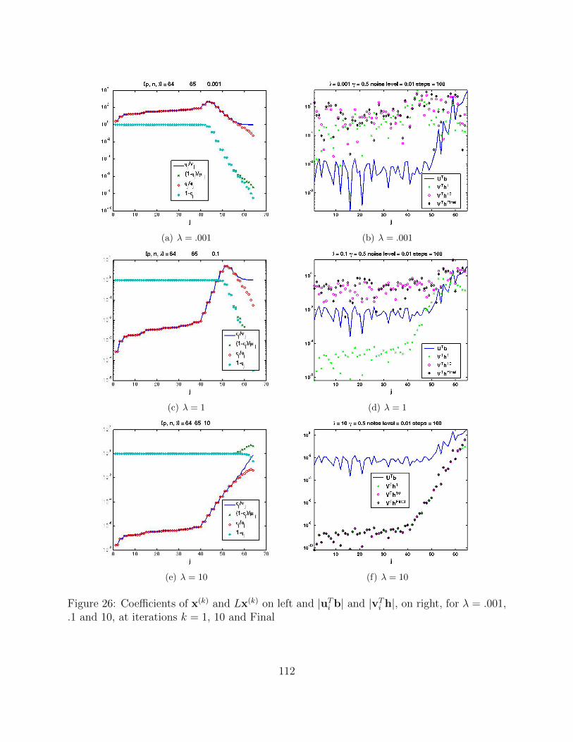
(a) λ = .001 (b) λ = .001

(c) λ = 1 (d) λ = 1

(e) λ = 10 (f) λ = 10

Figure 26: Coefficients of x(k) and Lx(k) on left and |uTi b| and |vTi h|, on right, for λ = .001,.1 and 10, at iterations k = 1, 10 and Final

112

(a) λ = .001 (b) λ = 1 (c) λ = 10

Figure 27: Solutions: λ = .001, .1 and 10

(a) (b)

113

114

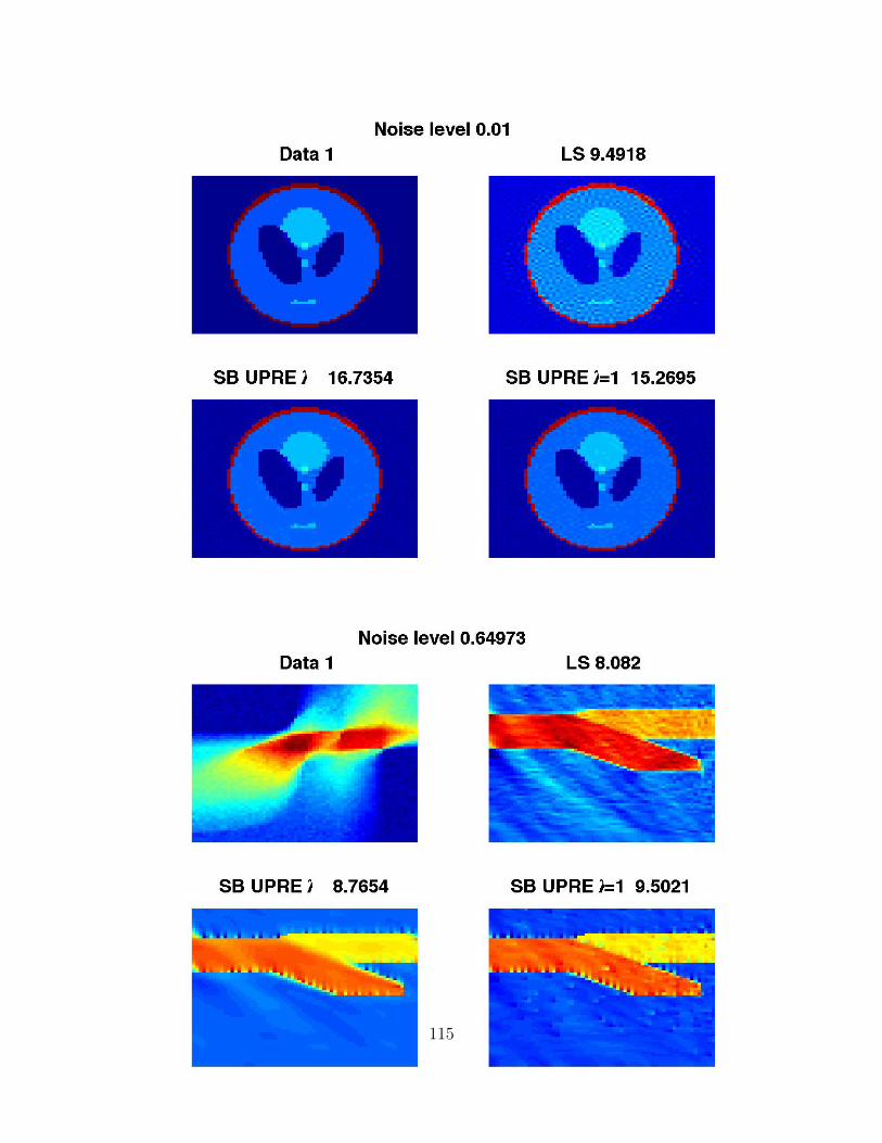
115