Antenna Modeling Considerations - edatop.com

© 2007 ANSYS, Inc. All rights reserved. 1 ANSYS, Inc. Proprietary

Antenna Modeling Considerations

Arien Sligar


Antenna Modeling Guidelines:

What you need to know

• Model setup

– Creating geometry

– Excitations

• Far field considerations

– Radiation boundary vs. PML

– Infinite sphere setup

– Custom integration surface

• Solution setup

– Solution frequency for adaptive meshing

– Choosing a reasonable accuracy

– Output variable convergence

– Direct solver vs. Iterative solver

– Higher order basis functions

– Frequency sweep

• Post processing

– Edit sources

– Output quantities


Model Setup

• Creating Geometry– 2D/3D Metals: Consider tradeoffs

between using 2D vs. 3D metals to modelantennas. Typically using 2D objects torepresent antenna elements will result ina more efficient simulation without animpact on accuracy. 3D metals arenecessary when edge coupling betweenclosely spaced objects is important orwhen the thickness of the object is on theorder of a skin depth.

– Model Detail: Apply engineeringjudgment to determine the level of detailrequired to accurately represent theantenna geometry. Modeling features thatare very small in comparison with awavelength, such as small holes,chamfers, and blends, may unnecessarilyincrease the mesh density in areas thatare not important to the electromagneticbehavior of the antenna.

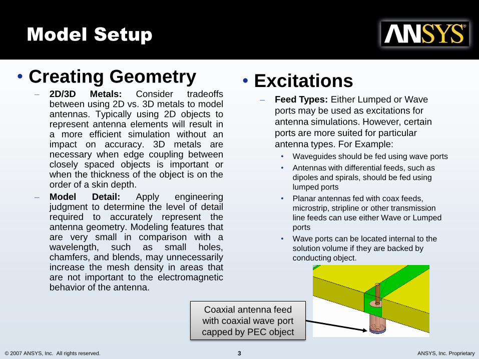
• Excitations– Feed Types: Either Lumped or Wave

ports may be used as excitations for

antenna simulations. However, certain

ports are more suited for particular

antenna types. For Example:

• Waveguides should be fed using wave ports

• Antennas with differential feeds, such as

dipoles and spirals, should be fed using

lumped ports

• Planar antennas fed with coax feeds,

microstrip, stripline or other transmission

line feeds can use either Wave or Lumped

ports

• Wave ports can be located internal to the

solution volume if they are backed by

conducting object.

Coaxial antenna feed

with coaxial wave port

capped by PEC object


Far Field Considerations:

Radiation vs. PML

Solution Volume Size: To properly model the far field behavior of an antenna, an appropriate volume

of air must be included in the simulation. Truncation of the solution space is performed by including

a radiation or PML boundary condition on the faces of this air volume that mimics free space. The

appropriate distance between strongly radiating structures and the nearest face of the air volume

depends upon whether a radiation or PML boundary condition is used.

Radiation Boundary Condition (ABC):

• Absorption achieved via 2nd order radiation boundary

• Place at least λ/4 from strongly radiating structure

• Place at least λ/10 from weakly radiating structure

• The radiation boundary will reflect varying

amounts of energy depending on the incidence

angle. The best performance is achieved at

normal incidence. Avoid angles greater then

~30degrees. In addition, the radiation boundary

must remain convex relative to the wave

Perfectly Matched Layer (PML):

• Fictitious lossy anisotropic material which fully

absorbs electromagnetic fields

• Place at least λ/8 from strongly radiating

structure

• PML thickness should be approximately λ/3 at

the lowest frequency of interest

• Does not suffer from incident angle issues


• The infinite sphere setup specifies a set of spatial data points in a spherical coordinate system for

which HFSS will calculate far-fields. To create an infinite sphere setup:

– Right-click on Radiation Insert Far Field Setup Infinite Sphere

• Relative coordinate systems may be used to modify reference orientation in far-field calculations.

For example the far field coordinate system does not have to be the same as the global coordinate

system.


Infinite Sphere Setup



Custom Integration Surface

• HFSS calculates far fields using a near to far field transformation. The default integration surfaces for the far-field calculations are faces of radiation boundaries. Radiation surfaces are automatically defined on base object faces of PML objects

• Consider creating custom radiation surface for better accuracy and reduced simulation time. This can be done by creating a “virtual object” having the same properties of the surrounding material. Typically the material is air or vacuum for most antennas.

– Place an air box at least /10 from all radiating surfaces

– Create using Modeler List Create Face List

– Also consider adding a mesh seeding operation with /6 seeding to the faces of the “virtual air box” to improve far field accuracy.

– This custom integration surface needs to be specified as a custom radiation surface in the Infinite Sphere setup

Default Integration Surface Custom Integration Surface


Solution Setup (1)

• Solution frequency for adaptive meshing: Thesolution frequency sets the frequency at which theadaptive meshing process is performed.

A higher solution frequency yields a more denseinitial mesh for the adaptive mesher. A higherfrequency mesh is generally valid at lowerfrequencies, however a low frequency mesh isgenerally not valid at higher frequencies.

For resonant or narrow band antennas, the solutionfrequency should be set to the center frequency. Forwideband antennas, the solution frequency cantypically be set to a frequency in the upper half of theoperating band.

• Choosing a reasonable accuracy: Set areasonable maximum ΔS convergence value toavoid unnecessary simulation time and RAM usage.A value of 1%-2% is usually sufficient for antennasimulations. Consider the limitations onmeasurement accuracy when specifying this criterion


Solution Setup (2)

• Expression Cache: In addition to the ΔS convergencecriterion used for the adaptive mesher, expressions may bedefined which further constrains the stopping point of theadaptive mesh algorithm.

This is useful for antenna models for which far-fieldparameters are of primary interest. For these models, outputvariable convergence can be applied on a far-field quantityin order to make sure that the fields have converged as wellas the S-parameters.

• Direct vs iterative matrix solver: The iterative matrix solvercan be used to reduce the RAM necessary to solve themodel. This solver uses an iterative solution method to solvethe matrix of unknowns. If the iterative solver is notsuccessful, the matrix is solved using the default direct multi-frontal solver.

• Higher-order basis functions: Selecting a higher-orderbasis function may reduce the mesh density through the useof higher-order polynomials to represent the field behavior ineach mesh element. The default setting of first-order basisfunctions is applicable to most antenna problems. Formodels that contain large volumes of homogeneous materialsuch as air, the use of second-order basis functions may bemore efficient. Mixed order basis functions introduced inHFSS v12 are ideal for problems that have large spaces andsmall details.


Solution Setup (3):

Frequency Sweep Type

• Discrete frequency sweep: The discrete frequency sweep solves the adapted mesh at eachuser-specified frequency. This is the most accurate method, but the runtime scales linearly with thenumber of frequencies. This sweep type provides fields and S-parameters for each frequencypoint.

• Fast frequency sweep: The fast frequency sweep typically produces valid results over bandwidthof several octaves. Set the adaptive mesh near or at the center of the desired band since the fieldsolution is extrapolated around the solved frequency. This sweep type provides fields and S-parameters for each frequency point.

• Interpolating frequency sweep: The interpolating sweep is applicable to narrowband as well asvery wideband sweeps. This sweep type solves the adapted mesh at the start, stop and midpointof the frequency range and iteratively adds frequency points in order to create a curve-fit for allcomplex S-parameters. This sweep type provides only S-parameters for each frequency point andthe field at the solution frequency.

Sweep Type Speed# of Freq.

Points*

Bandwidth

Limit†Saved Fields Memory

Adaptive

Frequency

Discrete

Slow for many

frequency

points

10’s None All FrequenciesSame as Last

Adaptive

Highest In-

band

Frequency

Fast

• Fast for large

sweeps

• Can be

slower for

small sweeps

<10,000 Octave All FrequenciesMore than

Last Adaptive

Center of

Frequency

Band

Interpolating Fast <10,000 NoneOnly

Last Adaptive

Same as Last

Adaptive

Highest In-

band

Frequency


Post Processing:

Edit Sources

• Edit Sources: Edit sources is a post processing operation that sets complex power scaling factorsfor each port

– Access through menu option HFSS Fields Edit Sources

• The coefficients specified are only used in post-processing operations. The scaling factor usedunder edit sources will not affect passive s-parameter results

– E, H, and J fields on 3D geometry

– Far-field plots (patterns)

– Active S-parameters


• Active S-Parameters: Active S-parameters includes allmutual coupling from other ports to produce an “activeS11” response at a given port. Passive S-parametersassume all other ports are loaded in terminal impedanceand there are no reflections from other terminated ports.Active S-parameters represent port response based oncoupled signals from other ports and includes couplingfrom other ports.

• Total Gain vs. Realized Gain: Total Gain is four pi timesthe ratio of an antenna’s radiation intensity in a givendirection to the total power accepted by the antenna.Realized gain is four pi times the ratio of an antenna’sradiation intensity in a given direction to the total powerincident upon the antenna port(s). Realized Gain includesthe impedance mismatch loss associated with the antennafeed.

• Polarization: The electromagnetic field which is radiatedby an antenna into the far field can be decomposed intovarious orthogonal polarization components. The followingcommonly used definitions are based on the direction ofthe electric field vector as the wave propagates throughspace: Right Hand Circular Polarization (RHCP), LeftHand Circular Polarization (LHCP), Theta-Polarized, Phi-Polarized and X,Y,Z –Polarized. Complete descriptions ofthese quantities are available in the HFSS helpdocumentation.

Post Processing:

Far Field Definitions

Power AcceptedU4

Gain Total

Power IncidentU4

Gain Realized

n

k

kp

mp

mkmp S

a

aActiveS

1

:

:

::


• Radiation trace characteristics can be applied to any 2D radiation plot to quickly obtain

beamwidth for any dB threshold (3 dB, etc.) and sidelobe levels and locations

– Right-click on pattern report to activate menu

Post Processing:

Trace Characteristics

Antenna Modeling Considerations - edatop.com

Documents

Transcript of Antenna Modeling Considerations - edatop.com