Antenna Modeling Considerations

© 2007 ANSYS, Inc. All rights reserved. 1 ANSYS, Inc. Proprietary

Antenna Modeling Considerations

Arien Sligar


Antenna Modeling Guidelines:

What you need to know

• Model setup

– Creating geometry

– Excitations

• Far field considerations

– Radiation boundary vs. PML

– Infinite sphere setup

– Custom integration surface

• Solution setup

– Solution frequency for adaptive meshing

– Choosing a reasonable accuracy

– Output variable convergence

– Direct solver vs. Iterative solver

– Higher order basis functions

– Frequency sweep

• Post processing

– Edit sources

– Output quantities


Model Setup

• Creating Geometry– 2D/3D Metals: Consider tradeoffs

between using 2D vs. 3D metals to modelantennas. Typically using 2D objects torepresent antenna elements will result ina more efficient simulation without animpact on accuracy. 3D metals arenecessary when edge coupling betweenclosely spaced objects is important orwhen the thickness of the object is on theorder of a skin depth.

– Model Detail: Apply engineeringjudgment to determine the level of detailrequired to accurately represent theantenna geometry. Modeling features thatare very small in comparison with awavelength, such as small holes,chamfers, and blends, may unnecessarilyincrease the mesh density in areas thatare not important to the electromagneticbehavior of the antenna.

• Excitations– Feed Types: Either Lumped or Wave

ports may be used as excitations for

antenna simulations. However, certain

ports are more suited for particular

antenna types. For Example:

• Waveguides should be fed using wave ports

• Antennas with differential feeds, such as

dipoles and spirals, should be fed using

lumped ports

• Planar antennas fed with coax feeds,

microstrip, stripline or other transmission

line feeds can use either Wave or Lumped

ports

• Wave ports can be located internal to the

solution volume if they are backed by

conducting object.

Coaxial antenna feed

with coaxial wave port

capped by PEC object


Far Field Considerations:

Radiation vs. PML

Solution Volume Size: To properly model the far field behavior of an antenna, an appropriate volume

of air must be included in the simulation. Truncation of the solution space is performed by including

a radiation or PML boundary condition on the faces of this air volume that mimics free space. The

appropriate distance between strongly radiating structures and the nearest face of the air volume

depends upon whether a radiation or PML boundary condition is used.

Radiation Boundary Condition (ABC):

• Absorption achieved via 2nd order radiation boundary

• Place at least λ/4 from strongly radiating structure

• Place at least λ/10 from weakly radiating structure

• The radiation boundary will reflect varying

amounts of energy depending on the incidence

angle. The best performance is achieved at

normal incidence. Avoid angles greater then

~30degrees. In addition, the radiation boundary

must remain convex relative to the wave

Perfectly Matched Layer (PML):

• Fictitious lossy anisotropic material which fully

absorbs electromagnetic fields

• Place at least λ/8 from strongly radiating

structure

• PML thickness should be approximately λ/3 at

the lowest frequency of interest

• Does not suffer from incident angle issues


• The infinite sphere setup specifies a set of spatial data points in a spherical coordinate system for

which HFSS will calculate far-fields. To create an infinite sphere setup:

– Right-click on Radiation Insert Far Field Setup Infinite Sphere

• Relative coordinate systems may be used to modify reference orientation in far-field calculations.

For example the far field coordinate system does not have to be the same as the global coordinate

system.


Infinite Sphere Setup



Custom Integration Surface

• HFSS calculates far fields using a near to far field transformation. The default integration surfaces for the far-field calculations are faces of radiation boundaries. Radiation surfaces are automatically defined on base object faces of PML objects

• Consider creating custom radiation surface for better accuracy and reduced simulation time. This can be done by creating a “virtual object” having the same properties of the surrounding material. Typically the material is air or vacuum for most antennas.

– Place an air box at least /10 from all radiating surfaces

– Create using Modeler List Create Face List

– Also consider adding a mesh seeding operation with /6 seeding to the faces of the “virtual air box” to improve far field accuracy.

– This custom integration surface needs to be specified as a custom radiation surface in the Infinite Sphere setup

Default Integration Surface Custom Integration Surface


Solution Setup (1)

• Solution frequency for adaptive meshing: Thesolution frequency sets the frequency at which theadaptive meshing process is performed.

A higher solution frequency yields a more denseinitial mesh for the adaptive mesher. A higherfrequency mesh is generally valid at lowerfrequencies, however a low frequency mesh isgenerally not valid at higher frequencies.

For resonant or narrow band antennas, the solutionfrequency should be set to the center frequency. Forwideband antennas, the solution frequency cantypically be set to a frequency in the upper half of theoperating band.

• Choosing a reasonable accuracy: Set areasonable maximum ΔS convergence value toavoid unnecessary simulation time and RAM usage.A value of 1%-2% is usually sufficient for antennasimulations. Consider the limitations onmeasurement accuracy when specifying this criterion


Solution Setup (2)

• Expression Cache: In addition to the ΔS convergencecriterion used for the adaptive mesher, expressions may bedefined which further constrains the stopping point of theadaptive mesh algorithm.

This is useful for antenna models for which far-fieldparameters are of primary interest. For these models, outputvariable convergence can be applied on a far-field quantityin order to make sure that the fields have converged as wellas the S-parameters.

• Direct vs iterative matrix solver: The iterative matrix solvercan be used to reduce the RAM necessary to solve themodel. This solver uses an iterative solution method to solvethe matrix of unknowns. If the iterative solver is notsuccessful, the matrix is solved using the default direct multi-frontal solver.

• Higher-order basis functions: Selecting a higher-orderbasis function may reduce the mesh density through the useof higher-order polynomials to represent the field behavior ineach mesh element. The default setting of first-order basisfunctions is applicable to most antenna problems. Formodels that contain large volumes of homogeneous materialsuch as air, the use of second-order basis functions may bemore efficient. Mixed order basis functions introduced inHFSS v12 are ideal for problems that have large spaces andsmall details.


Solution Setup (3):

Frequency Sweep Type

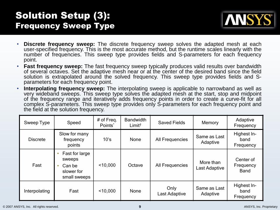
• Discrete frequency sweep: The discrete frequency sweep solves the adapted mesh at eachuser-specified frequency. This is the most accurate method, but the runtime scales linearly with thenumber of frequencies. This sweep type provides fields and S-parameters for each frequencypoint.

• Fast frequency sweep: The fast frequency sweep typically produces valid results over bandwidthof several octaves. Set the adaptive mesh near or at the center of the desired band since the fieldsolution is extrapolated around the solved frequency. This sweep type provides fields and S-parameters for each frequency point.

• Interpolating frequency sweep: The interpolating sweep is applicable to narrowband as well asvery wideband sweeps. This sweep type solves the adapted mesh at the start, stop and midpointof the frequency range and iteratively adds frequency points in order to create a curve-fit for allcomplex S-parameters. This sweep type provides only S-parameters for each frequency point andthe field at the solution frequency.

Sweep Type Speed# of Freq.

Points*

Bandwidth

Limit†Saved Fields Memory

Adaptive

Frequency

Discrete

Slow for many

frequency

points

10’s None All FrequenciesSame as Last

Adaptive

Highest In-

band

Frequency

Fast

• Fast for large

sweeps

• Can be

slower for

small sweeps

<10,000 Octave All FrequenciesMore than

Last Adaptive

Center of

Frequency

Band

Interpolating Fast <10,000 NoneOnly

Last Adaptive

Same as Last

Adaptive

Highest In-

band

Frequency


Post Processing:

Edit Sources

• Edit Sources: Edit sources is a post processing operation that sets complex power scaling factorsfor each port

– Access through menu option HFSS Fields Edit Sources

• The coefficients specified are only used in post-processing operations. The scaling factor usedunder edit sources will not affect passive s-parameter results

– E, H, and J fields on 3D geometry

– Far-field plots (patterns)

– Active S-parameters


• Active S-Parameters: Active S-parameters includes allmutual coupling from other ports to produce an “activeS11” response at a given port. Passive S-parametersassume all other ports are loaded in terminal impedanceand there are no reflections from other terminated ports.Active S-parameters represent port response based oncoupled signals from other ports and includes couplingfrom other ports.

• Total Gain vs. Realized Gain: Total Gain is four pi timesthe ratio of an antenna’s radiation intensity in a givendirection to the total power accepted by the antenna.Realized gain is four pi times the ratio of an antenna’sradiation intensity in a given direction to the total powerincident upon the antenna port(s). Realized Gain includesthe impedance mismatch loss associated with the antennafeed.

• Polarization: The electromagnetic field which is radiatedby an antenna into the far field can be decomposed intovarious orthogonal polarization components. The followingcommonly used definitions are based on the direction ofthe electric field vector as the wave propagates throughspace: Right Hand Circular Polarization (RHCP), LeftHand Circular Polarization (LHCP), Theta-Polarized, Phi-Polarized and X,Y,Z –Polarized. Complete descriptions ofthese quantities are available in the HFSS helpdocumentation.

Post Processing:

Far Field Definitions

Power AcceptedU4

Gain Total

Power IncidentU4

Gain Realized

n

k

kp

mp

mkmp S

a

aActiveS

1

:

:

::


• Radiation trace characteristics can be applied to any 2D radiation plot to quickly obtain

beamwidth for any dB threshold (3 dB, etc.) and sidelobe levels and locations

– Right-click on pattern report to activate menu

Post Processing:

Trace Characteristics

专注于微波、射频、天线设计人才的培养易迪拓培训网址：http://www.edatop.com

射频和天线设计培训课程推荐

易迪拓培训(www.edatop.com)由数名来自于研发第一线的资深工程师发起成立，致力并专注于微

波、射频、天线设计研发人才的培养；我们于 2006 年整合合并微波 EDA 网(www.mweda.com)，现

已发展成为国内最大的微波射频和天线设计人才培养基地，成功推出多套微波射频以及天线设计经典

培训课程和 ADS、HFSS 等专业软件使用培训课程，广受客户好评；并先后与人民邮电出版社、电子

工业出版社合作出版了多本专业图书，帮助数万名工程师提升了专业技术能力。客户遍布中兴通讯、

研通高频、埃威航电、国人通信等多家国内知名公司，以及台湾工业技术研究院、永业科技、全一电

子等多家台湾地区企业。

易迪拓培训课程列表：http://www.edatop.com/peixun/rfe/129.html

射频工程师养成培训课程套装

该套装精选了射频专业基础培训课程、射频仿真设计培训课程和射频电

路测量培训课程三个类别共 30 门视频培训课程和 3 本图书教材；旨在

引领学员全面学习一个射频工程师需要熟悉、理解和掌握的专业知识和

研发设计能力。通过套装的学习，能够让学员完全达到和胜任一个合格

的射频工程师的要求…

课程网址：http://www.edatop.com/peixun/rfe/110.html

ADS 学习培训课程套装

该套装是迄今国内最全面、最权威的 ADS 培训教程，共包含 10 门 ADS

学习培训课程。课程是由具有多年 ADS 使用经验的微波射频与通信系

统设计领域资深专家讲解，并多结合设计实例，由浅入深、详细而又

全面地讲解了 ADS 在微波射频电路设计、通信系统设计和电磁仿真设

计方面的内容。能让您在最短的时间内学会使用 ADS，迅速提升个人技

术能力，把 ADS 真正应用到实际研发工作中去，成为 ADS 设计专家...

课程网址： http://www.edatop.com/peixun/ads/13.html

HFSS 学习培训课程套装

该套课程套装包含了本站全部 HFSS 培训课程，是迄今国内最全面、最

专业的HFSS培训教程套装，可以帮助您从零开始，全面深入学习HFSS

的各项功能和在多个方面的工程应用。购买套装，更可超值赠送 3 个月

免费学习答疑，随时解答您学习过程中遇到的棘手问题，让您的 HFSS

学习更加轻松顺畅…

课程网址：http://www.edatop.com/peixun/hfss/11.html

`

专注于微波、射频、天线设计人才的培养易迪拓培训网址：http://www.edatop.com

CST 学习培训课程套装

该培训套装由易迪拓培训联合微波 EDA 网共同推出，是最全面、系统、

专业的 CST 微波工作室培训课程套装，所有课程都由经验丰富的专家授

课，视频教学，可以帮助您从零开始，全面系统地学习 CST 微波工作的

各项功能及其在微波射频、天线设计等领域的设计应用。且购买该套装，

还可超值赠送 3 个月免费学习答疑…

课程网址：http://www.edatop.com/peixun/cst/24.html

HFSS 天线设计培训课程套装

套装包含 6 门视频课程和 1 本图书，课程从基础讲起，内容由浅入深，

理论介绍和实际操作讲解相结合，全面系统的讲解了 HFSS 天线设计的

全过程。是国内最全面、最专业的 HFSS 天线设计课程，可以帮助您快

速学习掌握如何使用 HFSS 设计天线，让天线设计不再难…

课程网址：http://www.edatop.com/peixun/hfss/122.html

13.56MHz NFC/RFID 线圈天线设计培训课程套装

套装包含 4 门视频培训课程，培训将 13.56MHz 线圈天线设计原理和仿

真设计实践相结合，全面系统地讲解了 13.56MHz线圈天线的工作原理、

设计方法、设计考量以及使用 HFSS 和 CST 仿真分析线圈天线的具体

操作，同时还介绍了 13.56MHz 线圈天线匹配电路的设计和调试。通过

该套课程的学习，可以帮助您快速学习掌握 13.56MHz 线圈天线及其匹

配电路的原理、设计和调试…

详情浏览：http://www.edatop.com/peixun/antenna/116.html

我们的课程优势：

※ 成立于 2004 年，10 多年丰富的行业经验，

※ 一直致力并专注于微波射频和天线设计工程师的培养，更了解该行业对人才的要求

※ 经验丰富的一线资深工程师讲授，结合实际工程案例，直观、实用、易学

联系我们：

※ 易迪拓培训官网：http://www.edatop.com

※ 微波 EDA 网：http://www.mweda.com

※ 官方淘宝店：http://shop36920890.taobao.com

专注于微波、射频、天线设计人才的培养

官方网址：http://www.edatop.com 易迪拓培训淘宝网店：http://shop36920890.taobao.com

Antenna Modeling Considerations

Documents

Transcript of Antenna Modeling Considerations