he electromagnetic spectrum consists of all the frequencies at which electromagnetic waves can occur,

ordered from zero to infinity. Radio waves, visible light, and x rays are examples of electromagnetic waves

at different frequencies. Every part of the electromagnetic spectrum is exploited for some form of scientific

or military activity; the entire spectrum is also key to science and industry. Forensic scientists often use

ultraviolet light technologies to search for latent fingerprints and to examine articles of clothing. Infrared

and near-infrared light technology is used by forensic scientists to record images on specialized film and in

spectroscopy, a tool that determines the chemical structure of a molecule (such as DNA) without

damaging the molecule.

Electromagnetic waves have been known since the mid-nineteenth century, when their behavior was first

described by the equations of Scottish physicist James Clerk Maxwell (1831–1879). Electromagnetic waves,

according to Maxwell's equations, are generated whenever an electrical charge (e.g., an electron) is

accelerated, that is, changes its direction of motion, its speed, or both. An electromagnetic wave is so

named because it consists of an electric and a magnetic field propagating together through space. As the

electric field varies with time, it renews the magnetic field; as the magnetic field varies, it renews the

electric field. The two components of the wave, which always point at right angles both to each other and

to their direction of motion, are thus mutually sustaining, and form a wave which moves forward through

empty space indefinitely.

The rate at which energy is periodically exchanged between the electric and magnetic components of a

given electromagnetic wave is the frequency, ν, of that wave and has units of cycles per second, or Hertz

(Hz); the linear distance between the wave's peaks is termed its wavelength, λ, and has units of length

(e.g., feet or meters). The speed at which a wave travels is the product of its wavelength and its

frequency, V = νλ; in the case of electromagnetic waves, Maxwell's equations require that this velocity

equal the speed of light, c (≅186,000 miles per second [300,000 km/sec]). Since the velocity of all

electromagnetic waves is fixed, the wavelength λ of an electromagnetic wave always determines its

frequency ν, or vice versa, by the relationship c = νλ The higher the frequency (i.e., the shorter the

wavelength) of an electromagnetic wave, the higher in the spectrum it is said to be. Since a wave cannot

have a frequency less than zero, the spectrum is bound by zero at its lower end. In theory, it has no upper

limit.

All atoms and molecules at temperatures above absolute zero radiate electromagnetic waves at specific

frequencies that are determined by the details of their internal structure. In quantum physics, this

radiation must often be described as consisting of particles called photons rather than as waves; however,

this article will restrict itself to the classical (continuous-wave) treatment of electromagnetic radiation,

which is adequate for most technological purposes.

Not only do atoms and molecules radiate electromagnetic waves at certain frequencies, they can absorb

them at the same frequencies. All material objects, therefore, are continuously absorbing and radiating

electromagnetic waves having various frequencies, thus exchanging energy with other objects, near and

far. This makes it possible to observe objects at a distance by detecting the electromagnetic waves that

they radiate or reflect, or to affect them in various ways by beaming electromagnetic waves at them.

These facts make the manipulation of electromagnetic waves at various frequencies (i.e., from various

parts of the electromagnetic spectrum) fundamental to many fields of technology and science, including

radio communication, radar, infrared sensing, visible-light imaging, lasers, x rays, astronomy, and more.

The spectrum has been divided up by physicists into a number of frequency ranges or bands denoted by

convenient names. The points at which these bands begin and end do not correspond to shifts in the

physics of electromagnetic radiation; rather, they reflect the importance of different frequency ranges for

human purposes.

Radio waves are typically produced by time-varying electrical currents in relatively large objects (i.e., at

least centimeters across). This category of electromagnetic waves extends from the lowest-frequency,

longest-wavelength electromagnetic waves up into the gigahertz (GHz; billions of cycles per second)

range. The radio frequency spectrum is divided into more than 450 non-overlapping frequency bands.

These bands are exploited by different users and technologies: for example, broadcast FM is transmitted

using frequencies on the order of 106 Hz, while television signals are transmitted using frequencies on the

order of 108 Hz (about a hundred times higher). In general, higher-frequency signals can always be used to

transmit lower-frequency information, but not the reverse; thus, a voice signal with a maximum frequency

content of 20 kHz (kilohertz, thousands of Hertz) can, if desired, be transmitted on a signal centered in the

Ghz range, but it is impossible to transmit a television signal over a broadcast FM station. Radio waves

termed microwaves are used for high-speed communications links, heating food, radar, and

electromagnetic weapons, that is, devices designed to irritate or injure people or to disable enemy

devices. The microwave frequencies used for communications and radar are subdivided still further into

frequency bands with special designations, such as "X band" and "Y band." Microwave radiation from the

Big Bang, the cosmic explosion in which the Universe originated, pervades all of space.

Electromagnetic waves from approximately 1012 to 5 1014 Hz are termed infrared radiation. The word

infrared means "below red," and is assigned to these waves because their frequencies are just below those

of red light, the lowest-frequency light visible to human beings. Infrared radiation is typically produced by

molecular vibrations and rotations (i.e., heat) and causes or accelerates such motions in the molecules of

objects that absorb it; it is therefore perceived by the body through the increased warmth of skin exposed

to it. Since all objects above absolute zero emit infrared radiation, electronic devices sensitive to infrared

can form images even in the absence of visible light. Because of their ability to "see" at night, imaging

devices that electronically create visible images from infrared light from are important in security systems,

on the battlefield, and in observations of the Earth from space for both scientific and military purposes.

Visible light consists of elecromagnetic waves with frequencies in the 4.3 1014 to 7.5 1014 Hz range. Waves

in this narrow band are typically produced by rearrangements (orbital shifts) in the outer electrons of

atoms. Most of the energy in the sunlight that reaches the Earth's surface consists of electromagnetic

waves in this narrow frequency range; our eyes have therefore evolved to be sensitive to this band of the

electromagnetic spectrum. Photo-voltaic cells—electronic devices that turn incident electromagnetic

radiation into electricity—are also designed to work primarily in this band, and for the same reason.

Because half the Earth is liberally illuminated by visible light at all times, this band of the spectrum, though

narrow (less than an octave), is essential to thousands of applications, including all forms of natural and

many forms of mechanical vision.

Ultraviolet light consists of electromagnetic waves with frequencies in the 7.5 1014 to 1016 Hz range. It is

typically produced by rearrangements in the outer and intermediate electrons of atoms. Ultraviolet light is

invisible, but can cause chemical changes in many substances: for living things, consequences of these

chemical changes can include skin burns, blindness, or cancer. Ultraviolet light can also cause some

substances to give off visible light (flouresce), a property useful for mineral detection, art-forgery

detection, and other applications. Various industrial processes employ ultraviolet light, including

photolithography, in which patterned chemical changes are produced rapidly over an entire film or surface

by projecting patterned ultraviolet light onto it. Most ultraviolet light from the Sun is absorbed by a thin

layer of ozone (O3) in the stratosphere, making the Earth's surface much more hospitable to life than it

would be otherwise; some chemicals produced by human industry (e.g., chlorfluorocarbons) destroy ozone,

threatening this protective layer.

Electromagnetic waves with frequencies from about 1016 to 1019 Hz are termed x rays. X rays are typically

produced by rearrangements of electrons in the innermost orbitals of atoms. When absorbed, x rays are

capable of ejecting electrons entirely from atoms and thus ionizing them (i.e., causing them to have a net

positive electric charge). Ionization is destructive to living tissues because ions may abandon their original

molecular bonds and form new ones, altering the structure of a DNA molecule or some other aspect of cell

chemistry. However, x rays are useful in medical diagnosis and in security systems (e.g., airline luggage

scanners) because they can pass entirely through many solid objects; both traditional contrast images of

internal structure (often termed "x rays" for short) and modern computerized axial tomography images,

which give much more information, depend on the penetrating power of x rays. X rays are produced in

large quantities by nuclear explosions (as are electromagnetic waves at all other frequencies above the

radio band), and have been proposed for use in a space-based ballistic-missile defense system.

All electromagnetic waves above about 1019 Hz are termed gamma rays (g rays), which are typically

produced by rearrangements of particles in atomic nuclei. A nuclear explosion produces large quantities of

gamma radiation, which is both directly and indirectly destructive of life. By interacting with the Earth's

magnetic field, gamma rays from a high-altitude nuclear explosion can cause an intense pulse of radio

waves termed an electromagnetic pulse (EMP). EMP may be powerful enough to burn out unprotected

electronics on the ground over a wide area.

Radio waves present a unique regulatory problem, for only one broadcaster at a particular frequency can

function in a given area. (Signals from overlapping same-frequency broadcasts would be received

simultaneously by antennas, interfering with each other.) Throughout the world, therefore, governments

regulate the radio portion of the electromagnetic spectrum, a process termed spectrum allocation. In the

United States, since the passage of the Communications Act of 1934, the radio spectrum has been deemed

a public resource. Individual private broadcasters are given licenses allowing them to use specific portions

of this resource, that is, specific sub-bands of the radio spectrum. The United States Commerce

Department's National Telecommunications and Information Administration (NTIA) and FCC (Federal

Communications Commission) oversee the spectrum allocation process, which is subject to intense

lobbying by various telecommunications stakeholders.

In summary, it can be said that the manipulation of every level of the electromagnetic spectrum is of

urgent technological interest, but most work is being done in the radio through the visible portions of the

spectrum (below 7.5 1014 Hz), where communications, radar, and imaging can be accomplished.

3. Introduction to Antenna: In the 1890s, there were only a few antennas in the world. These

rudimentary devices were primarily a part of experiments that demonstrated the transmission of

electromagnetic waves. By World War II, antennas had become so ubiquitous that their use had

transformed the lives of the average person via radio and television reception. The number of antennas in

the United States was on the order of one per household, representing growth rivaling the auto industry

during the same period.

    By the early 21st century, thanks in large part to mobile phones, the average person now carries one or

more antennas on them wherever they go (cell phones can have multiple antennas, if GPS is used, for

instance). This significant rate of growth is not likely to slow, as wireless communication systems become

a larger part of everyday life. In addition, the strong growth in RFID devices suggests that the number of

antennas in use may increase to one antenna per object in the world (product, container, pet, banana, toy,

cd, etc.). This number would dwarf the number of antennas in use today. Hence, learning a little (or a large

amount) about of antennas couldn't hurt, and will contribute to one's overall understanding of the modern

world.

Frequency is one of the most important concepts in the universe, which we will see. But fortunately, it isn't

too complicated.

3.1. Antenna: Antennas function by transmitting or receiving electromagnetic (EM) waves. Examples

of these electromagnetic waves include the light from the sun and the waves received by your cell phone

or radio. Your eyes are basically "receiving antennas" that pick up electromagnetic waves that are of a

particular frequency. The colors that you see (red, green, and blue) are each waves of different

frequencies that your eyes can detect.

All electromagnetic waves propagate at the same speed in air or in space. This speed (the speed of

light) is roughly 671 million miles per hour (1 billion kilometers per hour). This is roughly a million times

faster than the speed of sound (which is about 761 miles per hour at sea level). The speed of light will be

denoted as c in the equations that follow. We like to use "SI" units in science (length measured in meters,

time in seconds, and mass in kilograms), so we will forever remember that:

Before defining frequency, we must define what an "electromagnetic wave" is. This is an electric field that

travels away from some source (an antenna, the sun, and a radio tower, whatever). A traveling electric

field has an associated magnetic field with it, and the two make up an electromagnetic wave.

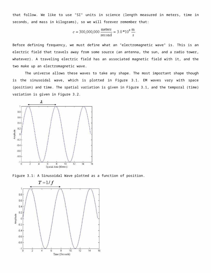
The universe allows these waves to take any shape. The most important shape though is the

sinusoidal wave, which is plotted in Figure 3.1. EM waves vary with space (position) and time. The spatial

variation is given in Figure 3.1, and the temporal (time) variation is given in Figure 3.2.

Figure 3.1: A Sinusoidal Wave plotted as a function of position.

Figure 3.2: A Sinusoidal Wave plotted as a function of time.

The wave is periodic; it repeats itself every T seconds. Plotted as a function in space, it repeats itself every

meter, which we will call the wavelength. The frequency (written f) is simply the number of complete

cycles the wave completes (viewed as a function of time) in one second (two hundred cycles per second is

written 200 Hz, or 200 "Hertz"). Mathematically this is written as:

How fast someone walks depends on the size of the steps they take (the wavelength) multiple by the rate

at which they take steps (the frequency). The speed that the waves travel is how fast the waves are

oscillating in time (f) multiplied by the size of the step the waves are taken per period ( ). The equation

that relates frequency, wavelength and the speed of light can be tattooed on your forehead:

Basically, the frequency is just a measure of how fast the wave is oscillating. And since all EM

waves travel at the same speed, the faster it oscillates the shorter the wavelength. And a longer

wavelength implies a slower frequency.

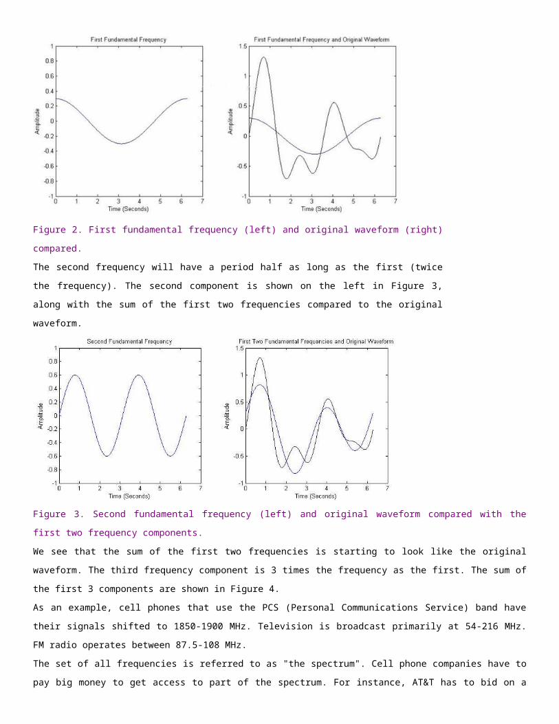
Figure 1. A simple waveform.

As an example, lets break down the waveform in Figure 1 into its 'building blocks' or the

it's frequencies. This decomposition can be done with a Fourier transform (or Fourier

series for periodic waveforms). The first component is a sinusoidal wave with period

T=6.28 (2*pi) and amplitude 0.3, as shown in Figure 2.

Figure 2. First fundamental frequency (left) and original waveform (right) compared.

The second frequency will have a period half as long as the first (twice the frequency).

The second component is shown on the left in Figure 3, along with the sum of the first

two frequencies compared to the original waveform.

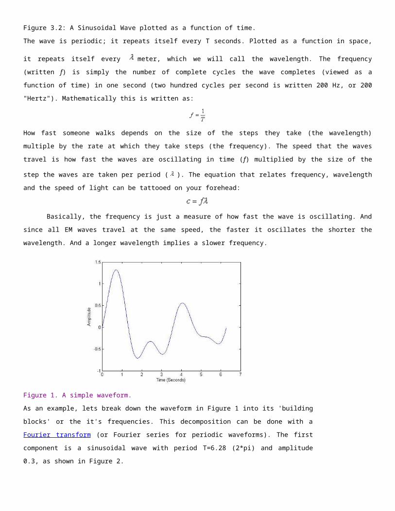
Figure 3. Second fundamental frequency (left) and original waveform compared with the first two

frequency components.

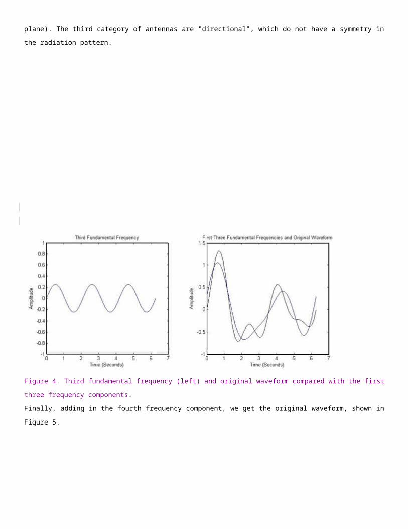
We see that the sum of the first two frequencies is starting to look like the original waveform. The third

frequency component is 3 times the frequency as the first. The sum of the first 3 components are shown in

Figure 4.

As an example, cell phones that use the PCS (Personal Communications Service) band have their signals

shifted to 1850-1900 MHz. Television is broadcast primarily at 54-216 MHz. FM radio operates between

87.5-108 MHz.

The set of all frequencies is referred to as "the spectrum". Cell phone companies have to pay big money to

get access to part of the spectrum. For instance, AT&T has to bid on a slice of the spectrum with the FCC,

for the "right" to transmit information within that band. The transmission of EM energy is greatly regulated.

When AT&T is sold a slice of the spectrum, they can not transmit energy at any other band (technically,

the amount transmitted must be below some threshold in adjacent bands).

The Bandwidth of a signal is the difference between the signals high and low frequencies. For instance, a

signal transmitting between 40 and 50 MHz has a bandwidth of 10 MHz.

We'll wrap up with a table of frequency bands along with the corresponding wavelengths. From the table,

we see that VHF is in the range 30-300 MHz (30 Million-300 Million cycles per second). At the very least

then, if someone says they need a "VHF antenna", you should now understand that the antenna should

transmit or receive electromagnetic waves that have a frequency of 30-300 MHz.

Frequency Band Name Frequency Range Wavelength

(Meters)Application

Extremely Low

Frequency (ELF)3-30 Hz 10,000-100,000 km Underwater Communication

Super Low Frequency

(SLF)30-300 Hz 1,000-10,000 km

AC Power (though not a

transmitted wave)

Ultra Low Frequency

(ULF)300-3000 Hz 100-1,000 km

Very Low Frequency

(VLF)3-30 kHz 10-100 km Navigational Beacons

Low Frequency (LF) 30-300 kHz 1-10 km AM Radio

Medium Frequency (MF) 300-3000 kHz 100-1,000 m Aviation and AM Radio

High Frequency (HF) 3-30 MHz 10-100 m Shortwave Radio

Very High Frequency

(VHF)30-300 MHz 1-10 m FM Radio

Ultra High Frequency

(UHF)300-3000 MHz 10-100 cm Television, Mobile Phones, GPS

Super High Frequency

(SHF)3-30 GHz 1-10 cm

Satellite Links, Wireless

Communication

Extremely High

Frequency (EHF)30-300 GHz 1-10 mm Astronomy, Remote Sensing

Visible Spectrum400-790 THz (4*10^14-

7.9*10^14)

380-750 nm

(nanometers)Human Eye

Table 1. Frequency Bands

Basically the frequency bands each range over from the lowest frequency to 10 times the lowest

frequency. Antenna engineers further divide the bands into things like "X-band" and "Ku-band". That is the

basics of frequency.

Radiation Pattern: A radiation pattern defines the variation of the power radiated by an antenna as a

function of the direction away from the antenna. This power variation as a function of the arrival angle is

observed in the far field.

As an example, consider the 3-dimensional radiation pattern in Figure 1, plotted in decibels (dB) .

In this case, along the z-axis, which would correspond to the radiation directly overhead the antenna, there

is very little power transmitted. In the x-y plane (perpendicular to the z-axis), the radiation is maximum.

These plots are useful for visualizing which directions the antenna radiates.

Typically, because it is simpler, the radiation patterns are plotted in 2-d. In this case, the patterns are

given as "slices" through the 3d plane. The same pattern in Figure 1 is plotted in Figure 2. Standard

spherical coordinates are used, where is the angle measured off the z-axis, and is the angle

measured counterclockwise off the x-axis.

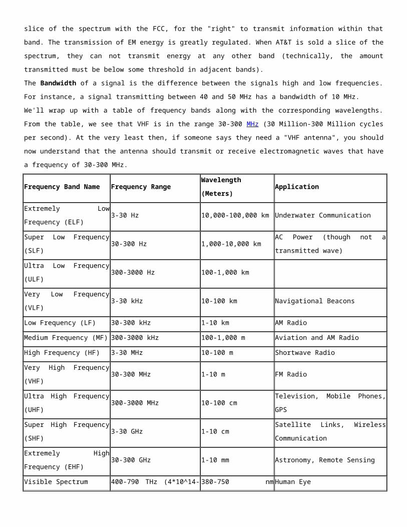
Figure 2. Two-dimensional radiation plots.

A pattern is "isotropic" if the radiation pattern is the same in all directions. These antennas don't exist in

practice, but are sometimes discussed as a means of comparison with real antennas. Some antennas may

also be described as "omnidirectional", which for an actual means that it is isotropic in a single plane (as in

Figure 1 above for the x-y plane). The third category of antennas are "directional", which do not have a

symmetry in the radiation pattern.

   

Figure 4. Third fundamental frequency (left) and original waveform compared with the first three

frequency components.

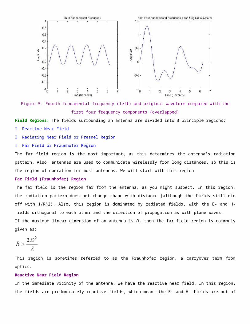
Finally, adding in the fourth frequency component, we get the original waveform, shown in Figure 5.

Figure 5. Fourth fundamental frequency (left) and original waveform compared with the first four

frequency components (overlapped)

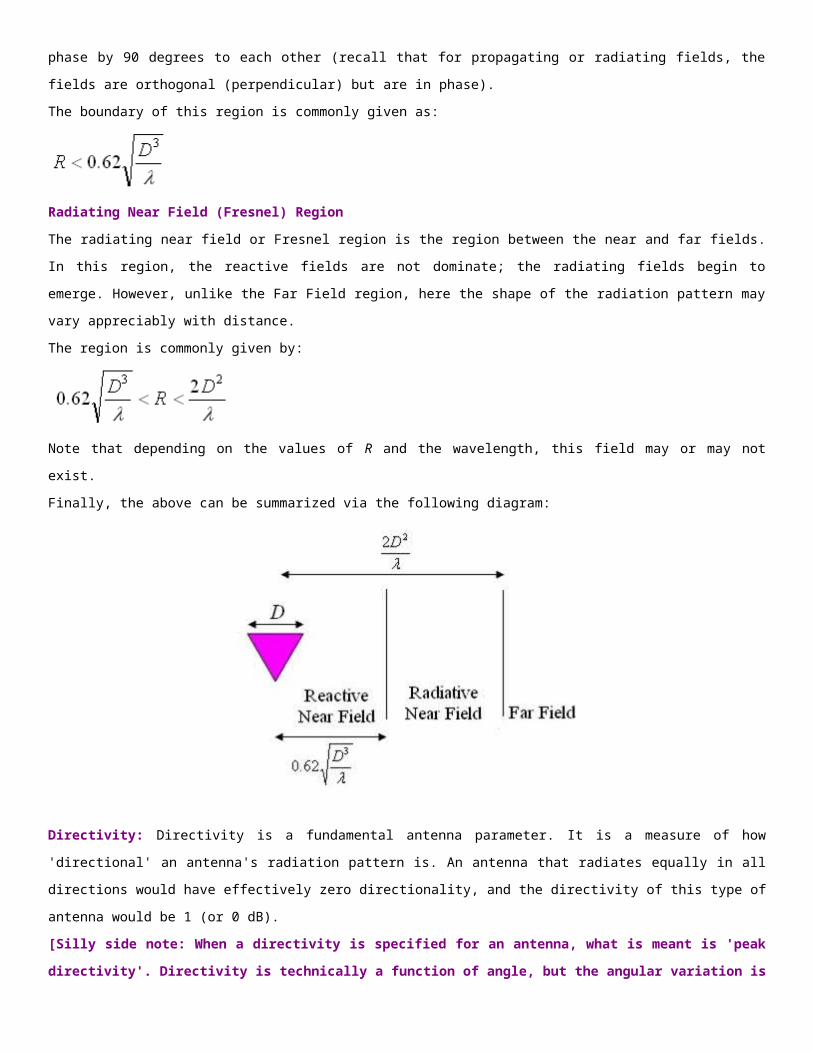
Field Regions: The fields surrounding an antenna are divided into 3 principle regions:

Reactive Near Field

Radiating Near Field or Fresnel Region

Far Field or Fraunhofer Region

The far field region is the most important, as this determines the antenna's radiation pattern. Also,

antennas are used to communicate wirelessly from long distances, so this is the region of operation for

most antennas. We will start with this region

Far Field (Fraunhofer) Region

The far field is the region far from the antenna, as you might suspect. In this region, the radiation pattern

does not change shape with distance (although the fields still die off with 1/R^2). Also, this region is

dominated by radiated fields, with the E- and H-fields orthogonal to each other and the direction of

propagation as with plane waves.

If the maximum linear dimension of an antenna is D, then the far field region is commonly given as:

This region is sometimes referred to as the Fraunhofer region, a carryover term from optics.

Reactive Near Field Region

In the immediate vicinity of the antenna, we have the reactive near field. In this region, the fields are

predominately reactive fields, which means the E- and H- fields are out of phase by 90 degrees to each

other (recall that for propagating or radiating fields, the fields are orthogonal (perpendicular) but are in

phase).

The boundary of this region is commonly given as:

Radiating Near Field (Fresnel) Region

The radiating near field or Fresnel region is the region between the near and far fields. In this region, the

reactive fields are not dominate; the radiating fields begin to emerge. However, unlike the Far Field region,

here the shape of the radiation pattern may vary appreciably with distance.

The region is commonly given by:

Note that depending on the values of R and the wavelength, this field may or may not exist.

Finally, the above can be summarized via the following diagram:

Directivity: Directivity is a fundamental antenna parameter. It is a measure of how 'directional' an

antenna's radiation pattern is. An antenna that radiates equally in all directions would have effectively zero

directionality, and the directivity of this type of antenna would be 1 (or 0 dB).

[Silly side note: When a directivity is specified for an antenna, what is meant is 'peak

directivity'. Directivity is technically a function of angle, but the angular variation is described

by its radiation pattern. Hence, directivity throughout this page will mean peak directivity,

because it is rarely used in another context.]

An antenna's normalized radiation pattern can be written as a function in spherical coordinates:

Because the radiation pattern is normalized, the peak value of F over the entire range of angles is 1.

Mathematically, the formula for directivity (D) is written as:

This equation might look complicated, but the numerator is the maximum value of F, and the denominator

just represents the "average power radiated over all directions". This equation then is just a measure of

the peak value of radiated power divided by the average.

Example

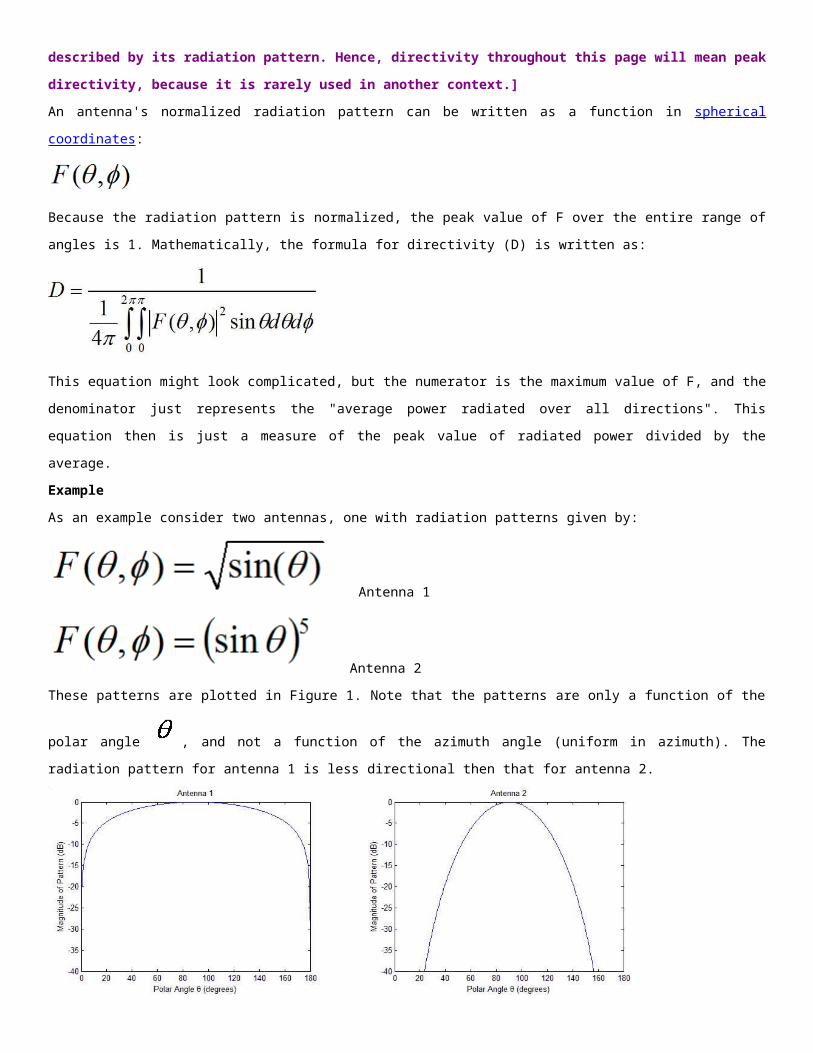
As an example consider two antennas, one with radiation patterns given by:

    Antenna 1

    Antenna 2

These patterns are plotted in Figure 1. Note that the patterns are only a function of the polar angle ,

and not a function of the azimuth angle (uniform in azimuth). The radiation pattern for antenna 1 is less

directional then that for antenna 2.

Figure 1. Plots of Radiation Patterns

The directivity is calculated for Antenna 1 to be 1.273 (1.05 dB).

The directivity is calculated for Antenna 2 to be 2.707 (4.32 dB).

Again, increased directivity implies a more 'focused' antenna. In words, Antenna 2 receives 2.707 times

more power in its peak direction than an isotropic antenna would receive.

Antennas for cell phones should have a low directivity because the signal can come from any direction,

and the antenna should pick it up. In contrast, satellite dish antennas have a very high directivity, because

they are to receive signals from a fixed direction. As an example, if you get a directTV dish, they will tell

you where to point it such that the antenna will receive the signal.

Finally, we'll conclude with a list of antenna types and their directivities, to give you an idea of what is

seen in practice.

Antenna Type Typical Directivity Typical Directivity (dB)

Short Dipole 1.5 1.76

Half Wave Dipole 1.64 2.15

Patch (Microstrip) Antenna 3.2-6.3 5-8

Horn Antenna 10-100 10-20

Dish Antenna 10-10,000 10-40

Antenna Efficiency and Gain: The efficiency of an antenna relates the power delivered to the antenna

and the power radiated or dissipated within the antenna. A high efficiency antenna has most of the power

present at the antenna's input radiated away. A low efficiency antenna has most of the power absorbed as

losses within the antenna.

The losses associated with in an antenna are typically the conduction losses (due to finite conductivity of

the antenna) and dielectric losses (due to conduction within a dielectric which may be present within an

antenna). Sometimes efficiency is defined to also include the mismatch between an antenna and the

transmission line, but this will be discussed in the section on impedance.

The efficiency can be written as the ratio of the radiated power to the input power of the antenna

The term Gain describes how much power is transmitted in the direction of peak radiation to that of an

isotropic source. Gain is more commonly quoted in a real antenna's specification sheet because it takes

into account the actual losses that occur.

A gain of 3 dB means that the power received far from the antenna will be 3 dB (twice as much) higher

than what would be received from a lossless isotropic antenna with the same input power.

Gain is sometimes discussed as a function of angle, but when a single number is quoted the gain is the

'peak gain' over all directions. Gain (G) can be related to directivity (D) by:

The gain of a real antenna can be as high as 40-50 dB for very large dish antennas (although this is rare).

Directivity can be as low as 1.76 dB for a real antenna, but can never theoretically be less than 0 dB.

However the peak gain of an antenna can be arbitrarily low because of losses. Electrically small antennas

(small relative to the wavelength of the frequency that the antenna operates at) can be very inefficient,

with gains lower than -10 dB (even without accounting for impedance mismatch loss)

Beamwidths and Sidelobe Levels: In addition to directivity, radiation patterns of antennas are also

characterized by their beamwidths and sidelobe levels (if applicable).

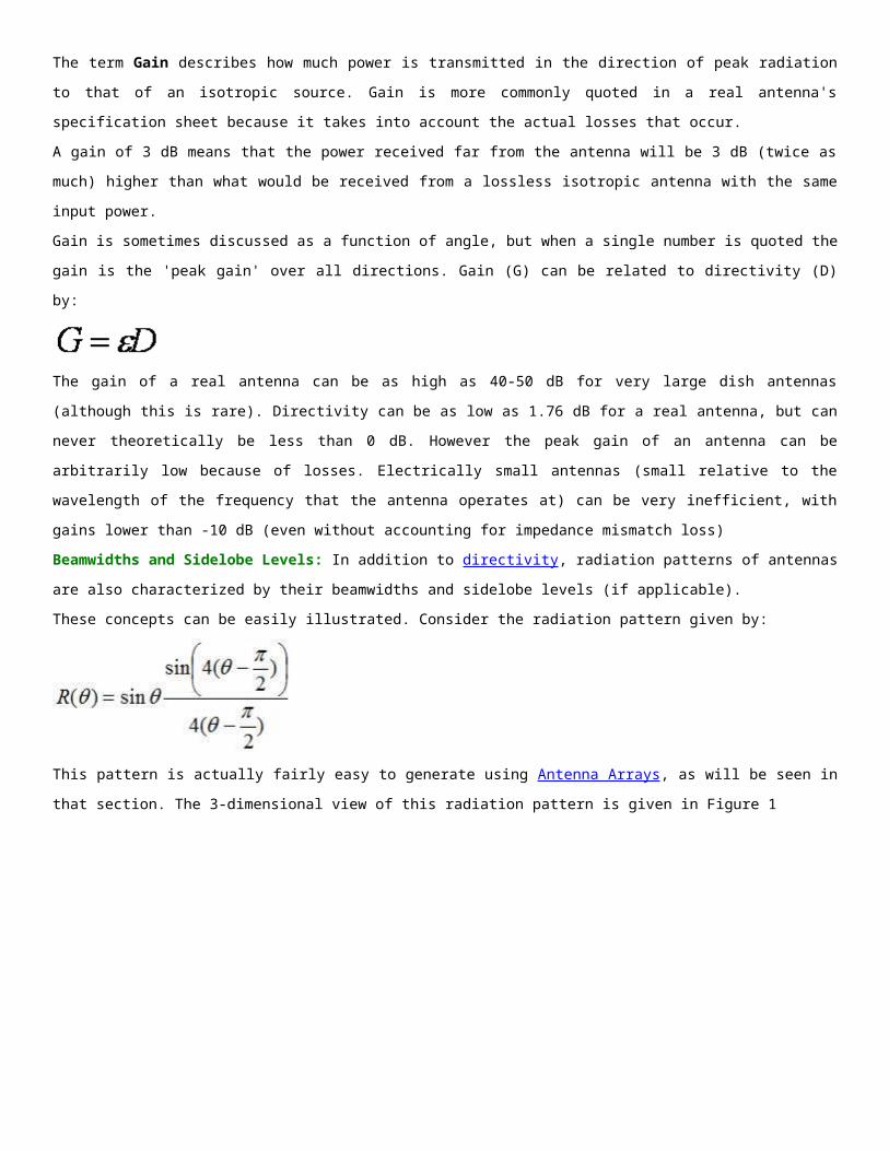
These concepts can be easily illustrated. Consider the radiation pattern given by:

This pattern is actually fairly easy to generate using Antenna Arrays, as will be seen in that section. The 3-

dimensional view of this radiation pattern is given in Figure 1

Figure 1. 3D Radiation Pattern.

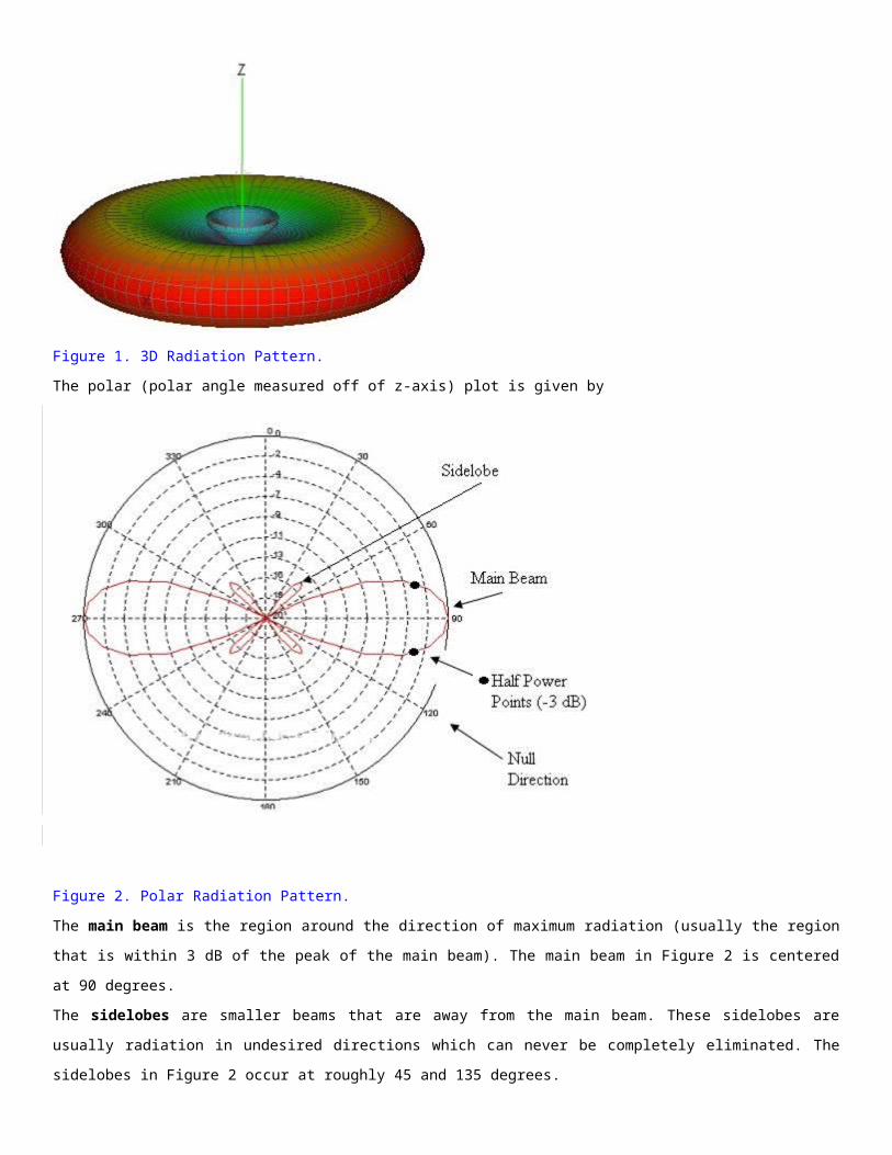
The polar (polar angle measured off of z-axis) plot is given by

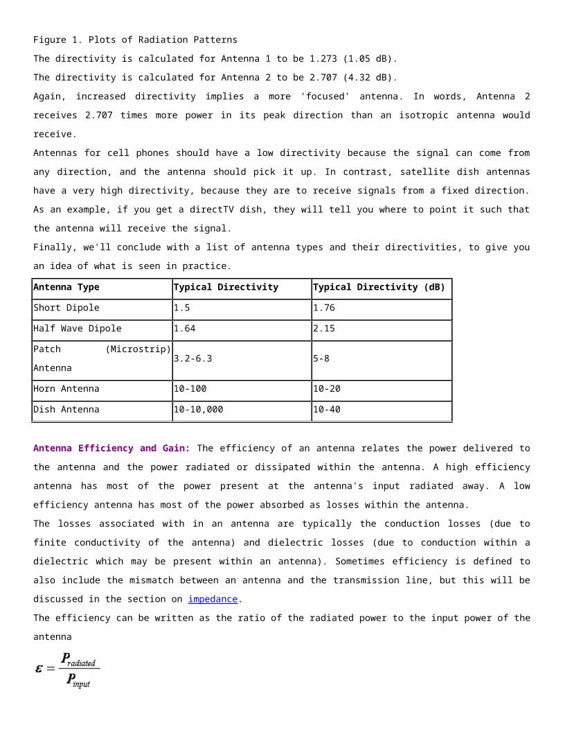
Figure 2. Polar Radiation Pattern.

The main beam is the region around the direction of maximum radiation (usually the region that is within

3 dB of the peak of the main beam). The main beam in Figure 2 is centered at 90 degrees.

The sidelobes are smaller beams that are away from the main beam. These sidelobes are usually

radiation in undesired directions which can never be completely eliminated. The sidelobes in Figure 2

occur at roughly 45 and 135 degrees.

The Half Power Beamwidth (HPBW) is the angular separation in which the magnitude of the radiation

pattern decrease by 50% (or -3 dB) from the peak of the main beam. From Figure 2, the pattern decreases

to -3 dB at 77.7 and 102.3 degrees. Hence the HPBW is 102.3-77.7 = 24.6 degrees.

Another commonly quoted beamwidth is the Null to Null Beamwidth. This is the angular separation from

which the magnitude of the radiation pattern decreases to zero (negative infinity dB) away from the main

beam. From Figure 2, the pattern goes to zero (or minus infinity) at 60 degrees and 120 degrees. Hence,

the Null-Null Beamwidth is 120-60=60 degrees.

Finally, the Sidelobe Level is another important parameter used to characterize radiation patterns. The

sidelobe level is the maximum value of the sidelobes (away from the main beam). From Figure 2, the

Sidelobe Level (SLL) is -14.5 dB

Impedance: An antenna's impedance relates the voltage to the current at the input to the antenna. This

is extremely important as we will see.

Let's say an antenna has an impedance of 50 ohms. This means that if a sinusoidal voltage is input at the

antenna terminals with amplitude 1 Volt, the current will have an amplitude of 1/50 = 0.02 Amps. Since

the impedance is a real number, the voltage is in-phase with the current.

Let's say the impedance is given as Z=50 + j*50 ohms (where j is the square root of -1). Then the

impedance has a magnitude of

and a phase given by

This means the phase of the current will lag the voltage by 45 degrees. To spell it out, if the voltage (with

frequency f) at the antenna terminals is given by

then the current will be given by

So impedance is a simple concept, which relates the voltage and current at the input to the antenna. The

real part of an antenna's impedance represents power that is either radiated away or absorbed within the

antenna. The imaginary part of the impedance represents power that is stored in the near field of the

antenna (non-radiated power). An antenna with a real input impedance (zero imaginary part) is said to be

resonant. Note that an antenna's impedance will vary with frequency.

While simple, we will now explain why this is important, considering both the low frequency and high

frequency cases

Low Frequency

When we are dealing with low frequencies, the transmission line that connects the transmitter or receiver

to the antenna is short. Short in antenna theory always means "relative to a wavelength". Hence, 5 meters

could be short or very long, depending on what frequency we are operating at. At 60 Hz, the wavelength is

about 3100 miles, so the transmission line can almost always be neglected. However, at 2 GHz, the

wavelength is 15 cm, so the little length of line within your cell phone can often be considered a 'long line'.

Basically, if the line length is less than a tenth of a wavelength, it is reasonably considered a short line.

Consider an antenna (which is represented as an impedance given by ZA) hooked up to a voltage source

(of magnitude V) with source impedance given by ZS. The equivalent circuit of this is shown in Figure 1

Figure 1. Circuit model of an antenna hooked to a source.

The power that is delivered to the antenna can be easily found to be (recall your circuit theory, and that

P=I*V):

If ZA is much smaller in magnitude than ZS, then no power will be delivered to the antenna and it won't

transmit or receive energy. If ZA is much larger in magnitude than ZS, then no power will be delivered as

well.

For maximum power to be transferred from the generator to the antenna, the ideal value for the antenna

impedance is given by:

The * in the above equation represents complex conjugate. So if ZS=30+j*30 ohms, then for maximum

power transfer the antenna should impedance ZA=30-j*30 ohms. Typically, the source impedance is real

(imaginary part equals zero), in which case maximum power transfer occurs when ZA=ZS. Hence, we now

know that for an antenna to work properly, its impedance must not be too large or too small. It turns out

that this is one of the fundamental design parameters for an antenna, and it isn't always easy to design an

antenna with the right impedance

High Frequency

This section will be a little more advanced. In low-frequency circuit theory, the wires that connect things

don't matter. Once the wires become a significant fraction of a wavelength, they make things very

different. For instance, a short circuit has an impedance of zero ohms. However, if the impedance is

measured at the end of a quarter wavelength transmission line, the impedance appears to be infinite, even

though there is a dc conduction path.

In general, the transmission line will transform the impedance of an antenna, making it very difficult to

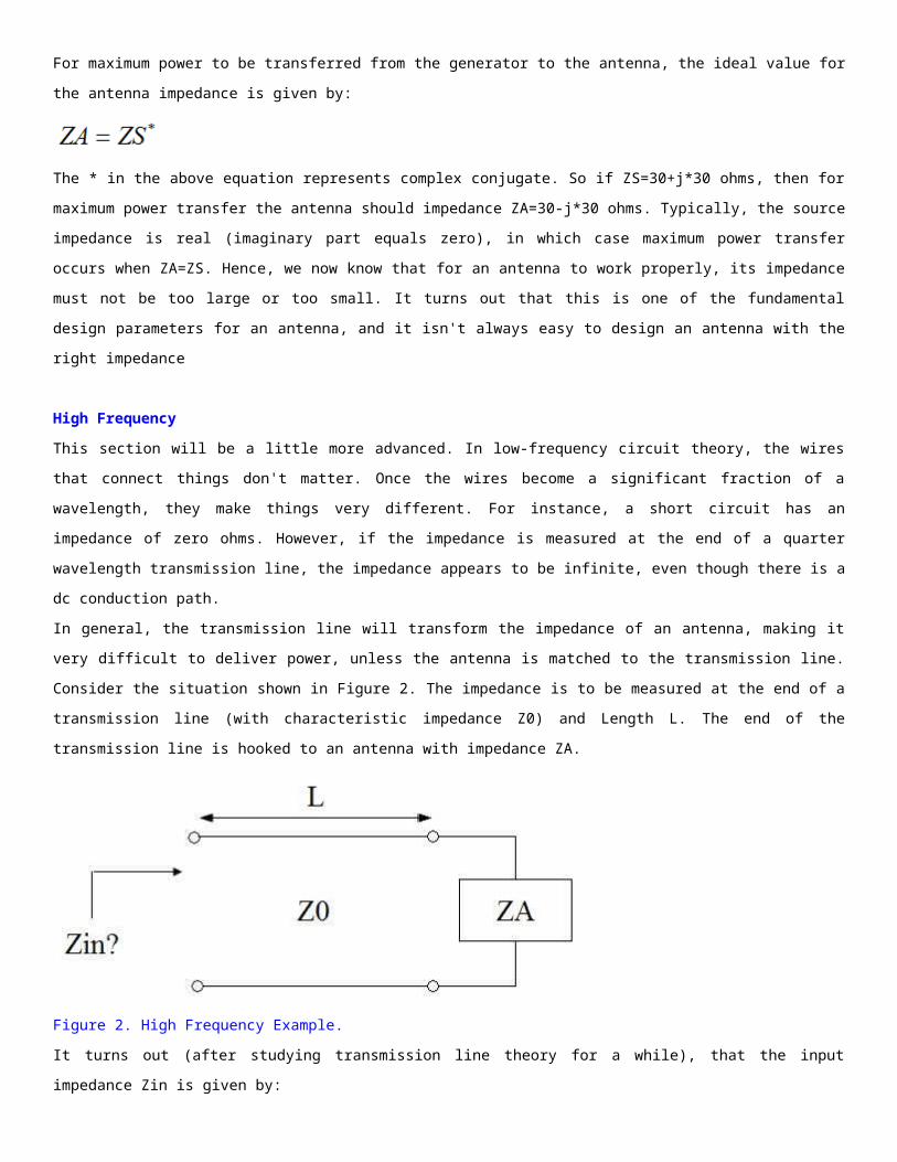
deliver power, unless the antenna is matched to the transmission line. Consider the situation shown in

Figure 2. The impedance is to be measured at the end of a transmission line (with characteristic

impedance Z0) and Length L. The end of the transmission line is hooked to an antenna with impedance ZA.

Figure 2. High Frequency Example.

It turns out (after studying transmission line theory for a while), that the input impedance Zin is given by:

This is a little formidable for an equation to understand at a glance. However, the happy thing is:

If the antenna is matched to the transmission line (ZA=ZO), then the input impedance does

not depend on the length of the transmission line.

Bandwidth: Bandwidth is another fundamental antenna parameter. This describes the range of

frequencies over which the antenna can properly radiate or receive energy. Often, the desired bandwidth

is one of the determining parameters used to decide upon an antenna. For instance, many antenna types

have very narrow bandwidths and cannot be used for wideband operation.

Bandwidth is typically quoted in terms of VSWR. For instance, an antenna may be described as operating

at 100-400 MHz with a VSWR<1.5. This statement implies that the reflection coefficient is less than 0.2

across the quoted frequency range. Hence, of the power delivered to the antenna, only 4% of the power is

reflected back to the transmitter. Alternatively, the return loss S11=20*log10(0.2)=-13.98 dB.

Note that the above does not imply that 96% of the power delivered to the antenna is transmitted in the

form of EM radiation; losses must still be taken into account.

Also, the radiation pattern will vary with frequency. In general, the shape of the radiation pattern does not

change radically.

There are also other criteria which may be used to characterize bandwidth. This may be the polarization

over a certain range, for instance, an antenna may be described as having circular polarization with an

axial ratio <3dB from 1.4-1.6 GHz. This polarization bandwidth sets the range over which the antenna's

operation is roughly circular.

The bandwidth is often specified in terms of its Fractional Bandwidth (FBW). The antenna Q also relates to

bandwidth

Fractional Bandwidth (FBW): The fractional bandwidth of an antenna is a measure of how wideband the

antenna is. If the antenna operates at center frequency fc between lower frequency f1 and upper

frequency f2 (where fc=(f1+f2)/2), then the fractional bandwidth FBW is given by:

The fractional bandwidth varies between 0 and 2, and is often quoted as a percentage (between 0% and

200%). The higher the percentage, the wider the bandwidth.

Wideband antennas typically have a Fractional Bandwidth of 20% or more. Antennas with a FBW of greater

than 50% are referred to as ultra-wideband antennas.

Polarization: Polarization is one of the fundamental characteristics of any antenna. First we'll need to

understand polarization of plane waves, then We'll walk through the main types of polarization.

Linear Polarization

Let's start by understanding the polarization of a wave.

A plane electromagnetic (EM) wave is characterized by travelling in a single direction (with no field

variation in the two orthogonal directions). In this case, the electric field and the magnetic field are

perpendicular to each other and to the direction the plane wave is propagating. As an example, consider

the single frequency E-field given by equation (1), where the field is traveling in the +z-direction, the E-

field is oriented in the +x-direction, and the magnetic field is in the +y-direction.

In equation (1), the symbol is a unit vector (a vector with a length of one), which says that the E-field

"points" in the x-direction.

A plane wave is illustrated graphically in Figure 1.

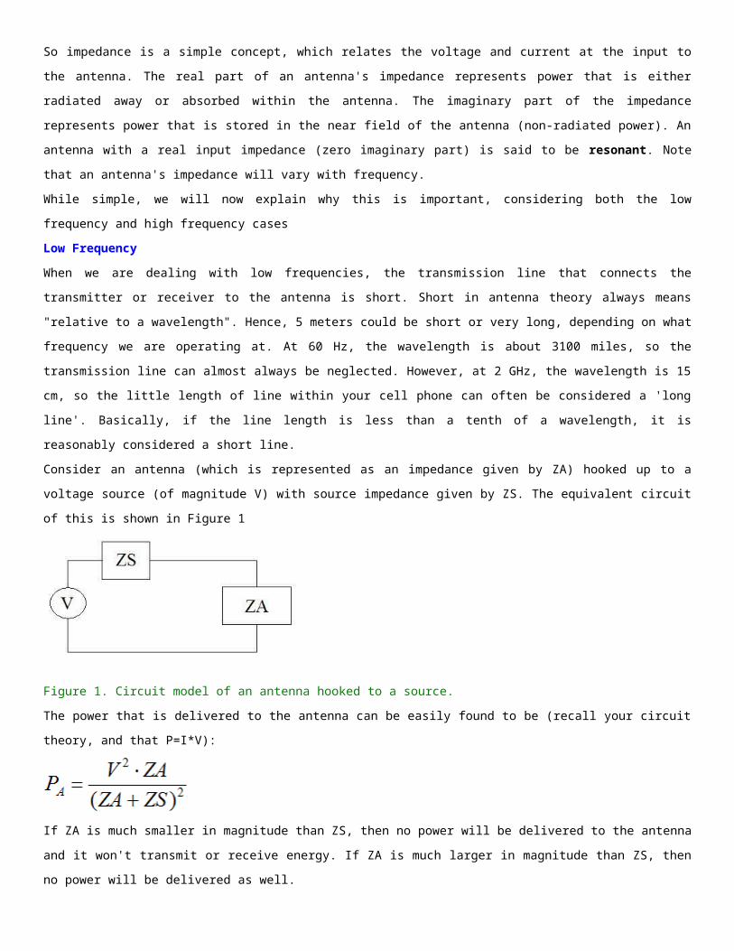
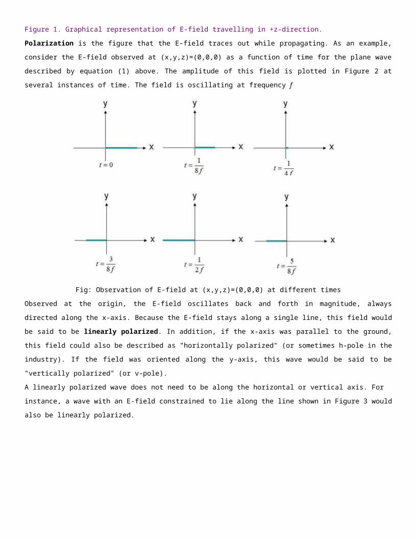
Figure 1. Graphical representation of E-field travelling in +z-direction.

Polarization is the figure that the E-field traces out while propagating. As an example, consider the E-field

observed at (x,y,z)=(0,0,0) as a function of time for the plane wave described by equation (1) above. The

amplitude of this field is plotted in Figure 2 at several instances of time. The field is oscillating at frequency

f

Fig: Observation of E-field at (x,y,z)=(0,0,0) at different times

Observed at the origin, the E-field oscillates back and forth in magnitude, always directed along the x-axis.

Because the E-field stays along a single line, this field would be said to be linearly polarized. In addition,

if the x-axis was parallel to the ground, this field could also be described as "horizontally polarized" (or

sometimes h-pole in the industry). If the field was oriented along the y-axis, this wave would be said to be

"vertically polarized" (or v-pole).

A linearly polarized wave does not need to be along the horizontal or vertical axis. For instance, a wave

with an E-field constrained to lie along the line shown in Figure 3 would also be linearly polarized.

Figure 3. Locus of E-field amplitudes for a linearly polarized wave at an angle.

The E-field in Figure 3 could be described by equation (2). The E-field now has an x- and y- component,

equal in magnitude.

One thing to notice about equation (2) is that the x- and y-components of the E-field are in phase - they

both have the same magnitude and vary at the same rate.

Circular Polarization

Suppose now that the E-field of a plane wave was given by equation (3):

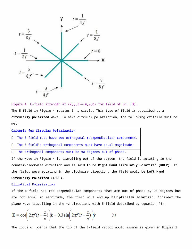
In this case, the x- and y- components are 90 degrees out of phase. If the field is observed at

(x,y,z)=(0,0,0) again as before, the plot of the E-field versus time would appear as shown in Figure 4

Figure 4. E-field strength at (x,y,z)=(0,0,0) for field of Eq. (3).

The E-field in Figure 4 rotates in a circle. This type of field is described as a circularly polarized wave. To

have circular polarization, the following criteria must be met.

Criteria for Circular Polarization

The E-field must have two orthogonal (perpendicular) components.

The E-field's orthogonal components must have equal magnitude.

The orthogonal components must be 90 degrees out of phase.

If the wave in Figure 4 is travelling out of the screen, the field is rotating in the counter-clockwise direction

and is said to be Right Hand Circularly Polarized (RHCP). If the fields were rotating in the clockwise

direction, the field would be Left Hand Circularly Polarized (LHCP).

Elliptical Polarization

If the E-field has two perpendicular components that are out of phase by 90 degrees but are not equal in

magnitude, the field will end up Elliptically Polarized. Consider the plane wave travelling in the +z-

direction, with E-field described by equation (4):

The locus of points that the tip of the E-field vector would assume is given in Figure 5

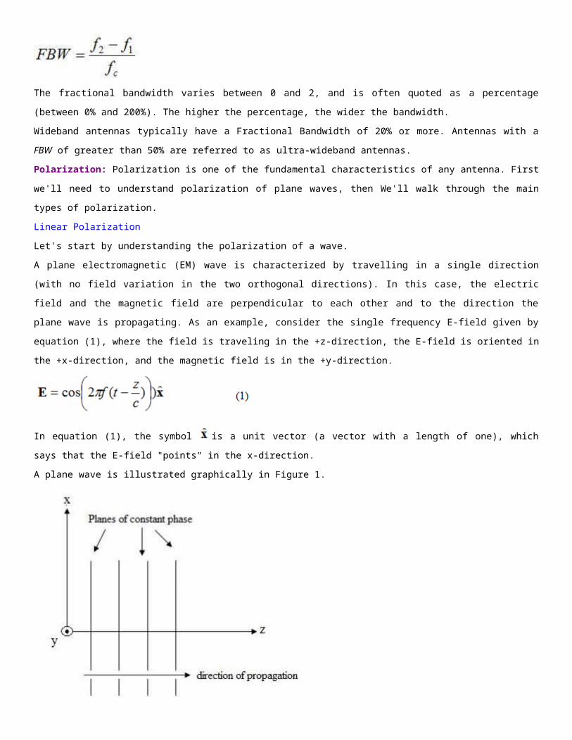
Figure 5. Tip of E-field for elliptical polarized wave of Eq. (4).

The field in Figure 5, travels in the counter-clockwise direction, and if travelling out of the screen would be

Right Hand Elliptically Polarized. If the E-field vector was rotating in the opposite direction, the field

would be Left Hand Elliptically Polarized.

In addition, elliptical polarization is defined by its eccentricity, which is the ratio of the major and minor

axis amplitudes. For instance, the eccentricity of the wave given by equation (4) is 1/0.3 = 3.33. Elliptically

polarized waves are further described by the direction of the major axis. The wave of equation (4) has a

major axis given by the x-axis. Note that the major axis can be at any angle in the plane, it does not need

to coincide with the x-, y-, or z-axis. Finally, note that circular polarization and linear polarization are both

special cases of elliptical polarization. An elliptically polarized wave with an eccentricity of 1.0 is a

circularly polarized wave; an elliptically polarized wave with an infinite eccentricity is a linearly polarized

wave

Antenna Polarization: The polarization of an antenna is the polarization of the radiated fields produced

by an antenna, evaluated in the far field. Hence, antennas are often classified as "Linearly Polarized" or a

"Right Hand Circularly Polarized Antenna".

This simple concept is important for antenna to antenna communication. First, a horizontally polarized

antenna will not communicate with a vertically polarized antenna. Due to the reciprocity theorem,

antennas transmit and receive in exactly the same manner. Hence, a vertically polarized antenna

transmits and receives vertically polarized fields. Consequently, if a horizontally polarized antenna is trying

to communicate with a vertically polarized antenna, there will be no reception.

In general, for two linearly polarized antennas that are rotated from each other by an angle , the power

loss due to this polarization mismatch will be described by the Polarization Loss Factor (PLF):

Hence, if both antennas have the same polarization, the angle between their radiated E-fields is zero and

there is no power loss due to polarization mismatch. If one antenna is vertically polarized and the other is

horizontally polarized, the angle is 90 degrees and no power will be transferred.

As a side note, this explains why moving the cell phone on your head to a different angle can sometimes

increase reception. Cell phone antennas are often linearly polarized, so rotating the phone can often

match the polarization of the phone and thus increase reception.

Circular polarization is a desirable characteristic for many antennas. Two antennas that are both circularly

polarized do not suffer signal loss due to polarization mismatch. Antennas used in GPS systems are Right

Hand Circularly Polarized.

Suppose now that a linearly polarized antenna is trying to receive a circularly polarized wave. Equivalently,

suppose a circularly polarized antenna is trying to receive a linearly polarized wave. What is the resulting

Polarization Loss Factor?

Recall that circular polarization is really two orthongal linear polarized waves 90 degrees out of phase.

Hence, a linearly polarized (LP) antenna will simply pick up the in-phase component of the circularly

polarized (CP) wave. As a result, the LP antenna will have a polarization mismatch loss of 0.5 (-3dB), no

matter what the angle the LP antenna is rotated to. Therefore:

The Polarization Loss Factor is sometimes referred to as polarization efficiency, antenna mismatch factor,

or antenna receiving factor. All of these names refer to the same concept

Effective Area: A useful parameter calculating the receive power of an antenna is the effective area or

effective aperture. Assume that a plane wave with the same polarization as the receive antenna is incident

upon the antenna. Further assume that the wave is travelling towards the antenna in the antenna's

direction of maximum radiation (the direction from which the most power would be received).

Then the effective aperture parameter describes how much power is captured from a given plane wave.

Let W be the power density of the plane wave (in W/m^2). If P represents the power at the antennas

terminals available to the antenna's receiver, then:

Hence, the effective area simply represents how much power is captured from the plane wave and

delivered by the antenna. This area factors in the losses intrinsic to the antenna (ohmic losses, dielectric

losses, etc.). This parameter can be determine by measurement for real antennas.

A general relation for the effective aperture in terms of the peak gain (G) of any antenna is given by:

Effective aperture will be a useful concept for calculating received power from a plane wave. To see this in

action, go to the next section on the Friis transmission formula.

Friis Transmission Formula: This page is worth reading a couple times and should be fully understood.

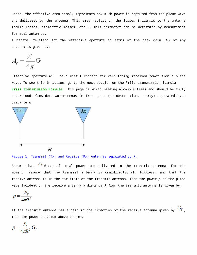
Consider two antennas in free space (no obstructions nearby) separated by a distance R:

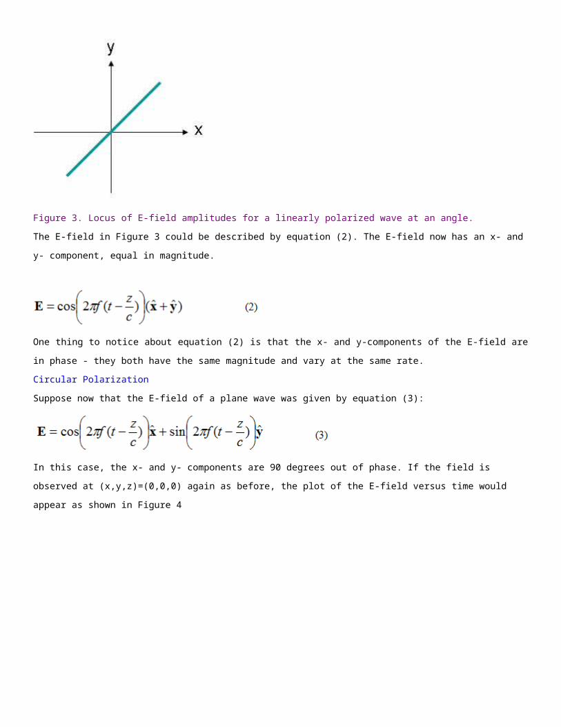
Figure 1. Transmit (Tx) and Receive (Rx) Antennas separated by R.

Assume that Watts of total power are delivered to the transmit antenna. For the moment, assume that

the transmit antenna is omnidirectional, lossless, and that the receive antenna is in the far field of the

transmit antenna. Then the power p of the plane wave incident on the receive antenna a distance R from

the transmit antenna is given by:

If the transmit antenna has a gain in the direction of the receive antenna given by , then the power

equation above becomes:

The gain term factors in the directionality and losses of a real antenna. Assume now that the receive

antenna has an effective aperture given by . Then the power received by this antenna ( ) is given

by:

Since the effective aperture for any antenna can also be expressed as:

The resulting received power can be written as:

This is known as the Friis Transmission Formula. It relates the free space path loss, antenna gains and

wavelength to the received and transmit powers. This is one of the fundamental equations in antenna

theory, and should be remembered (as well as the derivation above).

Finally, if the antennas are not polarization matched, the above received power could be multiplied by the

Polarization Loss Factor (PLF) to properly account for this mismatch

Antenna Temperature: Antenna Temperature ( ) is a parameter that describes how much noise an

antenna produces in a given environment. This temperature is not the physical temperature of the

antenna. Moreover, an antenna does not have an intrinsic "antenna temperature" associated with it; rather

the temperature depends on its gain pattern and the thermal environment that it is placed in.

To define the environment, we'll introduce a temperature distribution - this is the temperature in every

direction away from the antenna in spherical coordinates. For instance, the night sky is roughly 4 Kelvin;

the value of the temperature pattern in the direction of the Earth's ground is the physical temperature of

the Earth's ground. This temperature distribution will be written as . Hence, an antenna's

temperature will vary depending on whether it is directional and pointed into space or staring into the sun.

For an antenna with a radiation pattern given by , the noise temperature is mathematically defined

as:

This states that the temperature surrounding the antenna is integrated over the entire sphere, and

weighted by the antenna's radiation pattern. Hence, an isotropic antenna would have a noise temperature

that is the average of all temperatures around the antenna; for a perfectly directional antenna (with a

pencil beam), the antenna temperature will only depend on the temperature in which the antenna is

"looking".

The noise power received from an antenna at temperature can be expressed in terms of the bandwidth

(B) the antenna (and its receiver) are operating over:

In the above, K is Boltzmann's constant (1.38 * 10^-23 [Joules/Kelvin = J/K]). The receiver also has a

temperature associated with it ( ), and the total system temperature (antenna plus receiver) has a

combined temperature given by . This temperature can be used in the above equation to

find the total noise power of the system. These concepts begin to illustrate how antenna engineers must

understand receivers and the associated electronics, because the resulting systems very much depend on

each other.

A parameter often encountered in specification sheets for antennas that operate in certain environments is

the ratio of gain of the antenna divided by the antenna temperature (or system temperature if a receiver is

specified). This parameter is written as G/T, and has units of dB/Kelvin [dB/K]

Why do Antennas Radiate?: Obtaining an intuitive idea for why antennas radiate is helpful in

understanding the fundamentals of antennas. On this page, I'll attempt to give a low-key explanation with

no regard to mathematics on how and why antennas radiate electromagnetic fields.

First, lets start with some basic physics. There is electric charge - this is a quantity of nature (like mass or

weight or density) that every object possesses. You and I are most likely electrically neutral - we don't

have a net charge that is positive or negative. There exists in every atom in the universe particles that

contain positive and negative charge (protons and electrons, respectively). Some materials (like metals)

that are very electrically conductive have loosely bound electrons. Hence, when a voltage is applied across

a metal, the electrons travel around a circuit - this flow of electrons is electric current (measured in Amps).

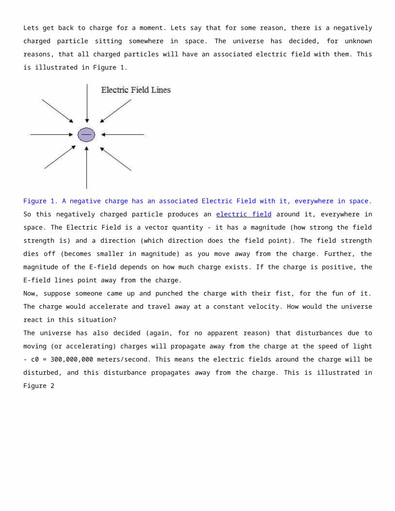
Lets get back to charge for a moment. Lets say that for some reason, there is a negatively charged particle

sitting somewhere in space. The universe has decided, for unknown reasons, that all charged particles will

have an associated electric field with them. This is illustrated in Figure 1.

Figure 1. A negative charge has an associated Electric Field with it, everywhere in space.

So this negatively charged particle produces an electric field around it, everywhere in space. The Electric

Field is a vector quantity - it has a magnitude (how strong the field strength is) and a direction (which

direction does the field point). The field strength dies off (becomes smaller in magnitude) as you move

away from the charge. Further, the magnitude of the E-field depends on how much charge exists. If the

charge is positive, the E-field lines point away from the charge.

Now, suppose someone came up and punched the charge with their fist, for the fun of it. The charge would

accelerate and travel away at a constant velocity. How would the universe react in this situation?

The universe has also decided (again, for no apparent reason) that disturbances due to moving (or

accelerating) charges will propagate away from the charge at the speed of light - c0 = 300,000,000

meters/second. This means the electric fields around the charge will be disturbed, and this disturbance

propagates away from the charge. This is illustrated in Figure 2

Figure 2. The E-fields when the charge is accelerated.

Once the charge is accelerated, the fields need to re-align themselves. Remember, the fields want to

surround the charge exactly as they did in Figure 1. However, the fields can only respond to events at the

speed of light. Hence, if a point is very far away from the charge, it will take time for the disturbance (or

change in electric fields) to propagate to the point. This is illustrated in Figure 2.

In Figure 2, we have 3 regions. In the light blue (inner) region, the fields close to the charge have

readapted themselves and now line up as they do in Figure 1. In the white region (outermost), the fields

are still undisturbed and have the same magnitude and direction as they would if the charge had not

moved. In the pink region, the fields are changing - from their old magnitude and direction to their new

magnitude and direction.

Hence, we have arrived at the fundamental reason for radiation - the fields change because charges are

accelerated. The fields always try to align themselves as in Figure 1 around charges. If we can produce a

moving set of charges (this is simply electric current), then we will have radiation

Wire Antennas

Short Dipole

Dipole Antenna

Half-Wave Dipole

Broadband Dipoles

Monopole

Folded Dipole

Small Loop

Microstrip Antennas

Rectangular Microstrip (Patch) Antenna

Shorting Pins: Quarter-Wavelength Microstrips and PIFAs

Reflector Antennas

Corner Reflector

Parabolic Reflector (Dish Antenna)

Travelling Wave Antennas

Helical Antenna

Yagi-Uda Antenna

Aperture Antennas

Slot Antenna

Cavity-Backed Slot Antenna

Inverted-F Antenna

Slotted Waveguide Antenna

Horn Antenna

The Short Dipole Antenna: The short dipole antenna is the simplest of all antennas. It is simply an open-

circuited wire, fed at its center as shown in Figure 1.

Figure 1. Short dipole antenna of length L.

The words "short" or "small" in antenna engineering always imply "relative to a wavelength". So the

absolute size of the above dipole does not matter, only the size of the wire relative to the wavelength of

the frequency of operation. Typically, a dipole is short if its length is less than a tenth of a wavelength:

If the antenna is oriented along the z-axis with the center of the dipole at z=0, then the current distribution

on a thin, short dipole is given by:

The current distribution is plotted in Figure 2. Note that this is the amplitude of the current distribution; it

is oscillating in time sinusoidally at frequency f.

Figure 2. Current distribution along a short dipole.

The fields radiated from this antenna in the far field are given by:

The above equations can be broken down and understood somewhat intuitively. First, note that in the far-

field, only the and fields are nonzero. Further, these fields are orthogonal and in-phase. Further,

the fields are perpendicular to the direction of propagation, which is always in the direction (away from

the antenna). Also, the ratio of the E-field to the H-field is given by (the intrinsic impedance of free

space). This indicates that in the far-field region the fields are propagating like a plane-wave.

Second, the fields die off as 1/r, which indicates the power falls of as

Third, the fields are proportional to L, indicated a longer dipole will radiate more power. This is true as long

as increasing the length does not cause the short dipole assumption to become invalid. Also, the fields are

proportional to the current amplitude , which should make sense (more current, more power).

The exponential term:

describes the phase-variation of the wave versus distance. Note also that the fields are oscillating in time

at a frequency f in addition to the above spatial variation.

Finally, the spatial variation of the fields as a function of direction from the antenna are given by .

For a vertical antenna oriented along the z-axis, the radiation will be maximum in the x-y plane.

Theoretically, there is no radiation along the z-axis far from the antenna.

The directivity of the center-fed short dipole antenna depends only on the component of

the fields. It can be calculated to be 1.5 (1.76 dB), which is very low for realizable antennas. Since the

fields are only a function of the polar angle, they have no azimuthal variation and hence this antenna is

characterized as omnidirectional. The Half-Power Beamwidth is 90 degrees.

The polarization of this antenna is linear. When evaluated in the x-y plane, this antenna would be

described as vertically polarized, because the E-field would be vertically oriented (along the z-axis).

We now turn to the input impedance of the short dipole, which depends on the radius a of the dipole.

Recall that the impedance Z is made up of three components, the radiation resistance, the loss resistance,

and the reactive (imaginary) component which represents stored energy in the fields:

The radiation resistance can be calculated to be:

The resistance representing loss due to the finite-conductivity of the antenna is given by:

In the above equation represents the conductivity of the dipole (usually very high, if made of metal).

The frequency f come into the above equation because of the skin effect. The reactance or imaginary part

of the impedance of a dipole is roughly equal to:

As an example, assume that the radius is 0.001 and the length is 0.05 . Suppose further that this

antenna is to operate at f=3 MHz, and that the metal is copper, so that the conductivity is 59,600,000 S/m.

The radiation resistance is calculated to be 0.49 Ohms. The loss resistance is found to be 4.83 mOhms

(milli-Ohms), which is approximatley negligible when compared to the radiation resistance. However, the

reactance is 1695 Ohms, so that the input resistance is Z=0.49 + j1695. Hence, this antenna would be

very difficult to have proper impedance matching. Even if the reactance could be properly cancelled out,

very little power would be delivered from a 50 Ohm source to a 0.49 Ohm load.

For short dipoles that are smaller fractions of a wavelength, the radiation resistance becomes smaller than

the loss resistance, and consequently this antenna can be very inefficient.

The bandwidth for short dipoles is difficult to define. The input impedance varies wildly with frequency

because of the reactance component of the input impedance. Hence, these antennas are typically used in

narrowband applications.

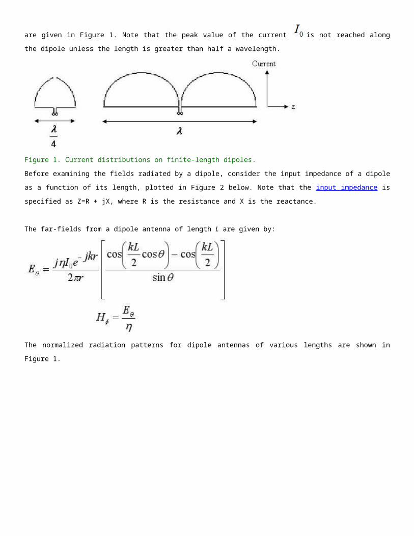
The Dipole Antenna: In this section, the dipole antenna with a very thin radius is considered. The dipole

is similar to the short dipole except it is not required to be small compared to the wavelength (of the

frequency the antenna is operating at).

For a dipole antenna of length L oriented along the z-axis and centered at z=0, the current flows in the z-

direction with amplitude which closely follows the following function:

Note that this current is also oscillating in time sinusoidally at frequency f. The current distributions for a

quarter-wavelength (left) and full-wavelength (right) dipoles are given in Figure 1. Note that the peak

value of the current is not reached along the dipole unless the length is greater than half a

wavelength.

Figure 1. Current distributions on finite-length dipoles.

Before examining the fields radiated by a dipole, consider the input impedance of a dipole as a function of

its length, plotted in Figure 2 below. Note that the input impedance is specified as Z=R + jX, where R is

the resistance and X is the reactance.

The far-fields from a dipole antenna of length L are given by:

The normalized radiation patterns for dipole antennas of various lengths are shown in Figure 1.

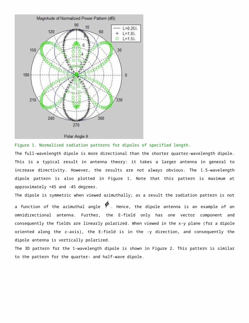
Figure 1. Normalized radiation patterns for dipoles of specified length.

The full-wavelength dipole is more directional than the shorter quarter-wavelength dipole. This is a typical

result in antenna theory: it takes a larger antenna in general to increase directivity. However, the results

are not always obvious. The 1.5-wavelength dipole pattern is also plotted in Figure 1. Note that this pattern

is maximum at approximately +45 and -45 degrees.

The dipole is symmetric when viewed azimuthally; as a result the radiation pattern is not a function of the

azimuthal angle . Hence, the dipole antenna is an example of an omnidirectional antenna. Further, the

E-field only has one vector component and consequently the fields are linearly polarized. When viewed in

the x-y plane (for a dipole oriented along the z-axis), the E-field is in the -y direction, and consequently the

dipole antenna is vertically polarized.

The 3D pattern for the 1-wavelength dipole is shown in Figure 2. This pattern is similar to the pattern for

the quarter- and half-wave dipole.

Figure 2. Normalized 3d radiation pattern for the 1-wavelength dipole.

The 3D radiation pattern for the 1.5-wavelength dipole is significantly different, and is shown in Figure 3.

Figure 3. Normalized 3d radiation pattern for the 1.5-wavelength dipole.

The (peak) directivity of the dipole varies as shown in Figure 4.

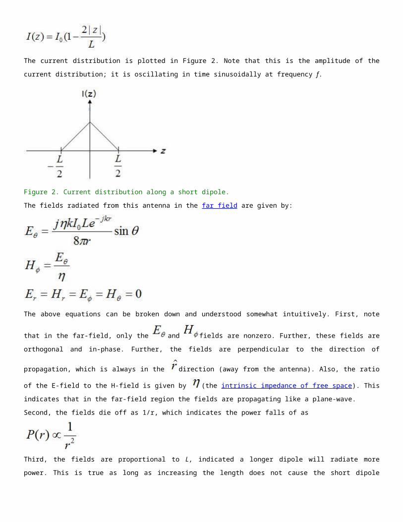
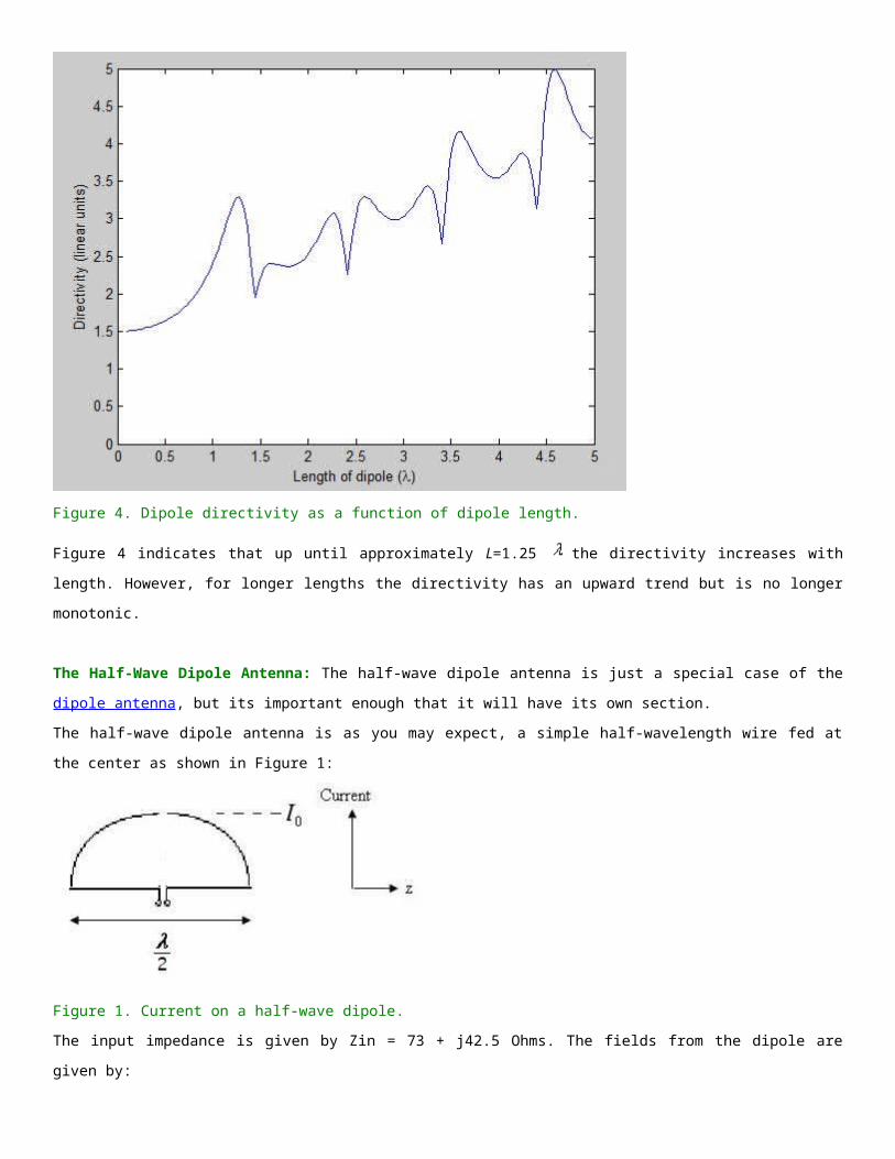
Figure 4. Dipole directivity as a function of dipole length.

Figure 4 indicates that up until approximately L=1.25 the directivity increases with length. However, for

longer lengths the directivity has an upward trend but is no longer monotonic.

The Half-Wave Dipole Antenna: The half-wave dipole antenna is just a special case of the dipole

antenna, but its important enough that it will have its own section.

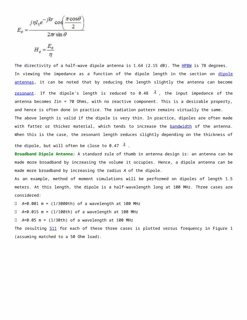
The half-wave dipole antenna is as you may expect, a simple half-wavelength wire fed at the center as

shown in Figure 1:

Figure 1. Current on a half-wave dipole.

The input impedance is given by Zin = 73 + j42.5 Ohms. The fields from the dipole are given by:

The directivity of a half-wave dipole antenna is 1.64 (2.15 dB). The HPBW is 78 degrees.

In viewing the impedance as a function of the dipole length in the section on dipole antennas, it can be

noted that by reducing the length slightly the antenna can become resonant. If the dipole's length is

reduced to 0.48 , the input impedance of the antenna becomes Zin = 70 Ohms, with no reactive

component. This is a desirable property, and hence is often done in practice. The radiation pattern remains

virtually the same.

The above length is valid if the dipole is very thin. In practice, dipoles are often made with fatter or thicker

material, which tends to increase the bandwidth of the antenna. When this is the case, the resonant length

reduces slightly depending on the thickness of the dipole, but will often be close to 0.47 .

Broadband Dipole Antenna: A standard rule of thumb in antenna design is: an antenna can be made

more broadband by increasing the volume it occupies. Hence, a dipole antenna can be made more

broadband by increasing the radius A of the dipole.

As an example, method of moment simulations will be performed on dipoles of length 1.5 meters. At this

length, the dipole is a half-wavelength long at 100 MHz. Three cases are considered:

A=0.001 m = (1/3000th) of a wavelength at 100 MHz

A=0.015 m = (1/100th) of a wavelength at 100 MHz

A=0.05 m = (1/30th) of a wavelength at 100 MHz

The resulting S11 for each of these three cases is plotted versus frequency in Figure 1 (assuming matched

to a 50 Ohm load).

Figure 1. Magnitude of S11 for Dipoles of Varying Radii.

The first thing apparent from Figure 1 is that the fatter the dipole is made, the larger the bandwidth

becomes. For instance, if the bandwidth is measured as the frequency range over which |S11|<-9 dB, then

the bandwidths are 6.5 MHz, 14 MHz, and 24 MHz, for the blue, green and red curves, respectively.

Secondly, the fatter the dipole gets the lower the resonant frequency becomes. In other words, if an

antenna is to resonate at 100 MHz, the resonant length decreases as the dipole gets fatter.

Monopole Antenna: A monopole antenna is one half of a dipole antenna, almost always mounted above

some sort of ground plane. The case of a monopole of length L mounted above an infinite ground plane is

shown in Figure 1(a).

Figure 1. Monopole above a PEC (a), and the equivalent source in free space (b).

Using image theory, the fields above the ground plane can be found by using the equivalent source

(antenna) in free space as shown in Figure 1(b). This is simply a dipole antenna of twice the length. The

fields above the ground plane in Figure 1(a) are identical to the fields in Figure 1(b), which are known and

presented in the dipole section. The fields below the ground plane in Figure 1(a) are zero.

The radiation pattern of monopoles above a ground plane are also known from the dipole result. The only

change that needs to be noted is that the impedance of a monopole is one half of that of a full dipole

antenna. For a quarter-wave monopole (L=0.25* ), the impedance is half of that of a half-wave dipole,

so Zin = 36.5 + j21.25 Ohms. This can be understood since only half the voltage is required to drive a

monopole to the same current as a dipole (think of a dipole as having +V/2 and -V/2 applied to its ends,

whereas a monopole only needs to apply +V/2 between the monopole and the ground to drive the same

current). Since Zin = V/I, the impedance is halved.

The directivity of a monopole antenna is directly related to that of a dipole antenna. If the directivity of a

dipole of length 2L has a directivity of D1 [decibels], then the directivity of a monopole antenna of length L

will have a directivity of D1+3 [decibels]. That is, the directivity (in linear units) of a monopole is twice the

directivity of a dipole antenna of twice the length. The reason for this is simply because no radiation occurs

below the ground plane; hence, the antenna is effectively twice as "directive".

Monopoles are half the size of their dipole counterparts, and hence are attractive when a smaller antenna

is needed. Antennas on older cell phones were typically monopoles, with an infinite ground plane

approximated by a small metal plate below the antenna.

Effects of a Finite Size Ground Plane

In practice, monopoles are used on finite-sized ground planes. This affects the properties of the monopole

antennas. The impedance of a monopole antenna is minimally affected by a finite-sized ground plane for

ground planes of at least a few wavelengths in size around the monopole. However, the radiation pattern

for the monopole is strongly affected by a finite sized ground plane. The resulting radiation pattern

radiates in a "skewed" direction, away from the horizontal plane. An example of the radiation pattern for a

quarter-wavelength monopole antenna (oriented in the +z-direction) on a ground plane with a diameter of

3 wavelengths is shown in the following Figure.

Note that the resulting radiation pattern is still omnidirectional. However, the direction of peak-radiation

has changed from the x-y plane to an angle elevated from that plane. In general, the large the ground

plane is, the lower this direction of maximum radiation; as the ground plane approaches infinite size, the

radiation pattern approaches a maximum in the x-y plane.

The Folded Dipole Antenna: A folded dipole is a dipole antenna, with the ends folded back around and

connected to each other, forming a loop as shown in Figure 1.

Figure 1. Folded dipole of length L.

Typically, the width d of the folded dipole is much smaller than the length L.

Because the dipole is a closed loop, one would expect the input impedance to depend on the input

impedance of a short-circuited transmission line of length L (although unfortunately it depends on a

transmission line of length L/2, which doesn't quite make intuitive sense to me). Also, because the dipole is

folded back on itself, the currents can reinforce each other instead of cancelling each other out, so the

input impedance will also depend on the impedance of a dipole antenna of length L.

Letting Zd represent the impedance of a dipole antenna and Zt represent the transmission line impedance

given by:

The input impedance ZA of the folded dipole is given by:

The folded dipole is resonant and radiates well at odd integer multiples of a half-wavelength (0.5 , 1.5

, ...). The input impedance is higher than that for a regular dipole.

The antenna impedance for a half-wavelength folded dipole antenna can be found from the above

equation for ZA; the result is ZA=4*Zd. At resonance, the impedance of a half-wave dipole antenna is

approximately 70 Ohms, so that the input impedance for a half-wave folded dipole is roughly 280 Ohms.

Because the characteristic impedance of twin-lead transmission lines are roughly 300 Ohms, this dipole is

often used when connecting to this type of line, for optimal power transfer.

The radiation pattern of half-wavelength folded dipoles have the same form as that of half-wavelength

dipoles.

Small Loop Antenna: The small loop antenna is a closed loop as shown in Figure 1. These antennas have

low radiation resistance and high reactance, so that their impedance is difficult to match to a transmitter.

As a result, these antennas are most often used as receive antennas, where impedance mismatch loss can

be tolerated.

The radius is a, and is assumed to be much smaller than a wavelength (a<< ). The loop lies in the x-y

plane.

Figure 1. Small loop antenna.

Since the loop is electrically small, the current within the loop can be approximated as being constant

along the loop, so that I= .

The fields from a small circular loop are given by:

The variation of the pattern with direction is given by , so that the radiation pattern of a small loop

antenna has the same power pattern as that of a short dipole. However, the fields of a small dipole have

the E- and H- fields switched relative to that of a short dipole; the E-field is horizontally polarized in the x-y

plane.

The small loop is often referred to as the dual of the dipole antenna, because if a small dipole had

magnetic current flowing (as opposed to electric current as in a regular dipole), the fields would resemble

that of a small loop.

While the short dipole has a capacitive impedance (imaginary part of impedance is negative), the

impedance of a small loop is inductive (positive imaginary part). The radiation resistance (and ohmic loss

resistance) can be increased by adding more turns to the loop. If there are N turns of a small loop antenna,

each with a surface area S (we don't require the loop to be circular at this point), the radiation resistance

for small loops can be approximated (in Ohms) by:

For a small loop, the reactive component of the impedance can be determined by finding the inductance of

the loop, which depends on its shape (then X=2*pi*f*L). For a circular loop with radius a and wire radius p,

the reactive component of the impedance is given by:

Small loops often have a low radiation resistance and a highly inductive component to their reactance.

Hence, they are most often used as receive antennas. Examples of their use include in pagers, and as field

strength probes used in wireless measurements.

Rectangular Microstrip Antenna: Microstrip or patch antennas are becoming increasingly useful

because they can be printed directly onto a circuit board. They are becoming very widespread within the

mobile phone market. They are low cost, have a low profile and are easily fabricated.

Consider the microstrip antenna shown in Figure 1, fed by a microstrip transmission line. The patch,

microstrip and ground plane are made of high conductivity metal. The patch is of length L, width W, and

sitting on top of a substrate (some dielectric circuit board) of thickness h with permittivity . The

thickness of the ground plane or of the microstrip is not critically important. Typically the height h is much

smaller than the wavelength of operation.

.

(a) Top View

(b) Side View

Figure 1. Geometry of Microstrip (Patch) Antenna.

The frequency of operation of the patch antenna of Figure 1 is determined by the length

L. The center frequency will be approximately given by:

The above equation says that the patch antenna should have a length equal to one half

of a wavelength within the dielectric (substrate) medium.

The width W of the antenna controls the input impedance. For a square patch fed in the

manner above, the input impedance will be on the order of 300 Ohms. By increasing the

width, the impedance can be reduced. However, to decrease the input impedance to 50

Ohms often requires a very wide patch. The width further controls the radiation pattern.

The normalized pattern is approximately given by:

In the above, k is the free-space wavenumber, given by . The magnitude of the

fields, given by:

The fields are plotted in Figure 2 for W=L=0.5 .

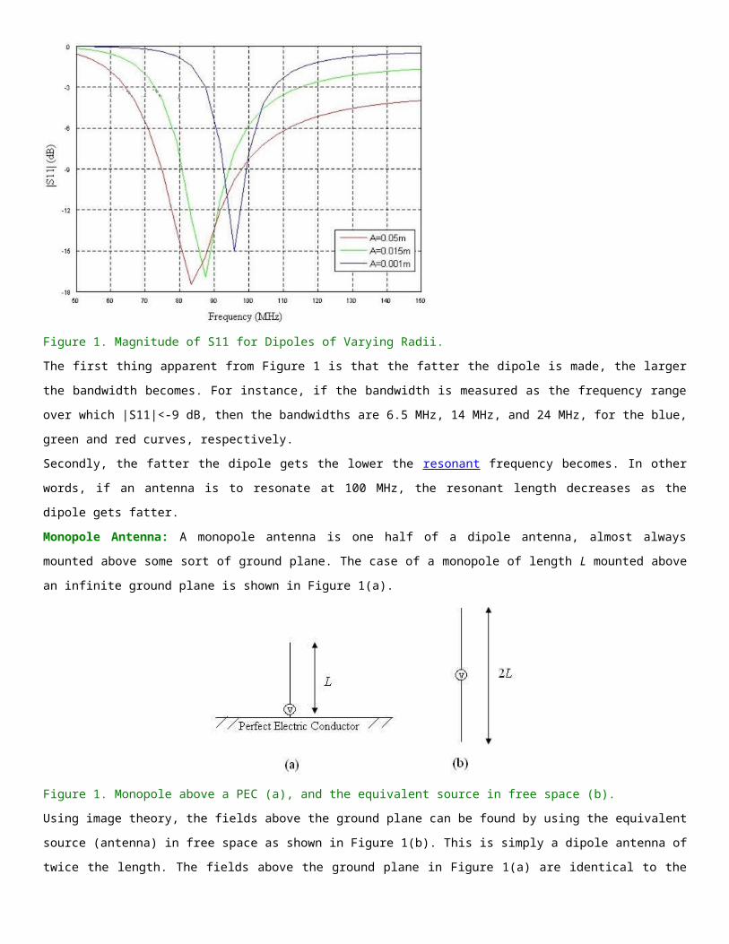
Figure 2. Normalized Radiation Pattern for Microstrip (Patch) Antenna.

The directivity of patch antennas is approximately 5-7 dB. The fields are linearly

polarized. Next we'll consider more aspects involved in Patch (Microstrip) antennas.

Consider a square patch antenna fed at the end as before. Assume the substrate is air (or styrofoam, with

a permittivity equal to 1), and that L=W=1.5 meters, so that the patch is to resonate at 100 MHz. The

height h is taken to be 3 cm. Note that microstrips are usually made for higher frequencies, so that they

are much smaller in practice. When matched to a 200 Ohm load, the magnitude of S11 is shown in Figure

1.

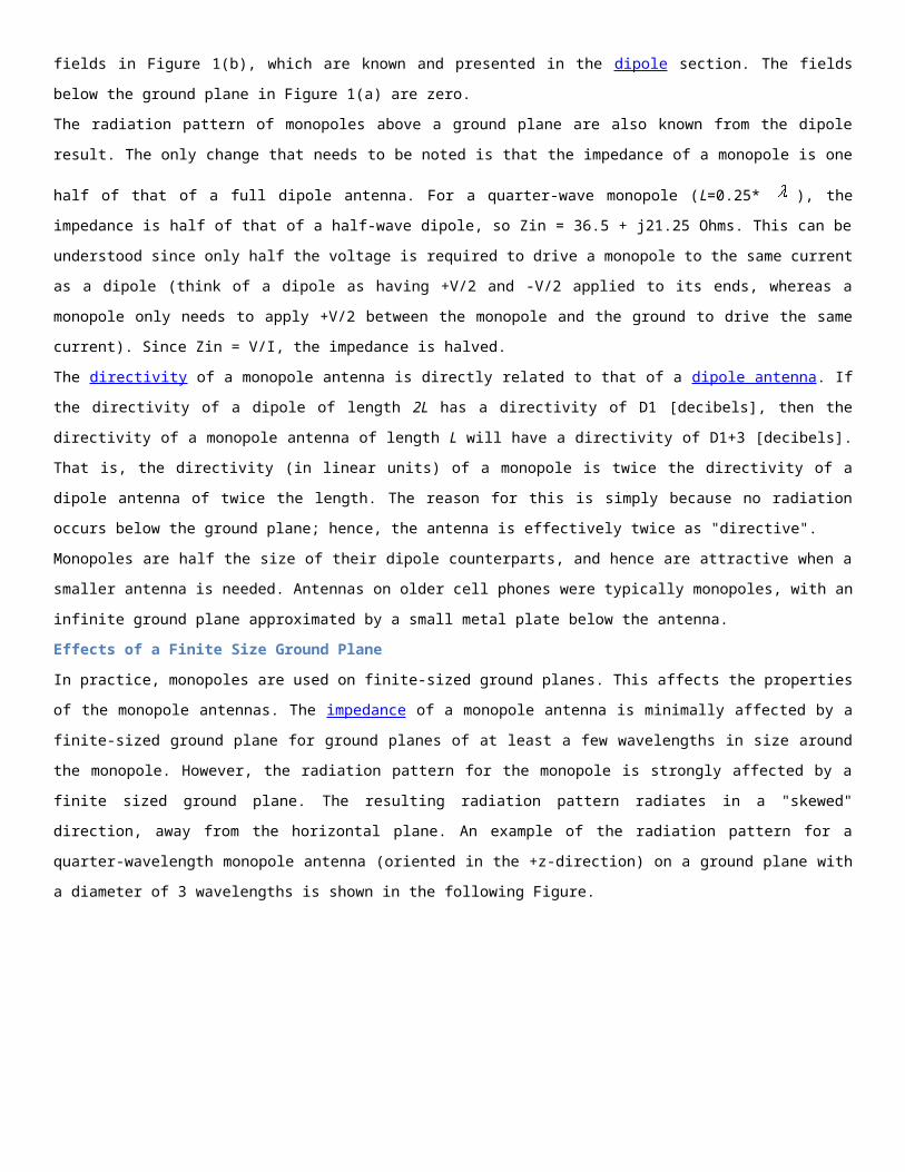
Figure 1. Magnitude of S11 versus Frequency.

Some noteworthy observations are apparent from Figure 1. First, the bandwidth of the patch antenna is

very small. Rectangular patch antennas are notoriously narrowband; the bandwidth of rectangular patches

are typically 3%. Secondly, the antenna was designed to operate at 100 MHz, but it is resonant at

approximately 96 MHz. This shift is due to fringing fields around the antenna, which makes the patch seem

longer. Hence, when designing a patch it is typically trimmed by 2-4% to achieve resonance at the desired

frequency.

The fringing fields around the antenna can help explain why the microstrip antenna radiates. Consider the

side view of a patch antenna, shown in Figure 2. Note that since the current at the end of the patch is zero

(open circuit end), the current is maximum at the center of the half-wave patch and (theoretically) zero at

the beginning of the patch. This low current value at the feed explains in part why the impedance is high

when fed at the end (we'll address this again later).

Since the patch antenna can be viewed as an open circuited transmission line, the voltage reflection

coefficient will be -1 (see the transmission line tutorial for more information). When this occurs, the voltage

and current are out of phase. Hence, at the end of the patch the voltage is at a maximum (say +V volts).

At the start of the patch (a half-wavelength away), the voltage must be at minimum (-V Volts). Hence, the

fields underneath the patch will resemble that of Figure 2, which roughly displays the fringing of the fields

around the edges.

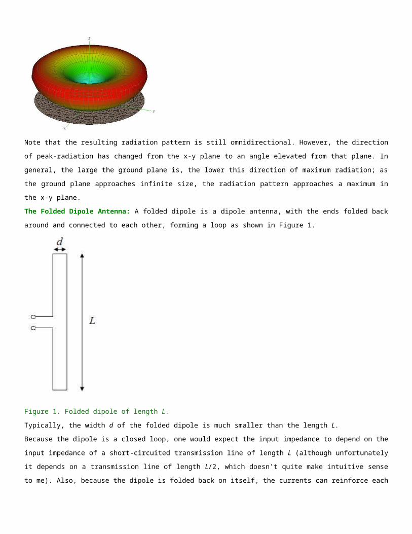
Figure 2. Side view of patch antenna with E-fields shown underneath.

It is the fringing fields that are responsible for the radiation. Note that the fringing fields near the surface

of the patch are both in the +y direction. Hence, these E-fields add up in phase and produce the radiation

of the microstrip antenna. As a side note, the smaller is, the more "bowed" the fringing fields become;

they extend farther away from the patch. Therefore, using a smaller permittivity for the substrate yields

better radiation. In contrast, when making a microstrip transmission line (where no power is to be

radiated), a high value of is desired, so that the fields are more tightly contained (less fringing),

resulting in less radiation. This is one of the trade-offs in patch antenna design. There have been research

papers written were distinct dielectrics (different permittivities) are used under the patch and transmission

line sections, to circumvent this issue.

Next, we'll look at alternative methods of feeding the antenna (connecting the antenna to the receiver or

transmitter).

Microstrip Antenna - Feeding Methods

Previous Antennas List Antenna Theory .com

Geometry and Fields Bandwidth & Fringing Fields Design and Tradeoffs

Inset Feed

Previously, the patch antenna was fed at the end as shown here. Since this typically

yields a high input impedance, we would like to modify the feed. Since the current is low

at the ends of a half-wave patch and increases in magnitude toward the center, the

input impedance (Z=V/I) could be reduced if the patch was fed closer to the center. One

method of doing this is by using an inset feed (a distance R from the end) as shown in

Figure 1.

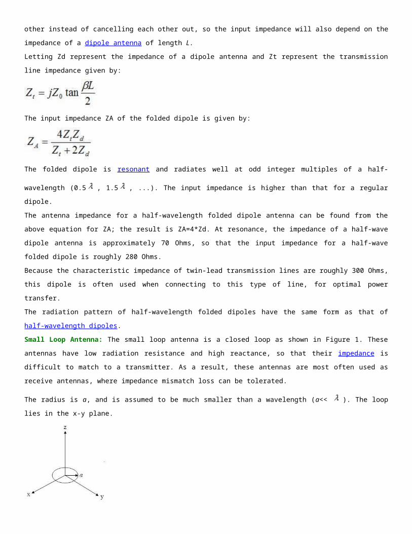
Figure 1. Patch Antenna with an Inset Feed.

Since the current has a sinusoidal distribution, moving in a distance R from the end will

increase the current by cos(pi*R/L) - this is just noting that the wavelength is 2*L, and so

the phase difference is 2*pi*R/(2*L) = pi*R/L.

The voltage also decreases in magnitude by the same amount that the current

increases. Hence, using Z=V/I, the input impedance scales as:

In the above equation, Zin(0) is the input impedance if the patch was fed at the end.

Hence, by feeding the patch antenna as shown, the input impedance can be decreased.

As an example, if R=L/4, then cos(pi*R/L) = cos(pi/4), so that [cos(pi/4)]^2 = 1/2. Hence,

a (1/8)-wavelength inset would decrease the input impedance by 50%. This method can

be used to tune the input impedance to the desired value.

Fed with a Quarter-Wavelength Transmission Line

The microstrip antenna can also be matched to a transmission line of characteristic

impedance Z0 by using a quarter-wavelength transmission line of characteristic

impedance Z1 as shown in Figure 2.

Figure 2. Patch antenna with a quarter-wavelength matching section.

The goal is to match the input impedance (Zin) to the transmission line (Z0). If the

impedance of the antenna is ZA, then the input impedance viewed from the beginning of

the quarter-wavelength line becomes

This input impedance Zin can be altered by selection of the Z1, so that Zin=Z0 and the

antenna is impedance matched. The parameter Z1 can be altered by changing the width

of the quarter-wavelength strip. The wider the strip is, the lower the characteristic

impedance (Z0) is for that section of line.

Coaxial Cable or Probe Feed

Microstrip antennas can also be fed from underneath via a probe as shown in Figure 3.

The outer conductor of the coaxial cable is connected to the ground plane, and the

center conductor is extended up to the patch antenna.

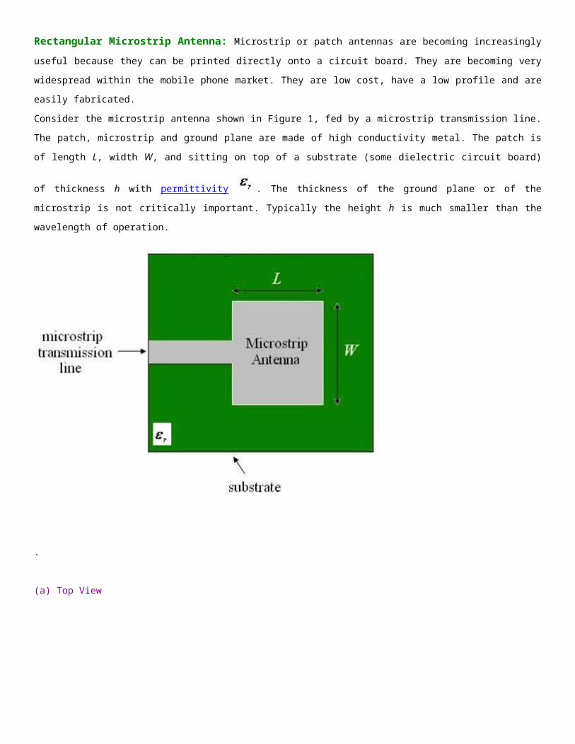
Figure 3. Coaxial cable feed of patch antenna.

The position of the feed can be altered as before (in the same way as the inset feed,

above) to control the input impedance.

The coaxial feed introduces an inductance into the feed that may need to be taken into

account if the height h gets large (an appreciable fraction of a wavelength). In addition,

the probe will also radiate, which can lead to radiation in undesirable directions.

Coupled (Indirect) Feeds

The feeds above can be altered such that they do not directly touch the antenna. For

instance, the probe feed in Figure 3 can be trimmed such that it does not extend all the

way up to the antenna. The inset feed can also be stopped just before the patch

antenna, as shown in Figure 4.

Figure 4. Coupled (indirect) inset feed.

The advantage of the coupled feed is that it adds an extra degree of freedom to the

design. The gap introduces a capacitance into the feed that can cancel out the

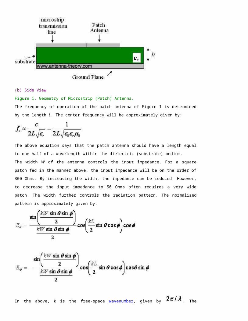
inductance added by the probe feed.

Aperture Feeds

Another method of feeding microstrip antennas is the aperture feed. In this technique,

the feed circuitry (transmission line) is shielded from the antenna by a conducting plane

with a hole (aperture) to transmit energy to the antenna, as shown in Figure 5.

Figure 5. Aperture coupled feed.

The upper substrate can be made with a lower permittivity to produce loosely bound

fringing fields, yielding better radiation. The lower substrate can be independently made

with a high value of permittivity for tightly coupled fields that don't produce spurious

radiation. The disadvantage of this method is increased difficulty in fabrication.

Microstrip Antenna - Design Parameters and Tradeoffs

Previous Antennas List Antenna Theory .com

Geometry & Radiated Fields Bandwidth & Fringing Fields Feeding Methods

All of the parameters in a rectangular patch antenna design (L, W, h, permittivity)

control the properties of the antenna. As such, this page gives a general idea of how the

parameters affect performance, in order to understand the design process.

First, the length of the patch L controls the resonant frequency as seen here. This is true

in general, even for more complicated microstrip antennas that weave around - the

length of the longest path on the microstrip controls the lowest frequency of operation.

Equation (1) below gives the relationship between the resonant frequency and the patch

length:

      (1)

Second, the width W controls the input impedance and the radiation pattern (see the

radiation equations here). The wider the patch becomes the lower the input impedance

is.

The permittivity of the substrate controls the fringing fields - lower permittivities

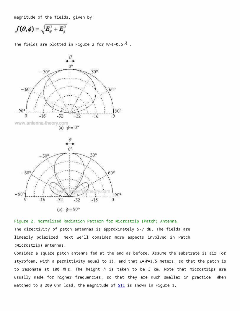
have wider fringes and therefore better radiation. Decreasing the permittivity also

increases the antenna's bandwidth. The efficiency is also increased with a lower value

for the permittivity. The impedance of the antenna increases with higher permittivities.

Higher values of permittivity allow a "shrinking" of the patch antenna. Particularly in cell

phones, the designers are given very little space and want the antenna to be a half-

wavelength long. One technique is to use a substrate with a very high permittivity.

Equation (1) above can be solved for L to illustrate this:

Hence, if the permittivity is increased by a factor of 4, the length required decreases by

a factor of 2. Using higher values for permittivity is frequently exploited in antenna

miniaturization.

The height of the substrate h also controls the bandwidth - increasing the height

increases the bandwidth. The fact that increasing the height of a patch antenna

increases its bandwidth can be understood by recalling the general rule that "an

antenna occupying more space in a spherical volume will have a wider bandwidth". This

is the same principle that applies when noting that increasing the thickness of a dipole

antenna increases its bandwidth. Increasing the height also increases the efficiency of

the antenna. Increasing the height does induce surface waves that travel within the

substrate (which is undesired radiation and may couple to other components).

The following equation roughly describes how the bandwidth scales with these

parameters:

Microstrip Antenna - Transient Fields (the Movie)

Previous Antennas List Antenna Theory .com

Geometry & Radiated Fields Bandwidth & Fringing Fields Feeding Methods

On this page, I will present a movie showing the fields under a microstrip antenna. In

this numerical experiment, a short pulse will be launched from the end of a microstrip,

which will travel towards the patch antenna. Some of the pulse will radiate away, and

some of the power will be reflected back down the microstrip line. This type of

simulation gives a little bit better idea of what is going on with a patch antenna,

specifically when short pulses (short waveforms, or brief applied voltages) are incident

upon a microstrip antenna.

Specifically, consider a patch antenna that is mounted on a ground plane, with a

dielectric with permittivity equal to 2.2. The thickness of this dielectric is 0.795 mm

(millimeters). The patch antenna will be 1.25 centimeters wide and 1.56 centimeters

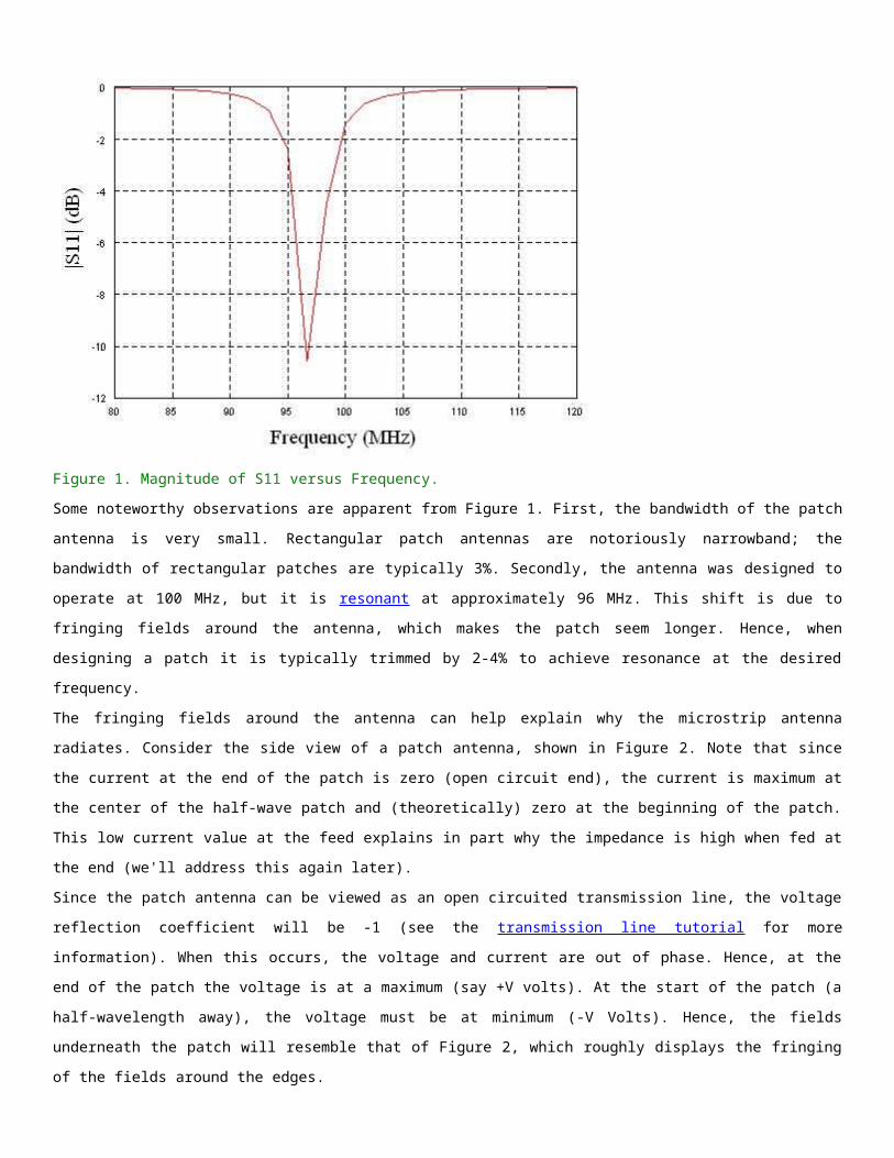
long (you should be able to tell what frequency this antenna will radiate well at - if not,

see intro to patch antennas page). The microstrip antenna will feed the patch offset from

the center, as shown in Figure 1.

Figure 1. Offset feed for Patch Antenna.

The transient pulse will be of the form given by exp(-(t-T0)/T )^2, where T0 is the time

delay and will be 45 pS (picoseconds, 10^-12), and T is a parameter that controls the

rate of rise and fall, which is 15 pS. This function is plotted in Figure 2.

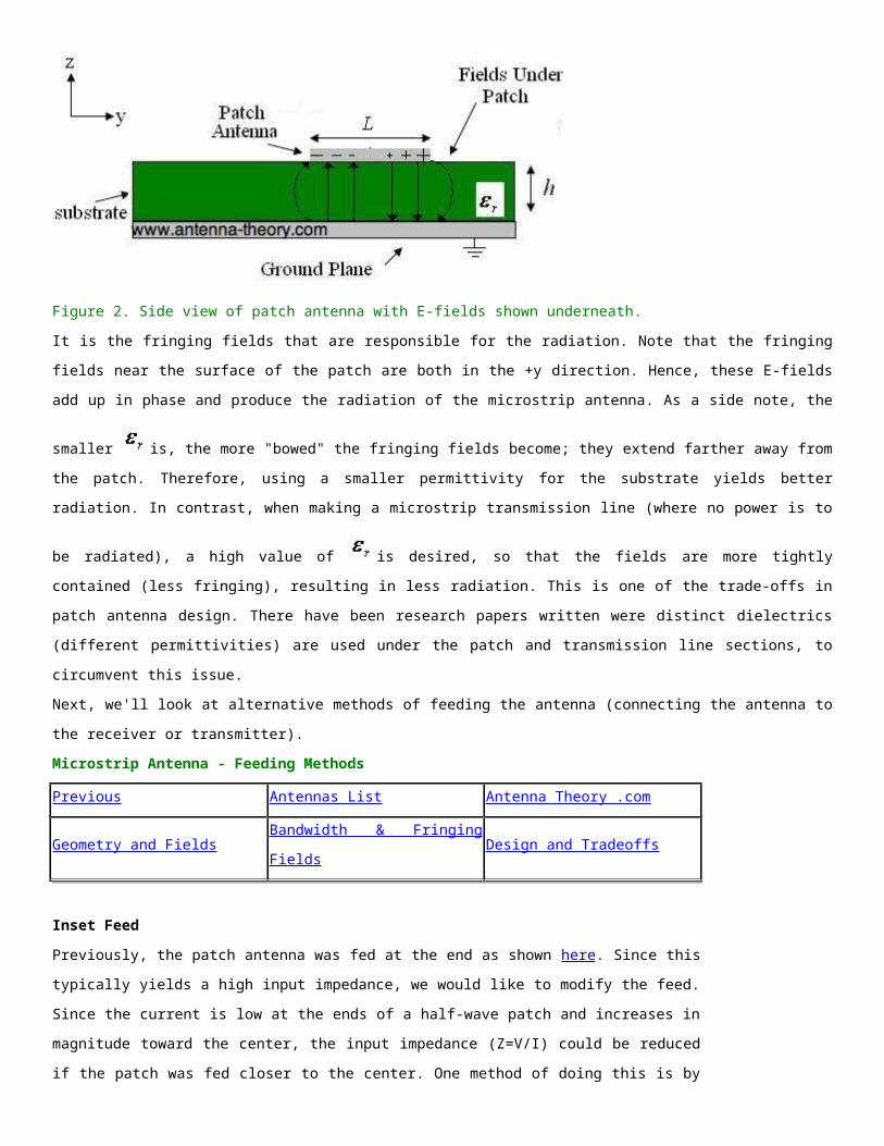
Figure 2. Incident (transient) pulse fed to a Patch Antenna.

In the following video, we will view the z-directed electric field, immediately below the

patch antenna. Note that the surface of the patch is normal to the z-axis. We can clearly

see the incident pulse propagate down the microstrip line, be disturbed by the microstrip

antenna, then some of the fields are reflected, some radiate away, and some stay

resonant below the patch and eventually radiate away or reflect back down the

microstrip line.

This video shows a Gaussian pulse travel down the microstrip. Some energy is reflected

back. Incidentally, taking the Fourier transform of the incident pulse and the returned

signal and taking the ratio would give S11 (return loss) as a function of frequency for this

antenna.

If you would like to see how this numerical electromagnetics simulation was developed,

see the patch antenna numerical example page.

Shorting Pins Used in Patch Antennas

Antennas List Antenna-Theory.com

Antenna designers are always looking for creative ways to improve performance. One

method used in patch antenna design is to introduce shorting pins (from the patch to the

ground plane) at various locations. To illustrate how this may help, two instances will be

illustrated.

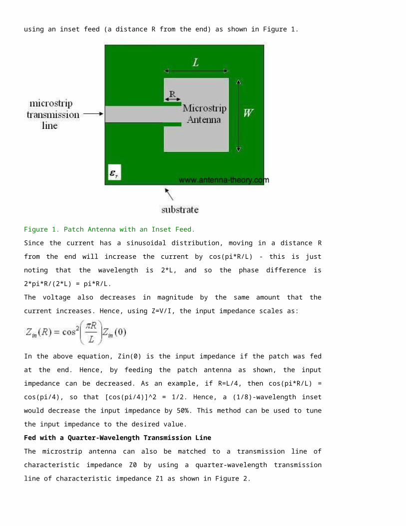
Quarter-Wavelength Patch

A quarter-wavelength patch shorted at the far end is shown Figure 1.

Figure 1. Quarter-wavelength patch with shorting pin at end.

Because the patch is shorted at the end, the current at the end of the patch is no longer

forced to be zero. As a result, this antenna actually has the same current-voltage

distribution as a half-wave patch antenna. However, the fringing fields which are

responsible for radiation are shorted on the far end, so only the fields nearest the

transmission line radiate. Consequently, the gain is reduced, but the patch antenna

maintains the same basic properties as a half-wavelength patch, but is reduced in size

50%.

Shorting Pin At the Feed to a Patch

A shorting pin can also be used at the feed to a patch antenna, as shown in Figure 2.

Figure 2. Half-wavelength patch with shorting pin at the feed.

You may be tempted to think that the shorting pin would zero out any power delivered

to the antenna. However, because patches are high frequency devices (typically used at

>1 GHz), the shorting pin actually introduces a parallel inductance to the antenna

impedance. The equivalent circuit of the above antenna is shown in Figure 3. The

antenna impedance is given by ZA, and the shorting pin introduces a reactance equal to

jX.

Figure 3. Equivalent Circuit of antenna in Figure 2.

The affect of the parallel inductance shifts the resonant frequency of the antenna. In

particular, the two components in parallel would result in their admittances (Y=1/Z)

adding. Hence, the admittance of the patch has a 1/(jX) added to it. In this manner, the

resonant frequency can be altered.

In addition, the shorting pin can become capacitive if instead of extending all the way to

the ground plane, it is left floating a small amount above. This introduces another design

parameter to optimize performance.

Planar Inverted F-Antenna (PIFA)

The PIFA antenna is increasingly used in the mobile phone market. This antenna

resembles an inverted F, which explains the name. It is popular because it has a low

profile and an omnidirectional pattern. The antenna is shown in Figure 4.

Figure 4. PIFA Antenna.

The PIFA is resonant at a quarter-wavelength, due to the shorting pin at the end. The

feed is placed between the open and shorted end, and the position controls the input

impedance.

The Corner Reflector Antenna

List of Antennas Home: Antenna Theory

To increase the directivity of an antenna, a fairly intuitive solution is to use a reflector.

For example, if we start with a wire antenna (lets say a half-wave dipole antenna), we

could place a conductive sheet behind it to direct radiation in the forward direction. To

further increase the directivity, a corner reflector may be used, as shown in Figure 1.

The angle between the plates will be 90 degrees.

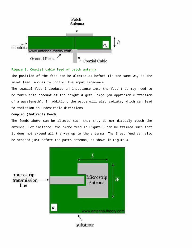
Figure 1. Geometry of Corner Reflector.

The radiation pattern of this antenna can be understood by using image theory, and

then calculating the result via array theory. For ease of analysis, we'll assume the

reflecting plates are infinite in extent. Figure 2 below shows the equivalent source

distribution, valid for the region in front of the plates.

Figure 2. Equivalent sources in free space.

The dotted circles indicate antennas that are in-phase with the actual antenna; the x'd

out antennas are 180 degrees out of phase to the actual antenna.

Assume that the original antenna has an omnidirectional pattern given by . Then

the radiation pattern (R) of the "equivalent set of radiators" of Figure 2 can be written

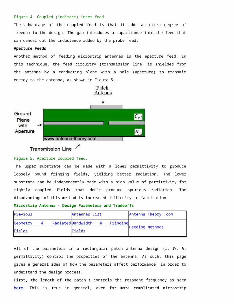
as:

The above directly follows from Figure 2 and array theory (k is the wave number. The

resulting pattern will have the same polarization as the original vertically polarized

antenna. The directivity will be increased by 9-12 dB. The above equation gives the

radiated fields in the region in front of the plates. Since we assumed the plates were

infinite, the fields behind the plates are zero.

The directivity will be the highest when d is a half-wavelength. Assuming the radiating

element of Figure 1 is a short dipole with a pattern given by , the fields for this

case are shown in Figure 3.

Figure 3. Polar and azimuth patterns of normalized radiation pattern.

The radiation pattern, impedance and gain of the antenna will be influenced by the

distance d of Figure 1. The input impedance is increased by the reflector when the

spacing is one half wavelength; it can be reduced by moving the antenna closer to the

reflector. The length L of the reflectors in Figure 1 are typically 2*d. However, if tracing a

ray travelling along the y-axis from the antenna, this will be reflected if the length is at

least . The height of the plates should be taller than the radiating element;

however since linear antennas do not radiate well along the z-axis, this parameter is not

critically important.

The Parabolic Reflector Antenna (Satellite Dish)

Antennas List Antenna Theory (Home)

Dishes: Basic Properties Gain Calculations and Efficiency Radiation Patterns

The most well-known reflector antenna is the parabolic reflector antenna, commonly known as a

satellite dish antenna. Examples of this dish antenna are shown in the following Figures.

Figure 1. The "big dish" of Stanford University.

Figure 2. A random "direcTV dish" on a roof.

Parabolic reflectors typically have a very high gain (30-40 dB is common) and low cross

polarization. They also have a reasonable bandwidth, with the fractional bandwidth being at

least 5% on commercially available models, and can be very wideband in the case of huge

dishes (like the Stanford "big dish" above, which can operate from 150 MHz to 1.5 GHz).

The smaller dish antennas typically operate somewhere between 2 and 28 GHz. The large

dishes can operate in the VHF region (30-300 MHz), but typically need to be extremely large at

this operating band.

The basic structure of a parabolic dish antenna is shown in Figure 3. It consists of a feed

antenna pointed towards a parabolic reflector. The feed antenna is often a horn antenna with a

circular aperture.

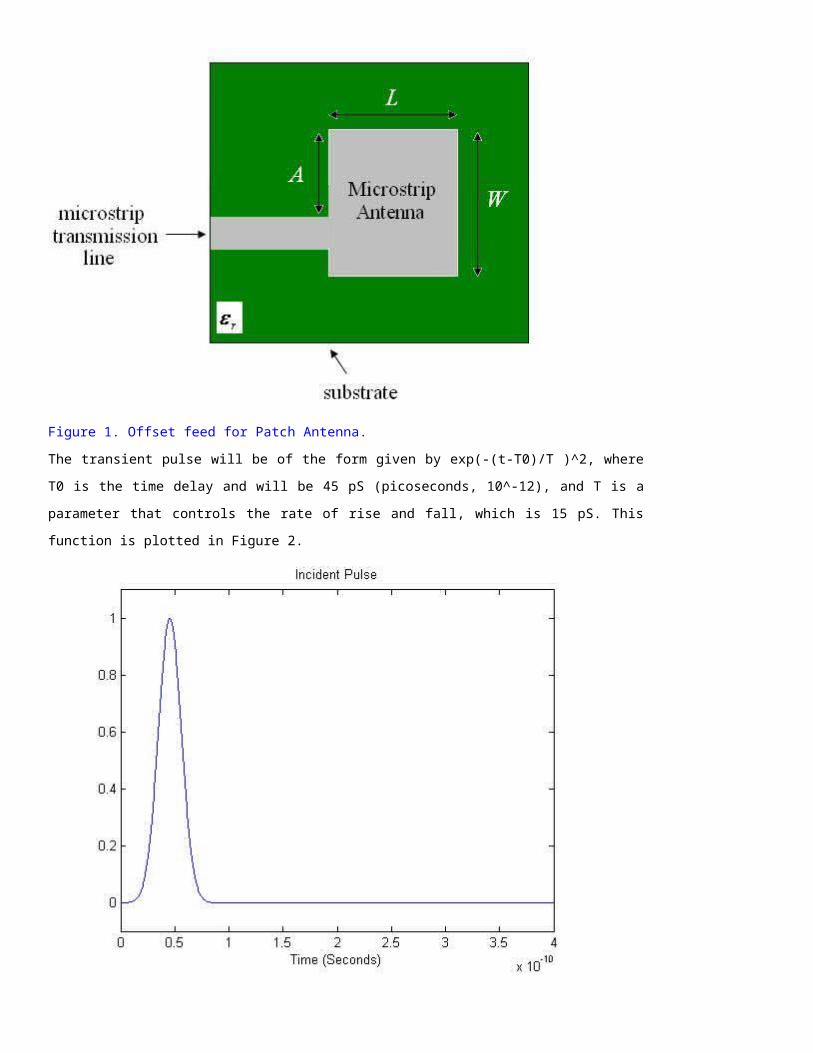
Figure 3. Components of a dish antenna.

Unlike resonant antennas like the dipole antenna which are typically approximately a half-

wavelength long at the frequency of operation, the reflecting dish must be much larger than a

wavelength in size. The dish is at least several wavelengths in diameter, but the diameter can

be on the order of 100 wavelengths for very high gain dishes (>50 dB gain). The distance

between the feed antenna and the reflector is typically several wavelenghts as well. This is in

contrast to the corner reflector, where the antenna is roughly a half-wavelength from the

reflector.

In the next section, we'll look at the parabolic dish geometry in detail and why a parabola is a

desired shape.

The Parabolic Reflector Antenna (Satellite Dish) 2

Previous: Parabolic Dishes (Page 1) Antennas List Antennas (Home)

On this page, we'll try to explain why a paraboloid makes a great reflector. To start, let the

equation of a parabola with focal length F can be written in the (x,z) plane as:

This is plotted in Figure 1.

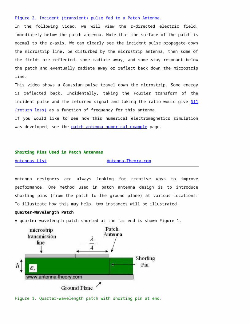
Figure 1. Illustration of parabola with defining parameters.

The parabola is completely described by two parameters, the diameter D and the focal length F.

We also define two auxilliary parameters, the vertical height of the reflector (H) and the max

angle between the focal point and the edge of the dish ( ). These parameters are related to

each other by the following equations:

To analyze the reflector, we will use approximations from geometric optics. Since the reflector is

large relative to a wavelength, this assumption is reasonable though not precisely accurate. We

will analyze the structure via straight line rays from the focal point, with each ray acting as a

plane wave. Consider two transmitted rays from the focal point, arriving from two distinct

angles as shown in Figure 2. The reflector is assumed to be perfectly conducting, so that the

rays are completely reflected.

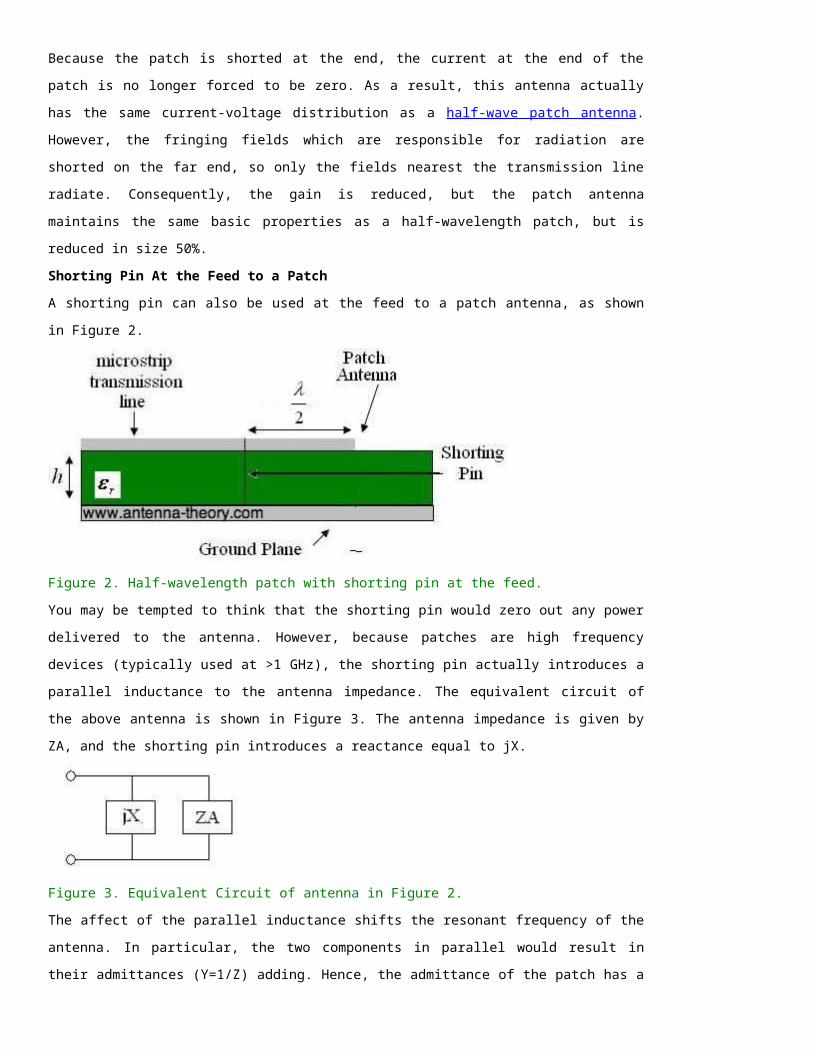
Figure 2. Two rays leaving the focal point and reflected from the parabolic reflector.

There are two observations that can be made from Figure 2. The first is that both rays end up

travelling in the downward direction (which can be determined because the incident and

reflected angles relative to the normal of the surface must be equal). . The rays are said to be

collimated. The second important observation is that the path lengths ADE and ABC are equal.

This can be proved with a little bit of geometry, which I won't reproduce here. These facts can

be proved for any set of angles chosen. Hence, it follows that:

All rays emanating from the focal point (the source or feed antenna) will be reflected towards

the same direction.

The distance each ray travels from the focal point to the reflector and then to the focal plane

is constant.

As a result of these observations, it follows the distribution of the field on the focal plane will be

in phase and travelling in the same direction. This gives rise to the parabolic dish antennas

highly directional radiation pattern. This is why the shape of the dish is parabolic.

Finally, by revolving the parabola about the z-axis, a paraboloid is obtained, as shown below.

For design, the value of the diameter D should be increased to increase the gain of the antenna.

The focal length F is then the only free parameter; typical values are commonly given as the

ratio F/D, which usually range between 0.3 and 1.0. Factors affecting the choice of this ratio will

be given in the following sections.

In the next section, we'll look at gain calculations for a parabolic reflector antenna.

The fields across the aperture of the parabolic reflector is responsible for this antenna's radiation. The

maximum possible gain of the antenna can be expressed in terms of the physical area of the aperture:

The actual gain is in terms of the effective aperture, which is related to the physical area by the efficiency

term ( ). This efficiency term will often be on the order of 0.6-0.7 for a well designed dish antenna:

Understanding this efficiency will also aid in understanding the trade-offs involved in the design of a

parabolic reflector. The efficiency can be written as the product of a series of terms:

We'll walk through each of these terms.

Radiation Efficiency

The radiation efficiency is the usual efficiency that deals with ohmic losses, as discussed on the

efficiency page. Since horn antennas are often used as feeds, and these have very little loss, and because

the parabolic reflector is typically metallic with a very high conductivity, this efficiency is typically close to

1 and can be neglected.

Aperture Taper Efficiency

The aperture radiation efficiency is a measure of how uniform the E-field is across the antenna's

aperture. In general, an antenna will have the maximum gain if the E-field is uniform in amplitude and

phase across the aperture (the far-field is roughly the Fourier Transform of the aperture fields). However,

the aperture fields will tend to diminish away from the main axis of the reflector, which leads to lower gain,

and this loss is captured within this parameter.

This efficiency can be improved by increasing the F/D ratio, which also lowers the cross-polarization of the

radiated fields. However, as with all things in engineering, there is a tradeoff: increasing the F/D ratio

reduces the spillover efficiency, discussed next.

Spillover Efficiency

The spillover efficiency is simple to understand. This measures the amount of radiation from the feed

antenna that is reflected by the reflector. Due to the finite size of the reflector, some of the radiation from

the feed antenna will travel away from the main axis at an angle greater than , thus not being reflected.

This efficiency can be improved by moving the feed closer to the reflector, or by increasing the size of the

reflector.

Other Efficiencies

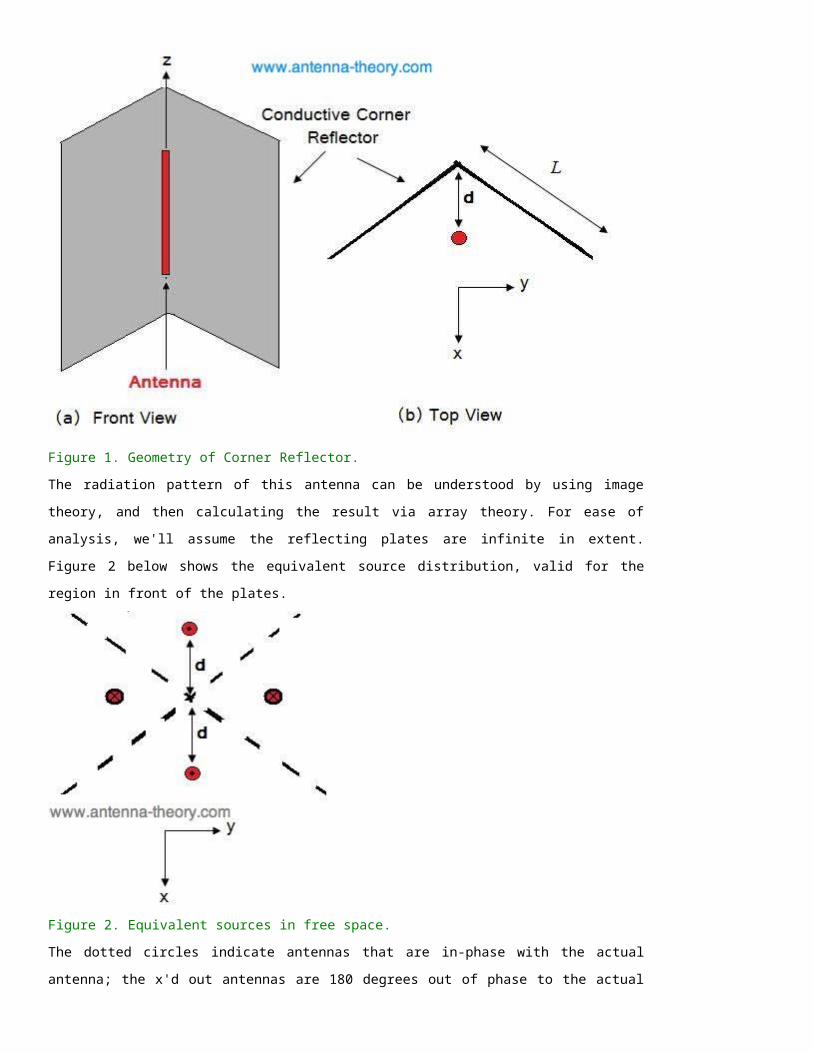
There are many other efficiencies that I've lumped into the parameter . This is a major of all other "real-

world effects" that degrades the antenna's gain and consists of effects such as:

Surface Error - small deviations in the shape of the reflector degrades performance, especially for high

frequencies that have a small wavelength and become scattered by small surface anomalies

Cross Polarization - The loss of gain due to cross-polarized (non-desirable) radiation

Aperture Blockage - The feed antenna (and the physical structure that holds it up) blocks some of the

radiation that would be transmitted by the reflector.

Non-Ideal Feed Phase Center - The parabolic dish has desirable properties relative to a single focal

point. Since the feed antenna will not be a point source, there will be some loss due to a non-perfect phase

center for a horn antenna.

Calculating Efficiency

The efficiency is a function of where the feed antenna is placed (in terms of F and D) and the feed

antenna's radiation pattern. Instead of introducing complex formulas for some of these terms, we'll make

use of some results by S. Silver back in 1949. He calculated the aperture efficiency for a class of radiation

patterns given as:

TYpically, the feed antenna (horn) will not have a pattern exactly like the above, but can be approximated

well using the function above for some value of n. Using the above pattern, the aperture efficiency of a

parabolic reflector can be calculated. This is displayed in Figure 1 for varying values of and the F/D

ratio.

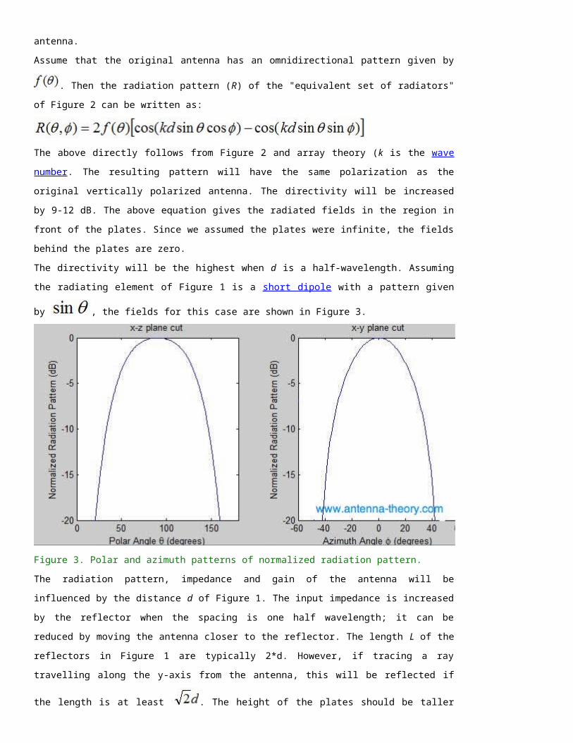
Figure 1. Aperture Efficiency of a Parabolic Reflector as a function of F/D or the angle , for varying feed

antenna radiation patterns.

Figure 1 gives a good idea on design of optimal parabolic reflectors. First, D is made as large as possible so

that the physical aperture is maximized. Then the F/D ratio that maximizes the aperture efficiency can be

found from the above graph. Note that the equation that relates the ratio of F/D to the angle can be

found here.

In the next section, we'll look at the radiation pattern of a parabolic antenna.

In this section, the 3d radiation patterns are presented to give an idea of what they look like. This example

will be for a parabolic dish reflector with the diameter of the dish D equal to 11 wavelengths. The F/D ratio

will be 0.5. A circular horn antenna will be used as the feed.

The maximum gain from the physical aperture is ; the actual gain is 29.3 dB = 851,

so we can conclude that the overall efficiency is 77%. The 3D patterns are shown in the following figures.

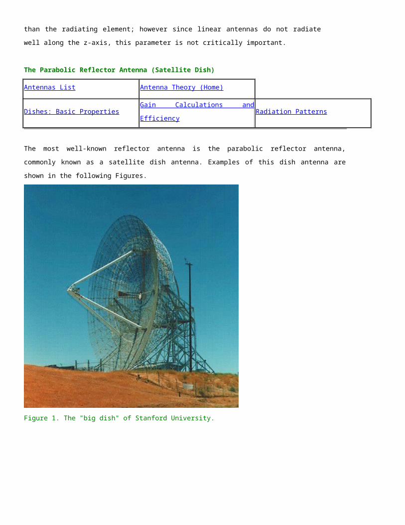
As can be seen, the pattern is highly directional. The HPBW is approximately 5 degrees, and the front-to-

back ratio is approximately 33 dB.

Helical Antenna

Antennas List Antenna Theory Home

Helix antennas have a very distinctive shape, as can be seen in the following picture.

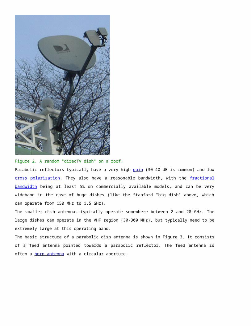
Photo courtesy of Dr. Lee Boyce.

The most popular helical antenna (often called a 'helix') is a travelling wave antenna in

the shape of a corkscrew that produces radiation along the axis of the helix. These

helixes are referred to as axial-mode helical antennas. The benefits of this antenna is it

has a wide bandwidth, is easily constructed, has a real input impedance, and can

produce circularly polarized fields. The basic geometry is shown in Figure 1.

Figure 1. Geometry of Helical Antenna.

The parameters are defined below.

D - Diameter of a turn on the helix.

C - Circumference of a turn on the helix (C=pi*D).

S - Vertical separation between turns.

- pitch angle, which controls how far the antenna grows in the z-direction per turn,

and is given by

N - Number of turns on the helix.

H - Total height of helix, H=NS.

The antenna in Figure 1 is a left handed helix, because if you curl your fingers on your

left hand around the helix your thumb would point up (also, the waves emitted from the

antenna are Left Hand Circularly Polarized). If the helix was wound the other way, it

would be a right handed helical antenna.

The pattern will be maximum in the +z direction (along the helical axis in Figure 1). The

design of helical antennas is primarily based on empirical results, and the fundamental

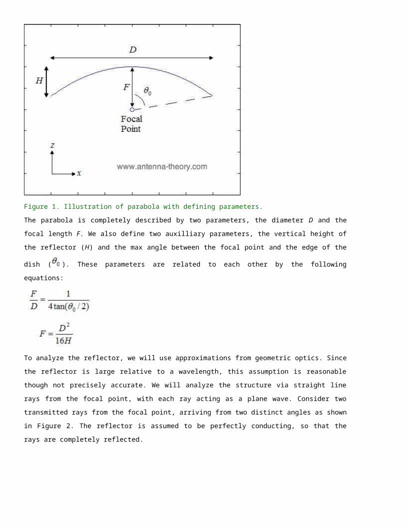
equations will be presented here.

Helices of at least 3 turns will have close to circular polarization in the +z direction when

the circumference C is close to a wavelength:

Once the circumference C is chosen, the inequalites above roughly determine the

operating bandwidth of the helix. For instance, if C=19.68 inches (0.5 meters), then the

highest frequency of operation will be given by the smallest wavelength that fits into the

above equation, or =0.75C=0.375 meters, which corresponds to a frequency of 800

MHz. The lowest frequency of operation will be given by the largest wavelength that fits

into the above equation, or =1.333C=0.667 meters, which corresponds to a

frequency of 450 MHz. Hence, the fractional BW is 56%, which is true of axial helices in

general.

The helix is a travelling wave antenna, which means the current travels along the

antenna and the phase varies continuously. In addition, the input impedance is primarly

real and can be approximated in Ohms by:

The helix functions well for pitch angles ( ) between 12 and 14 degrees. Typically, the

pitch angle is taken as 13 degrees.

The normalized radiation pattern for the E-field components are given by:

For circular polarization, the orthogonal components of the E-field must be 90 degrees

out of phase. This occurs in directions near the axis (z-axis in Figure 1) of the helix. The

axial ratio for helix antennas decreases as the number of loops N is added, and can be

approximated by:

The gain of the helix can be approximated by:

In the above, c is the speed of light. Note that for a given helix geometry (specified in

terms of C, S, N), the gain increases with frequency. For an N=10 turn helix, that has a

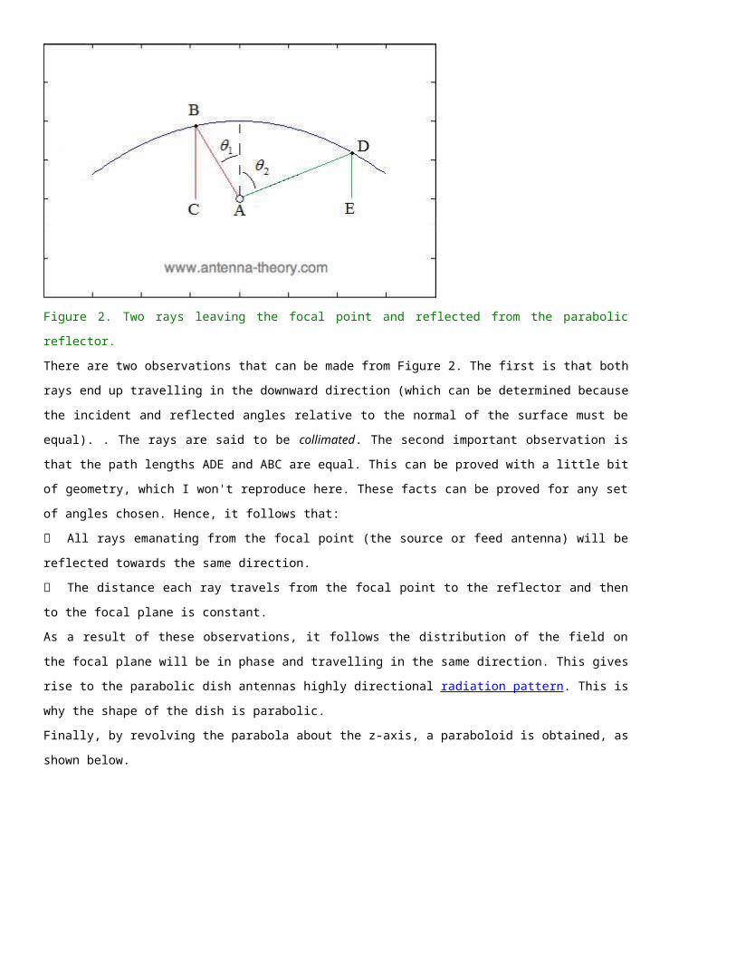
0.5 meter circumference as above, and an pitch angle of 13 degrees (giving S=0.13

meters), the gain is 8.3 (9.2 dB).

For the same example helix, the pattern is shown in Figure 2.

Figure 2. Normalized radiation pattern for helical antenna (dB).

The Half-Power Beamwidth for helical antennas can be approximated (in degrees) by:

Yagi-Uda Antenna

Antennas List Antenna Theory .com

The Yagi-Uda antenna or Yagi is one of the most brilliant antenna designs. It is simple

to construct and has a high gain, typically greater than 10 dB. These antennas typically

operate in the HF to UHF bands (about 3 MHz to 3 GHz), although their bandwidth is

typically small, on the order of a few percent of the center frequency. You are probably

familiar with this antenna, as they sit on top of roofs everywhere. An example of a Yagi-

Uda antenna is shown below.

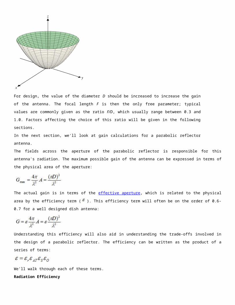
The Yagi antenna was invented in Japan, with results first published in 1926. The work

was originally done by Shintaro Uda, but published in Japanese. The work was presented

for the first time in English by Yagi (who was either Uda's professor or colleague, my

sources are conflicting), who went to America and gave the first English talks on the

antenna, which led to its widespread use. Hence, even though the antenna is often

called a Yagi antenna, Uda probably invented it. A picture of Professor Yagi with a Yagi-

Uda antenna is shown below.

In the next section, we'll explain the principles of the Yagi-Uda antenna.

The basic geometry of a Yagi-Uda antenna is shown in Figure 1.

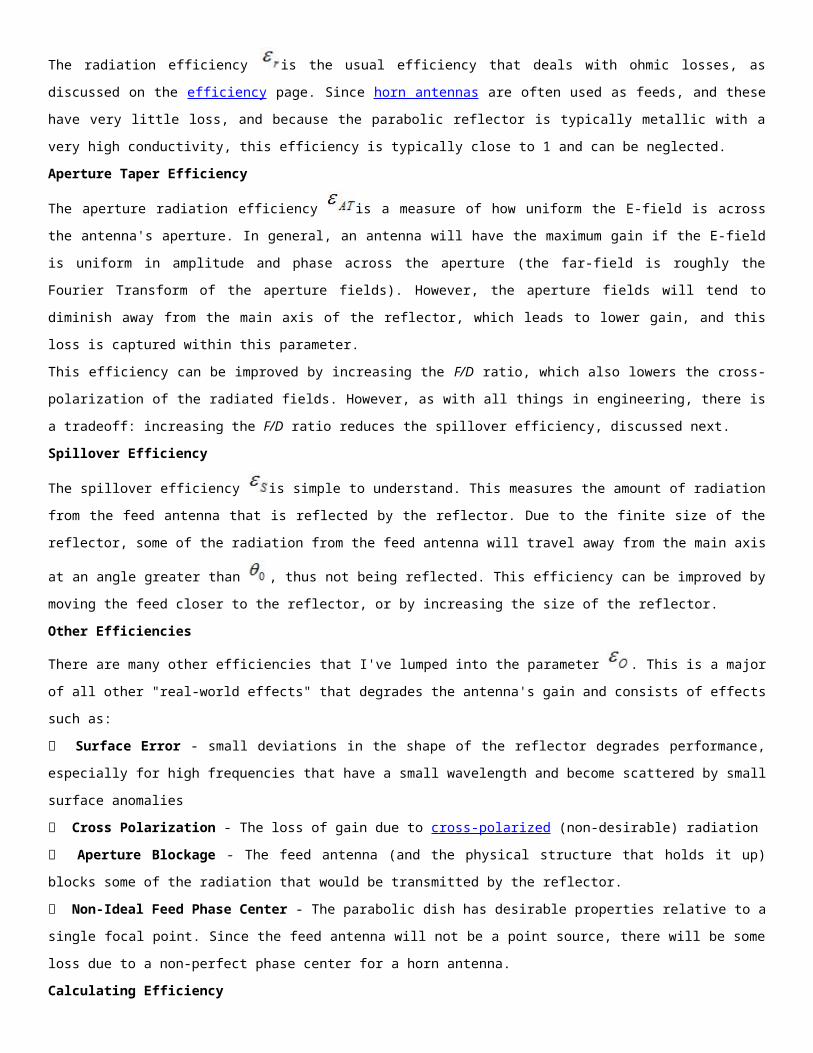
Figure 1. Geometry of Yagi-Uda antenna.

The antenna consists of a single 'feed' or 'driven' element, typically a dipole or a folded dipole antenna.

This is the only member of the above structure that is actually excited (a source voltage or current

applied). The rest of the elements are parasitic - they reflect or help to transmit the energy in a particular

direction. The length of the feed element is given in Figure 1 as F. The feed antenna is almost always the

second from the end, as shown in Figure 1. This feed antenna is often altered in size to make it resonant in

the presence of the parasitic elements (typically, 0.45-0.48 wavelengths long for a dipole antenna).

The element to the left of the feed element in Figure 1 is the reflector. The length of this element is given

as R and the distance between the feed and the reflector is SR. The reflector element is typically slightly

longer than the feed element. There is typically only one reflector; adding more reflectors improves

performance very slightly. This element is important in determining the front-to-back ratio of the antenna.

Having the reflector slightly longer than resonant serves two purposes. The first is that the larger the

element is, the better of a physical reflector it becomes. Secondly, if the reflector is longer than its

resonant length, the impedance of the reflector will be inductive. Hence, the current on the reflector lags

the voltage induced on the reflector. The director elements (those to the right of the feed in Figure 1) will

be shorter than resonant, making them capacitive, so that the current leads the voltage. This will cause a

phase distribution to occur across the elements, simulating the phase progression of a plane wave across

the array of elements. This leads to the array being designated as a travelling wave antenna. By choosing

the lengths in this manner, the Yagi-Uda antenna becomes an end-fire array - the radiation is along the

+y-axis as shown in Figure 1.

The rest of the elements (those to the right of the feed antenna as shown in Figure 1) are known as

director elements. There can be any number of directors N, which is typically anywhere from N=1 to N=20

directors. Each element is of length Di, and separated from the adjacent director by a length SDi. As

alluded to in the previous paragraph, the lengths of the directors are typically less than the resonant

length, which encourages wave propagation in the direction of the directors.

The above description is the basic idea of what is going on. Yagi antenna design is done most often via

measurements, and sometimes computer simulations. For instance, lets look at a two-element Yagi

antenna (1 reflector, 1 feed element, 0 directors). The feed element is a half-wavelength dipole, shortened

to be resonant (gain = 2.15 dB). The gain as a function of the separation is shown in Figure 2.

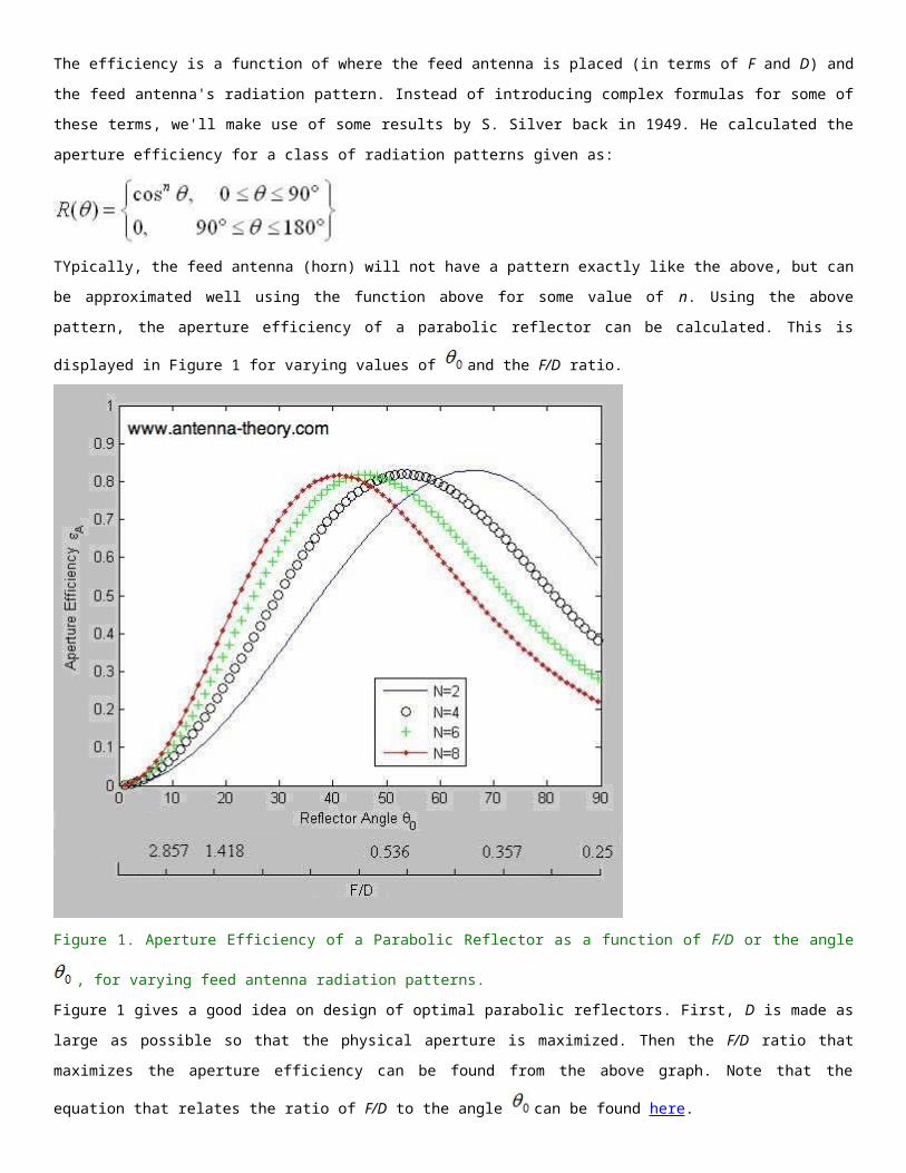
Figure 2. Gain versus separation for 2-element Yagi antenna.

The above graph shows that the gain is increases by about 2.5 dB if the separation SD is between 0.15 and

0.3 wavelengths. Similarly, the gain can be plotted as a function of director spacings, or as a function of

the number of directors used. Typically, the first director will add approximately 3 dB of overall gain (if

designed well), the second will add about 2 dB, the third about 1.5 dB. Adding an additional director

always increases the gain; however, the gain in directivity decreases as the number of elements gets

larger. For instance, if there are 8 directors, and another director is added, the increases in gain will be

less than 0.5 dB.

In the next section, I'll go further into the design of Yagi-Uda antennas.

The design of a Yagi-Uda antenna is actually quite simple. Because Yagi antennas have

been extensively analyzed and experimentally tested, the process basically follows this

outline:

Look up a table of design parameters for Yagi antennas

Build it (or model it numerically), and tweak it till the performance is acceptable

As an example, consider the table published in "Yagi Antenna Design" by P Viezbicke

from the National Bureau of Standards, 1968, given in Table I. Note that the "boom" is

the long element that the directors, reflectors and feed elements are physically attached

to, and dictates the lenght of the antenna.

Table I. Optimal Lengths for Yagi-Uda Elements, for Distinct Boom Lengths

d=0.0085

SR=0.2Boom Length of Yagi-Uda Array (in )

0.4 0.8 1.2 2.2 3.2 4.2

R 0.482 0.482 0.482 0.482 0.482 0.475

D1 0.442 0.428 0.428 0.432 0.428 0.424

D2 0.424 0.420 0.415 0.420 0.424

D3 0.428 0.420 0.407 0.407 0.420

D4 0.428 0.398 0.398 0.407

D5 0.390 0.394 0.403

D6 0.390 0.390 0.398

D7 0.390 0.386 0.394

D8 0.390 0.386 0.390

D9 0.398 0.386 0.390

D10 0.407 0.386 0.390

D11 0.386 0.390

D12 0.386 0.390

D13 0.386 0.390

D14 0.386

D15 0.386

Spacing

between

directors,

(SD/ )

0.20 0.20 0.25 0.20 0.20 0.308

Gain (dB) 9.25 11.35 12.35 14.40 15.55 16.35

There's no real rocket science going on in the above table. I believe the authors of the

above document did experimental measurements until they found an optimized set of

spacings and published it. The spacing between the directors is uniform and given in the

second-to-last row of the table. The diameter of the elements is given by d=0.0085 .

The above table gives a good starting point to estimate the required length of the

antenna (the boom length), and a set of lengths and spacings that achieves the

specified gain. In general, all the spacings, lengths, diamters (including the boom

diameter) are design variables and can be continuously optimized to alter performance.

There are thousands of tables that further give results, such as how the diamter of the

boom affects the results, and the optimal diamters of the elements.

As an example of Yagi-antenna radiation patterns, a 6-element Yagi antenna (with axis

along the +x-axis) is simulated in FEKO (1 reflector, 1 driven half-wavelength dipole, 4

directors). The resulting antenna has a 12.1 dBi gain, and the plots are given in Figures

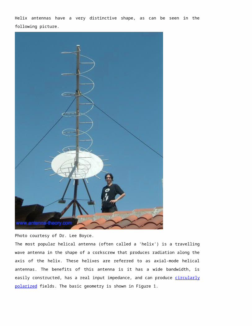
1-3.

Figure 1. E-plane gain of Yagi antenna.

Figure 2. H-Plane gain of Yagi antenna.

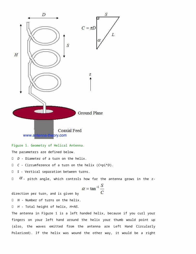
Figure 3. 3-D Radiation Pattern of Yagi antenna.

The above plots are just an example to give an idea of what the radiation pattern of the

Yagi-Uda antenna resembles. The gain can be increased (and the pattern made more

directional) by adding more directors or optimizing spacing (or rarely, adding another

refelctor). The front-to-back ratio is approximately 19 dB for this antenna, and this can

also be optimized if desired.

Slot Antennas

Antennas List Antenna Tutorial (Home)

Slot antennas are used typically at frequencies between 300 MHz and 24 GHz. These

antennas are popular because they can be cut out of whatever surface they are to be

mounted on, and have radiation patterns that are roughly omnidirectional (similar to a linear

wire antenna, as we'll see). The polarization is linear. The slot size, shape and what is behind

it (the cavity) offer design variables that can be used to tune performance.

Consider an infinite conducting sheet, with a rectangular slot cut out of dimensions a and b,

as shown in Figure 1. If we can excite some reasonable fields in the slot (often called the

aperture), we have an antenna.

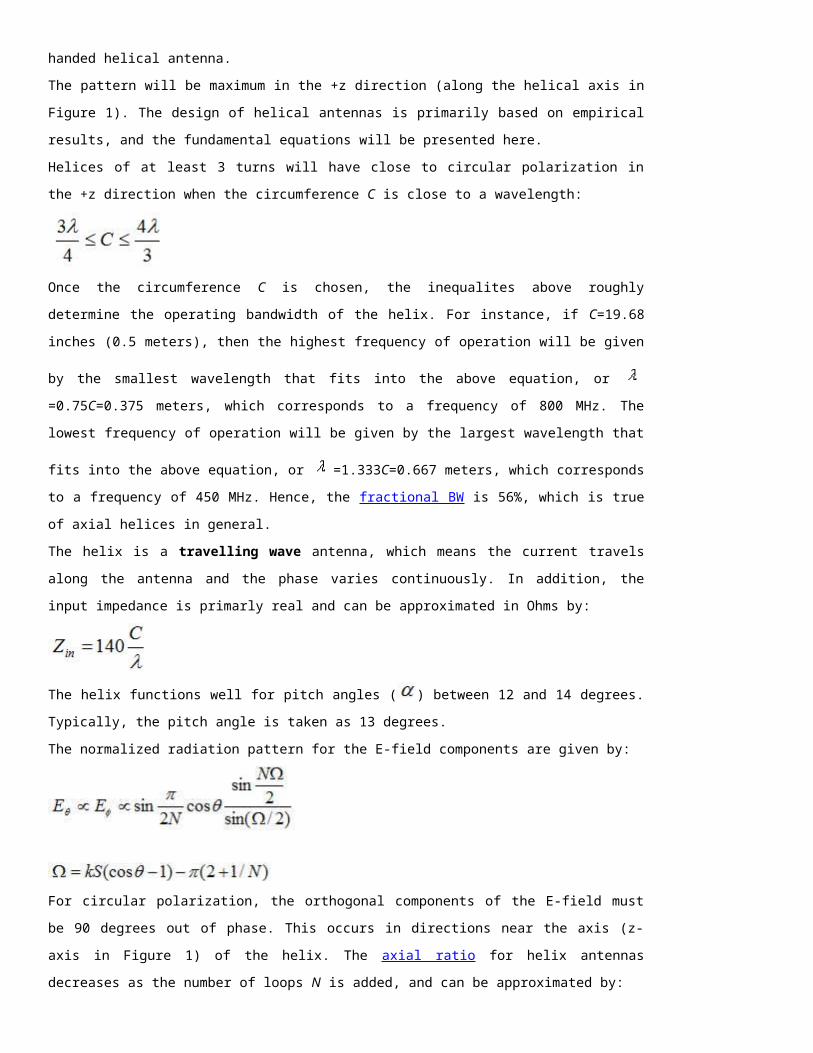
Figure 1. Rectangular Slot antenna with dimensions a and b.

To gain an intuition about slot antennas, first we'll learn Babinet's principle (put into antenna

terms by H. G. Booker in 1946). This principle relates the radiated fields and impedance of an

aperture or slot antenna to that of the field of its dual antenna. The dual of a slot antenna

would be if the conductive material and air were interchanged - that is, the slot antenna

became a metal slab in space. An example of dual antennas is shown in Figure 2:

Figure 2. Dual antennas.

Note that a voltage source is applied across the short end of the slot. This induces an E-field

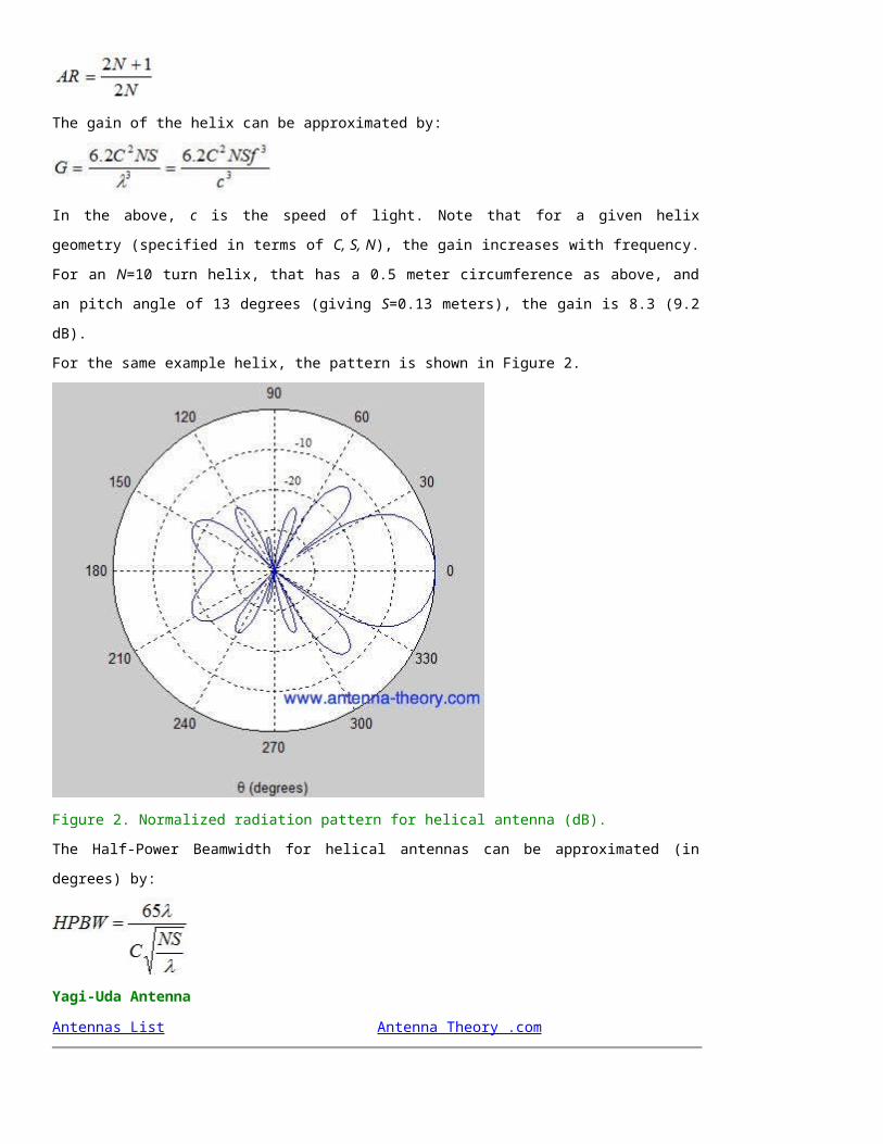
distribution within the slot, and currents that travel around the slot perimeter, both

contributed to radiation. The dual antenna is similar to a dipole antenna. The voltage source

is applied at the center of the dipole, so that the voltage source is rotated.

Babinet's principle relates these two antennas. The first result states that the impedance of

the slot ( ) is related to the impedance of its dual antenna ( ) by the relation:

In the above, is the intrinsic impedance of free space. The second major result of

Babinet's/Booker's principle is that the fields of the dual antenna are almost the same as the

slot antenna (the fields components are interchanged, and called "duals"). That is, the fields

of the slot antenna (given with a subscript S) are related to the fields of it's complement

(given with a subscript C) by:

Hence, if we know the fields from one antenna we know the fields of the other antenna.

Hence, since it is easy to visualize the fields from a dipole antenna, the fields and impedance

from a slot antenna can become intuitive if Babinet's principle is understood.

Note that the polarization of the two antennas are reversed. That is, since the dipole antenna

on the right in Figure 2 is vertically polarized, the slot antenna on the left will be horizontally

polarized.

Duality Example

As an example, consider a dipole similar to the one shown on the right in Figure 2. Suppose

the length of the dipole is 14.4 centimeters and the width is 2 centimeters, and that the

impedance at 1 GHz is 65+j15 Ohms. The fields from the dipole antenna are given by:

What are the fields from a slot at 1 GHz, with the same dimensions as the dipole?

Using Babinet's principle, the impedance can be easily found:

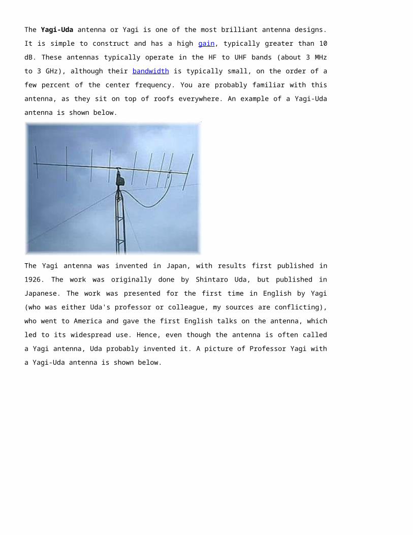
The impedance of the slot for this case is much larger, and while the dipole's impedance is

inductive (positive imaginary part), the slot's impedance is capacitive (negative imaginary

part). The E-fields for the slot can be easily found:

We see that the E-fields only contain a phi (azimuth) component; the antenna is therefore

horizontally polarized.

Cavity-Backed Slot Antennas

Previous: Slot Antennas Intro Antennas List Antenna Tutorial (Home)

The previous page introducing slot antennas was primarily theoretical (giving you an

intuitive idea of how slot antennas work); however, since it was about an infinite

conducting plane it is not entirely practical. A practical slot antenna is the cavity-

backed slot antenna. Unfortunately, the equations related to these antennas are

somewhat complicated and in my opinion don't give a good idea of how they work.

Hence, I'll present the basics, present some experimental results and try to give an idea

of design parameters.

The basic cavity-backed slot antenna is shown in Figure 1 (in a rectangular cube of size

A*B*C). The walls are metallic (electrically conducting), and the inside is hollow. On one

end, a slot is cut out. The cavity is typically excited by a probe antenna in the intererior

of the cavity, which typically is modelled as a monopole antenna. The exciting monopole

antenna is shown in green.

Figure 1. Cavity-backed slot antenna.

I'll give some experimental results for this antenna. Let the height of the cavity

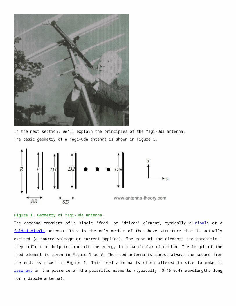
C=36mm, the length be A=87mm and the height B=36mm. The height of the monopole

antenna will be 29.5mm, so that the monopole is a quarter-wavelength long at 2.55 GHz.

The monopole will be centered about the cavity in the y-direction, and 61.5mm behind

the slot in the x-direction. The slot is 58mm long (in the y-direction) and 3 mm high (in

the z-direction).

S11 is measured for this antenna (relative to a 50 Ohm source), and is plotted versus

frequency in Figure 2.

Figure 2. S11 as a function of Frequency for Cavity-backed Slot.

The antenna has a first resonance at about 2.45 GHz. At this frequency, the slot antenna

is roughly 0.474 wavelengths long - which is roughly the length of a resonant dipole

antenna. S11 drops to below -20 dB at this frequency, indicating that most of the power

is radiated away. The bandwidth, measured (somewhat arbitrarily) as the frequency

span that S11 is less than -6 dB is roughly from 2.35 GHz to 2.55 GHz, giving a fractional

bandwidth of slightly over 8%.

Note that two other dips ('resonances') in the S11 curve occur, at approximately 3 GHz

and 4.18 GHz. At these frequencies, the slot length is 0.58 and 0.81 wavelengths,

respectively.

The volume of the cavity typically influences the bandwidth - a larger volume often

yields a higher bandwidth. The material within the cavity (so far I have assumed it was

filled with air), can be replaced with a dielectric medium. This reduces the resonant

length of slot, allowing for a smaller antenna. The tradeoff is that the bandwidth and

efficiency typically decrease with a dielectric cavity medium.

The radiation pattern at 2.45 GHz is now presented. The H-plane (xy plane) is shown on

the in Figure 3, and the E-plane (xz plane) is shown in Figure 4.

Figure 3. H-plane (xy plane). Angle measured off x-axis towards y-axis.

Figure 4. E-plane (xz plane). Angle measured off z-axis (to x-axis).

The radiation pattern somewhat resembles that of a dipole antena in the forward H-

plane. The 3-dB beamwidth is roughly 60 degrees in this plane. The radiation pattern is

diminished in the rear H-plane, with a significant back lobe about 6 dB down from the

peak of the main beam. In the E-plane, the pattern is fairly broad, with a 3-dB

beamwidht of about 120 degrees. The broad pattern of these antennas make them well

suited for use in antenna arrays. The peak gain of a thin slot is usually around 2-3 dB.

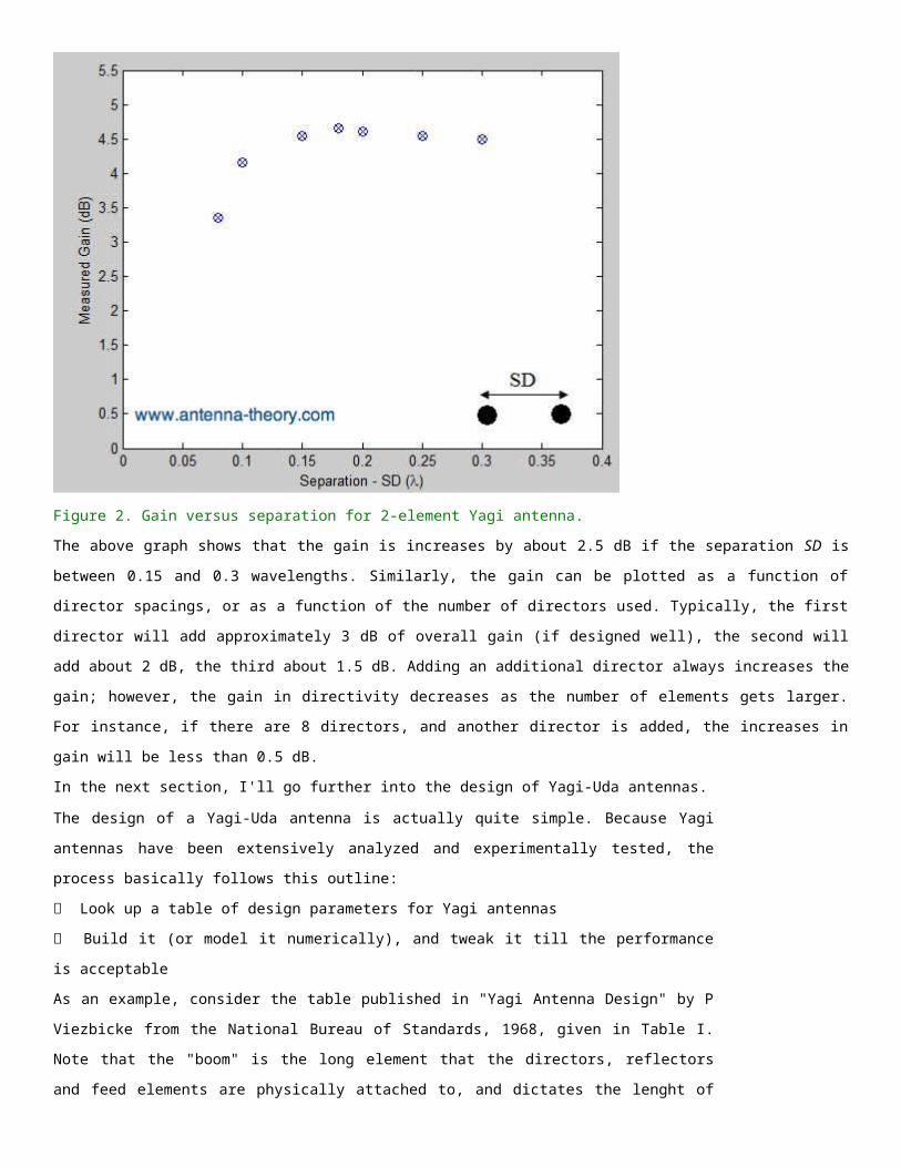
In the next section, we'll look at slotted waveguides.

Slotted Waveguide Antennas

Previous: Inverted F Antennas

(IFA)Antennas List Antenna Tutorial (Home)

Slotted antenna arrays used with waveguides are a popular antenna in navigation, radar

and other high-frequency systems. They are simple to fabricate, have low-loss (high

efficiency) and radiate linear polarization with low cross-polarization. These antennas are

often used in aircraft applications because they can be made to conform to the surface

on which they are mounted. The slots are typically thin (less than 0.1 of a wavelength)

and 0.5 wavelengths long (at the center frequency of operation).

The slots on the waveguide will assumed to have a narrow width. Increasing the width

increases the Bandwidth (recall that a fatter antenna often has an increased bandwidth);

the expense of a larger width is a higher degree of cross-polarization. The Fractional

Bandwidth for thin slots can be as low as 3-5%; wide slots can have a FBW on the order

of 75%. An example of a slotted waveguide array is shown in Figure 1 (dimensions given

by length a and width b)

Figure 1. Basic geometry of a slotted waveguide antenna.

As in the cavity-backed slot antenna, each slot could be independently fed with a

voltage source across the slot. However, (especially for large arrays) this would be very

difficult to construct, and I've never seen this done in practice. Instead, the waveguide is

used as the transmission line to feed the elements.

The position, shape and orientation of the slots will determine how (or if) they radiate. In

addition, the shape of the waveguide and frequency of operation will play a major role.

To understand what is going on, we'll need to understand the fields within the

waveguide first. For a primer on waveguides, see here: waveguide primer.

The dominant TE10 mode will be assumed to exist within the waveguide. Using the

geometry of Figure 1, the fields that exist within the waveguide are given by:

In the above, f is the frequency of interest, k is the wavenumber and is a constant

that specifies how much power is added to the waveguide.

Magnetic fields tangent to a conductor produce electric currents on the surface. The

resulting surface current density J [measured in Amps/meter] can be determined using

the unit normal to the surface (n) as:

On the top wall of the waveguide (where the slots are), the induced currents will be:

Radiation occurs when the currents must "go around" the slots in order to continue on

their desired direction. As an example, consider a narrow slot in the center of the

waveguide, as shown in Figure 2.

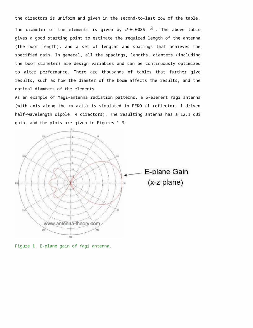
Figure 2. Waveguide with a thin slot centered about its width.

In this case, the z-component of the current will not be disturbed, because the slot is

thin and the z-current would not need to travel around the slot. Hence, the x-component

of the current will be responsible for the radiation. However, at this location (x=a/2), the

x-component of the current density is zero - i.e. no current and therefore no radiation. As

a result, slots can not be placed in the center of the waveguide as shown in Figure 2.

If the slots are displaced from the centerline as shown in Figure 1, the x-directed current

will not be zero and will need to travel around the slot. Hence, radiation will occur. Note

that the distance from the edge will determine the magnitude of the current. As a result,

the power that the slot radiates can be altered by moving the slots closer or farther from

the edge. In this manner, a phased array can be designed with varying excitation to

each element.

If the slot is oriented as shown in Figure 3, the slot will disturb the z-component of the

current density. This slot will then radiate. If this slot is displaced away from the center

line, the amount of power that it radiates can be adjusted.

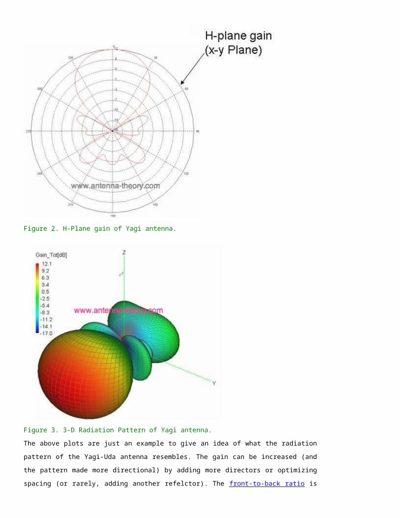
Figure 3. Horizontal slot in a waveguide.

If the slot is rotated at an angle about the centerline as shown in Figure 4, it will radiate.

The power it radiates will be a function of the angle (phi) that it is rotated - specifically

given by . Note that the z-component of the current is still responsible for

radiation in this case. The x-component is disturbed; however the currents will have

opposite magnitudes on either side of the centerline and will thus tend to cancel out the

radiation.

Figure 4. Rotated slot antenna in a waveguide.

In the next section, we'll examine slotted waveguides in more detail.

The most common slotted waveguide resembles that shown in Figure 1:

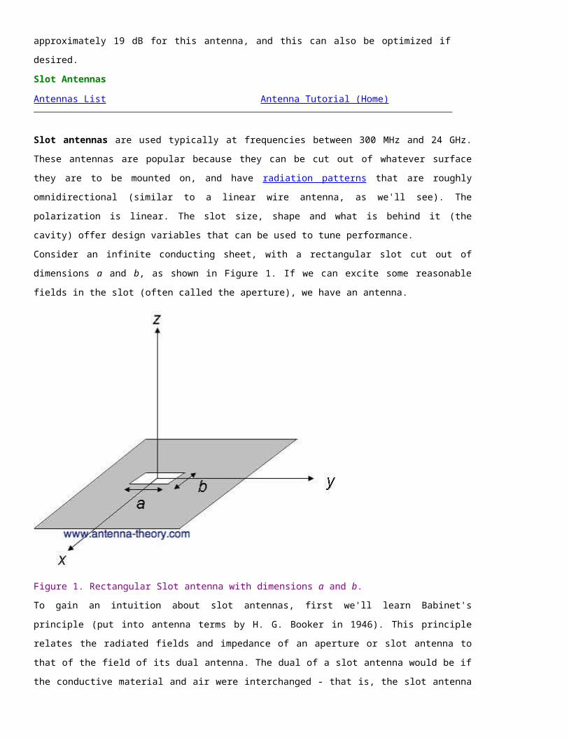
Figure 1. Geometry of the most common slotted waveguide antenna.

The front end (the open face at the y=0 in the x-z plane) is where the antenna is fed. The far end is usually

shorted (enclosed in metal). The waveguide may be excited by a short dipole (as seen on the cavity-

backed slot antenna) page, or by another waveguide.

To begin to analyze the antenna of Figure 1, lets view the circuit model. The waveguide itself acts as a

transmission line, and the slots in the waveguide can be viewed as parallel (shunt) admittances. The end

of the waveguide is short circuited, so a rough circuit model of Figure 1 is:

Figure 2. Circuit model of slotted waveguide antenna.

The last slot is a distance d from the end (which is short-circuited, as seen in Figure 2), and the slot

elements are spaced a distance L from each other.

Before we discuss choosing the sizes, they will be given in terms of the guide-wavelength, which is the

wavelength within the waveguide. The guide wavelength ( ) is a function of the width of the waveguide

(a) and the free space wavelength. For the dominant TE01 mode, the guide wavelength is given by:

The distance between the last slot and the end d is often chosen to be a quarter-wavelength. Transmission

line theory states that the impedance of a short circuit a quarter-wavelength down a transmission line is

an open circuit. Hence, Figure 2 then reduces to:

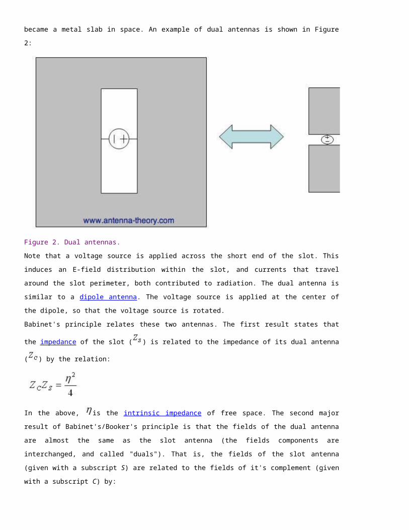
Figure 3. Circuit model of slotted waveguide using quarter-wavelength transformation.

If the parameter L is chosen to be a half-wavelength, then the input impedance of Z Ohms viewed a half-

wavelength away is Z Ohms. L is designed to be about a half-wavelength for this reason. If the waveguide

slot antenna is designed in this manner, then all of the slots can be viewed as being in parallel. Hence, the

input admittance and input impedance for an N element slotted array can be quickly calculated:

The input impedance of the waveguide is a function of the slot impedance.

Note that the above design parameters are only valid at a single frequency. As the frequency departs from

where the waveguide was designed to work, there will be degradation in the performance of the antenna.

To give an idea of the frequency characteristics of a slotted waveguide, a sample measurement of S11 as

a function of frequency will be shown. The waveguide is designed to operate at 10 GHz. It is fed by a

coaxial feed at the bottom as shown in Figure 4.

Figure 4. Slotted waveguide antenna fed by a coaxial feed.

The resulting S-parameter graph is shown in the following figure.

Note that the antenna has a very large drop in S11 around 10 GHz. This indicates that most of the power is

radiated away at this frequency. The bandwidth of the antenna (if defined as where S11 is less than -6 dB)

extends from about 9.7 GHz to 10.5 GHz, giving a Fractional Bandwidth of 8%. Note that there is also a

resonance at about 6.7 and 9.2 GHz. Below 6.5 GHz, the waveguide is below the cutoff frequency and

virtually no energy is radiated. The S-parameter graph shown above gives a good idea of what the

bandwidth and frequency characteristics of a slotted waveguide will resemble.

The 3D radiation pattern for the slotted waveguide is shown in the following figure (it was calculated using

a numerical electromagnetics package called FEKO). That gain is approximately 17 dB.

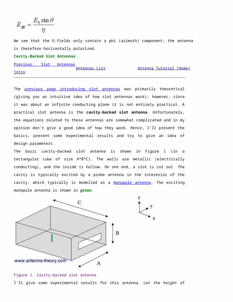
Note that in the x-z plane (or h-plane), the beamwidth is very narrow (2-5 degrees). In the y-z plane (or e-

plane), the beamwidth is much larger. Obtaining a more pencil-type beam using slotted waveguides is

discussed in the next section.

On the previous page on slotted waveguides, it was shown that for a single waveguide strip, the radiation

pattern tends to have a very wide beamwidth in the E-plane and a relatively small beamwidth in the H-

plane. The problem arises because the physical dimensions along the E-plane is much shorter than that

along the H-plane (the slotted waveguide is long but thin). In general, a longer antenna (or longer array)

produces a narrower beam.

This problem can be circumvented by arranging slotted waveguides in parallel, as shown in Figure 1.

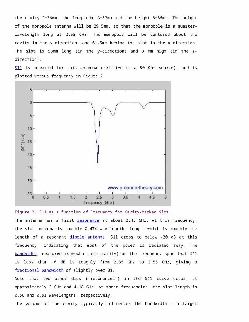
Figure 1. Array of slotted waveguides fed by a single source.

By stacking waveguides as shown in Figure 1, the E-plane beamwidth can be greatly reduced. In addition,

by adding a phase delay to each waveguide, the array of waveguides can be steered in the E-plane (see

phased arrays basics). The phase delay can be added by varying line lengths (then distinct frequencies will

produce distinct phase delays, allowing scanning simply by changing the frequency).

Antenna arrays made up of hundreds or even thousand elements are often slotted waveguides similar to

those described above. These are typically narrowband (a small deviation away from the design frequency

often change the impedance of the individual slots, and the many slots add up producing a highly reactive

impedance associated with the waveguide away from the resonant frequency). As an example, consider

Boeing's wedgetail:

While I don't know for certain, I would guess that the walls of the odd structure on top of the above

airplane contain a large slotted waveguide array, for scanning in the horizontal (azimuth) plane around the

airplane.

Power Handling capabilities of Slotted Waveguides

Slotted waveguides are often used because they are capable of transmitting high power levels. To give an

idea of what they are capable of (and introduce the practical constraint of power handling capabilities

versus altitude), I will present a brief table from Gilden and Gould's Handbook on High Power Capabilities

of Waveguide Systems.

The maximum power is shown in Table I. The max power is a function of the altitude, and will be further

divided as CW or "continuous wave" and a 1 microsecond pulse. The CW column gives the maximum

power handling capability of a slotted waveguide when the array is continuosly transmitting in MegaWatts

[MW]. The pulse column gives the maximum power when the waveguide radiates a brief pulse and then

shuts off. Note that the power handling capabilities of a waveguide decrease with altitude (given in feet).

The results are given for a typical X-band (10 GHz) waveguide; note that the power capabilities increases

as the frequency decreases and vice-versa.

Table I. Power versus altitude for a typical X-band (10 GHz) waveguide.

Altitude [ft] Max Power (CW) [MW] Max Power (1 uS Pulse) [MW]

0 0.95 1.05

10,000 0.55 0.62

20,000 0.25 0.30

30,000 0.15 0.20

40,000 0.06 0.10

50,000 0.03 0.05

Note that the power decreases rapidly with altitude; this is a necessary constraint to keep in mind in

designing radars for aircraft.

Inverted-F Antenna (IFA)

Previous: Cavity-Backed Slot

AntennasAntennas List Antenna Tutorial (Home)

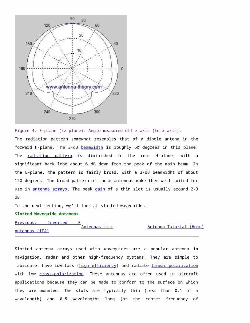
IFA Basics

The inverted-F antenna is shown in Figure 1. While this antenna appears to be a wire

antenna, after some analysis of how this antenna radiates, it is more accurately

classified as an aperture antenna.

Figure 1. Geometry of Inverted-F Antenna (IFA).

The feed is placed from the ground plane to the upper arm of the IFA. The upper arm of

the IFA has a length that is roughly a quarter of a wavelength. To the left of the feed (as

shown in Figure 1), the upper arm is shorted to the ground plane. The feed is closer to

the shorting pin than to the open end of the upper arm. The polarization of this antenna

is vertical, and the radiation pattern is roughly donut shaped, with the axis of the donut

in the vertical direction. The ground plane should be at least as wide as the IFA length

(L), and the ground plane should be at least lambda/4 in height. If the height of the

ground plane is smaller, the bandwidth and efficiency will decrease. The height of the

IFA (H), should be a small fraction of a wavelength. The radiation properties and

impedance are not a strong function of this parameter (H).

Because the structure somewhat resembles an inverted F, this antenna takes the name

"Inverted F Antenna".

Analysis

Why does this structure radiate? Lets go back and look at the slot antenna, shown in

Figure 2.

Figure 2. Geometry of Slot Antenna.

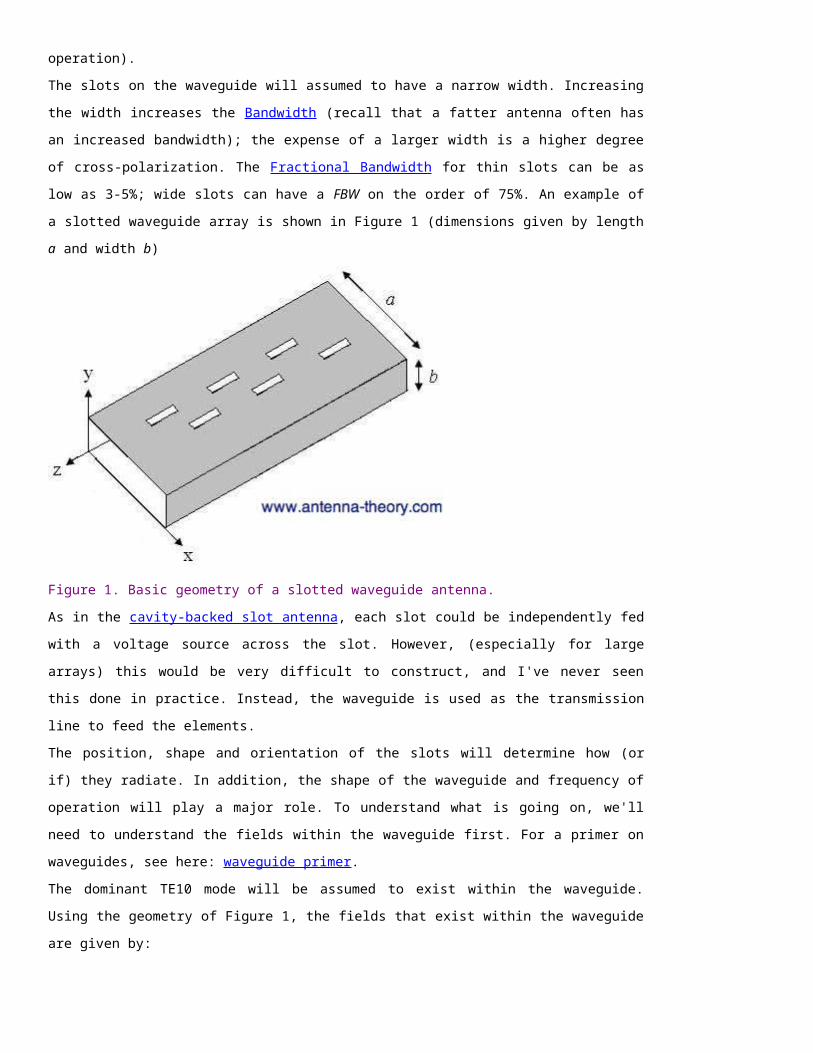
The slot antenna should be a half-wavelength long for proper radiation (more generally,

the perimeter of the slot antenna should be roughly one wavelength long). The way this

antenna is fed (or excited by the voltage source), the voltage at the ends of the slot

(across the aperture) must be zero because of the shorting posts on either side. If the

voltage is zero at the edges of the slot, then the voltage will be at a maximum a quarter-

wavelength away (at the center of the slot).

Now, where is the current at a maximum? Since this antenna can also be viewed as a

transmission line, the source basically "sees" a short circuited transmission line in either

direction. We know from transmission line theory that when a transmission line is short-

circuited, the voltage and current are 90 degrees out of phase. As a result, the current

will be zero at the center of the slot antenna, and will be maximum on the edges. The

voltage and current distributions are shown in Figure 3 (note the peak voltage is

assumed to be P volts, and the peak current is A Amps).

Figure 3. Voltage and Current Distribution along a Half-Wavelength Slot Antenna.

The slot antenna radiates because the voltage is in-phase across the entire aperture, so

that the E-field is vertical and lines up everywhere along the slot. This also gives rise to

the vertical polarization.

How does this relate to the IFA? Here is the key point: If the current at the center of the

slot is zero (as shown in Figure 3), then the slot antenna can be thought of as having an

open circuit at the center of the slot. Hence, if we break the slot in half, and get rid of

the right side, we are left with the IFA antenna as shown in Figure 1.

Note that the IFA can support the exact same mode of radiation. That is, since the IFA

has an open circuit on the right side of the feed (Figure 1), the current will be zero at

that point and the voltage will be a maximum - exactly as in the slot antenna case.

Hence, the IFA can be viewed as "half a slot antenna". And indeed, this is a valid model

for the antenna. Hence, the IFA is classified as an aperture antenna, even though the

aperture is not "closed".

Circuit Model for IFA (and Slot) Antennas

For effective radiation, we need the antenna to be a good radiating structure (the

currents or electric fields add up in phase), and we need to be able to get the energy

down the transmission line and onto the antenna. This means we need the impedance of

the antenna to be roughly 50 Ohms (typically). To accomplish this, it is desirable to have

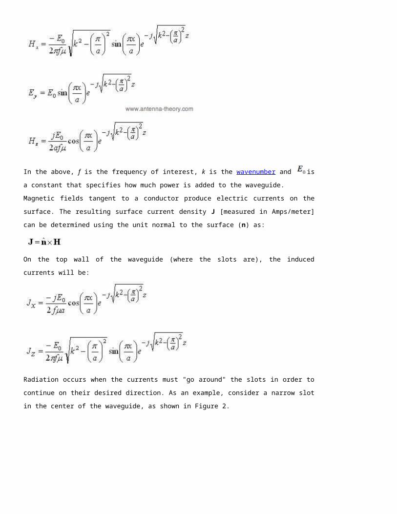
the reactive component of the impedance (imaginary part) to be zero. For the IFA or slot

antenna, note that the feed sees a shorted transmission line a small fraction of a

wavelength from the antenna. A shorted tx line that is a small fraction of a wavelength

creates an inductive reactive component. Similarly, the open circuit on the IFA creates a

capacitance to the right of the feed. The feed location is chosen to "balance out" the

capacitance (to the right of the feed) and the inductance (to the left of the feed as

shown in Figure 1). The inductance and capacitance cancel out, leaving just the radiation

resistance. An equivalent circuit model of the IFA is shown in Figure 4.

Figure 4. Circuit Model for IFA Antenna.

Note that for the slot antenna of Figure 2, the short-circuit to the right of the feed still

creates a capacitance, because the length of the slot to the right of the feed is larger

than a quarter-wavelength.

In regards to the real part of the impedance for an IFA or slot antenna, note that if the

slot antenna was fed at the center of the slot (where the voltage is maximum and the

current is zero --- Z=V/I), the impedance would be practically infinite, so that the

antenna would not radiate. By moving the feed away from the center for a slot, this also

allows the current to decrease from zero, which allows the impedance to drop to a more

desirable value. The same is true on the IFA antenna. Hence, the feed location is a

critical factor in designing an IFA or slot. A good location for the feed can easily be

obtained experimentally during an antenna design.

Examples of IFAs in the Real World

IFAs are commonly used in mobile phones due to their small size (quarter-wavelength).

An example of several IFAs in a mobile phone can be seen clearly on the Palm Pre. These

antennas are visible once the back cover is removed, shown in Figure 5:

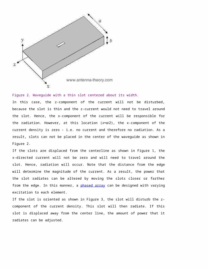
Figure 5. Palm Pre Antennas viewable by Removing Back Cover.

The yellow strip on the left side of the Palm Antenna is the GPS antenna, which is an IFA.

Since the GPS frequency is 1.575 GHz, a quarter wavelength is about 1.87 inches (4.75

cm). This is roughly the length of the IFA in the actual product (it is shortened for proper

tuning).

Two other antennas are visible in Figure 5. In the upper right side, there is the diversity

cell antenna, which. At the bottom of the device is a dual band IFA. This antenna is the

transmit/receive cell antenna, which should operate at the 900 MHz and 1800 MHz

bands. To do this, the antenna engineers made an IFA for the high band (1800 MHz),

which is the shorter arm shown in Figure 5. Using the same feed and shorting pin, they

branched off another arm for the low band (the longer arm, that is wrapped around itself

somewhat). Because the designers had limited space (which is a big challenge in mobile

phone antenna development), they wrapped the IFA around itself on the edges. By doing

this, they were able to obtain the required length for a 900 MHz IFA. However, by

wrapping the antenna around itself, the bandwidth and radiation efficiency decrease. In

summary, the IFA antenna is useful because of its small size and easy construction. In

the next section, we'll look at slotted waveguide antennas.

Horn Antenna - Intro

Antennas List Main Page

Next: More on Horns Horn Radiation Patterns

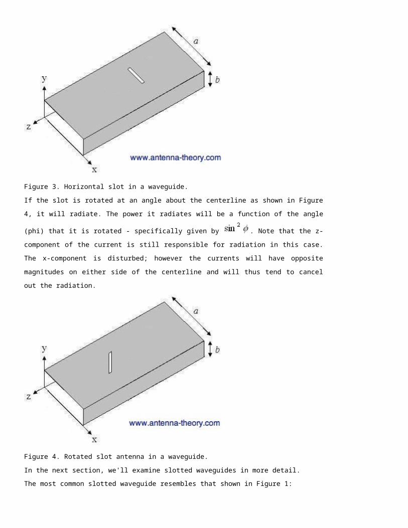
Horn antennas are very popular at UHF (300 MHz-3 GHz) and higher frequencies (I've

heard of horns operating as high as 140 GHz). They often have a directional radiation

pattern with a high gain , which can range up to 25 dB in some cases, with 10-20 dB

being typical. Horns have a wide impedance bandwidth, implying that the input

impedance is slowly varying over a wide frequency range (which also implies low values

for S11 or VSWR). The bandwidth for practical horn antennas can be on the order of 20:1

(for instance, operating from 1 GHz-20 GHz), with a 10:1 bandwidth not being

uncommon.

The gain often increases (and the beamwidth decreases) as the frequency of operation

is increased. Horns have very little loss, so the directivity of a horn is roughly equal to its

gain.

Horn antennas are somewhat intuitive and not relatively simple to manufacture. In

addition, acoustic horns also used in transmitting sound waves (for example, with a

megaphone). Horn antennas are also often used to feed a dish antenna, or as a

"standard gain" antenna in measurements.

Popular versions of the horn antenna include the E-plane horn, shown in Figure 1. This

horn is flared in the E-plane, giving the name. The horizontal dimension is constant at w.

Figure 1. E-plane horn.

Another example of a horn is the H-plane horn, shown in Figure 2. This horn is flared in

the H-plane, with a constant height for the waveguide and horn of h.

Figure 2. H-Plane horn.

The most popular horn is flared in both planes as shown in Figure 3. This is a pyramidal

horn, and has width B and height A at the end of the horn.

Figure 3. Pyramidal horn.

Horns are typically fed by a section of a waveguide, as shown in Figure 4. The

waveguide itself is often fed with a short dipole, which is shown in red in Figure 4. A

waveguide is simply a hollow, metal cavity. Waveguides are used to guide

electromagnetic energy from one place to another. The waveguide in Figure 4 is a

rectangular waveguide of width b and height a, with b>a. The E-field distribution for the

dominant mode is shown in the lower part of Figure 1.

Figure 4. Waveguide used as a feed to horn antennas.

Antenna texts typically derive very complicated functions for the radiation pattern. To do this, first the E-

field across the aperture of the horn is assumed, and the far-field radiation pattern is calculated using the

radiation equations. While this is conceptually straight forward, the resulting field functions end up being

extremely complex, and personally I don't feel add a whole lot of value. If you would like to see these

derivations, pick up any antenna textbook that has a section on horn antennas. (Also, as a practicing

antenna engineer, I can assure you that we never use radiation integrals to estimate patterns. We always

go on previous experience, computer simulations and measurements.)

Instead of the traditional academic derivation approach, I'll state some results for the horn and show some

typical radiation patterns, and attempt to provide a feel for the design parameters of horn antennas. Since

the pyramidal horn is the most popular, we'll analyze that. The E-field distribution across the aperture of

the horn is what is responsible for the radiation.

The radiation pattern of a horn will depend on B and A (the dimensions of the horn at the opening) and R

(the length of the horn, which also affects the flare angles of the horn), along with b and a (the dimensions

of the waveguide). These parameters are optimized in order to taylor the performance of the antenna, and

are illustrated in the following Figures.

Figure 1. Cross section of waveguide, cut in the H-plane.

Figure 2. Cross section of waveguide, cut in the E-plane.

Observe that the flare angles ( and ) depend on the height, width and length of the horn.

Given the coordinate system of Figure 2 (which is centered at the opening of the horn), the radiation will

be maximum in the +z-direction (out of the screen).

Figure 2. Coordinate system used, centered on the horn opening.

The E-field distribution across the opening of the horn can be approximated by:

The E-field in the far-field will be linearly polarized, and the magnitude will be given by:

The above equation states that the far-fields of the horn antenna are the Fourier Transform of the fields at

the opening of the horn. Many textbooks evaluate this integral, and end up with supremely complicated

functions, that I don't feel sheds a whole lot of light on the patterns.

Horn Antenna - Radiation Patterns

Antennas List Home: Antenna Theory

Horn Intro Previous: Horns 2

To give an idea of the fields from a horn, a specific example will be given. The

waveguide dimensions are given by a=3.69 inches, b=1.64 inches,

inches, A=30 inches, and B=23.8 inches. This horn is somewhat large, and will work well

above roughly 2 GHz. Horns made for higher frequencies are smaller. This horn antenna,

with a waveguide feed is shown in Figure 1.

Figure 1. Horn antenna described above.

This antenna is simulated using a commercial solver, FEKO (which runs method of

moments). The radiation pattern at 2 GHz is shown in Figure 2.

Figure 2. Horn radiation pattern at 2 GHz.

The gain of the horn is 18.1 dB in the +z-direction. The half-power beamwidth is 15

degrees in the xz-plane (H-plane) and 11 degrees in the yz-plane (E-plane).

The gain at 1.5 GHz is -2.54 dB, approximately 20 dB lower than at 2 GHz. The

waveguide feed acts as a high-pass filter; it blocks energy below its 'cutoff' frequency

and passes energy above this level. At 2.5 GHz, the gain increases slightly to 18.8 dB.

The horn geometry affects the gain of the antenna. For a desired gain, there are tables

and graphs that can be consulted in antenna handbooks that describe the optimal

geometry in terms of the length and aperture size of the horn. However, this optimal

geometry is only valid at a single frequency. Since horns are to operate over a wide

frequency band, they are often designed to have optimal gain at the lowest frequency in

the band. At higher frequencies, the geometry is no longer optimal, so the E-field across

the aperture is not optimal. However, the horn's aperture becomes electrically larger at

higher frequencies (the aperture is more wavelengths long as the frequency increases or

the wavelength decreases). Consequently, the loss of an optimal aperture field is offset

by an electrically larger horn, and the gain actually increases as the frequency

increases.

Antenna Arrays

Back: Antenna Theory

An antenna array (often called a 'phased array') is a set of 2 or more antennas. The

signals from the antennas are combined or processed in order to achieve improved

performance over that of a single antenna. The antenna array can be used to:

increase the overall gain

provide diversity reception

cancel out interference from a particular set of directions

"steer" the array so that it is most sensitive in a particular direction

determine the direction of arrival of the incoming signals

to maximize the Signal to Interference Plus Noise Ratio (SINR)

To understand antenna arrays, navigate through the following pages:

Basic Concepts and Intro to Antenna Arrays

Weighting Methods Used in Antenna Arrays

Geometry Optimization in Antenna Arrays

Introduction to Antenna Arrays

Arrays Main Page Antenna - Theory

Next: Intro to Arrays Page 2 The Array Factor

An antenna array is a set of N spatially separated antennas. The number of antennas in

an array can be as small as 2, or as large as several thousand (as in the AN/FPS-85

Phased Array Radar Facility operated by U. S. Air Force). In general, the performance of

an antenna array (for whatever application it is being used) increases with the number

of antennas (elements) in the array; the drawback of course is the increased cost, size,

and complexity.

The following figures show some examples of antenna arrays.

Figure 1. Four-element microstrip antenna array.

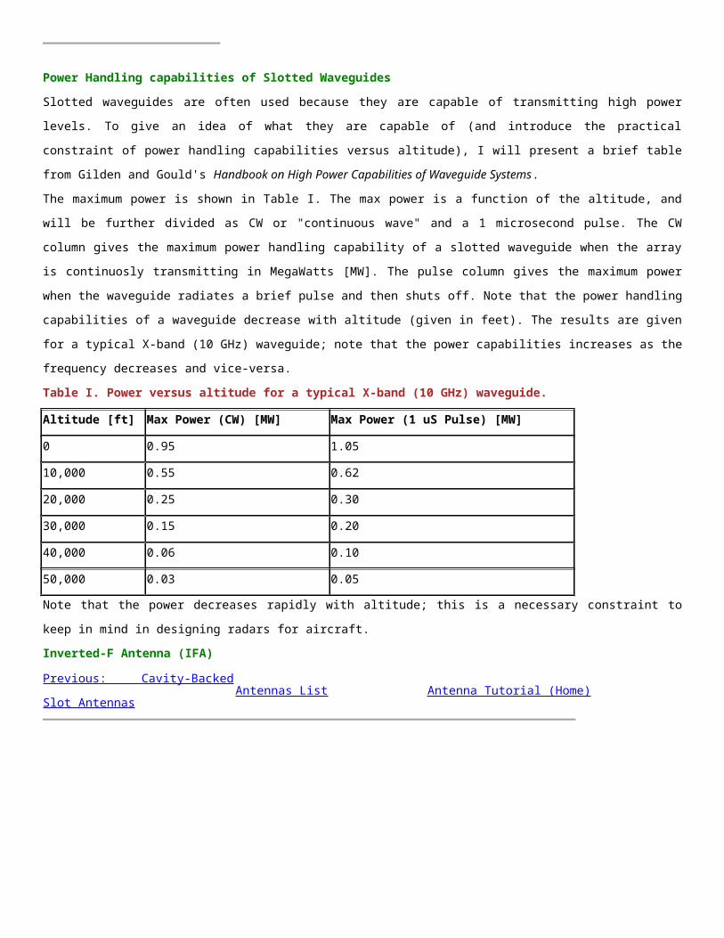
Figure 2. Cell-tower array. These are typically used in groups of 3 (2 receive antennas

and 1 transmit antenna).

The general form of an array can be illustrated as in Figure 3. An origin and coordinate

system are selected, and then the N elements are positioned, each at location given by:

The positions are illustrated in the following Figure.

Figure 3. Geometry of an arbitrary N element antenna array.

Let represent the output from antennas 1 thru N, respectively. The

output from these antennas are most often multiplied by a set of N weights -

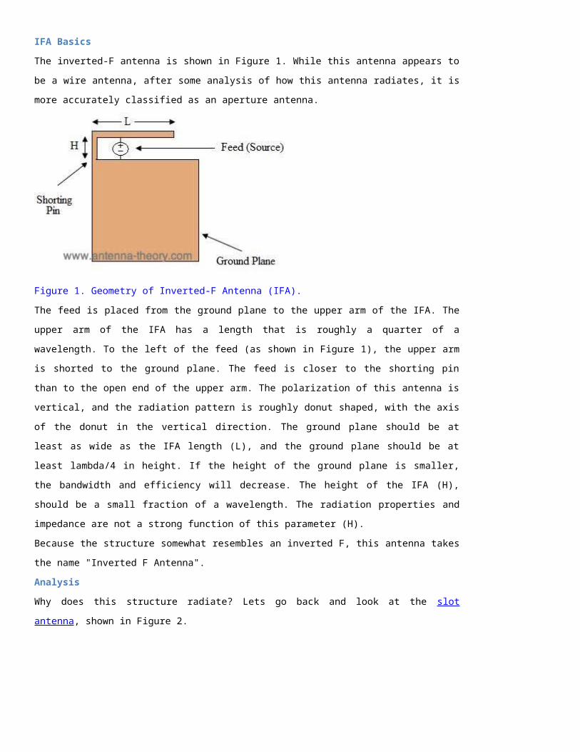
- and added together as shown in Figure 4.

Figure 4. Weighting and summing of signals from the antennas to form the output.

The output of an antenna array can be written succinctly as:

This is what is going on in an antenna array. However, I haven't answered what the

benefits of doing this are. To understand what happens in an antenna array, click the

next link.

To understand the benefits of antenna arrays, we will consider a set of 3-antennas located along the z-

axis, receiving a single arriving from an angle relative to the z-axis of , as shown in Figure 1.

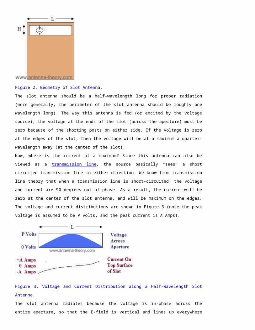
Figure 1. Example 3-element array receiving a plane wave.

The antennas are spaced one-half wavelegnth apart (centered at z=0). The E-field of the plane wave

(assumed to have a constant amplitude everywhere) can be written as:

In the above, k is the wave vector, which specifies the variation of the phase as a function of position.

The (x,y) coordinates of each antenna is (0,0); only the z-coordinate changes for each antenna. Further,

assuming that the antennas are isotropic sensors, the signal received from each antenna is proportional to

the E-field at the antenna location. Hence, for antenna i, the received signal is:

The received signals are distinct by a complex phase factor, which depends on the antenna separations

and the angle of arrival on the plane wave. If the signals are summed together, the result is:

The interesting thing is if the magnitude of Y is plotted versus (the angle of arrival of the plane wave).

The result is given in Figure 2.

Figure 2. Magnitude of the output as a function of the arrival angle.

Figure 2 shows that the array actually processes the signals better in some directions than others. For

instance, the array is most receptive when the angle of arrival is 90 degrees. In contrast, when the angle

of arrival is 45 or 135 degrees, the antenna array has zero output power, no matter how much power is in

the incident plane wave. In this manner, a directional radiation pattern is obtained even though the

antennas were assumed to be isotropic. Even though this was shown for receiving antennas, due to

reciprocity, the transmitting properties would be the same.

The value and utility of an antenna array lies in its ability to determine (or alter) the received

or transmitted power as a function of the arrival angle.

By choosing the weights and geometry of an array properly, the antenna array can be designed to cancel

out energy form undesirable directions and receive energy most sensitively from other directions.

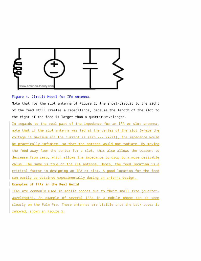
Before considering weight and geometry selection, we first turn to the fundamental function of array

theory, the Array Factor.

The Array Factor

Arrays Main Page Antenna-Theory Home

Intro to Arrays Page 1 Previous: Intro to Arrays Page 2Next: Weighting

Methods

We'll now derive the most important function in array theory - the Array Factor. Consider a

set of N identical antennas oriented in the same direction, each with radiation pattern

given by:

Assume that element i is located at position given by:

Suppose (as in Figure 4 here) that the signals from the elements are each multiplied by a

complex weight ( ) and then summed together to form the array output, Y.

The output of the array will vary based on the angle of arrival of an incident plane wave

(as described here). In this manner, the array itself is a spatial filter - it filters incoming

signals based on their angle of arrival. The output Y is a function of , the arrival

angle of a wave relative to the array. In addition, if the array is transmitting, the radiation

pattern will be identical in shape to the receive pattern, due to reciprocity.

Y can be written as:

where k is the wave vector of the incident wave. The above equation can be factor simply

as:

The quantity AF is the Array Factor. It is a function of the positions of the antennas in the

array and the weights used. By tayloring these parameters the array's performance may

be optimized to achieve desirable properties. For instance, the array can be steered

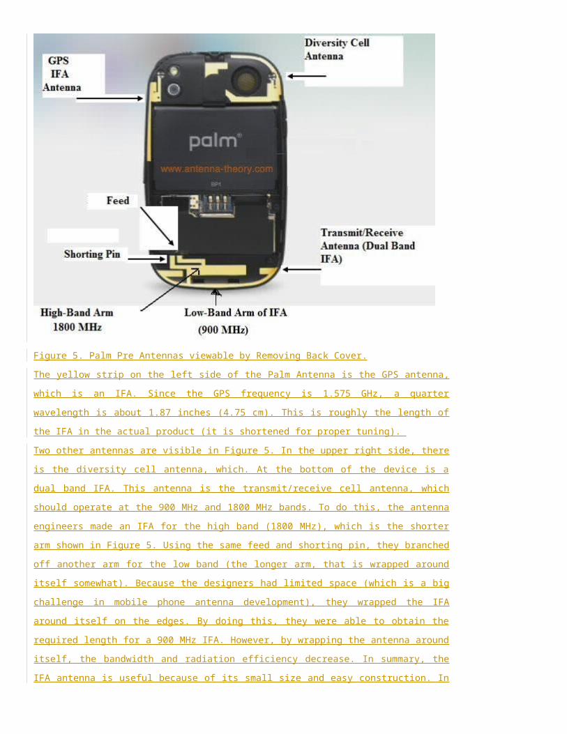
(change the direction of maximum radiation or reception) by changing the weights.

Using the steering vector, the AF can be written compactly as:

In the above, T is the transpose operator. We'll now move on to weighting methods

(selection of the weights) used in antenna arrays, where some of the versatility and power

of antenna arrays will be shown.

Side Note: If the elements are identical (array made up of all the same type of

antennas), and have the same physical orientation (all point or face the same

direction), then the radiation (or reception) pattern for an antenna array is

simply the Array Factor multiplied by the radiation pattern . This

concept is known as pattern multiplication.

A weighting method is a means of selecting the weights that multiply the signals from the antennas:

The weights are fundamental in controlling the behavior of the array. Some methods are now presented,

which also serve to explain the versatility of antenna arrays.

Phased Arrays

Schelkunoff Polynomial Method (Null Placement)

Dolph-Tschebysheff Weights

MMSE Weights

Adaptive Antenna Arrays: The LMS Algorithm

Phased Arrays

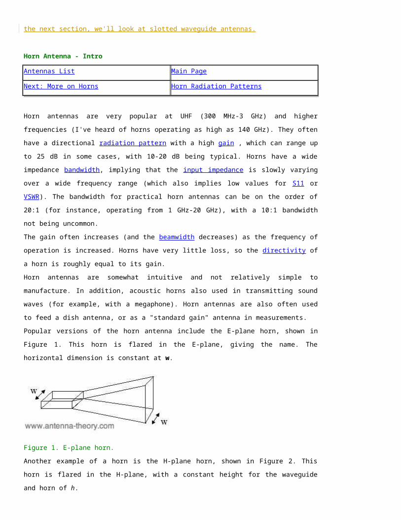
Weighting Methods Antenna-Theory.com Arrays Main Page

Grating LobesAnalysis of Uniform Phased

Arrays

Two Dimensional Phased

Arrays

If a plane wave is incident upon an antenna array (Figure 1), the phase of the signal at

the antennas will be a function of the angle of arrival of the plane wave. If the signals

are then added together, they may add constructively or destructively, depending on

the phases.

Figure 1. The phase of the signal at each element depends on the angle of arrival of the

plane wave.

Lets say that we wanted to receive signals from an angle of 45 degrees, as in Figure 1.

In that case, we would have a good idea of what the phases will be across the antenna

array. Suppose that we multiplied the signal from each antenna by a complex phase (

) that cancelled out the phase change due to the propagation of the wave. Then when

the signals from each antenna are added together to form the output of the array, they

would combine coherently. This is the fundamental principle used in phased arrays - also

known as beam steering.

Lets take an example. Suppose that we had a N=5 element linear array with one-half

wavelength spacing between the antennas (assumed to be isotropic for simplicity). The

positions are each given by:

for n = 0,1,2,3,4. If we want the array to be steered towards 45 degrees

( ), then weights can be applied that are given by:

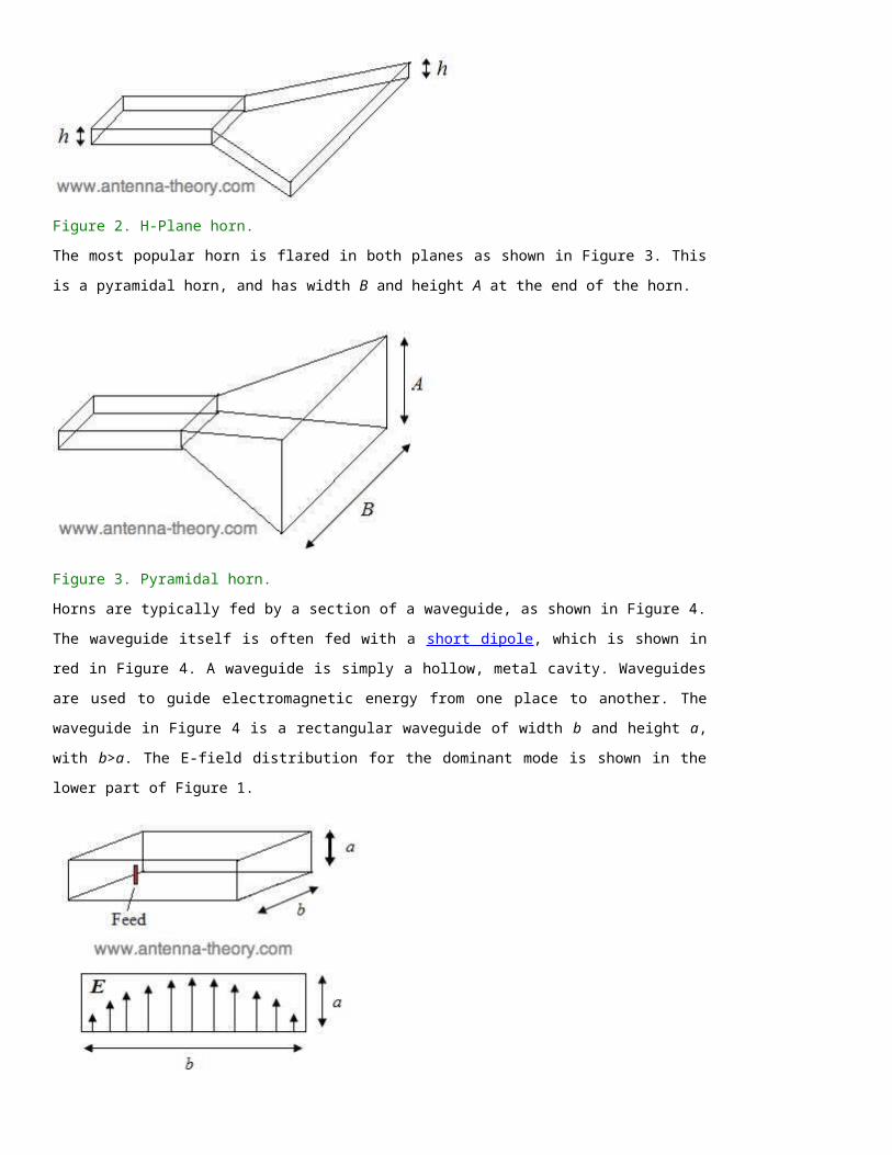
To be absolutely explicit about it, the weight vector can also be written as:

The resulting Array Factor for this array becomes:

In the above, k is the wave vector, v(k) is the steering vector, and N=5.

The array response is the magnitude of the output, as a function of the incident angle of

the plane wave. The array response is identical in form to the radiation pattern of this

array (when the same weights are used). This response is shown in Figure 2.

Figure 2. Response of array versus angle of incidence of a plane wave.

Figure 2 captures the fundamental properties of the designed array. First, the array has

maximum radiation (or reception) in the direction of (img src="thetad.jpg">), as

designed. Second, the array has nulls at roughly 72, 94, 120, and 153 degrees. The null-

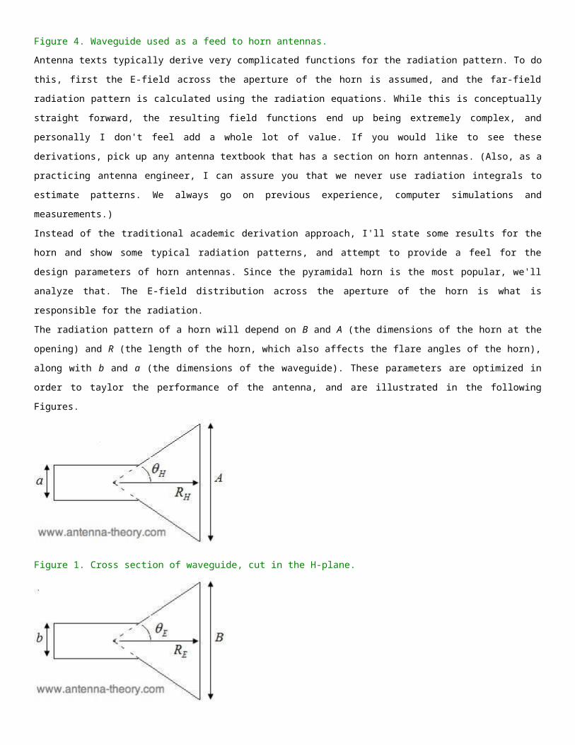
directions are those in which the array completely blocks signals. This array has an

associated HPBW of roughly 30 degrees. Finally, note that the sidelobes are 12 dB below

the peak of the main beam.

Using a phased-weighting scheme is the simplest of all weighting methods. By

employing this method, the array can be steered such that the direction of maximum

reception is in a desired direction. The ease of implementation is responsible for its

widespread use; however, as we'll see, there are better methods of steering (although

the complexity increases).

Grating Lobes

Previous: Phased Arrays Antenna-Theory.com - Home Arrays Main Page

Analysis of Uniform Phased

ArraysMore on Analysis

Two Dimensional Phased

Arrays

We saw previously that a uniformly-spaced array with weights selected to be:

                       (1)

will have the array steered towards the desired direction, . In equation (1), k is the

wave number and d is the spacing between adjacent array elements.

However, it is possible that the array will have equally strong radiation in other

directions. These unintended beams of radiation are known as grating lobes. They

occur in uniformly spaced arrays (arrays with an equal distance between adjacent

elements) when the antenna element separation is too large.

As an example, consider again the situation from the previous page, a group of N=5

uniformly spaced elements with half-wavelength separation on the z-axis.

Supposed that the array is to be steered towards . This means the array is to be

steered along its own axis, in the +z-direction; this type of radiation is known as an

endfire pattern or endfire radiation. The weights can be easily determined from

equation (1) above. The response of the array given these weights is shown in Figure 1.

Recall that the response of the array is mathematically equivalent to the array factor.

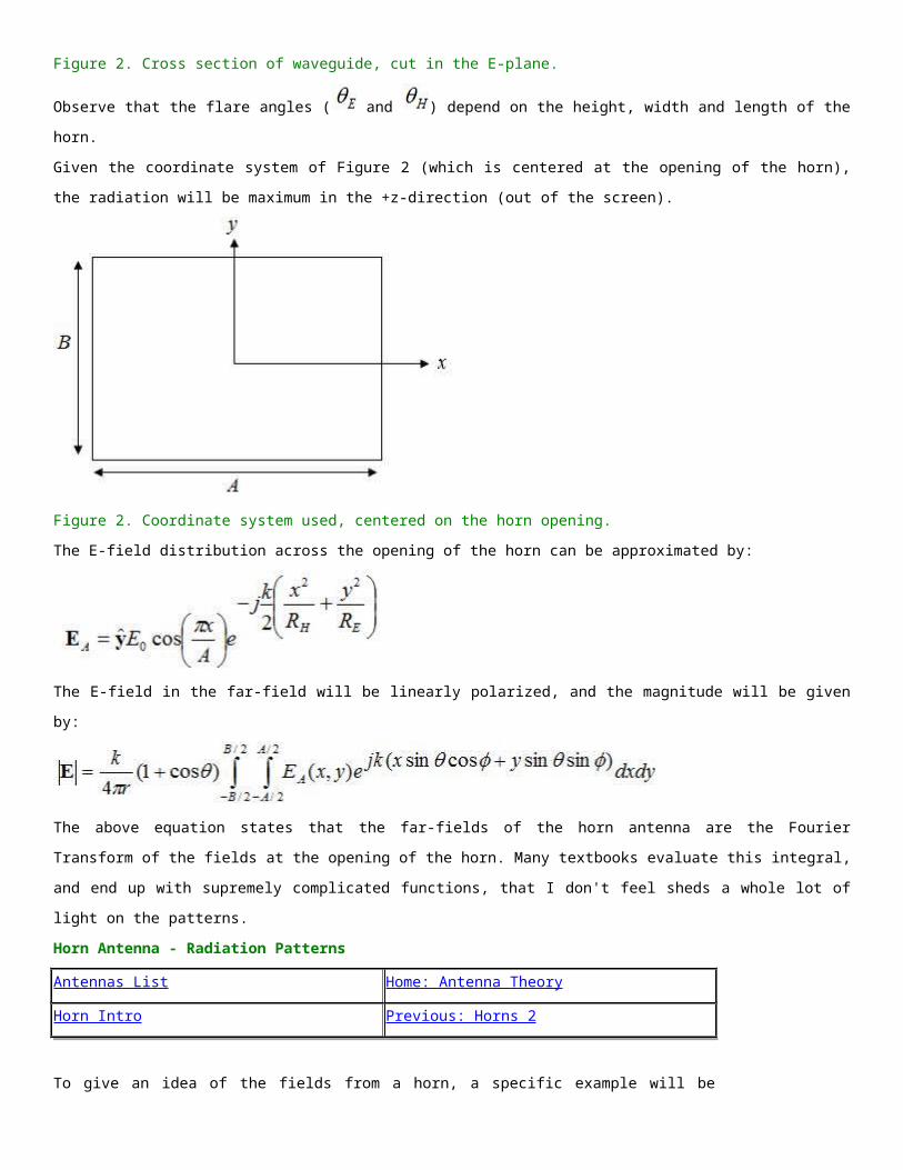
Figure 1. Response of array when weights are steered towards .

Note that in Figure 1, the array does indeed have a response that is maximum towards

the desired direction (0 degrees-or the +z axis). However, the array also produces a lobe

of maximum radiation towards 180 degrees, which was unintended. This lobe is known

as a grating lobe. For uniformly spaced arrays, this can be eliminated by decreasing

the separation between the elements. For non-uniform arrays, grating lobes are much

more difficult to predict.

In the next section, we'll take a more mathematical look at the properties of uniformly

spaced arrays using the phased-steering weighting scheme described by equation (1).

Analysis of Uniform Phased Arrays

Previous: Grating Lobes Antenna-Theory.com - Home Arrays Main Page

Basics of Phased Arrays Grating LobesTwo Dimensional Phased

Arrays

In this page, we'll derive a general equation for the array factor or array response for an

N element uniformly spaced linear array. The weights will be simple phased weights;

when the array is steered towards direction , the weights are given by:

Assuming that element n is at location given by:

This implies that the inter-element spacing is constant and equal to d. Our goal now is to

determine the response of the array when steered towards , when the weights are

chosen using the equation above.

Using the definition of the array factor, we can write:

The above can be simplified by recalling the definition of the wave vector:

Substituting the above equation into the array factor equation,

In the above equation, G is a "dummy variable" that is simply given by:

Recall the following sum formula, which will make our work simple:

The array factor can be rewritten using the above identity as:

Really, we only care about the magnitude of the array factor. Hence, we can factor out

terms from the numerator and denominator that will simplify the results when we take

the magnitude:

Taking the magnitude of the above equation, the multiplying complex exponentials

(which always have a magnitude equal to one) go away. In addition, using the following

general formula for the sin() function:

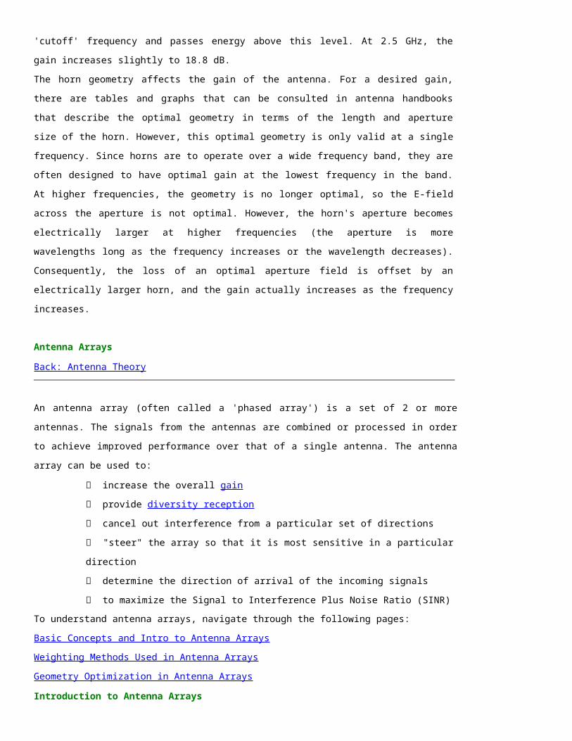
The magnitude of the array factor reduces to:

In the next section, we'll look at understanding this equation (which explains grating

lobes), and extend the results to two-dimensional (planar) arrays.

In the previous page, the general form of the Array Factor for an N element array with uniform spacing of d

and phased tapered weights steered towards was shown to be:

Lets begin by making a variable substitution to simplify the function. Lets rewrite the above equation using

a variable substitution Q as shown below:

For N=5, the |AF| is plotted in Figure 1 as a function of Qd.

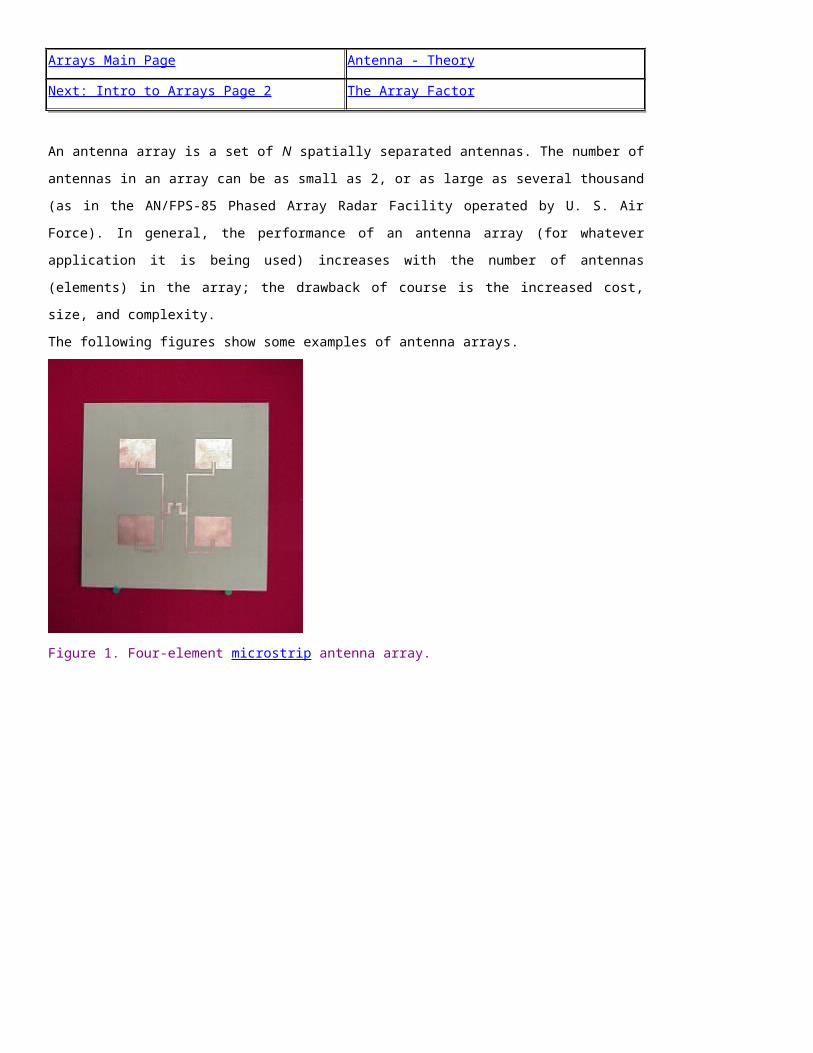
Figure 1. Magnitude of normalized AF for N=5.

For N=10, the |AF| is plotted in Figure 2.

Figure 2. Magnitude of normalized AF for N=10.

Figures 1 and 2 indicate that the |AF| becomes more directional with an increasing number of elements, N.

Secondly, the |AF| has a maximum at Qd=0, which occurs when the observation angle is equal to the

scan angle , which should make sense. Third, the |AF| is a periodic function of Qd. However, note that

Qd can not take any value and be physically realizable. For instance, if is 90 degrees, then Qd is

physically bounded by to be within the range

If is 0 degrees, then Qd is physically bounded by to be within the range

The range of values that are physically realizable are known as the visible region. The values for Qd that

can not occur are in the invisible region. If d = 0.5wavelengths and the array is steered towards 90

degrees, then Qd is bounded between -1.57 and 1.57 ( ). In this range, the AF does not experience

grating lobes , as seen in Figures 1 and 2.

However, if d=0.5 wavelenths and the array is steered towards 0 degrees, then Qd is bounded between 0

and 3.14. In this range, the AF does experience grating lobes within its visible region.

Hence, we can conclude that grating lobes may occur for some scan angles and not others. However, if an

array is steered towards 0 degrees and does not exhibit grating lobes, then they will also not occur for any

other scan angle.

Finally, note that if d is increased, the visible region increases in size. Hence, if d is made to be 2

wavelengths, multiple grating lobes will occur within the visible region. If d is made to be 0.25 wavelengths

or less, the visible region is greatly reduced in size, and no grating lobes will be seen for any scan angle.

Hence, the inter-element spacing strongly controls the AF and whether or not grating lobes appear in

uniformly spaced arrays.

Introduction to Antenna Array Geometry

Arrays Main Page Main Page

2D Hexagonal Arrays Thinned Arrays

We've discussed the basics of antenna arrays and weighting methods in arrays. The

performance of an array will depend on the number of elements in the array (generally

more elements yields better performance), the weighting vector used, and the geometry

of the array. Observing the Array Factor, you will note that the array's output (or

reception pattern) is a strong function of the geometry (positions of the antenna

elements that make up the array).

In this section, we'll discuss array geometry. There are a few basic rules, but its not as

well understood as the weighting methods, which are extensively studied.

In general, if the inter-element spacing between elements for an N element array is

increased, the beamwidth decreases. However, as seen on the grating lobes page,

increasing the size of the array will eventually produce grating lobes - undesirable

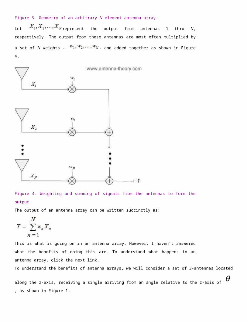
directions of maximum radiation.

For uniformly spaced arrays (either 1D, 2D, or 3D arrays with a constant spacing

between elements), the maximum spacing is a half-wavelength to avoid grating lobes.

This effect is sometimes called "aliasing", which is a term that is borrowed from the

signal processing field. Aliasing occurs when plane waves from two distinct direction of

arrivals (DOAs) produce the same set of phases across the array. Since an antenna array

manipulates signals based on the phase differences that it observes across the array,

aliasing results in the array being unable to distinguish signals from distinct DOAs.

If the array has non-uniform spacing (the spacing between adjacent elements is not

uniform), aliasing can be avoided - particularly if the spacings are not multiples of each

other. For instance, an N=3 element linear array defined by positions will not exhibit

aliasing:

No matter how large the parameter C grows, this 3 element array will not exhibit

aliasing. No two distinct directions of arrival will produce the same set of propagation

delays across the array.

However, the lack of aliasing does not imply that grating lobes will not exist. In fact, if C

is very large (>10), for any scan angle there will exist multiple grating lobes. Hence,

aliasing is not a criteria to focus on; rather, the existance of grating lobes is a more solid

criterian.

Non-uniform arrays do not solve the grating lobe problem, but they do enable extra

degrees of freedom in designing the array. In general, there is no quick method of

determining if an array will exhibit grating lobes. However, any array geometry can be

quickly analyzed to determine if grating lobes will occur.

In the next section, we'll look at the most popular 2D array: the hexagonally sampled

array.

Hexagonal Sampling

Previous: Array Geometry Basics Next: Thinned Arrays

Antenna Arrays Start Page Antennas (Home)

The basic geometry of a 7-element hexagonal array is shown in Figure 1.

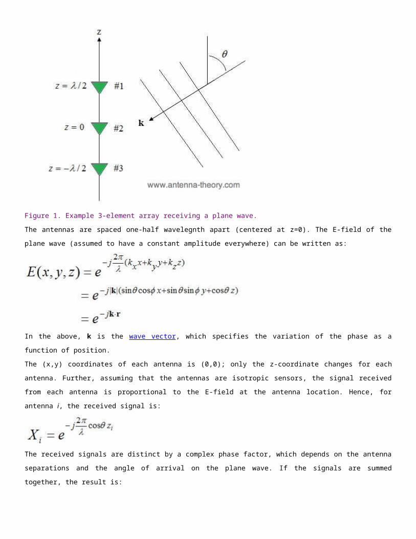
Figure 1. Hexagonal Two-Dimensional Antenna Array.

The hexagonal structure is such that each element is a fixed distance (C in Figure 1)

away from its 6 nearest neighbors. In addition, any 3 adjacent elements forms an

equilateral triangle. This type of spacing is known as hexagonal because the outline of

the outer 6 elements of the array in Figure 1 forms a hexagon; for arrays with more

elements, the hexagons just repeat. Hence, the hexagonal array can have as many

elements as desired.

Why this array? In multidimensional digital signal processing, it is known that sampling

using the hexagonal lattice will produce the least aliasing for band-limited signals. In

addition, the array has somewhat of a circular symmetry, so that the response towards

distinct azimuth angles will not vary by a large degree.

In the author's experience, this array ends up being the optimal geometry for a large

number of problems. For instance, for 2D arrays designed to have the minimum possible

sidelobe level for a fixed beamwidth, the optimal geometry (associated with the optimal

weights) will be a hexagonal array when N=7. In this case, the parameter C is chosen

such that the beamwidth meets the specified criteria and grating lobes do not occur.

As a second example, an adaptive array developed by Raytheon that attempts to block

out interference (or jamming signals) uses a hexagonal geometry. It turns out that by

having a closely spaced sampling (small value of C in Figure 1), the nulls in the radiation

pattern end up being wide, which help the array null out undesired directions.

I don't know of any other definitive reasons for choosing the hexagonal array; however I

do know it is commonly employed. Slotted Waveguide Antennas are often arranged such

that the slots have an approximately hexagonal spacing. In general, if you need to

design the spacing for a 2D array, the hexagonal structure is a great place to start (and

probably end up). In the next section, we'll look at optimizing array geometry.

Thinned Antenna Arrays

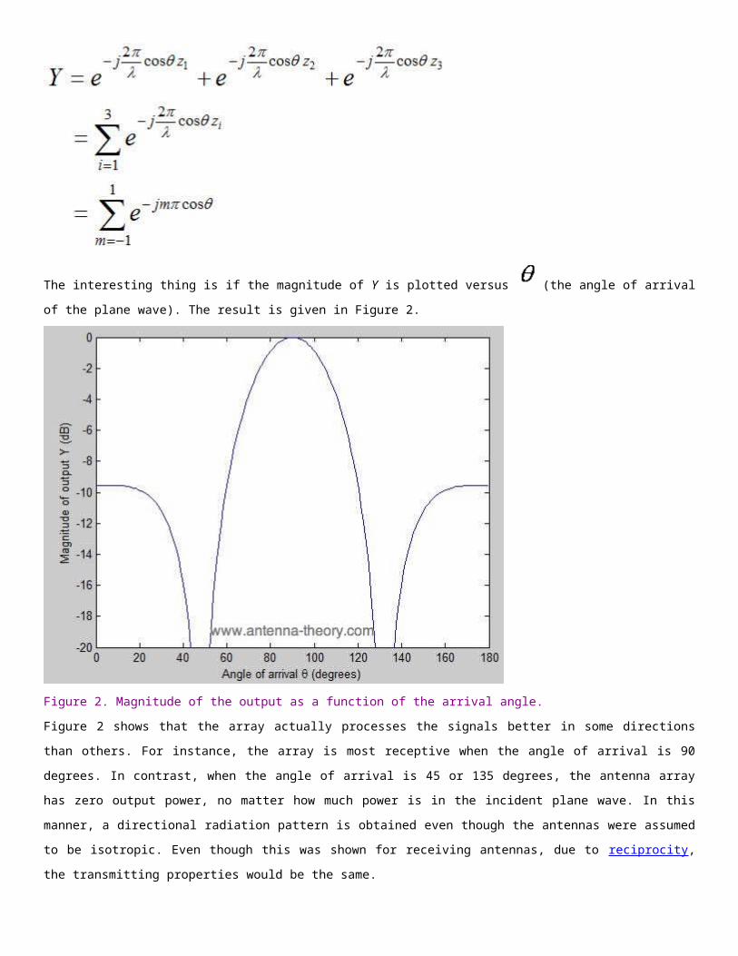
Previous: Hexagonal 2D Arrays Array Geometry Basics

Antenna Arrays Start Page Antennas (Home)

One of the earliest methods of optimizing array geometry dates back to around 1960

and is known as "thinning arrays" or "array thinning". This method is relatively simple. A

large uniformly spaced array (linear or planar) is used as a starting point. Large arrays

are complex to build, have increased fabrication and setup costs, are heavier, etc;

therefore, eliminating antenna elements from the array would be desirable, particularly

if the array's performance is not significantly degraded.

One method of achieving this goal is array thinning - systematically removing elements

without a large degradation in performance. The elements can then be perturbed from

their locations if necessary. To illustrate the utility of this method, a simple example will

be presented.

Consider a 20-element uniformly spaced linear array (with half-wavelength spacing),

with positions given by:

To illustrate the concept of thinned arrays, lets remove some of the elements and

perturb the locations a little, we have a 12 element linear array with positions given by:

Note that both arrays have approximately the same length. Assume that all the weights

for the array are constant and set to one. The resulting Array Factors for both arrays are

plotted in Figure 1.

Figure 1. Magnitude of Array Factor (dB) for Uniform 20-element array and thinned 12-

element array.

Some observations are immediattely apparent after observing Figure 1. First, the peak

gain of the Array Factor decreased for the thinned array. This is because less elements

make up the array; hence this result will always hold for thinned arrays. Second, the

Sidelobe Level and beamwidth are approximately the same for the two cases, except for

large angular separation from the main beam. Hence, the performance of the full

uniform array can be approximately achieved using 40% fewer elements, which is often

highly desirable.

Side Note: The large sidelobes in the thinned array are easily eliminated.

Recall that what is actually radiated by an antenna array is the product

(pattern multiplication) of the Array Factor and the radiation pattern of the

antennas that make up the array. Hence, by choosing an antenna that has low

gain for small and large values of the polar angle theta (such as a simple

dipole antenna, these sidelobes are instantly removed.

In previous example, I just removed some of the antenna elements and twiddled the spacing by hand to

get something I liked. More general methods of array thinning are listed below.

Thinning Based on an Empirical or Analytical Formula: Array thinning can be performed by using a

set rule, which is advantageous because it requires no computation. For instance, array spacing can be

designed to follow the prime number sequence, which leads to non-uniform and sparse spacing:

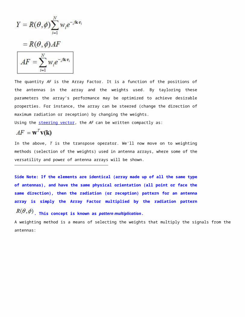
Thinning based on space or density tapering: A successful method of lowering sidelobes in arrays is

to decrease the magnitude of the weights away from the center of the array. This tapering is similar to

"windowing" in digital signal processing. Having a uniform weight set across the array leads to higher

sidelobes than when the weights taper down, in general. The density tapering approach uses uniform

weights for all antennas; however, it removes antenna elements away from the center, in effect having

less energy radiated away from the center of the array, which accomplishes the same effect as state

above.

Statistically thinned arrays: For very large arrays, a statistical method is often used for array tapering.

In this approach, the probability for an element to lie in a particular position is proportional to the desired

weighting for a weight-tapered array. For arrays with a large number of elements, this approach yields

arrays that behave properly and have low sidelobes.

Optimizing Algorithms: Finally, since computers are so computationally fast these days, thinning and

placement optimization is often done via optimization algorithms. Examples include Genetic Algorithms

(GA), the Particle Swarm Optimization (PSO) algorithm, and Simulated Annealing (SA). All of these methods

employ some statistical optimization approach that guesses at the proper elements to remove, then

removes them if this increases the performance of the array. This has been popular in the antenna

literature over the past 15 years, primariliy because it is simple to implement and can achieve interesting

results.

Antenna Measurements

Antennas (Home)

Testing of real antennas is fundamental to antenna theory. All the theory in the world

doesn't add up to a hill of beans if the antennas under test don't perform as desired.

What exactly are we looking for when we test antennas?

Basically, we want to measure many of the fundamental parameters listed on the

Antenna Basics page. The most common and desired measurements are an antenna's

radiation pattern including gain and efficiency, the impedance, the bandwidth, and the

polarization.

The procedures and equipment are described in the following sections:

1. Required Equipment and Ranges

2. Radiaton Pattern and Gain Measurements

3. Phase Measurements

4. Polarization Measurements

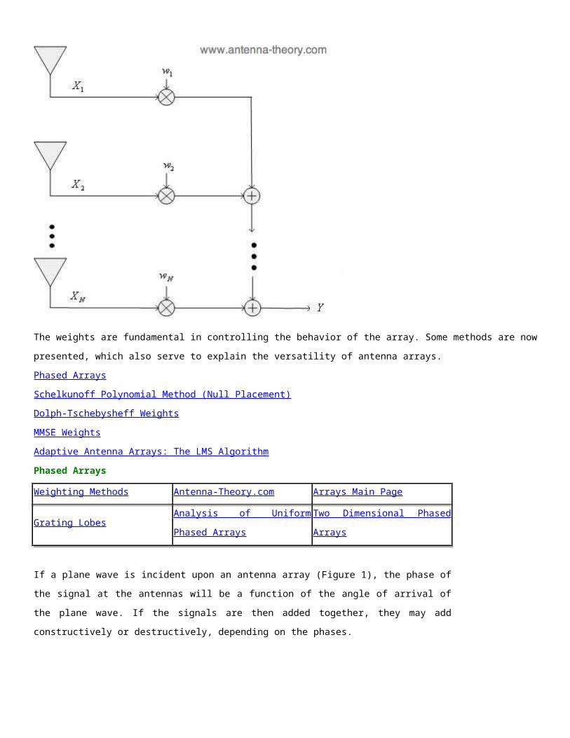
5. Impedance Measurements

6. Scale Model Measurements

Antenna Measurement Equipment

Antennas (Home) Back: Antenna Measurements Home

For test equipment, we will attempt to illuminate the test antenna with a plane wave.

This will be approximated by using a source antenna with no radiation pattern and

characteristics, in such a way that the fields incident upon the test antenna are

approximately planar. More will be discussed about this in the next section. The required

equipment for antenna measurements include:

A source antenna and transmitter - This antenna will have a known pattern that can

be used to illuminate the test antenna

A receiver system - This determines how much power is received by the test antenna

A positioning system - This system is used to rotate the test antenna relative to the

source antenna, to measure the radiation pattern as a function of angle.

A block diagram of the above equipment is shown in Figure 1.

Figure 1. Diagram of required antenna measurement equipment.

These components will be briefly discussed. The Source Antenna should of course

radiate well at the desired test frequency. It must have the desired polarization and a

suitable beamwidth for the given antenna test range. Source antennas are often horn

antennas, or a dipole antenna with a parabolic reflector.

The Transmitting System should be capable of outputing a stable known power. The

output frequency should also be tunable (selectable), and reasonably stable (stable

means that the frequency you get from the transmitter is close to the frequency you

want).

The Receiving System simply needs to determine how much power is received from

the test antenna. This can be done via a simple bolometer, which is a device for

measuring the energy of incident electromagnetic waves. The receiving system can be

more complex, with high quality amplifiers for low power measurements and more

accurate detection devices.

The Positioning System controls the orientation of the test antenna. Since we want to

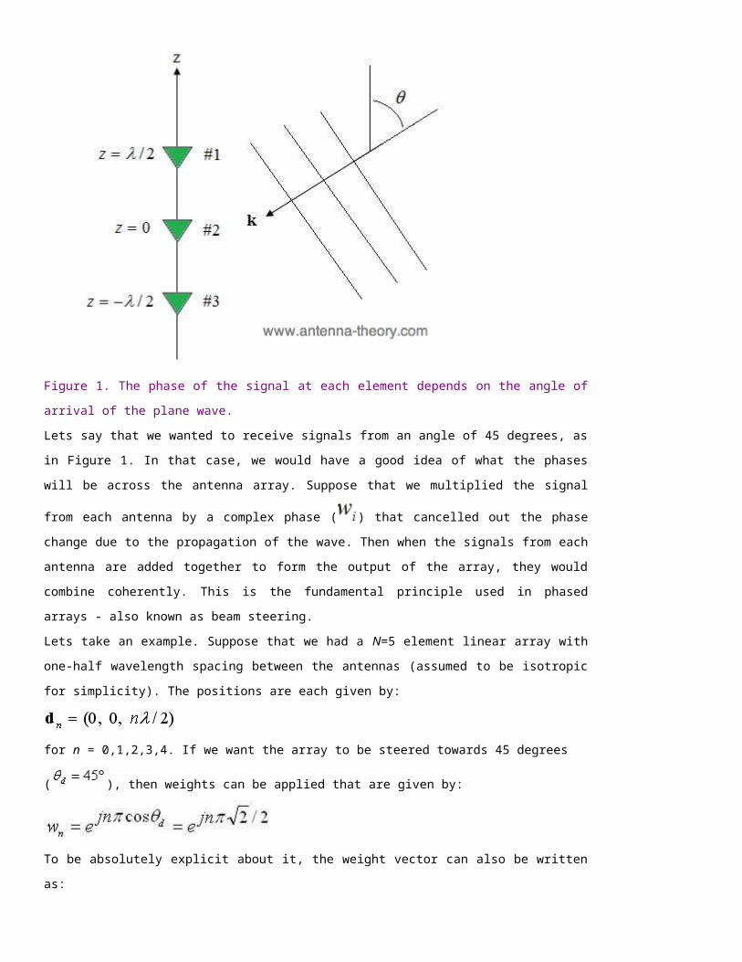
measure the radiation pattern of the test antenna as a function of angle (typically in

spherical coordinates), we need to rotate the test antenna so that the source antenna

illuminates the test antenna from different angles. The positioning system is used for

this purpose.

Once we have all the equipment we need (and an antenna we want to test), we'll need

to place the equipment and perform the test in an antenna range, the subject of the

next section.

Antenna Measurement Equipment

Antennas (Home) Back: Antenna Measurements Home

The first thing we need to do an antenna measurement is a place to perform the

measurement. Maybe you would like to do this in your garage, but the reflections from

the walls, ceilings and floor would make your measurements inaccurate. The ideal

location to perform antenna measurements is somewhere in outer space, where no

reflections can occur. However, because space travel is currently prohibitively

expensive, we will focus on measurement places that are on the surface of the Earth.

There are two main types of ranges, Free Space Ranges and Reflection Ranges.

Reflection ranges are designed such that reflections add together in the test region to

support a roughly planar wave. We will focus on the more common free space ranges.

Free Space Ranges

Free space ranges are antenna measurement locations designed to simulate

measurements that would be performed in space. That is, all reflected waves from

nearby objects and the ground (which are undesirable) are suppressed as much as

possible. The most popular free space ranges are anechoic chambers, elevated ranges,

and the compact range.

Anechoic Chambers

Anechoic chambers are indoor antenna ranges. The walls, ceilings and floor are lined

with special electromagnetic wave absorbering material. Indoor ranges are desirable

because the test conditions can be much more tightly controlled than that of outdoor

ranges. The material is often jagged in shape as well, making these chambers quite

interesting to see. The jagged triangle shapes are designed so that what is reflected

from them tends to spread in random directions, and what is added together from all the

random reflections tends to add incoherently and is thus suppressed further. A picture of

an anechoic chamber is shown in the following picture, along with some test equipment:

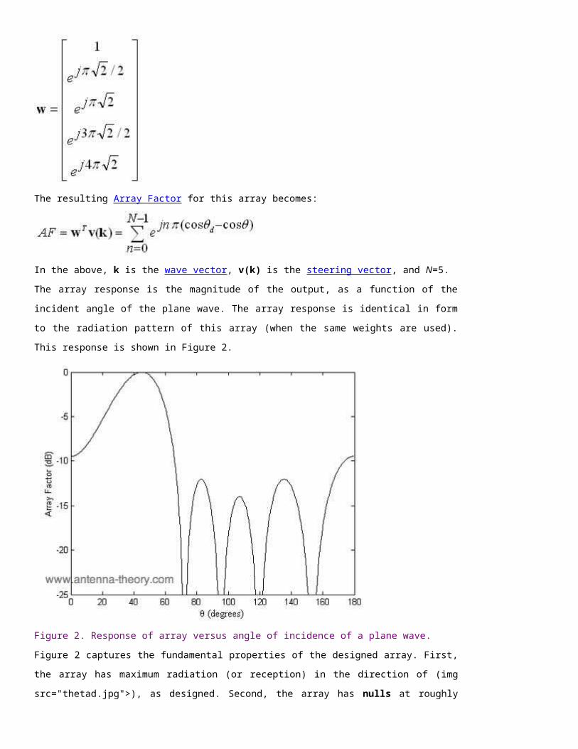
The drawback to anechoic chambers is that they often need to be quite large. Often

antennas need to be several wavelenghts away from each other at a minimum to

simulate far-field conditions. Hence, it is desired to have anechoic chambers as large as

possible, but cost and practical constraints often limit their size. Some defense

contracting companies that measure the Radar Cross Section of large airplanes or other

objects are known to have anechoic chambers the size of basketball courts, although

this is not ordinary. universities with anechoic chambers typically have chambers that

are 3-5 meters in length, width and height. Because of the size constraint, and because

RF absorbing material typically works best at UHF and higher, anechoic chambers are

most often used for frequencies above 300 MHz. Finally, the chamber should also be

large enough that the source antenna's main lobe is not in view of the side walls, ceiling

or floor.

Elevated Ranges

Elevated Ranges are outdoor ranges. In this setup, the source and antenna under test

are mounted above the ground. These antennas can be on mountains, towers, buildings,

or wherever one finds that is suitable. This is often done for very large antennas or at

low frequencies (VHF and below, <100 MHz) where indoor measurements would be

intractable. The basic diagram of an elevated range is shown in Figure 1.

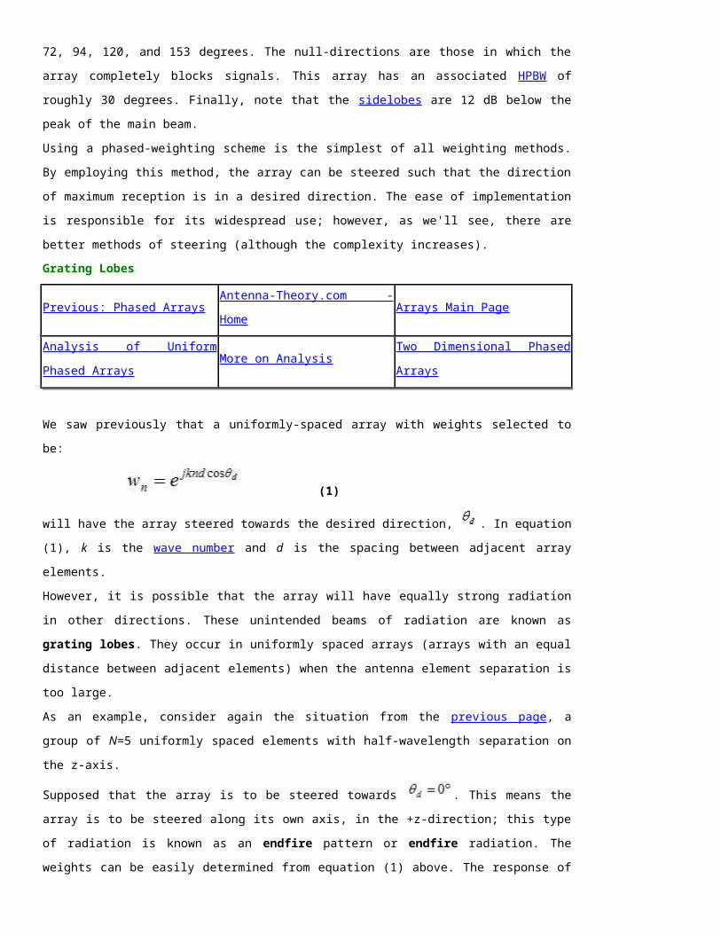
Figure 1. Illustration of elevated range.

The source antenna is not necessarily at a higher elevation than the test antenna, I just

showed it that way here. The line of sight (LOS) between the two antennas (illustrated

by the black ray in Figure 1) must be unobstructed. All other reflections (such as the red

ray reflected from the ground) are undesirable. For elevated ranges, once a source and

test antenna location are determined, the test operators then determine where the

significant reflections will occur, and attempt to minimize the reflections from these

surfaces. Often rf absorbing material is used for this purpose, or other material that

deflects the rays away from the test antenna.

Compact Ranges

The source antenna must be placed in the far field of the test antenna. The reason is

that the wave received by the test antenna should be a plane wave for maximum

accuracy. Since antennas radiate spherical waves, the antenna needs to be sufficiently

far such that the wave radiated from the source antenna is approximately a plane wave

- see Figure 2.

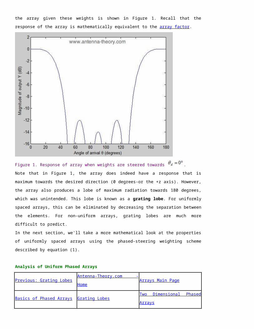
Figure 2. A source antenna radiates a wave with a spherical wavefront.

However, for indoor chambers there is often not enough separation to achieve this. One

method to fix this problem is via a compact range. In this method, a source antenna is

oriented towards a reflector, whose shape is designed to reflect the spherical wave in an

approximately planar manner. This is very similar to the principle upon which a dish

antenna operates. The basic operation is shown in Figure 3.

Figure 3. Compact Range - the spherical waves from the source antenna are reflected to

be planar (collimated).

The length of the parabolic reflector is typically desired to be several times as large as

the test antenna. The source antenna in Figure 3 is offset from the reflector so that it is

not in the way of the reflected rays. Care must also be exercised in order to keep any

direct radiation (mutual coupling) from the source antenna to the test antenna.

Measuring Gain

Antennas (Home) Antenna MeasurementsBack: Measurement of

Antenna Radiation Patterns

On the previous page on measuring radiation patterns, we saw how the radiation pattern

of an antenna can be measured. This is actually the "relative" radiation pattern, in that

we don't know what the peak value of the gain actually is (we're just measuring the

received power, so in a sense can figure out how directive an antenna is and the shape

of the radiation pattern). In this page, we will focus on measuring the peak gain of an

antenna - this information tells us how much power we can hope to receive from a given

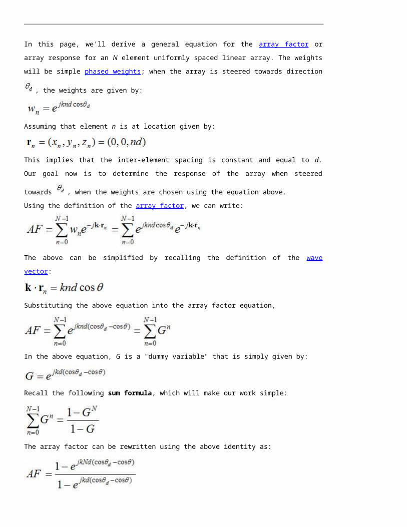
plane wave.

We can measure the peak gain using the Friis Transmission Equation and a "gain

standard" antenna. A gain standard antenna is a test antenna with an accurately known

gain and polarization (typically linear). The most popular types of gain standard

antennas are the thin half-wave dipole antenna (peak gain of 2.15 dB) and the pyramidal

horn antenna (where the peak gain can be accurately calculated and is typically in the

range of 15-25 dB). Consider the test setup shown in Figure 1. In this scenario, a gain

standard antenna is used in the place of the test antenna, with the source antenna

transmitting a fixed amount of power (PT). The gains of both of these antennas are

accurately known.

Figure 1. Record the received power from a gain standard antenna.

From the Friis transmission equation, we know that the power received (PR) is given by:

If we replace the gain standard antenna with our test antenna (as shown in Figure 2),

then the only thing that changes in the above equation is GR - the gain of the receive

antenna. The separation between the source and test antennas is fixed, and the

frequency will be held constant as well.

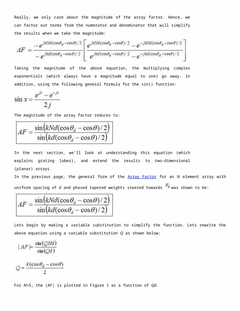
Figure 2. Record the received power with the test antenna (same source antenna).

Let the received power from the test antenna be PR2. If the gain of the test antenna is

higher than the gain of the "gain standard" antenna, then the received power will

increase. Using our measurements, we can easily calculate the gain of the test antenna.

Let Gg be the gain of the "gain standard" antenna, PR be the power received with the

gain antenna under test, and PR2 be the power received with the test antenna. Then the

gain of the test antenna (GT) is (in linear units):

The above equation uses linear units (non-dB). If the gain is to be specified in decibels,

(power received still in Watts), then the equation becomes:

And that is all that needs done to determine the gain for an antenna in a particular

direction.

Efficiency and Directivity

Recall that the directivity can be calculated from the measured radiation pattern without

regard to what the gain is. Typically this can be performed by approximated the integral

as a finite sum, which is pretty simple.

Recall that the efficiency of an antenna is simply the ratio of the peak gain to the peak

directivity:

Hence, once we have measured the radiation pattern and the gain, the efficiency follows

directly from these.

In the next section, we'll look at measuring the phase of an antenna's radiation pattern.

Measuring Phase

Antennas (Home) Antenna Measurements MainBack: Measuring Antenna

Gain

For an antenna's radiation pattern to be completely specified, we need the magnitude of

the power received or transmitted, AND the phase. These measurements should be

specified in two orthogonal directions in order to capture all the components

(polarizations) of the antenna.

For instance, suppose an antenna transmits at frequency f and the fields travelling in the

+y direction at a particular point are seen to be:

The E-fields are orthogonal to the direction of travel in the far field region. The

magnitude of the x-component of the E-field is A and the magnitude of the z-component

of the E-field is B. The phase of the x-component is D and the phase of the z-component

is F (relative to the oscillation at frequency f). If D=F, the components are in phase and

the polarization is linear. If D and F are separated by pi/2 radians (90 degrees) and the

amplitudes are equal, the E-field is circularly polarized.

The phase is a relative quantity - that is, it must be measured relative to some fixed

reference. On this page, we will discuss determining the phase of the fields radiated

from an antenna.

The easiest way to measure phase is the method shown in Figure 1. In this method the

test antenna is used as the source antenna, and another antenna is used to receive the

fields. For this method to work, the observation point is not too far from the test

antenna, so that the source waveform feeding the test antenna can also be run into a

phase measurement box. This box compares the locations of the peaks and valleys of

the received signals and determines the relative phase from this information. The

receive antenna is moved and then the process is repeated.

Figure 1. Measuring the Phase of a Test Antenna When the Observation is 'Near' the

source.

The probe antenna should have good polarization purity, so that it can pick up one

component of the received field. To get the other orthogonal component, it could simply

be rotated or another probe antenna used.

If the test antennas are very far from each other and the reference (source) waveform

can not be fed directly into the phase measurement circuit (this happens at low

frequencies and large outdoor ranges where many wavelengths becomes a large

distance), then a standard antenna with known phase characteristics is used to transmit

a wave, which is used to compare with the received signal from the test antenna.

In the next section, we will look at measuring an antenna's polarization.

Polarization Measurements

Antennas (Home) Back: Phase Measurements

Fundamental to an antenna's radiation pattern is its polarization. On this page, we'll discuss methods

and techniques for determining the polarization of an antenna. Note that the polarization varies

depending on the direction of radiation from an antenna. For instance, a circularly polarized antenna

may be approximately circular only over a narrow beamwidth, and linearly polarized away from the

antenna's main beam (this is often the case for circularly polarized patch antennas).

To perform the measurement, we will use our test antenna as the source. Then we will use a linearly

polarized antenna (typically a half-wave dipole antenna) as the receive antenna. The linearly polarized

receive antenna will be rotated, and the received power recorded as a function of the angle of the

receive antenna. In this manner, we can gain information on the polarization of the test antenna. This

received information only applies to the polarization of the test antenna for the direction in which the

power is received. For a complete description of the polarization of the test antenna, the test antenna

must be rotated so that the polarization can be determined for each direction of interest.

The basic setup for polarization measurements is shown in Figure 1.

Figure 1. Basic setup for antenna polarization measurements.

The power is recorded for the a fixed position (orientation) of the receive antenna, then it is rotated

about the x-axis as shown in Figure 1, and the power is recorded again. This is done for a complete

rotation of the linearly polarized receive antenna.

From this information, a lot can be determined about the polarization of the test antenna. Lets look at a

couple of cases. Suppose that the test antenna is vertically linearly polarized, and that the receive

antenna is also vertically linearly polarized, and that the rotation angle zero has both antennas

polarization matched. Then the output of our experiment, as a function of the rotation angle of the

receive antenna, would look something like the graph shown in Figure 2.

Figure 2. Output of Measurement when the Test Antenna is Linearly Polarized. Left: Rectangular Plot.

Right. Polar Plot.

The plots in Figure 2 give two views of the output. The left side gives an x-y plot of the output. The right

side gives a polar plot, which may be helpful in visualizing the results. Note that the result is periodic -

when the receive antenna is rotated 180 degrees, it is again vertically polarized so that the received

power is identical.

Suppose now that the test antenna was horizontally polarized - again linearly polarized, but initially not

polarization matched to the receive antenna. Then the resulting received power plots would resemble

that shown in Figure 3.

Figure 3. Output measurement of Linearly Polarized Test Antenna (Horizontal Pol).

In this case, we see that the shape of the resulting measurements are the same, but that the peaks of

the received power occur for different angles. As a result, we know that when the test antenna is

linearly polarized, the received power will resemble the shapes shown in Figures 2 and 3, and by

determining the angle in which the received power is at a peak, we can determine the angle of the

linear polarization.

Suppose now that the test antenna was radiating a RHCP (Right Hand Circularly Polarized) wave. If the

test antenna was subject to the same measurement as above, the normalized (make the peak output

power equal to one for simplicity) output power would resemble that of Figure 4.

Figure 4. Output of Measurement when the Test Antenna is Circularly Polarized.

Because a circularly polarized wave has equal amplitude components in two orthogonal directions, the

received power is constant for a rotated linearly polarized antenna (incidentally, this is a feature of

circular polarization that makes it attractive - you don't have to worry about getting the orientation

right). Note also that the received power is the same whether or not the test antenna is left hand

(LHCP) or right hand (RHCP). As a result, this method can determine the type of polarization, but can

not determine the sense of rotation for the polarization. We will need another measurement to

determine this, which is discussed later.

In the meantime, lets look at another example. Suppose the test antenna is elliptically polarized, with a

tilt angle of 45 degrees and an axial ratio of 3 dB. The E-field for this antenna might be described using

the coordinate system of Figure 1 by the equation:

The resulting output of the measurement experiment would be as shown in Figure 5.

Figure 5. Output of Measurement when the Test Antenna is Elliptically Polarized (axial ratio = 3 dB,

major axis along 45 degrees).

Now its getting interesting. Isn't Figure 5 cool? I think so. First, we can tell the tilt angle of the

elliptically polarized wave by where the received power is at a peak - in this case at 45 degrees, which

can be seen from either figure. The other parameter of elliptical polarization - the axial ratio, can be

determined as well from these plots. The ratio of the peak output (in this case 1.0 when the angle is 45

degrees) to the minimum power output (in this case 0.5, when the angle 8s 135 degrees) gives the

axial ratio (1/0.5 = 2 = 3dB). Hence, by simply observing the plots and being aware of the types of

polarization, we can quickly determine the type of polarization for this direction of the test antenna's

radiation pattern. Again, note that we don't know the direction of rotation of the E-field (left or right).

Finally, one more example. Suppose the axial ratio is 9 dB and the major axis of the ellipse is the z-axis.

The result would resemble that of Figure 6.

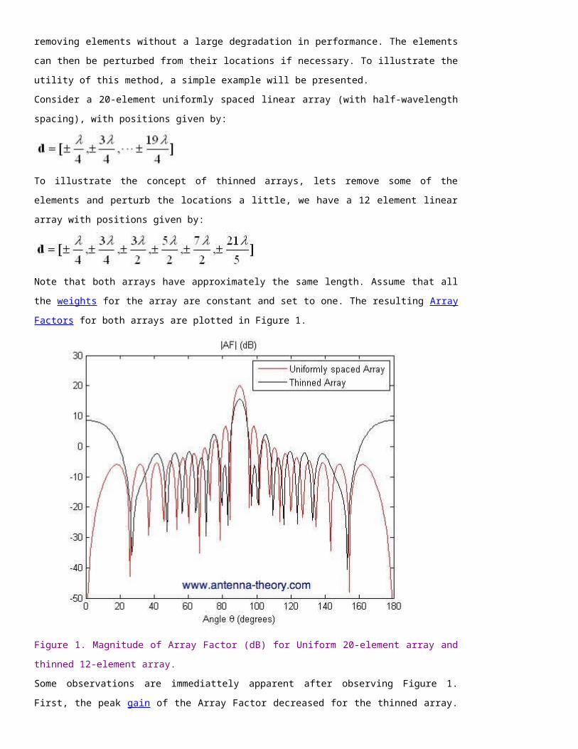
Figure 6. Output of Measurement when the Test Antenna is Elliptically Polarized (axial ratio = 9 dB,

major axis along 0 degrees).

Make sense? If not, read through this page again.

Finally, we would like to determine the sense of polarization for the antenna under test. Suppose that

the test antenna is RHCP, so that we get the output shown in Figure 4. We can't tell from this whether

the result is RHCP or LHCP. A simple approach to determine the sense of rotation in this case is to use

an antenna that is known to be RHCP as the receive antenna. The result is recorded, and then the

measurement is performed again with a receive antenna that is LHCP. The result for the first case

should be much larger than the output for the second case if the test antenna is RHCP. By selecting the

polarization sense based on the output power that is larger, the sense of rotation for the polarization

can be determined. The difficulty in this is that it requires two antennas at the frequency of interest

that are closely RHCP and LHCP, which isn't always easy.

The polarization could also be determined using a combination of phase measurements for two

orthogonal directions in the radiation patterns and then comparing the results along with the

magnitude of the received power. This technique won't be discussed in detail here, but you could

probably piece together the required steps.

Impedance Measurements

Antennas (Home) Back: Polarization Measurements

In this section, we'll be concerned with measuring the impedance of an antenna. As stated

previously, the impedance is fundamental to an antenna that operates at RF frequencies (high

frequency). If the impedance of an antenna is not "close" to that of the transmission line, then

very little power will be transmitted by the antenna (if the antenna is used in the transmit

mode), or very little power will be received by the antenna (if used in the receive mode). Hence,

without proper impedance (or an impedance matching network), out antenna will not work

properly.

Before we begin, I'd like to point out that object placed around the antenna will alter its

radiation pattern. As a result, its input impedance will be influenced by what is around it - i.e.

the environment in which the antenna is tested. Consequently, for the best accuracy the

impedance should be measured in an environment that will most closely resemble where it is

intended to operate. For instance, if a blade antenna (which is basically a dipole shaped like a

paddle) is to be utilized on the top of a fuselage of an aiprlane, the test measurement should be

performed on top of a cylinder type metallic object for maximum accuracy. The term driving

point impedance is the input impedance measured in a particular environment, and self-

impedance is the impedance of an antenna in free space, with no objects around to alter its

radiation pattern.

Fortunately, impedance measurements are pretty easy if you have the right equipment. In this

case, the right equipment is a Vector Network Analyzer (VNA). This is a measuring tool that can

be used to measure the input impedance as a function of frequency. Alternatively, it can plot

S11 (return loss), and the VSWR, both of which are frequency-dependent functions of the

antenna impedance. The Agilent 8510 Vector Network Analyzer is shown in Figure 1.

Figure 1. The popular Agilent (HP) 8510 VNA.

Lets say we want to perform an impedance measurement from 400-500 MHz. Step 1 is to make

sure that our VNA is specified to work over this frequency range. Network Analyzers work over

specified frequency ranges, which go into the low MHz range (30 MHz or so) and up into the

high GigaHertz range (110 GHz or so, depending on how expensive it is). Once we know our

network analyzer is suitable, we can move on.

Next, we need to calibrate the VNA. This is much simpler than it sounds. We will take the cables

that we are using for probes (that connect the VNA to the antenna) and follow a simple

procedure so that the effect of the cables (which act as transmission lines) is calibrated out. To

do this, typically your VNA will be supplied with a "cal kit" which contains a matched load (50

Ohms), an open circuit load and a short circuit load. We look on our VNA and scroll through the

menus till we find a calibration button, and then do what it says. It will ask you to apply the

supplied loads to the end of your cables, and it will record data so that it knows what to expect

with your cables. You will apply the 3 loads as it tells you, and then your done. Its pretty simple,

you don't even need to know what you're doing, just follow the VNA's instructions, and it will

handle all the calculations.

Now, connect the VNA to the antenna under test. Set the frequency range you are interested in

on the VNA. If you don't know how, just mess around with it till you figure it out, there are only

so many buttons and you can't really screw anything up.

If you request output as an S-parameter (S11), then you are measuring the return loss. In this

case, the VNA transmits a small amount of power to your antenna and measures how much

power is reflected back to the VNA. A sample result (from the slotted waveguides page) might

look something like:

Figure 2. Example S11 measurement.

Note that the S-parameter is basically the magnitude of the reflection coefficient, which

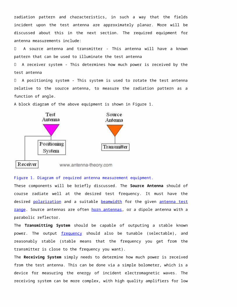
depends on the antenna impedance as well as the impedance of the VNA, which is typically 50

Ohms. So this measurement typically measures how close to 50 Ohms the antenna impedance

is.

Another popular output is for the impedance to be measured on a Smith Chart. A Smith Chart is

basically a graphical way of viewing input impedance (or reflection coefficient) that is easy to

read. The center of the Smith Chart represented zero reflection coefficient, so that the antenna

is perfectly matched to the VNA. The perimeter of the Smith Chart represents a reflection

coefficient with a magnitude of 1 (all power reflected), indicating that the antenna is very poorly

matched to the VNA. The magnitude of the reflection coefficient (which should be small for an

antenna to receive or transmit properly) depends on how far from the center of the Smith Chart

you are. As an example, consider Figure 3. The reflection coefficient is measured across a

frequency range and plotted on a Smith Chart.

Figure 3. Smith Chart Graph of Impedance Measurement versus Frequency.

In Figure 3, the black circular graph is the Smith Chart. The black dot at the center of the Smith

Chart is the point at which there would be zero reflection coefficient, so that the antenna's

impedance is perfectly matched to the generator or receiver. The red curved line is the

measurement. This is the impedance of the antenna, as the frequency is scanned from 2.7 GHz

to 4.5 GHz. Each point on the line represents the impedance at a particular frequency. Points

above the equator of the Smith Chart represent impedances that are inductive - they have a

positive reactance (imaginary part). Points below the equator of the Smith Chart represent

impedances that are capacitive - they have a negative reactance (for instance, the impedance

would be something like Z = R - jX).

To further explain Figure 3, the blue dot below the equator in Figure 3 represents the

impedance at f=4.5 GHz. The distance from the origin is the reflection coefficient, which can be

estimated to have a magnitude of about 0.25 since the dot is 25% of the way from the origin to

the outer perimeter.

As the frequency is decreased, the impedance changes. At f = 3.9 GHz, we have the second

blue dot on the impedance measurement. At this point, the antenna is resonant, which means

the impedance is entirely real. The frequency is scanned down until f=2.7 GHz, producing the

locus of points (the red curve) that represents the antenna impedance over the frequency

range. At f = 2.7 GHz, the impedance is inductive, and the reflection coefficient is about 0.65,

since it is closer to the perimeter of the Smith Chart than to the center.

In summary, the Smith Chart is a useful tool for viewing impedance over a frequency range in a

concise, clear form.

Finally, the magnitude of the impedance could also be measured by measuring the VSWR

(Voltage Standing Wave Ratio). The VSWR is a function of the magnitude of the reflection

coefficient, so no phase information is obtained about the impedance (relative value of

reactance divided by resistance). However, VSWR gives a quick way of estimated how much

power is reflected by an antenna. Consequently, in antenna data sheets, VSWR is often

specified, as in "VSWR: < 3:1 from 100-200 MHz". Using the formula for the VSWR, you can

figure out that this menas that less than half the power is reflected from the antenna over the

specified frequency range.

In summary, there are a bunch of ways to measure impedance, and a lot are a function of

reflected power from the antenna. We care about the impedance of an antenna so that we can

properly transfer the power to the antenna.

In the next Section, we'll look at scale model measurements.

Scale Model Measurements

Antennas (Home) Back: Antenna Impedance Measurements

For the best estimate of an antenna's performance in real conditions, the measurement of the

antenna should be performed in a location that closely resembles the antenna's real world

operating environment. However, in some applications, precise measurements are desired, but

real-world measurements aren't possible. For instance, suppose we are interested in an

antenna's radiation pattern, impedance, etc., and this antenna is to be operated on an airplane.

Or suppose we are interested in the coupling between one antenna to another, both of which

are operating on some random airplane. Its very expensive and difficult to mount the antennas

on an airplane and then make the measurements (particularly the radiation pattern). In

addition, often measurements are desired before the antenna locations are completely

determined, so that we would like to try a few different positions to find an antenna that has a

desired Field of View (FOV - the directions that are not obscured by the aircraft relative to the

antenna) and a desired gain.

One method we can use in this case is that of Scale Model Measurements. In this technique, a

scaled model (typically a much smaller physical model of the actual structure) is used to

represent the platform on which the antenna operates. Now the question is - is this valid? Can

we get proper measurements from a smaller model?

The answer is yes, if we know what we are doing. If you look at the page on frequency, I

mentioned that frequency is one of the fundamental secrets of the universe - every signal can

be represented as a combination of frequencies. Further, all of electromagnetics and antenna

theory are completely described by Maxwell's Equations. If we are riding along a

monochromatic (single frequency) electric field wave (stay with me here) and you encountered

an obstacle, your behavior would only depend on the size of the obstacle in wavelengths. That

is, plane waves respond the same wave to a perfectly conducting circular plate that is 3

wavelengths in diameter, no matter what the frequency.

Hence, lets say we want to know the properties of a monopole antenna at f= 300 MHz

(wavelength is 1 meter). Suppose this antenna is mounted on an airplane that is 30 meters

long, so that the airplane is 30 wavelengths long. Suppose we build a scale model of our

airplane that we can fit in our anechoic chamber, and this airplane model is 3 meters long. If we

want to get the electromagnetic waves to behave the same way as they do on a real airplane at

300 MHz, we need to have the scale model be 30 wavelengths long. Hence, if we operate at f =

3000 MHz (3 GHz, where the wavelength is 0.1 meters), the model is now 30 wavelengths long.

If we scale the monopole antenna by the same factor (10), then our measurements at 3 GHz on

the scaled model will in theory be identical to measurements performed on the actual airplane

at 300 MHz.

Example of a Scaled Model Measurement of an Airplane.

The quality of the results depends on the quality of the model. This method is a valid and often

practiced method of antenna measurements in the aerospace and defense world.

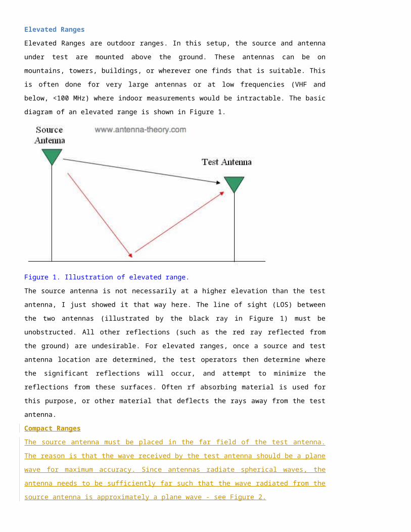
The following table is provided for understanding proper scaling. In the table, the model is

assumed to be scaled down by a factor of n. For instance, in the previous paragraph, the

airplane example had a scaled down model by a factor n=10. As another example, if n=100,

then an L=100 meter real-world object would be represented by a scaled model that is L/n = 1

meter in size.

Table I. Relationship Among Quantities in Scaled Measurements

QuantityScaled

Relationship

Length (L) L/n

Frequency (f) f*n

Permittivity ( )

Permeability ( )

Conductivity ( ) *n

Impedance (Z) Z

Gain (G) G

Radar Cross Section

(A)A*n^2

Capacitance (C) C/n

Inductance (L) L/n

Table I is the result of working through the math in Maxwell's Equations. The good news is that

some properties do not need scaled at all, particularly the permittivity and permeability (if you

are modeling dielectrics or magnetic materials). In addition, the antenna impedance and gain do

not need scaled either, which is a good thing. However, some things like conducitivity need to

be increased by a factor of n in the scaled model. One way to understand this is to note that the

resistance of the scaled model should be constant, and resistance is proportional to the

conductivity of the object times the length divided by the cross sectional area. If the length goes

down by a factor of n, and the cross sectional area goes down by a factor of n^2, then for

constant resistance we require that the conductivity increases by a factor of n on the scaled

model. Typically, the real world airplane has a shell that has high conductivity (metals). Hence,

care needs exercised that the conductivity of the model is as high as possible. This can be done

with polished high quality metals for the scaled model.

Measuring Radiation Pattern and an Antenna's Gain

Antennas (Home)Antenna Measurements

Home

Previous: Measurements

Ranges

Now that we have our measurement equipment and an antenna range, we can perform

some measurements. We will use the source antenna to illuminate the antenna under

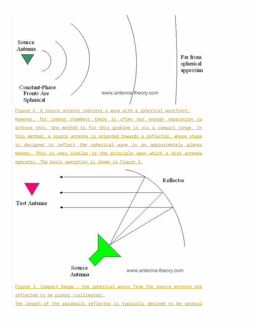
test with a plane wave from a specific direction. The polarization and gain (for the fields

radiated toward the test antenna) of the source antenna should be known.

Due to reciprocity, the radiation pattern from the test antenna is the same for both the

receive and transmit modes. Consequently, we can measure the radiation pattern in the

receive mode for the test antenna.

The test antenna is rotated using the test antenna's positioning system. The received

power is recorded at each position. In this manner, the magnitude of the radiation

pattern of the test antenna can be determined. We will discuss phase measurements

and polarization measurements later.

The coordinate system of choice for the radiation pattern is spherical coordinates.

Measurement Example

An example should make the process reasonably clear. Suppose the radiation pattern of

a microstrip antenna is to be obtained. As is usual, lets let the direction the patch faces

('normal' to the surface of the patch) be towards the z-axis. Suppose the source antenna

illuminates the test antenna from +y-direction, as shown in Figure 1.

Figure 1. A patch antenna oriented towards the z-axis with a Source illumination from

the +y-direction.

In Figure 1, the received power for this case represents the power from the angle:

. We record this power, change the position and record again. Recall

that we only rotate the test antenna, hence it is at the same distance from the source

antenna. The source power again comes from the same direction. Suppose we want to

measure the radiation pattern normal to the patch's surface (straight above the patch).

Then the measurement would look as shown in Figure 2.

Figure 2. A patch antenna rotated to measure the radiation power at normal incidence.

In Figure 2, the positioning system rotating the antenna such that it faces the source of

illumination. In this case, the received power comes from direction . So

by rotating the antenna, we can obtain "cuts" of the radiation pattern - for instance the

E-plane cut or the H-plane cut. A "great circle" cut is when =0 and is allowed to vary

from 0 to 360 degrees. Another common radiation pattern cut (a cut is a 2d 'slice' of a

3d radiation pattern) is when is fixed and varies from 0 to 180 degrees. By

measuring the radiation pattern along certain slices or cuts, the 3d radiation pattern can

be determined.

It must be stressed that the resulting radiation pattern is correct for a given polarization

of the source antenna. For instance, if the source is horizontally polarized (see

polarization of plane waves), and the test antenna is vertically polarized, the resulting

radiation pattern will be zero everywhere. Hence, the radiation patterns are sometimes

classified as H-pol (horizontal polarization) or V-pol (vertical polarization). See also cross-

polarization.

In addition, the radiation pattern is a function of frequency. As a result, the measured

radiation pattern is only valid at the frequency the source antenna is transmitting at. To

obtain broadband measurements, the frequency transmitted must be varied to obtain

this information.