G e o m e t r i c a l P a r a m e t e r s E x t r a c t i o n f r o m D i s c r e t e P a t h s

Anne Vialard

Laboratoire Bordelais de Recherche en Informat ique - URA 1304

Universitd Bordeaux I 351, cours de la Libdration

F-33~05 Talence, France

{Anne. Vialard}@labri. u-bordeaux, fr

Abstract. We present in this paper the advantages of using the model of Euclidean paths ]or the geometrical analysis of a discrete curve. The Euclidean paths are a semi-continuous representation of a discrete path providing a good approximation of the underlying real curve. We describe the use of this model to obtain accurate estimations of lenght, tangent orientation and curvature.

Keywords. Discrete Paths, Euclidean Paths, lenght estimation, curvature es- timation.

1 I n t r o d u c t i o n

The evaluation of geometrical properties of discrete objects plays an important role in image analysis. The most used properties of a discrete curve are its lenght, the tangent orientation and the curvature value at each point. They allow us to analyse a discrete object by characterizing its boundary.

Lenght estimation of discrete curves has been studied in [3]. Curvature esti- mation is particularly important as a quantitative value for object recognition from digital images. The qualitative value of curvature is used for example in edge detection algorithms based on active contours [9, 5].

We present in this paper a representation of 8-connected discrete paths that is well suited to geometrical parameter extraction. This model has been called Euclidean paths. A similar representation for 4-connected discrete paths has been detailed in a previous paper [1]. We have studied the 8-connected case to compare our results with existing methods.

The Euclidean paths construction consists in smoothing the original discrete curve without any loss in information. This provides a good approximation of the real curve underlying the discrete curve. Moreover the proposed construction of Euclidean paths provides a good estimation of tangent orientation along the discrete curve. The qualities of our contour model allow us to improve existing discrete methods for estimating the geometrical characteristics of discrete curves.

In section 2 we briefly present the definition and construction of Euclidean paths associated to 8-connected discrete curves. We then focus on lenght esti- mation (section 3) and curvature estimation (section 4).

25

Note that we have used the technique of best ajustment to obtain the discrete representations of geometrical objects such as circles, rectangles and ellipses.

2 Euclidean paths for 8-connexity

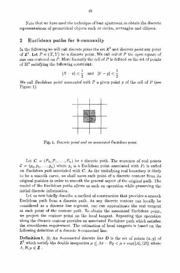
In the following we will call discrete plane the set Z 2 and discrete point any point of Z 2. Let P = (X, Y) be a discrete point. We call cell of P the open square of size one centered on P. More formally the cell of P is defined as the set of points of ]R 2 satisfying the following constraint:

1 1 I X - x[ < ~ and IY- y[ <

We call Euclidean point associated with P a given point p of the cell of P (see Figure 1).

i

t

Fig. 1. Discrete point and an associated Euclidean point.

Let C = (P0, P 1 , . . . , Pn) be a discrete path. The sequence of real points g = ( P o , P l , . . . , P , ) where Pi is a Euclidean point associated with Pi is called an Euclidean path associated with C. As the underlying real boundary is likely to be a smooth curve, we shall move each point of a discrete contour from its original position in order to smooth the general aspect of the original path. The model of the Euclidean paths allows us such an operation while preserving the initial discrete information.

Let us now briefly describe a method of construction that provides a smooth Euclidean path from a discrete path. As any discrete contour can locally be considered as a discrete line segment, one can approximate the real tangent at each point of the contour path. To obtain the associated Euclidean point, we project the contour point on the local tangent. Repeating this operation along the discrete contour provides an associated Euclidean path which satisfies the smoothness requirement. The estimation of local tangents is based on the following definition of a discrete 8-connected line.

D e f i n i t i o n l . [6] An 8-connected discrete line D is the set of points (x, y) of Z 2 which satisfy the double inequation/1 < g x - B y < 1~ + sup(IA], tB[) where A , B , # 6 Z .

26

The rational ~ is the slope of D and the integer p describes its position in the discrete plane.

Let us consider an 8-connected discrete line D and a given point P of D . Let (A, B, #) be the characteristics of D calculated in the local coordinates system of origin P. Without any loss of generality, we suppose here 0 _< A _< B ( D is located in the first octant). The other cases can be inferred by using symmetries. The equation of D is now # _< A x - By < g + B.

~-2~-B It Let p be the real point of coordinates (x, y) = (0, a) with a = 2B " can be shown that a verifies --~ < c~ < �89 In other words, p is a Euclidean point associated with P. One can consider p as a vertical projection of P on the real line • of equation A l - 2 , - B �9 �9 y = g x + 2B . Another pro3ectlon has been proposed in [4]. The vertical projection tends to equalize the distances between Euclidean points. This construction of a Euclidean point associated with a point of a discrete line is illustrated on Figure 2.

P

D

local tangent

Fig. 2. Construction of an Euclidean point

Let us now consider a point P of a discrete path C. We use a vectorization algorithm in order to find the longest discrete line segment of C around P. We apply the line recognition process symmetrically around P to extract a segment corresponding to the intuitive notion of the tangent at P. We use an adapted version of the vectorization algorithm of Debled and Reveilles [2] to obtain the characteristics of the recognized discrete line [1]. The real line 7? associated to the recognized line D is an approximation of the real tangent at P. The characteristics of the discrete tangent at P and the projection described above are used to compute the Euclidean point associated with P.

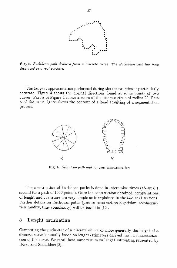
An example of Euclidean path associated with a discrete closed curve is presented on Figure 3. It shows the smooting quality of the method. We can also remark that the angular points are preserved.

27

Fig. 3. Euclidean path deduced from a discrete curve. The Euclidean path has been displayed as a real polyline.

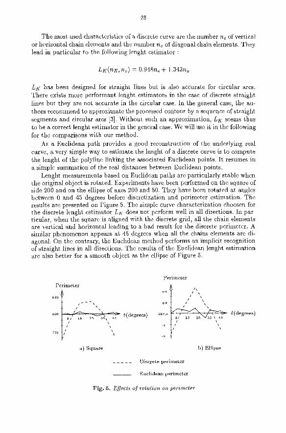
The tangent approximation performed during the construction is particularly accurate. Figure 4 shows the normal directions found at some points of two curves. Part a of Figure 4 shows a zoom of the discrete circle of radius 20. Part b of the same figure shows the contour of a head resulting of a segmentation process.

a) b)

Fig. 4. Euclidean path and tangent approximation

The construction of Euclidean paths is done in interactive times (about 0.1 second for a path of 1000 points). Once the construction obtained, computations of lenght and curvature are very simple as is explained in the two next sections. Further details on Euclidean paths (precise construction algorithm, reconstruc- tion quality, time complexity) will be found in [10].

3 Lenght es t imat ion

Computing the perimeter of a discrete object or more generally the lenght of a discrete curve is usually based on lenght estimators derived from a characteriza- tion of the curve. We recall here some results on lenght estimating presented by Dorst and Smeulders [3] .

28

The most used characteristics of a discrete curve are the number n~ of vertical or horizontal chain elements and the number no of diagonal chain elements. They lead in particular to the following lenght estimator :

LK(r~E,no) = 0.948ne + 1.343no

LK has been designed for straight lines but is also accurate for circular arcs. There exists more performant lenght estimators in the case of discrete straight lines but they are not accurate in the circular case. In the general case, the au- thors recommend to approximate the processed contour by a sequence of straight segments and circular arcs [3]. Without such an approximation, LK seems thus to be a correct lenght estimator in the general case. We will use it in the following for the comparisons with our method.

As a Euclidean path provides a good reconstruction of the underlying real curve, a very simple way to estimate the lenght of a discrete curve is to compute the lenght of the polyline linking the associated Euclidean points. It resumes in a simple summation of the real distances between Euclidean points.

Lenght measurements based on Euclidean paths are particularly stable when the original object is rotated. Experiments have been performed on the square of side 200 and on the ellipse of axes 200 and 50. They have been rotated at angles between 0 and 45 degrees before discretization and perimeter estimation. The results are presented on Figure 5. The simple curve characterization choosen for the discrete lenght estimator LK does not perform well in all directions. In par- ticular, when the square is aligned with the discrete grid, all the chain elements are vertical and horizontal leading to a bad result for the discrete perimeter. A similar phenomenon appears at 45 degrees when all the chains elements are di- agonal. On the contrary, the Euclidean method performs an implicit recognition of straight lines in all directions. The results of the Euclidean lenght estimation are also better for a smooth object as the ellipse of Figure 5.

Perimeter

8 3 0

8 0 0

770

--~"7"~ .~/..~\ ~-"~f 0(degrees) 5 / 15 25 35~ 45 / \

\

a) Square

Perimeter

-t-8 ~ , ' I x ,

! Y \ / \

+ 4 l / \

5 / 15 25 35 "~ 45

.8 t

b) Ellipse

Discrete perimeter

Euclidean perimeter

Fig. 5. Effects of rotation on perimeter

29

Experiments on perimeter have also been performed on discrete circles. In that case the discrete est imator LK performs well since all directions are equally represented. We have used the following error measurement :

iperi~ - pe t i t I err = �9 100%

perir

where peri~ is the estimated perimeter and peri~ is the real perimeter. For circles of radii from 5 to 50 we have obtained an error between 0.03% and 0.92% with the Euclidean method. For the discrete approximation the error falls between 0.28% and 2.77%. In this case, the improvement provided by the Euclidean method is not really significant since the discrete measurement is already accurate.

The three main advantages of the Euclidean lenght estimation are the fol- lowing. The lenght estimation is little dependent on the position of the object on the discrete grid. Moreover it is a general method whitch has not been designed for particular cases. It allows us an accurate estimation for polygons as well as for smooth objects. It is also suited to 4-connected discrete contours [1]. Discrete lenght estimators are not adapted to that late case.

Surface estimation can also be computed from a Euclidean pa th as the surface of the Euclidean polyline. The discrete method for surface estimation consists in computing the surface of the polygon linking the discrete points [7]. The Eu- clidean method does not lead to a significant improvement of surface estimation since the discrete method provides good results. As a mat ter of fact the surface of an object is little affected by small variations along the contour all the more if the object is large. Moreover the irregularities of a discrete contour tend to cancel each other out in the case of surface computat ion which is not the case for lenght estimation where errors cumulate.

4 C u r v a t u r e m e a s u r e m e n t

The principal approaches for computing curvature along a discrete contour are presented in a survey by Worring and Smeulders [11]. They differ in the choosen definition of curvature. As a mat ter of fact the curvature at a point of a curve can be defined in three different ways :

1- as the derivative of the tangent orientation 2- as the norm of the second derivative of the curve considered as a pa th 3- as the inverse of the osculating circle radius

Although these three definitions are equivalent in the continuous case, they differ in the discrete case. Worring and Smeulders show that the best existing method is a method based on tangent orientation and called resampling method. It con- sists in computing curvature by a Gaussian differential filtering applied to the estimated tangent orientations.

Before the curvature estimation process, the discrete contour is resampled [8]. The resampling process aims at improving the estimation of the tangent orien- tat ion and reduces the distance differences between the contour points whitch is

30

important for the filtering process. Let C be a discrete contour of n + 1 points and consider the polyline linking the points of C. The resampled contour T~ = (r0, r l , . . . , r~) deduced from C is composed of n + 1 equidistant real points belonging to the polyline. Let us denote by (x~(i), yr(i)) the coordinates of ri. The estimated curvature g(i) at ri is given by definition 2.

D e f i n i t i o n 2. [11] _ o ( i ) �9

1.1107

with O(i) = t a n - l ( y~(i § 1) - y-(i) x ~ ( i + 1) x . ( i ) )

i --i 2 a n d = e x p m , =

The coefficient 1.1107 represents the average distance between two points of the discrete contour. The window size is set at m = 3c~ to limit the truncation error on the Gaussian function.

Figure 6 shows the curvature computed with the resampling method along a circle of radius 50. Two window sizes have been used. We can state from this figure that the resampling method is inaccurate for a small window size (~r = 1). A larger window size provides a smoother result deriving from the convolution of definition 2.

Curvature Curvature

0 .2

0 .1

0.0~ 0

-0 .1

-0 .2

a = l 0 , 2 '

0 . 1

0.02 0

-0 .1

-0 .2

o r = 3

Fig. 6. Resampling method - Curvature along a circle of radius 50

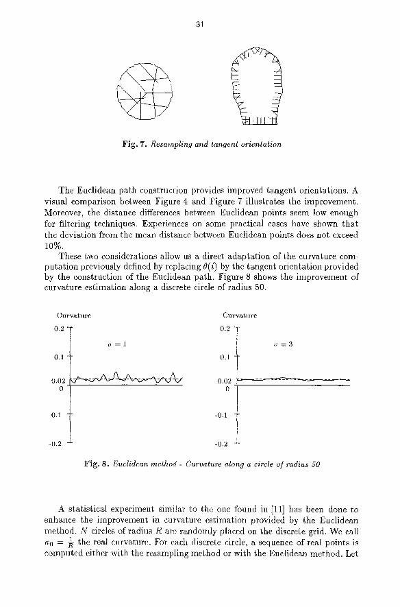
The resampling process improves the estimation of tangent orientation in comparison with a direct estimation from the chain code. However tangent esti- mation remains inaccurate. Figure 7 shows the normal directions at some points of two curves already presented in Figure 4.

31

Fig. 7. Resampling and tangent orientation

The Euclidean path construction provides improved tangent orientations. A visual comparison between Figure 4 and Figure 7 illustrates the improvement. Moreover, the distance differences between Euclidean points seem low enough for filtering techniques. Experiences on some practical cases have shown that the deviation from the mean distance between Euclidean points does not exceed io%.

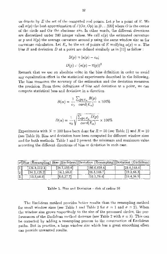
These two considerations allow us a direct adaptation of the curvature com- putation previously defined by replacing O(i) by the tangent orientation provided by the construction of the Euclidean path. Figure 8 shows the improvement of curvature estimation along a discrete circle of radius 50.

Curvature Curvature

0.2 0.2

0.1

0.02 0

-0.1

-0.2

c~=l

0.1

0.02 0

-0.1

c~=3

-0.2

Fig. 8. Euclidean method - Curvature along a circle of radius 50

A statistical experiment similar to the one found in [11] has been done to enhance the improvement in curvature estimation provided by the Euclidean method. N circles of radius R are randomly placed on the discrete grid. We call ~0 = 1 the real curvature. For each discrete circle, a sequence of real points is computed either with the resampling method or with the Euclidean method. Let

32

us denote by E the set of the computed real points. Let p be a point of E. We call a(p) the best approximation o f / ( O x , Op) in [0 . . . 239] where O is the center of the circle and Oz the abscissae axe. In other words, the different directions are diseretized under 240 integer values. We call ~(p) the estimated curvature at p and g(p) the average curvature around p using the same window size as for curvature calculation. Let E~ be the set of points of E verifying a(p) = a. The bias B and deviation D at a point are defined similarly as in [11] as follow :

B(p) = ]~(p) - ~o[

z ) ( v ) = -

Remark that we use an absolute value in the bias definition in order to avoid any equalization effect in the statistical experiments described in the following. The bias measures the accuracy of the estimation and the deviation measures the precision. From these definitions of bias and deviation at a point, we can compute statistical bias and deviation in a direction.

B(a) = 1 ~---,pet~ B(p) ~o eard(E~) x 100%

D( I = • 100%

Experiments with N = 100 have been done for R = 50 (see Table 1) and R = 10 (see Table 2). Bias and deviation have been computed for different window sizes and for both methods. Table 1 and 2 present the minimum and max imum value according the different directions of bias or deviation in each case.

~Bias (Resampling) Bias (Euclidean)

[126"8'512"11

Deviation (Resampling) Deviation (Euclidean)

[28.7,150.6] [180.6,658.6] [23.6,148.6] [44.3,148.7] [19.2,66.3] [34.2,125.2] [14.1,50.0]

[13.5,60.0] [8.6,27.7] [16.5,70.4] [10.4,36.9]

Table 1. Bias and Deviation - disk of radius 50

The Euclidean method provides better results than the resampling method for small window sizes (see Table 1 and Table 2 for cr = 1 and ~r = 2). When the window size grows respectively to the size of the processed circles, the per- formances of the Euclidean method decrease (see Table 2 with r = 3). This can be corrected by adding a resampling process to the construction of Euclidean paths. But in practice, a large window size which has a great smoothing effect can provide unwanted results.

33

IcrllBias (Resampl ing) lBias (Euclidean) : Deviat ion (Resampling)

1 [38.5,83.5] 2 [9.4,18.2] 3 [3.6,5.5]

[17.0,45.0] [52.7,108.1]

Deviat ion (Eucl idean)

[22.9,63.0] [5.5,13.5] [12.6,23.2] [7.9,20.4] [2.5,6.5] [4.1,7.3] [3.6,8.6]

T a b l e 2. Bias and Deviat ion - disk of radius 10

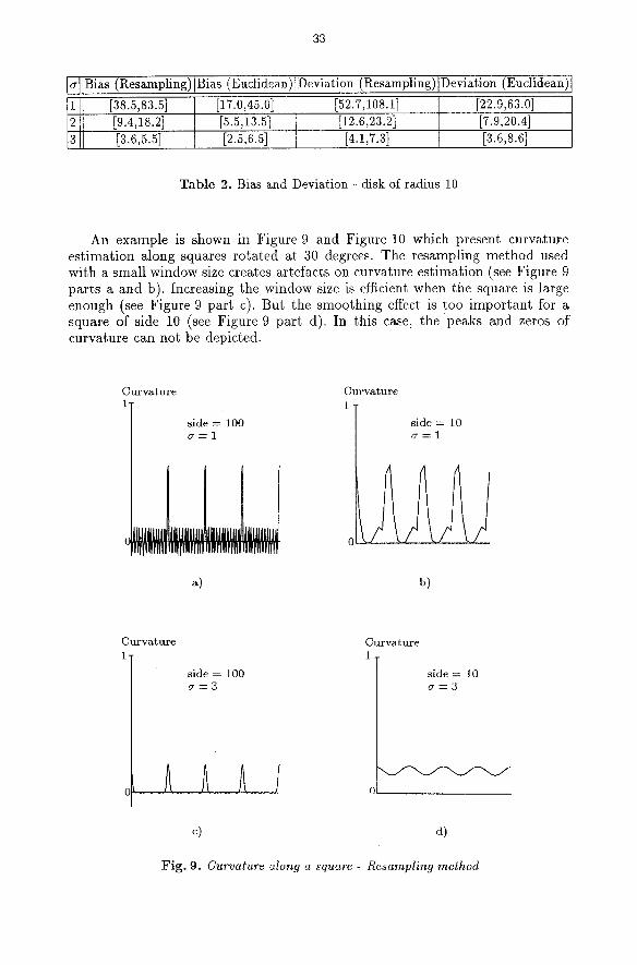
An example is shown in Figure 9 and Figure 10 which present curvature estimation along squares rotated at 30 degrees. The resampling method used with a small window size creates artefacts on curvature estimation (see Figure 9 parts a and b). Increasing the window size is efficient when the square is large enough (see Figure 9 part c). But the smoothing effect is too important for a square of side 10 (see Figure 9 part d). In this case, the peaks and zeros of curvature can not be depicted.

Curvature 1

side = 100 o . = l

~)

C u r v a t u r e

1

side -- 10 o . = 1

0

b)

Curvature 1-

side = 100 o ' = 3

o,A,,A A

Curvature 1

side = 10 o - = 3

c) d)

F i g . 9. Curvature along a square - R e s a m p l i n g me thod

34

On the contrary, the Euclidean method provides accurate results for both sizes of squares with ~ = 1 (see Figure 10). The previous remarks on squares are valid for any contour with non constant curvature and particularly for polygons.

C u r v a t u r e C u r v a t u r e

1" s i d e = 10

c r - ~ l

s i d e = 100

c r = l

Fig. 10. Curvature along a square - Euclidean path

5 C o n c l u s i o n

As the Euclidean boundary associated to a discrete object is a good reconstruc- tion of the underlying real boundary, it provides a correct estimation of perimeter and surface. The obtained results are at least as good as the ones obtained by classical methods. The most interesting property of the Euclidean method is that lenght estimation is little dependent on the position of the real object on the grid. Moreover the tangent estimation performed during the construction of Euclidean paths improves the curvature computation along a discrete path. The Euclidean model has also the advantage to be generic in the sense that it requires no interpretation of the discrete curve on the contrary of approaches such as vectorization.

These results have been presented in the 8-connected case which is the most used for geometrical parameter measurement. The 4-connected case is usually not taken into account which is directly related with the reduced number of different chain elements. Euclidean paths keep their qualities in this case. It is particularly interesting for analysing segmentation results defined as inter-pixels paths.

R e f e r e n c e s

1. J.P. Braquelaire and A. Vialard. Euclidean paths : a new representation of bound- ary of discrete regions. Technical Report 1088-95, LaBRI, UBX1, 1995. Submitted.

2. I. Debled and J.P. Reveilles. Un algorithme lin6aire de polygonalisation des courbes discr6tes. In Colloque Gdomdtrie discr4te en imagerie, pages 243-253, Grenoble, 1992.

35

3. L. Dorst and A.W. Smeulders. Lenght estimators for digitized contours. CVGIP, 40:311-333, 1987.

4. A. Vialard et J.P. Braquelaire. Transformations g~omdtriques de courbes discr~tes 2d. In 3~rnes journdes de I'AFIG (Marseille), 1995.

5. M. Kass, A. Witkin, and D. Terzopoulos. Snakes : active contour models. Int. Y. Comput. Vis., 4:321-331, 1987.

6. J.P. Reveilles. Gdorndtrie discrete, Calcul en nombres entiers et algorithmique. PhD thesis, Universit4 Louis Pasteur, Strasbourg, 1991.

7. A. Rosenfeld and A.C. Kak. Digital Picture Processing, volume 2. Academic Press, 1982.

8. B. Shahraray and D.J. Anderson. Uniform resampling of digitized contours. PAMI, 7(6):674-681, November 1985.

9. D. Terzopoulos, A. Platt , A. Barr, and K. Fleischer. Elastically deformable mod- els. Comput. Graph., 21:205-214, 1987.

10. A. Vialard. Les chemins euclidiens : module et applications. PhD thesis, Universit4 Bordeaux 1, 1996.

11. M. Worring and A. W.M. Smeulders. Digital curvature estimation. IU, 58(3):366- 382, November 1993.