Ser TH1 N2lr 2 no. 209 c. 2

ANALYZED NATIONAL RESEARCH COUNC IL

CANADA

D I V I S I O N OF BUILDING RESEARCH BLDG

THE CALCULATION OF SURFACE TEMPERATURE AND HEAT FLLJX

FROM SUBSURFACE TEMPERATURE MEASUREMENTS

BY

D. G. STEPHENSON AND G .P . MITALAS

( ~~~i~~~~~ t..;;ir.ii+ c ~ ~ i + c ~ ~

REPRINTED FROM i

TRANSACTIONS OF THE ENGINEERING INSTITUTE OF CANADA

VOL. 6 , NO. B-4, JULY 1963,

PAPER NO. E I C - 6 3 - M ~ c H 4

RESEARCH PAPER NO. 2 0 9

OF THE

D I V I S I O N OF BUILDING RESEARCH

P R I C E 50 CENTS

-! t-y yrr -) - - a u d l 3

OTTAWA

DECEMBER 1963

NRC 7 4 1 5

This publication is being distributed by the Division of Building Research of the National Research Council. It should not be reproduced in whole or in part, without permis- sion of the original publisher. The Division would be glad to be of assistance in obtaining such permission,

Publications of the Division of Building Research may be obtained by mailing the appropriate remittance, ( a Bank, Express, or Post Office Money Order or a cheque made payable at par in Ottawa, to the Receiver General of Canada, credit National Research Council) to the National Research Council, Ottawa. Stamps are not acceptable.

A coupon system has been introduced to make payments for publications relatively simple. Coupons are available in denominations of 5, 25 and 50 cents, and may be obtained by making a remittance as indicated above. These coupons may be used for the purchase of all National Research Council publi- cations including specifications of the Canadian Government Specifications Board.

THE CALCULATION OF SURFACE TEMPERATURE AND HEAT FLUX

FROM SUBSURFACE TEMPERATURE MEASUREMENTS

D. G. Stephenson and G. P. Mitalasq

SUMMARY

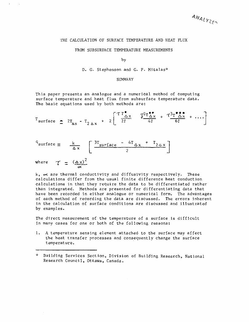
This paper presents an analogue and a numerical method of computing surface temperature and heat flux from subsurface temperature data. The basic equations used by both methods are:

ee . m e TAX + T A + ....I surface - - 2Tax - T2 A x + 2 4 ! 6!

lsurface = - W L T L surface A x 2

where = AX)^ rx

k, oc are thermal conductivity and diffusivity respectively. These calculations differ from the usual finite difference heat conduction calculations in that they require the data to be differentiated rather than integrated. Methods are presented for differentiating data that have been recorded in either analogue or numerical form. The advantages of each method of recording the data are discussed. The errors inherent in the calculation of surface conditions are discussed and illustrated by examples.

The direct measurement of the temperature of a surface is difficult in many cases for one or both of the following reasons:

1. A temperature sensing element attached to the surface may affect the heat transfer processes and consequently change the surface temperature.

Building Services Secti.on, Division of Building Research, National Research Council, Ottawa, Canada.

2. T h e r e may be some a c t i v i t y a t t h e s u r f a c e t h a t would q u i c k l y damage any thermometer .

Fo r example, a t he rmocoup le a t t a c h e d t o t h e o u t s i d e s u r f a c e o f a w a l l may have a d i f f e r e n t a b s o r p t i v i t y f o r s o l a r r a d i a t i o n from t h a t o f t h e w a l l s u r f a c e ; i t w i l l r e a c h a t e m p e r a t u r e d i f f e r e n t from t h a t o f t h e r e s t o f t h e w a l l s u r f a c e when s o l a r r a d i a t i o n i s a s i g n i f i c a n t t e r m i n t h e ene rgy b a l a n c e a t t h e s u r f a c e . A s e n s i n g e l emen t on a s u r f a c e c a n a l s o a l t e r t h e c o n v e c t i o n and l o n g wave r a d i a t i o n a t t h e s u r f a c e . The d i r e c t measurement o f t h e s u r f a c e t e m p e r a t u r e o f a n a s p h a l t pavement o r a c u l t i v a t e d f i e l d would b e d i f f i c u l t f o r t h e second r e a s o n . S u r f a c e p y r o m e t e r s a v o i d t h e s e d i f f i c u l t i e s b u t t h e y a r e u n a b l e t o d i s c r i m i n a t e be tween e m i t t e d a n d r e f l e c t e d r a d i a t i o n .

Approximate n u m e r i c a l methods h a v e been d e v e l o p e d r e c e n t l y f o r c a l - c u l a t i n g t h e s u r f a c e c o n d i t i o n s from measured v a l u e s a t p o i n t s below t h e s u r f a c e . S t o l z ( 1 ) c a l l s t h i s t h e s o l u t i o n o f a n i n v e r s e problem o f h e a t c o n d u c t i o n . Shumakov ( 2 ) h a s s t u d i e d t h e same problem and r e p o r t e d on i t i n t h e R u s s i a n l i t e r a t u r e . The p r e s e n t p a p e r p r e s e n t s a n o t h e r numer i ca l method t h a t h a s some a d v a n t a g e s o v e r t h o s e p r e v i o u s l y r e p o r t e d , and a n e l e c t r o n i c a n a l o g u e computer c i r c u i t t h a t is p a r t i c u l a r l y u s e f u l when s u r f a c e c o n d i t i o n s change r a p i d l y .

NUMERICAL METHODS OF CALCULATING SURFACE TEMPERATURE

The methods o f S t o l z and Shumakov a r e e s s e n t i a l l y t h e same: t h e y u s e t h e known r e l a t i o n s h i p be tween a u n i t p u l s e v a r i a t i o n o f t h e s u r f a c e t e m p e r a t u r e and t h e r e s u l t i n g change i n t h e t e m p e r a t u r e a t t h e d e p t h s where t h e t e m p e r a t u r e s a r e measured . The f o l l o w i n g d e r i v a t - i o n o f a fo rmula f o r To u s e s t h i s a p p r o a c h , b u t is i n t h e same t e r m i n - o l o g y as t h e r e s t o f t h i s p a p e r r a t h e r t h a n i n t h a t used by t h e o r i g i n a l a u t h a r s .

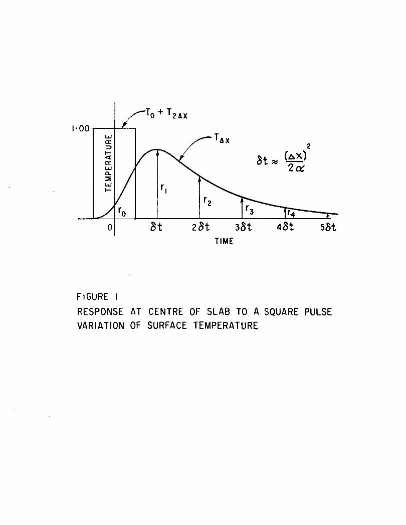
F i g u r e 1 shows t h e t e m p e r a t u r e r e s p o n s e a t t h e c e n t r e o f a s l a b , o f t h i c k n e s s 2 a x t h a t r e s u l t s f rom t h e s q u a r e p u l s e v a r i a t i o n o f t h e t e m p e r a t u r e a t t h e s u r f a c e s . The t e m p e r a t u r e To c a n be computed f rom t h e measured t e m p e r a t u r e s a t d e p t h s A x and 2 A x by t h e fo rmula .

where the factors r rl, r2, etc. are the ordinates of the response 0 curve shown in Fig. 1.

By rearranging, this becomes

Similarly

etc.

Thus

T r - 1

2 O,O - - - T 2 ~ x , ~ + I - T ~ ~ , ~ - AX, -6t + rl - q r O

r o r r T~x,-26t . . . . 2

0 0

This expression for the surface temperature uses the data at t < 0 but does not use the values at t > 0 that also have a strong correlation with To,o*

It is shown in Appendix A that the surface temperature is related to the subsurface temperatures T

and T2 AX by the following exact equation: A x

where (ax>L T =

- d T~~ - - (TAX) etc. dt

and oc - thermal diffusivity. -

The method of Stolz and Shumakov is equivalent to using backward difference approximations for the time derivatives of T in express-

A x ion A.

The following expression for To is based on central difference approx- imations for the time derivatives of TAX and consequently is more accurate than the Stolz or Shumakov formulae.

The coefficients a ... g are functions of the dimensionless number

The exact relationships are derived in Appendix B; and h = - 1.000. This equation takes account of all the differences of T up to the n x sixth, i.e. it approximates the first six derivatives of T a x and neglects all the higher differences. The first neglected term is

where A:n is the central seventh difference of T ax at time 0.

The error in the computed value of To is caused partly by neglecting the higher difference terms for TL\ x, and partly by errors in the measured values af T h x and T2nx. The maximum possible error caused by errors in the data is the possible error in any measured value times the sum of the absolute value of the coefficients a ... h. It is desirable, there- fore, to choose A x and 6t so that the coefficients are as small as possible, i.e. small values of A x and large values of bt. However, as 6t increases so do the difference terms and consequently the error associated with the neglected high order differences increases. Thus the optimum 6t from this point of view is a compromise that makes the total error a minimum.

The choice of 6t must also be based on the frequency spectrum of the data. It is well known in communications work that a sampled signal has an upper frequency limit of 112 6t. Thus, dt must be less than half the period of the highest frequency component that has to be considered.

I f t h e r e is h igh f requency n o i s e p r e s e n t i n t h e d a t a s i g n a l , t h e d a t a can be improved by averag ing . It is shown i n Appendix t h a t a n aver - ag ing ( i . e . i n t e g r a t i o n ) p roce s s a c t s a s a low pas s f i l t e r w i th t h e f a c t o r

F = S i n Y Y

where Y = (Averaging i n t e r v a l ) Cycle Pe r i od

F igu re 2 shows l og F a s o r d i n a t e and l o g (7 /n ) a s a b s c i s s a . For smal l va lue s of Y t h e f i l t e r f a c t o r i s e s s e n t i a l l y one, bu t w h e n y e q u a l s

X o r any whole number t imes n t h e f i l t e r f a c t o r is zero. The d o t t e d l i n e is t h e upper l i m i t of t h e f i l t e r f a c t o r i n t h e h igher f requency r eg ion .

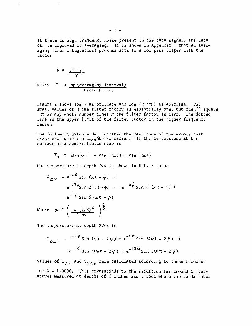
The fo l lowing example demons t ra tes t h e magnitude of t h e e r r o r s t h a t occur when M S ~ and wmax6t + 1 r ad i an . I f t h e t empera ture a t t h e s u r f a c e of a s e m i - i n f i n i t e s l a b is

To = S i n ( ~ , c t ) + S i n ( W ) + S i n ( 5 d )

t h e t empera ture a t dep th A x is shown i n Ref. 3 t o be

- 4 = e S i n ( ~ t - 4 ) +

e - 3 ' ~ i n 3 ( u t -4) + e -4 &

S i n 4 (G-t - $) + - 5 4..

e S i n 5 ( w t - ;/.)

m e r e c-$ = ( w ( A X ) ' )' 2 o<

The tempera ture a t dep th 2 A x is

-8 4 e S i n 4 ( w t - 2 6 ) + e - l 0 9 s i n 5 ( w t - 2 4 )

Values of Tax and T 2 A x

were c a l c u l a t e d acco rd ing t o t h e s e formulae'

f o r 4 = 1.0000. Th i s cor responds t o t h e s i t u a t i o n f o r ground temper- a t u r e s measured a t dep th s of 6 inches and 1 f o o t where t h e fundamental

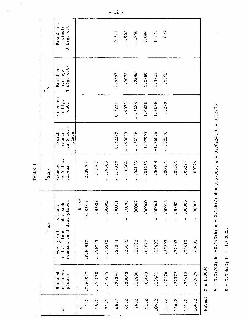
f requency is 1 c y c l e p e r day; o r f o r t e m p e r a t u r e s a t d e p t h s of 10 f e e t and 20 f e e t f o r a fundamental f r equency o f 1 c y c l e p e r y e a r . These v a l u e s were used t o compute To by e q u a t i o n A and t h e r e s u l t i n g v a l u e s a r e compared i n T a b l e I w i t h t h e e x a c t v a l u e s o b t a i n e d by e v a l u a t i n g t h e i n i t i a l s i n e s e r i e s .

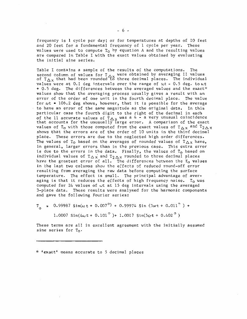
Table I c o n t a i n s a sample of t h e r e s u l t s of t h e computat ions . The second column of v a l u e s f o r T ~ , were o b t a i n e d by a v e r a g i n g 11 v a l u e s o f T A ~ t h a t had been rounded t o t h r e e decimal p l a c e s . The i n d i v i d u a l v a l u e s were a t 0.1 deg i n t e r v a l s o v e r t h e r a n g e of c ~ t - 0 .5 deg. t o w t + 0 .5 deg. The d i f f e r e n c e s between t h e averaged v a l u e s and t h e exact:k v a l u e s show t h a t t h e a v e r a g i n g p r o c e s s u s u a l l y g i v e s a r e s u l t w i t h a n e r r o r of t h e o r d e r o f one u n i t i n t h e f o u r t h decimal p l a c e . The v a l u e f o r w t - 106.2 deg shows, however, t h a t i t is p o s s i b l e f o r t h e a v e r a g e t o have a n e r r o r of t h e same magni tude a s t h e o r i g i n a l d a t a . I n t h i s p a r t i c u l a r c a s e t h e f o u r t h d i g i t t o t h e r i g h t of t h e decimal i n each o f t h e 11 a c c u r a t e v a l u e s o f TA, was a 4 - a v e r y unusual c o i n c i d e n c e t h a t a c c o u n t s f o r t h e u n u s u a l l y l a r g e e r r o r . A comparison of t h e e x a c t v a l u e s o f To w i t h t h o s e computed from t h e e x a c t v a l u e s of T A X and T z A x shows t h a t t h e e r r o r s a r e of t h e o r d e r o f 1 0 u n i t s i n t h e t h i r d decimal p l a c e . These e r r o r s a r e due t o t h e n e g l e c t e d h i g h o r d e r d i f f e r e n c e s . The v a l u e s o f To based on t h e a v e r a g e s of rounded v a l u e s of T a x have, i n g e n e r a l , l a r g e r e r r o r s t h a n i n t h e p r e v i o u s case . Th i s e x t r a e r r o r i s due t o t h e e r r o r s i n t h e d a t a . F i n a l l y , t h e v a l u e s o f To based on i n d i v i d u a l v a l u e s of T A k and T2A, rounded t o t h r e e decimal p l a c e s have t h e g r e a t e s t e r r o r of a l l . The d i f f e r e n c e s b e t w e m t h e ro v a l u e s i n t h e l a s t two columns shot7 t h e e f f e c t s 3f reduced round-off e r r o r r e s u l t i n g from a v e r a g i n g t h e raw d a t a b e f o r e computing t h e s u r f a c e t empera tu re . The e f f e c t is smal l . The p r i n c i p a l advan tage of a v e r - a g i n g is t h a t i t r e d u c e s t h e e f f e c t s of h i g h f requency n o i s e . To was computed f o r 24 v a l u e s of ~ - t a t 1 5 deg i n t e r v a l s u s i n g t h e averaged 3 - p l a c e d a t a . These r e s u l t s were a n a l y s e d f o r t h e harmonic components and gave t h e f o l l o w i n g F o u r i e r s e r i e s :

To = 0.99987 Sin(.wt + 0.007") + 0.99974 S i n ( 3 w t + 0.011" ) +

These t e rms a r e a l l i n e x c e l l e n t agreement w i t h t h e i n i t i a l l y assumed s i n e s e r i e s f o r To.

* ' e x a c t ' means a c c u r a t e t o 5 decimal p l a c e s

AN ANALOGUE METHOD OF COMPUTING SURFACE TEMPERATURE

An analogue computer can be used to compute To if the temperature at depths A x and 2 A x are available as continuous electrical signals. A computer could be operated at real time with the data supplied directly from the measuring equipment. In some cases it may be more practical, however, to record TAX T2nx and subsequently play them back as the input to a computer. If the recorder has a range of record and play back speeds the time scale of the computer need not be the same as the time scale of the original experiment.

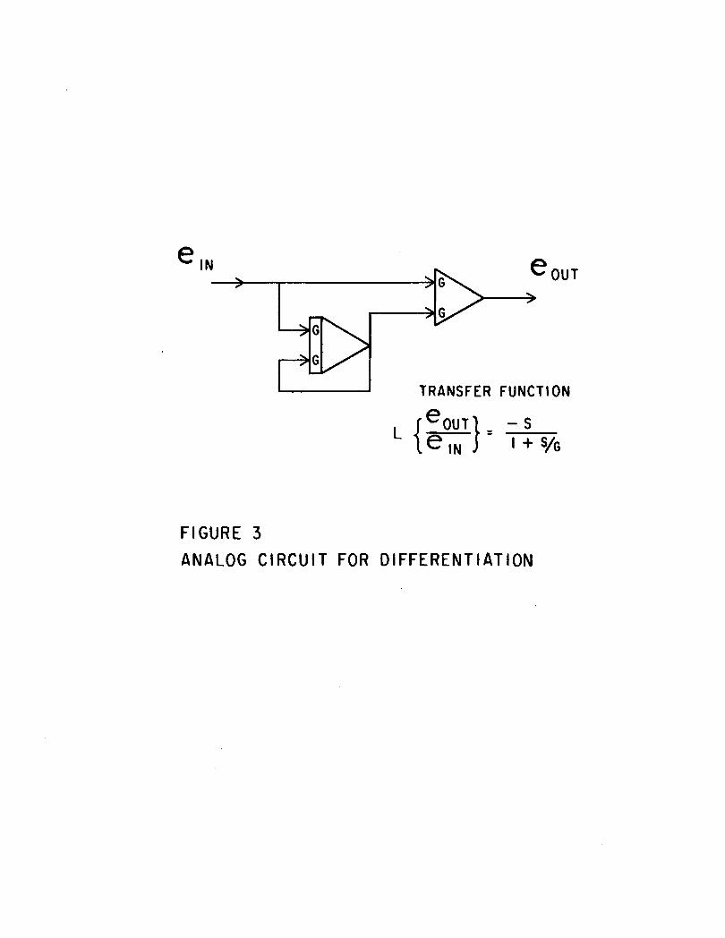
The basic equation for an analogue computation is the same as for the digital, i.e. equation A. The difficulty in using this equation comes from the differentiation of TA, . The circuit shown in Fig. 3 has the transfer function

whereas an ideal differentiator would be simply s. The output of this circuit is a good approximation of the time derivative of the input for low frequencies, but the approximation gets progressively worse as the frequency increases.

The Laplace transformation of equation A is

1 = cosh (fs) 2

2! 4! 6!

The computer circuit shown in Fig. 4 has a transfer function

1 - ( T 0 2 + T ~ ~ X ) that approximates cosh (7s) 2 . The frequency

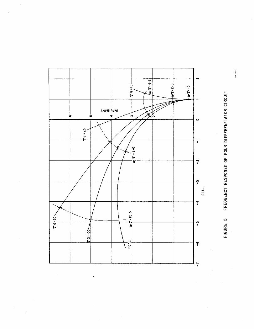
response diagram for the analogue circuit is shown in Fig. 5. The transfer function is a better approximation for cosh (Ts) 1 the

7 larger the value of GT. Unfortunately, the signal to noise ratio is reduced by the factor L- /G at each differentiation so that the choice of G must be a compromise between transfer function accuracy and noise.

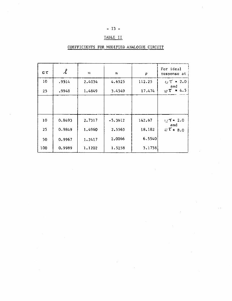
Figure 6 shows the contribution to the final output of each different- iator unit for WT = 8 radians and GT = 25. The vector OP represents the ideal frequency response, C O S ~ ( iwT) $- ; and the vector OQ

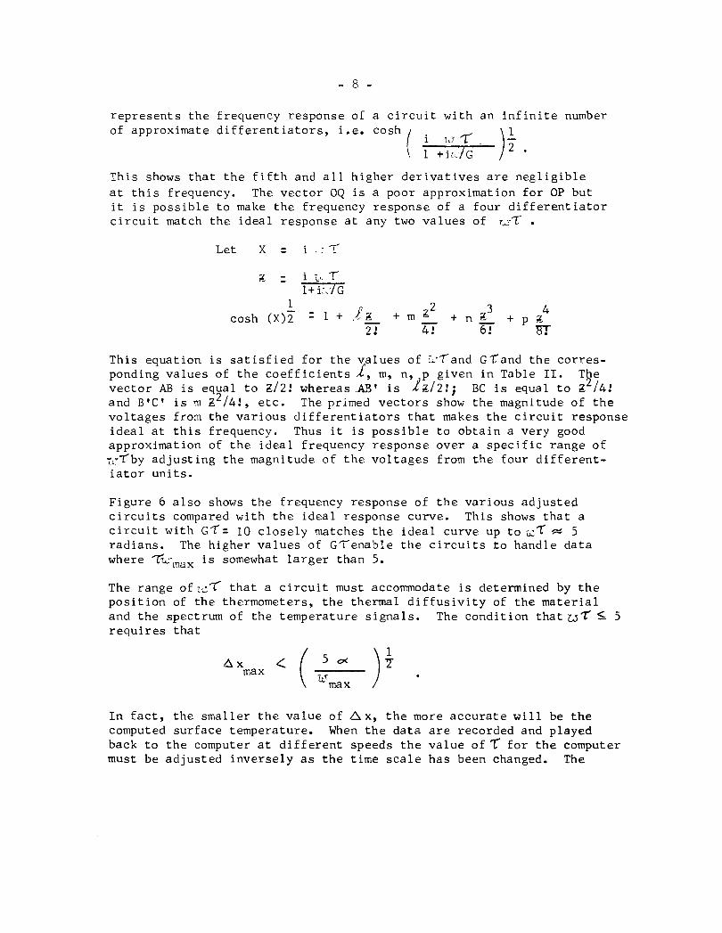
represents the frequency response of a circuit with an infinite number of approximate differentiators, i.e. cosh

i r,r I , 1 + i .:::/G )+ .

This shows that the fifth and all higher derivatives are negligible at this frequency. The vector OQ is a poor approximation for OP but it is possible to make the frequency response of a four differentiator circuit match the ideal response at any two values of 7 ~ - 7 .

Let X = i.:?

This equation is satisfied for the values of iiryand Grand the corres- ponding values of the coefficients 1, m, n, p given in Table 11. The vector AB is equal to Z/Z! whereas A B t is IZ/Z!; BC is equal to g2/4! and B t C t is m z2/4!, etc. The primed vectors show the magnitude of the voltages from the various differentiators that makes the circuit response ideal at this frequency. Thus it is possible to obtain a very good approximation of the ideal frequency response over a specific range of ;,:Thy adjusting the magnitude of the voltages from the four different- iator units.

Figure 6 also shows the frequency response of the various adjusted circuits compared with the ideal response curve. This shows that a circuit with GT= 10 closely matches the ideal curve up to cr c-- 5 radians. The higher values of GTenable the circuits to handle data where TcmaX is somewhat larger than 5.

The range ofzsT that a circuit must accommodate is determined by the position of the thermometers, the thermal diffusivity of the material and the spectrum of the temperature signals. The condition t h a t ~ T 5 5 requires that

In fact, the smaller the value of A x , the more accurate will be the computed surface temperature. When the data are recorded and played back to the computer at different speeds the value o f r for the computer must be adjusted inversely as the time scale has been changed. The

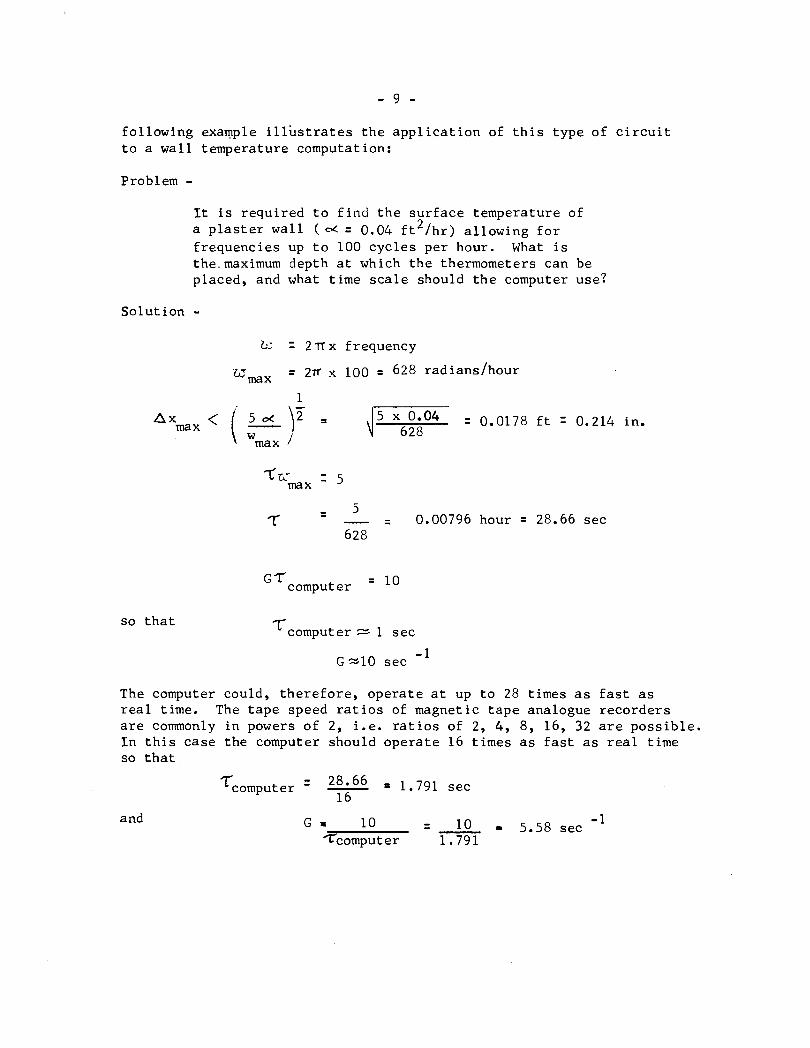
following example illustrates the application of this type of circuit to a wall temperature computation:

Problem - It is required to find the surface temperature of a plaster wall ( d = 0.04 ft2/hr) allowing for frequencies up to 100 cycles per hour. What is the.maximum depth at which the thermometers can be placed, and what time scale should the computer use?

Solution - L: = 2TT x frequency

umax = 2n 100 = 628 radianslhour

1

A x m x < ( i d \T = 0°04 = 0.0178 ft = 0.214 in. W max

\I 628

Tc max 5

= 5 7 - = 0.00796 hour = 28.66 sec

628

G T computer = 10

so that Zcomput er i 1 sec

- 1 G ~ 1 0 sec

The computer could, therefore, operate at up to 28 times as fast as real time. The tape speed ratios of magnetic tape analogue recorders are commonly in powers of 2, i.e. ratios of 2, 4, 8, 16, 32 are possible. In this case the computer should operate 16 times as fast as real time so that

- 28.66 Tcomputer - - = 1.791 sec 16

and

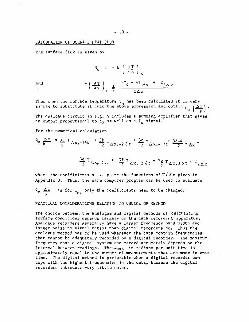
CALCULATION OF SURFACE HEAT FLUX

The surface flux is given by

and - / L i z \ . 3T0 - 4T Ax + T 2 ~ x

Thus when the surface temperature T has been calculated it is very 0

simple to substitute it into the above expression and obtain AX . qo [ T I

The analogue circuit in Fig. 4 includes a summing amplifier that gives an output proportional to qo as well as a To signal.

For the numerical calculation

where the coefficients a ... g are the functions of^/ 6 t given in Appendix B. Thus, the same computer program can be used to evaluate

A x as for To. only the coefficients need to be changed. qo - k 9

PRACTICAL CONSIDERATIONS RELATING TO CHOICE OF METHOD

The choice between the analogue and digital methods of calculating surface conditions depends largely on the data recording apparatus. Analogue recorders generally have a larger frequency band width and larger noise to signal ratios than digital recorders do. Thus the analogue method has to be used whenever the data contain frequencies that cannot be adequately recorded by a digital recorder. The maximum frequency that a digital system can record accurately depends on the interval between readings. TheV~:rnax in radians per unit time is approximately equal to the number of measurements that are made in unit time. The digital method is preferable when a digital recorder can cope with the highest frequencies in the data, because the digital recorders introduce very little noise.

CONCLUSION

The temperature and heat flux at the surface of a slab of homogeneous material can be computed from measured values of the temperature at two known depths below the surface and the values of thermal conductiv- ity and diffusi-~ity of the material. The accuracy of the computed surface conditions depends on the depth at which the temperatures are measured; the accuracy is best when the thermometers are close to the surface.

The computation can be made with an analogue computer or by an all- numerical technique that is suitable for programming on a digital computer. It has been shown that the numerical technique is satis- factory for values of 6t =7/2 andXmaxT 5 2 radians. No other values of these parameters were tested. The analogue method has been shown to be accurate from UmxTup to 5 radians for Gf= 10 and the unusable band width can be increased by increasing the value of GTand accept- ing higher noise to signal ratios.

REFERENCES

1. Stolz, G., Numerical Solutions to an Inverse Problem of Heat Conduction for Simple Shapes. ASME Journal of Heat Transfer, Vol. 82, Series C, No. 1, Feb. 1960, p. 20.

2. Shumakov, N.V., A Method for the Experimental Study of the Process of Heating a Solid Body. Soviet Physics - Technical Physics (translated by American Institute of physics), Vol. 2, 1957, p. 771.

3. Carslaw, H.S., and Jaeger, J.C., Conduction of Heat in Solids. Oxford Press, 1959, p. 65.

This paper is a contribution from the Division of Building Research, National Research Council, and is published with the approval of the Director of the Division.

I 4

W

Fd u r-'

N 0 m o d m - 9 0 4 0 m o o . . .

0 r-'

X ' m

a N

r-'

X a

r-'

c m O a J U

4 m M'm

.a c aJ .,-4 . VJ VJ M m .,-4

m w I

m

m c U 0 a J m

M V '-0 m aJk VJ aJ M

!a $ 2 m

c 0 '

M m '0 '4 U ( U W m VJ I ' m m In m

'-0 0 UaJaJaJ u'm'm u ( d ~ m X 3 I n d w o a

k 0 U

0 'm aJ aJ'm VJ

aJ

~ j ~ : 0 0 d ~ ' u a

VJ J= a

m u 0 a J m m 3 a J d 4 a m vl 3 U

c G F i a J a J

d g " m W k m 0 U

c 0 aJ .d u M m o -o k d aJ aJ . 'm 3 0 C

u L ) g m k

-

'0 U a J a J V J -0-0 aJ

0

3 m 5 0 ,z o a

L)

d N S d r C l b N O I n m b N I n m c u o m m

0 d d I I

r - N d m m m I n r - m m 0 9

r- N : g 2 & m m

0 d d I I

- ~ m w m a o I n b W N b b N 0 3 9 N I n g 2 o m m

0 d d I I

I n m 9 I n 9 N m r - - m 2 - N O d m O I n N 0 b 9 N I n m Z o m m

0 d d I I + + +

N h 9 0 3 d r C I r C 1 0 3 9 a I n O N I n m ~ s E 2 N S m o m m m m - : 2 g g ; ; t s N g O ~ ~ ~ ~ O O O O O O O

0 I I I I I I I I

k o r - - m ~ m - o d m c n m d k d O O d O O O d d 0 0 0 k O O O O O O O O O O O O w 0 0 0 0 0 0 0 0 0 0 0 0

0 0 0 0 0 0 0 0 0 0 0 0

0 I I I I I I +

0 m o m o m m o m m m m d N m m d m d o a a d m m O I n N C O m m d N h 9 d m 9 0 - 0 ~ m m - ~ d 0 a m d ~ m d ~ d ~ m m d . 0 I I I

- 0 I n d m 9 m d 9 N m O ~ m ~ m d m d d - - d h m O I n N C O m a ) N - a d m \ b O + O N C ? s - 0 a I n d N m d o d N Z S d

o I I I

N N N N N N N N N N N N . . d 9 d a d 9 d 9 d a d a

u 3

-

o d m d a t - m o ~ m m 9 d d d d d

- 13 - TABLE I1

C O E F F I C I E X T S FOR M O D I F I E D ANALOGUE C I R C U I T

G Z

10

2 5

10

2 5

50

100

R .9514

.9948

0.8493

0.9849

0.9967

0.9989

! i ' For i d e a l ! response a t i

---1: 111 n

2.4034

1.4849

2.7317

1.4960

1.2417

1.1202

~ , 7 ' = 2.01 and 1

W Z 4.5 ] -- -- - -J

i

i .?*T- .-,. 2.0

l,i'sc= 8.0

and 1

4.6525 1 112.25 ' 3.4549

-5.3612

2.5563

2.0066

1.5258

17.474

142.67

18.182

6.5540

3.1738

THE CALCULATION OF SURFACE TEMPERATURE AND HEAT FLUX

FROM SUBSURFACE TEMPERATURE MEASUREMENTS

by

D. G. Stephenson and G. P. Mitalas

FIGURE CAPTIONS

Figure 1 Response at centre of slab to a square pulse variation of surface temperature

Figure 2 Frequency response of numerical filter that averages data over an interval of 2 Z

Figure 3 Analogue circuit for differentiation

Figure 4 Analogue circuit to compute surface temperature and heat f 1 ux

Figure 5 Frequency response of four-differentiator circuit

Figure 6 Frequency response of modified four-differentiator circuits

W a 3 2 l- a a W

(ax)

r l

f

o 6 t 26t 3 S t 4 8 t 56t TIME

FIGURE I

RESPONSE AT CENTRE OF SLAB TO A SQUARE PULSE VARIATION OF SURFACE TEMPERATURE

oao w m e . . . . . CU -

- TRANSFER FUNCTI

OUT

ON

FIGURE 3

ANALOG CIRCUIT FOR DIFFERENTIATION

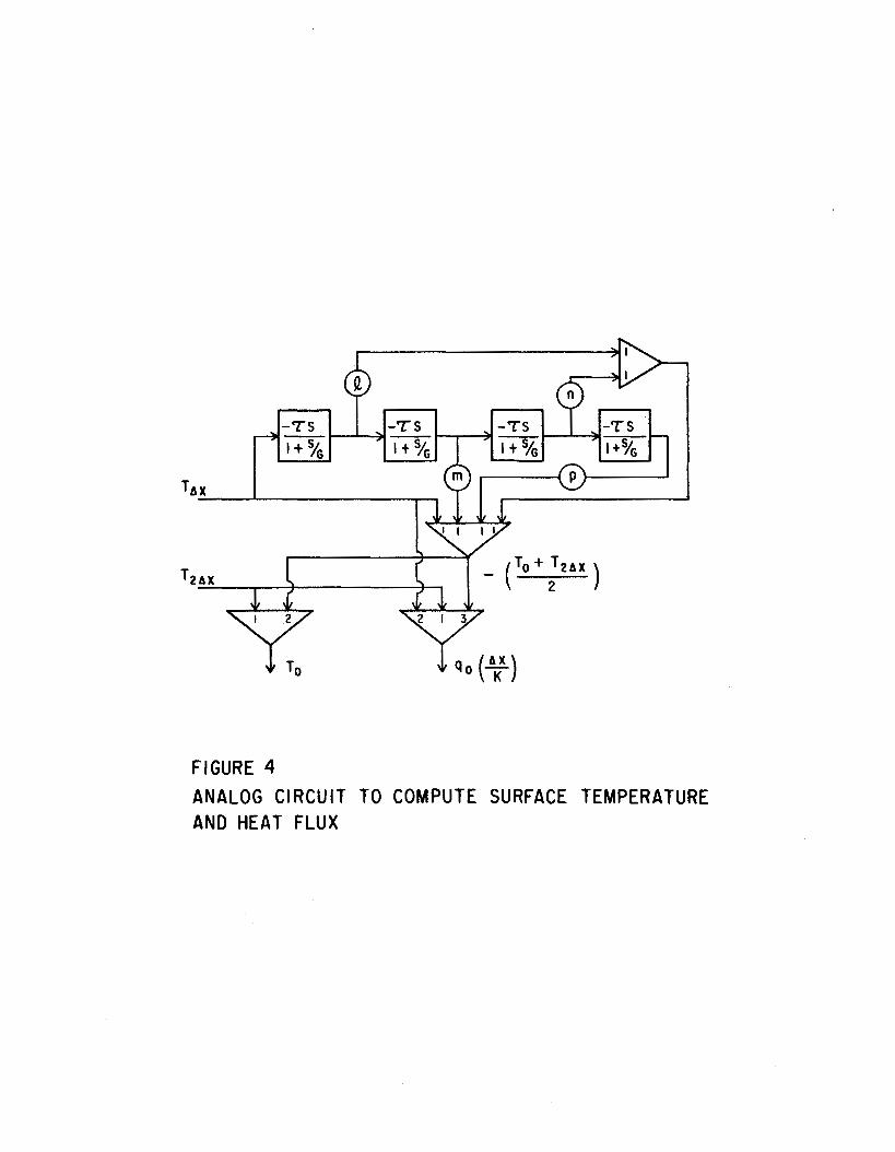
FIGURE 4 ANALOG CIRCUIT TO COMPUTE SURFACE TEMPERATURE AND HEAT FLUX

T G = I O FITTED AT 6,2= 2 AND (JZ= 4.5 2 G= 25 FITTED AT (LIZ ' 2 AND U Z = 4.5

- 7 - 6 - 5 - 4 - 3 - 2 -I 0 I 2

REAL

FIGURE 6 FREQUENCY RESPONSE OF MODIFIED FOUR DIFFERENTIATOR CIRCUITS

80 2MJ-I

APPENDIX A

Relationship between surface temperature and

subsurface temperatures

Let the temperature at the surface of a semi-infinite slab be To; at a depthax be T A X and at a depth 2 A x be T2nx. The temperature every- where in the material is described by

3T - d2, - at - bx'

where o(= thermal diffusivity.

The Laplace transform of this equation gives

where Q = Lrne-" . T dt . The initial conditions have been assumed to be

This simplifies the solution without any loss of generality since the solution of interest in this case is the one that depends on the boundary condition rather than the initial condition.

The solution of this simple second order differential equation is

2 Let 3 = 2

(ax) = Is d

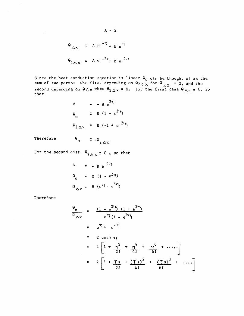
S i n c e t h e h e a t conduc t ion e q u a t i o n is l i n e a r Q0 c a n be though t of a s t h e sum of two p a r t s : t h e f i r s t depending on Q2p-x f o r Q, ,x -- = 0 , and t h e second depending on 8~~ when Q 2 A x = 0 . For t h e f i r s t c a s e Q A x = 0 , s o t h a t

A = - B e 2rl

Q = B ( 1 - e 291 )

0

O z A x = B ( -1 + e 2.'')

T h e r e f o r e

For t h e second c a s e 0 2 A x = 0 , so t h a t

T h e r e f o r e

= 2 cosh 7

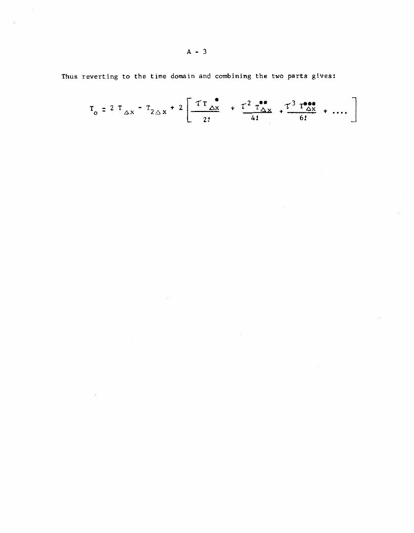
Thus reverting to the time domain and combining the two parts gives:

APPENDIX B

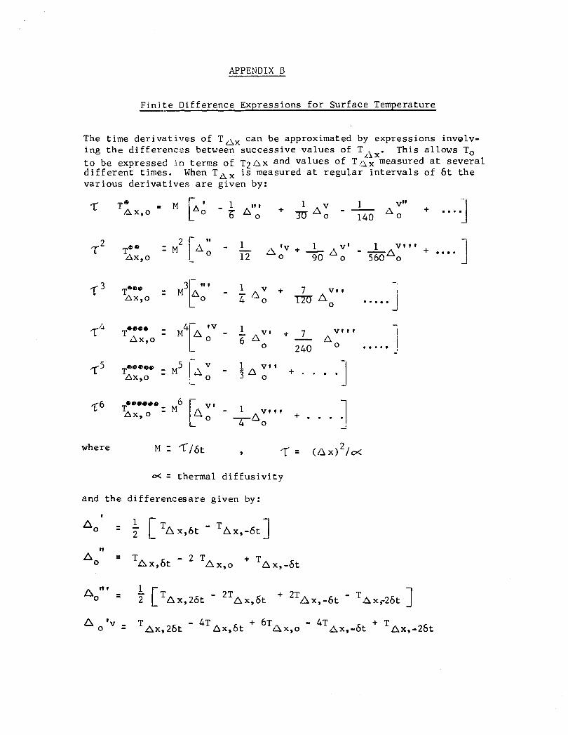
Finite Difference Expressions for Surface Temperature -

The time derivati ing the dif f erenc to be expressed i different times.

ves of TAX can be approximated by expressions involv- :cs between successive values of T A x- This allows To

terms of T ~ A ~ and values of T,&, measured at several When T A X is measured at regular intervals of 6t the

various derivatives are given by:

where M = </tit 9 2 T = (AX) /o(

d = thermal diffusivity

and the differencesare given by:

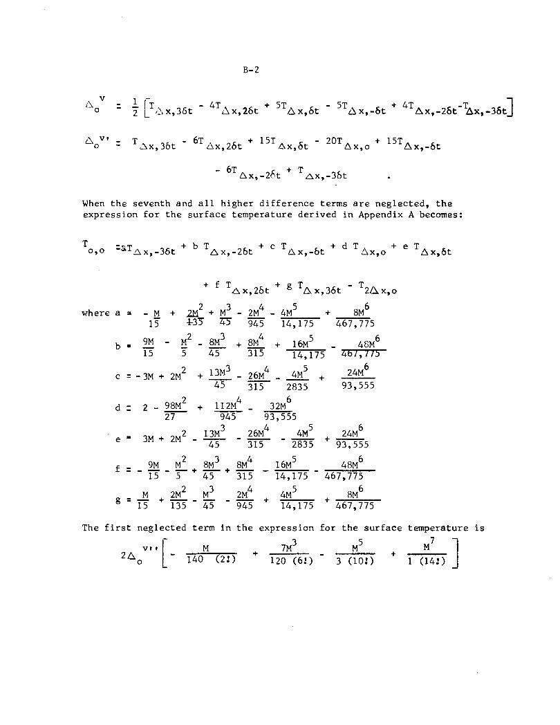
When the seventh and all higher difference terms are neglected, the expression for the surface temperature derived in Appendix A becomes:

2 where a a - M + 2C1 + M3 - 2M4 - 4M 5 + 8M 6 -

15 43'5 945 14,175 467,775

The first neglected term in the expression for the surface temperature is

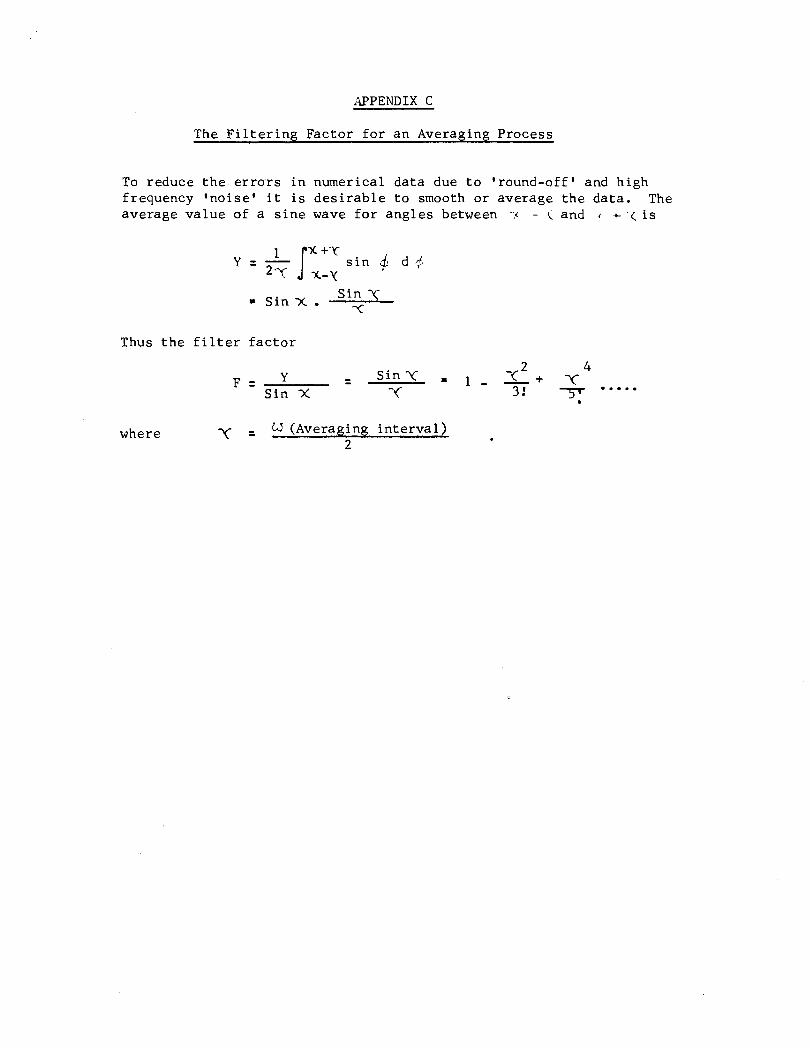
The F i l t e r i n g F a c t o r f o r a n Averaging P r o c e s s

To reduce t h e . e r r o r s i n numerical d a t a due t o ' round-of f ' and h igh f requency ' n o i s e ' i t is d e s i r a b l e t o smooth o r a v e r a g e t h e d a t a . The a v e r a g e v a l u e o f a s i n e wave f o r a n g l e s between - C and ( + .( is

1 X +'Y Y=-1 s i n 4 d d 2-u: x-y

S i n Y - S i n X . Thus t h e f i l t e r f a c t o r

- S i n Y -< 4 F = - = 1 - + Y

S i n X Y 3: =.... . where y = (Averaging i n t e r v a l )

2