arX

iv:1

701.

0077

6v2

[m

ath-

ph]

8 J

an 2

018

Analytical Methods in Physics

Yi-Zen Chu

Contents

1 Preface 4

2 Complex Numbers and Functions 7

3 Matrix Algebra: A Review 123.1 Basics, Matrix Operations, and Special types of matrices . . . . . . . . . . . . . 123.2 Determinants, Linear (In)dependence, Inverses and Eigensystems . . . . . . . . 153.3 Special Topic 1: 2D real orthogonal matrices . . . . . . . . . . . . . . . . . . . . 23

4 Linear Algebra 264.1 Definition . . . . . . . . . . . . . . . . . . . . . . . . . . . . . . . . . . . . . . . 264.2 Inner Products . . . . . . . . . . . . . . . . . . . . . . . . . . . . . . . . . . . . 294.3 Linear Operators . . . . . . . . . . . . . . . . . . . . . . . . . . . . . . . . . . . 35

4.3.1 Definitions and Fundamental Concepts . . . . . . . . . . . . . . . . . . . 354.3.2 Hermitian Operators . . . . . . . . . . . . . . . . . . . . . . . . . . . . . 404.3.3 Unitary Operation as Change of Orthonormal Basis . . . . . . . . . . . . 48

4.4 Tensor Products of Vector Spaces . . . . . . . . . . . . . . . . . . . . . . . . . . 564.5 Continuous Spaces and Infinite D−Space . . . . . . . . . . . . . . . . . . . . . . 58

4.5.1 Preliminaries: Dirac’s δ and eigenket integrals . . . . . . . . . . . . . . . 584.5.2 Continuous Operators, Translations, and the Fourier transform . . . . . . 614.5.3 Boundary Conditions, Finite Box, Periodic functions and the Fourier Series 72

5 Calculus on the Complex Plane 755.1 Differentiation . . . . . . . . . . . . . . . . . . . . . . . . . . . . . . . . . . . . . 755.2 Cauchy’s integral theorems, Laurent Series, Analytic Continuation . . . . . . . . 795.3 Poles and Residues . . . . . . . . . . . . . . . . . . . . . . . . . . . . . . . . . . 875.4 Branch Points, Branch Cuts . . . . . . . . . . . . . . . . . . . . . . . . . . . . . 945.5 Fourier Transforms . . . . . . . . . . . . . . . . . . . . . . . . . . . . . . . . . . 99

5.5.1 Application: Damped Driven Simple Harmonic Oscillator . . . . . . . . . 1015.6 Fourier Series . . . . . . . . . . . . . . . . . . . . . . . . . . . . . . . . . . . . . 105

1

6 Advanced Calculus: Special Techniques and Asymptotic Expansions 1076.1 Gaussian integrals . . . . . . . . . . . . . . . . . . . . . . . . . . . . . . . . . . . 1076.2 Complexification . . . . . . . . . . . . . . . . . . . . . . . . . . . . . . . . . . . 1096.3 Differentiation under the integral sign (Leibniz’s theorem) . . . . . . . . . . . . 1096.4 Symmetry . . . . . . . . . . . . . . . . . . . . . . . . . . . . . . . . . . . . . . . 1116.5 Asymptotic expansion of integrals . . . . . . . . . . . . . . . . . . . . . . . . . . 113

6.5.1 Integration-by-parts (IBP) . . . . . . . . . . . . . . . . . . . . . . . . . . 1146.5.2 Laplace’s Method, Method of Stationary Phase, Steepest Descent . . . . 115

6.6 JWKB solution to −ǫ2ψ′′(x) + U(x)ψ(x) = 0, for 0 < ǫ≪ 1 . . . . . . . . . . . . 122

7 Differential Geometry of Curved Spaces 1247.1 Preliminaries, Tangent Vectors, Metric, and Curvature . . . . . . . . . . . . . . 1247.2 Locally Flat Coordinates & Symmetries, Infinitesimal Volumes, General Tensors,

Orthonormal Basis . . . . . . . . . . . . . . . . . . . . . . . . . . . . . . . . . . 1297.3 Covariant derivatives, Parallel Transport, Levi-Civita, Hodge Dual . . . . . . . . 1417.4 Hypersurfaces . . . . . . . . . . . . . . . . . . . . . . . . . . . . . . . . . . . . . 161

7.4.1 Induced Metrics . . . . . . . . . . . . . . . . . . . . . . . . . . . . . . . . 1617.4.2 Fluxes, Gauss-Stokes’ theorems, Poincare lemma . . . . . . . . . . . . . . 164

8 Differential Geometry In Curved Spacetimes 1748.1 Poincare and Lorentz symmetry . . . . . . . . . . . . . . . . . . . . . . . . . . . 1748.2 Constancy of c; Orthonormal Frames; Timelike, Spacelike vs. Null Vectors; Grav-

itational Time Dilation . . . . . . . . . . . . . . . . . . . . . . . . . . . . . . . . 1838.3 Connections, Curvature, Geodesics, Isometries . . . . . . . . . . . . . . . . . . . 1918.4 Equivalence Principles & Geometry-Induced Tidal Forces . . . . . . . . . . . . . 2028.5 Special Topic 1: Gravitational Perturbation Theory . . . . . . . . . . . . . . . . 2128.6 Special Topic 2: Conformal/Weyl Transformations . . . . . . . . . . . . . . . . . 217

9 Linear Partial Differential Equations (PDEs) 2209.1 Laplacians and Poisson’s Equation . . . . . . . . . . . . . . . . . . . . . . . . . 220

9.1.1 Poisson’s equation, uniqueness of solutions . . . . . . . . . . . . . . . . . 2209.1.2 (Negative) Laplacian as a Hermitian operator . . . . . . . . . . . . . . . 2219.1.3 Inverse of the negative Laplacian: Green’s function and reciprocity . . . 2239.1.4 Kirchhoff integral theorem and Dirichlet boundary conditions . . . . . . 226

9.2 Laplacians and their spectra . . . . . . . . . . . . . . . . . . . . . . . . . . . . . 2299.2.1 Infinite RD in Cartesian coordinates . . . . . . . . . . . . . . . . . . . . . 2299.2.2 1 Dimension . . . . . . . . . . . . . . . . . . . . . . . . . . . . . . . . . . 2309.2.3 2 Dimensions . . . . . . . . . . . . . . . . . . . . . . . . . . . . . . . . . 2329.2.4 3 Dimensions . . . . . . . . . . . . . . . . . . . . . . . . . . . . . . . . . 239

9.3 Heat/Diffusion Equation . . . . . . . . . . . . . . . . . . . . . . . . . . . . . . . 2429.3.1 Definition, uniqueness of solutions . . . . . . . . . . . . . . . . . . . . . . 2429.3.2 Heat Kernel, Solutions with ψ(∂D) = 0 . . . . . . . . . . . . . . . . . . . 2449.3.3 Green’s functions and initial value formulation in a finite domain . . . . 2479.3.4 Problems . . . . . . . . . . . . . . . . . . . . . . . . . . . . . . . . . . . 248

9.4 Massless Scalar Wave Equation (Mostly) In Flat Spacetime RD,1 . . . . . . . . . 250

2

9.4.1 Spacetime metric, uniqueness of Minkowski wave solutions . . . . . . . . 2509.4.2 Waves, Initial value problem, Green’s Functions . . . . . . . . . . . . . . 2559.4.3 4D frequency space, Static limit, Discontinuous first derivatives . . . . . 2719.4.4 Initial value problem via Kirchhoff representation . . . . . . . . . . . . . 277

9.5 Variational Principle in Field Theory . . . . . . . . . . . . . . . . . . . . . . . . 2799.6 Appendix to linear PDEs discourse:

Symmetric Green’s Function of a real 2nd Order ODE . . . . . . . . . . . . . . 281

A Copyleft 287

B Conventions 288

C Physical Constants and Dimensional Analysis 289

D Acknowledgments 291

E Last update: January 9, 2018 291

3

1 Preface

This work constitutes the free textbook project I initiated towards the end of Summer 2015,while preparing for the Fall 2015 Analytical Methods in Physics course I taught to upper level(mostly 2nd and 3rd year) undergraduates here at the University of Minnesota Duluth. DuringFall 2017, I taught the graduate-level Differential Geometry and Physics in Curved Spacetimeshere at National Central University, Taiwan; this has allowed me to further expand the text.

I assumed that the reader has taken the first three semesters of calculus, i.e., up to multi-variable calculus, as well as a first course in Linear Algebra and ordinary differential equations.(These are typical prerequisites for the Physics major within the US college curriculum.) Myprimary goal was to impart a good working knowledge of the mathematical tools that underliefundamental physics – quantum mechanics and electromagnetism, in particular. This meant thatLinear Algebra in its abstract formulation had to take a central role in these notes.1 To this end,I first reviewed complex numbers and matrix algebra. The middle chapters cover calculus beyondthe first three semesters: complex analysis and special/approximation/asymptotic methods. Thelatter, I feel, is not taught widely enough in the undergraduate setting. The final chapter is meantto give a solid introduction to the topic of linear partial differential equations (PDEs), whichis crucial to the study of electromagnetism, linearized gravitation and quantum mechanics/fieldtheory. But before tackling PDEs, I feel that having a good grounding in the basic elements ofdifferential geometry not only helps streamlines one’s fluency in multi-variable calculus; it alsoprovides a stepping stone to the discussion of curved spacetime wave equations.

Some of the other distinctive features of this free textbook project are as follows.Index notation and Einstein summation convention is widely used throughout the physics

literature, so I have not shied away from introducing it early on, starting in §(3) on matrixalgebra. In a similar spirit, I have phrased the abstract formulation of Linear Algebra in §(4)entirely in terms of P.A.M. Dirac’s bra-ket notation. When discussing inner products, I do makea brief comparison of Dirac’s notation against the one commonly found in math textbooks.

I made no pretense at making the material mathematically rigorous, but I strived to makethe flow coherent, so that the reader comes away with a firm conceptual grasp of the overallstructure of each major topic. For instance, while the full fledged study of continuous (as opposedto discrete) vector spaces can take up a whole math class of its own, I feel the physicist shouldbe exposed to it right after learning the discrete case. For, the basics are not only accessible, theFourier transform is in fact a physically important application of the continuous space spanned bythe position eigenkets |~x〉. One key difference between Hermitian operators in discrete versuscontinuous vector spaces is the need to impose appropriate boundary conditions in the latter;this is highlighted in the Linear Algebra chapter as a prelude to the PDE chapter §(9), wherethe Laplacian and its spectrum plays a significant role. Additionally, while the Linear Algebrachapter was heavily inspired by the first chapter of Sakurai’s Modern Quantum Mechanics, Ihave taken effort to emphasize that quantum mechanics is merely a very important applicationof the framework; for e.g., even the famous commutation relation [X i, Pj ] = iδij is not necessarilya quantum mechanical statement. This emphasis is based on the belief that the power of a given

1That the textbook originally assigned for this course relegated the axioms of Linear Algebra towards thevery end of the discussion was one major reason why I decided to write these notes. This same book also costnearly two hundred (US) dollars – a fine example of exorbitant textbook prices these days – so I am glad I savedmy students quite a bit of their educational expenses that semester.

4

mathematical tool is very much tied to its versatility – this issue arises again in the JWKBdiscussion within §(6), where I highlight it is not merely some “semi-classical” limit of quantummechanical problems, but really a general technique for solving differential equations.

Much of §(5) is a standard introduction to calculus on the complex plane and the theoryof complex analytic functions. However, the Fourier transform application section gave methe chance to introduce the concept of the Green’s function; specifically, that of the ordinarydifferential equation describing the damped harmonic oscillator. This (retarded) Green’s functioncan be computed via the theory of residues – and through its key role in the initial valueformulation of the ODE solution, allows the two linearly independent solutions to the associatedhomogeneous equation to be obtained for any value of the damping parameter.

Differential geometry may appear to be an advanced topic to many, but it really is not.From a practical standpoint, it cannot be overemphasized that most vector calculus operationscan be readily carried out and the curved space(time) Laplacian/wave operator computed oncethe relevant metric is specified explicitly. I wrote much of §(7) in this “practical physicist”spirit. Although it deals primarily with curved spaces, teaching Physics in Curved Spacetimesduring Fall 2017 at National Central University, Taiwan, gave me the opportunity to add itscurved spacetime sequel, §(8), where I elaborated upon geometric concepts – the emergence ofthe Riemann tensor from parallel transporting a vector around an infinitesimal parallelogram,for instance – deliberately glossed over in §(7). It is my hope that §(7) and §(8) can be used tobuild the differential geometric tools one could then employ to understand General Relativity,Einstein’s field equations for gravitation.

In §(9) on PDEs, I begin with the Poisson equation in curved space, followed by the enu-meration of the eigensystem of the Laplacian in different flat spaces. By imposing Dirichlet orperiodic boundary conditions for the most part, I view the development there as the culminationof the Linear Algebra of continuous spaces. The spectrum of the Laplacian also finds importantapplications in the solution of the heat and wave equations. I have deliberately discussed theheat instead of the Schrodinger equation because the two are similar enough, I hope when thereader learns about the latter in her/his quantum mechanics course, it will only serve to en-rich her/his understanding when she/he compares it with the discourse here. Finally, the waveequation in Minkowski spacetime – the basis of electromagnetism and linearized gravitation – isdiscussed from both the position/real and Fourier/reciprocal space perspectives. The retardedGreen’s function plays a central role here, and I spend significant effort exploring different meansof computing it. The tail effect is also highlighted there: classical waves associated with masslessparticles transmit physical information within the null cone in (1 + 1)D and all odd dimensions.Wave solutions are examined from different perspectives: in real/position space; in frequencyspace; in the non-relativistic/static limits; and with the multipole-expansion employed to extractleading order features. The final section contains a brief introduction to the variational principlefor the classical field theories of the Poisson and wave equations.

Finally, I have interspersed problems throughout each chapter because this is how I personallylike to engage with new material – read and “doodle” along the way, to make sure I am properlyfollowing the details. My hope is that these notes are concise but accessible enough that anyonecan work through both the main text as well as the problems along the way; and discover theyhave indeed acquired a new set of mathematical tools to tackle physical problems.

One glaring omission is the subject of Group Theory. It can easily take up a whole courseof its own, but I have tried to sprinkle problems and a discussion or two throughout these notes

5

that allude to it. By making this material available online, I view it as an ongoing project:I plan to update and add new material whenever time permits, so Group Theory, as well asillustrations/figures accompanying the main text, may show up at some point down the road.The most updated version can be found at the following URL:

http://www.stargazing.net/yizen/AnalyticalMethods_YZChu.pdf

I would very much welcome suggestions, questions, comments, error reports, etc.; please feel freeto contact me at yizen [dot] chu @ gmail [dot] com.

– Yi-Zen Chu

6

2 Complex Numbers and Functions

2The motivational introduction to complex numbers, in particular the number i,3 is the solutionto the equation

i2 = −1. (2.0.1)

That is, “what’s the square root of −1?” For us, we will simply take eq. (2.0.1) as the definingequation for the algebra obeyed by i. A general complex number z can then be expressed as

z = x+ iy (2.0.2)

where x and y are real numbers. The x is called the real part (≡ Re(z)) and y the imaginarypart of z (≡ Im(z)).

Geometrically speaking z is a vector (x, y) on the 2-dimensional plane spanned by thereal axis (the x part of z) and the imaginary axis (the iy part of z). Moreover, you may recallfrom (perhaps) multi-variable calculus, that if r is the distance between the origin and the point(x, y) and φ is the angle between the vector joining (0, 0) to (x, y) and the positive horizontalaxis – then

(x, y) = (r cosφ, r sinφ). (2.0.3)

Therefore a complex number must be expressible as

z = x+ iy = r(cosφ+ i sinφ). (2.0.4)

This actually takes a compact form using the exponential:

z = x+ iy = r(cosφ+ i sin φ) = reiφ, r ≥ 0, 0 ≤ φ < 2π. (2.0.5)

Some words on notation. The distance r between (0, 0) and (x, y) in the complex number contextis written as an absolute value, i.e.,

|z| = |x+ iy| = r =√x2 + y2, (2.0.6)

where the final equality follows from Pythagoras’ Theorem. The angle φ is denoted as

arg(z) = arg(reiφ) = φ. (2.0.7)

The symbol C is often used to represent the 2D space of complex numbers.

z = |z|eiarg(z) ∈ C. (2.0.8)

Problem 2.1. Euler’s formula. Assuming exp z can be defined through its Taylor seriesfor any complex z, prove by Taylor expansion and eq. (2.0.1) that

eiφ = cos(φ) + i sin(φ), φ ∈ R. (2.0.9)

2Some of the material in this section is based on James Nearing’s Mathematical Tools for Physics.3Engineers use j.

7

Arithmetic Addition and subtraction of complex numbers take place component-by-component, just like adding/subtracting 2D real vectors; for example, if

z1 = x1 + iy1 and z2 = x2 + iy2, (2.0.10)

then

z1 ± z2 = (x1 ± x2) + i(y1 ± y2). (2.0.11)

Multiplication is more easily done in polar coordinates: if z1 = r1eiφ1 and z2 = r2e

iφ2 , theirproduct amounts to adding their phases and multiplying their radii, namely

z1z2 = r1r2ei(φ1+φ2). (2.0.12)

To summarize:

Complex numbers z = x+iy = reiφ|x, y ∈ R; r ≥ 0, φ ∈ R are 2D real vectors asfar as addition/subtraction goes – Cartesian coordinates are useful here (cf. (2.0.11)).It is their multiplication that the additional ingredient/algebra i2 ≡ −1 comes intoplay. In particular, using polar coordinates to multiply two complex numbers (cf.(2.0.12)) allows us to see the result is a combination of a re-scaling of their radii plusa rotation.

Problem 2.2. If z = x+ iy what is z2 in terms of x and y?

Problem 2.3. Explain why multiplying a complex number z = x + iy by i amounts torotating the vector (x, y) on the complex plane counter-clockwise by π/2. Hint: first write i inpolar coordinates.

Problem 2.4. Describe the points on the complex z-plane satisfying |z − z0| < R, wherez0 is some fixed complex number and R > 0 is a real number.

Problem 2.5. Use the polar form of the complex number to proof that multiplication ofcomplex numbers is associative, i.e., z1z2z3 = z1(z2z3) = (z1z2)z3.

Complex conjugation Taking the complex conjugate of z = x+ iy means we flip the signof its imaginary part, i.e.,

z∗ = x− iy; (2.0.13)

it is also denoted as z. In polar coordinates, if z = reiφ = r(cosφ + i sinφ) then z∗ = re−iφ

because

e−iφ = cos(−φ) + i sin(−φ) = cosφ− i sinφ. (2.0.14)

The sin φ→ − sin φ is what brings us from x+ iy to x− iy. Now

z∗z = zz∗ = (x+ iy)(x− iy) = x2 + y2 = |z|2. (2.0.15)

When we take the ratio of complex numbers, it is possible to ensure that the imaginary numberi appears only in the numerator, by multiplying the numerator and denominator by the complexconjugate of the denominator. For x, y, a and b all real,

x+ iy

a+ ib=

(a− ib)(x+ iy)

a2 + b2=

(ax+ by) + i(ay − bx)

a2 + b2. (2.0.16)

8

Problem 2.6. Is (z1z2)∗ = z∗1z

∗2 , i.e., is the complex conjugate of the product of 2 complex

numbers equal to the product of their complex conjugates? What about (z1/z2)∗ = z∗1/z

∗2? Is

|z1z2| = |z1||z2|? What about |z1/z2| = |z1|/|z2|? Also show that arg(z1 · z2) = arg(z1) + arg(z2).Strictly speaking, arg(z) is well defined only up to an additive multiple of 2π. Can you explainwhy? Hint: polar coordinates are very useful in this problem.

Problem 2.7. Show that z is real if and only if z = z∗. Show that z is purely imaginaryif and only if z = −z∗. Show that z + z∗ = 2Re(z) and z − z∗ = 2iIm(z). Hint: use Cartesiancoordinates.

Problem 2.8. Prove that the roots of a polynomial with real coefficients

PN(z) ≡ c0 + c1z + c2z2 + · · ·+ cNz

N , ci ∈ R, (2.0.17)

come in complex conjugate pairs; i.e., if z is a root then so is z∗.

Trigonometric, hyperbolic and exponential functions Complex numbers allow us toconnect trigonometric, hyperbolic and exponential (exp) functions. Start from

e±iφ = cosφ± i sinφ. (2.0.18)

These two equations can be added and subtracted to yield

cos(z) =eiz + e−iz

2, sin(z) =

eiz − e−iz

2i, tan(z) =

sin(z)

cos(z). (2.0.19)

We have made the replacement φ → z. This change is cosmetic if 0 ≤ z < 2π, but we can infact now use eq. (2.0.19) to define the trigonometric functions in terms of the exp function forany complex z.

Trigonometric identities can be readily obtained from their exponential definitions. Forexample, the addition formulas would now begin from

ei(θ1+θ2) = eiθ1eiθ2. (2.0.20)

Applying Euler’s formula (eq. (2.0.9)) on both sides,

cos(θ1 + θ2) + i sin(θ1 + θ2) = (cos θ1 + i sin θ1)(cos θ2 + i sin θ2) (2.0.21)

= (cos θ1 cos θ2 − sin θ1 sin θ2) + i(sin θ1 cos θ2 + sin θ2 cos θ1).

If we suppose θ1,2 are real angles, equating the real and imaginary parts of the left-hand-sideand the last line tell us

cos(θ1 + θ2) = cos θ1 cos θ2 − sin θ1 sin θ2, (2.0.22)

sin(θ1 + θ2) = sin θ1 cos θ2 + sin θ2 cos θ1. (2.0.23)

Problem 2.9. You are probably familiar with the hyperbolic functions, now defined as

cosh(z) =ez + e−z

2, sinh(z) =

ez − e−z

2, tanh(z) =

sinh(z)

cosh(z), (2.0.24)

for any complex z. Show that

cosh(iz) = cos(z), sinh(iz) = i sin(z), cos(iz) = cosh(z), sin(iz) = i sinh(z). (2.0.25)

9

Problem 2.10. Calculate, for real θ and positive integer N :

cos(θ) + cos(2θ) + cos(3θ) + · · ·+ cos(Nθ) =? (2.0.26)

sin(θ) + sin(2θ) + sin(3θ) + · · ·+ sin(Nθ) =? (2.0.27)

Hint: consider the geometric series eiθ + e2iθ + · · ·+ eNiθ.

Problem 2.11. Starting from (eiθ)n, for arbitrary integer n, re-write cos(nθ) and sin(nθ)as a sum involving products/powers of sin θ and cos θ. Hint: if the arbitrary n case is confusingat first, start with n = 1, 2, 3 first.

Roots of unity In polar coordinates, circling the origin n times bring us back to thesame point,

z = reiθ+i2πn, n = 0,±1,±2,±3, . . . . (2.0.28)

This observation is useful for the following problem: what is mth root of 1, when m is a positiveinteger? Of course, 1 is an answer, but so are

11/m = ei2πn/m, n = 0, 1, . . . , m− 1. (2.0.29)

The terms repeat themselves for n ≥ m; the negative integers n do not give new solutions for minteger. If we replace 1/m with a/b where a and b are integers that do not share any commonfactors, then

1a/b = ei2πn(a/b) for n = 0, 1, . . . , b− 1, (2.0.30)

since when n = b we will get back 1. If we replaced (a/b) with say 1/π,

11/π = ei2πn/π = ei2n, (2.0.31)

then there will be infinite number of solutions, because 1/π cannot be expressed as a ratio ofintegers – there is no way to get 2n = 2πn′, for n′ integer.

In general, when you are finding the mth root of a complex number z, you are actuallysolving for w in the polynomial equation wm = z. The fundamental theorem of algebra tells us,if m is a positive integer, you are guaranteed m solutions – although not all of them may bedistinct.

Square root of −1 What is√−1? Since −1 = ei(π+2πn) for any integer n,

(ei(π+2πn))1/2 = eiπ/2+iπn = ±i. n = 0, 1. (2.0.32)

Problem 2.12. Find all the solutions to√1− i.

Logarithm and powers As we have just seen, whenever we take the root of somecomplex number z, we really have a multi-valued function. The inverse of the exponential isanother such function. For w = x+ iy, where x and y are real, we may consider

ew = exei(y+2πn), n = 0,±1,±2,±3, . . . . (2.0.33)

10

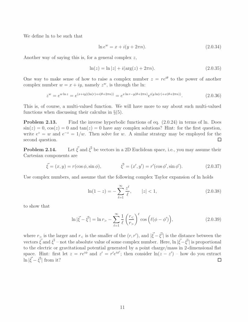
We define ln to be such that

ln ew = x+ i(y + 2πn). (2.0.34)

Another way of saying this is, for a general complex z,

ln(z) = ln |z|+ i(arg(z) + 2πn). (2.0.35)

One way to make sense of how to raise a complex number z = reiθ to the power of anothercomplex number w = x+ iy, namely zw, is through the ln:

zw = ew ln z = e(x+iy)(ln(r)+i(θ+2πn)) = ex ln r−y(θ+2πn)ei(y ln(r)+x(θ+2πn)). (2.0.36)

This is, of course, a multi-valued function. We will have more to say about such multi-valuedfunctions when discussing their calculus in §(5).

Problem 2.13. Find the inverse hyperbolic functions of eq. (2.0.24) in terms of ln. Doessin(z) = 0, cos(z) = 0 and tan(z) = 0 have any complex solutions? Hint: for the first question,write ez = w and e−z = 1/w. Then solve for w. A similar strategy may be employed for thesecond question.

Problem 2.14. Let ~ξ and ~ξ′ be vectors in a 2D Euclidean space, i.e., you may assume theirCartesian components are

~ξ = (x, y) = r(cosφ, sinφ), ~ξ′ = (x′, y′) = r′(cosφ′, sinφ′). (2.0.37)

Use complex numbers, and assume that the following complex Taylor expansion of ln holds

ln(1− z) = −∞∑

ℓ=1

zℓ

ℓ, |z| < 1, (2.0.38)

to show that

ln |~ξ − ~ξ′| = ln r> −∞∑

ℓ=1

1

ℓ

(r<r>

)ℓ

cos(ℓ(φ− φ′)

), (2.0.39)

where r> is the larger and r< is the smaller of the (r, r′), and |~ξ− ~ξ′| is the distance between the

vectors ~ξ and ~ξ′ – not the absolute value of some complex number. Here, ln |~ξ−~ξ′| is proportionalto the electric or gravitational potential generated by a point charge/mass in 2-dimensional flatspace. Hint: first let z = reiφ and z′ = r′eiφ

′; then consider ln(z − z′) – how do you extract

ln |~ξ − ~ξ′| from it?

11

3 Matrix Algebra: A Review

4In this section I will review some basic properties of matrices and matrix algebra, oftentimesusing index notation. We will assume all matrices have complex entries unless otherwise stated.This is intended to be warmup to the next section, where I will treat Linear Algebra from amore abstract point of view.

3.1 Basics, Matrix Operations, and Special types of matrices

Index notation, Einstein summation, Basic Matrix Operations Consider two ma-trices M and N . The ij component – the ith row and jth column of M and that of N can bewritten as

M ij and N i

j . (3.1.1)

As an example, if M is a 2× 2 matrix, we have

M =

[M1

1 M12

M21 M2

2

]. (3.1.2)

I prefer to write one index up and one down, because as we shall see in the abstract formulationof linear algebra below, the row and column indices may transform differently. However, it iscommon to see the notation Mij and M

ij , etc., too.A vector v can be written as

vi = (v1, v2, . . . , vD−1, vD). (3.1.3)

Here, v5 does not mean the fifth power of some quantity v, but rather the 5th component of thevector v.

The matrix multiplication M ·N can be written as

(M ·N)ij =D∑

k=1

M ikN

kj ≡M i

kNkj. (3.1.4)

In words: the ij component of the product MN , for a fixed i and fixed j, means we are takingthe ith row of M and “dotting” it into the jth column of N . In the second equality we haveemployed Einstein’s summation convention, which we will continue to do so in these notes:repeated indices are summed over their relevant range – in this case, k ∈ 1, 2, . . . , D. Forexample, if

M =

[a bc d

], N =

[1 23 4

], (3.1.5)

then

M ·N =

[a + 3b 2a+ 4bc+ 3d 2c+ 4d

]. (3.1.6)

4Much of the material here in this section were based on Chapter 1 of Cahill’s Physical Mathematics.

12

Note: M ikN

kj works for multiplication of non-square matrices M and N too, as long as the

number of columns ofM is equal to the number of rows of N , so that the sum involving k makessense.

Addition of M and N ; and multiplication of M by a complex number λ goes respectively as

(M +N)ij =M ij +N i

j (3.1.7)

and

(λM)ij = λM ij. (3.1.8)

Associativity The associativity of matrix multiplication means (AB)C = A(BC) = ABC.This can be seen using index notation

AikB

klC

lj = (AB)ilC

lj = Ai

k(BC)kj = (ABC)ij. (3.1.9)

Tr Tr(A) ≡ Aii denotes the trace of a square matrix A. The index notation makes it clear

the trace of AB is that of BA because

Tr [A · B] = AlkB

kl = Bk

lAlk = Tr [B · A] . (3.1.10)

This immediately implies the Tr is cyclic, in the sense that

Tr [X1 ·X2 · · ·XN ] = Tr [XN ·X1 ·X2 · · ·XN−1] = Tr [X2 ·X3 · · ·XN ·X1] . (3.1.11)

Problem 3.1. Prove the linearity of the Tr, namely for D × D matrices X and Y andcomplex number λ,

Tr [X + Y ] = Tr [X ] + Tr [Y ] , Tr [λX ] = λTr [X ] . (3.1.12)

Comment on whether it makes sense to define Tr(A) ≡ Aii, if A is not a square matrix.

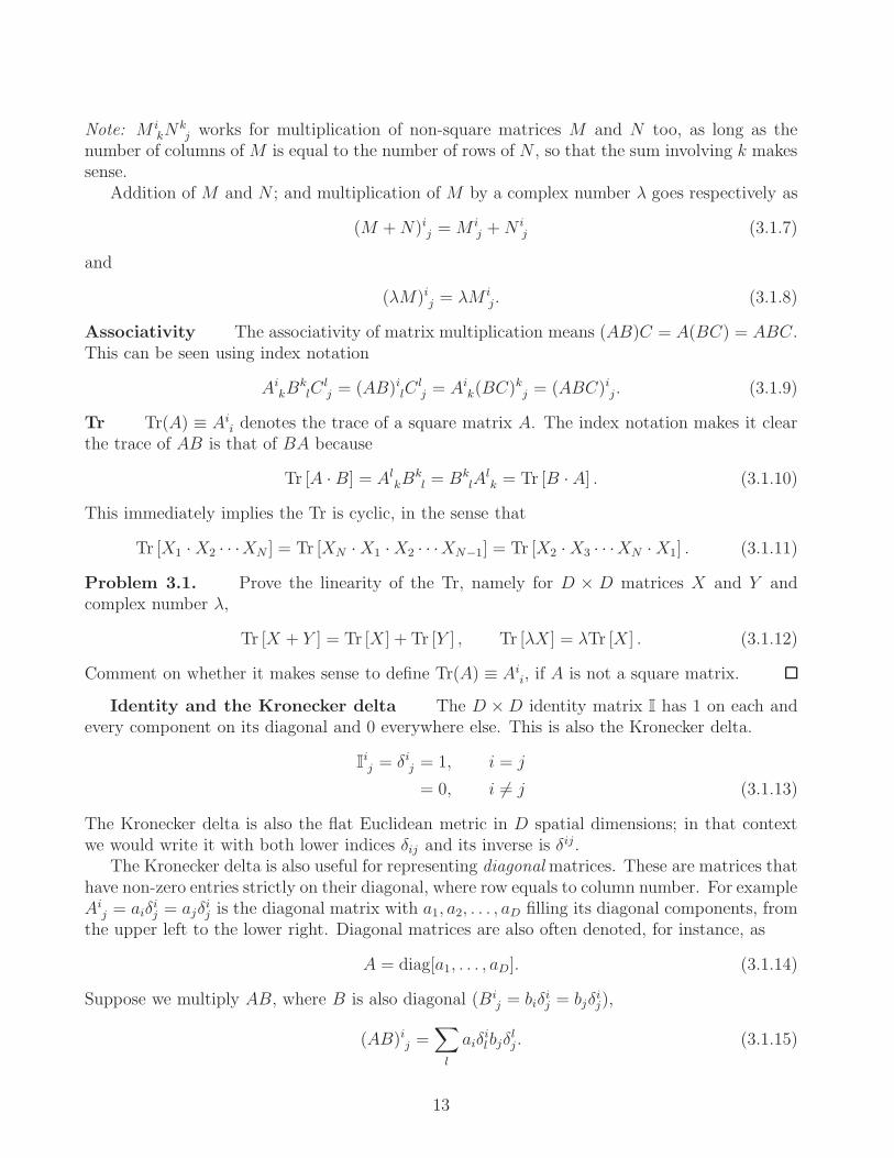
Identity and the Kronecker delta The D ×D identity matrix I has 1 on each andevery component on its diagonal and 0 everywhere else. This is also the Kronecker delta.

Iij = δij = 1, i = j

= 0, i 6= j (3.1.13)

The Kronecker delta is also the flat Euclidean metric in D spatial dimensions; in that contextwe would write it with both lower indices δij and its inverse is δij .

The Kronecker delta is also useful for representing diagonalmatrices. These are matrices thathave non-zero entries strictly on their diagonal, where row equals to column number. For exampleAi

j = aiδij = ajδ

ij is the diagonal matrix with a1, a2, . . . , aD filling its diagonal components, from

the upper left to the lower right. Diagonal matrices are also often denoted, for instance, as

A = diag[a1, . . . , aD]. (3.1.14)

Suppose we multiply AB, where B is also diagonal (Bij = biδ

ij = bjδ

ij),

(AB)ij =∑

l

aiδilbjδ

lj . (3.1.15)

13

If i 6= j there will be no l that is simultaneously equal to i and j; therefore either one or boththe Kronecker deltas are zero and the entire sum is zero. If i = j then when (and only when)l = i = j, the Kronecker deltas are both one, and

(AB)ij = aibj . (3.1.16)

This means we have shown, using index notation, that the product of diagonal matrices yieldsanother diagonal matrix.

(AB)ij = aibjδij (No sum over i, j). (3.1.17)

Transpose The transpose T of any matrix A is

(AT )ij = Aji. (3.1.18)

In words: the i row of AT is the ith column of A; the jth column of AT is the jth row of A. IfA is a (square) D ×D matrix, you reflect it along the diagonal to obtain AT .

Problem 3.2. Show using index notation that (A · B)T = BTAT .

Adjoint The adjoint † of any matrix is given by

(A†)ij = (Aji)∗ = (A∗)ji. (3.1.19)

In other words, A† = (AT )∗; to get A†, you start with A, take its transpose, then take its complexconjugate. An example is,

A =

[1 + i eiθ

x+ iy√10

], 0 ≤ θ < 2π, x, y ∈ R (3.1.20)

AT =

[1 + i x+ iy

eiθ√10

], A† =

[1− i x− iy

e−iθ√10

]. (3.1.21)

Orthogonal, Unitary, Symmetric, and Hermitian A D ×D matrix A is

1. Orthogonal if ATA = AAT = I. The set of real orthogonal matrices implement rotationsin a D-dimensional real (vector) space.

2. Unitary if A†A = AA† = I. Thus, a real unitary matrix is orthogonal. Moreover, unitarymatrices, like their real orthogonal counterparts, implement “rotations” in aD dimensionalcomplex (vector) space.

3. Symmetric if AT = A; anti-symmetric if AT = −A.

4. Hermitian if A† = A; anti-hermitian if A† = −A.Problem 3.3. Explain why, if A is an orthogonal matrix, it obeys the equation

AikA

jlδij = δkl. (3.1.22)

Now explain why, if A is a unitary matrix, it obeys the equation

(Aik)

∗Ajlδij = δkl. (3.1.23)

14

Problem 3.4. Prove that (AB)T = BTAT and (AB)† = B†A†. This means if A and B areorthogonal, then AB is orthogonal; and if A and B are unitary AB is unitary. Can you explainwhy?

Simple examples of a unitary, symmetric and Hermitian matrix are, respectively (from left toright):

[eiθ 00 eiδ

],

[eiθ XX eiδ

],

[ √109 1− i

1 + i θδ

], θ, δ ∈ R. (3.1.24)

3.2 Determinants, Linear (In)dependence, Inverses and Eigensys-

tems

Levi-Civita symbol and the Determinant We will now define the determinant of aD ×D matrix A through the Levi-Civita symbol ǫi1i2...iD−1iD :

detA ≡ ǫi1i2...iD−1iDAi11A

i22 . . . A

iD−1

D−1AiD

D. (3.2.1)

Every index on the Levi-Civita runs from 1 through D. This definition is equivalent to the usualco-factor expansion definition. The D-dimensional Levi-Civita symbol is defined through thefollowing properties.

• It is completely antisymmetric in its indices. This means swapping any of the indicesia ↔ ib (for a 6= b) will return

ǫi1i2...ia−1iaia+1...ib−1ibib+1...iD−1iD = −ǫi1i2...ia−1ibia+1...ib−1iaib+1...iD−1iD . (3.2.2)

• In matrix algebra and flat Euclidean space, ǫ123...D = ǫ123...D ≡ 1.5

These are sufficient to define every component of the Levi-Civita symbol. Because ǫ is fully anti-symmetric, if any of its D indices are the same, say ia = ib, then the Levi-Civita symbol returnszero. (Why?) Whenever i1 . . . iD are distinct indices, ǫi1i2...iD−1iD is really the sign of the per-mutation (≡ (−)nunber of swaps of index pairs) that brings 1, 2, . . . , D− 1, D to i1, i2, . . . , iD−1, iD.Hence, ǫi1i2...iD−1iD is +1 when it takes zero/even number of swaps, and −1 when it takes odd.

For example, in the 2 dimensional case ǫ11 = ǫ22 = 0; whereas it takes one swap to go from12 to 21. Therefore,

1 = ǫ12 = −ǫ21. (3.2.3)

In the 3 dimensional case,

1 = ǫ123 = −ǫ213 = −ǫ321 = −ǫ132 = ǫ231 = ǫ312. (3.2.4)

Properties of the determinant include

detAT = detA, det(A · B) = detA · detB, detA−1 =1

detA, (3.2.5)

5In Lorentzian flat spacetimes, the Levi-Civita tensor with upper indices will need to be carefully distinguishedfrom its counterpart with lower indices.

15

for square matrices A and B. As a simple example, let us use eq. (3.2.1) to calculate thedeterminant of

A =

[a bc d

]. (3.2.6)

Remember the only non-zero components of ǫi1i2 are ǫ12 = 1 and ǫ21 = −1.

detA = ǫ12A11A

22 + ǫ21A

21A

12 = A1

1A22 − A2

1A12

= ad− bc. (3.2.7)

Linear (in)dependence Given a set of D vectors v1, . . . , vD, we say one of them islinearly dependent (say vi) if we can express it in as a sum of multiples of the rest of the vectors,

vi =D−1∑

j 6=i

χjvj for some χj ∈ C. (3.2.8)

We say the D vectors are linearly independent if none of the vectors are linearly dependent onthe rest.

Det as test of linear independence If we view the columns or rows of a D × D matrixA as vectors and if these D vectors are linearly dependent, then the determinant of A is zero.This is because of the antisymmetric nature of the Levi-Civita symbol. Moreover, supposedetA 6= 0. Cramer’s rule (cf. eq. (3.2.12) below) tells us the inverse A−1 exists. In fact, forfinite dimensional matrix A, its inverse A−1 is unique. That means the only solution to theD-component row (or column) vector w, obeying w ·A = 0 (or, A · w = 0), is w = 0. And sincew · A (or A · w) describes the linear combination of the rows (or, columns) of A; this indicatesthey must be linearly independent whenever detA 6= 0.

For a square matrix A, detA = 0 iff (≡ if and only if) its columns and rowsare linearly dependent. Equivalently, detA 6= 0 iff its columns and rows are linearlyindependent.

Problem 3.5. If the columns of a square matrix A are linearly dependent, use eq. (3.2.1)to prove that detA = 0. Hint: use the antisymmetric nature of the Levi-Civita symbol.

Problem 3.6. Show that, for a D ×D matrix A and some complex number λ,

det(λA) = λD detA. (3.2.9)

Hint: this follows almost directly from eq. (3.2.1).

Problem 3.7. Relation to cofactor expansion The co-factor expansion definition of thedeterminant is

detA =D∑

i=1

AikC

ik, (3.2.10)

16

where k is an arbitrary integer from 1 through D. The C ik is (−)i+k times the determinant of

the (D − 1) × (D − 1) matrix formed from removing the ith row and kth column of A. (Thisdefinition sums over the row numbers; it is actually equally valid to define it as a sum overcolumn numbers.)

As a 3× 3 example, we have

det

a b cd e fg h l

= b(−)1+2 det

[d fg l

]+ e(−)2+2 det

[a cg l

]+ h(−)3+2 det

[a cd f

].

(3.2.11)

Cramer’s rule Can you show the equivalence of equations (3.2.1) and (3.2.10)? Can youalso show that

δkl detA =D∑

i=1

AikC

il? (3.2.12)

That is, show that when k 6= l, the sum on the right hand side is zero. What does eq. (3.2.12)tell us about (A−1)li?

Hint: start from the left-hand-side, namely

detA = ǫj1...jDAj11 . . . A

jDD (3.2.13)

= Aik

(ǫj1...jk−1ijk+1...jDA

j11 . . . A

jk−1

k−1Ajk+1

k+1 . . . AjD

D

),

where k is an arbitrary integer in the set 1, 2, 3, . . . , D − 1, D. Examine the term in theparenthesis. First shift the index i, which is located at the kth slot from the left, to the ithslot. Then argue why the result is (−)i+k times the determinant of A with the ith row and kthcolumn removed.

Pauli Matrices The 2 × 2 identity together with the Pauli matrices are Hermitianmatrices.

σ0 ≡[1 00 1

], σ1 ≡

[0 11 0

], σ2 ≡

[0 −ii 0

], σ3 ≡

[1 00 −1

](3.2.14)

Problem 3.8. Let pµ ≡ (p0, p1, p2, p3) be a 4-component collection of complex numbers.Verify the following determinant, relevant for the study of Lorentz symmetry in 4-dimensionalflat spacetime,

det pµσµ =

∑

0≤µ,ν≤3

ηµνpµpν ≡ p2, (3.2.15)

where pµσµ ≡

∑0≤µ≤3 pµσ

µ and

ηµν ≡

1 0 0 00 −1 0 00 0 −1 00 0 0 −1

. (3.2.16)

17

(This is the metric in 4 dimensional flat “Minkowski” spacetime.) Verify, for i, j, k ∈ 1, 2, 3,

det σ0 = 1, det σi = −1, Tr[σ0]= 2, Tr

[σi]= 0 (3.2.17)

σiσj = δijI+ i∑

1≤k≤3

ǫijkσk, σ2σiσ2 = −(σi)∗. (3.2.18)

Also use the antisymmetric nature of the Levi-Civita symbol to aruge that

θiθjǫijk = 0. (3.2.19)

Can you use these facts to calculate

U(~θ) ≡ exp

[− i

2

3∑

j=1

θjσj

]≡ e−(i/2)~θ·~σ? (3.2.20)

(Hint: Taylor expand expX =∑∞

ℓ=0Xℓ/ℓ!, followed by applying the first relation in eq. (3.2.18).)

For now, assume θi can be complex; later on you’d need to specialize to θi being real. Showthat any 2 × 2 complex matrix A can be built from pµσ

µ by choosing the pµs appropriately.Then compute (1/2)Tr [pµσ

µσν ], for ν = 0, 1, 2, 3, and comment on how the trace can be used,given A, to solve for the pµ in the equation

pµσµ = A. (3.2.21)

Inverse The inverse of the D ×D matrix A is defined to be

A−1A = AA−1 = I. (3.2.22)

The inverse A−1 of a finite dimensional matrix A is unique; moreover, the left A−1A = I andright inverses AA−1 = I are the same object. The inverse exists if and only if (≡ iff) detA 6= 0.

Problem 3.9. How does eq. (3.2.12) allow us to write down the inverse matrix (A−1)ik?

Problem 3.10. Why are the left and right inverses of (an invertible) matrix A the same?Hint: Consider LA = I and AR = I; for the first, multiply R on both sides from the right.

Problem 3.11. Prove that (A−1)T = (AT )−1 and (A−1)† = (A†)−1.

Eigenvectors and Eigenvalues If A is a D × D matrix, v is its (D-component)eigenvector with eigenvalue λ if it obeys

Aijv

j = λvi. (3.2.23)

This means

(Aij − λδij)v

j = 0 (3.2.24)

18

has non-trivial solutions iff

PD(λ) ≡ det (A− λI) = 0. (3.2.25)

Equation (3.2.25) is known as the characteristic equation. For a D × D matrix, it gives us aDth degree polynomial PD(λ) for λ, whose roots are the eigenvalues of the matrix λ – the setof all eigenvalues of a matrix is called its spectrum. For each solution for λ, we then proceed tosolve for the vi in eq. (3.2.24). That there is always at least one solution – there could be more– for vi is because, since its determinant is zero, the columns of A − λI are necessarily linearlydependent. As already discussed above, this amounts to the statement that there is some sum ofmultiples of these columns (≡ “linear combination”) that yields zero – in fact, the componentsof vi are precisely the coefficients in this sum. If wi are these columns of A− λI,

A− λI ≡ [w1w2 . . . wD] ⇒ (A− λI)v =∑

j

wjvj = 0. (3.2.26)

(Note that, if∑

j wjvj = 0 then

∑j wj(Kv

j) = 0 too, for any complex number K; in other words,eigenvectors are only defined up to an overall multiplicative constant.) Every D×D matrix hasD eigenvalues from solving the Dth order polynomial equation (3.2.25); from that, you can thenobtain D corresponding eigenvectors. Note, however, the eigenvalues can be repeated; when thisoccurs, it is known as a degenerate spectrum. Moreover, not all the eigenvectors are guaranteedto be linearly independent; i.e., some eigenvectors can turn out to be sums of multiples of othereigenvectors.

The Cayley-Hamilton theorem states that the matrix A satisfies its own characteristic equa-tion. In detail, if we express eq. (3.2.25) as

∑Di=0 qiλ

i = 0 (for appropriate complex constantsqi), then replace λi → Ai (namely, the ith power of λ with the ith power of A), we would find

PD(A) = 0. (3.2.27)

Any D ×D matrix A admits a Schur decomposition. Specifically, there is some unitary matrixU such that A can be brought to an upper triangular form, with its eigenvalues on the diagonal:

U †AU = diag(λ1, . . . , λD) +N, (3.2.28)

where N is strictly upper triangular, with N ij = 0 for j ≤ i. The Schur decomposition can be

proved via mathematical induction on the size of the matrix.A special case of the Schur decomposition occurs when all the off-diagonal elements are zero.

A D ×D matrix A can be diagonalized if there is some unitary matrix U such that

U †AU = diag(λ1, . . . , λD), (3.2.29)

where the λi are the eigenvalues of A. Each column of U is filled with a distinct unit lengtheigenvector of A. (Unit length means v†v = (vi)∗vjδij = 1.) In index notation,

AijU

jk = λkU

ik = U i

lδlkλk, (No sum over k). (3.2.30)

In matrix notation,

AU = Udiag[λ1, λ2, . . . , λD−1, λD]. (3.2.31)

19

Here, U jk for fixed k, is the kth eigenvector, and λk is the corresponding eigenvalue. By multi-

plying both sides with U †, we have

U †AU = D, Djl ≡ λlδ

jl (No sum over l). (3.2.32)

Some jargon: the null space of a matrix M is the space spanned by all vectors vi obeyingM · vi = 0. When we solve for the eigenvector of A by solving (A− λI) · v, we are really solvingfor the null space of the matrix M ≡ A − λI, because for a fixed eigenvalue λ, there could bemore than one solution – that’s what we mean by degeneracy.

Real symmetric matrices can be always diagonalized via an orthogonal transformation. Com-plex Hermitian matrices can always be diagonalized via a unitary one. These statements canbe proved readily using their Schur decomposition. For, let A be Hermitian and U be a unitarymatrix such that

UAU † = diag(λ1, . . . , λD) +N, (3.2.33)

where N is strictly upper triangular. Now, if A is Hermitian, so is UAU †, because (UAU †)† =(U †)†A†U † = UAU †. Therefore,

(UAU †)† = UAU † ⇒ diag(λ∗1, . . . , λ∗D) +N † = diag(λ1, . . . , λD) +N. (3.2.34)

Because the transpose of a strictly upper triangular matrix returns a strictly lower triangularmatrix, we have a strictly lower triangular matrix N † plus a diagonal matrix (built out of thecomplex conjugate of the eigenvalues of A) equal to a diagonal one (built out of the eigenvaluesof A) plus a strictly upper triangular N . That means N = 0 and λl = λ∗l . That is, any HermitianA is diagonalizable and all its eigenvalues are real.

Unitary matrices can also always be diagonalized. In fact, all its eigenvalues λi lie on theunit circle on the complex plane, i.e., |λi| = 1. Suppose now A is unitary and U is anotherunitary matrix such that the Schur decomposition of A reads

UAU † =M, (3.2.35)

where M is an upper triangular matrix with the eigenvalues of A on its diagonal. Now, if A isunitary, so is UAU †, because

(UAU †

)†(UAU †) = UA†U †UAU † = UA†AU † = UU † = I. (3.2.36)

That means

M †M = I ⇒ (M †M)kl = (M †)ksMsl =∑

s

MskM

sl = δijM i

kMjl = δkl, (3.2.37)

where we have recalled eq. (3.1.23) in the last equality. If wi denotes the ith column of M , theunitary nature of M implies all its columns are orthogonal to each other and each column haslength one. Since M is upper triangular, we see that the only non-zero component of the firstcolumn is its first row, i.e., wi

1 = M i1 = λ1δ

i1. Unit length means w†

1w1 = 1 ⇒ |λ1|2 = 1. Thatw1 is orthogonal to every other column wi>1 means the latter have their first rows equal to zero;M1

1M1l = λ1M

1l = 0 ⇒M1

l = 0 for l 6= 1 – remember M11 = λ1 itself cannot be zero because it

20

lies on the unit circle on the complex plane. Now, since its first component is necessarily zero,the only non-zero component of the second column is its second row, i.e., wi

2 =M i2 = λ2δ

i2. Unit

length again means |λ2|2 = 1. And, by demanding that w2 be orthogonal to every other column

means their second components are zero: M22M

2l = λ2M

2l = 0 ⇒ M2

l = 0 for l > 2 – where,

again,M22 = λ2 cannot be zero because it lies on the complex plane unit circle. By induction on

the column number, we see that the only non-zero component of the ith column is the ith row.That is, any unitary A is diagonalizable and all its eigenvalues lie on the circle: |λ1≤i≤D| = 1.

Diagonalization example As an example, let’s diagonalize σ2 from eq. (8.1.26).

P2(λ) = det

[−λ −ii −λ

]= λ2 − 1 = 0 (3.2.38)

(We can even check Caley-Hamilton here: P2(σ2) = (σ2)2 − I = I− I = 0; see eq. (3.2.18).) The

solutions are λ = ±1 and[∓1 −ii ∓1

] [v1

v2

]=

[00

]⇒ v1± = ∓iv2±. (3.2.39)

The subscripts on v refer to their eigenvalues, namely

σ2v± = ±v±. (3.2.40)

By choosing v2 = 1/√2, we can check (vi±)

∗vj±δij = 1 and therefore the normalized eigenvectorsare

v± =1√2

[∓i1

]. (3.2.41)

Furthermore you can check directly that eq. (3.2.40) is satisfied. We therefore have

(1√2

[i 1−i 1

])

︸ ︷︷ ︸≡U†

σ2

(1√2

[−i i1 1

])

︸ ︷︷ ︸≡U

=

[1 00 −1

]. (3.2.42)

An example of a matrix that cannot be diagonalized is

A ≡[0 01 0

]. (3.2.43)

The characteristic equation is λ2 = 0, so both eigenvalues are zero. Therefore A− λI = A, and[0 01 0

] [v1

v2

]=

[00

]⇒ v1 = 0, v2 arbitrary. (3.2.44)

There is a repeated eigenvalue of 0, but there is only one linearly independent eigenvector (0, 1).It is not possible to build a unitary 2 × 2 matrix U whose columns are distinct unit lengtheigenvectors of σ2.

Problem 3.12. Show how to go from eq. (3.2.30) to eq. (3.2.32) using index notation.

21

Problem 3.13. Use the Schur decomposition to explain why, for any matrix A, Tr [A] isequal to the sum of its eigenvalues and detA is equal to their product:

Tr [A] =D∑

l=1

λl, detA =D∏

l=1

λl. (3.2.45)

Hint: for detA, the key question is how to take the determinant of an upper triangular matrix.

Problem 3.14. For a strictly upper triangular matrix N , prove that N multiplied to itselfany number of times still returns a strictly upper triangular matrix. Can a strictly uppertriangular matrix be diagonalized? (Explain.)

Problem 3.15. Suppose A = UXU †, where U is a unitary matrix. If f(z) is a function of zthat can be Taylor expanded about some point z0, explain why f(A) = Uf(X)U †. Hint: Can youexplain why (UBU †)ℓ = UBℓU †, for B some arbitrary matrix, U unitary, and ℓ = 1, 2, 3, . . . ?

Problem 3.16. Can you provide a simple explanation to why the eigenvalues λl of aunitary matrix are always of unit absolute magnitude; i.e. why are the |λl| = 1?

Problem 3.17. Simplified example of neutrino oscillations. We begin with the observationthat the solution to the first order equation

i∂tψ(t) = Eψ(t), (3.2.46)

for E some real constant, is

ψ(t) = e−iEtψ0. (3.2.47)

The ψ0 is some arbitrary (possibly complex) constant, corresponding to the initial conditionψ(t = 0). Now solve the matrix differential equation

i∂tN(t) = HN(t), N(t) ≡[ν1(t)ν2(t)

], (3.2.48)

with the initial condition – describing the production of ν1-type of neutrino, say –

[ν1(t = 0)ν2(t = 0)

]=

[10

], (3.2.49)

where the Hamiltonian H is

H ≡[p 00 p

]+

1

4pM, (3.2.50)

M ≡[m2

1 +m22 + (m2

1 −m22) cos(2θ) (m2

1 −m22) sin(2θ)

(m21 −m2

2) sin(2θ) m21 +m2

2 + (m22 −m2

1) cos(2θ)

]. (3.2.51)

22

The p is the magnitude of the momentum, m1,2 are masses, and θ is the “mixing angle”. Thencalculate

P1→1 ≡∣∣∣∣N(t)†

[10

]∣∣∣∣2

and P1→2 ≡∣∣∣∣N(t)†

[01

]∣∣∣∣2

. (3.2.52)

Express P1→1 and P1→2 in terms of ∆m2 ≡ m21 −m2

2. (In quantum mechanics, they respectivelycorrespond to the probability of observing the neutrinos ν1 and ν2 at time t > 0, given ν1 wasproduced at t = 0.) Hint: Start by diagonalizing M = UTAU where

U ≡[

cos θ sin θ− sin θ cos θ

]. (3.2.53)

The UN(t) is known as the “mass-eigenstate” basis. Can you comment on why? Note that, inthe highly relativistic limit, the energy E of a particle of mass m is

E =√p2 +m2 → p+

m2

2p+O(1/p2). (3.2.54)

Note: In this problem, we have implicitly set ~ = c = 1, where ~ is the reduced Planck’s constantand c is the speed of light in vacuum.

3.3 Special Topic 1: 2D real orthogonal matrices

In this subsection we will illustrate what a real orthogonal matrix is by studying the 2D casein some detail. Let A be such a 2 × 2 real orthogonal matrix. We will begin by writing itscomponents as follows

A ≡[v1 v2

w1 w2

]. (3.3.1)

(As we will see, it is useful to think of v1,2 and w1,2 as components of 2D vectors.) That A isorthogonal means AAT = I.

[v1 v2

w1 w2

]·[v1 w1

v2 w2

]=

[~v · ~v ~v · ~w~w · ~v ~w · ~w

]=

[1 00 1

]. (3.3.2)

This translates to: ~w2 ≡ ~w · ~w = 1, ~v2 ≡ ~v · ~v = 1 (length of both the 2D vectors are one);and ~w · ~v = 0 (the two vectors are perpendicular). In 2D any vector can be expressed in polarcoordinates; for example, the Cartesian components of ~v are

vi = r(cosφ, sinφ), r ≥ 0, φ ∈ [0, 2π). (3.3.3)

But ~v2 = 1 means r = 1. Similarly,

wi = (cosφ′, sinφ′), φ′ ∈ [0, 2π). (3.3.4)

Because ~v and ~w are perpendicular,

~v · ~w = cosφ · cos φ′ + sinφ · sinφ′ = cos(φ− φ′) = 0. (3.3.5)

23

This means φ′ = φ± π/2. (Why?) Furthermore

wi = (cos(φ± π/2), sin(φ± π/2)) = (∓ sin(φ),± cos(φ)). (3.3.6)

What we have figured out is that, any real orthogonal matrix can be parametrized by an angle0 ≤ φ < 2π; and for each φ there are two distinct solutions.

R1(φ) =

[cosφ sin φ− sinφ cosφ

], R2(φ) =

[cosφ sin φsin φ − cosφ

]. (3.3.7)

By a direct calculation you can check that R1(φ > 0) rotates an arbitrary 2D vector clockwiseby φ. Whereas, R2(φ > 0) rotates the vector, followed by flipping the sign of its y-component;this is because

R2(φ) =

[1 00 −1

]· R1(φ). (3.3.8)

In other words, the R2(φ = 0) in eq. (3.3.7) corresponds to a “parity flip” where the vector isreflected about the x-axis.

Problem 3.18. What about the matrix that reflects 2D vectors about the y-axis? Whatvalue of θ in R2(θ) would it correspond to?

Find the determinants of R1(φ) and R2(φ). You should be able to use that to argue, thereis no θ0 such that R1(θ0) = R2(θ0). Also verify that

R1(φ)R1(φ′) = R1(φ+ φ′). (3.3.9)

This makes geometric sense: rotating a vector clockwise by φ then by φ′ should be the same asrotation by φ+φ′. Mathematically speaking, this composition law in eq. (3.3.9) tells us rotationsform the SO2 group. The set of D × D real orthogonal matrices obeying RTR = I, includingboth rotations and reflections, forms the group OD. The group involving only rotations is knownas SOD; where the ‘S’ stands for “special” (≡ determinant equals one).

Problem 3.19. 2× 2 Unitary Matrices. Can you construct the most general 2× 2 unitarymatrix? First argue that the most general complex 2D vector ~v that satisfies ~v†~v = 1 is

vi = eiφ1(cos θ, eiφ2 sin θ), φ1,2, θ ∈ [0, 2π). (3.3.10)

Then consider ~v† ~w = 0, where

wi = eiφ′1(cos θ′, eiφ

′2 sin θ′), φ′

1,2, θ′ ∈ [0, 2π). (3.3.11)

You should arrive at

sin(θ) sin(θ′)ei(φ′2−φ2) + cos(θ) cos(θ′) = 0. (3.3.12)

By taking the real and imaginary parts of this equation, argue that

φ′2 = φ2, θ = θ′ ± π

2. (3.3.13)

24

or

φ′2 = φ2 + π, θ = −θ′ ± π

2. (3.3.14)

From these, deduce that the most general 2 × 2 unitary matrix U can be built from the mostgeneral real orthogonal one O(θ) via

U =

[eiφ1 00 eiφ2

]·O(θ) ·

[1 00 eiφ3

]. (3.3.15)

As a simple check: note that ~v†~v = ~w† ~w = 1 together with ~v† ~w = 0 provides 4 constraintsfor 8 parameters – 4 complex entries of a 2 × 2 matrix – and therefore we should have 4 freeparameters left.

Bonus problem: By imposing detU = 1, can you connect eq. (3.3.15) to eq. (3.2.20)?

25

4 Linear Algebra

4.1 Definition

Loosely speaking, the notion of a vector space – as the name suggests – amounts to abstractingthe algebraic properties – addition of vectors, multiplication of a vector by a number, etc. –obeyed by the familiar D ∈ 1, 2, 3, . . . dimensional Euclidean space RD. We will discuss thelinear algebra of vector spaces using Paul Dirac’s bra-ket notation. This will not only help youunderstand the logical foundations of linear algebra and the matrix algebra you encounteredearlier, it will also prepare you for the study of quantum theory, which is built entirely on thetheory of both finite and infinite dimensional vector spaces.6

We will consider a vector space over complex numbers. A member of the vector space willbe denoted as |α〉; we will use the words “ket”, “vector” and “state” interchangeably in whatfollows. We will allude to aspects of quantum theory, but point out everything we state hereholds in a more general context; i.e., quantum theory is not necessary but merely an application– albeit a very important one for physics. For now α is just some arbitrary label, but lateron it will often correspond to the eigenvalue of some linear operator. We may also use α asan enumeration label, where |α〉 is the αth element in the collection of vectors. In quantummechanics, a physical system is postulated to be completely described by some |α〉 in a vectorspace, whose time evolution is governed by some Hamiltonian. (The latter is what Schrodinger’sequation is about.)

Here is what defines a “vector space over complex numbers”:

1. Addition Any two vectors can be added to yield another vector

|α〉+ |β〉 = |γ〉 . (4.1.1)

Addition is commutative and associative:

|α〉+ |β〉 = |β〉+ |α〉 (4.1.2)

|α〉+ (|β〉+ |γ〉) = (|α〉+ |β〉) + |γ〉 . (4.1.3)

2. Additive identity (zero vector) and existence of inverse There is a zero vector|zero〉 – which can be gotten by multiplying any vector by 0, i.e.,

0 |α〉 = |zero〉 (4.1.4)

– that acts as an additive identity.7 Namely, adding |zero〉 to any vector returns the vectoritself:

|zero〉+ |β〉 = |β〉 . (4.1.5)

For any vector |α〉 there exists an additive inverse; if + is the usual addition, then theinverse of |α〉 is just (−1) |α〉.

|α〉+ (− |α〉) = |zero〉 . (4.1.6)6The material in this section of our notes was drawn heavily from the contents and problems provided in

Chapter 1 of Sakurai’s Modern Quantum Mechanics.7In this section we will be careful and denote the zero vector as |zero〉. For the rest of the notes, whenever

the context is clear, we will often use 0 to denote the zero vector.

26

3. Multiplication by scalar Any ket can be multiplied by an arbitrary complex numberc to yield another vector

c |α〉 = |γ〉 . (4.1.7)

(In quantum theory, |α〉 and c |α〉 are postulated to describe the same system.) Thismultiplication is distributive with respect to both vector and scalar addition; if a and bare arbitrary complex numbers,

a(|α〉+ |β〉) = a |α〉+ a |β〉 (4.1.8)

(a+ b) |α〉 = a |α〉+ b |α〉 . (4.1.9)

Note: If you define a “vector space over scalars,” where the scalars can be more general objectsthan complex numbers, then in addition to the above axioms, we have to add: (I) Associativity ofscalar multiplication, where a(b |α〉) = (ab) |α〉 for any scalars a, b and vector |α〉; (II) Existenceof a scalar identity 1, where 1 |α〉 = |α〉.

Examples The Euclidean space RD itself, the space of D-tuples of real numbers

|~a〉 ≡ (a1, a2, . . . , aD), (4.1.10)

with + being the usual addition operation is, of course, the example of a vector space. We shallcheck explicitly that RD does in fact satisfy all the above axioms. To begin, let

|~v〉 = (v1, v2, . . . , vD),

|~w〉 = (w1, w2, . . . , wD) and (4.1.11)

|~x〉 = (x1, x2, . . . , xD) (4.1.12)

be vectors in RD.

1. Addition Any two vectors can be added to yield another vector

|~v〉+ |~w〉 = (v1 + w1, . . . , vD + wD) ≡ |~v + ~w〉 . (4.1.13)

Addition is commutative and associative because we are adding/subtracting the vectorscomponent-by-component:

|~v〉+ |~w〉 = |~v + ~w〉 = (v1 + w1, . . . , vD + wD)

= (w1 + v1, . . . , wD + vD)

= |~w〉+ |~v〉 = |~w + ~v〉 , (4.1.14)

|~v〉+ |~w〉+ |~x〉 = (v1 + w1 + x1, . . . , vD + wD + xD)

= (v1 + (w1 + x1), . . . , vD + (wD + xD))

= ((v1 + w1) + x1, . . . , (vD + wD) + xD)

= |~v〉+ (|~w〉+ |~x〉) = (|~v〉+ |~w〉) + |~x〉 = |~v + ~w + ~x〉 . (4.1.15)

27

2. Additive identity (zero vector) and existence of inverse There is a zero vector|zero〉 – which can be gotten by multiplying any vector by 0, i.e.,

0 |~v〉 = 0(v1, . . . , vD) = (0, . . . , 0) = |zero〉 (4.1.16)

– that acts as an additive identity. Namely, adding |zero〉 to any vector returns the vectoritself:

|zero〉+ |~w〉 = (0, . . . , 0) + (w1, . . . , wD) = |~w〉 . (4.1.17)

For any vector |~x〉 there exists an additive inverse; in fact, the inverse of |~x〉 is just(−1) |~x〉 = |−~x〉.

|~x〉+ (− |~x〉) = (x1, . . . , xD)− (x1, . . . , xD) = |zero〉 . (4.1.18)

3. Multiplication by scalar Any ket can be multiplied by an arbitrary real number cto yield another vector

c |~v〉 = c(v1, . . . , vD) = (cv1, . . . , cvD) ≡ |c~v〉 . (4.1.19)

This multiplication is distributive with respect to both vector and scalar addition; if a andb are arbitrary real numbers,

a(|~v〉+ |~w〉) = (av1 + aw1, av2 + aw2, . . . , avD + awD)

= |a~v〉+ |a~w〉 = a |~v〉+ a |~w〉 , (4.1.20)

(a+ b) |~x〉 = (ax1 + bx1, . . . , axD + bxD)

= |a~x〉+ |b~x〉 = a |~x〉+ b |~x〉 . (4.1.21)

The following are some further examples of vector spaces.

1. The space of polynomials with complex coefficients.

2. The space of square integrable functions on RD (where D is an arbitrary integer greateror equal to 1); i.e., all functions f(~x) such that

∫RD dD~x|f(~x)|2 <∞.

3. The space of all homogeneous solutions to a linear (ordinary or partial) differential equa-tion.

4. The space of M ×N matrices of complex numbers, where M and N are arbitrary integersgreater or equal to 1.

Problem 4.1. Prove that the examples in (1), (3), and (4) are indeed vector spaces, byrunning through the above axioms.

28

Linear (in)dependence, Basis, Dimension Suppose we pick N vectors from a vectorspace, and find that one of them can be expressed as a linear combination of the rest,

|N〉 =N−1∑

i=1

ci |i〉 , (4.1.22)

where the ci are complex numbers. Then we say that this set of N vectors are linearlydependent. Suppose we have pickedM vectors |1〉 , |2〉 , |3〉 , . . . , |M〉 such that they are linearlyindependent, i.e., no vector is a linear combination of any others, and suppose further that anyarbitrary vector |α〉 from the vector space can now be expressed as a linear combination (akasuperposition) of these vectors

|α〉 =D∑

i=1

χi |i〉 , χi ∈ C. (4.1.23)

In other words, we now have a maximal number of linearly independent vectors – then, M iscalled the dimension of the vector space. The |i〉 |i = 1, 2, . . . ,M is a complete set of basisvectors; and such a set of (basis) vectors is said to span the vector space.

For instance, for the D-tuple |~a〉 ≡ (a1, . . . , aD) from the real vector space of RD, we maychoose

|1〉 = (1, 0, 0, . . . ), |2〉 = (0, 1, 0, 0, . . . ),

|3〉 = (0, 0, 1, 0, 0, . . . ), . . . |D〉 = (0, 0, . . . , 0, 0, 1). (4.1.24)

Then, any arbitrary |~a〉 can be written as

|~a〉 = (a1, . . . , aD) =

D∑

i=1

ai |i〉 . (4.1.25)

The basis vectors are the |i〉 and the dimension is D.

Problem 4.2. Is the space of polynomials of complex coefficients of degree less than orequal to (n ≥ 1) a vector space? (Namely, this is the set of polynomials of the form Pn(x) =c0 + c1x+ · · ·+ cnx

n, where the ci|i = 1, 2, . . . , n are complex numbers.) If so, write down aset of basis vectors. What is its dimension? Answer the same questions for the space of D ×Dmatrices of complex numbers.

4.2 Inner Products

In Euclidean D-space RD the ordinary dot product, between the real vectors |~a〉 ≡ (a1, . . . , aD)

and |~b〉 ≡ (b1, . . . , bD), is defined as

~a ·~b ≡D∑

i=1

aibi = δijaibj . (4.2.1)

29

The inner product of linear algebra is again an abstraction of this notion of the dot product,where the analog of ~a · ~b will be denoted as 〈~a|~b〉. Like the dot product for Euclidean space,the inner product will allow us to define a notion of the length of vectors and angles betweendifferent vectors.

Dual/“bra” space Given a vector space, an inner product is defined by first introducinga dual space (aka bra space) to this vector space. Specifically, given a vector |α〉 we write itsdual as 〈α|. We also introduce the notation

|α〉† ≡ 〈α| . (4.2.2)

Importantly, for some complex number c, the dual of c |α〉 is(c |α〉)† ≡ c∗ 〈α| . (4.2.3)

Moreover, for complex numbers a and b,

(a |α〉+ b |β〉)† ≡ a∗ 〈α|+ b∗ 〈β| . (4.2.4)

Since there is a one-to-one correspondence between the vector space and its dual, it is not difficultto see this dual space is indeed a vector space.

Now, the primary purpose of these dual vectors is that they act on vectors of the originalvector space to return a complex number:

〈α|β〉 ∈ C. (4.2.5)

Definition. The inner product is now defined by the following properties. For an arbitrarycomplex number c,

〈α| (|β〉+ |γ〉) = 〈α|β〉+ 〈α| γ〉 (4.2.6)

〈α| (c |β〉) = c 〈α|β〉 (4.2.7)

〈α|β〉∗ = 〈α|β〉 = 〈β|α〉 (4.2.8)

〈α|α〉 ≥ 0 (4.2.9)

and

〈α|α〉 = 0 (4.2.10)

if and only if |α〉 is the zero vector.Some words on notation here. Especially in the math literature, the bra-ket notation is not

used. There, the inner product is often denoted by (α, β), where α and β are vectors. Then thedefining properties of the inner product would read instead

(α, β + γ) = (α, β) + (α, γ) (4.2.11)

(α, β)∗ = (α, β) = (β, α) (4.2.12)

(α, α) ≥ 0 (4.2.13)

and

(α, α) = 0 (4.2.14)

if and only if α is the zero vector.

30

Problem 4.3. Prove that 〈α|α〉 is a real number.

The following are examples of inner products.

• Take the D-tuple of complex numbers |α〉 ≡ (α1, . . . , αD) and |β〉 ≡ (β1, . . . , βD); anddefine the inner product to be

〈α|β〉 ≡D∑

i=1

(αi)∗βi = δij(αi)∗βj = α†β. (4.2.15)

• Consider the space of D×D complex matrices. Consider two such matrices X and Y anddefine their inner product to be

〈X|Y 〉 ≡ Tr[X†Y

]. (4.2.16)

Here, Tr means the matrix trace and X† is the adjoint of the matrix X .

• Consider the space of polynomials. Suppose |f〉 and |g〉 are two such polynomials of thevector space. Then

〈f | g〉 ≡∫ 1

−1

dxf(x)∗g(x) (4.2.17)

defines an inner product. Here, f(x) and g(x) indicates the polynomials are expressed interms of the variable x.

Problem 4.4. Prove the above examples are indeed inner products.

Problem 4.5. Prove the Schwarz inequality:

〈α|α〉 〈β|β〉 ≥ |〈α|β〉|2 . (4.2.18)

The analogy in Euclidean space is |~x|2|~y|2 ≥ |~x · ~y|2. Hint: Start with

(〈α|+ c∗ 〈β|) (|α〉+ c |β〉) ≥ 0. (4.2.19)

for any complex number c. (Why is this true?) Now choose an appropriate c to prove theSchwarz inequality.

Orthogonality Just as we would say two real vectors in RD are perpendicular (aka orthog-onal) when their dot product is zero, we may now define two vectors |α〉 and |β〉 in a vectorspace to be orthogonal when their inner product is zero:

〈α|β〉 = 0 = 〈β|α〉 . (4.2.20)

We also call√

〈α|α〉 the norm of the vector |α〉; recall, in Euclidean space, the analogous

|~x| =√~x · ~x. Given any vector |α〉 that is not the zero vector, we can always construct a vector

from it that is of unit length,

|α〉 ≡ |α〉√〈α|α〉

⇒ 〈α| α〉 = 1. (4.2.21)

31

Suppose we are given a set of basis vectors |i′〉 of a vector space. Through what is known asthe Gram-Schmidt process, one can always build from them a set of orthonormal basis vectors|i〉; where every basis vector has unit norm and is orthogonal to every other basis vector,

〈i| j〉 = δij . (4.2.22)

As you will see, just as vector calculus problems are often easier to analyze when you choose anorthogonal coordinate system, linear algebra problems are often easier to study when you usean orthonormal basis to describe your vector space.

Problem 4.6. Suppose |α〉 and |β〉 are linearly dependent – they are scalar multiples ofeach other. However, their inner product is zero. What are |α〉 and |β〉?

Problem 4.7. Let |1〉 , |2〉 , . . . , |N〉 be a set of N orthonormal vectors. Let |α〉 be anarbitrary vector lying in the same vector space. Show that the following vector constructed from|α〉 is orthogonal to all the |i〉.

|α〉 ≡ |α〉 −N∑

j=1

|j〉 〈j|α〉 . (4.2.23)

This result is key to the following Gram-Schmidt process.

Gram-Schmidt Let |α1〉 , |α2〉 , . . . , |αD〉 be a set of D linearly independent vectors thatspans some vector space. The Gram-Schmidt process is an iterative algorithm, based on theobservation in eq. (4.2.23), to generate from it a set of orthonormal set of basis vectors.

1. Take the first vector |α1〉 and normalize it to unit length:

|α1〉 =|α1〉√〈α1|α1〉

. (4.2.24)

2. Take the second vector |α2〉 and project out |α1〉:

|α′2〉 ≡ |α2〉 − |α1〉 〈α1|α2〉 , (4.2.25)

and normalize it to unit length

|α2〉 ≡|α′

2〉√〈α′

2|α′2〉. (4.2.26)

3. Take the third vector |α3〉 and project out |α1〉 and |α2〉:

|α′3〉 ≡ |α3〉 − |α1〉 〈α1|α3〉 − |α2〉 〈α2|α3〉 , (4.2.27)

then normalize it to unit length

|α3〉 ≡|α′

3〉√〈α′

3|α′3〉. (4.2.28)

32

4. Repeat . . . Take the ith vector |αi〉 and project out |α1〉 through |αi−1〉:

|α′i〉 ≡ |αi〉 −

i−1∑

j=1

|αj〉 〈αj|αi〉 , (4.2.29)

then normalize it to unit length

|αi〉 ≡|α′

i〉√〈α′

i|α′i〉. (4.2.30)

By construction, |αi〉 will be orthogonal to |α1〉 through |αi−1〉. Therefore, at the end of theprocess, we will have D mutually orthogonal and unit norm vectors. Because they are orthogonalthey are linearly independent – hence, we have succeeded in constructing an orthonormal set ofbasis vectors.

Example Here is a simple example in 3D Euclidean space endowed with the usual dotproduct. Let us have

|α1〉 =(2, 0, 0), |α2〉 =(1, 1, 1), |α3〉 =(1, 0, 1). (4.2.31)

You can check that these vectors are linearly independent by taking the determinant of the 3×3matrix formed from them. Alternatively, the fact that they generate a set of basis vectors fromthe Gram-Schmidt process also implies they are linearly independent.

Normalizing |α1〉 to unity,

|α1〉 =|α1〉√〈α1|α1〉

=(2, 0, 0)

2= (1, 0, 0). (4.2.32)

Next we project out |α1〉 from |α2〉.

|α′2〉 = |α2〉 − |α1〉 〈α1|α2〉 = (1, 1, 1)− (1, 0, 0)(1 + 0 + 0) = (0, 1, 1). (4.2.33)

Then we normalize it to unit length.

|α2〉 =|α′

2〉√〈α′

2|α′2〉

=(0, 1, 1)√

2. (4.2.34)

Next we project out |α1〉 and |α2〉 from |α3〉.

|α′3〉 = |α3〉 − |α1〉 〈α1|α3〉 − |α2〉 〈α2|α3〉

= (1, 0, 1)− (1, 0, 0)(1 + 0 + 0)− (0, 1, 1)√2

0 + 0 + 1√2

= (1, 0, 1)− (1, 0, 0)− (0, 1, 1)

2=

(0,−1

2,1

2

). (4.2.35)

Then we normalize it to unit length.

|α3〉 =|α′

3〉√〈α′

3|α′3〉

=(0,−1, 1)√

2. (4.2.36)

33

You can check that

|α1〉 = (1, 0, 0), |α2〉 =(0, 1, 1)√

2, |α3〉 =

(0,−1, 1)√2

, (4.2.37)

are mutually perpendicular and of unit length.

Problem 4.8. Consider the space of polynomials with complex coefficients. Let the innerproduct be

〈f | g〉 ≡∫ +1

−1

dxf(x)∗g(x). (4.2.38)

Starting from the set |0〉 = 1, |1〉 = x, |2〉 = x2, construct from them a set of orthonormalbasis vectors spanning the subspace of polynomials of degree equal to or less than 2. Compareyour results with the Legendre polynomials

Pℓ(x) ≡1

2ℓℓ!

dℓ

dxℓ(x2 − 1

)ℓ, ℓ = 0, 1, 2. (4.2.39)

Orthogonality and Linear independence. We close this subsection with an ob-servation. If a set of non-zero kets |i〉 |i = 1, 2, . . . , N − 1, N are orthogonal, then they arenecessarily linearly independent. This can be proved readily by contradiction. Suppose thesekets were linearly dependent. Then it must be possible to find non-zero complex numbers C isuch that

N∑

i=1

C i |i〉 = 0. (4.2.40)

If we now act 〈j| on this equation, for any j ∈ 1, 2, 3, . . . , N,N∑

i=1

C i 〈j| i〉 =N∑

i=1

C iδij 〈j| j〉 = Cj 〈j| j〉 = 0. (4.2.41)

That means all the Cj|j = 1, 2, . . . , N are in fact zero.A simple application of this observation is, if you have found D mutually orthogonal kets

|i〉 in a D dimensional vector space, then these kets form a basis. By normalizing them tounit length, you’d have obtained an orthonormal basis. Such an example is that of the Paulimatrices σµ|µ = 0, 1, 2, 3 in eq. (8.1.26). The vector space of 2 × 2 complex matrices is 4-dimensional, since there are 4 independent components. Moreover, we have already seen thatthe trace Tr

[X†Y

]is one way to define an inner product of matrices X and Y . Since

1

2Tr[(σµ)† σν

]=

1

2Tr [σµσν ] = δµν , µ, ν ∈ 0, 1, 2, 3, (4.2.42)

that means, by the argument just given, the 4 Pauli matrices σµ form an orthogonal set ofbasis vectors for the vector space of complex 2× 2 matrices. That means it must be possible tochoose pµ such that the superposition pµσ

µ is equal to any given 2× 2 complex matrix A. Infact,

pµσµ = A, ⇔ pµ =

1

2Tr [σµA] . (4.2.43)

34

4.3 Linear Operators

4.3.1 Definitions and Fundamental Concepts

In quantum theory, a physical observable is associated with a (Hermitian) linear operator actingon the vector space. What defines a linear operator? Let A be one. Firstly, when it acts fromthe left on a vector, it returns another vector

A |α〉 = |α′〉 . (4.3.1)

In other words, if you can tell me what you want the “output” |α′〉 to be, after A acts on anyvector of the vector space |α〉 – you’d have defined A itself. But that’s not all – linearity alsomeans, for otherwise arbitrary operators A and B and complex numbers c and d,

(A+B) |α〉 = A |α〉+B |α〉 (4.3.2)

A(c |α〉+ d |β〉) = c A |α〉+ d A |β〉 .

An operator always acts on a bra from the right, and returns another bra,

〈α|A = 〈α′| . (4.3.3)

Adjoint We denote the adjoint of the linear operator X , by taking the † of the ket X |α〉in the following way:

(X |α〉)† = 〈α|X†. (4.3.4)

Multiplication If X and Y are both linear operators, since Y |α〉 is a vector, we canapply X to it to obtain another vector, X(Y |α〉). This means we ought to be able to multiplyoperators, for e.g., XY . We will assume this multiplication is associative, namely

XY Z = (XY )Z = X(Y Z). (4.3.5)

Problem 4.9. By considering the adjoint of XY |α〉, where X and Y are arbitrary linearoperators and |α〉 is an arbitrary vector, prove that

(XY )† = Y †X†. (4.3.6)

Hint: take the adjoint of (XY ) |α〉 and X(Y |α〉).

Eigenvectors and eigenvalues An eigenvector of some linear operator A is a vectorthat, when acted upon by A, returns the vector itself multiplied by a complex number a:

X |a〉 = a |a〉 . (4.3.7)

This number a is called the eigenvalue of A.Ket-bra operator Notice that the product |α〉 〈β| can be considered a linear operator.

To see this, we apply it on some arbitrary vector |γ〉 and observe it returns the vector |α〉multiplied by a complex number describing the projection of |γ〉 on |β〉,

(|α〉 〈β|) |γ〉 = |α〉 (〈β| γ〉) = (〈β| γ〉) · |α〉 , (4.3.8)

35

as long as we assume these products are associative. It obeys the following “linearity” rules. If|α〉 〈β| and |α′〉 〈β ′| are two different ket-bra operators,

(|α〉 〈β|+ |α′〉 〈β ′|) |γ〉 = |α〉 〈β| γ〉+ |α′〉 〈β ′| γ〉 ; (4.3.9)

and for complex numbers c and d,

|α〉 〈β| (c |γ〉+ d |γ′〉) = c |α〉 〈β| γ〉+ d |α〉 〈β| γ′〉 . (4.3.10)

Problem 4.10. Show that

(|α〉 〈β|)† = |β〉 〈α| . (4.3.11)

Hint: Act |α〉 〈β| on an arbitrary vector, and then take its adjoint.

Projection operator The special case |α〉 〈α| acting on any vector |γ〉 will return|α〉 〈α| γ〉. Thus, we can view it as a projection operator – it takes an arbitrary vector andextracts the portion of it “parallel” to |α〉.

Identity The identity operator obeys

I |γ〉 = |γ〉 . (4.3.12)

Inverse The inverse of the operator X is still defined as one that obeys

X−1X = XX−1 = I. (4.3.13)

Strictly speaking, we need to distinguish between the left and right inverse, but in finite dimen-sional vector spaces, they are the same object.

Superposition, the identity operator, and vector components We will now seethat (square) matrices can be viewed as representations of linear operators on a vector space.Let |i〉 denote the basis orthonormal vectors of the vector space,

〈i| j〉 = δij . (4.3.14)

Then we may consider acting an linear operator X on some arbitrary vector |γ〉, which we willexpress as a linear combination of the |i〉:

|γ〉 =∑

i

γi |i〉 , γi ∈ C. (4.3.15)

By acting both sides with respect to 〈j|, we have

〈j| γ〉 = γj . (4.3.16)

In other words,

|γ〉 =∑

i

|i〉 〈i| γ〉 . (4.3.17)

36

Since |γ〉 was arbitrary, we have identified the identity operator as

I =∑

i

|i〉 〈i| . (4.3.18)

This is also often known as a completeness relation: summing over the ket-bra operators builtout of the orthonormal basis vectors of a vector space returns the unit (aka identity) operator.I acting on any vector yields the same vector.

Once a set of orthonormal basis vectors are chosen, notice from the expansion in eq. (4.3.17),that to specify a vector |γ〉 all we need to do is to specify the complex numbers 〈i| γ〉. Thesecan be arranged as a column vector; if the dimension of the vector space is D, then

|γ〉 =

〈1| γ〉〈2| γ〉〈3| γ〉. . .

〈D| γ〉

. (4.3.19)

The = is not quite an equality; rather it means “represented by,” in that this column vectorcontains as much information as eq. (4.3.17), provided the orthonormal basis vectors are known.

We may also express an arbitrary bra through a superposition of the basis bras 〈i|, usingeq. (4.3.18).

〈α| =∑

i

〈α| i〉 〈i| . (4.3.20)

Matrix elements Consider now some operator X acting on an arbitrary vector |γ〉, ex-pressed through the orthonormal basis vectors |i〉.

X |γ〉 =∑

i

X |i〉 〈i| γ〉 . (4.3.21)

We can insert an identity operator from the left,

X |γ〉 =∑

i,j

|j〉 〈j |X| i〉 〈i| γ〉 . (4.3.22)

We can also apply the lth basis bra 〈l| from the left on both sides and obtain

〈l|X |γ〉 =∑

i

〈l |X| i〉 〈i| γ〉 . (4.3.23)

Just as we read off the components of the vector in eq. (4.3.17) as a column vector, we can dothe same here. Again supposing a D dimensional vector space (for notational convenience),

X |γ〉 =

〈1 |X| 1〉 〈1 |X| 2〉 . . . 〈1 |X|D〉〈2 |X| 1〉 〈2 |X| 2〉 . . . 〈2 |X|D〉. . . . . . . . . . . .

〈D |X| 1〉 〈D |X| 2〉 . . . 〈D |X|D〉

〈1| γ〉〈2| γ〉〈3| γ〉. . .

〈D| γ〉

. (4.3.24)

37

In words: X acting on some vector |γ〉 can be represented by the column vector gotten fromacting the matrix 〈j |X| i〉, with row number j and column number i, acting on the columnvector 〈i| γ〉. In index notation, with8

X ij ≡ 〈i |X| j〉 and γj ≡ 〈j| γ〉 , (4.3.25)

we have

〈i|X |γ〉 = X ijγ

j . (4.3.26)

Since |γ〉 in eq. (4.3.22) was arbitrary, we may record that any linear operator X admits anket-bra operator expansion:

X =∑

i,j

|j〉 〈j |X| i〉 〈i| =∑

i,j

|j〉 Xji 〈i| . (4.3.27)

Equivalently, this result follows from inserting the completeness relation in eq. (4.3.18) on the

left and right ofX . We see that specifying the matrix Xji amounts to defining the linear operator

X itself.Vector Space of Linear Operators You may step through the axioms of Linear Algebra to

verify that the space of Linear operators is, in fact, a vector space itself. Given an orthonormalbasis |i〉 for the original vector space upon which these linear operators are acting, we see thatthe expansion in eq. (4.3.27) – which holds for an arbitrary linear operator X – teaches us theset of ket-bra operators

|j〉 〈i| |j, i = 1, 2, 3, . . . , D (4.3.28)

form the basis of the space of linear operators. The matrix elements 〈j |X| i〉 = Xji are the

expansion coefficients.Example What is the matrix representation of |β〉 〈α|? We apply 〈i| from the left and

|j〉 from the right to obtain the ij component

〈i| (|α〉 〈β|) |j〉 = 〈i|α〉 〈β| j〉 =αiβj. (4.3.29)

Products of operators We can consider Y X , where X and Y are linear operators. Byinserting the completeness relation in eq. (4.3.18),

Y X |γ〉 =∑

i,j,k

|k〉 〈k| Y |j〉 〈j |X| i〉 〈i| γ〉

=∑

k

|k〉 Y kjX

jiγ

i. (4.3.30)

The product Y X can therefore be represented as

Y X=

〈1 |Y | 1〉 〈1 |Y | 2〉 . . . 〈1 |Y |D〉〈2 |Y | 1〉 〈2 |Y | 2〉 . . . 〈2 |Y |D〉. . . . . . . . . . . .

〈D |Y | 1〉 〈D |Y | 2〉 . . . 〈D |Y |D〉

〈1 |X| 1〉 〈1 |X| 2〉 . . . 〈1 |X|D〉〈2 |X| 1〉 〈2 |X| 2〉 . . . 〈2 |X|D〉. . . . . . . . . . . .

〈D |X| 1〉 〈D |X| 2〉 . . . 〈D |X|D〉

.

(4.3.31)

8In this chapter on the abstract formulation of Linear Algebra, I use a · to denote a matrix (representation),in order to distinguish it from the linear operator itself.

38

Notice how the rules of matrix multiplication emerges from this abstract formulation of linearoperators acting on a vector space.

Inner product of two kets In an orthonormal basis, the inner product of |α〉 and |β〉 canbe written as a complex “dot product” because we may insert the completeness relation in eq.(4.3.18),

〈α|β〉 = 〈α |I|β〉 =∑

i

〈α| i〉 〈i|β〉 =δijαiβj = α†β. (4.3.32)

This means if 〈i| β〉 is the column vector representing |β〉 in a given orthonormal basis; then〈α| i〉, the adjoint of the column 〈i|α〉 representing |α〉, should be viewed as a row vector.

Furthermore, if |γ〉 has unit norm, then

1 = 〈γ| γ〉 =∑

i

〈γ| i〉 〈i| γ〉 =∑

i

| 〈i| γ〉|2 =δijγiγj = γ†γ. (4.3.33)

Adjoint Through the associativity of products, we also see that, for any states |α〉 and |β〉;and for any linear operator X ,

〈α|X |β〉 = 〈α| (X |β〉) = ((X |β〉))† |α〉 = (〈β|X†) |α〉 = 〈β|X† |α〉 (4.3.34)

If we take matrix elements of X with respect to an orthonormal basis |i〉, we recover ourprevious (matrix algebra) definition of the adjoint:

⟨j∣∣X†

∣∣ i⟩= 〈i |X| j〉∗ . (4.3.35)

Mapping finite dimensional vector spaces to CD We summarize our preceding dis-cussion. Even though it is possible to discuss finite dimensional vector spaces in the abstract,it is always possible to translate the setup at hand to one of the D-tuple of complex numbers,where D is the dimensionality. First choose a set of orthonormal basis vectors |1〉 , . . . , |D〉.Then, every vector |α〉 can be represented as a column vector; the ith component is the resultof projecting the abstract vector on the ith basis vector 〈i|α〉; conversely, writing a column ofcomplex numbers can be interpreted to define a vector in this orthonormal basis. The innerproduct between two vectors 〈α|β〉 =

∑i 〈α| i〉 〈i|β〉 boils down to the complex conjugate of

the 〈i|α〉 column vector dotted into the 〈i|β〉 vector. Moreover, every linear operator O can berepresented as a matrix with the element on the ith row and jth column given by 〈i |O| j〉; andconversely, writing any square matrix Oi

j can be interpreted to define a linear operator, on thisvector space, with matrix elements 〈i |O| j〉. Product of linear operators becomes products ofmatrices, with the usual rules of matrix multiplication.

Object RepresentationVector/Ket: |α〉 =

∑i |i〉 〈i|α〉 αi = (〈1|α〉 , . . . , 〈D|α〉)T

Dual Vector/Bra: 〈α| =∑i 〈α| i〉 〈i| (α†)i = (〈α| 1〉 , . . . , 〈α|D〉)Inner product: 〈α|β〉 =

∑i 〈α| i〉 〈i|β〉 α†β = δijαiβj

Linear operator (LO): X =∑

i,j |i〉 〈i |X| j〉 〈j| X ij = 〈i |X| j〉

LO acting on ket: X |γ〉 =∑

i,j |i〉 〈i |X| j〉 〈j| γ〉 (Xγ)i = X ijγ

j

Products of LOs: XY =∑

i,j,k |i〉 〈i |X| j〉 〈j |Y | k〉 〈k| (XY )ik = X ij Y

jk

Adjoint of LO: X† =∑

i,j |j〉 〈i |X| j〉 〈i| (X†)ji = 〈i |X| j〉 = (XT )ji

Next we highlight two special types of linear operators.

39

4.3.2 Hermitian Operators

A hermitian linear operator X is one that is equal to its own adjoint, namely

X† = X. (4.3.36)

From eq. (4.3.34), we see that a linear operator X is hermitian if and only if

〈α|X |β〉 = 〈β|X |α〉∗ (4.3.37)

for arbitrary vectors |α〉 and |β〉. In particular, if |i〉 |i = 1, 2, 3, . . . , D form an orthonormalbasis, we recover the definition of a Hermitian matrix,

〈j|X |i〉 = 〈i|X |j〉∗ . (4.3.38)

We now turn to the following important facts about Hermitian operators.

Hermitian Operators Have Real Spectra: If X is a Hermitian operator,all its eigenvalues are real and eigenvectors corresponding to different eigenvalues areorthogonal.

Proof Let |a〉 and |a′〉 be eigenvectors of X , i.e.,

X |a〉 = a |a〉 (4.3.39)

Taking the adjoint of the analogous equation for |a′〉, and using X = X†,

〈a′|X = a′∗ 〈a′| . (4.3.40)

We can multiply 〈a′| from the left on both sides of eq. (4.3.39); and multiply |a〉 from the righton both sides of eq. (4.3.40).

〈a′|X |a〉 = a 〈a′| a〉 , 〈a′|X |a〉 = a′∗ 〈a′| a〉 (4.3.41)

Subtracting these two equations,

0 = (a− a′∗) 〈a′| a〉 . (4.3.42)

Suppose the eigenvalues are the same, a = a′. Then 0 = (a − a∗) 〈a| a〉; because |a〉 is not anull vector, this means a = a∗; eigenvalues of Hermitian operators are real. Suppose insteadthe eigenvalues are distinct, a 6= a′. Because we have just proven that a′ can be assumed tobe real, we have 0 = (a − a′) 〈a′| a〉. By assumption the factor a − a′ is not zero. Therefore〈a′| a〉 = 0, namely, eigenvectors corresponding to different eigenvalues of a Hermitian operatorare orthogonal.

Completeness of Hermitian Eigensystem: The eigenkets |λk〉 |k =1, 2, . . . , D of a Hermitian operator span the vector space upon which it is acting.The full set of eigenvalues λk|k = 1, 2, . . . , D of some Hermitian operator is calledits spectrum; and from eq. (4.3.18), completeness of its eigenvectors reads

I =

D∑

k=1

|λk〉 〈λk| . (4.3.43)

In the language of matrix algebra, we’d say that a Hermitian matrix is always diag-onalizable via a unitary transformation.

40

In quantum theory, we postulate that observables such as spin, position, momentum, etc., corre-spond to Hermitian operators; their eigenvalues are then the possible outcomes of the measure-ments of these observables. This is because their spectrum are real, which guarantees we get areal number from performing a measurement on the system at hand.

Degeneracy If more than one eigenket of A has the same eigenvalue, we say A’s spec-trum is degenerate. The simplest example is the identity operator itself: every basis vector isan eigenvector with eigenvalue 1.

When an operator is degenerate, the labeling of eigenkets using their eigenvalues becomeambiguous – which eigenket does |λ〉 correspond to, if this subspace is 5 dimensional, say?What often happens is that one can find a different observable B to distinguish between theeigenkets of the same λ. For example, we will see below that the negative Laplacian on the 2-sphere – known as the “square of total angular momentum,” when applied to quantum mechanics– will have eigenvalues ℓ(ℓ+1), where ℓ ∈ 0, 1, 2, 3, . . .. It will also turn out to be (2ℓ+1)-folddegenerate, but this degeneracy can be labeled by an integer m, corresponding to the eigenvaluesof the generator-of-rotation about the North pole J(φ) (where φ is the azimuthal angle). A closely

related fact is that [−~∇2S2, J(φ)] = 0, where [X, Y ] ≡ XY − Y X .

− ~∇2S2 |ℓ,m〉 = ℓ(ℓ+ 1) |ℓ,m〉 , (4.3.44)

ℓ ∈ 0, 1, 2, . . . , m ∈ −ℓ,−ℓ + 1, . . . ,−1, 0, 1, . . . , ℓ− 1, ℓ.

It’s worthwhile to mention, in the context of quantum theory – degeneracy in the spectrum isoften associated with the presence of symmetry. For example, the Stark and Zeeman effectscan be respectively thought of as the breaking of rotational symmetry of an atomic system bya non-zero magnetic and electric field. Previously degenerate spectral lines become split intodistinct ones, due to these ~E and ~B fields.9 In the context of classical field theory, we will witnessin the section on continuous vector spaces below, how the translation invariance of space leadsto a degenerate spectrum of the Laplacian.

Problem 4.11. Let X be a linear operator with eigenvalues λi|i = 1, 2, 3, . . . , D andorthonormal eigenvectors |λi〉 |i = 1, 2, 3, . . . , D that span the given vector space. Show thatX can be expressed as

X =∑

i

λi |λi〉 〈λi| . (4.3.45)

(Assume a non-degenerate spectra for now.) Verify that the right hand side is represented by adiagonal matrix in this basis |λi〉. Of course, a Hermitian linear operator is a special case of eq.(4.3.45), where all the λi are real. Hint: Given that the eigenkets of X span the vector space,all you need to verify is that all possible matrix elements of X return what you expect.

How to diagonalize a Hermitian operator? Suppose you are given a Hermitianoperator H in some orthonormal basis |i〉, namely

H =∑

i,j

|i〉 H ij 〈j| . (4.3.46)

9See Wikipedia articles on the Stark and Zeeman effects for plots of the energy levels vs. electric/magneticfield strengths.

41

How does one go about diagonalizing it? Here is where the matrix algebra you are familiarwith comes in. By treating H i

j as a matrix, you can find its eigenvectors and eigenvalues λk.Specifically, what you are solving for is the unitary matrix U j

k, whose kth column is the kth

unit length eigenvector of H ij, with eigenvalue λk:

H ijU

jk = λkU

jk ⇔

∑

j

〈i |H| j〉 〈j|λk〉 = λk 〈i|λk〉 , (4.3.47)

with

〈i |H| j〉 ≡ H ij and 〈j|λk〉 ≡ U j

k. (4.3.48)

Once you have the explicit solutions for (〈1|λk〉 , 〈2|λk〉 , . . . , 〈D|λk〉)T , you can then write theeigenket itself as

|λk〉 =∑

i

|i〉 〈i|λk〉 =∑

i

|i〉 U ik. (4.3.49)

The operator H has now been diagonalized as

H =∑

k

λk |λk〉 〈λk| (4.3.50)

because eq. (4.3.49) says

H =∑

k

λk |λk〉 〈λk| =∑

k

λk∑

i,j

|i〉 〈i|λk〉 〈j|λk〉 〈j| (4.3.51)

=∑

i,j

|i〉(∑

k

λk 〈i| λk〉 〈j|λk〉)〈j| . (4.3.52)

We may multiply U † on both sides of eq. (4.3.47) and remember 〈j|λk〉 ≡ U jk and (U †)ij = U j

i,to write the Hermitian matrix diagonalization problem as

H ij =

∑

k

U ik · λk · U j

k =∑

k

λk 〈i|λk〉 〈j|λk〉. (4.3.53)

In summary,

H =∑

i,j

|i〉 H ij 〈j| =

∑

k

λk |λk〉 〈λk| (4.3.54)

=∑

i,j

|i〉(U · diag [λ1, . . . , λD] · U †

)ij〈j| . (4.3.55)

Compatible observables Let X and Y be observables – aka Hermitian operators. Weshall define compatible observables to be ones where the operators commute,

[A,B] ≡ AB −BA = 0. (4.3.56)

They are incompatible when [A,B] 6= 0. Finding the maximal set of mutually compatible set ofobservables in a given physical system will tell us the range of eigenvalues that fully capture thequantum state of the system. To understand this we need the following result.

42

Theorem Suppose X and Y are observables – they are Hermitian operators.Then X and Y are compatible (i.e., commute with each other) if and only if theyare simultaneously diagonalizable.

Proof We will provide the proof for the case where the spectrum of X is non-degenerate.We have already stated earlier that if X is Hermitian we can expand it in its basis eigenkets.

X =∑

a

a |a〉 〈a| (4.3.57)

In this basis X is already diagonal. But what about Y ? Suppose [X, Y ] = 0. We consider, fordistinct eigenvalues a and a′ of X ,

〈a′ |[X, Y ]| a〉 = 〈a′ |XY − Y X| a〉 = (a′ − a) 〈a′ |Y | a〉 = 0. (4.3.58)

Since a − a′ 6= 0 by assumption, we must have 〈a′ |Y | a〉 = 0. That means the only non-zeromatrix elements are the diagonal ones 〈a |Y | a〉.10

We have thus shown [X, Y ] = 0 ⇒ X and Y are simultaneously diagonalizable. We now turnto proving, if X and Y are simultaneously diagonalizable, then [X, Y ] = 0. That is, suppose

X =∑

a,b

a |a, b〉 〈a, b| and Y =∑

a,b

b |a, b〉 〈a, b| , (4.3.59)

let’s compute the commutator

[X, Y ] =∑

a,b,a′,b′

ab′ (|a, b〉 〈a, b| a′, b′〉 〈a′, b′| − |a′, b′〉 〈a, b|) . (4.3.60)

Remember that eigenvectors corresponding to distinct eigenvalues are orthogonal, namely 〈a, b| a′, b′〉is unity only when a = a′ and b = b′ simultaneously. This means we may discard the summationover (a′, b′) and set a = a′ and b = b′ within the summand.

[X, Y ] =∑

a,b

ab (|a, b〉 〈a, b| − |a, b〉 〈a, b| a, b〉 〈a, b|) = 0. (4.3.61)

Problem 4.12. Assuming the spectrum of X is non-degenerate, show that the Y in thepreceding theorem can be expanded in terms of the eigenkets of X as

Y =∑

a

|a〉 〈a |Y | a〉 〈a| . (4.3.62)

Read off the eigenvalues.

10If the spectrum of X were N -fold degenerate, |a; i〉 |i = 1, 2, . . . , N with X |a; i〉 = a |a; i〉, to extend theproof to this case, all we have to do is to diagonalize the N ×N matrix 〈a; i |Y | a; j〉. That this is always possibleis because Y is Hermitian. Within the subspace spanned by these |a; i〉, X =

∑i a |a; i〉 〈a; i|+ . . . acts like a

times the identity operator, and will therefore definitely commute with Y .

43

Probabilities and Expectation value In the context of quantum theory, given a state|α〉 and an observable O, we may expand the former in terms of the orthonormal eigenkets |λi〉of the latter,

|α〉 =∑

i

|λi〉 〈λi|α〉 , O |λi〉 = λi |λi〉 . (4.3.63)

It is a postulate of quantum theory that the probability of obtaining a specific λj in an experimentdesigned to observe O (which can be energy, spin, etc.) is given by | 〈λj |α〉 |2 = 〈α|λi〉 〈λi|α〉;if the spectrum is degenerate, so that there are N eigenkets |λi; j〉 |j = 1, 2, 3, . . . , N corre-sponding to λi, then the probability will be

P (λi) =∑

j

〈α|λi; j〉 〈λi; j|α〉 . (4.3.64)

This is known as the Born rule.The expectation value of some operator O with respect to some state |α〉 is defined to be

〈α |O|α〉 . (4.3.65)

If O is Hermitian, then the expectation value is real, since

〈α |O|α〉∗ =⟨α∣∣O†∣∣α⟩= 〈α |O|α〉 . (4.3.66)

In the quantum context, because we may interpret O to be an observable, its expectation valuewith respect to some state can be viewed as the average value of the observable. This can beseen by expanding |α〉 in terms of the eigenstates of O.

〈α |O|α〉 =∑

i,j

〈α|λi〉 〈λi |O|λj〉 〈λj|α〉

=∑

i,j

〈α|λi〉 λi 〈λi|λj〉 〈λj|α〉

=∑

i

| 〈α|λi〉 |2λi. (4.3.67)

The probability of finding λi is | 〈α|λi〉 |2, therefore the expectation value is an average. (In thesum here, we assume a non-degenerate spectrum for simplicity.)

Suppose instead O is anti-Hermitian, O† = −O. Then we see its expectation value withrespect to some state |α〉 is purely imaginary.

〈α |O|α〉∗ =⟨α∣∣O†∣∣α⟩= −〈α |O|α〉 (4.3.68)

Pauli matrices from their algebra. Before moving on to unitary operators, let us nowtry to construct (up to a phase) the Pauli matrices in eq. (8.1.26). We assume the following.

• The σi|i = 1, 2, 3 are Hermitian linear operators acting on a 2 dimensional vector space.

44

• They obey the algebra

σiσj = δijI+ i∑

k

ǫijkσk. (4.3.69)

That this is consistent with the Hermitian nature of the σi can be checked by taking † onboth sides. We have (σiσj)† = σjσi on the left-hand-side; whereas on the right-hand-side(δijI+ i

∑k ǫ

ijkσk)† = δijI− iǫijkσk = δijI+ iǫjikσk = σjσi.

We begin by noting

[σi, σj] = (δij − δji)I+∑

k

i(ǫijk − ǫjik)σk = 2i∑

k

ǫijkσk. (4.3.70)

We then define the operators

σ± ≡ σ1 ± iσ2 ⇒ (σ±)† = σ∓. (4.3.71)

and calculate11

[σ3, σ±] = [σ3, σ1]± i[σ3, σ2] = 2iǫ312σ2 ± 2i2ǫ321σ1 (4.3.72)

= 2iσ2 ± 2σ1 = ±2(σ1 ± iσ2),

⇒ [σ3, σ±] = ±2σ±. (4.3.73)

Also,

σ∓σ± = (σ1 ∓ iσ2)(σ1 ± iσ2)

= (σ1)2 + (∓i)(±i)(σ2)2 ∓ iσ2σ1 ± iσ1σ2

= 2I± i(σ1σ2 − σ2σ1) = 2I± i[σ1, σ2] = 2I± 2i2ǫ123σ3

⇒ σ∓σ± = 2(I∓ σ3). (4.3.74)

σ3 and its Matrix representation. Suppose |λ〉 is a unit norm eigenket of σ3. Usingσ3 |λ〉 = λ |λ〉 and (σ3)2 = I,

1 = 〈λ|λ〉 =⟨λ∣∣σ3σ3

∣∣λ⟩=(σ3 |λ〉

)† (σ3 |λ〉

)= λ2 〈λ|λ〉 = λ2. (4.3.75)

We see immediately that the spectrum is at most λ± = ±1. (We will prove below that the vectorspace is indeed spanned by both |±〉.) Since the vector space is 2 dimensional, and since theeigenvectors of a Hermitian operator with distinct eigenvalues are necessarily orthogonal, we seethat |±〉 span the space at hand. We may thus say

σ3 = |+〉 〈+| − |−〉 〈−| , (4.3.76)

which immediately allows us to read off its matrix representation in this basis |±〉, with〈+ |σ3|+〉 being the top left hand corner entry:

⟨j∣∣σ3∣∣ i⟩=

[1 00 −1

]. (4.3.77)

11The commutator is linear in that [X,Y + Z] = X(Y + Z) − (Y + Z)X = (XY − Y X) + (XZ − ZX) =[X,Y ] + [X,Z].

45

Observe that we could have considered 〈λ |σiσi| λ〉 for any i ∈ 1, 2, 3; we are just pickingi = 3 for concreteness. In particular, we see from their algebraic properties that all three Paulioperators σ1,2,3 have the same spectrum +1,−1. Moreover, since the σis do not commute, wealready know they cannot be simultaneously diagonalized.

Raising and lowering (aka Ladder) operators σ±, and σ1,2. Let us now consider

σ3σ± |λ〉 = (σ3σ± − σ±σ3 + σ±σ3) |λ〉= ([σ3, σ±] + σ±σ3) |λ〉 = (±2σ± + λσ±) |λ〉= (λ± 2)σ± |λ〉 ⇒ σ± |λ〉 = K±

λ |λ± 2〉 , K±λ ∈ C. (4.3.78)

This is why the σ± are often called raising/lowering operators: when applied to the eigenket|λ〉 of σ3 it returns an eigenket with eigenvalue raised/lowered by 2 relative to λ. This sort ofalgebraic reasoning is important for the study of group representations; solving the energy levelsof the quantum harmonic oscillator and the Hydrogen atom12; and even the notion of particlesin quantum field theory.

What is the norm of σ± |λ〉?⟨λ∣∣σ∓σ±

∣∣λ⟩= |K±

λ |2 〈λ± 2|λ± 2〉⟨λ∣∣2(I∓ σ3)

∣∣λ⟩= |K±

λ |22(1∓ λ) = |K±

λ |2. (4.3.79)

This means we can solve K±λ up to a phase

K±λ = eiδ

(λ)±√

2(1∓ λ), λ ∈ −1,+1. (4.3.80)

Note that K++ = eiδ

(+)+

√2(1− (+1)) = 0, and K−

− = eiδ(−)−√

2(1 + (−1)) = 0, which means

σ+ |+〉 = 0, σ− |−〉 = 0. (4.3.81)

We can interpret this as saying, there are no larger eigenvalues than +1 and no smaller than −1– this is consistent with our assumption that we have a 2-dimensional vector space. Moreover,

K−+ = eiδ

(+)−√

2(1 + (+1)) = 2eiδ(+)− and K+

− = eiδ(−)+

√2(1− (−1)) = 2eiδ

(+)− .

σ+ |−〉 = 2eiδ(−)+ |+〉 , σ− |+〉 = 2eiδ

(+)− |−〉 . (4.3.82)

At this point, we have proved that the spectrum of σ3 has to include both |±〉, because we canget from one to the other by applying σ± appropriately. In other words, if |+〉 exists, so does|−〉 ∝ σ− |+〉; and if |−〉 exists, so does |+〉 ∝ σ+ |−〉.

Also notice we have figured out how σ± acts on the basis kets (up to phases), just fromtheir algebraic properties. We may now turn this around to write them in terms of the basisbras/kets:

σ+ = 2eiδ(−)+ |+〉 〈−| , σ− = 2eiδ

(+)− |−〉 〈+| . (4.3.83)

12For the H atom, the algebraic derivation of its energy levels involve the quantum analog of the classicalLaplace-Runge-Lenz vector.

46

Since (σ+)† = σ−, we must have δ(−)+ = −δ(+)

− ≡ δ.

σ+ = 2eiδ |+〉 〈−| , σ− = 2e−iδ |−〉 〈+| . (4.3.84)

with the corresponding matrix representations, with 〈+ |σ±|+〉 being the top left hand cornerentry:

⟨j∣∣σ+∣∣ i⟩=

[0 2eiδ

0 0

],

⟨j∣∣σ−∣∣ i⟩=

[0 0

2e−iδ 0

]. (4.3.85)

Now, we have σ± = σ1 ± iσ2, which means we can solve for

2σ1 = σ+ + σ−, 2iσ2 = σ+ − σ−. (4.3.86)

We have

σ1 = eiδ |+〉 〈−|+ e−iδ |−〉 〈+| , (4.3.87)

σ2 = −ieiδ |+〉 〈−|+ ie−iδ |−〉 〈+| , δ ∈ R, (4.3.88)

with matrix representations

⟨j∣∣σ1∣∣ i⟩=

[0 eiδ

e−iδ 0

],

⟨j∣∣σ2∣∣ i⟩=

[0 −ieiδ

ie−iδ 0

]. (4.3.89)

You can check explicitly that the algebra in eq. (4.3.69) holds for any δ. However, we can alsouse the fact that unit normal eigenkets can be re-scaled by a phase and still remain unit normeigenkets.

σ3(eiθ |±〉

)= ±

(eiθ |±〉

),

(eiθ |±〉

)† (eiθ |±〉

)= 1, θ ∈ R. (4.3.90)

We re-group the phases occurring within our σ3 and σ± as follows.

σ3 = (eiδ/2 |+〉)(eiδ/2 |+〉)† − (e−iδ/2 |−〉)(e−iδ/2 |−〉)†, (4.3.91)

σ+ = 2(eiδ/2 |+〉)(e−iδ/2 |−〉)†, σ− = 2(e−iδ/2 |−〉)(eiδ/2 |+〉)†. (4.3.92)

That is, if we re-define |±′〉 ≡ e±iδ/2 |±〉, followed by dropping the primes, we would have

σ3 = |+〉 〈+| − |−〉 〈−| , (4.3.93)

σ+ = 2 |+〉 〈−| , σ− = 2 |−〉 〈+| , (4.3.94)

and again using σ1 = (σ1 + σ2)/2 and σ2 = −i(σ1 − σ2)/2,

σ1 = |+〉 〈−|+ |−〉 〈+| , (4.3.95)

σ2 = −i |+〉 〈−|+ i |−〉 〈+| , δ ∈ R. (4.3.96)

We see that the Pauli matrices in eq. (8.1.26) correspond to the matrix representations of σi inthe basis built out of the unit norm eigenkets of σ3, with an appropriate choice of phase.

47

Note that there is nothing special about choosing our basis as the eigenkets of σ3 – we couldhave chosen the eigenkets of σ1 or σ2 as well. The analogous raising and lower operators canthen be constructed from the remaining σis.

Finally, for U unitary we have already noted that det(U σiU †) = det σi and Tr[U σiU †

]=

Tr [σi]. Therefore, if we choose U such that U σiU † = diag(1,−1) – since we now know theeigenvalues of each σi are ±1 – we readily deduce that

det σi = −1, Tr[σi]= 0. (4.3.97)

(However, σ2σiσ2 = −(σi)∗ does not hold unless δ = 0.)

4.3.3 Unitary Operation as Change of Orthonormal Basis

A unitary operator U is one whose inverse is its adjoint, i.e.,

U †U = UU † = I. (4.3.98)

Like their Hermitian counterparts, unitary operators play a special role in quantum theory. At asomewhat mundane level, they describe the change from one set of basis vectors to another. Theanalog in Euclidean space is the rotation matrix. But when the quantum dynamics is invariantunder a particular change of basis – i.e., there is a symmetry enjoyed by the system at hand –then the eigenvectors of these unitary operators play a special role in classifying the dynamicsitself. Also, in order to conserve probabilities, the time evolution operator, which takes an initialwave function(nal) of the quantum system and evolves it forward in time, is in fact a unitaryoperator itself.

Let us begin by understanding the action of a unitary operator as a change of basis vectors.Up till now we have assumed we can always find an orthonormal set of basis vectors |i〉 |i =1, 2, . . . , D, for aD dimensional vector space. But just as in Euclidean space, this choice of basisvectors is not unique – in 3-space, for instance, we can rotate x, y, z to some other x′, y′, z′(i.e., redefine what we mean by the x, y and z axes). Hence, let us suppose we have found twosuch sets of orthonormal basis vectors

|1〉 , . . . , |D〉 and |1′〉 , . . . , |D′〉 . (4.3.99)

(For concreteness the dimension of the vector space is D.) Remember a linear operator is definedby its action on every element of the vector space; equivalently, by linearity and completeness,it is defined by how it acts on each basis vector. We may thus define our unitary operator U via

U |i〉 = |i′〉 , i ∈ 1, 2, . . . , D. (4.3.100)

Its matrix representation in the unprimed basis |i〉 is gotten by projecting both sides along|j〉.

〈j |U | i〉 = 〈j| i′〉 , i, j ∈ 1, 2, . . . , D. (4.3.101)

Is U really unitary? One way to verify this is through its matrix representation. We have

〈j|U † |i〉 = 〈i|U |j〉∗ = 〈j′| i〉 . (4.3.102)

48

Whereas U †U in matrix form is∑

k

〈j|U † |k〉 〈k|U |i〉 =∑

k

〈k|U |j〉∗ 〈k|U |i〉 =∑

k

〈k| i′〉 〈k| j′〉∗ =∑

k

〈j′| k〉 〈k| i′〉 .

(4.3.103)

Because both |k〉 and |k′〉 form an orthonormal basis, we may invoke the completenessrelation eq. (4.3.18) to deduce

∑

k

〈j|U † |k〉 〈k|U |i〉 = 〈j′| i′〉 = δji . (4.3.104)

That is, we recover the unit matrix when we multiply the matrix representation of U † to thatof U .13 Since we have not made any additional assumptions about the two arbitrary sets oforthonormal basis vectors, this verification of the unitary nature of U is itself independent ofthe choice of basis.

Alternatively, let us observe that the U defined in eq. (4.3.100) can be expressed as

U =∑

j

|j′〉 〈j| . (4.3.105)

All we have to verify is U |i〉 = |i′〉 for any i ∈ 1, 2, 3, . . . , D.

U |i〉 =∑

j

|j′〉 〈j| i〉 =∑

j

|j′〉 δji = |i′〉 . (4.3.106)

The unitary nature of U can also be checked explicitly. Remember (|α〉 〈β|)† = |β〉 〈α|.

U †U =∑

j

|j〉 〈j′|∑

k

|k′〉 〈k| =∑

j,k

|j〉 〈j′| k′〉 〈k|

=∑

j,k

|j〉 δjk 〈k| =∑

j

|j〉 〈j| = I. (4.3.107)

The very last equality is just the completeness relation in eq. (4.3.18).Starting from U defined in eq. (4.3.100) as a change-of-basis operator, we have shown U is

unitary whenever the old |i〉 and new |i′〉 basis are given. Turning this around – suppose Uis some arbitrary unitary linear operator, given some orthonormal basis |i〉 we can constructa new orthonormal basis |j′〉 by defining

|i′〉 ≡ U |i〉 . (4.3.108)

All we have to show is that |i′〉 form an orthonormal set.

〈j′| i′〉 = (U |j〉)† (U |i〉) =⟨j∣∣U †U

∣∣ i⟩= 〈j| i〉 = δji . (4.3.109)

We may therefore pause to summarize our findings as follows.

13Strictly speaking we have only verified that the left inverse of U is U †, but for finite dimensional matrices,the left inverse is also the right inverse.

49

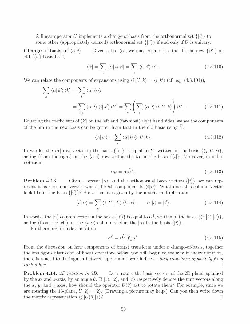
A linear operator U implements a change-of-basis from the orthonormal set |i〉 tosome other (appropriately defined) orthonormal set |i′〉 if and only if U is unitary.

Change-of-basis of 〈α| i〉 Given a bra 〈α|, we may expand it either in the new 〈i′| orold 〈i| basis bras,

〈α| =∑

i

〈α| i〉 〈i| =∑

i

〈α| i′〉 〈i′| . (4.3.110)

We can relate the components of expansions using 〈i |U | k〉 = 〈i| k′〉 (cf. eq. (4.3.101)),∑

k

〈α| k′〉 〈k′| =∑

i

〈α| i〉 〈i|

=∑

i,k

〈α| i〉 〈i| k′〉 〈k′| =∑

k

(∑

i

〈α| i〉 〈i |U | k〉)〈k′| . (4.3.111)

Equating the coefficients of 〈k′| on the left and (far-most) right hand sides, we see the components

of the bra in the new basis can be gotten from that in the old basis using U ,

〈α| k′〉 =∑

i

〈α| i〉 〈i |U | k〉 . (4.3.112)

In words: the 〈α| row vector in the basis 〈i′| is equal to U , written in the basis 〈j |U | i〉,acting (from the right) on the 〈α| i〉 row vector, the 〈α| in the basis 〈i|. Moreover, in indexnotation,

αk′ = αiUik. (4.3.113)

Problem 4.13. Given a vector |α〉, and the orthonormal basis vectors |i〉, we can rep-resent it as a column vector, where the ith component is 〈i|α〉. What does this column vectorlook like in the basis |i′〉? Show that it is given by the matrix multiplication

〈i′|α〉 =∑

k

⟨i∣∣U †∣∣ k⟩〈k|α〉 , U |i〉 = |i′〉 . (4.3.114)

In words: the |α〉 column vector in the basis |i′〉 is equal to U †, written in the basis ⟨j∣∣U †∣∣ i⟩,

acting (from the left) on the 〈i|α〉 column vector, the |α〉 in the basis |i〉.Furthermore, in index notation,

αi′ = (U †)ikαk. (4.3.115)

From the discussion on how components of bra(s) transform under a change-of-basis, togetherthe analogous discussion of linear operators below, you will begin to see why in index notation,there is a need to distinguish between upper and lower indices – they transform oppositely fromeach other.

Problem 4.14. 2D rotation in 3D. Let’s rotate the basis vectors of the 2D plane, spannedby the x- and z-axis, by an angle θ. If |1〉, |2〉, and |3〉 respectively denote the unit vectors alongthe x, y, and z axes, how should the operator U(θ) act to rotate them? For example, since weare rotating the 13-plane, U |2〉 = |2〉. (Drawing a picture may help.) Can you then write downthe matrix representation 〈j |U(θ)| i〉?

50

Change-of-basis of 〈i |X| j〉 Now we shall proceed to ask, how do we use U to change thematrix representation of some linear operator X written in the basis |i〉 to one in the basis|i〉′? Starting from 〈i′ |X| j′〉 we insert the completeness relation eq. (4.3.18) in the basis |i〉,on both the left and the right,

〈i′ |X| j′〉 =∑

k,l

〈i′| k〉 〈k |X| l〉 〈l| j′〉

=∑

k,l

⟨i∣∣U †∣∣ k⟩〈k |X| l〉 〈l |U | j〉 =

⟨i∣∣U †XU

∣∣ j⟩, (4.3.116)

where we have recognized (from equations (4.3.101) and (4.3.102)) 〈i′| k〉 =⟨i∣∣U †∣∣ k⟩and

〈l| j′〉 = 〈l |U | j〉. If we denote X ′ as the matrix representation of X with respect to the primed

basis; and X and U as their corresponding operators with respect to the unprimed basis, werecover the similarity transformation

X ′ = U †XU . (4.3.117)

In index notation, with primes on the indices reminding us that the matrix is written in theprimed basis |i′〉 and the unprimed indices in the unprimed basis |i〉,

X i′j′ = (U †)ikX

klU

lj . (4.3.118)

As already alluded to, we see here the i and j indices transform “oppositely” from each other – sothat, even in matrix algebra, if we view square matrices as (representations of) linear operatorsacting on some vector space, then the row index i should have a different position from thecolumn index j so as to distinguish their transformation properties. This will allow us to readilyimplement that fact, when upper and lower indices are repeated, the pair transform as a scalar– for example, X i′

i′ = X ii.14

On the other hand, from the last equality of eq. (4.3.116), we may also view X ′ as the matrixrepresentation of the operator

X ′ ≡ U †XU (4.3.119)

written in the old basis |i〉. To reiterate,

〈i′ |X| j′〉 =⟨i∣∣U †XU

∣∣ j⟩. (4.3.120)

The next two theorems can be interpreted as telling us that the Hermitian/unitary nature ofoperators and their spectra are really basis-independent constructs.

Theorem Let X ′ ≡ U †XU . If U is a unitary operator, X and X ′ shares thesame spectrum.

14This issue of upper versus lower indices will also appear in differential geometry. Given a pair of indices thattransform oppositely from each other, we want them to be placed differently (upper vs. lower), so that when weset their labels equal – with Einstein summation in force – they automatically transforms as a scalar, since thepair of transformations will undo each other.

51

Proof Let |λ〉 be the eigenvector and λ be the corresponding eigenvalue of X .

X |λ〉 = λ |λ〉 (4.3.121)

By inserting a I = U †U and multiplying both sides on the left by U †,

U †XUU † |λ〉 = λU † |λ〉 , (4.3.122)

X ′(U † |λ〉) = λ(U † |λ〉). (4.3.123)

That is, given the eigenvector |λ〉 of X with eigenvalue λ, the corresponding eigenvector of X ′

is U † |λ〉 with precisely the same eigenvalue λ.

Theorem. Let X ′ ≡ U †XU . If X is Hermitian, so is X ′. If X is unitary, sois X ′.

Proof If X is Hermitian, we consider X ′†.

X ′† =(U †XU

)†= U †X†(U †)† = U †XU = X ′. (4.3.124)

If X is unitary we consider X ′†X ′.

X ′†X ′ =(U †XU

)†(U †XU) = U †X†UU †XU = U †X†XU = U †U = I. (4.3.125)

Remark We won’t prove it here, but it is possible to find a unitary operator U , related torotation in R3, that relates any one of the Pauli operators to the other

U †σiU = σj, i 6= j. (4.3.126)

This is consistent with what we have already seen earlier, that all the σk have the samespectrum −1,+1.

Physical Significance To put the significance of these statements in a physical context,recall the eigenvalues of an observable are possible outcomes of a physical experiment, while Udescribes a change of basis. Just as classical observables such as lengths, velocity, etc. should notdepend on the coordinate system we use to compute the predictions of the underlying theory –in the discussion of curved space(time)s we will see the analogy there is called general covariance– we see here that the possible experimental outcomes from a quantum system is independent ofthe choice of basis vectors we use to predict them. Also notice the very Hermitian and Unitarynature of a linear operator is invariant under a change of basis.

Diagonalization of observable Diagonalization of a matrix is nothing but the change-of-basis, expressing a linear operator X in some orthonormal basis |i〉 to one where it becomesa diagonal matrix with respect to the orthonormal eigenket basis |λ〉. That is, suppose youstarted with

X =∑

k

λk |λk〉 〈λk| (4.3.127)

and defined the unitary operator

U |k〉 = |λk〉 ⇔ 〈i |U | k〉 = 〈i|λk〉 . (4.3.128)

52

Notice the kth column of U ik ≡ 〈i |U | k〉 are the components of the kth unit norm eigenvector

|λk〉 written in the |i〉 basis. This implies, via two insertions of the completeness relation ineq. (4.3.18),

X =∑

i,j,k

λk |i〉 〈i| λk〉 〈λk| j〉 〈j| . (4.3.129)

Taking matrix elements,

〈i |X| j〉 = X ij =

∑

k,l

〈i|λk〉λkδkl 〈λl| j〉 =∑

k,l

U ikλkδ

kl (U

†)lj . (4.3.130)

Multiplying both sides by U † on the left and U on the right, we have

U †XU = diag(λ1, λ2, . . . , λD). (4.3.131)

Schur decomposition. Not all linear operators are diagonalizable. However, we already knowthat any square matrix X can be brought to an upper triangular form

U †XU = Γ + N , Γ ≡ diag (λ1, . . . , λD) , (4.3.132)

where the λi are the eigenvalues of X and N is strictly upper triangular. We may now phrase

the Schur decomposition as a change-of-basis from X to its upper triangular form.

Given a linear operator X , it is always possible to find an orthonormal basis suchthat its matrix representation is upper triangular, with its eigenvalues forming itsdiagonal elements.

Trace Define the trace of a linear operator X as

Tr [X ] =∑

i

〈i |X| i〉 , 〈i| j〉 = δij . (4.3.133)

The Trace yields a complex number. Let us see that this definition is independent of theorthonormal basis |i〉. Suppose we found a different set of orthonormal basis |i′〉, with〈i′| j′〉 = δij. Now consider

∑

i

〈i′ |X| i′〉 =∑

i,j,k

〈i′| j〉 〈j |X| k〉 〈k| i′〉 =∑

i,j,k

〈k| i′〉 〈i′| j〉 〈j |X| k〉

=∑

j,k

〈k| j〉 〈j |X| k〉 =∑

k

〈k |X| k〉 . (4.3.134)

Because Tr is invariant under a change of basis, we can view the trace operation that turnsan operator into a genuine scalar. This notion of a scalar is analogous to the quantities (pres-sure of a gas, temperature, etc.) that do not change no matter what coordinates one uses tocompute/measure them.

53

Problem 4.15. Prove the following statements. For linear operators X and Y ,

Tr [XY ] = Tr [Y X ] (4.3.135)

Tr[U †XU

]= Tr [X ] (4.3.136)

Problem 4.16. Find the unit norm eigenvectors that can be expressed as a linear combi-nation of |1〉 and |2〉, and their corresponding eigenvalues, of the operator

X ≡ a (|1〉 〈1| − |2〉 〈2|+ |1〉 〈2|+ |2〉 〈1|) . (4.3.137)

Assume that |1〉 and |2〉 are orthogonal and of unit norm. (Hint: First calculate the matrix〈j |X| i〉.)

Now consider the operators built out of the orthonormal basis vectors |i〉 |i = 1, 2, 3.

Y ≡ a (|1〉 〈1| − |2〉 〈2| − |3〉 〈3|) , (4.3.138)

Z ≡ b |1〉 〈1| − ib |2〉 〈3|+ ib |3〉 〈2| .

(In equations (4.3.137) and (4.3.138), a and b are real numbers.) Are Y and Z hermitian? Writedown their matrix representations. Verify [Y, Z] = 0 and proceed to simultaneously diagonalizeY and Z.

Problem 4.17. Pauli matrices re-visited. Refer to the Pauli matrices σµ defined in eq.(8.1.26). Let pµ be a 4-component collection of real numbers. We may then view pµσ

µ (where µsums over 0 through 3) as a Hermitian operator acting on a 2 dimensional vector space.

1. Find the eigenvalues λ± and corresponding unit norm eigenvectors ξ± of piσi (where i sums

over 1 through 3). These are called the helicity eigenstates. Are they also eigenstates ofpµσ

µ? (Hint: consider [piσi, pµσ

µ].)

2. Explain why

piσi = λ+ξ

+(ξ+)† + λ−ξ−(ξ−)†. (4.3.139)

Can you write down the analogous expansion for pµσµ?

3. If we define the square root of an operator or matrix√A as the solution to

√A√A = A,

write down the expansion for√pµσµ.

4. These 2 component spinors ξ± play a key role in the study of Lorentz symmetry in 4 space-time dimensions. Consider applying an invertible transformation L B

A on these spinors, i.e.,replace

(ξ±)A → L BA (ξ±)B. (4.3.140)

(The A and B indices run from 1 to 2, the components of ξ±.) How does pµσµ change

under such a transformation? And, how does its determinant change?

54

Problem 4.18. Schrodinger’s equation The primary equation in quantum mechanics(and quantum field theory), governing how states evolve in time, is

i~∂t |ψ(t)〉 = H |ψ(t)〉 , (4.3.141)

where ~ ≈ 1.054572 × 10−34 J s is the reduced Planck’s constant, and H is the Hamiltonian(≡ Hermitian total energy linear operator) of the system. The physics of a particular system isencoded within H .

Suppose H is independent of time, and suppose its orthonormal eigenkets |Ei;nj〉 areknown (nj being the degeneracy label, running over all eigenkets with the same energy Ej), withH |Ei;ni〉 = Ei |Ei;ni〉 and Ei ∈ R, where we will assume the energies are discrete. Show thatthe solution to Schrodinger’s equation in (4.3.141) is

|ψ(t)〉 =∑

j,nj

e−(i/~)Ejt |Ej ;nj〉 〈Ej ;nj|ψ(t = 0)〉 , (4.3.142)

where |ψ(t = 0)〉 is the initial condition, i.e., the state |ψ(t)〉 at t = 0. (Hint: Check that eq.(4.3.141) and the initial condition are satisfied.) Since the initial state was arbitrary, what youhave verified is that the operator

U(t, t′) ≡∑

j,nj

e−(i/~)Ej(t−t′) |Ej ;nj〉 〈Ej ;nj| (4.3.143)

obeys Schrodinger’s equation,

i~∂tU(t, t′) = HU(t, t′). (4.3.144)

Is U(t, t′) unitary? Explain what is the operator U(t = t′)?Express the expectation value 〈ψ(t) |H|ψ(t)〉 in terms of the energy eigenkets and eigenvalues.

Compare it with the expectation value 〈ψ(t = 0) |H|ψ(t = 0)〉.What if the Hamiltonian in Schrodinger’s equation depends on time – what is the corre-

sponding U? Consider the following (somewhat formal) solution for U .

U(t, t′) ≡ I− i

~

∫ t

t′dτ1H(τ1) +

(− i

~

)2 ∫ t

t′dτ2

∫ τ2

t′dτ1H(τ2)H(τ1) + . . . (4.3.145)

= I+

∞∑

ℓ=1

Iℓ(t, t′), (4.3.146)

where the ℓ-nested integral Iℓ(t, t′) is

Iℓ(t, t′) ≡

(− i

~

)ℓ ∫ t

t′dτℓ

∫ τℓ

t′dτℓ−1· · ·

∫ τ3

t′dτ2

∫ τ2

t′dτ1H(τℓ)H(τℓ−1) . . .H(τ2)H(τ1). (4.3.147)

(Be aware that, if the Hamiltonian H(t) depends on time, it may not commute with itself atdifferent times, namely one cannot assume [H(τ1), H(τ2)] = 0 if τ1 6= τ2.) Verify that, for t > t′,

i~∂tU(t, t′) = H(t)U(t, t′). (4.3.148)

55

What is U(t = t′)? You should be able to conclude that |ψ(t)〉 = U(t, t′) |ψ(t′)〉. Hint: Startwith i~∂tIℓ(t, t

′) and employ Leibniz’s rule:

d

dt

(∫ β(t)

α(t)

F (t, z)dz

)=

∫ β(t)

α(t)

∂F (t, z)

∂tdz + F (t, β(t))β ′(t)− F (t, α(t))α′(t). (4.3.149)

Bonus: Can you prove Leibniz’s rule, by say, using the limit definition of the derivative?

4.4 Tensor Products of Vector Spaces

In this section we will introduce the concept of a tensor product. It is a way to “multiply” vectorspaces, through the product ⊗, to form a larger vector space. Tensor products not only arise inquantum theory but is present even in classical electrodynamics, gravitation and field theories ofnon-Abelian gauge fields interacting with spin−1/2 matter. In particular, tensor products arisein quantum theory when you need to, for example, describe both the spatial wave-function andthe spin of a particle.

Definition To set our notation, let us consider multiplying N ≥ 2 distinct vector spaces,i.e., V1 ⊗ V2 ⊗ · · · ⊗ VN to form a VL. We write the tensor product of a vector |α1; 1〉 from V1,|α2; 2〉 from V2 and so on through |αN ;N〉 from VN as

|A;L〉 ≡ |α1; 1〉 ⊗ |α2; 2〉 ⊗ · · · ⊗ |αN ;N〉 , (4.4.1)

where it is understood the vector |αi; i〉 in the ith slot (from the left) is an element of the ithvector space Vi. As we now see, the tensor product is multi-linear because it obeys the followingalgebraic rules.

1. The tensor product is distributive over addition. For example,

|α〉 ⊗ (|α′〉+ |β ′〉)⊗ |α′′〉 = |α〉 ⊗ |α′〉 ⊗ |α′′〉+ |α〉 ⊗ |β ′〉 ⊗ |α′′〉 . (4.4.2)

2. Scalar multiplication can be factored out. For example,

c (|α〉 ⊗ |α′〉) = (c |α〉)⊗ |α′〉 = |α〉 ⊗ (c |α′〉). (4.4.3)

Our larger vector space VL is spanned by all vectors of the form in eq. (4.4.1), meaning everyvector in VL can be expressed as a linear combination:

|A′;L〉 ≡∑

α1,...,αN

Cα1,...,αN |α1; 1〉 ⊗ |α2; 2〉 ⊗ · · · ⊗ |αN ;N〉 ∈ VL. (4.4.4)

(The Cα1,...,αN is just a collection complex numbers.) In fact, if we let |i; j〉 |i = 1, 2, . . . , Djbe the basis vectors of the jth vector space Vj ,

|A′;L〉 =∑

α1,...,αN

∑

i1,...,iN

Cα1,...,αN 〈i1; 1|α1〉 〈i2; 2|α2〉 . . . 〈iN ;N |αN〉

× |i1; 1〉 ⊗ |i2; 2〉 ⊗ · · · ⊗ |iN ;N〉 . (4.4.5)

56

In other words, the basis vectors of this tensor product space VL are formed from products ofthe basis vectors from each and every vector space Vi.

Dimension If the ith vector space Vi has dimension Di, then the dimension of VL itselfis D1D2 . . .DN−1DN . The reason is, for a given tensor product |i1; 1〉 ⊗ |i2; 2〉 ⊗ · · · ⊗ |iN ;N〉,there are D1 choices for |i1; 1〉, D2 choices for |i2; 2〉, and so on.

Example Suppose we tensor two copies of the 2-dimensional vector space that the Paulioperators σi act on. Each space is spanned by |±〉. The tensor product space is then spannedby the following 4 vectors

|1;L〉 = |+〉 ⊗ |+〉 , |2;L〉 = |+〉 ⊗ |−〉 , (4.4.6)

|3;L〉 = |−〉 ⊗ |+〉 , |4;L〉 = |−〉 ⊗ |−〉 . (4.4.7)

(Note that this ordering of the vectors is of course not unique.)Adjoint and Inner Product Just as we can form tensor products of kets, we can do

so for bras. We have

(|α1〉 ⊗ |α2〉 ⊗ · · · ⊗ |αN〉)† = 〈α1| ⊗ 〈α2| ⊗ · · · ⊗ 〈αN | , (4.4.8)

where the ith slot from the left is a bra from the ith vector space Vi. We also have the innerproduct

(〈α1| ⊗ 〈α2| ⊗ · · · ⊗ 〈αN |) (c |β1〉 ⊗ |β2〉 ⊗ · · · ⊗ |βN〉+ d |γ1〉 ⊗ |γ2〉 ⊗ · · · ⊗ |γN〉)= c 〈α1|β1〉 〈α2| β2〉 . . . 〈αN |βN〉+ d 〈α1| γ1〉 〈α2| γ2〉 . . . 〈αN | γN〉 , (4.4.9)

where c and d are complex numbers. For example, the orthonormal nature of the |i1; 1〉⊗ · · ·⊗|iN ;N〉 follow from

(〈j1; 1| ⊗ · · · ⊗ 〈jN ;N |) (|i1; 1〉 ⊗ · · · ⊗ |iN ;N〉) = 〈j1; 1| i1; 1〉 〈j2; 2| i2; 2〉 . . . 〈jN ;N | iN ;N〉= δj1i1 . . . δ

jNiN. (4.4.10)

Linear Operators If Xi is a linear operator acting on the ith vector space Vi, we can forma tensor product of them. Their operation is defined as

(X1 ⊗X2 ⊗ · · · ⊗XN) (c |β1〉 ⊗ |β2〉 ⊗ · · · ⊗ |βN〉+ d |γ1〉 ⊗ |γ2〉 ⊗ · · · ⊗ |γN〉) (4.4.11)

= c(X1 |β1〉)⊗ (X2 |β2〉)⊗ · · · ⊗ (XN |βN〉) + d(X1 |γ1〉)⊗ (X2 |γ2〉)⊗ · · · ⊗ (XN |γN〉),

where c and d are complex numbers.The most general linear operator Y acting on our tensor product space VL can be built out

of the basis ket-bra operators.

Y =∑

i1,...,iNj1,...,jN

(|i1; 1〉 ⊗ · · · ⊗ |iN ;N〉)Y i1...iNj1...jN

(〈j1; 1| ⊗ · · · ⊗ 〈jN ;N |) , (4.4.12)

Y i1...iNj1...jN

∈ C. (4.4.13)

Problem 4.19. Tensor transformations. Consider the state

|A′;L〉 =∑

1≤i1≤D1

∑

1≤i2≤D2

· · ·∑

1≤iN≤DN

T i1i2...iN−1iN |i1; 1〉 ⊗ |i2; 2〉 ⊗ · · · ⊗ |iN ;N〉 , (4.4.14)

57

where |ij ; j〉 are the Dj orthonormal basis vectors spanning the jth vector space Vj , andT i1i2...iN−1iN are complex numbers. Consider a change of basis for each vector space, i.e., |i; j〉 →|i′; j〉. By defining the unitary operator that implements this change-of-basis

U ≡ (1)U ⊗ (2)U ⊗ · · · ⊗ (N)U, (4.4.15)

(i)U ≡∑

1≤j≤Di

|j′; i〉 〈j; i| , (4.4.16)

expand |A′;L〉 in the new basis |j′1; 1〉 ⊗ · · · ⊗ |j′N ;N〉; this will necessarily involve the U †’s.Define the coefficients of this new basis via

|A′;L〉 =∑

1≤i′1≤D1

∑

1≤i′2≤D2

· · ·∑

1≤i′N≤DN

T ′i′1i′2...i

′N−1i

′N |i′1; 1〉 ⊗ |i′2; 2〉 ⊗ · · · ⊗ |i′N ;N〉 . (4.4.17)

Now relate T ′i′1i′2...i

′N−1i

′N to the coefficients in the old basis T i1i2...iN−1iN using the matrix elements

((i)U

†)j

k≡⟨j; i∣∣∣((i)U

)†∣∣∣ k; i⟩. (4.4.18)

Can you perform a similar change-of-basis for the following dual vector?

〈A′;L| =∑

1≤i1≤D1

∑

1≤i2≤D2

· · ·∑

1≤iN≤DN

Ti1i2...iN−1iN 〈i1; 1| ⊗ 〈i2; 2| ⊗ · · · ⊗ 〈iN ;N | (4.4.19)

In differential geometry, tensors will transform in analogous ways.

4.5 Continuous Spaces and Infinite D−Space

For the final section we will deal with vector spaces with continuous spectra, with infinite di-mensionality. To make this topic rigorous is beyond the scope of these notes; but the interestedreader should consult the functional analysis portion of the math literature. Our goal here is apractical one: we want to be comfortable enough with continuous spaces to solve problems inquantum mechanics and (quantum and classical) field theory.

4.5.1 Preliminaries: Dirac’s δ and eigenket integrals

Dirac’s δ-“function” We will see that transitioning from discrete, finite dimensional vec-tor spaces to continuous ones means summations become integrals; while Kronecker-δs will bereplaced with Dirac-δ functions. In case the latter is not familiar, the Dirac-δ function of onevariable is to be viewed as an object that occurs within an integral, and is defined via

∫ b

a

f(x′)δ(x′ − x)dx′ = f(x), (4.5.1)

for all a less than x and all b greater than x, i.e., a < x < b. This indicates δ(x′ − x) has to besharply peaked at x′ = x and zero everywhere, since the result of integral picks out the value off solely at x.

58

The Dirac δ-function is often loosely viewed as δ(x) = 0 when x 6= 0 and δ(x) = ∞ whenx = 0. An alternate approach is to define δ(x) as a sequence of functions more and more sharplypeaked at x = 0, whose integral over the real line is unity. Three examples are

δ(x) = limǫ→0+

Θ( ǫ2− |x|

) 1

ǫ(4.5.2)

= limǫ→0+

e−|x|ǫ

2ǫ(4.5.3)

= limǫ→0+

1

π

ǫ

x2 + ǫ2(4.5.4)

For the first equality, Θ(z) is the step function, defined to be

Θ(z) = 1, for z > 0

= 0, for z < 0. (4.5.5)

Problem 4.20. Justify these three definitions of δ(x). What happens, for finite x 6= 0,when ǫ → 0+? Then, by holding ǫ fixed, integrate them over the real line, before proceeding toset ǫ→ 0+.

For later use, we record the following integral representation of the Dirac δ-function.

∫ +∞

−∞

dω

2πeiω(z−z′) = δ(z − z′) (4.5.6)

Problem 4.21. Can you justify the following?

Θ(z − z′) =

∫ z

z0

dz′′δ(z′′ − z′), z′ > z0. (4.5.7)

We may therefore assert the derivative of the step function is the δ-function,

Θ′(z − z′) = δ(z − z′). (4.5.8)

A few properties of the δ-function are worth highlighting.

• From eq. (4.5.8) – that a δ(z − z′) follows from taking the derivative of a discontinuousfunction – in this case, Θ(z − z′) – will be important for the study of Green’s functions.

• If the argument of the δ-function is a function f of some variable z, then as long as f ′(z) 6= 0whenever f(z) = 0, it may be re-written as

δ (f(z)) =∑

zi≡ith zero of f(z)

δ(z − zi)

|f ′(zi)|. (4.5.9)

59

To justify this we recall the fact that, the δ-function itself is non-zero only when its argu-ment is zero. This explains why we sum over the zeros of f(z). Now we need to fix thecoefficient of the δ-function near each zero. That is, what are the ϕi’s in

δ (f(z)) =∑

zi≡ith zero of f(z)

δ(z − zi)

ϕi? (4.5.10)

We now use the fact that integrating a δ-function around the small neighborhood of the ithzero of f(z) with respect to f has to yield unity. It makes sense to treat f as an integrationvariable near its zero because we have assumed its slope is non-zero, and therefore near itsith zero,

f(z) = f ′(zi)(z − zi) +O((z − zi)2), (4.5.11)

⇒ df = f ′(zi)dz +O((z − zi)1)dz. (4.5.12)

The integration around the ith zero reads, for 0 < ǫ≪ 1,

1 =

∫ z=zi+ǫ

z=zi−ǫ

dfδ (f) =

∫ z=zi+ǫ

z=zi−ǫ

dz∣∣(f ′(zi) +O((z − zi)

1))∣∣ δ (z − zi)

ϕi

(4.5.13)

ǫ→0→ |f ′(zi)|ϕi

. (4.5.14)

(When you change variables within an integral, remember to include the absolute value ofthe Jacobian, which is essentially |f ′(zi)| in this case.) The O(zp) means “the next termin the series has a dependence on the variable z that goes as zp”; this first correction canbe multiplied by other stuff, but has to be proportional to zp.

A simple application of eq. (4.5.9) is, for a ∈ R,

δ(az) =δ(z)

|a| . (4.5.15)

• Since δ(z) is non-zero only when z = 0, it must be that δ(−z) = δ(z) and more generally

δ(z − z′) = δ(z′ − z). (4.5.16)

• We may also take the derivative of a δ-function. Under an integral sign, we may applyintegration-by-parts as follows:

∫ b

a

δ′(x− x′)f(x)dx = [δ(x− x′)f(x)]x=bx=a −

∫ b

a

δ(x− x′)f ′(x)dx = −f ′(x′) (4.5.17)

as long as x′ lies strictly between a and b, a < x′ < b, where a and b are both real.

• Dimension What is the dimension of the δ-function? Turns out δ(ξ) has dimensionsof 1/[ξ], i.e., the reciprocal of the dimension of its argument. The reason is

∫dξδ(ξ) = 1 ⇒ [ξ] [δ(ξ)] = 1. (4.5.18)

60

Continuous spectrum Let Ω be a Hermitian operator whose spectrum is continuous;i.e., Ω |ω〉 = ω |ω〉 with ω being a continuous parameter. If |ω〉 and |ω′〉 are both “unit norm”eigenvectors of different eigenvalues ω and ω′, we have

〈ω|ω′〉 = δ(ω − ω′). (4.5.19)

(This assumes a “translation symmetry” in this ω-space; we will see later how to modify thisinner product when the translation symmetry is lost.) The completeness relation in eq. (4.3.18)is given by

∫dω |ω〉 〈ω| = I. (4.5.20)

An arbitrary vector |α〉 can be expressed as

|α〉 =∫

dω |ω〉 〈ω|α〉 . (4.5.21)

When the state is normalized to unity, we say

〈α|α〉 =∫

dω 〈α|ω〉 〈ω|α〉 =∫

dω| 〈ω|α〉 |2 = 1. (4.5.22)

The inner product between arbitrary vectors |α〉 and |β〉 now reads

〈α|β〉 =∫

dω 〈α|ω〉 〈ω|β〉 . (4.5.23)

Since by assumption Ω is diagonal, i.e.,

Ω =

∫dωω |ω〉 〈ω| , (4.5.24)

the matrix elements of Ω are

〈ω |Ω|ω′〉 = ωδ(ω − ω′) = ω′δ(ω − ω′). (4.5.25)

Because of the δ-function, it does not matter if we write ω or ω′ on the right hand side.

4.5.2 Continuous Operators, Translations, and the Fourier transform

An important example that we will deal in detail here, is that of the eigenket of the positionoperator ~X, where we assume there is some underlying infinite D-space RD. The arrow indicatesthe position operator itself has D components, each one corresponding to a distinct axis of theD-dimensional Euclidean space. |~x〉 would describe the state that is (infinitely) sharply localizedat the position ~x; namely, it obeys the D-component equation

~X |~x〉 = ~x |~x〉 . (4.5.26)

61

Or, in index notation,

Xk |~x〉 = xk |~x〉 , k ∈ 1, 2, . . . , D. (4.5.27)

The position eigenkets are normalized as, in Cartesian coordinates,

〈~x| ~x′〉 = δ(D)(~x− ~x′) ≡D∏

i=1

δ(xi − x′i) = δ(x1 − x′1)δ(x2 − x′2) . . . δ(xD − x′D). (4.5.28)

15Any other vector |α〉 in the Hilbert space can be expanded in terms of the position eigenkets.

|α〉 =∫

RD

dD~x |~x〉 〈~x|α〉 . (4.5.31)

Notice 〈~x|α〉 is an ordinary (possibly complex) function of the spatial coordinates ~x. We seethat the space of functions emerges from the vector space spanned by the position eigenkets.Just as we can view 〈i|α〉 in |α〉 =

∑i |i〉 〈i|α〉 as a column vector, the function f(~x) ≡ 〈~x| f〉

is in some sense a continuous (infinite dimensional) “vector” in this position representation.In the context of quantum mechanics 〈~x|α〉 would be identified as a wave function, more

commonly denoted as ψ(~x); in particular, | 〈~x|α〉 |2 is interpreted as the probability density thatthe system is localized around ~x when its position is measured. This is in turn related to thedemand that the wave function obey

∫dD~x| 〈~x|α〉 |2 = 1. However, it is worth highlighting here

that our discussion regarding the Hilbert spaces spanned by the position eigenkets |~x〉 (and

later below, by their momentum counterparts |~k〉) does not necessarily have to involve quantumtheory.16 We will provide concrete examples below, such as how the concept of Fourier transformemerges and how classical field theory problems – the derivation of the Green’s function of theLaplacian in eq. (9.3.48), for instance – can be tackled using the methods/formalism delineatedhere.

15As an important aside, the generalization of the 1D transformation law in eq. (4.5.9) involving the δ-functionhas the following higher dimensional generalization. If we are given a transformation ~x ≡ ~x(~y) and ~x′ ≡ ~x′(~y′),then

δ(D) (~x− ~x′) =δ(D)(~y − ~y′)

|det ∂xa(~y)/∂yb| =δ(D)(~y − ~y′)

|det ∂x′a(~y′)/∂y′b| , (4.5.29)

where δ(D)(~x − ~x′) ≡ ∏Di=1 δ(x

i − x′i), δ(D)(~y − ~y′) ≡ ∏Di=1 δ(y

i − y′i), and the Jacobian inside the absolutevalue occurring in the denominator on the right hand side is the usual determinant of the matrix whose ath rowand bth column is given by ∂xa(~y)/∂yb. (The second and third equalities follow from each other because theδ-functions allow us to assume ~y = ~y′.) Equation (4.5.29) can be justified by demanding that its integral aroundthe point ~x = ~x′ gives one. For 0 < ǫ≪ 1, and denoting δ(D)(~x− ~x′) = δ(D)(~y − ~y′)/ϕ(~y′),

1 =

∫

|~x−~x′|≤ǫ

dD~xδ(D)(~x− ~x′) =

∫

|~x−~x′|≤ǫ

dD~y

∣∣∣∣det∂xa(~y)

∂yb

∣∣∣∣δ(D)(~y − ~y′)

ϕ(~y′)=

∣∣∣det ∂x′a(~y′)∂y′b

∣∣∣ϕ(~y′)

. (4.5.30)

16This is especially pertinent for those whose first contact with continuous Hilbert spaces was in the contextof a quantum mechanics course.

62

Matrix elements Suppose we wish to calculate the matrix element 〈α |Y |β〉 in theposition representation. It is

〈α |Y |β〉 =∫

dD~x

∫dD~x′ 〈α|~x〉 〈~x |Y | ~x′〉 〈~x′|β〉

=

∫dD~x

∫dD~x′ 〈~x|α〉∗ 〈~x |Y |~x′〉 〈~x′| β〉 . (4.5.32)

If the operator Y ( ~X) were built solely from the position operator ~X, then

⟨~x∣∣∣Y ( ~X)

∣∣∣ ~x′⟩= Y (~x)δ(D)(~x− ~x′) = Y (~x′)δ(D)(~x− ~x′); (4.5.33)

and the double integral collapses into one,

⟨α∣∣∣Y ( ~X)

∣∣∣ β⟩=

∫dD~x 〈~x|α〉∗ 〈~x′| β〉Y (~x). (4.5.34)

Problem 4.22. Show that if U is a unitary operator and |α〉 is an arbitrary vector, then|α〉, U |α〉 and U † |α〉 have the same norm.

Continuous unitary operators Translations and rotation are examples of operationsthat involve continuous parameter(s) – for translation it involves a displacement vector; forrotation we have to specify the axis of rotation as well as the angle of rotation itself.

Exp(anti-Hermitian operator) is unitary It will often be the case that, whenrealized as linear operators on some Hilbert space, these continuous operators willbe unitary. Suppose further, when their parameters ~ξ – which we will assume to bereal – are tuned to zero ~0, the identity operator is recovered. When these conditionsare satisfied, the continuous unitary operator U can (in most cases of interest) be

expressed as the exponential of the anti-Hermitian operator −i~ξ · ~K, namely

U(~ξ) = exp(−i~ξ · ~K

). (4.5.35)

To be clear, we are allowing for N ≥ 1 continuous real parameter(s), which we collectively denote

as ~ξ. The Hermitian operator will also have N distinct components, so ~ξ · ~K ≡∑

i ξiKi.

To check the unitary nature of eq. (4.5.35), we first record that the exponential of an operatorX is defined through the Taylor series

eX ≡ I+X +X2

2!+X3

3!+ · · · =

∞∑

ℓ=0

Xℓ

ℓ!. (4.5.36)

For X = −i~ξ · ~K, where ~ξ is real and ~K is Hermitian, we have

X† =(−i~ξ · ~K

)†= i~ξ · ~K† = i~ξ · ~K = −X. (4.5.37)

63

That is, X is anti-Hermitian. Now, for ℓ integer, (Xℓ)† = (X†)ℓ = (−X)ℓ. Thus,

(eX)† =∞∑

ℓ=0

(Xℓ)†

ℓ!=

∞∑

ℓ=0

(−X)ℓ

ℓ!= e−X . (4.5.38)

Generically, operators do not commute AB 6= BA. (Such a non-commuting example is rota-tion.) In that case, exp(A + B) 6= exp(A) exp(B). However, because X and −X do commute,we can check the unitary nature of expX by Taylor expanding each of the exponentials inexp(X)(exp(X))† = exp(X) exp(−X) and finding that the series can be re-arranged to that ofexp(X −X) = I. Specifically, whenever A and B do commute

exp(A) exp(B) =∞∑

ℓ1,ℓ2=0

Aℓ1Bℓ2

ℓ1!ℓ2!=

∞∑

ℓ=0

1

ℓ!

ℓ∑

s=0

(ℓ

s

)AsBℓ−s (4.5.39)

=

∞∑

ℓ=0

(A+B)ℓ

ℓ!= exp(A+B). (4.5.40)

Translation in RD To make these ideas regarding continuous operators more concrete, wewill now study the case of translation in some detail, realized on a Hilbert space spanned by theposition eigenkets |~x〉. To be specific, let T (~d) denote the translation operator parameterized

by the displacement vector ~d. We shall work in D space dimensions. We define the translationoperator by its action

T (~d) |~x〉 =∣∣∣~x+ ~d

⟩. (4.5.41)

Since |~x〉 and |~x + ~d〉 can be viewed as distinct elements of the set of basis vectors, we shallsee that the translation operator can be viewed as a unitary operator, changing basis from|~x〉 |~x ∈ RD to |~x+ ~d〉|~x ∈ RD. The inverse transformation is

T (~d)† |~x〉 =∣∣∣~x− ~d

⟩. (4.5.42)

Of course we have the identity operator I when ~d = ~0,

T (~0) |~x〉 = |~x〉 ⇒ T (~0) = I. (4.5.43)

The following composition law has to hold

T (~d1)T (~d2) = T (~d1 + ~d2), (4.5.44)

because translation is commutative

T (~d1)T (~d2) |~x〉 = T (~d1)∣∣∣~x+ ~d2

⟩=∣∣∣~x+ ~d2 + ~d1

⟩=∣∣∣~x+ ~d1 + ~d2

⟩= T (~d1 + ~d2) |~x〉 . (4.5.45)

Problem 4.23. Translation operator is unitary. Show that

T (~d) =

∫

RD

dD~x′∣∣∣~d+ ~x′

⟩〈~x′| (4.5.46)

satisfies eq. (4.5.41) and therefore is the correct ket-bra operator representation of the translation

operator. Check explicitly that T (~d) is unitary.

64

Momentum operator Since eq. (4.5.46) tells us the translation operator is unitary, wemay now invoke the form of the continuous unitary operator in eq. (4.5.35) to deduce

T (~ξ) = exp(−i~ξ · ~P

)= exp

(−iξkPk

)(4.5.47)

We will call the Hermitian operator ~P the momentum operator.17 In this exp form, eq. (4.5.44)reads

exp(−i~d1 · ~P

)exp

(−i~d2 · ~P

)= exp

(−i(~d1 + ~d2) · ~P

). (4.5.48)

Translation invariance Infinite (flat) D-space RD is the same everywhere and in every di-

rection. This intuitive fact is intimately tied to the property that T (~d) is a unitary operator: itjust changes one orthonormal basis to another, and physically speaking, there is no privilegedset of basis vectors. For instance, the norm of vectors is position independent:

⟨~x+ ~d

∣∣∣ ~x′ + ~d⟩= δ(D) (~x− ~x′) = 〈~x|~x′〉 . (4.5.49)

As we will see below, if we confine our attention to some finite domain in RD or if space is nolonger flat, then (global) translation symmetry is lost and the translation operator still existsbut is no longer unitary.18 In particular, when the domain is finite eq. (4.5.46) may no longermake sense; a 1D example would be to consider |z〉 |0 ≤ z ≤ L,

T (d > 0)?=

∫ L

0

dz′ |z′ + d〉 〈z′| . (4.5.50)

When z′ = L, say, the bra in the integrand is 〈L| but the ket |L+ d〉 would make no sensebecause L+ d lies outside the domain.

Commutation relations between X i and Pj We have seen, just from postulating a Hermi-tian position operator X i, and considering the translation operator acting on the space spannedby its eigenkets |~x〉, that there exists a Hermitian momentum operator Pj that occurs in theexponent of said translation operator. This implies the continuous space at hand can be spannedby either the position eigenkets |~x〉 or the momentum eigenkets, which obey

Pj |~k〉 = kj|~k〉. (4.5.51)

Are the position and momentum operators simultaneously diagonalizable? Can we label a statewith both position and momentum? The answer is no.

To see this, we now consider an infinitesimal displacement operator T (d~ξ).

~XT (d~ξ) |~x〉 = ~X∣∣∣~x+ d~ξ

⟩= (~x+ d~ξ)

∣∣∣~x+ d~ξ⟩, (4.5.52)

17Strictly speaking Pj here has dimensions of 1/[length], whereas the momentum you might be familiar withhas units of [mass × length/time2].

18When we restrict the domain to a finite one embedded within flat RD, there is still local translation symmetryin that, performing the same experiment at ~x and at ~x′ should not lead to any physical differences as long as

both ~x and ~x′ lie within the said domain. But global translation symmetry is “broken” because, the domain is“here” and not “there”; as illustrated by the 1D example, translating too much in one direction would bring youout of the domain.

65

and

T (d~ξ) ~X |~x〉 = ~x∣∣∣~x+ d~ξ

⟩. (4.5.53)

Since |~x〉 was an arbitrary vector, we may subtract the two equations

[~X, T (d~ξ)

]|~x〉 = d~ξ

∣∣∣~x+ d~ξ⟩= d~ξ |~x〉+O

(d~ξ2). (4.5.54)

At first order in d~ξ, we have the operator identity

[~X, T (d~ξ)

]= d~ξ. (4.5.55)

The left hand side involves operators, but the right hand side only real numbers. At this pointwe invoke eq. (4.5.47), and deduce, for infinitesimal displacements,

T (d~ξ) = 1− id~ξ · ~P +O(d~ξ2) (4.5.56)

which in turn means eq. (4.5.55) now reads, as d~ξ → ~0,

[~X,−id~ξ · ~P

]= d~ξ (4.5.57)

[X l, Pj

]dξj = iδljdξ

j (the lth component) (4.5.58)

Since the dξj are independent, the coefficient of dξj on both sides must be equal. This leadsus to the fundamental commutation relation between kth component of the position operatorwith the j component of the momentum operator:

[Xk, Pj

]= iδkj , j, k ∈ 1, 2, . . . , D. (4.5.59)

To sum: although Xk and Pj are both Hermitian operators in infinite flat RD, we see theyare incompatible and thus, to span the continuous vector space at hand we can use either theeigenkets of X i or that of Pj but not both. We will, in fact, witness below how changing fromthe position to momentum eigenket basis gives rise to the Fourier transform and its inverse.

|f〉 =∫

RD

dD~x′ |~x′〉 〈~x′| f〉 , X i |~x′〉 = x′i |~x′〉 (4.5.60)

|f〉 =∫

RD

dD~k′∣∣∣~k′⟩ ⟨

~k′∣∣∣ f⟩, Pj

∣∣∣~k′⟩= k′j

∣∣∣~k′⟩. (4.5.61)

For those already familiar with quantum theory, notice there is no ~ on the right hand side;nor will there be any throughout this section. This is not because we have “set ~ = 1” as iscommonly done in theoretical physics literature. Rather, it is because we wish to reiterate thatthe linear algebra of continuous operators, just like its discrete finite dimension counterparts, isreally an independent structure on its own. Quantum theory is merely one of its application,albeit a very important one.

66

Problem 4.24. Because translation is commutative, ~d1 + ~d2 = ~d2 + ~d1, argue that thetranslation operators commute:

[T (~d1), T (~d2)

]= 0. (4.5.62)

By considering infinitesimal displacements ~d1 = d~ξ1 and ~d2 = d~ξ2, show that eq. (4.5.47) leadsto us to conclude that momentum operators commute among themselves,

[Pi, Pj] = 0, i, j ∈ 1, 2, 3, . . . , D. (4.5.63)

Problem 4.25. Let |~k〉 be an eigenket of the momentum operator ~P . Is |~k〉 an eigenvector

of T (~d)? If so, what is the corresponding eigenvalue?

Problem 4.26. Derive the momentum operator ~P in the position eigenket basis,

⟨~x∣∣∣ ~P∣∣∣α⟩= −i ∂

∂~x〈~x|α〉 , (4.5.64)

for an arbitrary state |α〉. Hint: begin with⟨~x∣∣∣T (d~ξ)

∣∣∣α⟩=⟨~x− d~ξ

∣∣∣α⟩. (4.5.65)

Taylor expand both the operator T (d~ξ) as well as the function⟨~x− d~ξ

∣∣∣α⟩, and take the d~ξ → ~0

limit, keeping only the O(d~ξ) terms.

Next, check that this representation of ~P is consistent with eq. (4.5.59) by considering⟨~x∣∣[Xk, Pj

]∣∣α⟩= iδkj 〈~x|α〉 . (4.5.66)

Start by expanding the commutator on the left hand side, and show that you can recover eq.(4.5.64).

Problem 4.27. Express the following matrix element in the position space representation

⟨α∣∣∣ ~P∣∣∣ β⟩=

∫dD~x

(?

). (4.5.67)

Problem 4.28. Show that the negative of the Laplacian, namely

−~∇2 ≡ −∑

i

∂

∂xi∂

∂xi(in Cartesian coordinates xi), (4.5.68)

is the square of the momentum operator. That is, for an arbitrary state |α〉, show that

⟨~x∣∣∣ ~P 2∣∣∣α⟩= −δij ∂

∂xi∂

∂xj〈~x|α〉 ≡ −~∇2 〈~x|α〉 . (4.5.69)

67

Problem 4.29. Translation as Taylor series. Use equations (4.5.47) and (4.5.64) to infer,for an arbitrary state |f〉,

⟨~x+ ~ξ

∣∣∣ f⟩= exp

(~ξ · ∂

∂~x

)〈~x| f〉 . (4.5.70)

Compare the right hand side with the Taylor expansion of the function f(~x+ ~ξ) about ~x.

Problem 4.30. Prove the Campbell-Baker-Hausdorff lemma. For linear operators A andB, and complex number α,

eiαABe−iαA =∞∑

ℓ=0

(iα)ℓ

ℓ![A, [A, . . . [A︸ ︷︷ ︸

ℓ of these

, B]]], (4.5.71)

where the ℓ = 0 term is understood to be just B. (Hint: Taylor expand the left-hand-side anduse mathematical induction.)

Next, consider the expectation values of the position ~X and momentum ~P operator withrespect to a general state |ψ〉:

⟨ψ∣∣∣ ~X∣∣∣ψ⟩

and⟨ψ∣∣∣ ~P∣∣∣ψ⟩. (4.5.72)

What happens to these expectation values when we replace |ψ〉 → T (~d) |ψ〉?(Lie) Group theory Our discussion here on the unitary operator T that implements

translations on the Hilbert space spanned by the position eigenkets |~x〉, is really an informalintroduction to the theory of continuous groups. The collection of continuous unitary transla-tion operators T (~d) forms a group, which like a vector space is defined by a set of axioms.Continuous unitary group elements that can be brought to the identity operator, by settingthe continuous real parameters to zero, can always be expressed in the exponential form in eq.(4.5.35). The Hermitian operators ~K, that is said to “generate” the group elements, may obeynon-trivial commutation relations (aka Lie algebra). For instance, because rotation operationsin Euclidean space do not commute – rotating about the z-axis followed by rotation about thex-axis, is not the same as rotation about the x-axis followed by about the z-axis – their corre-sponding unitary operators acting on the Hilbert space spanned by |~x〉 will give rise to, in 3dimensional space, [Ki, Kj] = iǫijlKl, for i, j, l ∈ 1, 2, 3.

Fourier analysis We will now show how the concept of a Fourier transform readilyarises from the formalism we have developed so far. To initiate the discussion we start with eq.(4.5.64), with |α〉 replaced with a momentum eigenket |~k〉. This yields the eigenvalue/vectorequation for the momentum operator in the position representation.

⟨~x∣∣∣~P∣∣∣~k⟩= ~k〈~x|~k〉 = −i ∂

∂~x〈~x|~k〉, ⇔ kj〈~x|~k〉 = −i∂〈~x|

~k〉∂xj

. (4.5.73)

In D-space, this is a set of D first order differential equations for the function 〈~x|~k〉. Via a directcalculation you can verify that the solution to eq. (4.5.73) is simply the plane wave

〈~x|~k〉 = χ exp(i~k · ~x

). (4.5.74)

68

where χ is complex constant to be fixed in the following way. We want∫

RD

dDk〈~x|~k〉〈~k|~x′〉 = 〈~x| ~x′〉 = δ(D)(~x− ~x′). (4.5.75)

Using the plane wave solution,

(2π)D|χ|2∫

dDk

(2π)Dei~k·(~x−~x′) = δ(D)(~x− ~x′). (4.5.76)

Now, recall the representation of the D-dimensional δ-function∫

RD

dDk

(2π)Dei~k·(~x−~x′) = δ(D)(~x− ~x′). (4.5.77)

Therefore, up to an overall multiplicative phase eiδ, which we will choose to be unity, χ =1/(2π)D/2 and eq. (4.5.74) becomes

〈~x|~k〉 = (2π)−D/2 exp(i~k · ~x

). (4.5.78)

By comparing eq. (4.5.78) with eq. (4.3.101), we see that the plane wave in eq. (4.5.78) canbe viewed as the matrix element of the unitary operator implementing the change-of-basis fromposition to momentum space, and vice versa.

We may now examine how the position representation of an arbitrary state 〈~x| f〉 can beexpanded in the momentum eigenbasis.

〈~x| f〉 =∫

RD

dD~k〈~x|~k〉⟨~k∣∣∣ f⟩=

∫

RD

dD~k

(2π)D/2ei~k·~x⟨~k∣∣∣ f⟩

(4.5.79)

Similarly, we may expand the momentum representation of an arbitrary state⟨~k∣∣∣ f⟩

in the

position eigenbasis.

⟨~k∣∣∣ f⟩=

∫

RD

dD~x⟨~k∣∣∣ ~x⟩〈~x| f〉 =

∫

RD

dD~x

(2π)D/2e−i~k·~x 〈~x| f〉 (4.5.80)

Equations (4.5.79) and (4.5.80) are nothing but the Fourier expansion of some function f(~x) andits inverse transform.19

Plane waves as orthonormal basis vectors For practical calculations, it is of course cum-bersome to carry around the position |~x〉 or momentum eigenkets |~k〉. As far as the space offunctions in RD is concerned, i.e., if one works solely in terms of the components f(~x) ≡ 〈~x| f〉,as opposed to the space spanned by |~x〉, then one can view the plane waves exp(i~k ·~x)/(2π)D/2in the Fourier expansion of eq. (4.5.79) as the orthonormal basis vectors. The coefficients of the

expansion are then the f(~k) ≡ 〈~k|f〉.

f(~x) =

∫

RD

dD~k

(2π)D/2ei~k·~xf(~k) (4.5.81)

19A warning on conventions: everywhere else in these notes, our Fourier transform conventions will be∫dDk/(2π)D for the momentum integrals and

∫dDx for the position space integrals. This is just a matter

of where the (2π)s are allocated, and no math/physics content is altered.

69

By multiplying both sides by exp(−i~k′ ·~x)/(2π)D/2, integrating over all space, using the integral

representation of the δ-function in eq. (4.5.6), and finally replacing ~k′ → ~k,

f(~k) =

∫

RD

dD~x

(2π)D/2e−i~k·~xf(~x). (4.5.82)

Problem 4.31. Prove that, for the eigenstate of momentum |~k〉, arbitrary states |α〉 and|β〉,

⟨~k∣∣∣ ~X∣∣∣α⟩= i

∂

∂~k

⟨~k∣∣∣α⟩

(4.5.83)

⟨β∣∣∣ ~X∣∣∣α⟩=

∫dD~k

⟨~k∣∣∣β⟩∗i∂

∂~k

⟨~k∣∣∣α⟩. (4.5.84)

The ~X is the position operator.

Problem 4.32. Consider the function, with d > 0,

〈~x|ψ〉 =(√

πd)−D/2

ei~k·~x exp

(− ~x2

2d2

). (4.5.85)

Compute⟨~k′∣∣∣ψ⟩, the state |ψ〉 in the momentum eigenbasis. Let ~X and ~P denote the position

and momentum operators. Calculate the following expectation values:⟨ψ∣∣∣ ~X∣∣∣ψ⟩,

⟨ψ∣∣∣ ~X2

∣∣∣ψ⟩,

⟨ψ∣∣∣ ~P∣∣∣ψ⟩,

⟨ψ∣∣∣ ~P 2∣∣∣ψ⟩. (4.5.86)

What is the value of(⟨

ψ∣∣∣ ~X2

∣∣∣ψ⟩−⟨ψ∣∣∣ ~X∣∣∣ψ⟩2)(⟨

ψ∣∣∣~P 2∣∣∣ψ⟩−⟨ψ∣∣∣~P∣∣∣ψ⟩2)

? (4.5.87)

Hint: In this problem you will need the following results

∫ +∞

−∞

dxe−a(x+iy)2 =

∫ +∞

−∞

dxe−ax2

=

√π

a, a > 0, y ∈ R. (4.5.88)

If you encounter an integral of the form∫

RD

dD~x′e−α~x2

ei~x·(~q−~q′), α > 0, (4.5.89)

you should try to combine the exponents and “complete the square”.

Translation in momentum space We have discussed how to implement translationin position space using the momentum operator ~P , namely T (~d) = exp(−i~d · ~P ). What would

be the corresponding translation operator in momentum space?20 That is, what is T such that

T (~d)|~k〉 =∣∣∣~k + ~d

⟩, Pj|~k〉 = kj|~k〉? (4.5.90)

20This question was suggested by Jake Leistico, who also correctly guessed the essential form of eq. (4.5.94).

70

Of course, one representation would be the analog of eq. (4.5.46).

T (~d) =

∫

RD

dD~k′∣∣∣~k′ + ~d

⟩⟨~k′∣∣∣ (4.5.91)

But is there an exponential form, like there is one for the translation in position space (eq.

(4.5.47))? We start with the observation that the momentum eigenstate |~k〉 can be written as asuperposition of the position eigenkets using eq. (4.5.78),

|~k〉 =∫

RD

dD~x′ |~x′〉⟨~x′∣∣∣~k⟩=

∫

RD

dD~x′

(2π)D/2ei~k·~x′ |~x′〉 . (4.5.92)

Now consider

exp(+i~d · ~X)|~k〉 =∫

RD

dD~x′

(2π)D/2ei~k·~x′

ei~d·~x′ |~x′〉

=

∫

RD

dD~x′

(2π)D/2ei(

~k+~d)·~x′ |~x′〉 =∣∣∣~k + ~d

⟩. (4.5.93)

That means

T (~d) = exp(i~d · ~X

). (4.5.94)

Spectra of ~P and ~P 2 in infinite RD We conclude this section by summarizing the severalinterpretations of the plane waves 〈~x|~k〉 ≡ exp(i~k · ~x)/(2π)D/2.

1. They can be viewed as the orthonormal basis vectors (in the δ-function sense) spanningthe space of complex functions on RD.

2. They can be viewed as the matrix element of the unitary operator U that performs achange-of-basis between the position and momentum eigenbasis, namely U |~x〉 = |~k〉.

3. They are simultaneous eigenstates of the momentum operators −i∂j ≡ −i∂/∂xj |j =

1, 2, . . . , D and the negative Laplacian −~∇2 in the position representation.

−~∇2~x〈~x|~k〉 = ~k2〈~x|~k〉, −i∂j〈~x|~k〉 = kj〈~x|~k〉, ~k2 ≡ δijkikj . (4.5.95)

The eigenvector/value equation for the momentum operators had been solved previouslyin equations (4.5.73) and (4.5.74). For the negative Laplacian, we may check

−~∇2~x〈~x|~k〉 =

⟨~x∣∣∣~P 2∣∣∣~k⟩= ~k2〈~x|~k〉. (4.5.96)

That the plane waves are simultaneous eigenvectors of Pj and ~P 2 = −~∇2 is because these

operators commute amongst themselves: [Pj , ~P2] = [Pi, Pj] = 0. This is therefore an

example of degeneracy. For a fixed eigenvalue k2 of the negative Laplacian, there is acontinuous infinity of eigenvalues of the momentum operators, only constrained by

D∑

j=1

(kj)2 = k2, ~P 2

∣∣k2; k1 . . . kD⟩= k2

∣∣k2; k1 . . . kD⟩. (4.5.97)

Physically speaking we may associate this degeneracy with the presence of translationsymmetry of the underlying infinite flat RD.

71

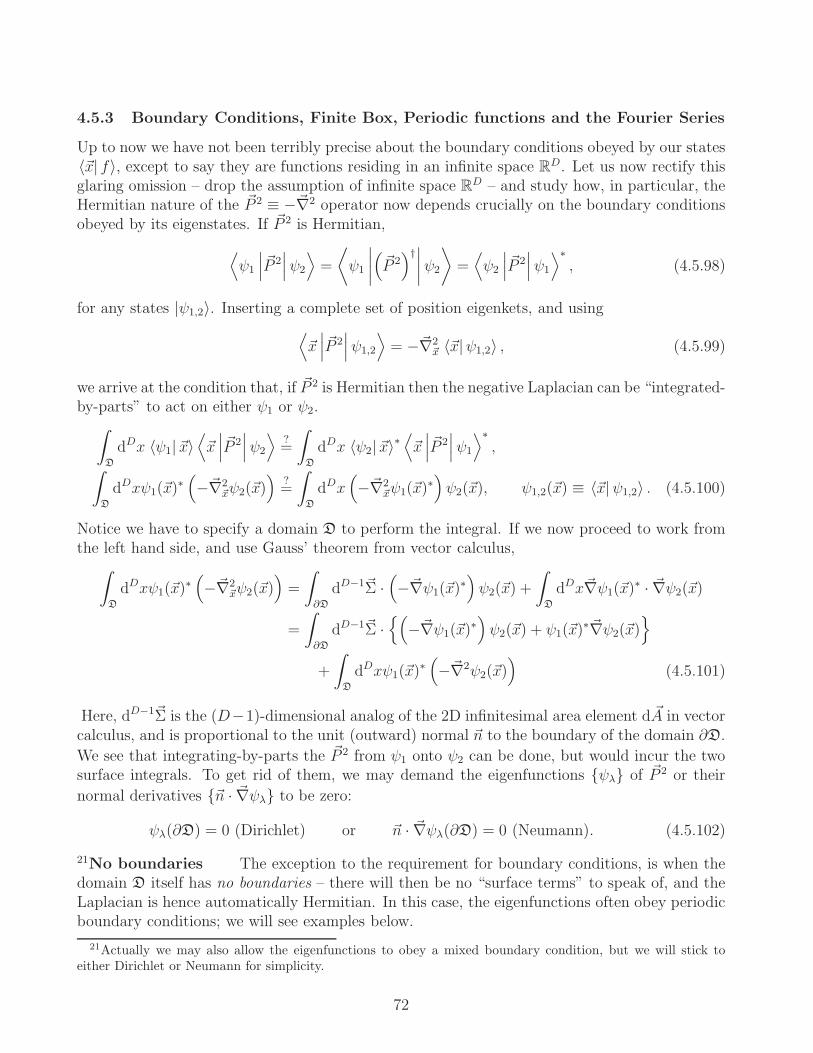
4.5.3 Boundary Conditions, Finite Box, Periodic functions and the Fourier Series

Up to now we have not been terribly precise about the boundary conditions obeyed by our states〈~x| f〉, except to say they are functions residing in an infinite space RD. Let us now rectify thisglaring omission – drop the assumption of infinite space RD – and study how, in particular, theHermitian nature of the ~P 2 ≡ −~∇2 operator now depends crucially on the boundary conditionsobeyed by its eigenstates. If ~P 2 is Hermitian,

⟨ψ1

∣∣∣ ~P 2∣∣∣ψ2

⟩=

⟨ψ1

∣∣∣∣(~P 2)†∣∣∣∣ψ2

⟩=⟨ψ2

∣∣∣~P 2∣∣∣ψ1

⟩∗, (4.5.98)

for any states |ψ1,2〉. Inserting a complete set of position eigenkets, and using

⟨~x∣∣∣~P 2∣∣∣ψ1,2

⟩= −~∇2

~x 〈~x|ψ1,2〉 , (4.5.99)

we arrive at the condition that, if ~P 2 is Hermitian then the negative Laplacian can be “integrated-by-parts” to act on either ψ1 or ψ2.∫

D

dDx 〈ψ1| ~x〉⟨~x∣∣∣ ~P 2∣∣∣ψ2

⟩?=

∫

D

dDx 〈ψ2| ~x〉∗⟨~x∣∣∣~P 2∣∣∣ψ1

⟩∗,

∫

D

dDxψ1(~x)∗(−~∇2

~xψ2(~x))

?=

∫

D

dDx(−~∇2

~xψ1(~x)∗)ψ2(~x), ψ1,2(~x) ≡ 〈~x|ψ1,2〉 . (4.5.100)

Notice we have to specify a domain D to perform the integral. If we now proceed to work fromthe left hand side, and use Gauss’ theorem from vector calculus,∫

D

dDxψ1(~x)∗(−~∇2

~xψ2(~x))=

∫

∂D

dD−1~Σ ·(−~∇ψ1(~x)

∗)ψ2(~x) +

∫

D

dDx~∇ψ1(~x)∗ · ~∇ψ2(~x)

=

∫

∂D

dD−1~Σ ·(

−~∇ψ1(~x)∗)ψ2(~x) + ψ1(~x)

∗~∇ψ2(~x)

+

∫

D

dDxψ1(~x)∗(−~∇2ψ2(~x)

)(4.5.101)

Here, dD−1~Σ is the (D−1)-dimensional analog of the 2D infinitesimal area element d ~A in vectorcalculus, and is proportional to the unit (outward) normal ~n to the boundary of the domain ∂D.

We see that integrating-by-parts the ~P 2 from ψ1 onto ψ2 can be done, but would incur the twosurface integrals. To get rid of them, we may demand the eigenfunctions ψλ of ~P 2 or their

normal derivatives ~n · ~∇ψλ to be zero:

ψλ(∂D) = 0 (Dirichlet) or ~n · ~∇ψλ(∂D) = 0 (Neumann). (4.5.102)

21No boundaries The exception to the requirement for boundary conditions, is when thedomain D itself has no boundaries – there will then be no “surface terms” to speak of, and theLaplacian is hence automatically Hermitian. In this case, the eigenfunctions often obey periodicboundary conditions; we will see examples below.

21Actually we may also allow the eigenfunctions to obey a mixed boundary condition, but we will stick toeither Dirichlet or Neumann for simplicity.

72

Summary The abstract bra-ket notation 〈ψ1|~P 2|ψ2〉 obscures the fact that boundary con-

ditions are required to ensure the Hermitian nature of ~P 2. By going to the position basis, wesee not only do we have to specify what the domain D of the underlying space is, we have toeither demand the eigenfunctions or their normal derivatives vanish on the boundary ∂D. Inthe discussion of partial differential equations below, we will generalize this analysis to curvedspaces.

Example: Finite box The first illustrative example is as follows. Suppose our systemis defined only in a finite box. For the ith Cartesian axis, the box is of length Li. If we demandthat the eigenfunctions of −~∇2 vanish at the boundary of the box, we find the eigensystem

−~∇2~x 〈~x|~n〉 = λ(~n) 〈~x|~n〉 ,

⟨~x; xi = 0

∣∣~n⟩=⟨~x; xi = Li

∣∣~n⟩= 0, (4.5.103)

i = 1, 2, 3, . . . , D, (4.5.104)

admits the solution

〈~x|~n〉 ∝D∏

i=1

sin

(πni

Lixi), λ(~n) =

D∑

i=1

(πni

Li

)2

. (4.5.105)

These ni runs over the positive integers only; because sine is an odd function, the negativeintegers do not yield new solutions.

Remark Notice that, even though ~P 2 is Hermitian in this finite box, the translation

operator T (ξ) ≡ e−i~ξ·~P is no longer unitary and the momentum operator Pj no longer Hermitian,because T (ξ) may move |x〉 out of the box if the translation distance is larger than L, and thuscan no longer be viewed as a change of basis. (Recall the discussion around eq. (4.5.50).) More

explicitly, the eigenvectors of ~P in eq. (4.5.78) do not vanish on the walls of the box – for e.g., in1D, exp(ikx) → 1 when x = 0 and exp(ikx) → exp(ikL) 6= 0 when x = L – and therefore do not

even lie in the vector space spanned by the eigenfunctions of ~P 2. (Of course, you can superposethe momentum eigenstates of different eigenvalues to obtain the states in eq. (4.5.105), but theywill no longer be eigenstates of Pj.) Furthermore, if we had instead demanded the vanishing ofthe normal derivative, ∂x exp(ikx) = ik exp(ikx) → ik 6= 0 either, unless k = 0.

Problem 4.33. Verify that the basis eigenkets in eq. (4.5.105) do solve eq. (4.5.103). Whatis the correct normalization for 〈~x|~n〉? Also verify that the basis plane waves in eq. (4.5.111)satisfy the normalization condition in eq. (4.5.110).

Periodic B.C.’s: the Fourier Series. If we stayed within the infinite space, but nowimposed periodic boundary conditions,

⟨~x; xi → xi + Li

∣∣ f⟩=⟨~x; xi

∣∣ f⟩, (4.5.106)

f(x1, . . . , xi + Li, . . . , xD) = f(x1, . . . , xi, . . . , xD) = f(~x), (4.5.107)

this would mean, not all the basis plane waves from eq. (4.5.78) remains in the Hilbert space.Instead, periodicity means

〈~x; xj = xj + Lj |~k〉 = 〈~x; xj = xj |~k〉eikj(x

j+Lj) = eikjxj

, (No sum over j.) (4.5.108)

73

(The rest of the plane waves, eiklxlfor l 6= j, cancel out of the equation.) This further implies

the eigenvalue kj becomes discrete:

eikjLj

= 1 (No sum over j.) ⇒ kjLj = 2πn ⇒ kj =

2πnj

Lj,

nj = 0,±1,±2,±3, . . . . (4.5.109)

We need to re-normalize our basis plane waves. In particular, since space is now periodic, weought to only need to integrate over one typical volume.

∫

0≤xi≤Li|i=1,2,...,D

dD~x 〈~n′|~x〉 〈~x|~n〉 = δ~n~n′ ≡D∏

i=1

δn′i

ni . (4.5.110)

Because we have a set of orthonormal eigenvectors of the negative Laplacian,

〈~x |~n〉 ≡D∏

j=1

exp(i2πn

j

Lj xj)

√Lj

, (4.5.111)

−~∇2 〈~x |~n〉 = λ(~n) 〈~x |~n〉 , λ(~n) =∑

i

(2πni

Li

)2

; (4.5.112)

they obey the completeness relation

〈~x| ~x′〉 = δ(D)(~x− ~x′) =∞∑

n1=−∞

· · ·∞∑

nD=−∞

〈~x|~n〉 〈~n| ~x′〉 . (4.5.113)

To sum: any periodic function f , subject to eq. (4.5.107), can be expanded as a superpositionof periodic plane waves in eq. (4.5.111),

f(~x) =

∞∑

n1=−∞

· · ·∞∑

nD=−∞

f(n1, . . . , nD)

D∏

j=1

(Lj)−1/2 exp

(i2πnj

Ljxj). (4.5.114)

This is known as the Fourier series. By using the inner product in eq. (4.5.110), or equivalently,multiplying both sides of eq. (4.5.114) by

∏j(L

j)−1/2 exp(−i(2πn′j/Lj)xj) and integrating overa typical volume, we obtain the coefficients of the Fourier series expansion

f(n1, n2, . . . , nD) =

∫

0≤xj≤Lj

dD~xf(~x)

D∏

j=1

(Lj)−1/2 exp

(−i2πn

j

Ljxj). (4.5.115)

Remark I The exp in eq. (4.5.111) are not a unique set of basis vectors, of course. Onecould use sines and cosines instead, for example.Remark II Even though we are explicitly integrating the ith Cartesian coordinate from 0to Li in eq. (4.5.115), since the function is periodic, we really just need only to integrate over acomplete period, from κ to κ + Li (for κ real), to achieve the same result. For example, in 1D,and whenever f(x) is periodic (with a period of L),

∫ L

0

dxf(x) =

∫ κ+L

κ

dxf(x). (4.5.116)

(Drawing a plot here may help to understand this statement.)

74

5 Calculus on the Complex Plane

5.1 Differentiation22The derivative of a complex function f(z) is defined in a similar way as its real counterpart:

f ′(z) ≡ df(z)

dz≡ lim

∆z→0

f(z +∆z)− f(z)

∆z. (5.1.1)

However, the meaning is more subtle because ∆z (just like z itself) is now complex. What thismeans is that, in taking this limit, it has to yield the same answer no matter what direction youapproach z on the complex plane. For example, if z = x + iy, taking the derivative along thereal direction must be equal to that along the imaginary one,

f ′(z) = lim∆x→0

f(x+∆x+ iy)− f(x+ iy)

∆x= ∂xf(z)

= lim∆y→0

f(x+ i(y +∆y))− f(x+ iy)

i∆y=∂f(z)

∂(iy)=

1

i∂yf(z), (5.1.2)

where x, y, ∆x and ∆y are real. This direction independence imposes very strong constraints oncomplex differentiable functions: they will turn out to be extremely smooth, in that if you candifferentiate them at a given point z, you are guaranteed they are differentiable infinite numberof times there. (This is not true of real functions.) If f(z) is differentiable in some region on thecomplex plane, we say f(z) is analytic there.

If the first derivatives of f(z) are continuous, the criteria for determining whether f(z) isdifferentiable comes in the following pair of partial differential equations.

Cauchy-Riemann conditions for analyticity Let z = x+ iy and f(z) =u(x, y) + iv(x, y), where x, y, u and v are real. Let u and v have continuous firstpartial derivatives in x and y. Then f(z) is an analytic function in the neighborhoodof z if and only if the following (Cauchy-Riemann) equations are satisfied by the realand imaginary parts of f :

∂xu = ∂yv, ∂yu = −∂xv. (5.1.3)

To understand why this is true, we first consider differentiating along the (real) x direction, we’dhave

df(z)

dz= ∂xu+ i∂xv. (5.1.4)

If we differentiate along the (imaginary) iy direction instead, we’d have

df(z)

dz=

1

i∂yu+ ∂yv = ∂yv − i∂yu. (5.1.5)

Since these two results must be the same, we may equate their real and imaginary parts to obtaineq. (5.1.3). (It is at this point, if we did not assume u and v have continuous first derivatives,

22Much of the material here on complex analysis is based on Arfken et al’sMathematical Methods for Physicists.

75

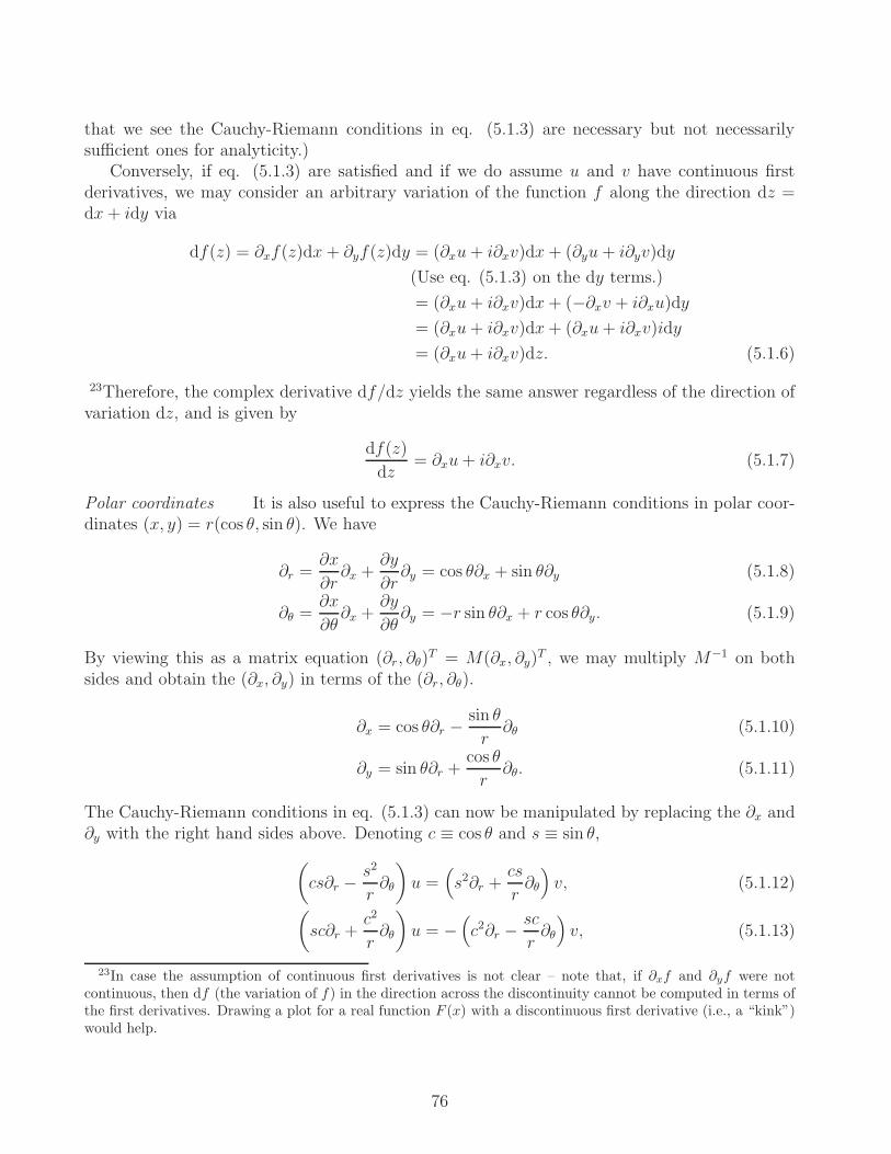
that we see the Cauchy-Riemann conditions in eq. (5.1.3) are necessary but not necessarilysufficient ones for analyticity.)

Conversely, if eq. (5.1.3) are satisfied and if we do assume u and v have continuous firstderivatives, we may consider an arbitrary variation of the function f along the direction dz =dx+ idy via

df(z) = ∂xf(z)dx+ ∂yf(z)dy = (∂xu+ i∂xv)dx+ (∂yu+ i∂yv)dy

(Use eq. (5.1.3) on the dy terms.)

= (∂xu+ i∂xv)dx+ (−∂xv + i∂xu)dy

= (∂xu+ i∂xv)dx+ (∂xu+ i∂xv)idy

= (∂xu+ i∂xv)dz. (5.1.6)

23Therefore, the complex derivative df/dz yields the same answer regardless of the direction ofvariation dz, and is given by

df(z)

dz= ∂xu+ i∂xv. (5.1.7)

Polar coordinates It is also useful to express the Cauchy-Riemann conditions in polar coor-dinates (x, y) = r(cos θ, sin θ). We have

∂r =∂x

∂r∂x +

∂y

∂r∂y = cos θ∂x + sin θ∂y (5.1.8)

∂θ =∂x

∂θ∂x +

∂y

∂θ∂y = −r sin θ∂x + r cos θ∂y. (5.1.9)

By viewing this as a matrix equation (∂r, ∂θ)T = M(∂x, ∂y)

T , we may multiply M−1 on bothsides and obtain the (∂x, ∂y) in terms of the (∂r, ∂θ).

∂x = cos θ∂r −sin θ

r∂θ (5.1.10)

∂y = sin θ∂r +cos θ

r∂θ. (5.1.11)

The Cauchy-Riemann conditions in eq. (5.1.3) can now be manipulated by replacing the ∂x and∂y with the right hand sides above. Denoting c ≡ cos θ and s ≡ sin θ,

(cs∂r −

s2

r∂θ

)u =

(s2∂r +

cs

r∂θ

)v, (5.1.12)

(sc∂r +

c2

r∂θ

)u = −

(c2∂r −

sc

r∂θ

)v, (5.1.13)

23In case the assumption of continuous first derivatives is not clear – note that, if ∂xf and ∂yf were notcontinuous, then df (the variation of f) in the direction across the discontinuity cannot be computed in terms ofthe first derivatives. Drawing a plot for a real function F (x) with a discontinuous first derivative (i.e., a “kink”)would help.

76

and(c2∂r −

sc

r∂θ

)u =

(sc∂r +

c2

r∂θ

)v, (5.1.14)

(s2∂r +

sc

r∂θ

)u = −

(cs∂r −

s2

r∂θ

)v. (5.1.15)

(We have multiplied both sides of eq. (5.1.3) with appropriate factors of sines and cosines.) Sub-tracting the first pair and adding the second pair of equations, we arrive at the polar coordinatesversion of Cauchy-Riemann:

1

r∂θu = −∂rv, ∂ru =

1

r∂θv. (5.1.16)

Examples Complex differentiability is much more restrictive than the real case. An exampleis f(z) = |z|. If z is real, then at least for z 6= 0, we may differentiate f(z) – the result isf ′(z) = 1 for z > 0 and f ′(z) = −1 for z < 0. But in the complex case we would identify, withz = x+ iy,

f(z) = |z| =√x2 + y2 = u(x, y) + iv(x, y) ⇒ v(x, y) = 0. (5.1.17)

It’s not hard to see that the Cauchy-Riemann conditions in eq. (5.1.3) cannot be satisfied sincev is zero while u is non-zero. In fact, any f(z) that remains strictly real across the complex zplane is not differentiable unless f(z) is constant.

f(z) = u(x, y) ⇒ ∂xu = ∂yv = 0, ∂yu = −∂xv = 0. (5.1.18)

Similarly, if f(z) were purely imaginary across the complex z plane, it is not differentiable unlessf(z) is constant.

f(z) = iv(x, y) ⇒ 0 = ∂xu = ∂yv, 0 = −∂yu = ∂xv. (5.1.19)

Differentiation rules If you know how to differentiate a function f(z) when z is real,then as long as you can show that f ′(z) exists, the differentiation formula for the complex casewould carry over from the real case. That is, suppose f ′(z) = g(z) when f , g and z are real;then this form has to hold for complex z. For example, powers are differentiated the same way

d

dzzα = αzα−1, α ∈ R, (5.1.20)

and

d sin(z)

dz= cos z,

daz

dz=

dez lna

dz= az ln a. (5.1.21)

It is not difficult to check the first derivatives of zα, sin(z) and az are continuous; and theCauchy-Riemann conditions are satisfied. For instance, zα = rαeiαθ = rα cos(αθ) + irα sin(αθ)and eq. (5.1.16) can be verified.

rα−1∂θ cos(αθ) = −αrα−1 sin(αθ)?= − sin(αθ)∂rr

α = −αrα−1 sin(αθ), (5.1.22)

cos(αθ)∂rrα = αrα−1 cos(αθ)

?= rα−1∂θ sin(αθ) = αrα−1 cos(αθ). (5.1.23)

77

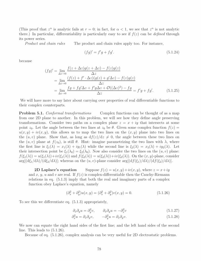
(This proof that zα is analytic fails at r = 0; in fact, for α < 1, we see that zα is not analyticthere.) In particular, differentiability is particularly easy to see if f(z) can be defined throughits power series.

Product and chain rules The product and chain rules apply too. For instance,

(fg)′ = f ′g + fg′. (5.1.24)

because

(fg)′ = lim∆z→0

f(z +∆z)g(z +∆z)− f(z)g(z)

∆z

= lim∆z→0

(f(z) + f ′ ·∆z)(g(z) + g′∆z)− f(z)g(z)

∆z

= lim∆z→0

fg + fg′∆z + f ′g∆z +O((∆z)2)− fg

∆z= f ′g + fg′. (5.1.25)

We will have more to say later about carrying over properties of real differentiable functions totheir complex counterparts.

Problem 5.1. Conformal transformations Complex functions can be thought of as a mapfrom one 2D plane to another. In this problem, we will see how they define angle preservingtransformations. Consider two paths on a complex plane z = x + iy that intersects at somepoint z0. Let the angle between the two lines at z0 be θ. Given some complex function f(z) =u(x, y) + iv(x, y), this allows us to map the two lines on the (x, y) plane into two lines onthe (u, v) plane. Show that, as long as df(z)/dz 6= 0, the angle between these two lines onthe (u, v) plane at f(z0), is still θ. Hint: imagine parametrizing the two lines with λ, wherethe first line is ξ1(λ) = x1(λ) + iy1(λ) while the second line is ξ2(λ) = x2(λ) + iy2(λ). Lettheir intersection point be ξ1(λ0) = ξ2(λ0). Now also consider the two lines on the (u, v) plane:f(ξ1(λ)) = u(ξ1(λ))+iv(ξ1(λ)) and f(ξ2(λ)) = u(ξ2(λ))+iv(ξ2(λ)). On the (x, y)-plane, considerarg[(dξ1/dλ)/(dξ2/dλ)]; whereas on the (u, v)-plane consider arg[(df(ξ1)/dλ)/(df(ξ2)/dλ)].

2D Laplace’s equation Suppose f(z) = u(x, y)+ iv(x, y), where z = x+ iyand x, y, u and v are real. If f(z) is complex-differentiable then the Cauchy-Riemannrelations in eq. (5.1.3) imply that both the real and imaginary parts of a complexfunction obey Laplace’s equation, namely

(∂2x + ∂2y)u(x, y) = (∂2x + ∂2y)v(x, y) = 0. (5.1.26)

To see this we differentiate eq. (5.1.3) appropriately,

∂x∂yu = ∂2yv, ∂x∂yu = −∂2xv (5.1.27)

∂2xu = ∂x∂yv, −∂2yu = ∂x∂yv. (5.1.28)

We now can equate the right hand sides of the first line; and the left hand sides of the secondline. This leads to (5.1.26).

Because of eq. (5.1.26), complex analysis can be very useful for 2D electrostatic problems.

78

Moreover, u and v cannot admit local minimum or maximums, as long as ∂2xu and ∂2xv arenon-zero. In particular, the determinants of the 2× 2 Hessian matrices ∂2u/∂(x, y)i∂(x, y)j and∂2v/∂(x, y)i∂(x, y)j – and hence the product of their eigenvalues – are negative. For,

det∂2u

∂(x, y)i∂(x, y)j= det

[∂2xu ∂x∂yu∂x∂yu ∂2yu

]

= ∂2xu∂2yu− (∂x∂yu)

2 = −(∂2yu)2 − (∂2yv)

2 ≤ 0, (5.1.29)

det∂2v

∂(x, y)i∂(x, y)j= det

[∂2xv ∂x∂yv∂x∂yv ∂2yv

]

= ∂2xv∂2yv − (∂x∂yv)

2 = −(∂2yv)2 − (∂2yu)

2 ≤ 0, (5.1.30)

where both equations (5.1.26) and (5.1.27) were employed.

5.2 Cauchy’s integral theorems, Laurent Series, Analytic Continua-tion

Complex integration is really a line integral∫~ξ · (dx, dy) on the 2D complex plane. Given some

path (aka “contour”) C, defined by z(λ1 ≤ λ ≤ λ2) = x(λ) + iy(λ), with z(λ1) = z1 andz(λ2) = z2,

∫

C

dzf(z) =

∫

z(λ1≤λ≤λ2)

(dx+ idy) (u(x, y) + iv(x, y))

=

∫

z(λ1≤λ≤λ2)

(udx− vdy) + i

∫

z(λ1≤λ≤λ2)

(vdx+ udy)

=

∫ λ2

λ1

dλ

(udx(λ)

dλ− v

dy(λ)

dλ

)+ i

∫ λ2

λ1

dλ

(vdx(λ)

dλ+ u

dy(λ)

dλ

). (5.2.1)

The real part of the line integral involves Re~ξ = (u,−v) and its imaginary part Im~ξ = (v, u).Remark I Because complex integration is a line integral, reversing the direction of contourC (which we denote as −C) would yield return negative of the original integral.

∫

−C

dzf(z) = −∫

C

dzf(z) (5.2.2)

Remark II The complex version of the fundamental theorem of calculus has to hold, in that∫

C

dzf ′(z) =

∫

C

df = f(“upper” end point of C)− f(“lower” end point of C)

=

∫ z2

z1

dzf ′(z) = f(z2)− f(z1). (5.2.3)

Cauchy’s integral theorem In introducing the contour integral in eq.(5.2.1), we are not assuming any properties about the integrand f(z). However,if the complex function f(z) is analytic throughout some simply connected region24

24A simply connected region is one where every closed loop in it can be shrunk to a point.

79

containing the contour C, then we are lead to one of the key results of complexintegration theory: the integral of f(z) within any closed path C there is zero.

∮

C

f(z)dz = 0 (5.2.4)

Unfortunately the detailed proof will take up too much time and effort, but the mathematicallyminded can consult, for example, Brown and Churchill’s Complex Variables and Applications.

Problem 5.2. If the first derivatives of f(z) are assumed to be continuous, then a proofof this modified Cauchy’s theorem can be carried out by starting with the view that

∮Cf(z)dz

is a (complex) line integral around a closed loop. Then apply Stokes’ theorem followed by theCauchy-Riemann conditions in eq. (5.1.3). Can you fill in the details?

Important Remarks Cauchy’s theorem has an important implication. Suppose we have acontour integral

∫Cg(z)dz, where C is some arbitrary (not necessarily closed) contour. Suppose

we have another contour C ′ whose end points coincide with those of C. If the function g(z) isanalytic inside the region bounded by C and C ′, then it has to be that

∫

C

g(z)dz =

∫

C′g(z)dz. (5.2.5)

The reason is that, by subtracting these two integrals, say (∫C−∫C′)g(z)dz, the − sign can be

absorbed by reversing the direction of the C ′ integral. We then have a closed contour integral(∫C−∫C′)g(z)dz =

∮g(z)dz and Cauchy’s theorem in eq. (5.2.4) applies.

This is a very useful observation because it means, for a given contour integral, you candeform the contour itself to a shape that would make the integral easier to evaluate. Below, wewill generalize this and show that, even if there are isolated points where the function is notanalytic, you can still pass the contour over these points, but at the cost of incurring additionalterms resulting from taking the residues there. Another possible type of singularity is known asa branch point, which will then require us to introduce a branch cut.

Note that the simply connected requirement can often be circumvented by considering anappropriate cut line. For example, suppose C1 and C2 were both counterclockwise (or bothclockwise) contours around an annulus region, within which f(z) is analytic. Then

∮

C1

f(z)dz =

∮

C2

f(z)dz. (5.2.6)

Example I A simple but important example is the following integral, where the contour Cis an arbitrary counterclockwise closed loop that encloses the point z = 0.

I ≡∮

C

dz

z(5.2.7)

Cauchy’s integral theorem does not apply directly because 1/z is not analytic at z = 0. Byconsidering a counterclockwise circle C ′ of radius R > 0, however, we may argue

∮

C

dz

z=

∮

C′

dz

z. (5.2.8)

80

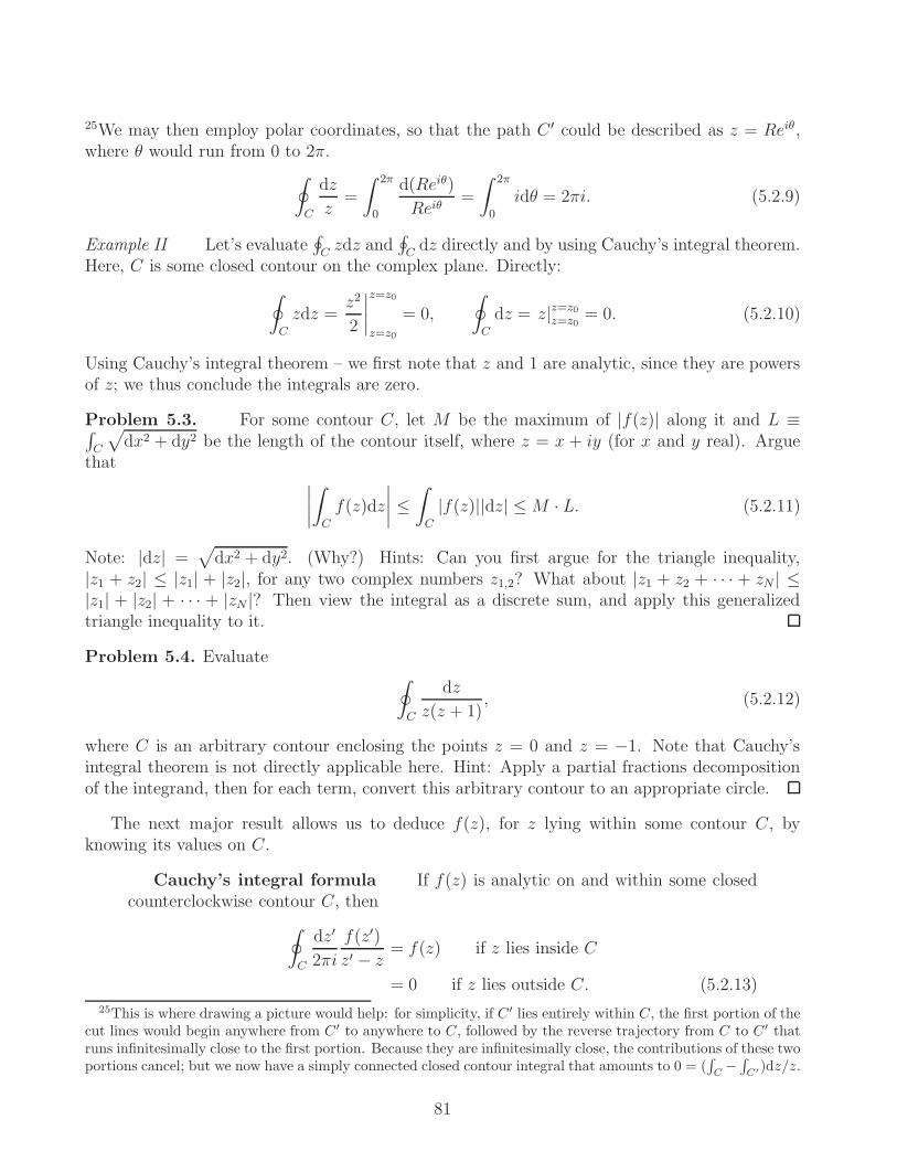
25We may then employ polar coordinates, so that the path C ′ could be described as z = Reiθ,where θ would run from 0 to 2π.

∮

C

dz

z=

∫ 2π

0

d(Reiθ)

Reiθ=

∫ 2π

0

idθ = 2πi. (5.2.9)

Example II Let’s evaluate∮Czdz and

∮Cdz directly and by using Cauchy’s integral theorem.

Here, C is some closed contour on the complex plane. Directly:

∮

C

zdz =z2

2

∣∣∣∣z=z0

z=z0

= 0,

∮

C

dz = z|z=z0z=z0

= 0. (5.2.10)

Using Cauchy’s integral theorem – we first note that z and 1 are analytic, since they are powersof z; we thus conclude the integrals are zero.

Problem 5.3. For some contour C, let M be the maximum of |f(z)| along it and L ≡∫C

√dx2 + dy2 be the length of the contour itself, where z = x + iy (for x and y real). Argue

that∣∣∣∣∫

C

f(z)dz

∣∣∣∣ ≤∫

C

|f(z)||dz| ≤M · L. (5.2.11)

Note: |dz| =√

dx2 + dy2. (Why?) Hints: Can you first argue for the triangle inequality,|z1 + z2| ≤ |z1| + |z2|, for any two complex numbers z1,2? What about |z1 + z2 + · · · + zN | ≤|z1| + |z2| + · · · + |zN |? Then view the integral as a discrete sum, and apply this generalizedtriangle inequality to it.

Problem 5.4. Evaluate∮

C

dz

z(z + 1), (5.2.12)

where C is an arbitrary contour enclosing the points z = 0 and z = −1. Note that Cauchy’sintegral theorem is not directly applicable here. Hint: Apply a partial fractions decompositionof the integrand, then for each term, convert this arbitrary contour to an appropriate circle.

The next major result allows us to deduce f(z), for z lying within some contour C, byknowing its values on C.

Cauchy’s integral formula If f(z) is analytic on and within some closedcounterclockwise contour C, then

∮

C

dz′

2πi

f(z′)

z′ − z= f(z) if z lies inside C

= 0 if z lies outside C. (5.2.13)

25This is where drawing a picture would help: for simplicity, if C′ lies entirely within C, the first portion of thecut lines would begin anywhere from C′ to anywhere to C, followed by the reverse trajectory from C to C′ thatruns infinitesimally close to the first portion. Because they are infinitesimally close, the contributions of these twoportions cancel; but we now have a simply connected closed contour integral that amounts to 0 = (

∫C−∫C′)dz/z.

81

Proof If z lies outside C then the integrand is analytic within its interior and thereforeCauchy’s integral theorem applies. If z lies within C we may then deform the contour such thatit becomes an infinitesimal counterclockwise circle around z′ ≈ z,

z′ ≡ z + ǫeiθ, 0 < ǫ≪ 1. (5.2.14)

We then have

∮

C

dz′

2πi

f(z′)

z′ − z=

1

2πi

∫ 2π

0

ǫeiθidθf(z + ǫeiθ)

ǫeiθ

=

∫ 2π

0

dθ

2πf(z + ǫeiθ). (5.2.15)

By taking the limit ǫ→ 0+, we get f(z), since f(z′) is analytic and thus continuous at z′ = z.

Cauchy’s integral formula for derivatives By applying the limit defini-tion of the derivative, we may obtain an analogous definition for the nth derivativeof f(z). For some closed counterclockwise contour C,

∮

C

dz′

2πi

f(z′)

(z′ − z)n+1=f (n)(z)

n!if z lies inside C

= 0 if z lies outside C. (5.2.16)

This implies – as already advertised earlier – once f ′(z) exists, f (n)(z) also exists for any n.Complex-differentiable functions are infinitely smooth.

The converse of Cauchy’s integral formula is known as Morera’s theorem, which we willsimply state without proof.

Morera’s theorem If f(z) is continuous in a simply connected region and∮Cf(z)dz = 0 for any closed contour C within it, then f(z) is analytic throughout

this region.

Now, even though f (n>1)(z) exists once f ′(z) exists (cf. (5.2.16)), f(z) cannot be infinitelysmooth everywhere on the complex z−plane..

Liouville’s theorem If f(z) is analytic and bounded – i.e., |f(z)| is less thansome positive constant M – for all complex z, then f(z) must in fact be a constant.Apart from the constant function, analytic functions must blow up somewhere onthe complex plane.

Proof To prove this result we employ eq. (5.2.16). Choose a counterclockwise circularcontour C that encloses some arbitrary point z,

|f (n)(z)| ≤ n!

∮

C

|dz′|2π

|f(z′)||(z′ − z)n+1| (5.2.17)

≤ n!M

2πrn+1

∮

C

|dz′| = n!M

rn. (5.2.18)

82

Here, r is the radius from z to C. But by Cauchy’s theorem, the circle can be made arbitrarilylarge. By sending r → ∞, we see that |f (n)(z)| = 0, the nth derivative of the analytic functionat an arbitrary point z is zero for any integer n ≥ 1. This proves the theorem.

Examples The exponential ez while differentiable everywhere on the complex plane,does in fact blow up at Re z → ∞. Sines and cosines are oscillatory and bounded on the realline; and are differentiable everywhere on the complex plane. However, they blow up as onemove towards positive or negative imaginary infinity. Remember sin(z) = (eiz − e−iz)/(2i) andcos(z) = (eiz + e−iz)/2. Then, for R ∈ R,

sin(iR) =e−R − eR

2i, cos(iR) =

e−R + eR

2. (5.2.19)

Both sin(iR) and cos(iR) blow up as R → ±∞.

Problem 5.5. Fundamental theorem of algebra. Let P (z) = p0 + p1z + . . . pnzn be an nth

degree polynomial, where n is an integer greater or equal to 1. By considering f(z) = 1/P (z),show that P (z) has at least one root. (Once a root has been found, we can divide it out fromP (z) and repeat the argument for the remaining (n− 1)-degree polynomial. By induction, thisimplies an nth degree polynomial has exactly n roots – this is the fundamental theorem ofalgebra.)

Taylor series The generalization of the Taylor series of a real differentiable function tothe complex case is known as the Laurent series. If the function is completely smooth in someregion on the complex plane, then we shall see that it can in fact be Taylor expanded the usualway, except the expressions are now complex. If there are isolated points where the functionblows up, then it can be (Laurent) expanded about those points, in powers of the complexvariable – except the series begins at some negative integer power, as opposed to the zerothpower in the usual Taylor series.

To begin, let us show that the geometric series still works in the complex case.

Problem 5.6. By starting with the Nth partial sum,

SN ≡N∑

ℓ=0

tℓ, (5.2.20)

prove that, as long as |t| < 1,

1

1− t=

∞∑

ℓ=0

tℓ. (5.2.21)

Now pick a point z0 on the complex plane and identify the nearest point, say z1, where fis no longer analytic. Consider some closed counterclockwise contour C that lies within thecircular region |z − z0| < |z1 − z0|. Then we may apply Cauchy’s integral formula eq. (5.2.13),

83

and deduce a series expansion about z0:

f(z) =

∮

C

dz′

2πi

f(z′)

z′ − z

=

∮

C

dz′

2πi

f(z′)

(z′ − z0)− (z − z0)=

∮

C

dz′

2πi

f(z′)

(z′ − z0)(1− (z − z0)/(z′ − z0))

=

∞∑

ℓ=0

∮

C

dz′

2πi

f(z′)

(z′ − z0)ℓ+1(z − z0)

ℓ . (5.2.22)

We have used the geometric series in eq. (5.2.21) and the fact that it converges uniformly tointerchange the order of integration and summation. At this point, if we now recall Cauchy’sintegral formula for the nth derivative of an analytic function, eq. (5.2.16), we have arrived atits Taylor series.

Taylor series For f(z) complex analytic within the circular region |z− z0| <|z1 − z0|, where z1 is the nearest point to z0 where f is no longer differentiable,

f(z) =

∞∑

ℓ=0

(z − z0)ℓf

(ℓ)(z0)

ℓ!, (5.2.23)

where f (ℓ)(z)/ℓ! is given by eq. (5.2.16).

Problem 5.7. Complex binomial theorem. For p any real number and z any complexnumber obeying |z| < 1, prove the complex binomial theorem using eq. (5.2.23),

(1 + z)p =∞∑

ℓ=0

(p

ℓ

)zℓ,

(p

0

)≡ 1,

(p

ℓ

)=p(p− 1) . . . (p− (ℓ− 1))

ℓ!. (5.2.24)

Laurent series We are now ready to derive the Laurent expansion of a function f(z) thatis analytic within an annulus, say bounded by the circles |z − z0| = r1 and |z − z0| = r2 > r1.That is, the center of the annulus region is z0 and the smaller circle has radius r1 and larger oner2. To start, we let C1 be a clockwise circular contour with radius r2 > r′1 > r1 and let C2 be acounterclockwise circular contour with radius r2 > r′2 > r′1 > r1. As long as z lies between thesetwo circular contours, we have

f(z) =

(∫

C1

+

∫

C2

)dz′

2πi

f(z′)

z′ − z. (5.2.25)

Strictly speaking, we need to integrate along a cut line joining the C1 and C2 – and another oneinfinitesimally close to it, in the opposite direction – so that we can form a closed contour. Butby assumption f(z) is analytic and therefore continuous; the integrals along these pair of cutlines must cancel. For the C1 integral, we may write z′ − z = −(z − z0)(1 − (z′ − z0)/(z − z0))and apply the geometric series in eq. (5.2.21) because |(z′ − z0)/(z− z0)| < 1. Similarly, for theC2 integral, we may write z′ − z = (z′ − z0)(1− (z − z0)/(z

′ − z0)) and geometric series expandthe right factor because |(z − z0)/(z

′ − z0)| < 1. These lead us to

f(z) =

∞∑

ℓ=0

(z − z0)ℓ

∫

C2

dz′

2πi

f(z′)

(z′ − z0)ℓ+1−

∞∑

ℓ=0

1

(z − z0)ℓ+1

∫

C1

dz′

2πi(z′ − z0)

ℓf(z′). (5.2.26)

84

Remember complex integration can be thought of as a line integral, which reverses sign if wereverse the direction of the line integration. Therefore we may absorb the − sign in front ofthe C1 integral(s) by turning C1 from a clockwise circle into C ′

1 = −C1, a counterclockwise one.Moreover, note that we may now deform the contour C ′

1 into C2,

∫

C′1

dz′

2πi(z′ − z0)

ℓf(z′) =

∫

C2

dz′

2πi(z′ − z0)

ℓf(z′), (5.2.27)

because for positive ℓ the integrand (z′ − z0)ℓf(z′) is analytic in the region lying between the

circles C ′1 and C2. At this point we have

f(z) =

∞∑

ℓ=0

∫

C2

dz′

2πi

((z − z0)

ℓ f(z′)

(z′ − z0)ℓ+1+

1

(z − z0)ℓ+1(z′ − z0)

ℓf(z′)

). (5.2.28)

Proceeding to re-label the second series by replacing ℓ + 1 → −ℓ′, so that the summation thenruns from −1 through −∞, the Laurent series emerges.

Laurent series Let f(z) be analytic within the annulus r1 < |z − z0| < r2 <|z1−z0|, where z0 is some complex number such that f(z) may not be analytic within|z − z0| < r1; z1 is the nearest point outside of |z − z0| ≥ r1 where f(z) fails to bedifferentiable; and the radii r2 > r1 > 0 are real positive numbers. The Laurentexpansion of f(z) about z0, valid throughout the entire annulus, reads

f(z) =

∞∑

ℓ=−∞

Lℓ(z0) · (z − z0)ℓ, (5.2.29)

Lℓ(z0) ≡∫

C

dz′

2πi

f(z′)

(z′ − z0)ℓ+1. (5.2.30)

The C is any counterclockwise closed contour containing both z and the inner circle|z − z0| = r1.

Uniqueness It is worth asserting that the Laurent expansion of a function, in the regionwhere it is analytic, is unique. That means it is not always necessary to perform the integralsin eq. (5.2.29) to obtain the expansion coefficients Lℓ.

Problem 5.8. For complex z, a and b, obtain the Laurent expansion of

f(z) ≡ 1

(z − a)(z − b), a 6= b, (5.2.31)

about z = a, in the region 0 < |z − a| < |a− b| using eq. (5.2.29). Check your result either bywriting

1

z − b= − 1

1− (z − a)/(b− a)

1

b− a. (5.2.32)

and employing the geometric series in eq. (5.2.21), or directly performing a Taylor expansion of1/(z − b) about z = a.

85

Problem 5.9. Schwarz reflection principle. Proof the following statement using Laurentexpansion. If a function f(z = x+ iy) = u(x, y)+ iv(x, y) can be Laurent expanded (for x, y, u,and v real) about some point on the real line, and if f(z) is real whenever z is real, then

(f(z))∗ = u(x, y)− iv(x, y) = f(z∗) = u(x,−y) + iv(x,−y). (5.2.33)

Comment on why this is called the “reflection principle”.

We now turn to an important result that allows us to extend the definitions of complex differ-entiable functions beyond their original range of validity.

Analytic continuation An analytic function f(z) is fixed uniquely through-out a given region Σ on the complex plane, once its value is specified on a line segmentlying within Σ.

This in turn means, suppose we have an analytic function f1(z) defined in a region Σ1 on thecomplex plane, and suppose we found another analytic function f2(z) defined in some region Σ2

such that f2(z) agrees with f1(z) in their common region of intersection. (It is important thatΣ2 does have some overlap with Σ1.) Then we may view f2(z) as an analytic continuation off1(z), because this extension is unique – it is not possible to find a f3(z) that agrees with f1(z)in the common intersection between Σ1 and Σ2, yet behave different in the rest of Σ2.

These results inform us, any real differentiable function we are familiar with can be extendedto the complex plane, simply by knowing its Taylor expansion. For example, ex is infinitelydifferentiable on the real line, and its definition can be readily extended into the complex planevia its Taylor expansion.

An example of analytic continuation is that of the geometric series. If we define

f1(z) ≡∞∑

ℓ=0

zℓ, |z| < 1, (5.2.34)

and

f2(z) ≡1

1− z, (5.2.35)

then we know they agree in the region |z| < 1 and therefore any line segment within it. Butwhile f1(z) is defined only in this region, f2(z) is valid for any z 6= 1. Therefore, we may view1/(1− z) as the analytic continuation of f1(z) for the region |z| > 1. Also observe that we cannow understand why the series is valid only for |z| < 1: the series of f1(z) is really the Taylorexpansion of f2(z) about z = 0, and since the nearest singularity is at z = 1, the circular regionof validity employed in our (constructive) Taylor series proof is in fact |z| < 1.

Problem 5.10. One key application of analytic continuation is that, some special functionsin mathematical physics admit a power series expansion that has a finite radius of convergence.This can occur if the differential equations they solve have singular points. Many of these specialfunctions also admit an integral representation, whose range of validity lies beyond that of thepower series. This allows the domain of these special functions to be extended.

86

The hypergeometric function 2F1(α, β; γ; z) is such an example. For |z| < 1 it has a powerseries expansion

2F1(α, β; γ; z) =

∞∑

ℓ=0

Cℓ(α, β; γ)zℓ

ℓ!,

C0(α, β; γ) ≡ 1,

Cℓ≥1(α, β; γ) ≡α(α + 1) . . . (α + (ℓ− 1)) · β(β + 1) . . . (β + (ℓ− 1))

γ(γ + 1) . . . (γ + (ℓ− 1)). (5.2.36)

On the other hand, it also has the following integral representation,

2F1(α, β; γ; z) =Γ(γ)

Γ(γ − β)Γ(β)

∫ 1

0

tβ−1(1− t)γ−β−1(1− tz)−αdt, Re(γ) >Re(β) > 0.

(5.2.37)

(Here, Γ(z) is known as the Gamma function; see http://dlmf.nist.gov/5.) Show that eq. (5.2.37)does in fact agree with eq. (5.2.36) for |z| < 1. You can apply the binomial expansion in eq.(5.2.24) to (1− tz)−α, followed by result

∫ 1

0

dt(1− t)α−1tβ−1 =Γ(α)Γ(β)

Γ(α + β), Re(α), Re(β) > 0. (5.2.38)

You may also need the property

zΓ(z) = Γ(z + 1). (5.2.39)

Therefore eq. (5.2.37) extends eq. (5.2.36) into the region |z| > 1.

5.3 Poles and Residues

In this section we will consider the closed counterclockwise contour integral

∮

C

dz

2πif(z), (5.3.1)

where f(z) is analytic everywhere on and within C except at isolated singular points of f(z) –which we will denote as z1, . . . , zn, for (n ≥ 1)-integer. That is, we will assume there is noother type of singularities. We will show that the result is the sum of the residues of f(z) atthese points. This case will turn out to have a diverse range of physical applications, includingthe study of the vibrations of black holes.

We begin with some jargon.Nomenclature If a function f(z) admits a Laurent expansion about z = z0 starting

from 1/(z − z0)m, for m some positive integer,

f(z) =

∞∑

ℓ=−m

Lℓ · (z − z0)ℓ, (5.3.2)

87

we say the function has a pole of order m at z = z0. If m = ∞ we say the function has anessential singularity. The residue of a function f at some location z0 is simply the coefficientL−1 of the negative one power (ℓ = −1 term) of the Laurent series expansion about z = z0.

The key to the result already advertised is the following.

Problem 5.11. If n is an arbitrary integer, show that∮

C

(z′ − z)ndz′

2πi= 1, when n = −1,

= 0, when n 6= −1, (5.3.3)

where C is any contour (whose interior defines a simply connected domain) that encloses thepoint z′ = z.

By assumption, we may deform our contour C so that they become the collection of closedcounterclockwise contours C ′

i|i = 1, 2, . . . , n around each and every isolated point. This means∮

C

f(z′)dz′

2πi=∑

i

∮

C′i

f(z′)dz′

2πi. (5.3.4)

Strictly speaking, to preserve the full closed contour structure of the original C, we need to jointhese new contours – say C ′

i to C′i+1, C

′i+1 to C ′

i+2, and so on – by a pair of contour lines placedinfinitesimally apart, for e.g., one from C ′

i → C ′i+1 and the other C ′

i+1 → C ′i. But by assumption

f(z) is analytic and therefore continuous there, and thus the contribution from these pairs willsurely cancel. Let us perform a Laurent expansion of f(z) about zi, the ith singular point, andthen proceed to integrate the series term-by-term using eq. (5.3.3).

∮

C′i

f(z′)dz′

2πi=

∫

C′i

∞∑

ℓ=−mi

L(i)ℓ · (z′ − zi)

ℓ dz′

2πi= L

(i)−1. (5.3.5)

Residue theorem As advertised, the closed counterclockwise contour in-tegral of a function that is analytic everywhere on and within the contour, exceptat isolated points zi, yields the sum of the residues at each of these points. Inequation form,

∮

C

f(z′)dz′

2πi=∑

i

L(i)−1, (5.3.6)

where L(i)−1 is the residue at the ith singular point zi.

Example I Let us start with a simple application of this result. Let C be some closedcounterclockwise contour containing the points z = 0, a, b.

I =

∮

C

dz

2πi

1

z(z − a)(z − b). (5.3.7)

One way to do this is to perform a partial fractions expansion first.

I =

∮

C

dz

2πi

(1

abz+

1

a(a− b)(z − a)+

1

b(b− a)(z − b)

). (5.3.8)

88

In this form, the residues are apparent, because we can view the first term as some Laurentexpansion about z = 0 with only the negative one power; the second term as some Laurentexpansion about z = a; the third about z = b. Therefore, the sum of the residues yield

I =1

ab+

1

a(a− b)+

1

b(b− a)=

(a− b) + b− a

ab(a− b)= 0. (5.3.9)

If you don’t do a partial fractions decomposition, you may instead recognize, as long as the 3points z = 0, a, b are distinct, then near z = 0 the factor 1/((z−a)(z−b)) is analytic and admitsan ordinary Taylor series that begins at the zeroth order in z, i.e.,

1

z(z − a)(z − b)=

1

z

(1

ab+O(z)

). (5.3.10)

Because the higher positive powers of the Taylor series cannot contribute to the 1/z term ofthe Laurent expansion, to extract the negative one power of z in the Laurent expansion of theintegrand, we simply evaluate this factor at z = 0. Likewise, near z = a, the factor 1/(z(z − b))is analytic and can be Taylor expanded in zero and positive powers of (z − a). To understandthe residue of the integrand at z = a we simply evaluate 1/(z(z − b)) at z = a. Ditto for thez = b singularity.

∮

C

dz

2πi

1

z(z − a)(z − b)=

∑

zi=0,a,b

(Residue of

1

z(z − a)(z − b)at zi

)

=1

ab+

1

a(a− b)+

1

b(b− a)= 0. (5.3.11)

The reason why the result is zero can actually be understood via contour integration as well. Ifyou now consider a closed clockwise contour C∞ at infinity and view the integral (

∫C+∫C∞

)f(z)dz,you will be able to convert it into a closed contour integral by linking C and C∞ via two infinitesi-mally close radial lines which would not actually contribute to the answer. But (

∫C+∫C∞

)f(z)dz =∫C∞

f(z)dz because C∞ does not contribute either – why? Therefore, since there are no polesin the region enclosed by C∞ and C, the answer has to be zero.

Example II Let C be a closed counterclockwise contour around the origin z = 0. Let usdo

I ≡∮

C

exp(1/z2)dz. (5.3.12)

We Taylor expand the exp, and notice there is no term that goes as 1/z. Hence,

I =

∞∑

ℓ=0

1

ℓ!

∮

C

dz

z2ℓ= 0. (5.3.13)

A major application of contour integration is to that of integrals involving real variables.Application I: Trigonometric integrals If we have an integral of the form

∫ 2π

0

dθf(cos θ, sin θ), (5.3.14)

89

then it may help to change from θ to

z ≡ eiθ ⇒ dz = idθ · eiθ = idθ · z, (5.3.15)

and

sin θ =z − 1/z

2i, cos θ =

z + 1/z

2. (5.3.16)

The integral is converted into a sum over residues:

∫ 2π

0

dθf(cos θ, sin θ) = 2π

∮

|z|=1

dz

2πizf

(z + 1/z

2,z − 1/z

2i

)

= 2π∑

j

jth residue of

f(

z+1/z2, z−1/z

2i

)

zfor |z| < 1

. (5.3.17)

Example For a ∈ R,

I =

∫ 2π

0

dθ

a + cos θ=

∮

|z|=1

dz

iz

1

a + (1/2)(z + 1/z)=

∮

|z|=1

dz

i

1

az + (1/2)(z2 + 1)

= 4π

∮

|z|=1

dz

2πi

1

(z − z+)(z − z−), z± ≡ −a±

√a2 − 1. (5.3.18)

Assume, for the moment, that |a| < 1. Then | − a ±√a2 − 1|2 = | − a ± i

√1− a2|2 =

|a2 + (1 − a2)|2 = 1. Both z± lie on the unit circle, and the contour integral does not makemuch sense as it stands because the contour C passes through both z±. So let us assume thata is real but |a| > 1. When a runs from 1 to infinity, −a −

√a2 − 1 runs from −1 to −∞;

while −a +√a2 − 1 = −(a −

√a2 − 1) runs from −1 to 0 because a >

√a2 − 1. When −a

runs from 1 to ∞, on the other hand, −a −√a2 − 1 runs from 1 to 0; while −a +

√a2 − 1

runs from 1 to ∞. In other words, for a > 1, z+ = −a +√a2 − 1 lies within the unit circle

and the relevant residue is 1/(z+ − z−) = 1/(2√a2 − 1) = sgn(a)/(2

√a2 − 1). For a < −1 it is

z− = −a −√a2 − 1 that lies within the unit circle and the relevant residue is 1/(z− − z+) =

−1/(2√a2 − 1) = sgn(a)/(2

√a2 − 1). Therefore,

∫ 2π

0

dθ

a+ cos θ=

2πsgn(a)√a2 − 1

, a ∈ R, |a| > 1. (5.3.19)

Application II: Integrals along the real line If you need to do∫ +∞

−∞f(z)dz, it may

help to view it as a complex integral and “close the contour” either in the upper or lower halfof the complex plane – thereby converting the integral along the real line into one involving thesum of residues in the upper or lower plane.

An example is the following

I ≡∫ ∞

−∞

dz

z2 + z + 1. (5.3.20)

90

Let us complexify the integrand and consider its behavior in the limit z = limρ→∞ ρeiθ, eitherfor 0 ≤ θ ≤ π (large semi-circle in the upper half plane) or π ≤ θ ≤ 2π (large semi-circle in thelower half plane).

limρ→∞

∣∣∣∣idθ · ρeiθ

ρ2ei2θ + ρeiθ + 1

∣∣∣∣→ limρ→∞

dθ

ρ= 0. (5.3.21)

This is saying the integral along this large semi-circle either in the upper or lower half complexplane is zero. Therefore I is equal to the integral along the real axis plus the contour integralalong the semi-circle, since the latter contributes nothing. But the advantage of this view is thatwe now have a closed contour integral. Because the roots of the polynomial in the denominatorof the integrand are e−i2π/3 and ei2π/3, so we may write

I = 2πi

∮

C

dz

2πi

1

(z − e−i2π/3)(z − ei2π/3). (5.3.22)

Closing the contour in the upper half plane yields a counterclockwise path, which yields

I =2πi

ei2π/3 − e−i2π/3=

π

sin(2π/3). (5.3.23)

Closing the contour in the lower half plane yields a clockwise path, which yields

I =−2πi

e−i2π/3 − ei2π/3=

π

sin(2π/3). (5.3.24)

Of course, the two answers have to match.Example: Fourier transform The Fourier transform is in fact a special case of the integral

on the real line that can often be converted to a closed contour integral.

f(t) =

∫ ∞

−∞

f(ω)eiωtdω

2π, t ∈ R. (5.3.25)

We will assume t is real and f has only isolated singularities.26 Let C be a large semi-circularpath, either in the upper or lower complex plane; consider the following integral along C.

I ′ ≡∫

C

f(ω)eiωtdω

2π= lim

ρ→∞

∫f(ρeiθ

)eiρ(cos θ)te−ρ(sin θ)t idθ · ρeiθ

2π(5.3.26)

At this point we see that, for t < 0, unless f goes to zero much faster than the e−ρ(sin θ)t forlarge ρ, the integral blows up in the upper half plane where (sin θ) > 0. For t > 0, unless fgoes to zero much faster than the e−ρ(sin θ)t for large ρ, the integral blows up in the lower halfplane where (sin θ) < 0. In other words, the sign of t will determine how you should “close thecontour” – in the upper or lower half plane.

Let us suppose |f | ≤M on the semi-circle and consider the magnitude of this integral,

|I ′| ≤ limρ→∞

(ρM

∫e−ρ(sin θ)t dθ

2π

), (5.3.27)

26In physical applications f may have branch cuts; this will be dealt with in the next section.

91

Remember if t > 0 we integrate over θ ∈ [0, π], and if t < 0 we do θ ∈ [−π, 0]. Either casereduces to

|I ′| ≤ limρ→∞

(2ρM

∫ π/2

0

e−ρ(sin θ)|t| dθ

2π

), (5.3.28)

because

∫ π

0

F (sin(θ))dθ = 2

∫ π/2

0

F (sin(θ))dθ (5.3.29)

for any function F . The next observation is that, over the range θ ∈ [0, π/2],

2θ

π≤ sin θ, (5.3.30)

because y = 2θ/π is a straight line joining the origin to the maximum of y = sin θ at θ = π/2.(Making a plot here helps.) This in turn means we can replace sin θ with 2θ/π in the exponent,i.e., exploit the inequality e−X < e−Y if X > Y > 0, and deduce

|I ′| ≤ limρ→∞

(2ρM

∫ π/2

0

e−2ρθ|t|/π dθ

2π

)(5.3.31)

= limρ→∞

(ρM

ππe−ρπ|t|/π − 1

−2ρ|t|

)=

1

2|t| limρ→∞M (5.3.32)

As long as |f(ω)| goes to zero as ρ→ ∞, we see that I ′ (which is really 0) can be added to the

Fourier integral f(t) along the real line, converting f(t) to a closed contour integral. If f(ω) isanalytic except at isolated points, then I can be evaluated through the sum of residues at thesepoints.

To summarize, when faced with the frequency-transform type integral in eq. (5.3.25),

• If t > 0 and if |f(ω)| goes to zero as |ω| → ∞ on the large semi-circle path of radius |ω|on the upper half complex plane, then we close the contour there and convert the integralf(t) =

∫∞

−∞f(ω)eiωt dω

2πto i times the sum of the residues of f(ω)eiωt for Im(ω) > 0 –

provided the function f(ω) is analytic except at isolated points there.

• If t < 0 and if |f(ω)| goes to zero as |ω| → ∞ on the large semi-circle path of radius |ω|on the lower half complex plane, then we close the contour there and convert the integralf(t) =

∫∞

−∞f(ω)eiωt dω

2πto −i times the sum of the residues of f(ω)eiωt for Im(ω) < 0 –

provided the function f(ω) is analytic except at isolated points there.

• A quick guide to how to close the contour is to evaluate the exponential on the imaginaryω axis, and take the infinite radius limit of |ω|, namely lim|ω|→∞ eit(±i|ω|) = lim|ω|→∞ e∓t|ω|,where the upper sign is for the positive infinity on the imaginary axis and the lower signfor negative infinity. We want the exponential to go to zero, so we have to choose theupper/lower sign based on the sign of t.

92

If f(ω) requires branch cut(s) in either the lower or upper half complex planes – branch cutswill be discussed shortly – we may still use this closing of the contour to tackle the Fourierintegral f(t). In such a situation, there will often be additional contributions from the part ofthe contour hugging the branch cut itself.

An example is the following integral

I(t) ≡∫ +∞

−∞

dω

2π

eiωt

(ω + i)2(ω − 2i), t ∈ R. (5.3.33)

The denominator (ω+ i)2(ω− 2i) has a double root at ω = −i (in the lower half complex plane)and a single root at ω = 2i (in the upper half complex plane). You can check readily that1/((ω+ i)2(ω− 2i)) does go to zero as |ω| → ∞. If t > 0 we close the integral on the upper halfcomplex plane. Since eiωt/(ω + i)2 is analytic there, we simply apply Cauchy’s integral formulain eq. (5.2.13).

I(t > 0) = iei(2i)t

(2i+ i)2= −ie

−2t

9. (5.3.34)

If t < 0 we then need form a closed clockwise contour C by closing the integral along the realline in the lower half plane. Here, eiωt/(ω − 2i) is analytic, and we can invoke eq. (5.2.16),

I(t < 0) = i

∮

C

dω

2πi

eiωt

(ω + i)2(ω − 2i)= −i d

dω

(eiωt

ω − 2i

)

ω=−i

= −iet1− 3t

9(5.3.35)

To summarize,∫ +∞

−∞

dω

2π

eiωt

(ω + i)2(ω − 2i)= −ie

−2t

9Θ(t)− iet

1− 3t

9Θ(−t), (5.3.36)

where Θ(t) is the step function.We can check this result as follows. Since I(t = 0) = −i/9 can be evaluated independently,

this indicates we should expect the I(t) to be continuous there: I(t = 0+) = I(t = −0+) = −i/9.Also notice, if we apply a t-derivative on I(t) and interchange the integration and derivativeoperation, each d/dt amounts to a iω. Therefore, we can check the following differential equationsobeyed by I(t):

(1

i

d

dt+ i

)2(1

i

d

dt− 2i

)I(t) = δ(t), (5.3.37)

(1

i

d

dt+ i

)2

I(t) =

∫ +∞

−∞

dω

2π

eiωt

ω − 2i= iΘ(t)e−2t, (5.3.38)

(1

i

d

dt− 2i

)I(t) =

∫ +∞

−∞

dω

2π

eiωt

(ω + i)2= −iΘ(−t)itet = Θ(−t)tet. (5.3.39)

Problem 5.12. Evaluate ∫ ∞

−∞

dz

z3 + i. (5.3.40)

93

Problem 5.13. Show that the integral representation of the step function Θ(t) is

Θ(t) =

∫ +∞

−∞

dω

2πi

eiωt

ω − i0+. (5.3.41)

The ω− i0+ means the purely imaginary root lies very slightly above 0; alternatively one wouldview it as an instruction to deform the contour by making an infinitesimally small counterclock-wise semi-circle going slightly below the real axis around the origin.

Next, let a and b be non-zero real numbers. Evaluate

I(a, b) ≡∫ +∞

−∞

dω

2πi

eiωa

ω + ib. (5.3.42)

Problem 5.14. (From Arfken et al.) Sometimes this “closing-the-contour” trick need notinvolve closing the contour at infinity. Show by contour integration that

I ≡∫ ∞

0

(ln x)2

1 + x2dx =

π3

8. (5.3.43)

Hint: Put x = z ≡ et and try to evaluate the integral now along the contour that runs along thereal line from t = −R to t = R – for R ≫ 1 – then along a vertical line from t = R to t = R+ iπ,then along the horizontal line from t = R+ iπ to t = −R+ iπ, then along the vertical line backto t = −R; then take the R → +∞ limit.

Problem 5.15. Evaluate

I(a) ≡∫ ∞

−∞

sin(ax)

xdx, a ∈ R. (5.3.44)

Hint(s): First convert the sine into exponentials and deform the contour along the real lineinto one that makes a infinitesimally small semi-circular detour around the origin z = 0. Thesemi-circle can be clockwise, passing above z = 0 or counterclockwise, going below z = 0. Makesure you justify why making such a small deformation does not affect the answer.

Problem 5.16. Evaluate

I(t) ≡∫ +∞

−∞

dω

2π

e−iωt

(ω − ia)2(ω + ib)2, t ∈ R; a, b > 0. (5.3.45)

5.4 Branch Points, Branch Cuts

Branch points and Riemann sheets A branch point of a function f(z) is a point z0 onthe complex plane such that going around z0 in an infinitesimally small circle does not give youback the same function value. That is,

f(z0 + ǫ · eiθ

)6= f

(z0 + ǫ · ei(θ+2π)

), 0 < ǫ≪ 1. (5.4.1)

94

Example I One example is the power zα, for α non-integer. Zero is a branch point because,for 0 < ǫ≪ 1, we may considering circling it n ∈ Z+ times.

(ǫe2πni)α = ǫαe2πnαi 6= ǫα. (5.4.2)

If α = 1/2, then circling zero twice would bring us back to the same function value. If α = 1/m,where m is a positive integer, we would need to circle zero m times to get back to the samefunction value. What this is teaching us is that, to define the function f(z) = z1/m properly,we need m “Riemann sheets” of the complex plane. To see this, we first define a cut linealong the positive real line and proceed to explore the function f by sampling its values alonga continuous line. If we start from a point slightly above the real axis, z1/m there is definedas |z|1/m, where the positive root is assumed here. As we move around the complex plane,let us use polar coordinates to write z = ρeiθ; once θ runs beyond 2π, i.e., once the contourcircles around the origin more than one revolution, we exit the first complex plane and enterthe second. For example, when z is slightly above the real axis on the second sheet, we definez = |z|1/mei2π/m; and anywhere else on the second sheet we have z = |z|1/mei(2π/m)+iθ , whereθ is still measured with respect to the real axis. We can continue this process, circling theorigin, with each increasing counterclockwise revolution taking us from one sheet to the next.On the nth sheet our function reads z = |z|1/mei(2πn/m)+iθ . It is the mth sheet that needs to bejoined with the very first sheet, because by the mth sheet we have covered all the m solutions ofwhat we mean by taking the mth root of a complex number. (If we had explored the functionusing a clockwise path instead, we’d migrated from the first sheet to the mth sheet, then to the(m−1)th sheet and so on.) Finally, if α were not rational – it is not the ratio of two integers – wewould need an infinite number of Riemann sheets to fully describe zα as a complex differentiablefunction of z.

The presence of the branch cut(s) is necessary because we need to join one Riemann sheet tothe next, so as to construct an analytic function mapping the full domain back to the complexplane. However, as long as one Riemann sheet is joined to the next so that the function isanalytic across this boundary, and as long as the full domain is mapped properly onto thecomplex plane, the location of the branch cut(s) is arbitrary. For example, for the f(z) = zα

case above, as opposed to the real line, we can define our branch cut to run along the radial lineρeiθ0 |ρ ≥ 0 for any 0 < θ0 ≤ 2π. All we are doing is re-defining where to join one sheet toanother, with the nth sheet mapping one copy of the complex plane ρei(θ0+ϕ)|ρ ≥ 0, 0 ≤ ϕ < 2πto |z|αeiα(θ0+ϕ)|ρ ≥ 0, 0 ≤ ϕ < 2π. Of course, in this new definition, the 2π − θ0 ≤ ϕ < 2πportion of the nth sheet would have belonged to the (n+ 1)th sheet in the old definition – but,taken as a whole, the collection of all relevant Riemann sheets still cover the same domain asbefore.

Example II ln is another example. You already know the answer but let us work out thecomplex derivative of ln z. Because eln z = z, we have

(eln z)′ = eln z · (ln z)′ = z · (ln z)′ = 1. (5.4.3)

This implies,

d ln z

dz=

1

z, z 6= 0, (5.4.4)

95

which in turn says ln z is analytic away from the origin. We may now consider making minfinitesimal circular trips around z = 0.

ln(ǫei2πm) = ln(ǫei2πm) = ln ǫ+ i2πm 6= ln ǫ. (5.4.5)

Just as for f(z) = zα when α is irrational, it is in fact not possible to return to the same functionvalue – the more revolutions you take, the further you move in the imaginary direction. ln(z)for z = x+ iy actually maps the mth Riemann sheet to a horizontal band on the complex plane,lying between 2π(m− 1) ≤ Im ln(z) ≤ 2πm.

Breakdown of Laurent series To understand the need for multiple Riemann sheets further,it is instructive to go back to our discussion of the Laurent series using an annulus around theisolated singular point, which lead up to eq. (5.2.29). For both f(z) = zα and f(z) = ln(z),the branch point is at z = 0. If we had used a single complex plane, with say a branch cutalong the positive real line, f(z) would not even be continuous – let alone analytic – across thez = x > 0 line: f(z = x + i0+) = xα 6= f(z = x − i0+) = xαei2πα, for instance. Therefore thederivation there would not go through, and a Laurent series for either zα or ln z about z = 0cannot be justified. But as far as integration is concerned, provided we keep track of how manytimes the contour wraps around the origin – and therefore how many Riemann sheets have beentransversed – both zα and ln z are analytic once all relevant Riemann sheets have been taken intoaccount. For example, let us do

∮Cln(z)dz, where C begins from the point z1 ≡ r1e

iθ1 and loopsaround the origin n times and ends on the point z2 ≡ r2e

iθ2+i2πn for (n ≥ 1)-integer. Across thesen sheets and away from z = 0, ln(z) is analytic. We may therefore invoke Cauchy’s theoremin eq. (5.2.4) to deduce the result depends on the path only through its ‘winding number’ n.Because (z ln(z)− z)′ = ln z,

∫ z2

z1

ln(z)dz = r2eiθ2 (ln r2 + i(θ2 + 2πn)− 1)− r1e

iθ1 (ln r1 + iθ1 − 1) . (5.4.6)

Likewise, for the same integration contour C,∫ z2

z1

zαdz =rα+12

α + 1ei(α+1)(θ2+2πn) − rα+1

1

α + 1ei(α+1)θ1 . (5.4.7)

Branches On the other hand, the purpose of defining a branch cut, is that it allows us todefine a single-valued function on a single complex plane – a branch of a multivalued function –as long as we agree never to cross over this cut when moving about on the complex plane. Forexample, a branch cut along the negative real line means

√z =

√reiθ with −π < θ < π; you

don’t pass over the cut line along z < 0 when you move around on the complex plane.Another common example is given by the following branch of

√z2 − 1:

√z + 1

√z − 1 =

√r1r2e

i(θ1+θ2)/2, (5.4.8)

where z + 1 ≡ r1eiθ1 and z − 1 ≡ r2e

iθ2 ; and√r1r2 is the positive square root of r1r2 > 0. By

circling the branch point you can see the function is well defined if we cut along −1 < z < +1,because (θ1+ θ2)/2 goes from 0 to (θ1+ θ2)/2 = 2π.27 Otherwise, if the cut is defined as z < −1

27Arfken et al. goes through various points along this circling-the-(z = ±1) process, but the main point is thatthere is no jump after a complete circle, unlike what you’d get circling the branch point of, say z1/3. On theother hand, you may want to use the z+1 ≡ r1e

iθ1 and z− 1 ≡ r2eiθ2 parametrization here and understand how

many Riemann sheets it would take define the whole√z2 − 1.

96

(on the negative real line) together with z > 1 (on the positive real line), the branch points atz = ±1 cannot be circled and the function is still well defined and single-valued.

Yet another example is given by the Legendre function

Q0(z) = ln

[z + 1

z − 1

]. (5.4.9)

The branch points, where the argument of the ln goes to zero, is at z = ±1. Qν(z) is usuallydefined with a cut line along −1 < z < +1 on the real line. Let’s circle the branch pointscounterclockwise, with

z + 1 ≡ r1eiθ1 and z − 1 ≡ r2e

iθ2 (5.4.10)

as before. Then,

Q0(z) = ln

[z + 1

z − 1

]= ln

r1r2

+ i (θ1 − θ2) . (5.4.11)

After one closed loop, we go from θ1− θ2 = 0−0 = 0 to θ1− θ2 = 2π−2π = 0; there is no jump.When x lies on the real line between −1 and 1, Q0(x) is then defined as

Q0(x) =1

2Q0(x+ i0+) +

1

2Q0(x− i0+), (5.4.12)

where the i0+ in the first term on the right means the real line is approached from the upper halfplane and the second term means it is approached from the lower half plane. What does thatgive us? Approaching from above means θ1 = 0 and θ2 = π; so ln(z + i0+ + 1)/(z + i0+ − 1) =ln |(z + 1)/(z − 1)| − iπ. Approaching from below means θ1 = 2π and θ2 = π; thereforeln(z − i0+ + 1)/(z − i0+ − 1) = ln |(z + 1)/(z − 1)|+ iπ. Hence the average of the two yields

Q0(x) = ln

[1 + x

1− x

], −1 < x < +1. (5.4.13)

because the imaginary parts cancel while |z + 1| = x+ 1 and |z − 1| = 1− x in this region.Example Let us exploit the following branch of natural log

ln z = ln r + iθ, z = reiθ, 0 ≤ θ < 2π (5.4.14)

to evaluate the integral encountered in eq. (5.3.43).

I ≡∫ ∞

0

(ln x)2

1 + x2dx =

π3

8. (5.4.15)

To begin we will actually consider

I ′ ≡ limR→∞ǫ→0

∮

C1+C2+C3+C4

(ln z)2

1 + z2dz, (5.4.16)

97

where C1 runs over z ∈ (−∞,−ǫ] (for 0 ≤ ǫ ≪ 1), C2 over the infinitesimal semi-circle z = ǫeiθ

(for θ ∈ [π, 0]), C3 over z ∈ [ǫ,+∞) and C4 over the (infinite) semi-circle Reiθ (for R → +∞and θ ∈ [0, π]).

First, we show that the contribution from C2 and C4 are zero once the limits R → ∞ andǫ→ 0 are taken.

∣∣∣∣limǫ→0

∫

C2

(ln z)2

1 + z2dz

∣∣∣∣ =∣∣∣∣limǫ→0

∫ 0

π

idθǫeiθ(ln ǫ+ iθ)2

1 + ǫ2e2iθ

∣∣∣∣

≤ limǫ→0

∫ π

0

dθǫ| ln ǫ+ iθ|2 = 0. (5.4.17)

and∣∣∣∣ limR→∞

∫

C4

(ln z)2

1 + z2dz

∣∣∣∣ =∣∣∣∣ limR→∞

∫ π

0

idθReiθ(lnR + iθ)2

1 +R2e2iθ

∣∣∣∣

≤ limR→∞

∫ π

0

dθ| lnR + iθ|2/R = 0. (5.4.18)

Moreover, I ′ can be evaluated via the residue theorem; within the closed contour, the integrandblows up at z = i.

I ′ ≡ 2πi limR→∞ǫ→0

∮

C1+C2+C3+C4

(ln z)2

(z + i)(z − i)

dz

2πi

= 2πi(ln i)2

2i= π(ln(1) + i(π/2))2 = −π

3

4. (5.4.19)

This means the sum of the integral along C1 and C3 yields −π3/4. If we use polar coordinatesalong both C1 and C2, namely z = reiθ,

∫ 0

∞

dreiπ(ln r + iπ)2

1 + r2ei2π+

∫ ∞

0

(ln r)2

1 + r2dr = −π

3

4(5.4.20)

∫ ∞

0

dr2(ln r)2 + i2π ln r − π2

1 + r2= −π

3

4(5.4.21)

We may equate the real and imaginary parts of both sides. The imaginary one, in particular,says

∫ ∞

0

drln r

1 + r2= 0, (5.4.22)

while the real part now hands us

2I = π2

∫ ∞

0

dr

1 + r2− π3

4

= π2 [arctan(r)]r=∞r=0 − π3

4=π3(2− 1)

4=π3

4(5.4.23)

We have managed to solve for the integral I

98

Problem 5.17. If x is a non-zero real number, justify the identity

ln(x+ i0+) = ln |x|+ iπΘ(−x), (5.4.24)

where Θ is the step function.

Problem 5.18. (From Arfken et al.) For −1 < a < 1, show that

∫ ∞

0

dxxa

(x+ 1)2=

πa

sin(πa). (5.4.25)

Hint: Complexify the integrand, then define a branch cut along the positive real line. Considerthe closed counterclockwise contour that starts at the origin z = 0, goes along the positive realline, sweeps out an infinite counterclockwise circle which returns to the positive infinity end ofthe real line, then runs along the positive real axis back to z = 0.

5.5 Fourier Transforms

We have seen how the Fourier transform pairs arise within the linear algebra of states representedin some position basis corresponding to some D dimensional infinite flat space. Denoting thestate/function as f , and using Cartesian coordinates, the pairs read

f(~x) =

∫

RD

dD~k

(2π)Df(~k)ei

~k·~x (5.5.1)

f(~k) =

∫

RD

dD~xf(~x)e−i~k·~x (5.5.2)

Note that we have normalized our integrals differently from the linear algebra discussion. There,we had a 1/(2π)D/2 in both integrals, but here we have a 1/(2π)D in the momentum spaceintegrals and no (2π)s in the position space ones. Always check the Fourier conventions of theliterature you are reading. By inserting eq. (5.5.2) into eq. (5.5.1) we may obtain the integralrepresentation of the δ-function

δ(D)(~x− ~x′) =

∫

RD

dDk

(2π)Dei~k·(~x−~x′). (5.5.3)

In physical applications, almost any function residing in infinite space can be Fourier trans-formed. The meaning of the Fourier expansion in eq. (5.5.1) is that of resolving a given profilef(~x) – which can be a wave function of an elementary particle, or a component of an electro-magnetic signal – into its basis wave vectors. Remember the magnitude of the wave vector isthe reciprocal of the wave length, |~k| ∼ 1/λ. Heuristically, this indicates the coarser features inthe profile – those you’d notice at first glance – come from the modes with longer wavelengths,small |~k| values. The finer features requires us to know accurately the Fourier coefficients of the

waves with very large |~k|, i.e., short wavelengths.In many physical problems we only need to understand the coarser features, the Fourier

modes up to some inverse wavelength |~k| ∼ ΛUV. (This in turn means ΛUV lets us define what

we mean by coarse (≡ |~k| < ΛUV) and fine (≡ |~k| > ΛUV) features.) In fact, it is often not

99

possible to experimentally probe the Fourier modes of very small wavelengths, or equivalently,phenomenon at very short distances, because it would expend too much resources to do so. Forinstance, it much easier to study the overall appearance of the desk you are sitting at – itsphysical size, color of its surface, etc. – than the atoms that make it up. This is also the essenceof why it is very difficult to probe quantum aspects of gravity: humanity does not currentlyhave the resources to construct a powerful enough accelerator to understand elementary particleinteractions at the energy scales where quantum gravity plays a significant role.

Problem 5.19. A simple example illustrating how Fourier transforms help us understandthe coarse (≡ long wavelength) versus fine (≡ short wavelength) features of some profile is toconsider a Gaussian of width σ, but with some small oscillations added on top of it.

f(x) = exp

(−1

2

(x− x0σ

)2)(1 + ǫ sin(ωx)) , |ǫ| ≪ 1. (5.5.4)

Assume that the wavelength of the oscillations is much shorter than the width of the Gaussian,1/ω ≪ σ. Find the Fourier transform f(k) of f(x) and comment on how, discarding the shortwavelength coefficients of the Fourier expansion of f(x) still reproduces its gross features, namelythe overall shape of the Gaussian itself. Notice, however, if ǫ is not small, then the oscillations– and hence the higher |~k| modes – cannot be ignored.

Problem 5.20. Find the inverse Fourier transform of the “top hat” in 3 dimensions:

f(~k) ≡ Θ(Λ− |~k|

)(5.5.5)

f(~x) =? (5.5.6)

Bonus problem: Can you do it for arbitrary D dimensions? Hint: You may need to know how towrite down spherical coordinates in D dimensions. Then examine eq. 10.9.4 of the NIST pagehere.

Problem 5.21. What is the Fourier transform of a multidimensional Gaussian

f(~x) = exp(−xiMijx

j), (5.5.7)

whereMij is a real symmetric matrix? (You may assume all its eigenvalues are strictly positive.)Hint: You need to diagonalize Mij . The Fourier transform result would involve both its inverseand determinant. Furthermore, your result should justify the statement: “The Fourier transformof a Gaussian is another Gaussian”.

Problem 5.22. If f(~x) is real, show that f(~k)∗ = f(−~k). Similarly, if f(~x) is a real periodicfunction in D-space, show that the Fourier series coefficients in eq. (4.5.114) and (4.5.115) obey

f(n1, . . . , nD)∗ = f(−n1, . . . ,−nD).Suppose we restrict the space of functions on infinite RD to those that are even under parity,

f(~x) = f(−~x). Show that

f(~x) =

∫

RD

dD~k

(2π)Dcos(~k · ~x

)f(~k). (5.5.8)

100

What’s the inverse Fourier transform? If instead we restrict to the space of odd parity functions,f(−~x) = −f(~x), show that

f(~x) = i

∫

RD

dD~k

(2π)Dsin(~k · ~x

)f(~k). (5.5.9)

Again, write down the inverse Fourier transform. Can you write down the analogous Fourier/inverseFourier series for even and odd parity periodic functions on RD?

Problem 5.23. For a complex f(~x), show that

∫

RD

dDx|f(~x)|2 =∫

RD

dDk

(2π)D|f(~k)|2, (5.5.10)

∫

RD

dDxM ij∂if(~x)∗∂jf(~x) =

∫

RD

dDk

(2π)DM ijkikj|f(~k)|2, (5.5.11)

where you should assume the matrix M ij does not depend on position ~x.Next, prove the convolution theorem: the Fourier transform of the convolution of two func-

tions F and G

f(~x) ≡∫

RD

dDyF (~x− ~y)G(~y) (5.5.12)

is the product of their Fourier transforms

f(~k) = F (~k)G(~k). (5.5.13)

You may need to employ the integral representation of the δ-function; or invoke linear algebraicarguments.

5.5.1 Application: Damped Driven Simple Harmonic Oscillator

Many physical problems – from RLC circuits to perturbative Quantum Field Theory (pQFT)– reduces to some variant of the driven damped harmonic oscillator.28 We will study it in theform of the 2nd order ordinary differential equation (ODE)

m x(t) + f x(t) + k x(t) = F (t), f, k > 0, (5.5.14)

where each dot represents a time derivative; for e.g., x ≡ d2x/dt2. You can interpret thisequation as Newton’s second law (in 1D) for a particle with trajectory x(t) of mass m. The f

28In pQFT the different Fourier modes of (possibly multiple) fields are the harmonic oscillators. If the equationsare nonlinear, that means modes of different momenta drive/excite each other. Similar remarks apply for differentfields that appear together in their differential equations. If you study fields residing in an expanding universelike ours, you’ll find that the expansion of the universe provides friction and hence each Fourier mode behavesas a damped oscillator. The quantum aspects include the perspective that the Fourier modes themselves areboth waves propagating in spacetime as well as particles that can be localized, say by the silicon wafers of thedetectors at the Large Hadron Collider (LHC) in Geneva. These particles – the Fourier modes – can also becreated from and absorbed by the vacuum.

101

term corresponds to some frictional force that is proportional to the velocity of the particle itself;the k > 0 refers to the spring constant, if the particle is in some locally-parabolic potential; andF (t) is some other time-dependent external force. For convenience we will divide both sides bym and re-scale the constants and F (t) so that our ODE now becomes

x(t) + 2γx(t) + Ω2x(t) = F (t), Ω ≥ γ > 0. (5.5.15)

(For technical convenience, we have further restricted Ω to be greater or equal to γ.) We willperform a Fourier analysis of this problem by transforming both the trajectory and the externalforce,

x(t) =

∫ +∞

−∞

x(ω)eiωtdω

2π, F (t) =

∫ +∞

−∞

F (ω)eiωtdω

2π. (5.5.16)

I will first find the particular solution xp(t) for the trajectory due to the presence of the externalforce F (t), through the Green’s function G(t−t′) of the differential operator (d/dt)2+2γ(d/dt)+Ω2. I will then show the fundamental importance of the Green’s function by showing how youcan obtain the homogeneous solution to the damped simple harmonic oscillator equation, onceyou have specified the position x(t′) and velocity x(t′) at some initial time t′. (This is, of course,to be expected, since we have a 2nd order ODE.)

First, we begin by taking the Fourier transform of the ODE itself.

Problem 5.24. Show that, in frequency space, eq. (5.5.15) is(−ω2 + 2iωγ + Ω2

)x(ω) = F (ω). (5.5.17)

In effect, each time derivative d/dt is replaced with iω. We see that the differential equation ineq. (5.5.15) is converted into an algebraic one in eq. (5.5.17).

Inhomogeneous (particular) solution For F 6= 0, we may infer from eq. (5.5.17) that

the particular solution – the part of x(ω) that is due to F (ω) – is

xp(ω) =F (ω)

−ω2 + 2iωγ + Ω2, (5.5.18)

which in turn implies

xp(t) =

∫ +∞

−∞

dω

2πeiωt

F (ω)

−ω2 + 2iωγ + Ω2

=

∫ +∞

−∞

dt′F (t′)G(t− t′) (5.5.19)

where

G(t− t′) =

∫ +∞

−∞

dω

2π

eiω(t−t′)

−ω2 + 2iωγ + Ω2. (5.5.20)

To get to eq. (5.5.19) we have inserted the inverse Fourier transform

F (ω) =

∫ +∞

−∞

dt′F (t′)e−iωt′ . (5.5.21)

102

Problem 5.25. Show that the Green’s function in eq. (5.5.20) obeys the damped harmonicoscillator equation eq. (5.5.15), but driven by a impulsive force (“point-source-at-time t′”)

(d2

dt2+ 2γ

d

dt+ Ω2

)G(t− t′) =

(d2

dt′2− 2γ

d

dt′+ Ω2

)G(t− t′) = δ(t− t′), (5.5.22)

so that eq. (5.5.19) can be interpreted as the xp(t) sourced/driven by the superposition ofimpulsive forces over all times, weighted by F (t′). Explain why the differential equation withrespect to t′ has a different sign in front of the 2γ term. By “closing the contour” appropriately,verify that eq. (5.5.20) yields

G(t− t′) = Θ(t− t′)e−γ(t−t′)sin(√

Ω2 − γ2(t− t′))

√Ω2 − γ2

. (5.5.23)

Notice the Green’s function obeys causality. Any force F (t′) from the future of t, i.e., t′ > t,does not contribute to the trajectory in eq. (5.5.19) due to the step function Θ(t − t′) in eq.(5.5.23). That is,

xp(t) =

∫ t

−∞

dt′F (t′)G(t− t′). (5.5.24)

Initial value formulation and homogeneous solutions With the Green’s functionG(t− t′) at hand and the particular solution sourced by F (t) understood – let us now move onto use G(t− t′) to obtain the homogeneous solution of the damped simple harmonic oscillator.Let xh(t) be the homogeneous solution satisfying

(d2

dt2+ 2γ

d

dt+ Ω2

)xh(t) = 0. (5.5.25)

We then start by examining the following integral

I(t, t′) ≡∫ ∞

t′dt′′xh(t

′′)

(d2

dt′′2− 2γ

d

dt′′+ Ω2

)G(t− t′′)

−G(t− t′′)

(d2

dt′′2+ 2γ

d

dt′′+ Ω2

)xh(t

′′). (5.5.26)

Using the equations (5.5.22) and (5.5.25) obeyed by G(t − t′) and xh(t), we may immediatelyinfer that

I(t, t′) =

∫ ∞

t′dt′xh(t

′′)δ(t− t′′) = Θ(t− t′)xh(t). (5.5.27)

(The step function arises because, if t lies outside of [t′,∞), and is therefore less than t′, theintegral will not pick up the δ-function contribution and the result would be zero.) On the

103

other hand, we may in eq. (5.5.26) cancel the Ω2 terms, and then integrate-by-parts one of thederivatives from the G, G, and xh terms.

I(t, t′) =

[xh(t

′′)

(d

dt′′− 2γ

)G(t− t′′)−G(t− t′′)

dxh(t′′)

dt′′

]t′′=∞

t′′=t′(5.5.28)

+

∫ ∞

t′dt′′(− dxh(t

′′)

dt′′dG(t− t′′)

dt′′+ 2γ

dxh(t′′)

dt′′G(t− t′′)

+dG(t− t′′)

dt′′dxh(t

′′)

dt′′− 2γG(t− t′′)

dxh(t′′)

dt′′

).

Observe that the integral on the second and third lines is zero because the integrands cancel.Moreover, because of the Θ(t− t′) (namely, causality), we may assert limt′→∞G(t− t′) = G(t′ >t) = 0. Recalling eq. (5.5.27), we have arrived at

Θ(t− t′)xh(t) = G(t− t′)dxh(t

′)

dt′+

(2γG(t− t′) +

dG(t− t′)

dt

)xh(t

′). (5.5.29)

Because we have not made any assumptions about our trajectory – except it satisfies the homo-geneous equation in eq. (5.5.25) – we have shown that, for an arbitrary initial position xh(t

′)and velocity xh(t

′), the Green’s function G(t− t′) can in fact also be used to obtain the homo-geneous solution for t > t′, where Θ(t− t′) = 1. In particular, since xh(t

′) and xh(t′) are freely

specifiable, they must be completely independent of each other. Furthermore, the right handside of eq. (5.5.29) must span the 2-dimensional space of solutions to eq. (5.5.25). Therefore,the coefficients of xh(t

′) and xh(t′) must in fact be the two linearly independent homogeneous

solutions to xh(t),

x(1)h (t) = G(t > t′) = e−γ(t−t′)

sin(√

Ω2 − γ2(t− t′))

√Ω2 − γ2

, (5.5.30)

x(2)h (t) = 2γG(t > t′) + ∂tG(t > t′)

= e−γ(t−t′)

γ · sin

(√Ω2 − γ2(t− t′)

)

√Ω2 − γ2

+ cos(√

Ω2 − γ2(t− t′)) . (5.5.31)

29That x(1,2)h must be independent for any γ > 0 and Ω2 is worth reiterating, because this is a

potential issue for the damped harmonic oscillator equation when γ = Ω. We can check directlythat, in this limit, x

(1,2)h remain linearly independent. On the other hand, if we had solved the

homogeneous equation by taking the real (or imaginary part) of an exponential; namely, try

xh(t) = Re eiωt, (5.5.33)

29Note that

dG(t− t′)

dt= Θ(t− t′)

d

dt

e−γ(t−t′)

sin(√

Ω2 − γ2(t− t′))

√Ω2 − γ2

. (5.5.32)

Although differentiating Θ(t− t′) gives δ(t− t′), its coefficient is proportional to sin(√

Ω2 − γ2(t− t′))/√Ω2 − γ2,

which is zero when t = t′, even if Ω = γ.

104

we would find, upon inserting eq. (5.5.33) into eq. (5.5.25), that

ω = ω± ≡ iγ ±√

Ω2 − γ2. (5.5.34)

This means, when Ω = γ, we obtain repeated roots and the otherwise linearly independentsolutions

x(±)h (t) = Re e−γt±i

√Ω2−γ2t (5.5.35)

become linearly dependent there – both x(±)h (t) = e−γt.

Problem 5.26. Explain why the real or imaginary part of a complex solution to a homo-geneous real linear differential equation is also a solution. Now, start from eq. (5.5.33) andverify that eq. (5.5.35) are indeed solutions to eq. (5.5.25) for Ω 6= γ. Comment on why thepresence of t′ in equations (5.5.30) and (5.5.31) amount to arbitrary constants multiplying thehomogeneous solutions in eq. (5.5.35).

Problem 5.27. Suppose for some initial time t0, xh(t0) = 0 and xh(t0) = V0. There is anexternal force given by

F (t) = Im(e−(t/τ)2eiµt

), for −2πn/µ ≤ t ≤ 2πn/µ, µ > 0, . (5.5.36)

and F (t) = 0 otherwise. (n is an integer greater than 1.) Solve for the motion x(t > t0) of thedamped simple harmonic oscillator, in terms of t0, V0, τ , µ and n.

5.6 Fourier Series

Consider a periodic function f(x) with period L, meaning

f(x+ L) = f(x). (5.6.1)

Then its Fourier series representation is given by

f(x) =

∞∑

n=−∞

Cnei 2πn

Lx, (5.6.2)

Cn =1

L

∫

one period

dx′f(x′)e−i 2πnL

x′.

(I have derived this in our linear algebra discussion.) The Fourier series can be viewed as thediscrete analog of the Fourier transform. In fact, one way to go from the Fourier series to theFourier transform, is to take the infinite box limit L → ∞. Just as the meaning of the Fouriertransform is the decomposition of some wave profile into its continuous infinity of wave modes,the Fourier series can be viewed as the discrete analog of that. One example is that of wavespropagating on a guitar or violin string – the string (of length L) is tied down at the end points,so the amplitude of the wave ψ has to vanish there

ψ(x = 0) = ψ(x = L) = 0. (5.6.3)

105

Even though the Fourier series is supposed to represent the profile ψ of a periodic function,there is nothing to stop us from imagining duplicating our guitar/violin string infinite numberof times. Then, the decomposition in (5.6.2) applies, and is simply the superposition of possiblevibrational modes allowed on the string itself.

Problem 5.28. (From Riley et al.) Find the Fourier series representation of the Diraccomb, i.e., find the Cn in

∞∑

n=−∞

δ(x+ nL) =

∞∑

n=−∞

Cnei 2πn

Lx, x ∈ R. (5.6.4)

Then prove the Poisson summation formula; where for an arbitrary function f(x) and its Fourier

transform f ,

∞∑

n=−∞

f(x+ nL) =1

L

∞∑

n=−∞

f

(2πn

L

)ei

2πnL

x. (5.6.5)

Hint: Note that

f(x+ nL) =

∫ +∞

−∞

dx′f(x′)δ(x− x′ + nL). (5.6.6)

Problem 5.29. Gibbs phenomenon The Fourier series of a discontinuous function suffersfrom what is known as the Gibbs phenomenon – near the discontinuity, the Fourier series doesnot fit the actual function very well. As a simple example, consider the periodic function f(x)where within a period x ∈ [0, L),

f(x) = −1, −L/2 ≤ x ≤ 0 (5.6.7)

= 1, 0 ≤ x ≤ L/2. (5.6.8)

Find its Fourier series representation

f(x) =∞∑

n=−∞

Cnei 2πn

Lx. (5.6.9)

Since this is an odd function, you should find that the series becomes a sum over sines – cosine isan even function – which in turn means you can rewrite the summation as one only over positiveintegers n. Truncate this sum at N = 20 and N = 50, namely

fN(x) ≡N∑

n=−N

Cnei 2πn

Lx, (5.6.10)

and find a computer program to plot fN(x) as well as f(x) in eq. (5.6.7). You should seethe fN (x) over/undershooting the f(x) near the latter’s discontinuities, even for very largeN ≫ 1.30

30See §5.7 of James Nearing’s Math Methods book for a pedagogical discussion of how to estimate both thelocation and magnitude of the (first) maximum overshoot.

106

6 Advanced Calculus: Special Techniques and Asymp-

totic Expansions

Integration is usually much harder than differentiation. Any function f(x) you can build outof powers, logs, trigonometric functions, etc., can usually be readily differentiated.31 But tointegrate a function in closed form you have to know another function g(x) whose derivativeyields f(x); that’s the essential content of the fundamental theorem of calculus.

∫f(x)dx

?=

∫g′(x)dx = g(x) + constant (6.0.1)

Here, I will discuss integration techniques that I feel are not commonly found in standard treat-ments of calculus. Among them, some techniques will show how to extract approximate answersfrom integrals. This is, in fact, a good place to highlight the importance of approximation tech-niques in physics. For example, most of the predictions from quantum field theory – our funda-mental framework to describe elementary particle interactions at the highest energies/smallestdistances – is based on perturbation theory.

6.1 Gaussian integrals

As a start, let us consider the following “Gaussian” integral:

IG(a) ≡∫ +∞

−∞

e−ax2

dx, (6.1.1)

where Re(a) > 0. (Why is this restriction necessary?) Let us suppose that a > 0 for now. Then,we may consider squaring the integral, i.e., the 2-dimensional (2D) case:

(IG(a))2 =

∫ +∞

−∞

∫ +∞

−∞

e−ax2

e−ay2dxdy. (6.1.2)

You might think “doubling” the problem is only going to make it harder, not easier. But letus now view (x, y) as Cartesian coordinates on the 2D plane and proceed to change to polarcoordinates, (x, y) = r(cosφ, sinφ); this yields dxdy = dφdr · r.

(IG(a))2 =

∫ +∞

−∞

e−a(x2+y2)dxdy =

∫ 2π

0

dφ

∫ +∞

0

dr · re−ar2 (6.1.3)

The integral over φ is straightforward; whereas the radial one now contains an additional r inthe integrand – this is exactly what makes the integral do-able.

(IG(a))2 = 2π

∫ +∞

0

dr1

−2a∂re

−ar2

=

[−πae−ar2

]r=∞

r=0

=π

a(6.1.4)

31The ease of differentiation ceases once you start dealing with “special functions”; see, for e.g., here for adiscussion on how to differentiate the Bessel function Jν(z) with respect to its order ν.

107

Because e−ax2is a positive number if a is positive, we know that IG(a > 0) must be a positive

number too. Since (IG(a))2 = π/a the Gaussian integral itself is just the positive square root

∫ +∞

−∞

e−ax2

dx =

√π

a, Re(a) > 0. (6.1.5)

Because both sides of eq. (6.1.5) can be differentiated readily with respect to a (for a 6= 0),by analytic continuation, even though we started out assuming a is positive, we may now relaxthat assumption and only impose Re(a) > 0. If you are uncomfortable with this analyticcontinuation argument, you can also tackle the integral directly. Suppose a = ρeiδ, with ρ > 0and −π/2 < δ < π/2. Then we may rotate the contour for the x integration from x ∈ (−∞,+∞)to the contour C defined by z ≡ e−iδ/2ξ, where ξ ∈ (−∞,+∞). (The 2 arcs at infinity contributenothing to the integral – can you prove it?)

IG(a) =

∫ ξ=+∞

ξ=−∞

e−ρeiδ(e−iδ/2ξ)2d(e−iδ/2ξ)

=1

eiδ/2

∫ ξ=+∞

ξ=−∞

e−ρξ2dξ (6.1.6)

At this point, since ρ > 0 we may refer to our result for IG(a > 0) and conclude

IG(a) =1

eiδ/2

√π

ρ=

√π

ρeiδ=

√π

a, −π

2< arg[a] <

π

2. (6.1.7)

Problem 6.1. Compute, for Re(a) > 0,

∫ +∞

0

e−ax2

dx, for Re(a) > 0 (6.1.8)

∫ +∞

−∞

e−ax2

xndx, for n odd (6.1.9)

∫ +∞

−∞

e−ax2

xndx, for n even (6.1.10)

∫ +∞

0

e−ax2

xβdx, for Re(β) > −1 (6.1.11)

Hint: For the very last integral, consider the change of variables x′ ≡ √ax, and refer to eq.

5.2.1 of the NIST page here.

Problem 6.2. There are many applications of the Gaussian integral in physics. Here,we give an application in geometry, and calculate the solid angle in D spatial dimensions. InD-space, the solid angle ΩD−1 subtended by a sphere of radius r is defined through the relation

Surface area of sphere ≡ ΩD−1 · rD−1. (6.1.12)

Since r is the only length scale in the problem, and since area in D-space has to scale as[LengthD−1], we see that ΩD−1 is independent of the radius r. Moreover, the volume of a

108

spherical shell of radius r and thickness dr must be the area of the sphere times dr. Now, arguethat the D dimensional integral in spherical coordinates becomes

(IG(a = 1))D =

∫

RD

dD~xe−~x2

= ΩD−1

∫ ∞

0

dr · rD−1e−r2 . (6.1.13)

Next, evaluate (IG(a = 1))D directly. Then use the results of the previous problem to computethe last equality of eq. (6.1.13). At this point you should arrive at

ΩD−1 =2πD/2

Γ(D/2), (6.1.14)

where Γ is the Gamma function.

6.2 Complexification

Sometimes complexifying the integral makes it easier. Here’s a simple example from Matthewsand Walker [8].

I =

∫ ∞

0

dxe−ax cos(λx), a > 0, λ ∈ R. (6.2.1)

If we regard cos(λx) as the real part of eiλx,

I = Re

∫ ∞

0

dxe−(a−iλ)x

= Re

[e−(a−iλ)x

−(a− iλ)

]x=∞

x=0

= Re1

a− iλ= Re

a+ iλ

a2 + λ2=

a

a2 + λ2(6.2.2)

Problem 6.3. What is∫ ∞

0

dxe−ax sin(λx), a > 0, λ ∈ R? (6.2.3)

6.3 Differentiation under the integral sign (Leibniz’s theorem)

Differentiation under the integral sign, or Leibniz’s theorem, is the result

d

dz

∫ b(z)

a(z)

dsF (z, s) = b′(z)F (z, b(z)) − a′(z)F (z, a(z)) +

∫ b(z)

a(z)

ds∂F (z, s)

∂z. (6.3.1)

Problem 6.4. By using the limit definition of the derivative, i.e.,

d

dzH(z) = lim

δ→0

H(z + δ)−H(z)

δ, (6.3.2)

argue the validity of eq. (6.3.1).

109

Why this result is useful for integration can be illustrated by some examples. The art involvescreative insertion of some auxiliary parameter α in the integrand. Let’s start with

Γ(n+ 1) =

∫ ∞

0

dttne−t, n a positive integer. (6.3.3)

For Re(n) > −1 this is in fact the definition of the Gamma function. We introduce the parameteras follows

In(α) =

∫ ∞

0

dttne−αt, α > 0, (6.3.4)

and notice

In(α) = (−∂α)n∫ ∞

0

dte−αt = (−∂α)n1

α

= (−)n(−1)(−2) . . . (−n)α−1−n = n!α−1−n (6.3.5)

By setting α = 1, we see that the Gamma function Γ(z) evaluated at integer values of z returnsthe factorial.

Γ(n+ 1) = In(α = 1) = n!. (6.3.6)

Next, we consider a trickier example:∫ ∞

−∞

sin(x)

xdx. (6.3.7)

This can be evaluated via a contour integral. But here we do so by introducing a α ∈ R,

I(α) ≡∫ ∞

−∞

sin(αx)

xdx. (6.3.8)

Observe that the integral is odd with respect to α, I(−α) = −I(α). Differentiating once,

I ′(α) =

∫ ∞

−∞

cos(αx)dx =

∫ ∞

−∞

eiαxdx = 2πδ(α). (6.3.9)

(cos(αx) can be replaced with eiαx because the i sin(αx) portion integrates to zero.) Rememberthe derivative of the step function Θ(α) is the Dirac δ-function δ(α): Θ′(z) = Θ′(−z) = δ(z).Taking into account I(−α) = −I(α), we can now deduce the answer to take the form

I(α) = π (Θ(α)−Θ(−α)) = πsgn(α), (6.3.10)

There is no integration constant here because it will spoil the property I(−α) = −I(α). Whatremains is to choose α = 1,

I(1) =

∫ ∞

−∞

sin(x)

xdx = π. (6.3.11)

Problem 6.5. Evaluate the following integral

I(α) =

∫ π

0

ln[1− 2α cos(x) + α2

]dx, |α| 6= 1, (6.3.12)

by differentiating once with respect to α, changing variables to t ≡ tan(x/2), and then usingcomplex analysis. (Do not copy the solution from Wikipedia!) You may need to consider thecases |α| > 1 and |α| < 1 separately.

110

6.4 Symmetry

You may sometimes need to do integrals in higher than one dimension. If it arises from aphysical problem, it may exhibit symmetry properties you should definitely exploit. The case ofrotational symmetry is a common and important one, and we shall focus on it here. A simpleexample is as follows. In 3-dimensional (3D) space, we define

I(~k) ≡∫

S2

dΩn

4πei~k·n. (6.4.1)

The∫S2dΩ means we are integrating the unit radial vector n with respect to the solid angles on

the sphere; ~k · ~x is just the Euclidean dot product. For example, if we use spherical coordinates,the Cartesian components of the unit vector would be

n = (sin θ cosφ, sin θ sin φ, cos θ), (6.4.2)

and dΩ = d(cos θ)dφ. The key point here is that we have a rotationally invariant integral. Inparticular, the (θ, φ) here are measured with respect to some (x1, x2, x3)-axes. If we rotatedthem to some other (orthonormal) (x′1, x′2, x′3)-axes related via some rotation matrix Ri

j,

ni(θ, φ) = Rijn

′j(θ′, φ′), (6.4.3)

where detRij = 1; in matrix notation n = Rn′ and RTR = I. Then d(cos θ)dφ = dΩ =

dΩ′ detRij = dΩ′ = d(cos θ′)dφ′, and

I(R~k) =

∫

S2

dΩn

4πei~k·(RT n) =

∫

S2

dΩ′n′

4πei~k·n′

= I(~k). (6.4.4)

In other words, because R was an arbitrary rotation matrix, I(~k) = I(|~k|); the integral cannot

possibly depend on the direction of ~k, but only on the magnitude |~k|. That in turn means we

may as well pretend ~k points along the x3-axis, so that the dot product ~k · n′ only involved thecos θ ≡ n′ · e3.

I(|~k|) =∫ 2π

0

dφ

∫ +1

−1

d(cos θ)

4πei|

~k| cos θ =ei|

~k| − e−i|~k|

2i|~k|. (6.4.5)

We arrive at

∫

S2

dΩn

4πei~k·n =

sin |~k||~k|

. (6.4.6)

Problem 6.6. With n denoting the unit radial vector in 3−space, evaluate

I(~x) =

∫

S2

dΩn

|~x− ~r| , ~r ≡ rn. (6.4.7)

Note that the answer for |~x| > |~r| = r differs from that when |~x| < |~r| = r. Can you explain thephysical significance? Hint: This can be viewed as an electrostatics problem.

111

Problem 6.7. A problem that combines both rotational symmetry and the higher dimen-sional version of “differentiation under the integral sign” is the (tensorial) integral

∫

S2

dΩ

4πni1ni2 . . . niN , (6.4.8)

where N is an integer greater than or equal to 1. The answer for odd N can be understoodby asking, how does the integrand and the measure dΩn transform under a parity flip of thecoordinate system, namely under n → −n? What’s the answer for even N? Hint: considerdifferentiating eq. (6.4.6) with respect to ki1 , . . . , kiN ; how is that related to the Taylor expansion

of (sin |~k|)/|~k|?

Problem 6.8. Can you generalize eq. (6.4.6) to D spatial dimensions, namely

∫

SD−1

dΩnei~k·n =? (6.4.9)

The ~k is an arbitrary vector in D-space and n is the unit radial vector in the same. Hint: Referto eq. 10.9.4 of the NIST page here.

Example from Matthews and Walker [8] Next, we consider the following integral involving

two arbitrary vectors ~a and ~k in 3D space.

I(~a,~k)=

∫

S2dΩn

~a · n1 + ~k · n

(6.4.10)

First, we write it as ~a dotted into a vector integral ~J , namely

I(~a,~k)= ~a · ~J, ~J

(~k)≡∫

S2dΩn

n

1 + ~k · n. (6.4.11)

Let us now consider replacing ~k with a rotated version of ~k. This amounts to replacing ~k → R~k,where R is an orthogonal 3× 3 matrix of unit determinant, with RTR = RRT = I. We shall seethat ~J transforms as a vector ~J → R~J under this same rotation. This is because

∫dΩn →

∫dΩn′ ,

for n′ ≡ RT n, and

~J(R~k)=

∫

S2dΩn

R(RT n)

1 + ~k · (RT n)

= R

∫

S2dΩn′

n′

1 + ~k · n′= R~J(~k). (6.4.12)

But the only vector that ~J depends on is ~k. Therefore the result of ~J has to be some scalarfunction f times ~k.

~J = f · ~k, ⇒ I(~a,~k)= f~a · ~k. (6.4.13)

112

To calculate f we now dot both sides with ~k.

f =~J · ~k~k2

=1

~k2

∫

S2dΩn

~k · n1 + ~k · n

(6.4.14)

At this point, the nature of the remaining scalar integral is very similar to the one we’ve en-countered previously. Choosing ~k to point along the e3 axis,

f =2π

~k2

∫ +1

−1

d(cos θ)|~k| cos θ

1 + |~k| cos θ

=2π

~k2

∫ +1

−1

dc

(1− 1

1 + |~k|c

)=

4π

~k2

(1− 1

2|~k|ln

(1 + |~k|1− |~k|

)). (6.4.15)

Therefore,

∫

S2dΩn

~a · n1 + ~k · n

=4π(~k · ~a

)

~k2

(1− 1

2|~k|ln

(1 + |~k|1− |~k|

)). (6.4.16)

This technique of reducing tensor integrals into scalar ones find applications even in quantumfield theory calculations.

Problem 6.9. Calculate

Aij(~a) ≡∫

d3k

(2π)3kikj

~k2 + (~k · ~a)4, (6.4.17)

where ~a is some (dimensionless) vector in 3D Euclidean space. Do so by first arguing that thisintegral transforms as a tensor in D-space under rotations. In other words, if Ri

j is a rotationmatrix, under the rotation

ai → Rija

j, (6.4.18)

we have

Aij(Rkla

l) = RilR

jkA

kl(~a). (6.4.19)

Hint: The only rank-2 tensors available here are δij and aiaj , so we must have

Aij = f1δij + f2a

iaj . (6.4.20)

To find f1,2 take the trace and also consider Aijaiaj .

6.5 Asymptotic expansion of integrals32Many solutions to physical problems, say arising from some differential equations, can be ex-pressed as integrals. Moreover the “special functions” of mathematical physics, whose propertiesare well studied – Bessel, Legendre, hypergeometric, etc. – all have integral representations. Of-ten we wish to study these functions when their arguments are either very small or very large,and it is then useful to have techniques to extract an answer from these integrals in such limits.This topic is known as the “asymptotic expansion of integrals”.

32The material in this section is partly based on Chapter 3 of Matthews and Walker’s “Mathematical Methods

of Physics” [8]; and the latter portions are heavily based on Chapter 6 of Bender and Orszag’s “Advancedmathematical methods for scientists and engineers” [9].

113

6.5.1 Integration-by-parts (IBP)

In this section we will discuss how to use integration-by-parts (IBP) to approximate integrals.Previously we evaluated

2√π

∫ +∞

0

e−t2dt = 1. (6.5.1)

The erf function is defined as

erf(x) ≡ 2√π

∫ x

0

dte−t2 . (6.5.2)

Its small argument limit can be obtained by Taylor expansion,

erf(x≪ 1) =2√π

∫ x

0

dt

(1− t2 +

t4

2!− t6

3!+ . . .

)

=2√π

(x− x3

3+t5

10− t7

42+ . . .

). (6.5.3)

But what about its large argument limit erf(x ≫ 1)? We may write

erf(x) =2√π

(∫ ∞

0

dt−∫ ∞

x

dt

)e−t2

= 1− 2√πI(x), I(x) ≡

∫ ∞

x

dte−t2 . (6.5.4)

Integration-by-parts may be employed as follows.

I(x) =

∫ ∞

x

dt1

−2t∂te

−t2 =

[e−t2

−2t

]t=∞

t=x

−∫ ∞

x

dt∂t

(1

−2t

)e−t2

=e−x2

2x−∫ ∞

x

dte−t2

2t2=e−x2

2x−∫ ∞

x

dt1

2t2(−2t)∂te

−t2 (6.5.5)

=e−x2

2x− e−x2

4x3+

∫ ∞

x

dt3

4t4e−t2

Problem 6.10. After n integration by parts,∫ ∞

x

dte−t2 = e−x2n∑

ℓ=1

(−)ℓ−11 · 3 · 5 . . . (2ℓ− 3)

2ℓx2ℓ−1− (−)n

1 · 3 · 5 . . . (2n− 1)

2n

∫ ∞

x

dte−t2

t2n. (6.5.6)

This result can be found in Matthew and Walker, but can you prove it more systematicallyby mathematical induction? For a fixed x, find the n such that the next term generated byintegration-by-parts is larger than the previous term. This series does not converge – why?

If we drop the remainder integral in eq. (6.5.6), the resulting series does not converge asn→ ∞. However, for large x ≫ 1, it is not difficult to argue that the first few terms do offer anexcellent approximation, since each subsequent term is suppressed relative to the previous by a1/x factor.33

33In fact, as observed by Matthews and Walker [8], since this is an oscillating series, the optimal n to truncatethe series is the one right before the smallest.

114

Problem 6.11. Using integration-by-parts, develop a large x≫ 1 expansion for

I(x) ≡∫ ∞

x

dtsin(t)

t. (6.5.7)

Hint: Consider instead∫∞

xdt exp(it)

t.

What is an asymptotic series? A Taylor expansion of say ex

ex = 1 + x+x

2!+x3

3!+ . . . (6.5.8)

converges for all |x|. In fact, for a fixed |x|, we know summing up more terms of the series

N∑

ℓ=0

xℓ

ℓ!, (6.5.9)

– the larger N we go – the closer to the actual value of ex we would get.An asymptotic series of the sort we have encountered above, and will be doing so below, is

a series of the sort

SN(x) = A0 +A1

x+A2

x2+ · · ·+ AN

xN. (6.5.10)

For a fixed |x| the series oftentimes diverges as we sum up more and more terms (N → ∞).However, for a fixed N , it can usually be argued that as x → +∞ the SN(x) becomes anincreasingly better approximation to the object we derived it from in the first place.

As Matthews and Walker [8] further explains:

“. . . an asymptotic series may be added, multiplied, and integrated to obtain theasymptotic series for the corresponding sum, product and integrals of the correspond-ing functions. Also, the asymptotic series of a given function is unique, but . . .Anasymptotic series does not specify a function uniquely.”

6.5.2 Laplace’s Method, Method of Stationary Phase, Steepest Descent

Exponential suppression The asymptotic methods we are about to encounter in this sec-tion rely on the fact that, the integrals we are computing really receive most of their contributionfrom a small region of the integration region. Outside of the relevant region the integrand itselfis highly exponentially suppressed – a basic illustration of this is

I(x) =

∫ x

0

e−t = 1− e−x. (6.5.11)

As x → ∞ we have I(∞) = 1. Even though it takes an infinite range of integration to obtain1, we see that most of the contribution (≫ 99%) comes from t = 0 to t ∼ O(10). For example,e−5 ≈ 6.7 × 10−3 and e−10 ≈ 4.5 × 10−5. You may also think about evaluating this integral

115

numerically; what this shows is that it is not necessary to sample your integrand out to verylarge t to get an accurate answer.34

Laplace’s Method We now turn to integrals of the form

I(x) =

∫ b

a

f(t)exφ(t)dt (6.5.12)

where both f and φ are real. (There is no need to ever consider the complex f case since it canalways be split into real and imaginary parts.) We will consider the x → +∞ limit and try toextract the leading order behavior of the integral.

The main strategy goes roughly as follows. Find the location of the maximum of φ(t) – sayit is at t = c. This can occur in between the limits of integration a < c < b or at one of the endpoints c = a or c = b. As long as f(c) 6= 0, we may expand both f(t) and φ(t) around t = c.For simplicity we display the case where a < c < b:

I(x) ∼ exφ(c)∫ c+κ

c−κ

(f(c) + (t− c)f ′(c) + . . . ) exp

(x

φ(p)(c)

p!(t− c)p + . . .

)dt, (6.5.13)

where we have assumed the first non-zero derivative of φ is at the pth order, and κ is some smallnumber (κ < |b− a|) such that the expansion can be justified, because the errors incurred from

switching from∫ b

a→∫ c+κ

c−κare exponentially suppressed. (Since φ(t = c) is maximum, φ′(c) is

usually – but not always! – zero.) Then, term by term, these integrals, oftentimes after a changeof variables, can be tackled using the Gamma function integral representation

Γ(z) ≡∫ ∞

0

tz−1e−tdt, Re(z) > 0, (6.5.14)

by extending the former’s limits to infinity,∫ c+κ

c−κ→∫ +∞

−∞. This last step, like the expansion in

eq. (6.5.13), is usually justified because the errors incurred are again exponentially small.Examples The first example, where φ′(c) 6= 0, is related to the integral representation of

the parabolic cylinder function; for Re(ν) > 0,

I(x) =

∫ 100

0

tν−1e−t2/2e−xtdt. (6.5.15)

Here, φ(t) = −t and its maximum is at the lower limit of integration. For large t the integrandis exponentially suppressed, and we expect the contribution to arise mainly for t ∈ [0, a few). Inthis region we may Taylor expand e−t2/2. Term-by-term, we may then extend the upper limit ofintegration to infinity, provided we can justify the errors incurred are small enough for x≫ 1.

I(x→ ∞) ∼∫ ∞

0

tν−1

(1− t2

2+ . . .

)e−xtdt

34In the Fourier transform section I pointed out how, if you merely need to resolve the coarser features of yourwave profile, then provided the short wavelength modes do not have very large amplitudes, only the coefficientsof the modes with longer wavelengths need to be known accurately. Here, we shall see some integrals onlyrequire us to know their integrands in a small region, if all we need is an approximate (but oftentimes highlyaccurate) answer. This is a good rule of thumb to keep in mind when tackling difficult, apparently complicated,problems in physics: focus on the most relevant contributions to the final answer, and often this will simplify theproblem-solving process.

116

=

∫ ∞

0

(xt)ν−1

xν−1

(1− (xt)2

2x2+ . . .

)e−(xt)d(xt)

x

=Γ(ν)

xν(1 +O

(x−2)). (6.5.16)

The second example is

I(x→ ∞) =

∫ 88

0

exp(−x cosh(t))√sinh(t)

dt

∼∫ ∞

0

exp(−x1 + t2

2+ . . .

)

√t√1 + t2/6 + . . .

dt

∼ e−x

∫ ∞

0

(x/2)1/4 exp(−(√x/2t)2

)

√√x/2t

d(√x/2t)√x/2

. (6.5.17)

To obtain higher order corrections to this integral, we would have to be expand both the expand the square root in the denominator. But the t2/2 + . . . comes multiplied with a x whereasthe denominator is x-independent, so you’d need to make sure to keep enough terms to ensureyou have captured all the contributions to the next- and next-to-next leading corrections, etc.We will be content with just the dominant behavior: we put z ≡ t2 ⇒ dz = 2tdt = 2

√zdt.

∫ 88

0

exp(−x cosh(t))√sinh(t)

dt ∼ e−x

(x/2)1/4

∫ ∞

0

z(1−14− 1

2)−1e−z dz

2

= e−x Γ(1/4)

23/4x1/4. (6.5.18)

In both examples, the integrand really behaves very differently from the first few terms of itsexpanded version for t≫ 1, but the main point here is – it doesn’t matter! The error incurred,for very large x, is exponentially suppressed anyway. If you care deeply about rigor, you mayhave to prove this assertion on a case-by-case basis; see Example 7 and 8 of Bender & Orszag’sChapter 6 [9] for careful discussions of two specific integrals.

Stirling’s formula Can Laplace’s method apply to obtain a large x ≫ 1 limit represen-tation of the Gamma function itself?

Γ(x) =

∫ ∞

0

tx−1e−tdt =

∫ ∞

0

e(x−1) ln(t)e−tdt (6.5.19)

It does not appear so because here φ(t) = ln(t) and the maximum is at t = ∞. Actually, themaximum of the exponent is at

d

dt((x− 1) ln(t)− t) =

x− 1

t− 1 = 0 ⇒ t = x− 1. (6.5.20)

Re-scale t→ (x− 1)t:

Γ(x) = (x− 1)e(x−1) ln(x−1)

∫ ∞

0

e(x−1)(ln(t)−t)dt. (6.5.21)

117

Comparison with eq. (6.5.12) tells us φ(t) = ln(t) − t and f(t) = 1. We may now expand theexponent about its maximum at 1:

ln(t)− t = −1 − (t− 1)2

2+

(t− 1)3

3+ . . . . (6.5.22)

This means

Γ(x) ∼√

2

x− 1(x− 1)xe−(x−1) (6.5.23)

×∫ +∞

−∞

exp

(−(√

x− 1t− 1√

2

)2

+O((t− 1)3)

)d(√x− 1t/

√2).

Noting x− 1 ≈ x for large x; we arrive at Stirling’s formula,

Γ(x→ ∞) ∼√

2π

x

xx

ex. (6.5.24)

Problem 6.12. What is the leading behavior of

I(x) ≡∫ 50.12345+e

√2+π

√e

0

e−x·tπ√

1 +√tdt (6.5.25)

in the limit x→ +∞? And, how does the first correction scale with x?

Problem 6.13. What is the leading behavior of

I(x) =

∫ π/2

−π/2

e−x cos(t)2

(cos(t))pdt, (6.5.26)

for 0 ≤ p < 1, in the limit x→ +∞? Note that there are two maximums of φ(t) here.

Method of Stationary Phase We now consider the case where the exponent is purelyimaginary,

I(x) =

∫ b

a

f(t)eixφ(t)dt. (6.5.27)

Here, both f and φ are real. As we did previously, we will consider the x → +∞ limit and tryto extract the leading order behavior of the integral.

What will be very useful, to this end, is the following lemma.

The Riemann-Lebesgue lemma states that I(x→ ∞) in eq. (6.5.27) goes to zero

provided: (I)∫ b

a|f(t)|dt < ∞; (II) φ(t) is continuously differentiable; and (III) φ(t)

is not constant over a finite range within t ∈ [a, b].

118

We will not prove this result, but it is heuristically very plausible: as long as φ(t) is not constant,the eixφ(t) fluctuates wildly as x → +∞ on the t ∈ [a, b] interval. For large enough x, f(t) willbe roughly constant over ‘each period’ of eixφ(t), which in turn means f(t)eixφ(t) will integrate tozero over this same ‘period’.

Case I: φ(t) has no turning points The first implication of the Riemann-Lebesgue lemmais that, if φ′(t) is not zero anywhere within t ∈ [a, b]; and as long as f(t)/φ′(t) is smooth enoughwithin t ∈ [a, b] and exists on the end points; then we can use integration-by-parts to show thatthe integral in eq. (6.5.27) has to scale as 1/x as x → ∞.

I(x) =

∫ b

a

f(t)

ixφ′(t)

d

dteixφ(t)dt

=1

ix

[f(t)

φ′(t)eixφ(t)

]b

a

−∫ b

a

eixφ(t)d

dt

(f(t)

φ′(t)

)dt

. (6.5.28)

The integral on the second line within the curly brackets is one where Riemann-Lebesgue applies.Therefore it goes to zero relative to the (boundary) term preceding it, as x → ∞. Thereforewhat remains is

∫ b

a

f(t)eixφ(t)dt ∼ 1

ix

[f(t)

φ′(t)eixφ(t)

]b

a

, x→ +∞, φ′(a ≤ t ≤ b) 6= 0. (6.5.29)

Case II: φ(c) has at least one turning point If there is at least one point where the phase isstationary, φ′(a ≤ c ≤ b) = 0, then provided f(c) 6= 0, we shall see that the dominant behaviorof the integral in eq. (6.5.27) scales as 1/x1/p, where p is the lowest order derivative of φ that isnon-zero at t = c. Because 1/p < 1, the 1/x behavior we found above is sub-dominant to 1/x1/p

– hence the need to analyze the two cases separately.Let us, for simplicity, assume the stationary point is at a, the lower limit. We shall discover

the leading behavior to be

∫ b

a

f(t)eixφ(t)dt ∼ f(a) exp

(ixφ(a)± i

π

2p

)Γ(1/p)

p

(p!

x|φ(p)(a)|

)1/p

, (6.5.30)

where φ(p)(a) is first non-vanishing derivative of φ(t) at the stationary point t = a; while the +sign is to be chosen if φ(p)(a) > 0 and − if φ(p)(a) < 0.

To understand eq. (6.5.30), we decompose the integral into

I(x) =

∫ a+κ

a

f(t)eixφ(t)dt +

∫ b

a+κ

f(t)eixφ(t)dt. (6.5.31)

The second integral scales as 1/x, as already discussed, since we assume there are no stationarypoints there. The first integral, which we shall denote as S(x), may be expanded in the followingway provided κ is chosen appropriately:

S(x) =

∫ a+κ

a

(f(a) + . . . )eixφ(a) exp

(ix

p!(t− a)pφ(p)(a) + . . .

)dt. (6.5.32)

119

To convert the oscillating exp into a real, dampened one, let us rotate our contour. Aroundt = a, we may change variables to t − a ≡ ρeiθ ⇒ (t − a)p = ρpeipθ = iρp (i.e., θ = π/(2p)) ifφ(p)(a) > 0; and (t− a)p = ρpeipθ = −iρp (i.e., θ = −π/(2p)) if φ(p)(a) < 0. Since our stationarypoint is at the lower limit, this is for ρ > 0.35

S(x→ ∞)

∼ f(a)eixφ(a)e±iπ/(2p)

∫ +∞

0

exp

(− x

p!|φ(p)(a)|ρp

)d(ρp)

p · ρp−1(6.5.33)

∼ f(a)eixφ(a)e±iπ/(2p)

p( xp!|φ(p)(a)|)1/p

∫ +∞

0

(x

p!|φ(p)(a)|s

) 1p−1

exp

(− x

p!|φ(p)(a)|s

)d

(x

p!|φ(p)(a)|s

).

This establishes the result in eq. (6.5.30).

Problem 6.14. Starting from the following integral representation of the Bessel function

Jn(x) =1

π

∫ π

0

cos (nθ − x sin θ) dθ (6.5.34)

where n = 0, 1, 2, 3, . . . , show that the leading behavior as x→ +∞ is

Jn(x) ∼√

2

πxcos(x− nπ

2− π

4

). (6.5.35)

Hint: Express the cosine as the real part of an exponential. Note the stationary point is two-sided, but it is fairly straightforward to deform the contour appropriately.

Method of Steepest Descent We now allow our exponent to be complex.

I(x) =

∫

C

f(t)exu(t)eixv(t)dt, (6.5.36)

The f , u and v are real; C is some contour on the complex t plane; and as before we will studythe x→ ∞ limit. We will assume u+ iv forms an analytic function of t.

The method of steepest descent is the strategy to deform the contour C to some C ′ such thatit lies on a constant-phase path – where the imaginary part of the exponent does not changealong it.

I(x) = eixv∫

C′f(t)exu(t)dt (6.5.37)

One reason for doing so is that the constant phase contour also coincides with the steepest descentone of the real part of the exponent – unless the contour passes through a saddle point, wheremore than one steepest descent paths can intersect. Along a steepest descent path, Laplace’smethod can then be employed to obtain an asymptotic series.

35If p is even, and if the stationary point is not one of the end points, observe that we can choose θ =±(π/(2p) + π) ⇒ eipθ = ±i for the ρ < 0 portion of the contour – i.e., run a straight line rotated by θ throughthe stationary point – and the final result would simply be twice of eq. (6.5.30).

120

To understand this further we recall that the gradient is perpendicular to the lines of constantpotential, i.e., the gradient points along the curves of most rapid change. Assuming u+ iv is ananalytic function, and denoting t = x + iy (for x and y real), the Cauchy-Riemann equationsthey obey

∂xu = ∂yv, ∂yu = −∂xv (6.5.38)

means the dot product of their gradients is zero:

~∇u · ~∇v = ∂xu∂xv + ∂yu∂yv = ∂yv∂xv − ∂xv∂yv = 0. (6.5.39)

To sum:

A constant phase line – namely, the contour line where v is constant – is neces-sarily perpendicular to ~∇v. But since ~∇u · ~∇v = 0 in the relevant region of the 2Dcomplex (t = x+ iy)-plane where u(t) + iv(t) is assumed to be analytic, a constant

phase line must therefore be (anti)parallel to ~∇u, the direction of most rapid changeof the real amplitude exu.

We will examine the following simple example:

I(x) =

∫ 1

0

ln(t)eixtdt. (6.5.40)

We deform the contour∫ 1

0so it becomes the sum of the straight lines C1, C2 and C3. C1 runs

from t = 0 along the positive imaginary axis to infinity. C2 runs horizontally from i∞ to i∞+1.Then C3 runs from i∞ + 1 back down to 1. There is no contribution from C2 because theintegrand there is ln(i∞)e−x∞, which is zero for positive x.

I(x) = i

∫ ∞

0

ln(it)e−xtdt− i

∫ ∞

0

ln(1 + it)eix(1+it)dt

= i

∫ ∞

0

ln(it)e−xtdt− ieix∫ ∞

0

ln(1 + it)e−xtdt. (6.5.41)

Notice the exponents in both integrands have now zero (and therefore constant) phases.

I(x) = i

∫ ∞

0

ln(i(xt)/x)e−(xt)d(xt)

x− ieix

∫ ∞

0

ln(1 + i(xt)/x)e−(xt)d(xt)

x

= i

∫ ∞

0

(ln(z)− ln(x) + iπ/2)e−z dz

x− ieix

∫ ∞

0

(iz

x+O(x−2)

)e−z dz

x. (6.5.42)

The only integral that remains unfamiliar is the first one∫ ∞

0

e−z ln(z) =∂

∂µ

∣∣∣∣µ=1

∫ ∞

0

e−ze(µ−1) ln(z) =∂

∂µ

∣∣∣∣µ=1

∫ ∞

0

e−zzµ−1

= Γ′(1) = −γE (6.5.43)

The γE = 0.577216 . . . is known as the Euler-Mascheroni constant. At this point,∫ 1

0

ln(t)eixtdt ∼ i

x

(−γE − ln(x) + i

π

2− ieix

x+O(x−2)

), x→ +∞. (6.5.44)

121

Problem 6.15. Perform an asymptotic expansion of

I(k) ≡∫ +1

−1

eikx2

dx (6.5.45)

using the steepest descent method. Hint: Find the point t = t0 on the real line where the phaseis stationary. Then deform the integration contour such that it passes through t0 and has astationary phase everywhere. Can you also tackle I(k) using integration-by-parts?

6.6 JWKB solution to −ǫ2ψ′′(x) + U(x)ψ(x) = 0, for 0 < ǫ≪ 1

Many physicists encounter for the first time the following Jeffreys-Wentzel-Kramers-Brillouin(JWKB; akaWKB) method and its higher dimensional generalization, when solving the Schrodingerequation – and are told that the approximation amounts to the semi-classical limit where Planck’sconstant tends to zero, ~ → 0. Here, I want to highlight its general nature: it is not just ap-plicable to quantum mechanical problems but oftentimes finds relevance when the wavelengthof the solution at hand can be regarded as ‘small’ compared to the other length scales in thephysical setup. The statement that electromagnetic waves in curved spacetimes or non-trivialmedia propagate predominantly on the null cone in the (effective) geometry, is in fact an exampleof such a ‘short wavelength’ approximation.

We will focus on the 1D case. Many physical problems reduce to the following 2nd orderlinear ordinary differential equation (ODE):

−ǫ2ψ′′(x) + U(x)ψ(x) = 0, (6.6.1)

where ǫ is a “small” (usually fictitious) parameter. This second order ODE is very generalbecause both the Schrodinger and the (frequency space) Klein-Gordon equation with some po-tential reduces to this form. (Also recall that the first derivative terms in all second orderODEs may be removed via a redefinition of ψ.) The main goal of this section is to obtain itsapproximate solutions.

We will use the ansatz

ψ(x) =∞∑

ℓ=0

ǫℓαℓ(x)eiS(x)/ǫ.

Plugging this into our ODE, we obtain

0 =

∞∑

ℓ=0

ǫℓ(αℓ(x)

(S ′(x)2 + U(x)

)− i(αℓ−1(x)S

′′(x) + 2S ′(x)α′ℓ−1(x)

)− α′′

ℓ−2(x))

(6.6.2)

with the understanding that α−2(x) = α−1(x) = 0. We need to set the coefficients of ǫℓ to zero.The first two terms (ℓ = 0, 1) give us solutions to S(x) and α0(x).

0 = a0(S ′(x)2 + U(x)

)⇒ S±(x) = σ0 ± i

∫ x

dx′√U(x′); σ0 = const.

0 = −iǫ (2α′0(x)S

′(x) + α0(x)S′′(x)) , ⇒ α0(x) =

C0

U(x)1/4

(While the solutions S±(x) contains two possible signs, the ± in S ′ and S ′′ factors out of thesecond equation and thus α0 does not have two possible signs.)

122

Problem 6.16. Recursion relation for higher order terms By considering the ℓ ≥ 2 termsin eq. (6.6.2), show that there is a recursion relation between αℓ(x) and αℓ+1(x). Can you usethem to deduce the following two linearly independent JWKB solutions?

0 = −ǫ2ψ′′±(x) + U(x)ψ±(x) (6.6.3)

ψ±(x) =1

U(x)1/4exp

[∓1

ǫ

∫ x

dx′√U(x′)

] ∞∑

ℓ=0

ǫℓQ(ℓ|±)(x), (6.6.4)

Q(ℓ|±)(x) = ±1

2

∫ x dx′

U(x′)1/4d2

dx′2

(Q(ℓ−1|±)(x

′)

U(x′)1/4

), Q(0|±)(x) ≡ 1 (6.6.5)

To lowest order

ψ±(x) =1

U1/4(x)exp

[∓1

ǫ

∫ x

dx′√U [x′]

](1 +O[ǫ]) . (6.6.6)

Note: in these solutions, the√· and 4

√· are positive roots.

JWKB Counts Derivatives In terms of the Q(n)s we see that the JWKB method isreally an approximation that works whenever each dimensionless derivative d/dx acting on somepower of U(x) yields a smaller quantity, i.e., roughly speaking d lnU(x)/dx ∼ ǫ≪ 1; this smallderivative approximation is related to the short wavelength approximation. Also notice fromthe exponential exp[iS/ǫ] ∼ exp[±(i/ǫ)

∫ √−U ] that the 1/ǫ indicates an integral (namely, an

inverse derivative). To sum:

The ficticious parameter ǫ≪ 1 in the JWKB solution of −ǫ2ψ′′ +Uψ = 0 countsthe number of derivatives; whereas 1/ǫ is an integral. The JWKB approximationworks well whenever each additional dimensionless derivative acting on some powerof U yields a smaller and smaller quantity.

Breakdown and connection formulas There is an important aspect of JWKB that Iplan to discuss in detail in a future version of these lecture notes. From the 1/ 4

√U(x) prefactor of

the solution in eq. (6.6.4), we see the approximation breaks down at x = x0 whenever U(x0) = 0.The JWKB solutions on either side of x = x0 then need to be joined by matching onto a validsolution in the region x ∼ x0. One common approach is to replace U with its first non-vanishingderivative, U(x) → ((x−x0)n/n!)U (n)(x0); if n = 1, the corresponding solutions to the 2nd orderODE are Airy functions – see, for e.g., Sakurai’s Modern Quantum Mechanics for a discussion.Another approach, which can be found in Matthews and Walker [8], is to complexify the JWKBsolutions, perform analytic continuation, and match them on the complex plane.

123

7 Differential Geometry of Curved Spaces

7.1 Preliminaries, Tangent Vectors, Metric, and Curvature

Being fluent in the mathematics of differential geometry is mandatory if you wish to understandEinstein’s General Relativity, humanity’s current theory of gravity. But it also gives you acoherent framework to understand the multi-variable calculus you have learned, and will allowyou to generalize it readily to dimensions other than the 3 spatial ones you are familiar with.In this section I will provide a practical introduction to differential geometry, and will showyou how to recover from it what you have encountered in 2D/3D vector calculus. My goal hereis that you will understand the subject well enough to perform concrete calculations, withoutworrying too much about the more abstract notions like, for e.g., what a manifold is.

I will assume you have an intuitive sense of what space means – after all, we live in it!Spacetime is simply space with an extra time dimension appended to it, although the notionof ‘distance’ in spacetime is a bit more subtle than that in space alone. To specify the (local)geometry of a space or spacetime means we need to understand how to express distances in termsof the coordinates we are using. For example, in Cartesian coordinates (x, y, z) and by invokingPythagoras’ theorem, the square of the distance (dℓ)2 between (x, y, z) and (x+dx, y+dy, z+dz)in flat (aka Euclidean) space is

(dℓ)2 = (dx)2 + (dy)2 + (dz)2. (7.1.1)

36A significant amount of machinery in differential geometry involves understanding how toemploy arbitrary coordinate systems – and switching between different ones. For instance, wemay convert the Cartesian coordinates flat space of eq. (7.1.1) into spherical coordinates,

(x, y, z) ≡ r (sin θ · cos φ, sin θ · sinφ, cos θ) , (7.1.2)

and find

(dℓ)2 = dr2 + r2(dθ2 + sin(θ)2dφ2). (7.1.3)

The geometries in eq. (7.1.1) and eq. (7.1.3) are exactly the same. All we have done is to expressthem in different coordinate systems.

Conventions This is a good place to (re-)introduce the Einstein summation conventionand the index convection. First, instead of (x, y, z), we can instead use xi ≡ (x1, x2, x3); here, thesuperscript does not mean we are raising x to the first, second and third powers. A derivativewith respect to the ith coordinate is ∂i ≡ ∂/∂xi. The advantage of such a notation is its

36In 4-dimensional flat spacetime, with time t in addition to the three spatial coordinates x, y, z, the in-finitesimal distance is given by a modified form of Pythagoras’ theorem: ds2 ≡ (dt)2 − (dx)2 − (dy)2 − (dz)2.(The opposite sign convention, i.e., ds2 ≡ −(dt)2 + (dx)2 + (dy)2 + (dz)2, is also equally valid.) Why the “time”part of the distance differs in sign from the “space” part of the metric would lead us to a discussion of theunderlying Lorentz symmetry. Because I wish to postpone the latter for the moment, I will develop differentialgeometry for curved spaces, not curved spacetimes. Despite this restriction, rest assured most of the subsequentformulas do carry over to curved spacetimes by simply replacing Latin/English alphabets with Greek ones – seethe “Conventions” paragraph below.

124

compactness: we can say we are using coordinates xi, where i ∈ 1, 2, 3.37 Not only that, wecan employ Einstein’s summation convention, which says all repeated indices are automaticallysummed over their relevant range. For example, eq. (7.1.1) now reads:

(dx1)2 + (dx2)2 + (dx3)2 = δijdxidxj ≡

∑

1≤i,j≤3

δijdxidxj . (7.1.4)

(We say the indices of the dxi are being contracted with that of δij.) The symbol δij is knownas the Kronecker delta, defined as

δij = 1, i = j, (7.1.5)

= 0, i 6= j. (7.1.6)

Of course, δij is simply the ij component of the identity matrix. Already, we can see δij canbe readily defined in an arbitrary D dimensional space, by allowing i, j to run from 1 throughD. With these conventions, we can re-express the change of variables from eq. (7.1.1) and eq.(7.1.3) as follows. First write

ξi ≡ (r ≥ 0, 0 ≤ θ ≤ π, 0 ≤ φ < 2π). (7.1.7)

Then (7.1.1) becomes

δijdxidxj = δab

∂xa

∂ξi∂xb

∂ξjdξidξj =

∂~x

∂ξi· ∂~x∂ξj

dξidξj, (7.1.8)

where in the second equality we have, for convenience, expressed the contraction with the Kro-necker delta as an ordinary (vector calculus) dot product. At this point, let us notice, if we callthe coefficients of the quadratic form gij ; for example, δijdx

idxj ≡ gijdxidxj , we have

gi′j′(~ξ) =∂~x

∂ξi· ∂~x∂ξj

, (7.1.9)

where the primes on the indices are there to remind us this is not gij(~x) = δij, the componentswritten in the Cartesian coordinates, but rather the ones written in spherical coordinates. Infact, what we are finding in eq. (7.1.8) is

gi′j′(~ξ) = gab(~x)∂xa

∂ξi∂xb

∂ξj. (7.1.10)

Let’s proceed to work out the above dot products out. Firstly,

∂~x

∂r= (sin θ · cos φ, sin θ · sinφ, cos θ) , (7.1.11)

∂~x

∂θ= r (cos θ · cosφ, cos θ · sinφ,− sin θ) , (7.1.12)

∂~x

∂φ= r (− sin θ · sinφ, sin θ · cosφ, 0) . (7.1.13)

37It is common to use the English alphabets to denote space coordinates and Greek letters to denote spacetimeones. We will adopt this convention in these notes, but note that it is not a universal one; so be sure to checkthe notation of the book you are reading.

125

A direct calculation should return the results

grθ = gθr =∂~x

∂r· ∂~x∂θ

= 0, grφ = gφr =∂~x

∂r· ∂~x∂φ

= 0, gθφ = gφθ =∂~x

∂θ· ∂~x∂φ

= 0;

(7.1.14)

and

grr =∂~x

∂r· ∂~x∂r

≡(∂~x

∂r· ∂~x∂r

)2

= 1, (7.1.15)

gθθ =

(∂~x

∂θ

)2

= r2, (7.1.16)

gφφ =

(∂~x

∂φ

)2

= r2 sin2(θ). (7.1.17)

Altogether, these yield eq. (7.1.3).Tangent vectors In Euclidean space, we may define vectors by drawing a directed

straight line between one point to another. In curved space, the notion of a ‘straight line’ isnot straightforward, and as such we no longer try to implement such a definition of a vector.Instead, the notion of tangent vectors, and their higher rank tensor generalizations, now playcentral roles in curved spacetime geometry and physics. Imagine, for instance, a thin layer ofwater flowing over an undulating 2D surface – an example of a tangent vector on a curved spaceis provided by the velocity of an infinitesimal volume within the flow.

More generally, let ~x(λ) denote the trajectory swept out by an infinitesimal volume of fluidas a function of (fictitious) time λ, transversing through a (D ≥ 2)−dimensional space. (The ~xneed not be Cartesian coordinates.) We may then define the tangent vector vi(λ) ≡ d~x(λ)/dλ.Conversely, given a vector field vi(~x) – a (D ≥ 2)−component object defined at every point inspace – we may find a trajectory ~x(λ) such that d~x/dλ = vi(~x(λ)). (This amounts to integratingan ODE, and in this context is why ~x(λ) is called the integral curve of vi.) In other words,tangent vectors do fit the mental picture that the name suggests, as ‘little arrows’ based at eachpoint in space, describing the local ‘velocity’ of some (perhaps fictitious) flow.

You may readily check that tangent vectors at a given point p in space do indeed form avector space. However, we have written the components vi but did not explain what their basisvectors were. Geometrically speaking, v tells us in what direction and how quickly to moveaway from the point p. This can be formalized by recognizing that the number of independentdirections that one can move away from p corresponds to the number of independent partialderivatives on some arbitrary (scalar) function defined on the curved space; namely ∂if(~x) fori = 1, 2, . . . , D, where xi are the coordinates used. Furthermore, the set of ∂i do span avector space, based at p. We would thus say that any tangent vector v is a superposition ofpartial derivatives:

v = vi(~x)∂

∂xi≡ vi(x1, x2, . . . , xD)

∂

∂xi≡ vi∂i. (7.1.18)

As already alluded to, given these components vi, the vector v can be thought of as thevelocity with respect to some (fictitious) time λ by solving the ordinary differential equation

126

vi = dxi(λ)/dλ. We may now see this more explicitly; vi∂if(~x) is the time derivative of f alongthe integral curve of ~v because

vi∂if (~x(λ)) =dxi

dλ∂if(~x) =

df(λ)

dλ. (7.1.19)

To sum: the ∂i are the basis kets based at a given point p in the curved space, allowing us toenumerate all the independent directions along which we may compute the ‘time derivative’ off at the same point p.

General spatial metric In a generic curved space, the square of the infinitesimaldistance between the neighboring points ~x and ~x+d~x, which we will continue to denote as (dℓ)2,is no longer given by eq. (7.1.1) – because we cannot expect Pythagoras’ theorem to apply. Butby scaling arguments it should still be quadratic in the infinitesimal distances dxi. The mostgeneral of such expression is

(dℓ)2 = gij(~x)dxidxj . (7.1.20)

Since it measures distances, gij needs to be real. It is also symmetric, since any antisymmetricportion would drop out of the summation in eq. (7.1.20) anyway. (Why?) Finally, because weare discussing curved spaces for now, gij needs to have strictly positive eigenvalues.

Additionally, given gij, we can proceed to define the inverse metric gij in any coordinatesystem, as the matrix inverse of gij :

gijgjl ≡ δil . (7.1.21)

Everything else in a differential geometric calculation follows from the curved metric in eq.(7.1.20), once it is specified for a given setup:38 the ensuing Christoffel symbols, Riemann/Riccitensors, covariant derivatives/curl/divergence; what defines straight lines; parallel transporta-tion; etc.Distances If you are given a path ~x(λ1 ≤ λ ≤ λ2) between the points ~x(λ1) = ~x1 and~x(λ2) = ~x2, then the distance swept out by this path is given by the integral

ℓ =

∫

~x(λ1≤λ≤λ2)

√gij (~x(λ)) dxidxj =

∫ λ2

λ1

dλ

√gij (~x(λ))

dxi(λ)

dλ

dxj(λ)

dλ. (7.1.22)

Problem 7.1. Show that this definition of distance is invariant under change of the pa-rameter λ, as long as the transformation is orientation preserving. That is, suppose we replaceλ→ λ(λ′) and thus dλ = (dλ/dλ′)dλ′ – then as long as dλ/dλ′ > 0, we have

ℓ =

∫ λ′2

λ′1

dλ′√gij (~x(λ′))

dxi(λ′)

dλ′dxj(λ′)

dλ′, (7.1.23)

where λ(λ′1,2) = λ1,2. Why can we always choose λ such that√gij (~x(λ))

dxi(λ)

dλ

dxj(λ)

dλ= constant, (7.1.24)

i.e., the square root factor can be made constant along the entire path linking ~x1 to ~x2? Hint: Upto a re-scaling and a 1D translation, this amounts using the path length itself as the parameterλ.

38As with most physics texts on differential geometry, we will ignore torsion.

127

Kets and Bras Earlier, while discussing tangent vectors, we stated that the ∂i arethe ket’s, the basis tangent vectors at a given point in space. The infinitesimal distances dxican now, in turn, be thought of as the basis dual vectors (the bra’s) – through the definition

⟨dxi∣∣ ∂j⟩= δij . (7.1.25)

Why this is a useful perspective is due to the following. Let us consider an infinitesimal variationof our arbitrary function at ~x:

df = ∂if(~x)dxi. (7.1.26)

Then, given a vector field v, we can employ eq. (7.1.25) to construct the derivative of the latteralong the former, at some point ~x, by

〈df | v〉 = vj∂if(~x)⟨dxi∣∣ ∂j⟩= vi∂if(~x). (7.1.27)

What about the inner products 〈dxi| dxj〉 and 〈∂i| ∂j〉? They are⟨dxi∣∣ dxj

⟩= gij and 〈∂i| ∂j〉 = gij. (7.1.28)

This is because

gij∣∣dxj

⟩≡ |∂i〉 ⇔ gij

⟨dxj∣∣ ≡ 〈∂i| ; (7.1.29)

or, equivalently,∣∣dxj

⟩≡ gij |∂i〉 ⇔

⟨dxj∣∣ ≡ gij 〈∂i| . (7.1.30)

In other words,

At a given point in a curved space, one may define two different vector spaces– one spanned by the basis tangent vectors |∂i〉 and another by its dual ‘bras’|dxi〉. Moreover, these two vector spaces are connected through the metric gij andits inverse.

Parallel transport and Curvature Roughly speaking, a curved space is one where theusual rules of Euclidean (flat) space no longer apply. For example, Pythagoras’ theorem doesnot hold; and the sum of the angles of an extended triangle is not π.

The quantitative criteria to distinguish a curved space from a flat one, is to parallel transporta tangent vector vi(~x) around a closed loop on a coordinate grid. If, upon bringing it back to thesame location ~x, the tangent vector is the same one we started with – for all possible coordinateloops – then the space is flat. Otherwise the space is curved. In particular, if you paralleltransport a vector around an infinitesimal closed loop formed by a pair of ‘y-coordinate’ and‘z-coordinate’ lines, starting from any one of its corners, and if the resulting vector is comparedwith original one, you would find that the difference is proportional to the Riemann curvaturetensor Ri

jkl. Specifically, suppose vi is parallel transported along a parallelogram, from ~x to~x + d~y; then to ~x + d~y + d~z; then to ~x+ d~z; then back to ~x. Then, denoting the end result asv′i, we would find that

v′i − vi ∝ Rijklv

jdykdzl. (7.1.31)

128

Therefore, whether or not a geometry is locally curved is determined by this tensor. Of course,we have not defined what parallel transport actually is; to do so requires knowing the covariantderivative – but let us first turn to a simple example where our intuition still holds.

2−sphere as an example A common textbook example of a curved space is that of a2−sphere of some fixed radius, sitting in 3D flat space, parametrized by the usual sphericalcoordinates (0 ≤ θ ≤ π, 0 ≤ φ < 2π).39 Start at the north pole with the tangent vector v = ∂θpointing towards the equator with azimuthal direction φ = φ0. Let us parallel transport v alongitself, i.e., with φ = φ0 fixed, until we reach the equator itself. At this point, the vector isperpendicular to the equator, pointing towards the South pole. Next, we parallel transport valong the equator from φ = φ0 to some other longitude φ = φ′

0; here, v is still perpendicular tothe equator, and still pointing towards the South pole. Finally, we parallel transport it back tothe North pole, along the φ = φ′

0 line. Back at the North pole, v now points along the φ = φ′0

longitude line and no longer along the original φ = φ0 line. Therefore, v does not return toitself after parallel transport around a closed loop: the 2−sphere is a curved surface. This sameexample also provides us a triangle whose sum of its internal angles is π + |φ0 − φ′

0| > π.40

Finally, notice in this 2-sphere example, the question of what a straight line means – let aloneusing it to define a vector, as one might do in flat space – does not produce a clear answer.

Comparing tangent vectors at different places That tangent vectors cannot, in general,be parallel transported in a curved space also tells us comparing tangent vectors based at dif-ferent locations is not a straightforward procedure, especially compared to the situation in flatEuclidean space. This is because, if ~v(~x) is to be compared to ~w(~x′) by parallel transporting~v(~x) to ~x′; different results will be obtained by simply choosing different paths to get from ~x to~x′.

Intrinsic vs extrinsic curvature A 2D cylinder (embedded in 3D flat space) formedby rolling up a flat rectangular piece of paper has a surface that is intrinsically flat – the Riemanntensor is zero everywhere because the intrinsic geometry of the surface is the same flat metricbefore the paper was rolled up. However, the paper as viewed by an ambient 3D observer doeshave an extrinsic curvature due to its cylindrical shape. To characterize extrinsic curvaturemathematically, one would erect a vector perpendicular to the surface in question and paralleltransport it along this same surface: the latter is flat if the vector remains parallel; otherwise itis curved. In curved spacetimes, when this vector refers to the flow of time and is perpendicularto some spatial surface, the extrinsic curvature also describes its time evolution.

7.2 Locally Flat Coordinates & Symmetries, Infinitesimal Volumes,

General Tensors, Orthonormal Basis

Locally flat coordinates41 and symmetries It is a mathematical fact that, given somefixed point yi0 on the curved space, one can find coordinates yi such that locally the metric does

39Any curved space can in fact always be viewed as a curved surface residing in a higher dimensional flat space.40The 2−sphere has positive curvature; whereas a saddle has negative curvature, and would support a triangle

whose angles add up to less than π. In a very similar spirit, the Cosmic Microwave Background (CMB) skycontains hot and cold spots, whose angular size provide evidence that we reside in a spatially flat universe. Seethe Wilkinson Microwave Anisotropy Probe (WMAP) pages here and here.

41Also known as Riemann normal coordinates.

129

become flat:

lim~y→~y0

gij(~y) = δij + g2 · Rikjl(~y0) (y − y0)k(y − y0)

l + . . . , (7.2.1)

with a similar result for curved spacetimes. In this “locally flat” coordinate system, the firstcorrections to the flat Euclidean metric is quadratic in the displacement vector ~y − ~y0, andRikjl(~y0) is the Riemann tensor – which is the chief measure of curvature – evaluated at ~y0. (Theg2 is just a numerical constant, whose precise value is not important for our discussion.) In acurved spacetime, that geometry can always be viewed as locally flat is why the mathematics youare encountering here is the appropriate framework for reconciling gravity as a force, Einstein’sequivalence principle, and the Lorentz symmetry of Special Relativity.

Note that under spatial rotations Rij, which obeys Ra

iRbjδab = δij, if we define in Euclidean

space the following change-of-Cartesian coordinates (from ~x to ~x′)

xi ≡ Rijx

′j ; (7.2.2)

the flat metric would retain the same form

δijdxidxj = δabR

aiR

bjdx

′idx′j = δijdx′idx′j . (7.2.3)

A similar calculation would tell us flat Euclidean space is invariant under parity flips, i.e.,x′k ≡ −xk for some fixed k, as well as spatial translations ~x′ ≡ ~x+ ~a, for constant ~a. To sum:

At a given point in a curved space, it is always possible to find a coordinate system– i.e., a geometric viewpoint/‘frame’ – such that the space is flat up to distances ofO(1/|maxRijlk(~y0)|1/2), and hence ‘locally’ invariant under rotations, translations,and reflections.

This is why it took a while before humanity came to recognize we live on the curved surface ofthe (approximately spherical) Earth: locally, the Earth’s surface looks flat!Coordinate-transforming the metric Note that, in the context of eq. (7.1.20), ~x is nota vector in Euclidean space, but rather another way of denoting xa without introducing toomany dummy indices a, b, . . . , i, j, . . . . Also, xi in eq. (7.1.20) are not necessary Cartesiancoordinates, but can be completely arbitrary. The metric gij(~x) can viewed as a 3×3 (or D×D,in D dimensions) matrix of functions of ~x, telling us how the notion of distance vary as one movesabout in the space. Just as we were able to translate from Cartesian coordinates to sphericalones in Euclidean 3-space, in this generic curved space, we can change from ~x to ~ξ, i.e., onearbitrary coordinate system to another, so that

gij (~x) dxidxj = gij

(~x(~ξ)

) ∂xi(~ξ)∂ξa

∂xj(~ξ)

∂ξbdξadξb ≡ gab(~ξ)dξ

adξb. (7.2.4)

We can attribute all the coordinate transformation to how it affects the components of themetric:

gab(~ξ) = gij

(~x(~ξ)

) ∂xi(~ξ)∂ξa

∂xj(~ξ)

∂ξb. (7.2.5)

130

The left hand side are the metric components in ~ξ coordinates. The right hand side consists ofthe Jacobians ∂x/∂ξ contracted with the metric components in ~x coordinates – but now with

the ~x replaced with ~x(~ξ), their corresponding expressions in terms of ~ξ.Inverse metric Previously, we defined gij to be the matrix inverse of the metric tensor gij.We can also view gij as components of the tensor

gij(~x)∂i ⊗ ∂j , (7.2.6)

where we have now used ⊗ to indicate we are taking the tensor product of the partial derivatives∂i and ∂j . In gij (~x) dx

idxj we really should also have dxi ⊗ dxj , but I prefer to stick with themore intuitive idea that the metric (with lower indices) is the sum of squares of distances. Just

as we know how dxi transforms under ~x→ ~x(~ξ), we also can work out how the partial derivativestransform.

gij(~x)∂

∂xi⊗ ∂

∂xj= gab

(~x(~ξ)

) ∂ξi∂xa

∂ξj

∂xb∂

∂ξi⊗ ∂

∂ξj(7.2.7)

In terms of its components, we can read off their transformation rules:

gij(~ξ) = gab(~x(~ξ)

) ∂ξi∂xa

∂ξj

∂xb. (7.2.8)

The left hand side is the inverse metric written in the ~ξ coordinate system, whereas the righthand side involves the inverse metric written in the ~x coordinate system – contracted with twoJacobian’s ∂ξ/∂x – except all the ~x are replaced with the expressions ~x(~ξ) in terms of ~ξ.

A technical point: here and below, the Jacobian ∂xa(~ξ)/∂ξj can be calculated in terms of~ξ by direct differentiation if we have defined ~x in terms of ~ξ, namely ~x(~ξ). But the Jacobian

(∂ξi/∂xa) in terms of ~ξ requires a matrix inversion. For, by the chain rule,

∂xi

∂ξl∂ξl

∂xj=∂xi

∂xj= δij , and

∂ξi

∂xl∂xl

∂ξj=∂ξi

∂ξj= δij . (7.2.9)

In other words, given ~x → ~x(~ξ), we can compute J ai ≡ ∂xa/∂ξi in terms of ~ξ, with a being the

row number and i as the column number. Then find the inverse, i.e., (J −1)ai and identify it

with ∂ξa/∂xi in terms of ~ξ.General tensor A scalar ϕ is an object with no indices that transforms as

ϕ(~ξ) = ϕ(~x(~ξ)

). (7.2.10)

That is, take ϕ(~x) and simply replace ~x → ~x(~ξ) to obtain ϕ(~ξ).A vector vi(~x)∂i transforms as, by the chain rule,

vi(~x)∂

∂xi= vi(~x(~ξ))

∂ξj

∂xi∂

∂ξj≡ vj(~ξ)

∂

∂ξj(7.2.11)

If we attribute all the transformations to the components, the components in the ~x-coordinatesystem vi(~x) is related to those in the ~y-coordinate system vi(~ξ) through the relation

vi(~ξ) = vi(~x(~ξ))∂ξj

∂xi. (7.2.12)

131

Similarly, a 1-form Aidxi transforms, by the chain rule,

Ai(~x)dxi = Ai(~x(~ξ))

∂xi

∂ξjdξj ≡ Aj(~ξ)dξ

j. (7.2.13)

If we again attribute all the coordinate transformations to the components; the ones in the~x-system Ai(~x) is related to the ones in the ~ξ-system Ai(~ξ) through

Aj(~ξ) = Ai(~x(~ξ))∂xi

∂ξj. (7.2.14)

By taking tensor products of |∂i〉 and 〈dxi|, we may define a rank(NM

)tensor T as an object

with N “upper indices” and M “lower indices” that transforms as

T i1i2...iNjij2...jM

(~ξ) = T a1a2...aNbib2...bM

(~x(~ξ)

) ∂ξi1∂xa1

. . .∂ξiN

∂xaN∂xb1

∂ξj1. . .

∂xbM

∂ξjM. (7.2.15)

The left hand side are the tensor components in ~ξ coordinates and the right hand side are theJacobians ∂x/∂ξ and ∂ξ/∂x contracted with the tensor components in ~x coordinates – but now

with the ~x replaced with ~x(~ξ), their corresponding expressions in terms of ~ξ. This multi-indexedobject should be viewed as the components of

T i1i2...iNjij2...jM

(~x)

∣∣∣∣∂

∂xi1

⟩⊗ · · · ⊗

∣∣∣∣∂

∂xiN

⟩⊗⟨dxj1

∣∣⊗ · · · ⊗⟨dxjM

∣∣ . (7.2.16)

42Above, we only considered T with all upper indices followed by all lower indices. Suppose wehad T i k

j ; it is the components of

T i kj (~x) |∂i〉 ⊗

⟨dxj∣∣⊗ |∂k〉 . (7.2.17)

Raising and lowering tensor indices The indices on a tensor are moved – from upperto lower, or vice versa – using the metric tensor. For example,

Tm1...ma n1...nbi = gijT

m1...majn1...nb , (7.2.18)

T im1...ma n1...nb

= gijTm1...majn1...nb. (7.2.19)

42Strictly speaking, when discussing the metric and its inverse above, we should also have respectively expressedthem as gij

⟨dxi∣∣⊗⟨dxj∣∣ and gij |∂i〉 ⊗ |∂j〉, with the appropriate bras and kets enveloping the dxi and ∂i.

We did not do so because we wanted to highlight the geometric interpretation of gijdxidxj as the square of the

distance between ~x and ~x+d~x, where the notion of dxi as (a component of) an infinitesimal ‘vector’ – as opposedto being a 1-form – is, in our opinion, more useful for building the reader’s geometric intuition.It may help the physicist reader to think of a scalar field in eq. (7.2.10) as an observable, such as the temperature

T (~x) of the 2D undulating surface mentioned above. If you were provided such an expression for T (~x), togetherwith an accompanying definition for the coordinate system ~x; then, to convert this same temperature field to adifferent coordinate system (say, ~ξ) one would, in fact, do T (~ξ) ≡ T (~x(~ξ)), because you’d want ~ξ to refer to the

same point in space as ~x = ~x(~ξ). For a general tensor in eq. (7.2.16), the tensor components T i1i2...iNjij2...jM

may then be regarding as scalars describing some weighted superposition of the tensor product of basis vectorsand 1-forms. Its transformation rules in eq. (7.2.15) are really a shorthand for the lazy physicist who does notwant to carry the basis vectors/1-forms around in his/her calculations.

132

Because upper indices transform oppositely from lower indices – see eq. (7.2.9) – when wecontract a upper and lower index, it now transforms as a scalar. For example,

Ail(~ξ)Blj(~ξ) =

∂ξi

∂xmAm

a

(~x(~ξ)

) ∂xa∂ξl

∂ξl

∂xcBcn

(~x(~ξ)

) ∂ξj∂xn

=∂ξi

∂xm∂ξj

∂xnAm

c

(~x(~ξ)

)Bcn

(~x(~ξ)

). (7.2.20)

General covariance Tensors are ubiquitous in physics: the electric and magnetic fields canbe packaged into one Faraday tensor Fµν ; the energy-momentum-shear-stress tensor of matterTµν is what sources the curved geometry of spacetime in Einstein’s theory of General Relativity;etc. The coordinate transformation rules in eq. (7.2.15) that defines a tensor is actually thestatement that, the mathematical description of the physical world (the tensors themselves ineq. (7.2.16)) should not depend on the coordinate system employed. Any expression or equationwith physical meaning – i.e., it yields quantities that can in principle be measured – must be putin a form that is generally covariant: either a scalar or tensor under coordinate transformations.43

An example is, it makes no sense to assert that your new-found law of physics depends on g11,the 11 component of the inverse metric – for, in what coordinate system is this law expressedin? What happens when we use a different coordinate system to describe the outcome of someexperiment designed to test this law?

Another aspect of general covariance is that, although tensor equations should hold in anycoordinate system – if you suspect that two tensors quantities are actually equal, say

Si1i2... = T i1i2..., (7.2.21)

it suffices to find one coordinate system to prove this equality. It is not necessary to prove thisby using abstract indices/coordinates because, as long as the coordinate transformations areinvertible, then once we have verified the equality in one system, the proof in any other followsimmediately once the required transformations are specified. One common application of thisobservation is to apply the fact mentioned around eq. (7.2.1), that at any given point in acurved space(time), one can always choose coordinates where the metric there is flat. You willoften find this “locally flat” coordinate system simplifies calculations – and perhaps even aids ingaining some intuition about the relevant physics, since the expressions usually reduce to theirmore familiar counterparts in flat space. A simple but important example of this brings us tothe next concept: what is the curved analog of the infinitesimal volume, which we would usuallywrite as dDx in Cartesian coordinates?

Determinant of metric and the infinitesimal volume The determinant of themetric transforms as

det gij(~ξ) = det

[gab

(~x(~ξ)

) ∂xa∂ξi

∂xb

∂ξj

]. (7.2.22)

Using the properties detA ·B = detA detB and detAT = detA, for any two square matrices Aand B,

det gij(~ξ) =

(det

∂xa(~ξ)

∂ξb

)2

det gij

(~x(~ξ)

). (7.2.23)

43You may also demand your equations/quantities to be tensors/scalars under group transformations.

133

The square root of the determinant of the metric is often denoted as√|g|. It transforms as

√∣∣∣g(~ξ)∣∣∣ =

√∣∣∣g(~x(~ξ)

)∣∣∣∣∣∣∣∣det

∂xa(~ξ)

∂ξb

∣∣∣∣∣ . (7.2.24)

We have previously noted that, given any point ~x0 in the curved space, we can always chooselocal coordinates ~x such that the metric there is flat. This means at ~x0 the infinitesimalvolume of space is dD~x and det gij(~x0) = 1. Recall from multi-variable calculus that, whenever

we transform ~x→ ~x(~ξ), the integration measure would correspondingly transform as

dD~x = dD~ξ

∣∣∣∣det∂xi

∂ξa

∣∣∣∣ , (7.2.25)

where ∂xi/∂ξa is the Jacobian matrix with row number i and column number a. Comparingthis multi-variable calculus result to eq. (7.2.24) specialized to our metric in terms of ~xbut evaluated at ~x0, we see the determinant of the Jacobian is in fact the square root of thedeterminant of the metric in some other coordinates ~ξ,

√∣∣∣g(~ξ)∣∣∣ =

(√∣∣∣g(~x(~ξ)

)∣∣∣∣∣∣∣∣det

∂xi(~ξ)

∂ξa

∣∣∣∣∣

)

~x=~x0

=

∣∣∣∣∣det∂xi(~ξ)

∂ξa

∣∣∣∣∣~x=~x0

. (7.2.26)

In flat space and by employing Cartesian coordinates ~x, the infinitesimal volume (at somelocation ~x = ~x0) is d

D~x. What is its curved analog? What we have just shown is that, by going

from ~ξ to a locally flat coordinate system ~x,

dD~x = dD~ξ

∣∣∣∣∣det∂xi(~ξ)

∂ξa

∣∣∣∣∣~x=~x0

= dD~ξ

√|g(~ξ)|. (7.2.27)

However, since ~x0 was an arbitrary point in our curved space, we have argued that, in a generalcoordinate system ~ξ, the infinitesimal volume is given by

dD~ξ

√∣∣∣g(~ξ)∣∣∣ ≡ dξ1 . . .dξD

√∣∣∣g(~ξ)∣∣∣. (7.2.28)

Problem 7.2. Upon an orientation preserving change of coordinates ~y → ~y(~ξ), wheredet ∂y/∂ξ > 0, show that

dD~y√

|g(~y)| = dD~ξ

√∣∣∣g(~ξ)∣∣∣. (7.2.29)

Therefore calling dD~x√

|g(~x)| an infinitesimal volume is a generally covariant statement.Note: g(~y) is the determinant of the metric written in the ~y coordinate system; whereas

g(~ξ) is that of the metric written in the ~ξ coordinate system. The latter is not the same as the

determinant of the metric written in the ~y-coordinates, with ~y replaced with ~y(~ξ); i.e., be carefulthat the determinant is not a scalar.

134

Volume integrals If ϕ(~x) is some scalar quantity, finding its volume integral withinsome domain D in a generally covariant way can be now carried out using the infinitesimalvolume we have uncovered; it reads

I ≡∫

D

dD~x√

|g(~x)|ϕ(~x). (7.2.30)

In other words, I is the same result no matter what coordinates we used to compute the integralon the right hand side.

Problem 7.3. Spherical coordinates in D space dimensions. In D space dimensions, wemay denote the D-th unit vector as eD; and nD−1 as the unit radial vector, parametrized by theangles 0 ≤ θ1 < 2π, 0 ≤ θ2 ≤ π, . . . , 0 ≤ θD−2 ≤ π, in the plane perpendicular to eD. Letr ≡ |~x| and nD be the unit radial vector in the D space. Any vector ~x in this space can thus beexpressed as

~x = rn(~θ)= r cos(θD−1)eD + r sin(θD−1)nD−1, 0 ≤ θD−1 ≤ π. (7.2.31)

(Can you see why this is nothing but the Gram-Schmidt process?) Just like in the 3D case,r cos(θD−1) is the projection of ~x along the eD direction; while r sin(θD−1) is that along theradial direction in the plane perpendicular to eD.

First show that the Cartesian metric δij in D-space transforms to

(dℓ)2 = dr2 + r2dΩ2D = dr2 + r2

((dθD−1)2 + (sin θD−1)2dΩ2

D−1

), (7.2.32)

where dΩ2N is the square of the infinitesimal solid angle in N spatial dimensions, and is given by

dΩ2N ≡

N−1∑

I,J=1

Ω(N)IJ dθIdθJ, Ω

(N)IJ ≡

N∑

i,j=1

δij∂ni

N

∂θI∂nj

N

∂θJ. (7.2.33)

Proceed to argue that the full D-metric in spherical coordinates is

dℓ2 = dr2 + r2

((dθD−1)2 +

D−1∑

I=2

s2D−1 . . . s2D−I+1(dθ

D−I)2

), (7.2.34)

θ1 ∈ [0, 2π), θ2, . . . , θD−1 ∈ [0, π]. (7.2.35)

(Here, sI ≡ sin θI.) Show that the determinant of the angular metric Ω(N)IJ obeys a recursion

relation

det Ω(N)IJ =

(sin θN−1

)2(N−2) · det Ω(N−1)IJ . (7.2.36)

Explain why this implies there is a recursion relation between the infinitesimal solid angle in Dspace and that in (D − 1) space. Moreover, show that the integration volume measure dD~x inCartesian coordinates then becomes, in spherical coordinates,

dD~x = dr · rD−1 · dθ1 . . .dθD−1(sin θD−1

)D−2√

det Ω(D−1)IJ . (7.2.37)

135

Problem 7.4. Let xi be Cartesian coordinates and

ξi ≡ (r, θ, φ) (7.2.38)

be the usual spherical coordinates; see eq. (7.1.7). Calculate ∂ξi/∂xa in terms of ~ξ and thereby,

from the flat metric δij in Cartesian coordinates, find the inverse metric gij(~ξ) in the sphericalcoordinate system.

Symmetries (aka isometries) and infinitesimal displacements In some Cartesiancoordinates xi the flat space metric is δijdx

idxj . Suppose we chose a different set of axesfor new Cartesian coordinates x′i, the metric will still take the same form, namely δijdx

′idx′j .Likewise, on a 2-sphere the metric is dθ2+(sin θ)2dφ2 with a given choice of axes for the 3D spacethe sphere is embedded in; upon any rotation to a new axis, so the new angles are now (θ′, φ′),the 2-sphere metric is still of the same form dθ′2+(sin θ′)2dφ′2. All we have to do, in both cases,is swap the symbols ~x → ~x′ and (θ, φ) → (θ′, φ′). The reason why we can simply swap symbolsto express the same geometry in different coordinate systems, is because of the symmetriespresent: for flat space and the 2-sphere, the geometries are respectively indistinguishable undertranslation/rotation and rotation about its center.

Motivated by this observation that geometries enjoying symmetries (aka isometries) retaintheir form under an active coordinate transformation – one that corresponds to an actual dis-placement from one location to another44 – we now consider a infinitesimal coordinate transfor-mation as follows. Starting from ~x, we define a new set of coordinates ~x′ through an infinitesimalvector ~ξ(~x),

~x′ ≡ ~x− ~ξ(~x). (7.2.39)

(The − sign is for technical convenience.) One interpretation of this definition is that of anactive coordinate transformation – given some location ~x, we now move to a point ~x′ that isdisplaced infinitesimally far away, with the displacement itself described by −~ξ(~x). On the

other hand, since ~ξ is assumed to be “small,” we may replace in the above equation, ~ξ(~x) with~ξ(~x′) ≡ ~ξ(~x→ ~x′). This is because the error incurred would be of O(ξ2).

~x = ~x′ + ~ξ(~x′) +O(ξ2) ⇒ ∂xi

∂x′a= δia + ∂a′ξ

i(~x′) +O(ξ∂ξ) (7.2.40)

How does this change our metric?

gij (~x) dxidxj = gij

(~x′ + ~ξ(~x′) + . . .

) (δia + ∂a′ξ

i + . . .) (δjb + ∂b′ξ

j + . . .)dx′adx′b

= (gij (~x′) + ξc∂c′gij(~x

′) + . . . )(δia + ∂a′ξ

i + . . .) (δjb + ∂b′ξ

j + . . .)dx′adx′b

=(gij(~x

′) + δξgij(~x′) +O(ξ2)

)dx′idx′j , (7.2.41)

where

δξgij(~x′) ≡ ξc(~x′)

∂gij(~x′)

∂x′c+ gia(~x

′)∂ξa(~x′)

∂x′j+ gja(~x

′)∂ξa(~x′)

∂x′i. (7.2.42)

44As opposed to a passive coordinate transformation, which is one where a different set of coordinates are usedto describe the same location in the geometry.

136

At this point, we see that if the geometry enjoys a symmetry along the entire curve whosetangent vector is ~ξ, then it must retain its form gij(~x)dx

idxj = gij(~x′)dx′idx′j and therefore,45

δξgij = 0, (isometry along ~ξ). (7.2.43)

46Conversely, if δξgij = 0 everywhere in space, then starting from some point ~x, we can make

incremental displacements along the curve whose tangent vector is ~ξ, and therefore find thatthe metric retain its form along its entirety. Now, a vector ~ξ that satisfies δξgij = 0 is called aKilling vector. We may then summarize:

A geometry enjoys an isometry along ~ξ if and only if ~ξ is a Killing vector satisfyingeq. (7.2.43) everywhere in space.

Problem 7.5. Can you justify the statement: “If the metric gij is independent of one ofthe coordinates, say xk, then ∂k is a Killing vector of the geometry”?

Orthonormal frame So far, we have been writing tensors in the coordinate basis – thebasis vectors of our tensors are formed out of tensor products of dxi and ∂i. To interpretcomponents of tensors, however, we need them written in an orthonormal basis. This amounts tousing a uniform set of measuring sticks on all axes, i.e., a local set of (non-coordinate) Cartesianaxes where one “tick mark” on each axis translates to the same length.

As an example, suppose we wish to describe some fluid’s velocity vx∂x + vy∂y on a 2 di-mensional flat space. In Cartesian coordinates vx(x, y) and vy(x, y) describe the velocity at

some point ~ξ = (x, y) flowing in the x- and y-directions respectively. Suppose we used polarcoordinates, however,

ξi = r(cosφ, sinφ). (7.2.44)

The metric would read

(dℓ)2 = dr2 + r2dφ2. (7.2.45)

The velocity now reads vr(~ξ)∂r + vφ(~ξ)∂φ, where vr(~ξ) has an interpretation of “rate of flow in

the radial direction”. However, notice the dimensions of the vφ is not even the same as thatof vr; if vr were of [Length/Time], then vφ is of [1/Time]. At this point we recall – just as dr(which is dual to ∂r) can be interpreted as an infinitesimal length in the radial direction, the arclength rdφ (which is dual to (1/r)∂φ) is the corresponding one in the perpendicular azimuthal

direction. Using these as a guide, we would now express the velocity at ~ξ as

v = vr∂

∂r+ (r · vφ)

(1

r

∂

∂φ

), (7.2.46)

so that now vφ ≡ r · vφ may be interpreted as the velocity in the azimuthal direction.

45We reiterate, by the same form, we mean gij(~x) and gij(~x′) are the same functions if we treat ~x and ~x′ as

dummy variables. For example, g33(r, θ) = (r sin θ)2 and g3′3′(r′, θ′) = (r′ sin θ′)2 in the 2-sphere metric.

46δξgij is known as the Lie derivative of the metric along ξ, and is commonly denoted as (£ξg)ij .

137

More formally, given a (real, symmetric) metric gij we may always find a orthogonal trans-formation Oa

i that diagonalizes it; and by absorbing into this transformation the eigenvalues ofthe metric, the orthonormal frame fields emerge:

gijdxidxj =

∑

a,b

(Oa

i · λaδab · Obj

)dxidxj

=∑

a,b

(√λaO

ai · δab ·

√λbO

bj

)dxidxj

=(δabε

aiε

bj

)dxidxj = δab

(εaidx

i) (εb

jdxj), (7.2.47)

εai ≡√λaO

ai, (No sum over a.). (7.2.48)

In the first equality, we have exploited the fact that any real symmetric matrix gij can be diag-onalized by an appropriate orthogonal matrix Oa

i, with real eigenvalues λa; in the second wehave exploited the assumption that we are working in Riemannian spaces, where all eigenvaluesof the metric are positive,47 to take the positive square roots of the eigenvalues; in the third wehave defined the orthonormal frame vector fields as εai =

√λaO

ai, with no sum over a. Finally,

from eq. (7.2.47) and by defining the infinitesimal lengths εa ≡ εaidxi, we arrive at the following

curved space parallel to Pythagoras’ theorem in flat space:

(dℓ)2 = gijdxidxj =

(ε1)2

+(ε2)2

+ · · ·+(εD)2. (7.2.49)

The metric components are now

gij = δabεaiε

bj. (7.2.50)

Whereas the metric determinant reads

det gij =(det εai

)2. (7.2.51)

We say the metric on the right hand side of eq. (7.2.47) is written in an orthonormal frame,because in this basis εaidxi|a = 1, 2, . . . , D, the metric components are identical to the flatCartesian ones. We have put a · over the a-index, to distinguish from the i-index, because thelatter transforms as a tensor

εai(~ξ) = εaj

(~x(~ξ)

) ∂xj(~ξ)∂ξi

. (7.2.52)

This also implies the i-index can be moved using the metric; for example

εai(~x) ≡ gij(~x)εaj(~x). (7.2.53)

The a index does not transform under coordinate transformations. But it can be rotated by anorthogonal matrix Ra

b(~ξ), which itself can depend on the space coordinates, while keeping the

metric in eq. (7.2.47) the same object. By orthogonal matrix, we mean any R that obeys

RacδabR

bf= δcf (7.2.54)

RT R = I. (7.2.55)

47As opposed to semi-Riemannian/Lorentzian spaces, where the eigenvalue associated with the ‘time’ directionhas a different sign from the rest.

138

Upon the replacement

εai(~x) → Rab(~x)εb

i(~x), (7.2.56)

we have

gijdxidxj →

(δabR

acR

af

)εciε

f

jdxidxj = gijdx

idxj. (7.2.57)

The interpretation of eq. (7.2.56) is that the choice of local Cartesian-like (non-coordinate) axesare not unique; just as the Cartesian coordinate system in flat space can be redefined through arotation R obeying RTR = I, these local axes can also be rotated freely. It is a consequence ofthis OD symmetry that upper and lower orthonormal frame indices actually transform the sameway. We begin by demanding that rank-1 tensors in an orthonormal frame transform as

V a′ = RacV

c, Va′ = (R−1)faVf (7.2.58)

so that

V a′Va′ = V aVa. (7.2.59)

But RT R = I means R−1 = RT and thus the ath row and cth column of the inverse, namely(R−1)ac, is equal to the cth row and ath column of R itself: (R−1)ac = Rc

a.

Va′ =∑

f

RafVf . (7.2.60)

In other words, Va transforms just like V a.To sum, we have shown that the orthonormal frame index is moved by the Kronecker delta;

V a′ = Va′ for any vector written in an orthonormal frame, and in particular,

εai(~x) = δabεbi(~x) = εai(~x). (7.2.61)

Next, we also demonstrate that these vector fields are indeed of unit length.

εfjεbj = εf

jεb

kgjk = δfb, (7.2.62)

ε j

fεbj = ε j

fε kbgjk = δfb. (7.2.63)

To understand this we begin with the diagonalization of the metric, δcfεciε

f

j= gij . Contracting

both sides with the orthonormal frame vector εbj,

δcfεciε

f

jεbj = εb

i, (7.2.64)

(εbjεf j)εf

i= εb

i. (7.2.65)

If we let M denote the matrix M bf ≡ (εbjεf j), then we have i = 1, 2, . . . , D matrix equations

M · εi = εi. As long as the determinant of gab is non-zero, then εi are linearly independent

139

vectors spanning RD (see eq. (7.2.51)). Since every εi is an eigenvector of M with eigenvalueone, that means M = I, and we have proved eq. (7.2.62).

To summarize,

gij = δabεaiε

bj, gij = δabε i

a εj

b,

δab = gijεi

a εj

b, δab = gijεaiε

bj. (7.2.66)

Now, any tensor with written in a coordinate basis can be converted to one in an orthonormalbasis by contracting with the orthonormal frame fields εai in eq. (7.2.47). For example, thevelocity field in an orthonormal frame is

va = εaivi. (7.2.67)

For the two dimension example above,

(dr)2 + (rdφ)2 = δrr(dr)2 + δφφ(rdφ)

2, (7.2.68)

allowing us to read off the only non-zero components of the orthonormal frame fields are

εrr = 1, εφφ= r; (7.2.69)

which in turn implies

vr = εrrvr = vr, vφ = εφ

φvφ = r vφ. (7.2.70)

More generally, what we are doing here is really switching from writing the same tensor incoordinates basis dxi and ∂i to an orthonormal basis εaidxi and ε i

a ∂i. For example,

T lijk

⟨dxi∣∣⊗⟨dxj∣∣⊗⟨dxk∣∣⊗ |∂l〉 = T l

ijk

⟨εi∣∣∣⊗⟨εj∣∣∣⊗⟨εk∣∣∣⊗∣∣εl⟩

(7.2.71)

εi ≡ εiadxa εi ≡ ε a

i∂a. (7.2.72)

Even though the physical dimension of the whole tensor [T ] is necessarily consistent, becausethe dxi and ∂i do not have the same dimensions – compare, for e.g., dr versus dθ inspherical coordinates – the components of tensors in a coordinate basis do not all have the samedimensions, making their interpretation difficult. By using orthonormal frame fields as definedin eq. (7.2.72), we see that

∑

a

(εa)2

= δabεaiε

bjdxidxj = gijdx

idxj (7.2.73)

[εa]= Length; (7.2.74)

and∑

a

(εa)2 = δabε i

a εj

b∂i∂j = gij∂i∂j (7.2.75)

[εa] = 1/Length; (7.2.76)

140

which in turn implies, for instance, the consistency of the physical dimensions of the orthonormal

components T l

ijkin eq. (7.2.71):

[T l

ijk][εi]3[εl] = [T ], (7.2.77)

[T l

ijk

]=

[T ]

Length2 . (7.2.78)

Problem 7.6. Find the orthonormal frame fields εai in 3-dimensional Cartesian, Sphericaland Cylindrical coordinate systems. Hint: Just like the 2D case above, by packaging the metricgijdx

idxj appropriately, you can read off the frame fields without further work.

(Curved) Dot Product So far we have viewed the metric (dℓ)2 as the square of thedistance between ~x and ~x+d~x, generalizing Pythagoras’ theorem in flat space. The generalizationof the dot product between two (tangent) vectors U and V at some location ~x is

U(~x) · V (~x) ≡ gij(~x)Ui(~x)V j(~x). (7.2.79)

That this is in fact the analogy of the dot product in Euclidean space can be readily seen bygoing to the orthonormal frame:

U(~x) · V (~x) = δijUi(~x)V j(~x). (7.2.80)

Line integral The line integral that occurs in 3D vector calculus, is commonly written as∫~A ·d~x. While the dot product notation is very convenient and oftentimes quite intuitive, there

is an implicit assumption that the underlying coordinate system is Cartesian in flat space. Theintegrand that actually transforms covariantly is the tensor Aidx

i, where the xi are no longernecessarily Cartesian. The line integral itself then consists of integrating this over a prescribedpath ~x(λ1 ≤ λ ≤ λ2), namely

∫

~x(λ1≤λ≤λ2)

Aidxi =

∫ λ2

λ1

Ai (~x(λ))dxi(λ)

dλdλ. (7.2.81)

7.3 Covariant derivatives, Parallel Transport, Levi-Civita, Hodge

Dual

Covariant Derivative How do we take derivatives of tensors in such a way that we getback a tensor in return? To start, let us see that the partial derivative of a tensor is not a tensor.Consider

∂Tj(~ξ)

∂ξi=∂xa

∂ξi∂

∂xa

(Tb

(~x(~ξ)

) ∂xb∂ξj

)

=∂xa

∂ξi∂xb

∂ξj

∂Tb

(~x(~ξ)

)

∂xa+

∂2xb

∂ξj∂ξiTb

(~x(~ξ)

). (7.3.1)

The second derivative ∂2xb/∂ξi∂ξj term is what spoils the coordinate transformation rule wedesire. To fix this, we introduce the concept of the covariant derivative ∇, which is built out of

141

the partial derivative and the Christoffel symbols Γijk, which in turn is built out of the metric

tensor,

Γijk =

1

2gil (∂jgkl + ∂kgjl − ∂lgjk) . (7.3.2)

Notice the Christoffel symbol is symmetric in its lower indices: Γijk = Γi

kj.For a scalar ϕ the covariant derivative is just the partial derivative

∇iϕ = ∂iϕ. (7.3.3)

For a(01

)or(10

)tensor, its covariant derivative reads

∇iTj = ∂iTj − ΓlijTl, (7.3.4)

∇iTj = ∂iT

j + ΓjilT

l. (7.3.5)

Under ~x→ ~x(~ξ), we have,

∇ξiϕ(~ξ) =∂xa

∂ξi∇xaϕ

(~x(~ξ)

)(7.3.6)

∇ξiTj(ξ) =∂xa

∂ξi∂xb

∂ξj∇xaTb

(~x(~ξ)

). (7.3.7)

For a general(NM

)tensor, we have

∇kTi1i2...iN

jij2...jM= ∂kT

i1i2...iNjij2...jM

(7.3.8)

+ Γi1klT

li2...iNjij2...jM

+ Γi2klT

i1l...iNjij2...jM

+ · · ·+ ΓiNklT

i1...iN−1ljij2...jM

− Γlkj1T i1...iN

lj2...jM− Γl

kj2T i1...iN

j1l...jM− · · · − Γl

kjMT i1...iN

j1...jM−1l.

48By using eq. (7.3.1) we may infer how the Christoffel symbols themselves must transform –they are not tensors. Firstly,

∇ξiTj(~ξ) = ∂ξiTj(~ξ)− Γlij(~ξ)Tl(~ξ)

=∂xa

∂ξi∂xb

∂ξj∂xaTb

(~x(~ξ)

)+

(∂2xb

∂ξj∂ξi− Γl

ij(~ξ)∂xb(~ξ)

∂ξl

)Tb

(~x(~ξ)

)(7.3.9)

On the other hand,

∇ξiTj(~ξ) =∂xa

∂ξi∂xb

∂ξj∇xaTb

(~x(~ξ)

)

=∂xa

∂ξi∂xb

∂ξj

∂xaTb

(~x(~ξ)

)− Γl

ab

(~x(~ξ)

)Tl

(~x(~ξ)

)(7.3.10)

48The semi-colon is sometimes also used to denote the covariant derivative. For example, ∇l∇iTjk ≡ T jk

;il.

142

Comparing equations (7.3.9) and (7.3.10) leads us to relate the Christoffel symbol written in ~ξ

coordinates Γlij(~ξ) and that written in ~x coordinates Γl

ij(~x).

Γlij(~ξ) = Γk

mn

(~x(~ξ)

) ∂ξl

∂xk(~ξ)

∂xm(~ξ)

∂ξi∂xn(~ξ)

∂ξj+

∂ξl

∂xk(~ξ)

∂2xk(~ξ)

∂ξj∂ξi. (7.3.11)

On the right hand side, all ~x have been replaced with ~x(~ξ).49

The covariant derivative, like its partial derivative counterpart, obeys the product rule. Sup-pressing the indices, if T1 and T2 are both tensors, we have

∇ (T1T2) = (∇T1)T2 + T1(∇T2). (7.3.12)

As you will see below, the metric is parallel transported in all directions,

∇igjk = ∇igjk = 0. (7.3.13)

Combined with the product rule in eq. (7.3.12), this means when raising and lowering of indicesof a covariant derivative of a tensor, the metric may be passed in and out of the ∇. For example,

gia∇jTkal = ∇jgia · T kal + gia∇jT

kal = ∇j(giaTkal)

= ∇jTk li . (7.3.14)

Remark I have introduced the Christoffel symbol here by showing how it allows us to define aderivative operator on a tensor that returns a tensor. I should mention here that, alternatively, itis also possible to view Γi

jk as “rotation matrices,” describing the failure of parallel transportingthe basis bras 〈dxi| and kets |∂i〉 as they are moved from one point in space to a neighboringpoint infinitesimally far away. Specifically,

∇i

⟨dxj∣∣ = −Γj

ik

⟨dxk∣∣ and ∇i |∂j〉 = Γl

ij |∂l〉 . (7.3.15)

Within this perspective, the tensor components are scalars. The product rule then yields, forinstance,

∇i (Va 〈dxa|) = (∇iVa) 〈dxa|+ Va∇i 〈dxa|= (∂iVj − VaΓ

aij)⟨dxj∣∣ . (7.3.16)

Riemann and Ricci tensors I will not use them very much in the rest of our discussionin this section (§(7)), but I should still highlight that the Riemann and Ricci tensors are fun-damental to describing curvature. The Riemann tensor is built out of the Christoffel symbolsvia

Rijkl = ∂kΓ

ilj − ∂lΓ

ikj + Γi

skΓslj − Γi

slΓskj. (7.3.17)

49We note in passing that in gauge theory – which encompasses humanity’s current description of the non-gravitational forces (electromagnetic-weak (SU2)left-handed fermions× (U1)hypercharge and strong nuclear (SU3)color)– the fundamental fields there Ab

µ transforms (in a group theory sense) in a very similar fashion as theChristoffel symbols do (under a coordinate transformation) in eq. (7.3.11).

143

The failure of parallel transport of some vector V i around an infinitesimally small loop, ischaracterized by

[∇k,∇l]Vi ≡ (∇k∇l −∇l∇k)V

i = RijklV

j, (7.3.18)

[∇k,∇l]Vj ≡ (∇k∇l −∇l∇k)Vj = −RijklVi. (7.3.19)

The generalization to higher rank tensors is

[∇i,∇j]Tk1...kN

l1...lM= Rk1

aijTak2...kN

l1...lM+Rk2

aijTk1ak3...kN

l1...lM+ · · ·+RkN

aijTk1...kN−1a

l1...lM

− Ral1ijT k1...kN

al2...lM− Ra

l2ijT k1...kN

l1al3...lM− · · · −Ra

lM ijTk1...kN

l1...lM−1a.

(7.3.20)

The Riemann tensor obeys the following symmetries.

Rijab = Rabij , Rijab = −Rjiab, Rabij = −Rabji. (7.3.21)

The Riemann tensor also obeys the Bianchi identities50

Ri[jkl] = ∇[iR

jklm] = 0. (7.3.22)

In D dimensions, the Riemann tensor has D2(D2−1)/12 algebraically independent components.In particular, in D = 1 dimension, space is always flat because R1111 = −R1111 = 0.

The Ricci tensor is defined as the non-trivial contraction of a pair of the Riemann tensor’sindices.

Rjl ≡ Rijil. (7.3.23)

It is symmetric

Rij = Rji. (7.3.24)

Finally the Ricci scalar results from a contraction of the Ricci tensor’s indices.

R ≡ gjlRjl. (7.3.25)

Contracting eq. (7.3.22) appropriately yields the Bianchi identities involving the Ricci tensorand scalar

∇i(Rij −

gij2R)= 0. (7.3.26)

This is a good place to pause and state, the Christoffel symbols in eq. (7.3.2), covariant deriva-tives, and the Riemann/Ricci tensors, etc., are in general very tedious to compute. If you everhave to do so on a regular basis, say for research, I highly recommend familiarizing yourself withone of the various software packages available that could do them for you.

50The symbol [. . . ] means the indices within it are fully anti-symmetrized; in particular, T[ijk] = Tijk − Tikj −Tjik + Tjki − Tkji + Tkij . We will have more to say about this operation later on.

144

Geodesics Recall the distance integral in eq. (7.1.22). If you wish to determine theshortest path (aka geodesic) between some given pair of points ~x1 and ~x2, you will need tominimize eq. (7.1.22). This is a “calculus of variation” problem. The argument runs as follows.Suppose you found the path ~z(λ) that yields the shortest ℓ. Then, if you consider a slightvariation δ~z of the path, namely consider

~x(λ) = ~z(λ) + δ~z(λ), (7.3.27)

we must find the contribution to ℓ at first order in δ~z to be zero. This is analogous to thevanishing of the first derivatives of a function at its minimum.51 In other words, in the integrandof eq. (7.1.22) we must replace

gij (~x(λ)) → gij (~z(λ) + δ~z(λ)) = gij (~z(λ)) + δzk(λ)∂gij (~z(λ))

∂zk+O(δz2) (7.3.28)

dxi(λ)

dλ→ dzi(λ)

dλ+

dδzi(λ)

dλ. (7.3.29)

Since δ~z was arbitrary, at first order, its coefficient within the integrand must vanish. If wefurther specialize to affine parameters λ such that

√gij(dzi/dλ)(dzj/dλ) = constant along the entire path ~z(λ), (7.3.30)

then one would arrive at the following second order non-linear ODE. Minimizing the distance ℓbetween ~x1 and ~x2 leads to the shortest path ~z(λ) (≡ geodesic) obeying:

0 =d2zi

dλ2+ Γi

jk (gab(~z))dzj

dλ

dzk

dλ, (7.3.31)

with the boundary conditions

~z(λ1) = ~x1, ~z(λ2) = ~x2. (7.3.32)

The converse is also true, in that – if the geodesic equation in eq. (7.3.31) holds, then gij(dzi/dλ)(dzj/dλ) is a constant along the entire geodesic. Denoting zi ≡ d2zi/dλ2 and zi ≡dzi/dλ,

d

dλ

(gij z

izj)= 2zizjgij + zk∂kgij z

izj

= 2zizjgij + zkzizj (∂kgij + ∂igkj − ∂jgik) (7.3.33)

Note that the last two terms inside the parenthesis of the second equality cancels. The reasonfor inserting them is because the expression contained within the parenthesis is related to theChristoffel symbol; keeping in mind eq. (7.3.2),

d

dλ

(gij z

izj)= 2zi

zjgij + zkzjgil

glm

2(∂kgjm + ∂jgkm − ∂mgjk)

= 2gilzizl + zk zjΓl

kj

= 0. (7.3.34)

The last equality follows because the expression in the . . . is the left hand side of eq. (7.3.31).This constancy of gij (dz

i/dλ)(dzj/dλ) is useful for solving the geodesic equation itself.

51There is some smoothness condition being assumed here. For instance, the tip of the pyramid (or a cone) isthe maximum height achieved, but the derivative slightly away from the tip is negative in all directions.

145

Problem 7.7. Noether’s theorem for Lagrangian mechanics Show that the affineparameter form of the geodesic (7.3.31) follows from demanding the following integral be ex-tremized:

ℓ2 = (λ2 − λ1)

∫ λ2

λ1

dλgij (~z(λ))dzi

dλ

dzj

dλ. (7.3.35)

(In the General Relativity literature, ℓ2/2 (half of eq. (7.3.35)) is known as Synge’s worldfunction.) That is, show that eq. (7.3.31) follows from applying the Euler-Lagrange equationsto the Lagrangian

L ≡ 1

2gij z

izj , zi ≡ dzi

dλ. (7.3.36)

Now argue that the Hamiltonian H is equal to the Lagrangian L. Can you prove that H , andtherefore L, is a constant of motion? Moreover, if the geodesic equation (7.3.31) is satisfied byzµ(λ), argue that the integral in eq. (7.3.35) yields the square of the geodesic distance between~x1 ≡ ~z(λ1) and ~x2 ≡ ~z(λ2)?

Conserved quantities from symmetries Finally, suppose ∂k is a Killing vector. Explainwhy

∂L

∂zk= constant. (7.3.37)

This is an example of Noether’s theorem. For example, in flat Euclidean space, since the metric inCartesian coordinates is a constant δij , all the ∂i|i = 1, 2, . . . , D are Killing vectors. Therefore,from L = (1/2)δij z

izj , and we have

d

dλ

dzi

dλ= 0 ⇒ dzi

dλ= constant. (7.3.38)

This is, in fact, the statement that the center of mass of an isolated system obeying Newtonianmechanics moves with a constant velocity. By re-writing the Euclidean metric in sphericalcoordinates, provide the proper definition of angular momentum (about theD−axis) and proceedto prove that it is conserved.

Geodesics on a 2−sphere How many geodesics are there joining any two points on the2−sphere? How many geodesics are there joining the North Pole and South Pole? Solve thegeodesic equation (cf. eq. (7.3.31)) on the unit 2−sphere described by

dℓ2 = dθ2 + sin(θ)2dφ2. (7.3.39)

Explain how your answer would change if the sphere were of radius R instead. Hint: To solve thegeodesic equation it helps to exploit the spherical symmetry of the problem; for e.g., what arethe geodesics emanating from the North Pole? Then transform the answer to the more generalcase.

Christoffel symbols from Lagrangian As an example of how the action princi-ple in eq. (7.3.35) allows us to extract the Christoffel symbols, let us consider the followingD−dimensional metric:

dℓ2 ≡ a(~x)2d~x · d~x, (7.3.40)

146

where a(~x) is an arbitrary function. The Lagrangian in eq. (7.3.36) is now

L =1

2a2δij z

izj , zi ≡ dzi

dλ. (7.3.41)

Applying the Euler-Lagrange equations,

d

dλ

∂L

∂zi− ∂L

∂zi= 0 (7.3.42)

d

dλ

(a2zi

)− a∂ia~z

2 = 0 (7.3.43)

2azj∂ja zi + a2zi − a∂ia~z

2 = 0 (7.3.44)

zi +

(∂ja

aδil +

∂la

aδij −

∂ia

aδlj

)zlzj = zi + Γi

lj zlzj = 0. (7.3.45)

Using . . . to indicate symmetrization of the indices, we have derived

Γilj =

1

a

(∂jaδ

il − ∂iaδlj

)

=(δkjδ

il − δkiδlj

)∂k ln a. (7.3.46)

Problem 7.8. It is always possible to find a coordinate system with coordinates ~y suchthat, as ~y → ~y0, the Christoffel symbols vanish

Γkij(~y0) = 0. (7.3.47)

Can you demonstrate why this is true from the equivalence principle encoded in eq. (7.2.1)? Hint:it is important that, locally, the first deviation from flat space is quadratic in the displacementvector (y − y0)

i.

Remark That there is always an orthonormal frame where the metric is flat – recalleq. (7.2.47) – as well as the existence of a locally flat coordinate system, is why the measureof curvature, in particular the Riemann tensor in eq. (7.3.17), depends on gradients (secondderivatives) of the metric.

Problem 7.9. Why do the Christoffel symbols take on the form in eq. (7.3.2)? It comesfrom assuming that the Christoffel symbol obeys the symmetry Γi

jk = Γikj – this is the torsion-

free condition – and demanding that the covariant derivative of a metric is a zero tensor,

∇igjk = 0. (7.3.48)

This can be expanded as

∇igjk = 0 = ∂igjk − Γlijglk − Γl

ikgjl. (7.3.49)

Expand also ∇jgki and ∇kgij, and show that

2Γlijglk = ∂igjk + ∂jgik − ∂kgij. (7.3.50)

Divide both sides by 2 and contract both sides with gkm to obtain Γmij in eq. (7.3.2).

147

Problem 7.10. Can you show that the δξgij in eq. (7.2.42) can be re-written in a morecovariant looking expression

δξgij(~x′) = ∇iξj +∇jξi? (7.3.51)

δξgij = ∇iξj + ∇jξi = 0 is known as Killing’s equation,52 and a vector that satisfies Killing’sequation is called a Killing vector. Showing that δξgij is a tensor indicate such a characterizationof symmetry is a generally covariant statement.

Hint: Convert all partial derivatives into covariant ones by adding/subtracting Christoffelsymbols appropriately; for instance ∂aξ

i = ∇aξi − Γi

abξb.

Problem 7.11. Argue that, if a tensor T i1i2...iN is zero in some coordinate system, it mustbe zero in any other coordinate system.

Problem 7.12. Prove that the tensor T i2...iNi1

is zero if and only if the corresponding tensorTi1i2...iN is zero. Then, using the product rule, explain why ∇igjk = 0 implies ∇ig

jk = 0. Hint:start with ∇i(gajgbkg

jk).

Problem 7.13. Calculate the Christoffel symbols of the 3-dimensional Euclidean metricin Cartesian coordinates δij . Then calculate the Christoffel symbols for the same space, butin spherical coordinates: (dℓ)2 = dr2 + r2(dθ2 + (sin θ)2dφ2). To start you off, the non-zerocomponents of the metric are

grr = 1, gθθ = r2, gφφ = r2(sin θ)2; (7.3.52)

grr = 1, gθθ = r−2, gφφ =1

r2(sin θ)2. (7.3.53)

Also derive the Christoffel symbols in spherical coordinates from their Cartesian counterpartsusing eq. (7.3.11). This lets you cross-check your results; you should also feel free to use softwareto help. Partial answer: the non-zero components in spherical coordinates are

Γrθθ = −r, Γr

φφ = −r(sin θ)2, (7.3.54)

Γθrθ = Γθ

θr =1

r, Γθ

φφ = − cos θ · sin θ, (7.3.55)

Γφrφ = Γφ

φr =1

r, Γφ

θφ = Γφφθ = cot θ. (7.3.56)

To provide an example, let us calculate the Christoffel symbols of 2D flat space written incylindrical coordinates ξi ≡ (r, φ),

dℓ2 = dr2 + r2dφ, r ≥ 0, φ ∈ [0, 2π). (7.3.57)

This means the non-zero components of the metric are

grr = 1, gφφ = r2, grr = 1, gφφ = r−2. (7.3.58)

52The maximum number of linearly independent Killing vectors in D dimensions is D(D + 1)/2. See Chapter13 of Weinberg’s Gravitation and Cosmology for a discussion.

148

Keeping the diagonal nature of the metric in mind, let us start with

Γrij =

1

2grk (∂igjk + ∂jgik − ∂kgij) =

1

2grr (∂igjr + ∂jgir − ∂rgij)

=1

2

(δrj∂igrr + δri ∂jgrr − δφi δ

φj ∂rr

2)= −δφi δφj r. (7.3.59)

In the third equality we have used the fact that the only gij that depends on r (and thereforeyield a non-zero r-derivative) is gφφ. Now for the

Γφij =

1

2gφφ (∂igjφ + ∂jgiφ − ∂φgij)

=1

2r2

(δφj ∂igφφ + δφi ∂jgφφ

)=

1

2r2

(δφj δ

ri ∂rr

2 + δφi δrj∂rr

2)

=1

r

(δφj δ

ri + δφi δ

rj

). (7.3.60)

If we had started from Cartesian coordinates xi,

xi = r(cosφ, sinφ), (7.3.61)

we know the Christoffel symbols in Cartesian coordinates are all zero, since the metric compo-nents are constant. If we wish to use eq. (7.3.11) to calculate the Christoffel symbols in (r, φ),the first term on the right hand side is zero and what we need are the ∂x/∂ξ and ∂2x/∂ξ∂ξmatrices. The first derivative matrices are

∂xi

∂ξj=

[cosφ −r sinφsinφ r cosφ

]i

j

(7.3.62)

∂ξi

∂xj=

((∂x

∂ξ

)−1)i

j

=

[cos φ sinφ

−r−1 sin φ r−1 cosφ

]i

j

, (7.3.63)

whereas the second derivative matrices are

∂2x1

∂ξiξj=

[0 − sinφ

− sinφ −r cosφ

](7.3.64)

∂2x2

∂ξiξj=

[0 cosφ

cosφ −r sin φ

]. (7.3.65)

Therefore, from eq. (7.3.11),

Γrij(r, φ) =

∂r

∂xk∂xk

∂ξi∂ξj(7.3.66)

= cosφ ·[

0 − sinφ− sinφ −r cosφ

]+ sinφ ·

[0 cosφ

cosφ −r sinφ

]=

[0 00 −r

].

Similarly,

Γφij(r, φ) =

∂φ

∂xk∂xk

∂ξi∂ξj(7.3.67)

= −r−1 sin φ

[0 − sin φ

− sin φ −r cosφ

]+ r−1 cosφ

[0 cosφ

cosφ −r sin φ

]=

[0 r−1

r−1 0

].

149

Parallel transport Let vi be a (tangent) vector field and T j1...jN be some tensor. (Here,the placement of indices on the T is not important, but we will assume for convenience, all ofthem are upper indices.) We say that the tensor T is invariant under parallel transport alongthe vector v when

vi∇iTj1...jN = 0. (7.3.68)

Problem 7.14. As an example, let’s calculate the Christoffel symbols of the metric on the2-sphere with unit radius,

(dℓ)2 = dθ2 + (sin θ)2dφ2. (7.3.69)

Do not calculate from scratch – remember you have already computed the Christoffel symbols in3D Euclidean space. How do you extract the 2-sphere Christoffel symbols from that calculation?

In the coordinate system (θ, φ), define the vector vi = (vθ, vφ) = (1, 0), i.e., v = ∂θ. This isthe vector tangent to the sphere, at a given location (0 ≤ θ ≤ π, 0 ≤ φ < 2π) on the sphere,such that it points away from the North and towards the South pole, along a constant longitudeline. Show that it is parallel transported along itself, as quantified by the statement

vi∇ivj = ∇θv

j = 0. (7.3.70)

Also calculate ∇φvj; comment on the result at θ = π/2. Hint: recall our earlier 2-sphere

discussion, where we considered parallel transporting a tangent vector from the North pole tothe equator, along the equator, then back up to the North pole.

Variation of the metric & divergence of tensors If we perturb the metric slightly

gij → gij + hij , (7.3.71)

where the components of hij are to be viewed as “small”, the inverse metric will become

gij → gij − hij + hikh jk +O

(h3), (7.3.72)

then the square root of the determinant of the metric will change as

√|g| →

√|g|(1 +

1

2gabhab +O(h2)

). (7.3.73)

Problem 7.15. Use the matrix identity, where for any square matrix X ,

det eX = eTr[X], (7.3.74)

53to prove eq. (7.3.73). (The Tr X means the trace of the matrix X – sum over its diagonalterms.) Hint: Start with det(gij +hij) = det(gij) ·det(δij +hij), with hij ≡ gikhkj. Then massageδij + hij = exp(ln(δij + hij)).

53See, for e.g., Theorem 3.10 of arXiv: math-ph/0005032.

150

Problem 7.16. Use eq. (7.3.73) and the definition of the Christoffel symbol to show that

∂i ln√

|g| = 1

2gab∂igab = Γs

is. (7.3.75)

Problem 7.17. Divergence of tensors. Verify the following formulas for the divergenceof a vector V i, a fully antisymmetric rank-(N ≤ D) tensor F i1i2...iN and a symmetric tensorSij = Sji,

∇iVi =

∂i

(√|g|V i

)

√|g|

, (7.3.76)

∇jFji2...iN =

∂j

(√|g|F ji2...iN

)

√|g|

, (7.3.77)

∇iSij =

∂i

(√|g|Sij

)

√|g|

+ ΓjabS

ab. (7.3.78)

Note that, fully antisymmetric means, swapping any pair of indices costs a minus sign,

F i1...ia−1iaia+1...ib−1ibib+1...iN = −F i1...ia−1ibia+1...ib−1iaib+1...iN . (7.3.79)

Comment on how these expressions, equations (7.3.76)-(7.3.78), transform under a coordinate

transformation, i.e., ~x→ ~x(~ξ).

Gradient of a scalar It is worth highlighting that the gradient of a scalar, with upperindices, depends on the metric; whereas the covariant derivative on the same scalar, with lowerindices, does not.

∇iϕ = gij∇jϕ = gij∂jϕ. (7.3.80)

This means, even in flat space, ∇iϕ is not always equal to ∇iϕ. (They are equal in Cartesiancoordinates.) For instance, in spherical coordinates (r, θ, φ), where

gij = diag(1, r−2, r−2(sin θ)−2); (7.3.81)

the gradient of a scalar is

∇iϕ =(∂rϕ, r

−2∂θϕ, r−2(sin θ)−2∂φϕ

). (7.3.82)

while the same object with lower indices is simply

∇iϕ = (∂rϕ, ∂θϕ, ∂φϕ) . (7.3.83)

Divergence of a vector The divergence of a vector V i is

∇iVi = ∇iVi. (7.3.84)

Laplacian of a scalar The Laplacian of a scalar ψ can be thought of as the divergence ofits gradient. In 3D vector calculus you would write is as ~∇2 but in curved spaces we may alsowrite it as or ∇i∇i:

ψ ≡ ~∇2ψ = ∇i∇iψ = gij∇i∇jψ. (7.3.85)

151

Problem 7.18. Show that the Laplacian of a scalar can be written more explicitly in termsof the determinant of the metric and the inverse metric as

ψ ≡ ∇i∇iψ =1√|g|∂i

(√|g|gij∂jψ

). (7.3.86)

Hint: Start with the expansion ∇i∇iψ = ∂i∇iψ + Γiij∇jψ.

Levi-Civita Tensor We have just seen how to write the divergence in any curved orflat space. We will now see that the curl from vector calculus also has a differential geometricformulation as an antisymmetric tensor, which will allow us to generalize the former to not onlycurved spaces but also arbitrary dimensions greater than 2. But first, we have to introduce theLevi-Civita tensor, and with it, the Hodge dual.

In D spatial dimensions we first define a Levi-Civita symbol

ǫi1i2...iD−1iD . (7.3.87)

It is defined by the following properties.

• It is completely antisymmetric in its indices. This means swapping any of the indicesia ↔ ib (for a 6= b) will return

ǫi1i2...ia−1iaia+1...ib−1ibib+1...iD−1iD = −ǫi1i2...ia−1ibia+1...ib−1iaib+1...iD−1iD . (7.3.88)

• For a given ordering of the D distinct coordinates xi|i = 1, 2, 3, . . . , D, ǫ123...D ≡ 1.Below, we will have more to say about this choice.

These are sufficient to define every component of the Levi-Civita symbol. From the first defini-tion, if any of the D indices are the same, say ia = ib, then the Levi-Civita symbol returns zero.(Why?) From the second definition, when all the indices are distinct, ǫi1i2...iD−1iD is a +1 if ittakes even number of swaps to go from 1, . . . , D to i1, . . . , iD; and is a −1 if it takes an oddnumber of swaps to do the same.

For example, in the (perhaps familiar) 3 dimensional case, in Cartesian coordinates (x1, x2, x3),

1 = ǫ123 = −ǫ213 = −ǫ321 = −ǫ132 = ǫ231 = ǫ312. (7.3.89)

The Levi-Civita tensor ǫi1...iD is defined as

ǫi1i2...iD ≡√|g|ǫi1i2...iD . (7.3.90)

Let us understand why it is a (pseudo-)tensor. Because the Levi-Civita symbol is just a multi-index array of ±1 and 0, it does not change under coordinate transformations. Equation (7.2.24)then implies

√|g(~ξ)|ǫa1a2...aD =

√∣∣∣g(~x(~ξ)

)∣∣∣∣∣∣∣∣det

∂xi(~ξ)

∂ξj

∣∣∣∣∣ ǫa1a2...aD . (7.3.91)

152

On the right hand side,∣∣∣g(~x(~ξ)

)∣∣∣ is the absolute value of the determinant of gij written in the

coordinates ~x but with ~x replaced with ~x(~ξ).If ǫi1i2...iD were a tensor, on the other hand, it must obey eq. (7.2.15),

√|g(~ξ)|ǫa1a2...aD

?=

√∣∣∣g(~x(~ξ)

)∣∣∣ǫi1...iD∂xi1

∂ξa1. . .

∂xiD

∂ξaD,

=

√∣∣∣g(~x(~ξ)

)∣∣∣(det

∂xi

∂ξj

)ǫa1...aD , (7.3.92)

where in the second line we have recalled the co-factor expansion determinant of any matrix M ,

ǫa1...aD detM = ǫi1...iDMi1a1. . .M iD

aD. (7.3.93)

Comparing equations (7.3.91) and (7.3.92) tells us the Levi-Civita ǫa1...aD transforms as a tensorfor orientation-preserving coordinate transformations, namely for all coordinate transformationsobeying

det∂xi

∂ξj= ǫi1i2...iD

∂xi1

∂ξ1∂xi2

∂ξ2. . .

∂xiD

∂ξD> 0. (7.3.94)

Parity flips This restriction on the sign of the determinant of the Jacobian means the Levi-Civita tensor is invariant under “parity”, and is why I call it a pseudo-tensor. Parity flips aretransformations that reverse the orientation of some coordinate axis, say ξi ≡ −xi (for somefixed i) and ξj = xj for j 6= i. For the Levi-Civita tensor,

√g(~x)ǫi1...iD =

√g(~ξ)

∣∣∣∣∣∣det diag[1, . . . , 1, −1︸︷︷︸

ith component

, 1, . . . , 1]

∣∣∣∣∣∣ǫi1...iD =

√g(~ξ)ǫi1...iD ; (7.3.95)

whereas, under the usual rules of coordinate transformations (eq. (7.2.15)) we would haveexpected a ‘true’ tensor Ti1...iD to behave, for instance, as

T(1)(2)...(i−1)(i)(i+1)...(D)(~x)∂xi

∂ξi= −T(1)(2)...(i−1)(i)(i+1)...(D)(~ξ). (7.3.96)

Orientation of coordinate system What is orientation? It is the choice of how one ordersthe coordinates in use, say (x1, x2, . . . , xD), together with the convention that ǫ12...D ≡ 1.

In 2D flat spacetime, for example, we may choose the ‘right-handed’ (x1, x2) as Cartesiancoordinates, ǫ12 ≡ 1, and obtain the infinitesimal volume d2~x = dx1dx2. We can switch tocylindrical coordinates

~x(~ξ) = r(cosφ, sinφ). (7.3.97)

so that

∂xi

∂r= (cosφ, sinφ),

∂xi

∂φ= r(− sinφ, cosφ), r ≥ 0, φ ∈ [0, 2π). (7.3.98)

153

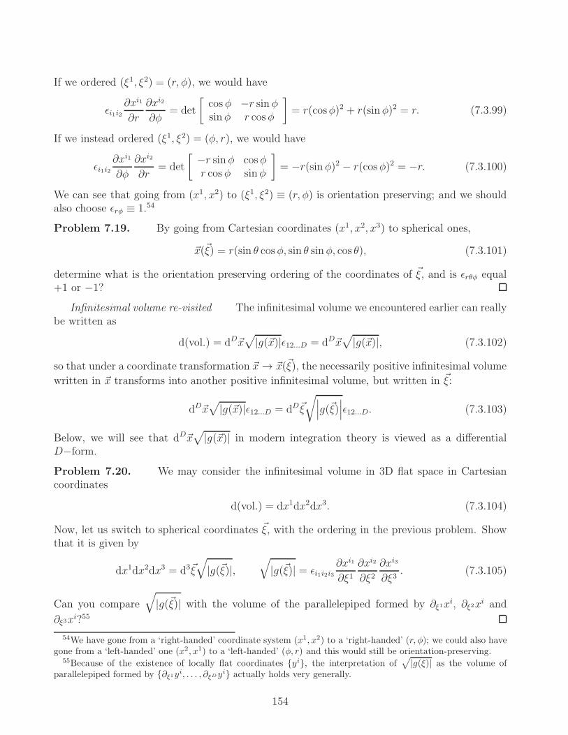
If we ordered (ξ1, ξ2) = (r, φ), we would have

ǫi1i2∂xi1

∂r

∂xi2

∂φ= det

[cos φ −r sin φsinφ r cosφ

]= r(cosφ)2 + r(sinφ)2 = r. (7.3.99)

If we instead ordered (ξ1, ξ2) = (φ, r), we would have

ǫi1i2∂xi1

∂φ

∂xi2

∂r= det

[−r sinφ cosφr cos φ sinφ

]= −r(sinφ)2 − r(cosφ)2 = −r. (7.3.100)

We can see that going from (x1, x2) to (ξ1, ξ2) ≡ (r, φ) is orientation preserving; and we shouldalso choose ǫrφ ≡ 1.54

Problem 7.19. By going from Cartesian coordinates (x1, x2, x3) to spherical ones,

~x(~ξ) = r(sin θ cosφ, sin θ sinφ, cos θ), (7.3.101)

determine what is the orientation preserving ordering of the coordinates of ~ξ, and is ǫrθφ equal+1 or −1?

Infinitesimal volume re-visited The infinitesimal volume we encountered earlier can reallybe written as

d(vol.) = dD~x√|g(~x)|ǫ12...D = dD~x

√|g(~x)|, (7.3.102)

so that under a coordinate transformation ~x → ~x(~ξ), the necessarily positive infinitesimal volume

written in ~x transforms into another positive infinitesimal volume, but written in ~ξ:

dD~x√

|g(~x)|ǫ12...D = dD~ξ

√∣∣∣g(~ξ)∣∣∣ǫ12...D. (7.3.103)

Below, we will see that dD~x√

|g(~x)| in modern integration theory is viewed as a differentialD−form.

Problem 7.20. We may consider the infinitesimal volume in 3D flat space in Cartesiancoordinates

d(vol.) = dx1dx2dx3. (7.3.104)

Now, let us switch to spherical coordinates ~ξ, with the ordering in the previous problem. Showthat it is given by

dx1dx2dx3 = d3~ξ

√|g(~ξ)|,

√|g(~ξ)| = ǫi1i2i3

∂xi1

∂ξ1∂xi2

∂ξ2∂xi3

∂ξ3. (7.3.105)

Can you compare

√|g(~ξ)| with the volume of the parallelepiped formed by ∂ξ1x

i, ∂ξ2xi and

∂ξ3xi?55

54We have gone from a ‘right-handed’ coordinate system (x1, x2) to a ‘right-handed’ (r, φ); we could also havegone from a ‘left-handed’ one (x2, x1) to a ‘left-handed’ (φ, r) and this would still be orientation-preserving.

55Because of the existence of locally flat coordinates yi, the interpretation of√|g(ξ)| as the volume of

parallelepiped formed by ∂ξ1yi, . . . , ∂ξDyi actually holds very generally.

154

Cross-Product in Flat 3D, Right-hand rule Notice the notion of orientation in 3D isclosely tied to the “right-hand rule” in vector calculus. Let ~X and ~Y be vectors in Euclidean3-space. In Cartesian coordinates, where gij = δij, you may check that their cross product is

(~X × ~Y

)k= ǫijkX iY j . (7.3.106)

For example, if ~X is parallel to the positive x1 axis and ~Y parallel to the positive x2-axis, sothat ~X = | ~X|(1, 0, 0) and ~Y = |~Y |(0, 1, 0), the cross product reads

(~X × ~Y

)k→ | ~X||~Y |ǫ12k = | ~X||~Y |δk3 , (7.3.107)

i.e., it is parallel to the positive x3 axis. (Remember k cannot be either 1 or 2 because ǫijk isfully antisymmetric.) If we had chosen ǫ123 = ǫ123 ≡ −1, then the cross product would becomethe “left-hand rule”. Below, I will continue to point out, where appropriate, how this issue oforientation arises in differential geometry.

Problem 7.21. Show that the Levi-Civita tensor with all upper indices is given by

ǫi1i2...iD =sgn det(gab)√

|g|ǫi1i2...iD . (7.3.108)

In curved spaces, the sign of the det gab = 1; whereas in curved spacetimes it depends on thesignature used for the flat metric.56 Hint: Raise the indices by contracting with inverse metrics,then recall the cofactor expansion definition of the determinant.

Problem 7.22. Show that the covariant derivative of the Levi-Civita tensor is zero.

∇j ǫi1i2...iD = 0. (7.3.109)

(Hint: Start by expanding the covariant derivative in terms of Christoffel symbols; then gothrough some combinatoric reasoning or invoke the equivalence principle.) From this, explainwhy the following equalities are true; for some vector V ,

∇j

(ǫi1i2...iD−2jkVk

)= ǫi1i2...iD−2jk∇jVk = ǫi1i2...iD−2jk∂jVk. (7.3.110)

Why is ∇iVj −∇jVi = ∂iVj − ∂jVi for any Vi? Hint: expand the covariant derivatives in termsof the partial derivatives and the Christoffel symbols.

Combinatorics This is an appropriate place to state how to actually construct a fullyantisymmetric tensor from a given tensor Ti1...iN . Denoting Π(i1 . . . iN) to be a permutation ofthe indices i1 . . . iN, the antisymmetrization procedure is given by

T[i1...iN ] =

N !∑

permutations Π of i1,i2,...,iN

σΠ · TΠ(i1...iN ) (7.3.111)

=∑

even permutations Π of i1,i2,...,iN

TΠ(i1...iN ) −∑

odd permutations Π of i1,i2,...,iN

TΠ(i1...iN ).

56See eq. (7.2.51) to understand why the sign of the determinant of the metric is always determined by thesign of the determinant of its flat counterpart.

155

In words: for a rank−N tensor, T[i1...iN ] consists of a sum of N ! terms. The first is Ti1...iN .Each and every other term consists of T with its indices permuted over all the N ! − 1 distinctremaining possibilities, multiplied by σΠ = +1 if it took even number of index swaps to get tothe given permutation, and σΠ = −1 if it took an odd number of swaps. (The σΠ is often calledthe sign of the permutation Π.) For example,

T[ij] = Tij − Tji, T[ijk] = Tijk − Tikj − Tjik + Tjki + Tkij − Tkji. (7.3.112)

Can you see why eq. (7.3.111) yields a fully antisymmetric object? Consider any pair of distinctindices, say ia and ib, for 1 ≤ (a 6= b) ≤ N . Since the sum on its right hand side contains everypermutation (multiplied by the sign) – we may group the terms in the sum of eq. (7.3.111)into pairs, say σΠℓ

Tj1...ia...ib...jN −σΠℓTj1...ib...ia...jN . That is, for a given term σΠℓ

Tj1...ia...ib...jN theremust be a counterpart with ia ↔ ib swapped, multipled by a minus sign, because – if the firstterm involved even (odd) number of swaps to get to, then the second must have involved an odd(even) number. If we now considered swapping ia ↔ ib in every term in the sum on the righthand side of eq. (7.3.111),

T[i1...ia...ib...iN ] = σΠℓTj1...ia...ib...jN − σΠℓ

Tj1...ib...ia...jN + . . . , (7.3.113)

T[i1...ib...ia...iN ] = − (σΠℓTj1...ia...ib...jN − σΠℓ

Tj1...ib...ia...jN + . . . ) . (7.3.114)

Problem 7.23. Given Ti1i2...iN , how do we construct a fully symmetric object from it, i.e.,such that swapping any two indices returns the same object?

Problem 7.24. If the Levi-Civita symbol is subject to the convention ǫ12...D ≡ 1, explainwhy it is equivalent to the following expansion in Kronecker δs.

ǫi1i2...iD = δ1[i1δ2i2. . . δD−1

iD−1δDiD] (7.3.115)

Can you also explain why the following is true?

ǫa1a2...aD−1aD detA = ǫi1i2...iD−1iDAi1a1Ai2

a2. . . A

iD−1

aD−1AiD

aD(7.3.116)

Problem 7.25. Argue that

T[i1...iN ] = T[i1...iN−1]iN − T[iN i2...iN−1]i1 − T[i1iN i3...iN−1]i2 (7.3.117)

−T[i1i2iN i4...iN−1]i3 − · · · − T[i1...iN−2iN ]iN−1.

Product of Levi-Civita tensors The product of two Levi-Civita tensors will be im-portant for the discussions to come. We have

ǫi1...iNk1...kD−N ǫj1...jNk1...kD−N= sgn det(gab) · ANδ

i1[j1. . . δiNjN ], 1 ≤ N ≤ D, (7.3.118)

ǫk1...kD ǫk1...kD = sgn det(gab) · A0, AN≥0 ≡ (D −N)!. (7.3.119)

(Remember 0! = 1! = 1; also, δi1[j1 . . . δiNjN ] = δ

[i1j1. . . δ

iN ]jN

.) Let us first understand why there area bunch of Kronecker deltas on the right hand side, starting from the N = D case – where noindices are contracted.

sgn det(gab)ǫi1...iD ǫj1...jD = ǫi1...iDǫj1...jD = δi1[j1 . . . δ

iDjD] (7.3.120)

156

(This means AD = 1.) The first equality follows from eq. (7.3.108). The second may seem a bitsurprising, because the indices i1, . . . , iD are attached to a completely different ǫ tensor fromthe j1, . . . , jD. However, if we manipulate

δi1[j1 . . . δiDjD] = δi1[1 . . . δ

iDD]σj = δ1[1 . . . δ

DD]σiσj = σiσj = ǫi1...iDǫj1...jD , (7.3.121)

where σi = 1 if it took even number of swaps to re-arrange i1, . . . , iD to 1, . . . , D and σi = −1if it took odd number of swaps; similarly, σj = 1 if it took even number of swaps to re-arrangej1, . . . , jD to 1, . . . , D and σj = −1 if it took odd number of swaps. But σi is precisely theLevi-Civita symbol ǫi1...iD and likewise σj = ǫj1...jD . The (≥ 1)-contractions between the ǫs can, inprinciple, be obtained by contracting the right hand side of (7.3.120). Because one contractionof the (N + 1) Kronecker deltas have to return N Kronecker deltas, by induction, we now seewhy the right hand side of eq. (7.3.118) takes the form it does for any N .

What remains is to figure out the actual value of AN . We will do so recursively, by findinga relationship between AN and AN−1. We will then calculate A1 and use it to generate all thehigher ANs. Starting from eq. (7.3.118), and employing eq. (7.3.117),

ǫi1...iN−1σk1...kD−N ǫj1...jN−1σk1...kD−N= ANδ

i1[j1. . . δ

iN−1

jN−1δσσ] (7.3.122)

= AN

(δi1[j1 . . . δ

iN−1

jN−1]δσσ − δi1[σδ

i2j2. . . δ

iN−1

jN−1]δσj1 − δi1[j1δ

i2σ δ

i3j3. . . δ

iN−1

jN−1]δσj2 − · · · − δi1[j1 . . . δ

iN−2

jN−2δiN−1

σ] δσjN−1

)

= AN · (D − (N − 1))δi1[j1 . . . δiN−1

jN−1]≡ AN−1δ

i1[j1. . . δ

iN−1

jN−1].

(The last equality is a definition, because AN−1 is the coefficient of δi1[j1 . . . δiN−1

jN−1].) We have the

relationship

AN =AN−1

D − (N − 1). (7.3.123)

If we contract every index, we have to sum over all the D! (non-zero components of the Levi-Civita symbol)2,

ǫi1...iD ǫi1...iD = sgn det(gab) ·∑

i1,...,iD

(ǫi1...iD)2 = sgn det(gab) ·D! (7.3.124)

That means A0 = D!. If we contracted every index but one,

ǫik1...kD ǫjk1...kD = sgn det(gab)A1δij . (7.3.125)

Contracting the i and j indices, and invoking eq. (7.3.124),

sgn det(gab) ·D! = sgn det(gab)A1 ·D ⇒ A1 = (D − 1)!. (7.3.126)

That means we may use A1 (or, actually, A0) to generate all other AN≥0s,

AN =AN−1

(D − (N − 1))=

1

D − (N − 1)

AN−2

D − (N − 2)= . . .

=A1

(D − 1)(D − 2)(D − 3) . . . (D − (N − 1))=

(D − 1)!

(D − 1)(D − 2)(D − 3) . . . (D − (N − 1))

157

=(D − 1)(D − 2)(D − 3) . . . (D − (N − 1))(D −N)(D − (N + 1)) . . . 3 · 2 · 1

(D − 1)(D − 2)(D − 3) . . . (D − (N − 1))

= (D −N)!. (7.3.127)

Note that 0! = 1, so AD = 1 as we have found earlier.

Problem 7.26. Matrix determinants revisited Explain why the cofactor expansiondefinition of a square matrix in eq. (3.2.1) can also be expressed as

detA = ǫi1i2...iD−1iDA1i1A2

i2. . . AD−1

iD−1AD

iD(7.3.128)

provided we define ǫi1i2...iD−1iD in the same way we defined its lower index counterpart, includingǫ123...D ≡ 1. That is, why can we cofactor expand about either the rows or the columns of amatrix, to obtain its determinant? What does that tell us about the relation detAT = detA?Can you also prove, using our result for the product of two Levi-Civita symbols, that det(A·B) =(detA)(detB)?

Problem 7.27. In 3D vector calculus, the curl of a gradient of a scalar is zero – how wouldyou express that using the ǫ tensor? What about the statement that the divergence of a curl ofa vector field is zero? Can you also derive, using the ǫ tensor in Cartesian coordinates and eq.(7.3.118), the 3D vector cross product identity

~A× ( ~B × ~C) = ( ~A · ~C) ~B − ( ~A · ~B) ~C? (7.3.129)

Hodge dual We are now ready to define the Hodge dual. Given a fully antisymmetricrank-N tensor Ti1...iN , its Hodge dual – which I shall denote as T j1...jD−N – is a fully antisymmetricrank-(D −N) tensor whose components are

T j1...jD−N ≡ 1

N !ǫj1...jD−N i1...iNTi1...iN . (7.3.130)

Invertible Note that the Hodge dual is an invertible operation, as long as weare dealing with fully antisymmetric tensors, in that given T j1...jD−N we can recoverTi1...iN and vice versa.57 All you have to do is contract both sides with the Levi-Civitatensor, namely

Ti1...iN =(−)N(D−N)

(D −N)!ǫj1...jD−N i1...iN T

j1...jD−N . (7.3.131)

In other words T j1...jD−N and Ti1...iN contain the same amount of information.

Problem 7.28. Using eq. (7.3.118), verify the proportionality constant (−)N(D−N)/(D −N)! in the inverse Hodge dual of eq. (7.3.131), and thereby prove that the Hodge dual is indeedinvertible for fully antisymmetric tensors.

57The fully antisymmetric property is crucial here: any symmetric portion of a tensor contracted with theLevi-Civita tensor would be lost. For example, an arbitrary rank-2 tensor can always be decomposed as Tij =(1/2)Tij + (1/2)T[ij]; then, ǫ

i1...iD−2jkTjk = ǫi1...iD−2jk((1/2)Tjk + (1/2)T[jk]) = (1/2)ǫi1...iD−2jkT[jk]. The

symmetric part is lost because ǫi1...iD−2jkTjk = −ǫi1...iD−2kjTkj.

158

Curl The curl of a vector field Ai can now either be defined as the antisymmetric rank-2tensor

Fij ≡ ∂[iAj] (7.3.132)

or its rank-(D − 2) Hodge dual

F i1i2...iD−2 ≡ 1

2ǫi1i2...iD−2jk∂[jAk]. (7.3.133)

(D = 3)-dimensional space is a special case where both the original vector field Ai and the

Hodge dual F i are rank-1 tensors. This is usually how electromagnetism is taught: that in 3Dthe magnetic field is a vector arising from the curl of the vector potential Ai:

Bk =1

2ǫijk∂[jAk] = ǫijk∂jAk. (7.3.134)

In particular, when we specialize to 3D flat space with Cartesian coordinates:(~∇× ~A

)i= ǫijk∂jAk, (Flat 3D Cartesian). (7.3.135)

(~∇× ~A

)1= ǫ123∂2A3 + ǫ132∂3A2 = ∂2A3 − ∂3A2, etc. (7.3.136)

By setting i = 1, 2, 3 we can recover the usual definition of the curl in 3D vector calculus. Butyou may have noticed from equations (7.3.132) and (7.3.133), in any other dimension, that themagnetic field is really not a (rank−1) vector but should be viewed either as a rank−2 curl ora rank−(D − 2) Hodge dual of this curl.

Divergence versus Curl We can extend the definition of a curl of a vector field to thatof a rank−N fully antisymmetric Bi1...iN as

∇[σBi1...iN ] = ∂[σBi1...iN ]. (7.3.137)

(Can you explain why the ∇ can be replaced with ∂?) With the Levi-Civita tensor, we canconvert the curl of an antisymmetric tensor into the divergence of its dual,

∇σBj1...jD−N−1σ =

1

N !ǫj1...jD−N−1σi1...iN∇σBi1...iN (7.3.138)

= (N + 1) · ǫj1...jD−N−1σi1...iN∂[σBi1...iN ]. (7.3.139)

Problem 7.29. Show, by contracting both sides of eq. (7.3.134) with an appropriate ǫ-tensor, that

ǫijkBk = 2∂[iAj]. (7.3.140)

Assume sgn det(gab) = 1.

Problem 7.30. In D-dimensional space, is the Hodge dual of a rank-D fully antisym-metric tensor Fi1...iD invertible? Hint: If Fi1...iD is fully antisymmetric, how many independent

components does it have? Can you use that observation to relate F and Fi1...iD in

F ≡ 1

D!ǫi1...iDFi1...iD? (7.3.141)

159

Problem 7.31. Curl, divergence and all that The electromagnetism textbook byJ.D.Jackson contains on its very last page explicit forms of the gradient and Laplacian of ascalar as well as divergence and curl of a vector – in Cartesian, cylindrical, and spherical coordi-nates in 3-dimensional flat space. Can you derive them with differential geometric techniques?Note that the vectors there are expressed in an orthonormal basis.

Cartesian coordinates In Cartesian coordinates x1, x2, x3 ∈ R3, we have the metric

dℓ2 = δijdxidxj . (7.3.142)

Show that the gradient of a scalar ψ is

~∇ψ = (∂1ψ, ∂2ψ, ∂3ψ) = (∂1ψ, ∂2ψ, ∂3ψ); (7.3.143)

the Laplacian of a scalar ψ is

∇i∇iψ = δij∂i∂jψ =(∂21 + ∂22 + ∂23

)ψ; (7.3.144)

the divergence of a vector A is

∇iAi = ∂iA

i; (7.3.145)

and the curl of a vector A is

(~∇× ~A)i = ǫijk∂jAk. (7.3.146)

Cylindrical coordinates In cylindrical coordinates ρ ≥ 0, 0 ≤ φ < 2π, z ∈ R, employ thefollowing parametrization for the Cartesian components of the 3D Euclidean coordinate vector

~x = (ρ cosφ, ρ sinφ, z) (7.3.147)

to argue that the flat metric is translated from gij = δij to

dℓ2 = dρ2 + ρ2dφ2 + dz2. (7.3.148)

Show that the gradient of a scalar ψ is

∇ρψ = ∂ρψ, ∇φψ =1

ρ∂φψ, ∇zψ = ∂zψ; (7.3.149)

the Laplacian of a scalar ψ is

∇i∇iψ =1

ρ∂ρ (ρ∂ρψ) +

1

ρ2∂2φψ + ∂2zψ; (7.3.150)

the divergence of a vector A is

∇iAi =

1

ρ

(∂ρ(ρAρ

)+ ∂φA

φ)+ ∂zA

z; (7.3.151)

160

and the curl of a vector A is

ǫρjk∂jAk =1

ρ∂φA

z − ∂zAφ, ǫφjk∂jAk = ∂zA

ρ − ∂ρAz,

ǫzjk∂jAk =1

ρ

(∂ρ

(ρAφ

)− ∂φA

ρ). (7.3.152)

Spherical coordinates In spherical coordinates r ≥ 0, 0 ≤ θ ≤ π, 0 ≤ φ < 2π the Cartesiancomponents of the 3D Euclidean coordinate vector reads

~x = (r sin(θ) cos(φ), r sin(θ) sin(φ), r cos(θ)) . (7.3.153)

Show that the flat metric is now

dℓ2 = dr2 + r2(dθ2 + (sin θ)2dφ2

); (7.3.154)

the gradient of a scalar ψ is

∇rψ = ∂rψ, ∇θψ =1

r∂θψ, ∇φψ =

1

r sin θ∂φψ; (7.3.155)

the Laplacian of a scalar ψ is

∇i∇iψ =1

r2∂r(r2∂rψ

)+

1

r2 sin θ∂θ (sin θ · ∂θψ) +

1

r2(sin θ)2∂2φψ; (7.3.156)

the divergence of a vector A reads

∇iAi =

1

r2∂r(r2Ar

)+

1

r sin θ∂θ

(sin θ ·Aθ

)+

1

r sin θ∂φA

φ; (7.3.157)

and the curl of a vector A is given by

ǫrjk∂jAk =1

r sin θ

(∂θ(sin θ · Aφ)− ∂φA

θ), ǫθjk∂jAk =

1

r sin θ∂φA

r − 1

r∂r(rA

φ),

ǫφjk∂jAk =1

r

(∂r

(rAθ

)− ∂θA

r). (7.3.158)

7.4 Hypersurfaces

7.4.1 Induced Metrics

There are many physical and mathematical problems where we wish to study some (N < D)-dimensional (hyper)surface residing (aka embedded) in aD dimensional ambient space. One wayto describe this surface is to first endow it with N coordinates ξI|I = 1, 2, . . . , N, whose indiceswe will denote with capital letters to distinguish from the D coordinates xi parametrizing the

ambient space. Then the position of the point ~ξ on this hypersurface in the ambient perspective

161

is given by ~x(~ξ). Distances on this hypersurface can be measured using the ambient metric byrestricting the latter on the former, i.e.,

gijdxidxj → gij

(~x(~ξ)

) ∂xi(~ξ)∂ξI

∂xj(~ξ)

∂ξJdξIdξJ ≡ HIJ(~ξ)dξ

IdξJ. (7.4.1)

The HIJ is the (induced) metric on the hypersurface.58

Observe that the N vectors∂xi

∂ξI∂i

∣∣∣∣ I = 1, 2, . . . , N

, (7.4.2)

are tangent to this hypersurface. They form a basis set of tangent vectors at a given point ~x(~ξ),but from the ambient D-dimensional perspective. On the other hand, the ∂/∂ξI themselvesform a basis set of tangent vectors, from the perspective of an observer confined to live on thishypersurface.

Example A simple example is provided by the 2-sphere of radius R embedded in 3D flatspace. We already know that it can be parametrized by two angles ξI ≡ (0 ≤ θ ≤ π, 0 ≤ φ < 2π),such that from the ambient perspective, the sphere is described by

xi(~ξ) = R(sin θ cosφ, sin θ sinφ, cos θ), (Cartesian components). (7.4.3)

(Remember R is a fixed quantity here.) The induced metric on the sphere itself, according toeq. (7.4.1), will lead us to the expected result

HIJ(~ξ)dξIdξJ = R2

(dθ2 + (sin θ)2dφ2

). (7.4.4)

Area of 2D surface in 3D flat space A common vector calculus problem is to give somefunction f(x, y) of two variables, where x and y are to be interpreted as Cartesian coordinates ona flat plane; then proceed to ask what its area is for some specified domain on the (x, y)-plane.We see such a problem can be phrased as a differential geometric one. First, we view f as the zcoordinate of some hypersurface embedded in 3-dimensional flat space, so that

X i ≡ (x, y, z) = (x, y, f(x, y)). (7.4.5)

The tangent vectors (∂X i/∂ξI) are

∂X i

∂x= (1, 0, ∂xf) ,

∂X i

∂y= (0, 1, ∂yf) . (7.4.6)

The induced metric, according to eq. (7.4.1), is given by

HIJ(~ξ)dξIdξJ = δij

(∂X i

∂x

∂Xj

∂x(dx)2 +

∂X i

∂y

∂Xj

∂y(dy)2 + 2

∂X i

∂x

∂Xj

∂ydxdy

),

HIJ(~ξ)·=

[1 + (∂xf)

2 ∂xf∂yf∂xf∂yf 1 + (∂yf)

2

], ξI ≡ (x, y), (7.4.7)

58The Lorentzian signature of curved spacetimes, as opposed to the Euclidean one in curved spaces, complicatesthe study of hypersurfaces in the former. One has to distinguish between timelike, spacelike and null surfaces.For a pedagogical discussion see Eric Poisson’s A Relativist’s Toolkit – in fact, much of the material in thissection is heavily based on its Chapter 3. Note, however, it is not necessary to know General Relativity to studyhypersurfaces in curved spacetimes.

162

where on the second line the “·=” means it is “represented by” the matrix to its right – the

first row corresponds, from left to right, to the xx, xy components; the second row yx and yycomponents. Recall that the infinitesimal volume (= 2D area) is given in any coordinate system

~ξ by d2ξ

√detHIJ(~ξ). That means from taking the det of eq. (7.4.7), if the domain on (x, y) is

denoted as D, the corresponding area swept out by f is given by the 2D integral∫

D

dxdy√detHIJ(x, y) =

∫

D

dxdy√(1 + (∂xf)2)(1 + (∂yf)2)− (∂xf∂yf)2

=

∫

D

dxdy√1 + (∂xf(x, y))2 + (∂yf(x, y))2. (7.4.8)

Differential Forms and Volume Although we have not (and shall not) employ differentialforms very much, it is very much part of modern integration theory. One no longer writes∫d3~xf(~x), for instance, but rather

∫f(~x)dx1 ∧ dx2 ∧ dx3. (7.4.9)

More generally, whenever the following N−form occur under an integral sign, we have thedefinition

dx1 ∧ dx2 ∧ · · · ∧ dxN−1 ∧ dxN︸ ︷︷ ︸(Differential form notation)

≡ dN~x︸︷︷︸Physicists’ colloquial math-speak

. (7.4.10)

(Here N ≤ D, where D is the dimension of space.) This needs to be supplemented with theconstraint that it is a fully antisymmetric object:

dxi1 ∧ dxi2 ∧ · · · ∧ dxiN−1 ∧ dxiN = ǫi1...iNdx1 ∧ dx2 ∧ · · · ∧ dxN−1 ∧ dxN . (7.4.11)

The superposition of rank-(N ≤ D) differential forms spanned by (1/N !)Fi1...iNdxi1∧· · ·∧dxiN,

for arbitrary but fully antisymmetric Fi1...iN, forms a vector space.Why differential forms are fundamental to integration theory is because, it is this antisym-

metry that allows its proper definition as the volume spanned by an N−parallelepiped. For one,the antisymmetric nature of forms is responsible for the Jacobian upon a change-of-variables~x(~y) familiar from multi-variable calculus – using eq. (7.4.11):

dx1 ∧ dx2 ∧ · · · ∧ dxN−1 ∧ dxN =∂x1

∂yi1∂x2

∂yi2. . .

∂xN

∂yiNdyi1 ∧ dyi2 ∧ · · · ∧ dyiN−1 ∧ dyiN

=∂x1

∂yi1∂x2

∂yi2. . .

∂xN

∂yiNǫi1...iNdy1 ∧ dy2 ∧ · · · ∧ dyN−1 ∧ dyN

=

(det

∂xa

∂yb

)dy1 ∧ dy2 ∧ · · · ∧ dyN−1 ∧ dyN . (7.4.12)

In a (D ≥ 2)−dimensional flat space, you might be familiar with the statement that D linearlyindependent vectors define a D−parallelepiped. Its volume, in turn, is computed through thedeterminant of the matrix whose columns (or rows) are these vectors. If we now consider the(N ≤ D)−form built out of N scalar fields ΦI|I = 1, 2, . . . , N, i.e.,

dΦ1 ∧ · · · ∧ dΦN , (7.4.13)

163

let us see how it defines an infinitesimal N−volume by generalizing the notion of volume-as-determinants.59 Focusing on theN = 2 case, if ~v ≡ (p1dx

1, . . . , pDdxD) and ~w ≡ (q1dx

1, . . . , qDdxD)

are two linearly independent vectors formed from pi = ∂iΦ1 and qi = ∂iΦ

2, then

dΦ1 ∧ dΦ2 = (pidxi) ∧ (qjdx

j) = piqjdxi ∧ dxj (7.4.14)

is in fact the 2D area spanned by the parallelepiped defined by ~v and ~w. For, since dΦ1 ∧ dΦ2 isa coordinate scalar, we may choose a locally flat coordinate system yi such that pi and qi lieon the (1, 2)−plane; i.e., pi>2 = qi>2 = 0 and

dΦ1 ∧ dΦ2 = (pidyi) ∧ (qjdy

j) = p1q2dy1 ∧ dy2 + p2q1dy

2 ∧ dy1

= (p1q2 − p2q1)ddx1dx2 = det

[~v ~w

]; (7.4.15)

where now

~v =(∂1Φ

1dy1, ∂2Φ1dy2,~0

), (7.4.16)

~w =(∂1Φ

2dy1, ∂2Φ2dy2,~0

). (7.4.17)

This argument can be readily extended to higher 2 < N ≤ D.

7.4.2 Fluxes, Gauss-Stokes’ theorems, Poincare lemma

Normal to hypersurface Suppose the hypersurface is (D− 1) dimensional, sitting in a Ddimensional ambient space. Then it could also be described by first identifying a scalar functionof the ambient space f(~x) such that some constant-f surface coincides with the hypersurface,

f(~x) = C ≡ constant. (7.4.18)

For example, a 2-sphere of radius R can be defined in Cartesian coordinates ~x as

f(~x) = R2, where f(~x) = ~x2. (7.4.19)

Given the function f , we now show that df = 0 can be used to define a unit normal ni through

ni ≡ ∇if√∇jf∇jf

=gik∂kf√

glm∇lf∇mf. (7.4.20)

That ni is of unit length can be checked by a direct calculation. For ni to be normal to thehypersurface means, when dotted into the latter’s tangent vectors from our previous discussion,it returns zero:

∂xi(~ξ)

∂ξI∂if(~x)

∣∣∣∣∣on hypersurface

=∂

∂ξIf(~x(~ξ)

)= ∂If(~ξ) = 0. (7.4.21)

59These scalar fields ΦI can also be thought of as coordinates parametrizing some N−dimensional sub-spaceof the ambient D−dimensional space.

164

The second and third equalities constitute just a re-statement that f is constant on our hyper-surface. Using ni we can also write down the induced metric on the hypersurface as

Hij = gij − ninj . (7.4.22)

This makes sense as an induced metric on the hypersurface of one lower dimension than that ofthe ambient D-space, because Hij is itself orthogonal to n

i:

Hijnj = (gij − ninj)n

j = ni − ni = 0. (7.4.23)

Any other vector u dotted into the metric will have its n-component subtracted out:

H iju

j =(δij − ninj

)uj = ui − ni(nju

j). (7.4.24)

Problem 7.32. For the 2-sphere in 3-dimensional flat space, defined by eq. (7.4.19), calcu-late the components of the induced metric Hij in eq. (7.4.22) and compare it that in eq. (7.4.4).

Hint: compute d√~x2 in terms of dxi and exploit the constraint ~x2 = R2; then consider what

is the −(nidxi)2 occurring in Hijdx

idxj, when written in spherical coordinates?

Problem 7.33. Consider some 2-dimensional surface parametrized by ξI = (σ, ρ), whosetrajectory in D-dimensional flat space is provided by the Cartesian coordinates ~x(σ, ρ). What isthe formula analogous to eq. (7.4.8), which yields the area of this 2D surface over some domainD on the (σ, ρ) plane? Hint: First ask, “what is the 2D induced metric?” Answer:

Area =

∫

D

dσdρ√

(∂σ~x)2(∂ρ~x)2 − (∂σ~x · ∂ρ~x)2, (∂I~x)2 ≡ ∂Ix

i∂Ixjδij . (7.4.25)

(This is not too far from the Nambu-Goto action of string theory.)

Directed surface elements What is the analog of d ~(Area) from vector calculus? Thisquestion is important for the discussion of the curved version of Gauss’ theorem, as well as thedescription of fluxes – rate of flow of, say, a fluid – across surface areas. If we have a (D − 1)dimensional hypersurface with induced metric HIJ(ξ

K), determinant H ≡ detHIJ, and a unitnormal ni to it, then the answer is

dD−1Σi ≡ dD−1~ξ

√|H(~ξ)|ni

(~x(~ξ)

)(7.4.26)

= dD−1~ξ ǫij1j2...jD−1

(~x(~ξ)

) ∂xj1(~ξ)∂ξ1

∂xj2(~ξ)

∂ξ2. . .

∂xjD−1(~ξ)

∂ξD−1. (7.4.27)

The difference between equations (7.4.26) and (7.4.27) is that the first requires knowing thenormal vector beforehand, while the second description is purely intrinsic to the hypersurfaceand can be computed once its parametrization ~x(~ξ) is provided. Also be aware that the choiceof orientation of the ξI should be consistent with that of the ambient ~x and the infinitesimalvolume dD~x

√|g|ǫ12...D.

The dD−1ξ√|H| is the (scalar) infinitesimal area (= (D − 1)-volume) and ni provides the

direction. The second equality requires justification. Let’s define E iI |I = 1, 2, 3, . . . , D − 1 to

be the (D − 1) vector fields

E iI (~ξ) ≡ ∂xi(~ξ)

∂ξI. (7.4.28)

165

Problem 7.34. Show that the tensor in eq. (7.4.27),

ni ≡ ǫij1j2...jD−1E j11 . . . E jD−1

D−1 (7.4.29)

is orthogonal to all the (D − 1) vectors E iI . Since ni is the sole remaining direction in the D

space, ni must be proportional to ni

ni = ϕ · ni. (7.4.30)

To find ϕ we merely have to dot both sides with ni,

ϕ(~ξ) =

√|g(~x(~ξ))|ǫij1j2...jD−1

ni∂xj1(~ξ)

∂ξ1. . .

∂xjD−1(~ξ)

∂ξD−1. (7.4.31)

Given a point of the surface ~x(~ξ) we can always choose the coordinates ~x of the ambient spacesuch that, at least in a neighborhood of this point, x1 refers to the direction orthogonal to thesurface and the x2, x3, . . . , xD lie on the surface itself. Argue that, in this coordinate system,eq. (7.4.20) becomes

ni =g(i)(1)√g(1)(1)

, (7.4.32)

and therefore eq. (7.4.31) reads

ϕ(~ξ) =

√|g(~x(~ξ))|

√g(1)(1). (7.4.33)

Cramer’s rule (cf. (3.2.12)) from matrix algebra reads: the ij component (the ith row and jthcolumn) of the inverse of a matrix (A−1)ij is ((−)i+j/ detA) times the determinant of A with thejth row and ith column removed. Use this and the definition of the induced metric to concludethat

ϕ(~ξ) =

√|H(~ξ)|, (7.4.34)

thereby proving the equality of equations (7.4.26) and (7.4.27).

Gauss’ theorem We are now ready to state (without proof) Gauss’ theorem. In 3Dvector calculus, Gauss tells us the volume integral, over some domain D, of the divergence of avector field is equal to the flux of the same vector field across the boundary ∂D of the domain.Exactly the same statement applies in a D dimensional ambient curved space with some closed(D − 1) dimensional hypersurface that defines ∂D.

Let V i be an arbitrary vector field, and let ~x(~ξ) describe this closed boundary sur-face so that it has an (outward) directed surface element dD−1Σi given by equations(7.4.26) and (7.4.27). Then

∫

D

dDx√

|g(~x)|∇iVi(~x) =

∫

∂D

dD−1ΣiVi(~x(~ξ)

). (7.4.35)

166

Flux Just as in 3D vector calculus, the dD−1ΣiVi can be viewed as the flux of some fluid

described by V i across an infinitesimal element of the hypersurface ∂D.Remark Gauss’ theorem is not terribly surprising if you recognize the integrand as a totalderivative,

√|g|∇iV

i = ∂i(√

|g|V i) (7.4.36)

(recall eq. (7.3.76)) and therefore it should integrate to become a surface term (≡ (D − 1)-dimensional integral). The right hand side of eq. (7.4.35) merely makes this surface integral

explicit, in terms of the coordinates ~ξ describing the boundary ∂D.Closed surface Note that if you apply Gauss’ theorem eq. (7.4.35), on a closed surfacesuch as the sphere, the result is immediately zero. A closed surface is one where there are noboundaries. (For the 2-sphere, imagine starting with the Northern Hemisphere; the boundary isthen the equator. By moving this boundary south-wards, i.e., from one latitude line to the next,until it vanishes at the South Pole – our boundary-less surface becomes the 2-sphere.) Sincethere are no boundaries, the right hand side of eq. (7.4.35) is automatically zero.

Problem 7.35. We may see this directly for the 2-sphere case. The metric on the 2-sphereof radius R is

dℓ2 = R2(dθ2 + (sin θ)2dφ2), θ ∈ [0, π], φ ∈ [0, 2π). (7.4.37)

Let V i be an arbitrary smooth vector field on the 2-sphere. Show explicitly – namely, do theintegral – that

∫

S2d2x√

|g(~x)|∇iVi = 0. (7.4.38)

Hint: For the φ-integral, remember that φ = 0 and φ = 2π refer to the same point, for a fixedθ.

Problem 7.36. Hudge dual formulation of Gauss’ theorem in D-space. Let usconsider the Hodge dual of the vector field in eq. (7.4.35),

Vi1...iD−1≡ ǫi1...iD−1jV

j . (7.4.39)

First show that

ǫji1...iD−1∇jVi1...iD−1∝ ∂[1V23...D] ∝ ∇iV

i. (7.4.40)

(Find the proportionality factors.) Then deduce the dual formulation of Gauss’ theorem, namely,the relationship between

∫

D

dDx∂[1V23...D] and

∫

∂D

dD−1ξVi1...iD−1

(~x(~ξ)

) ∂xi1(~ξ)∂ξ1

· · · ∂xiD−1(~ξ)

∂ξD−1. (7.4.41)

The Vi1...iD−1∂ξ1x

i1 . . . ∂ξD−1xiD−1 can be viewed as the original tensor Vi1...iD−1, but projected

onto the boundary ∂D.

167

In passing, I should point out, what you have shown in eq. (7.4.41) can be written in acompact manner using differential forms notation:

∫

D

dV =

∫

∂D

V , (7.4.42)

by viewing the fully antisymmetric object V as a differential (D − 1)-form.

Coulomb potential A basic application of Gauss’ theorem is the derivation of the (spher-ically symmetric) Coulomb potential of a unit point charge in D spatial dimensions, satisfying

∇i∇iψ = −δ(D)(~x− ~x′) (7.4.43)

in flat space. Let us consider as domain D the sphere of radius r centered at the point chargeat ~x′. Using spherical coordinates, ~x = rn(~ξ), where n is the unit radial vector emanating from~x′, the induced metric on the boundary ∂D is simply the metric of the (D− 1)-sphere. We nowidentify in eq. (7.4.35) V i = ∇iψ. The normal vector is simply ni∂i = ∂r, and so Gauss’ lawusing eq. (7.4.26) reads

−1 =

∫

SD−1

dD−1~ξ√

|H|rD−1∂rψ(r). (7.4.44)

The∫SD−1 d

D−1~ξ√|H| = 2πD/2/Γ(D/2) is simply the solid angle subtended by the (D−1)-sphere

(≡ volume of the (D − 1)-sphere of unit radius). So at this point we have

∂rψ(r) = − Γ(D/2)

2πD/2rD−1⇒ ψ(r) =

Γ(D/2)

4((D − 2)/2)πD/2rD−2=

Γ(D2− 1)

4πD/2rD−2. (7.4.45)

I have used the Gamma-function identity Γ(z)z = Γ(z+1). Replacing r → |~x−~x′|, we concludethat the Coulomb potential due to a unit strength electric charge is

ψ(~x) =Γ(D

2− 1)

4πD/2|~x− ~x′|D−2. (7.4.46)

It is instructive to also use Gauss’ law using eq. (7.4.27).

−1 =

∫

SD−1

dD−1~ξǫi1...iD−1j∂xi1

∂ξ1· · · ∂x

iD−1

∂ξD−1gjk(~x(~ξ))∂kψ(r ≡

√~x2). (7.4.47)

On the surface of the sphere, we have the completeness relation (cf. (4.3.18)):

gjk(~x(~ξ)) = δIJ∂xj

∂ξI∂xk

∂ξJ+∂xj

∂r

∂xk

∂r. (7.4.48)

(This is also the coordinate transformation for the inverse metric from Cartesian to Sphericalcoordinates.) At this point,

−1 =

∫

SD−1

dD−1~ξǫi1...iD−1j∂xi1

∂ξ1· · · ∂x

iD−1

∂ξD−1

(δIJ∂xj

∂ξI∂xk

∂ξJ+∂xj

∂r

∂xk

∂r

)∂kψ(r ≡

√~x2)

=

∫

SD−1

dD−1~ξǫi1...iD−1j∂xi1

∂ξ1· · · ∂x

iD−1

∂ξD−1

∂xj

∂r

(∂xk

∂r∂kψ(r ≡

√~x2)

). (7.4.49)

168

The Levi-Civita symbol contracted with the Jacobians can now be recognized as simply the

determinant of the D-dimensional metric written in spherical coordinates

√|g(r, ~ξ)|. (Note the

determinant is positive because of the way we ordered our coordinates.) That is in fact equal

to

√|H(r, ~ξ)| because grr = 1. Whereas (∂xk/∂r)∂kψ = ∂rψ. We have therefore recovered the

previous result using eq. (7.4.26).Tensor elements Suppose we have a (N < D)-dimensional domain D parametrized by

~x(ξI)|I = 1, 2, . . . , N whose boundary ∂D is parametrized by ~x(θA)|A = 1, 2, . . . , N − 1. Wemay define a (D −N)-tensor element that generalizes the one in eq. (7.4.27)

dNΣi1...iD−N≡ dNξ ǫi1...iD−N j1j2...jN

(~x(~ξ)

) ∂xj1(~ξ)∂ξ1

∂xj2(~ξ)

∂ξ2. . .

∂xjN (~ξ)

∂ξN. (7.4.50)

We may further define the boundary surface element

dN−1Σi1...iD−Nk ≡ dN−1θ ǫi1...iD−Nkj1...jN−1

(~x(~θ)

) ∂xj1(~θ)∂θ1

∂xj2(~θ)

∂θ2. . .

∂xjN−1(~θ)

∂θN−1. (7.4.51)

Stokes’ theorem60 Stokes’ theorem is the assertion that, in a (N < D)-dimensional simply connected subregion D of some D-dimensional ambient space,the divergence of a fully antisymmetric rank (D − N + 1) tensor field Bi1...iD−Nk

integrated over the domain D can also be expressed as the integral of Bi1...iD−Nk overits boundary ∂D. Namely,

∫

D

dNΣi1...iD−N∇kB

i1...iD−Nk =1

D −N + 1

∫

∂D

dN−1Σi1...iD−NkBi1...iD−Nk, (7.4.52)

N < D, B[i1...iD−Nk] = (D −N + 1)!Bi1...iD−Nk.

Problem 7.37. Hodge dual formulation of Stokes’ theorem. Define

Bj1...jN−1≡ 1

(D −N + 1)!ǫj1...jN−1i1...iD−NkB

i1...iD−Nk. (7.4.53)

Can you convert eq. (7.4.52) into a relationship between

∫

D

dN~ξ∂[i1Bi2...iN ]∂xi1

∂ξ1. . .

∂xiN

∂ξNand

∫

∂D

dN−1~θBi1...iN−1

∂xi1

∂θ1. . .

∂xiN−1

∂θN−1? (7.4.54)

Furthermore, explain why the Jacobians can be “brought inside the derivative”.

∂[i1Bi2...iN ]∂xi1

∂ξ1. . .

∂xiN

∂ξN=∂xi1

∂ξ[1∂|i1|

(∂xi2

∂ξ2. . .

∂xiN

∂ξN ]Bi2...iN

). (7.4.55)

The | · | around i1 indicate it is not to be part of the anti-symmetrization; only do so for theξ-indices.

60Just like for the Gauss’ theorem case, in equations (7.4.50) and (7.4.51), the ~ξ and ~θ coordinate systems needto be defined with orientations consistent with the ambient dD~x

√|g(~x)|ǫ12...D one.

169

Like for Gauss’ theorem, we point out that – by viewing Bj1...jN−1as components of a (N−1)-

form, Stokes’ theorem in eq. (7.4.52) reduces to the simple expression

∫

D

dB =

∫

∂D

B. (7.4.56)

Relation to 3D vector calculus Stokes’ theorem in vector calculus states that the flux of thecurl of a vector field over some 2D domain D sitting in the ambient 3D space, is equal to theline integral of the same vector field along the boundary ∂D of the domain. Because eq. (7.4.52)may not appear, at first sight, to be related to the Stokes’ theorem from 3D vector calculus, weshall work it out in some detail.

Problem 7.38. Consider some 2D hypersurface D residing in a 3D curved space. Forsimplicity, let us foliate D with constant ρ surfaces; let the other coordinate be φ, so ~x(0 ≤ ρ ≤ρ>, 0 ≤ φ ≤ 2π) describes a given point on D and the boundary ∂D is given by the closed loop~x(ρ = ρ>, 0 ≤ φ ≤ 2π). Let

Bik ≡ ǫikjAj (7.4.57)

for some vector field Aj . This implies in Cartesian coordinates,

∇kBik =

(~∇× ~A

)i. (7.4.58)

Denote ~ξ = (ρ, φ). Show that Stokes’ theorem in eq. (7.4.52) reduces to the N = 2 vectorcalculus case:

∫ ρ>

0

dρ

∫ 2π

0

dφ

√|H(~ξ)|~n ·

(~∇× ~A

)=

∫ 2π

0

dφ∂~x(ρ>, φ)

∂φ· ~A(~x(ρ>, φ)). (7.4.59)

where the unit normal vector is given by

~n =(∂~x(~ξ)/∂ρ)× (∂~x(~ξ)/∂φ)∣∣∣(∂~x(~ξ)/∂ρ)× (∂~x(~ξ)/∂φ)

∣∣∣. (7.4.60)

Of course, once you’ve verified Stokes’ theorem for a particular coordinate system, you know bygeneral covariance it holds in any coordinate system, i.e.,

∫

D

d2ξ

√|H(~ξ)|niǫ

ijk∂jAk =

∫

∂D

Aidxi. (7.4.61)

Step-by-step guide: Start with eq. (7.4.27), and show that in a Cartesian basis,

d2Σi = d2ξ

(∂~x

∂ρ× ∂~x

∂φ

)i

. (7.4.62)

170

The induced metric on the 2D domain D is

HIJ = δij∂Ixi∂Jx

j . (7.4.63)

Work out its determinant. Then work out

|(∂~x/∂ρ)× (∂~x/∂φ)|2 (7.4.64)

using the identity

ǫijkǫlmk = δilδjm − δimδ

jl . (7.4.65)

Can you thus relate

√|H(~ξ)| to |(∂~x/∂ρ)× (∂~x/∂φ)|, and thereby verify the left hand side of

eq. (7.4.52) yields the left hand side of (7.4.59)?For the right hand side of eq. (7.4.59), begin by arguing that the boundary (line) element in

eq. (7.4.51) becomes

dΣki = dφ ǫkij∂xj

∂φ. (7.4.66)

Then use ǫij1j2 ǫkj1j2 = 2δik to then show that the right hand side of eq. (7.4.52) is now that ofeq. (7.4.59).

Problem 7.39. Discuss how the tensor element in eq. (7.4.50) transforms under a change

of hypersurface coordinates ~ξ → ~ξ(~ξ′). Do the same for the tensor element in eq. (7.4.51): how

does it transforms under a change of hypersurface coordinates ~θ → ~θ(~θ′)?

Poincare Lemma In 3D vector calculus you have learned that a vector ~B is divergence-less everywhere in space iff it is the curl of another vector ~A.

~∇ · ~B = 0 ⇔ ~B = ~∇× ~A. (7.4.67)

And, the curl of a vector ~B is zero everywhere in space iff it is the gradient of scalar ψ.

~∇× ~B = 0 ⇔ ~B = ~∇ψ. (7.4.68)

Here, we shall see that these statements are special cases of the following.

Poincare lemma In an arbitrary D dimensional curved space, let Bi1...iN (~x)be a fully antisymmetric rank-N tensor field, with N ≤ D. Then, everywhere withina simply connected region of space,

Bi1...iN = ∂[i1Ci2...iN ], (7.4.69)

– i.e., B is the “curl” of a fully antisymmetric rank-(N − 1) tensor C – if and only if

∂[jBi1...iN ] = 0. (7.4.70)

In differential form notation, by treating C as a (N − 1)-form and B as a N -form,Poincare would read: throughout a simply connected region of space,

dB = 0 iff B = dC. (7.4.71)

171

Example I: Electromagnetism Let us recover the 3D vector calculus statement above, thatthe divergence-less nature of the magnetic field is equivalent to it being the curl of some vectorfield. Consider the dual of the magnetic field Bi:

Bij ≡ ǫijkBk. (7.4.72)

The Poincare Lemma says Bij = ∂[iAj] if and only if ∂[kBij] = 0 everywhere in space. We shallproceed to take the dual of these two conditions. Via eq. (7.3.118), the first is equivalent to

ǫkijBij = ǫkij∂[iAj],

= 2ǫkij∂iAj. (7.4.73)

On the other hand, employing eq. (7.3.118),

ǫkijBij = ǫkij ǫijlBl = 2Bk; (7.4.74)

and therefore ~B is the curl of Ai:

Bk = ǫkij∂iAj (7.4.75)

While the latter condition dB = 0 is, again utilizing eq. (7.3.118), equivalent to

0 = ǫkij∂kBij

= ǫkij ǫijl∇kBl = 2∇lB

l. (7.4.76)

That is, the divergence of ~B is zero.Example II A simple application is that of the line integral

I(~x, ~x′;P) ≡∫

P

Aidxi, (7.4.77)

where P is some path in D-space joining ~x′ to ~x. Poincare tells us, if ∂[iAj] = 0 everywhere inspace, then Ai = ∂iϕ, the Ai is a gradient of a scalar ϕ. Then Aidx

i = ∂iϕdxi = dϕ, and the

integral itself is actually path independent – it depends only on the end points:

∫ ~x

~x′Aidx

i =

∫

P

dϕ = ϕ(~x)− ϕ(~x′), whenever ∂[iAj] = 0. (7.4.78)

Problem 7.40. Make a similar translation, from the Poincare Lemma, to the 3D vectorcalculus statement that a vector B is curl-less if and only if it is a pure gradient everywhere.

Problem 7.41. Consider the vector potential, written in 3D Cartesian coordinates,

Aidxi =

x1dx2 − x2dx1

(x1)2 + (x2)2. (7.4.79)

Can you calculate

Fij = ∂[iAj]? (7.4.80)

172

Consider a 2D surface whose boundary ∂D circle around the (0, 0,−∞ < x3 < +∞) line once.Can you use Stokes’ theorem to show that

Fij = 2πǫij3δ(x1)δ(x2)? (7.4.81)

Hint: Convert from Cartesian to polar coordinates (x, y, z) = (r cosφ, r sinφ, z); the line integralon the right hand side of eq. (7.4.61) should simplify considerably. This problem illustrates thesubtlety regarding the “simply connected” requirement of the Poincare lemma. The magneticfield Fij here describes that of a highly localized solenoid lying along the z-axis; its correspondingvector potential is a pure gradient in any simply connected 3−volume not containing the z-axis,but it is no longer a pure gradient in say a solid torus region encircling (but still not containing)it.

173

8 Differential Geometry In Curved Spacetimes

We now move on to differential geometry in curved spacetimes. I assume the reader is familiarwith basic elements of Special Relativity and with the discussion in §(7) – in many instances,I will simply bring over the results from there to the curved spacetime context. In §(8.1) Idiscuss Lorentz/Poincare symmetry in flat spacetime, since it is fundamental to both Specialand General Relativity. I then cover curved spacetime differential geometry proper from §(8.2)through §(8.4), focusing on issues not well developed in §(7). These three sections, together with§(7), are intended to form the first portion – the kinematics of curved space(time)s part61 – ofa course on gravitation. Following that, §(8.5) contains somewhat specialized content regardingthe expansion of geometric quantities off some fixed ‘background’ geometry; and finally, in §(8.6)we compile conformal transformation properties of geometric objects.

8.1 Poincare and Lorentz symmetry

Poincare and Lorentz symmetries play fundamental roles in our understanding of both classicalrelativistic physics and quantum theories of elementary particle interactions. In this section, weshall study it in some detail.

The metric of flat spacetime is, in Cartesian coordinates xµ,

ds2 ≡ ηµνdxµdxν , (8.1.1)

ηµν ≡ diag[1,−1, . . . ,−1]. (8.1.2)

Strictly speaking we should be writing eq. (8.2.1) in the ‘dimensionally-correct’ form

ds2 = c2dt2 − d~x · d~x; (8.1.3)

where c is the speed of light and [ds2] = [Length2]. However, as explained in §(C), since thespeed of light shows up frequently in relativity and gravitational physics, it is often advantageousto set c = 1, which in turn means all speeds are measured using c as the base unit. (v = 0.23would mean v = 0.23c, for instance.) We shall do so throughout this section.

Notice too, we have switched from Latin/English alphabets in §(7), say i, j, k, · · · ∈ 1, 2, 3, . . . , Dto Greek ones µ, ν, · · · ∈ 0, 1, 2, . . . , D ≡ d − 1; the former run over the spatial coordinateswhile the latter over time (0th) and space (1, . . . , D). Also note that the opposite ‘mostly plus’sign convention ηµν = diag[−1,+1, . . . ,+1] is equally valid and, in fact, more popular in thecontemporary physics literature.

We shall define Poincare transformations62 x(x′) to be the set of all coordinate transforma-tions that leave the flat spacetime metric invariant:

ds2 = ηµνdxµdxν = ηα′β′dx′αdx′β . (8.1.4)

As we will now proceed to demonstrate, the most general invertible Poincare transformation is

xµ = aµ + Λµνx

′ν , (8.1.5)

61As opposed to the dynamics of spacetime, which involves studying General Relativity, Einstein’s field equa-tions for the metric, and its applications.

62Poincare transformations are also sometimes known as inhomogeneous Lorentz transformations.

174

where aµ is a constant vector describing a spacetime translation; and Λµν is an arbitrary

(spacetime-constant) Lorentz transformation, which in turn is defined as one that leaves ηµνinvariant in the following manner:

ΛµαΛ

νβηµν = ηαβ. (8.1.6)

Derivation of eq. (8.1.4)63 Now, under a coordinate transformation, eq. (8.1.4) reads

ηµνdxµdxν = ηµν

∂xµ

∂x′α∂xν

∂x′βdx′αdx′β = ηα′β′dx′αdx′β . (8.1.7)

Let us differentiate both sides of eq. (8.1.7) with respect to x′σ.

ηµν∂2xµ

∂x′σ∂x′α∂xν

∂x′β+ ηµν

∂xµ

∂x′α∂2xν

∂x′σ∂x′β= 0. (8.1.8)

Next, consider symmetrizing σα and anti-symmetrizing σβ.

2ηµν∂2xµ

∂x′σ∂x′α∂xν

∂x′β+ ηµν

∂xµ

∂x′α∂2xν

∂x′σ∂x′β+ ηµν

∂xµ

∂x′σ∂2xν

∂x′α∂x′β= 0 (8.1.9)

ηµν∂2xµ

∂x′σ∂x′α∂xν

∂x′β− ηµν

∂2xµ

∂x′β∂x′α∂xν

∂x′σ= 0 (8.1.10)

Since partial derivatives commute, the second term from the left of eq. (8.1.8) vanishes uponanti-symmetrization of σβ. Adding equations (8.1.9) and (8.1.10) hands us

3ηµν∂2xµ

∂x′σ∂x′α∂xν

∂x′β+ ηµν

∂xµ

∂x′α∂2xν

∂x′σ∂x′β= 0. (8.1.11)

Finally, subtracting eq. (8.1.8) from eq. (8.1.11) produces

2ηµν∂2xµ

∂x′σ∂x′α∂xν

∂x′β= 0. (8.1.12)

Because we have assumed Poincare transformations are invertible, we may contract both sideswith ∂x′β/∂xκ.

ηµν∂2xµ

∂x′σ∂x′α∂xν

∂x′β∂x′β

∂xκ= ηµν

∂2xµ

∂x′σ∂x′αδνκ = 0. (8.1.13)

Finally, we contract both sides with ηκρ:

ηµ′κ′ηκ′ρ ∂2xµ

∂x′σ∂x′α=

∂2xρ

∂x′σ∂x′α= 0. (8.1.14)

In words: since the second x′-derivative of x has to vanish, the transformation from x to x′ canat most go linearly as x′; it cannot involve higher powers of x′. This implies the form in eq.(8.1.5). Plugging eq. (8.1.5) the latter into eq. (8.1.7), we recover the necessary definition ofthe Lorentz transformation in eq. (8.1.6).

63This argument can be found in Weinberg [13].

175

The most general invertible coordinate transformations that leave the CartesianMinkowski metric invariant involve the (spacetime-constant) Lorentz transformationsΛµ

α of eq (8.1.6) plus constant spacetime translations.

(Homogeneous) Lorentz Transformations form a Group If Λµα and Λ′µ

α denotesdifferent Lorentz transformations, then notice the composition

Λ′′µα ≡ Λµ

σΛ′σα (8.1.15)

is also a Lorentz transformation. For, keeping in mind the fundamental definition in eq. (8.1.6),we may directly compute

Λ′′µαΛ

′′νβηµν = Λµ

σΛ′σαΛ

νρΛ

′ρβηµν

= Λ′σαΛ

′ρβησρ = ηαβ . (8.1.16)

To summarize:

The set of all Lorentz transformations Λµα satisfying eq. (8.1.6), together with

the composition law in eq. (8.1.15) for defining successive Lorentz transformations,form a Group.

Proof Let Λµα, Λ

′µα and Λ′′µ

α denote distinct Lorentz transformations.

• Closure Above, we have just verified that applying successive Lorentz transforma-tions yields another Lorentz transformation; for e.g., Λµ

σΛ′σν and Λµ

σΛ′σρΛ

′′ρν are Lorentz

transformations.

• Associativity Because applying successive Lorentz transformations amount to matrixmultiplication, and since the latter is associative, that means Lorentz transformations areassociative:

Λ · Λ′ · Λ′′ = Λ · (Λ′ · Λ′′) = (Λ · Λ′) · Λ′′. (8.1.17)

• Identity δµα is the identity Lorentz transformation:

δµσΛσν = Λµ

σδσν = Λµ

ν , (8.1.18)

and

δµαδνβηµν = ηαβ . (8.1.19)

• Inverse Let us take the determinant of both sides of eq. (8.1.6) – by viewing the latteras matrix multiplication, we have ΛT · η · Λ = η, which in turn means

(det Λ)2 = 1 ⇒ det Λ = ±1. (8.1.20)

Here, we have recalled detAT = detA for any square matrix A. Since the determinant ofΛ is strictly non-zero, what eq. (8.1.20) teaches us is that Λ is always invertible: Λ−1 is

176

guaranteed to exist. What remains is to check that, if Λ is a Lorentz transformation, so isΛ−1. Starting with the matrix form of eq. (8.1.6), and utilizing (Λ−1)T = (ΛT )−1,

ΛTηΛ = η (8.1.21)

(ΛT )−1ΛTηΛΛ−1 = (ΛT )−1 · η · Λ−1 (8.1.22)

η = (Λ−1)T · η · Λ−1. (8.1.23)

Lorentzian ‘inner product’ is preserved That Λ is a Lorentz transformation meansit is a linear operator that preserves the Lorentzian inner product. For suppose v and w arearbitrary vectors, the inner product of v′ ≡ Λv and w′ ≡ Λw is that between v and w.

v′ · w′ ≡ ηαβv′αw′β = ηαβΛ

αµΛ

βνv

µwν (8.1.24)

= ηµνvµwν = v · w. (8.1.25)

This is very much analogous to rotations in RD being the linear transformations that preservethe Euclidean inner product between spatial vectors: ~v · ~w = ~v′ · ~w′ for all RT R = ID×D, where~v′ ≡ R~v and ~w′ ≡ R ~w.

Problem 8.1. 4D Lorentz Group and SL2,C Define σµ to be the basis set of 2 × 2complex matrices formed by the 2× 2 identity matrix together with the Pauli matrices, namely

σ0 ≡[1 00 1

], σ1 ≡

[0 11 0

], σ2 ≡

[0 −ii 0

], σ3 ≡

[1 00 −1

]. (8.1.26)

Now let pµ ≡ (p0, p1, p2, p3) be a 4-component collection of real numbers, and verify that

det pµσµ = ηµνpµpν ≡ p2. (8.1.27)

Next, consider the following transformation,

pµσµ → L† · pµσµ · L, (8.1.28)

where L is some arbitrary 2× 2 complex matrix. (This transformation preserves the Hermitiannature of pµσ

µ for real pµ.) Then consider taking their determinant:

det[pµσµ] → det

[L† · pµσµ · L

](8.1.29)

What property must L obey in order that this leaves the determinant invariant, i.e.,

det[pµσµ] = det

[L† · pµσµ · L

]= p2? (8.1.30)

Argue that the set of all L’s obeying eq. (8.1.30), with | detL| = 1 (this is the ‘S’≡‘special’ inSL2,C), forms a group.

We wish to study in some detail what the most general form Λµα may take. To this end, we

shall do so by examining how it acts on some arbitrary vector field vµ. Even though this sectiondeals with Minkowski spacetime, this vµ may also be viewed as a vector in a curved spacetimewritten in an orthonormal basis.

177

Rotations Let us recall that any spatial vector vi may be rotated to point along the1−axis while preserving its Euclidean length. That is, there is always a R, obeying RT R = I

such that

Rijv

j=± |~v|(1, 0, . . . , 0)T , |~v| ≡√δijvivj . (8.1.31)

64Conversely, since R is necessarily invertible, any spatial vector vi can be obtained by rotatingit from |~v|(1,~0T ). Moreover, in D + 1 notation, these rotation matrices can be written as

Rµν=

[1 ~0T

~0 Rij

](8.1.32)

R0νv

ν = v0, (8.1.33)

Riνv

ν = Rijv

j = (±|~v|, 0, . . . , 0)T . (8.1.34)

These considerations tell us, if we wish to study Lorentz transformations that are not rotations,we may reduce their study to the (1 + 1)D case. To see this, we first observe that

Λ

v0

v1

...vD

= Λ

[1 ~0T

~0 R

]

v0

±|~v|~0

. (8.1.35)

And if the result of this matrix multiplication yields non-zero spatial components, namely(v′0, v′1, . . . , v′D)T , we may again find a rotation matrix R′ such that

Λ

v0

v1

...vD

=

v′0

v′1

...v′D

=

[1 ~0T

~0 R′

]

v′0

±|~v′|~0

. (8.1.36)

At this point, we have reduced our study of Lorentz transformations to

[1 ~0T

~0 R′T

]Λ

[1 ~0T

~0 R

]v0

v1

~0

≡ Λ′

v0

v1

~0

=

v′0

v′1

~0

. (8.1.37)

Because Λ was arbitrary so is Λ′, since one can be gotten from another via rotations.Time Reversal & Parity Flips Suppose the time component of the vector vµ were

negative (v0 < 0), we may write it as[−|v0|~v

]= T

[|v0|~v

], T ≡

[−1 ~0T

~0 ID×D

]; (8.1.38)

where T is the time reversal matrix since it reverses the sign of the time component of the vector.You may readily check that T itself is a Lorentz transformation in that it satisfies T TηT = η.

64This R is not unique: for example, by choosing another rotation matrix R′′ that only rotates the spaceorthogonal to vi, RR′′~v and R~v both yield the same result.

178

Problem 8.2. Parity flip of the ith axis Suppose we wish to flip the sign of the ith spatialcomponent of the vector, namely vi → −vi. You can probably guess, this may be implementedvia the diagonal matrix with all entries set to unity, except the ith component – which is setinstead to −1.

iPµνv

ν = vµ, µ 6= i, (8.1.39)

iPiνv

ν = −vi, (8.1.40)

iP ≡ diag[1, 1, . . . , 1, −1︸︷︷︸(i+1)th component

, 1, . . . , 1]. (8.1.41)

Define the rotation matrix Rµν such that it leaves all the axes orthogonal to the 1st and ith

invariant, namely

Rµν e

νℓ = eνℓ , (8.1.42)

eµℓ ≡ δµℓ , ℓ 6= 1, i; (8.1.43)

while rotating the (1, i)-plane clockwise by π/2:

R · e1 = −ei, R · ei = +e1. (8.1.44)

Now argue that

iP = RT · 1P · R. (8.1.45)

Is iP a Lorentz transformation?

Lorentz Boosts As already discussed, we may focus on the 2D case to elucidate theform of the most general Lorentz boost. This is the transformations that would mix time andspace components, and yet leave the metric of spacetime ηµν = diag[1,−1] invariant. (Neithertime reversal, parity flips, nor spatial rotations mix time and space.) This is what revolutionizedhumanity’s understanding of spacetime at the beginning of the 1900’s: inspired by the fact thatthe speed of light is the same in all inertial frames, Einstein discovered Special Relativity, thatthe space and time coordinates of one frame have to become intertwined when being translatedto those in another frame. We will turn this around later when discussing Maxwell’s equations:the constancy of the speed of light in all inertial frames is in fact a consequence of the Lorentzcovariance of the former.

Problem 8.3. We wish to find a 2×2 matrix Λ that obeys ΛT ·η ·Λ = η, where ηµν = diag[1,−1].By examining the diagonal terms of ΛT · η · Λ = η, show that

Λ=

[σ1 cosh(ξ1) σ2 sinh(ξ2)σ3 sinh(ξ1) σ4 cosh(ξ2)

], (8.1.46)

where the σ1,2,3,4 are either +1 or−1; altogether, there are 16 choices of signs. (Hint: x2−y2 = c2,for constant c, describes a hyperbola on the (x, y) plane.) From the off diagonal terms ofΛT · η · Λ = η, argue that either ξ1 = ξ2 ≡ ξ or ξ1 = −ξ2 ≡ ξ. Then explain why, if Λ0

0 were not

179

positive, we can always multiply it by a time reversal matrix to render it so; and likewise Λ11

can always be rendered positive by multiplying it by a parity flip. By requiring Λ00 and Λ1

1 beboth positive, therefore, prove that the resulting 2D Lorentz boost is

Λµν(ξ) =

[cosh(ξ) sinh(ξ)sinh(ξ) cosh(ξ)

]. (8.1.47)

This ξ is known as rapidity. In 2D, the rotation matrix is

Rij(θ) =

[cos(θ) − sin(θ)sin(θ) cos(θ)

]; (8.1.48)

and therefore rapidity ξ is to the Lorentz boost in eq. (8.1.47) what the angle θ is to rotation

Rij(θ) in eq. (8.1.48).

2D Lorentz Group: In (1+1)D, the continuous boost in Λµν(ξ) in eq. (8.1.47),

the continuous rotation Rij(θ) in eq. (8.1.48); and the discrete time reversal and

spatial reflection operators

T =

[−1 00 1

]and P =

[1 00 −1

]; (8.1.49)

altogether form the full set of Lorentz transformations – i.e., all solutions to eq.(8.2.3) consist of products of these 4 matrices.

To understand the meaning of the rapidity ξ, let us consider applying it to an arbitrary 2Dvector Uµ.

U ′ ≡ Λ · U =

[U0 cosh(ξ) + U1 sinh(ξ)U1 cosh(ξ) + U0 sinh(ξ)

]. (8.1.50)

Lorentz Boost: Timelike case Suppose U were timelike, U2 > 0 ⇒ (U0)2 > (U1)2 ⇒|U0/U1| > 1. Then it is not possible to find a finite ξ such that U ′0 = 0, because that wouldamount to solving tanh(ξ) = −U0/U1 but tanh lies between −1 and +1 while −U0/U1 is eitherless than −1 or greater than +1. On the other hand, it does mean we may solve for ξ thatwould set the spatial component to zero: tanh(ξ) = −U1/U0. Recall that tangent vectors maybe interpreted as the derivative of the spacetime coordinates with respect to some parameter λ,namely Uµ ≡ dxµ/dλ. Therefore

U1

U0=

dx1

dλ

dλ

dx0=

dx1

dx0≡ v (8.1.51)

is the velocity associated with Uµ in the frame xµ. Starting from tanh(ξ) = −v, some algebrawould then hand us (cf. eq. (8.1.47))

cosh(ξ) = γ ≡ 1√1− v2

, (8.1.52)

sinh(ξ) = −γ · v = − v√1− v2

, (8.1.53)

Λµν =

[γ −γ · v

−γ · v γ

]. (8.1.54)

180

This in turn yields

U ′ =(sgn(U0)

√ηµνUµUν , 0

)T; (8.1.55)

leading us to interpret the Λµν we have found in eq. (8.1.54) as the boost that bring observers

to the frame where the flow associated with Uµ is ‘at rest’. (Note that, if Uµ = dxµ/dτ , whereτ is proper time, then ηµνU

µUν = 1.)As an important aside, we may generalize the two-dimensional Lorentz boost in eq. (8.1.54)

to D−dimensions. One way to do it, is to simply append to the 2D Lorentz-boost matrix a(D−2)× (D−2) identity matrix (that leaves the 2− through D−spatial components unaltered)in a block diagonal form:

Λµν

?=

γ −γ · v 0−γ · v γ 0

0 0 I(D−2)×(D−2)

. (8.1.56)

But this is not doing much: we are still only boosting in the 1−direction. What if we wish toboost in vi direction, where vi is now some arbitrary spatial vector? To this end, we may promotethe (0, 1) and (1, 0) components of eq. (8.1.54) to the spatial vectors Λ0

i and Λi0 parallel to vi.

Whereas the (1, 1) component of eq. (8.1.54) is to be viewed as acting on the 1D space parallel tovi, namely the operator vivj/~v2. (As a check: When vi = v(1,~0), vivj/~v2 = δi1δ

j1.) The identity

operator acting on the orthogonal (D− 2)× (D− 2) space, i.e., the analog of I(D−2)×(D−2) in eq.(8.1.56), is Πij = δij − vivj/~v2. (Notice: Πijvj = (δij − vivj/~v2)vj = 0.) Altogether, the Lorentzboost in the vi direction is given by

Λµν(~v)=

[γ −γvi

−γvi γ vivj

~v2+(δij − vivj

~v2

)], ~v2 ≡ δabv

abb. (8.1.57)

It may be worthwhile to phrase this discussion in terms of the Cartesian coordinates xµ andx′µ parametrizing the two inertial frames. What we have shown is that the Lorentz boost ineq. (8.1.57) describes

U ′µ = Λµν(~v)U

ν , (8.1.58)

Uµ =dxµ

dλ, U ′µ =

dx′µ

dλ=(sgn(U0)

√ηµνUµUν , 0

)T. (8.1.59)

λ is the intrinsic 1D coordinate parametrizing the worldlines, and by definition does not alterunder Lorentz boost. The above statement is therefore equivalent to

dx′µ = Λµν(~v)dx

ν , (8.1.60)

x′µ = Λµν(~v)x

ν + aµ, (8.1.61)

where the spacetime translation aµ shows up here as integration constants.

Problem 8.4. Lorentz boost in (D + 1)−dimensions If vµ ≡ (1, vi), check via a di-rection calculation that the Λµ

ν in eq. (8.1.57) produces a Λµνv

ν that has no non-trivial spa-tial components. Also check that eq. (8.1.57) is, in fact, a Lorentz transformation. What isΛµ

σ(~v)Λσν(−~v)?

181

Lorentz Boost: Spacelike case Suppose U were spacelike, U2 < 0 ⇒ (U0)2 <(U1)2 ⇒ |U1/U0| = |dx1/dx0| ≡ |v| > 1. Then, recalling eq. (8.1.50), it is not possible to find afinite ξ such that U ′1 = 0, because that would amount to solving tanh(ξ) = −U1/U0, but tanhlies between −1 and +1 whereas −U1/U0 = −v is either less than −1 or greater than +1. Onthe other hand, it is certainly possible to have U ′0 = 0. Simply do tanh(ξ) = −U0/U1 = −1/v.Similar algebra to the timelike case then hands us

cosh(ξ) =(1− v−2

)−1/2=

|v|√v2 − 1

, (8.1.62)

sinh(ξ) = −(1/v)(1− v−2

)−1/2= − sgn(v)√

v2 − 1, (8.1.63)

U ′ =(0, sgn(v)

√−ηµνUµUν

)T, v ≡ U1

U0. (8.1.64)

We may interpret U ′µ and Uµ as infinitesimal vectors joining the same pair of spacetime pointsbut in their respective frames. Specifically, U ′µ are the components in the frame where the pairlies on the same constant-time surface (U ′0 = 0). While Uµ are the components in a boostedframe.

Lorentz Boost: Null (aka lightlike) case If U were null, that means (U0)2 = (U1)2,which in turn means

Uµ = ω(1,±1) (8.1.65)

for some real number ω. Upon a Lorentz boost, eq. (8.1.50) tells us

U ′ ≡ Λ · U = ω

[cosh(ξ)± sinh(ξ)sinh(ξ)± cosh(ξ)

]. (8.1.66)

As we shall see below, if Uµ describes the d−momentum of a photon, so that |ω| is its frequencyin the un-boosted frame, the U ′0/U0 = cosh(ξ)±sinh(ξ) describes the photon’s red- or blue-shiftin the boosted frame. Notice it is not possible to set either the time nor the space componentto zero, unless ξ → ±∞.

Summary Our analysis of the group of matrices Λ obeying ΛαµΛ

βνηαβ =

ηµν reveals that these Lorentz transformations consists of: time reversals, parityflips, spatial rotations and Lorentz boosts. A timelike vector can always be Lorentz-boosted so that all its spatial components are zero; while a spacelike vector canalways be Lorentz-boosted so that its time component is zero.

Problem 8.5. Null, spacelike vs. timelike Do null vectors form a vector space? Simi-arly, do spacelike or timelike vectors form a vector space?

Problem 8.6. Determinants and discontinuities What are the determinants of thetime reversal T and parity flips iP matrices? What is the determinant of the Lorentz boostmatrix in eq. (8.1.47)? Hint: Your answers should tells us, as long as the determinants of Lorentztransformations are real, Lorentz transformations involving odd number of time-reversals and/orparity flips cannot be continuously connected to the identity transformation. Whereas, whenthe rapidity ξ and rotation angle θ are set to zero, Lorentz boosts and rotations respectivelybecome the identity in a continuous manner.

182

Problem 8.7. Non-singular Coordinate transformations form a group Let us verifyexplicitly that the Jacobians associated with general non-singular coordinate transformationsform a group. Specifically, let us consider transforming from the coordinate system xα to yµ,and assume xα in terms of yµ has been provided (i.e., xα(yµ) is known). We may also proceedto consider transforming to a third coordinate system, from yµ to zκ.

• Closure Denote the Jacobian as, for e.g., J αµ[x → y] ≡ ∂xα/∂yµ. If we define the

group operation as simply that of matrix multiplication, verify that

J ασ[x→ y]J σ

ν [y → z] = J αν [x→ z]. (8.1.67)

In words: multiplying the transformation matrix bringing us from x to y followed by thatfrom y to z, yields the Jacobian that brings us from x directly to z. This composition lawis what we would need, if the group operation is to implement coordinate transformations.

• Associativity Explain why the composition law for Jacobians is associative.

• Identity What is the identity Jacobian? What is the most general coordinate trans-formation it corresponds to?

• Inverse By non-singular, we mean detJ αµ 6= 0. What does this imply about the

existence of the inverse (J −1)αµ?

8.2 Constancy of c; Orthonormal Frames; Timelike, Spacelike vs.Null Vectors; Gravitational Time Dilation

Flat Spacetimes Cartesian coordinates play a basic but special role in interpreting physicsin both flat Euclidean space δij and flat Minkowski spacetime ηµν : they parametrize time du-rations and spatial distances in orthogonal directions – i.e., every increasing tick mark alonga given Cartesian axis corresponds directly to a measurement of increasing length or time inthat direction. This is generically not so, say, for coordinates in curved space(time) because thenotion of what constitutes a ‘straight line’ is significantly more subtle there; or even sphericalcoordinates (r ≥ 0, 0 ≤ θ ≤ π, 0 ≤ φ < 2π) in flat 3D space – for the latter, only the radialcoordinate r corresponds to actual distance (from the origin).

We will therefore begin in flat spacetime written in Cartesian coordinates xµ ≡ (t, ~x). Flatspacetime is also otherwise known as Minkowski spacetime, and the ‘square’ of the distancebetween xµ and xµ + dxµ, is given by

ds2 = ηµνdxµdxν = (dx0)2 − d~x · d~x

= (dt)2 − δijdxidxj ; (8.2.1)

where the Minkowski metric tensor reads

ηµν=diag[1,−1, . . . ,−1]. (8.2.2)

183

Constancy of c One of the primary motivations that led Einstein to recognize eq. (8.2.1)as the proper geometric setting to describe physics, is the realization that the speed of light cis constant in all inertial frames. In modern physics, the latter is viewed as a consequence ofspacetime translation and Lorentz symmetry, as well as the null character of the trajectoriesswept out by photons. That is, for transformation matrices Λ satisfying

ΛαµΛ

βνηαβ = ηµν , (8.2.3)

and constant vectors aµ we have

ηµνdxµdxν = ηµνdx

′µdx′ν (8.2.4)

whenever

xα = Λαµx

′µ + aα. (8.2.5)

The physical interpretation is that the frames parametrized by xµ = (t, ~x) and x′µ = (t′, ~x′)are inertial frames: compact bodies with no external forces acting on them will sweep outgeodesics d2xµ/dτ 2 = 0 = d2x′µ/dτ ′2, where the proper times τ and τ ′ are defined throughthe relations dτ = dt

√1− (d~x/dt)2 and dτ ′ = dt′

√1− (d~x′/dt′)2. To interpret physical phe-

nomenon taking place in one frame from the other frame’s perspective, one would first have tofigure out how to translate between x and x′.

Let xµ be the spacetime Cartesian coordinates of a single photon; in a different Lorentz frameit has Cartesian coordinates x′µ. Invoking its null character, namely ds2 = 0 – which holds inany inertial frame – we have (dx0)2 = d~x · d~x and (dx′0)2 = d~x′ · d~x′. This in turn tells us thespeeds in both frames is unity:

|d~x|dx0

=|d~x′|dx′0

= 1. (8.2.6)

A more thorough and hence deeper justification would be to recognize, it is the sign differencebetween the ‘time’ part and the ‘space’ part of the metric in eq. (8.2.1) – together with itsLorentz invariance – that gives rise to the wave equations obeyed by the photon. Equation(8.2.6) then follows as a consequence.

Curved Spacetime, Spacetime Volume & Orthonormal Basis The generalizationof the ‘distance-squared’ between xµ to xµ +dxµ, from the Minkowski to the curved case, is thefollowing “line element”:

ds2 = gµν(x)dxµdxν , (8.2.7)

where x is simply shorthand for the spacetime coordinates xµ, which we emphasize may nolonger be Cartesian. We also need to demand that gµν be real, symmetric, and has 1 positiveeigenvalue associated with the one ‘time’ coordinate and (d − 1) negative ones for the spatialcoordinates. The infinitesimal spacetime volume continues to take the form

d(vol.) = ddx√

|g(x)|, (8.2.8)

where |g(x)| = | det gµν(x)| is now the absolute value of the determinant of the metric gµν .

184

Just like the curved space case, to interpret physics in the neighborhood of some spacetimelocation xµ, we introduce an orthonormal basis εµα through the ‘diagonalization’ process:

gµν(x) = ηαβεαµ(x)ε

β

ν(x). (8.2.9)

By defining εα ≡ εαµdxµ, the analog to achieving a Cartesian-like expression for the spacetime

metric is

ds2 =(ε0)2

−D∑

i=1

(εi)2

= ηµνεµεν . (8.2.10)

This means under a local Lorentz transformation – i.e., for all

Λµα(x)Λ

νβ(x)ηµν = ηαβ, (8.2.11)

ε′µ(x) = Λµα(x)ε

′α(x) (8.2.12)

– the metric remains the same:

ds2 = ηµνεµεν = ηµνε

′µε′ν . (8.2.13)

By viewing ε as the matrix with the αth row and µth column given by εαµ, the determinant ofthe metric gµν can be written as

det gµν(x) = (det ε)2 det ηµν . (8.2.14)

The infinitesimal spacetime volume in eq. (8.2.8) now can be expressed as

ddx√

|g(x)| = ddx det ε (8.2.15)

= ε0 ∧ ε1 ∧ · · · ∧ εd−1. (8.2.16)

The second equality follows because

ε0 ∧ · · · ∧ εd−1 = ε0µ1dxµ1 ∧ · · · ∧ ε0

µddxµd

= ǫµ1...µdε0

µ1. . . εd−1

µd

dx0 ∧ · · · ∧ dxd−1 = (det ε)ddx. (8.2.17)

Of course, that gµν may be ‘diagonalized’ follows from the fact that gµν is a real symmetricmatrix:

gµν =∑

α,β

OαµλαηαβO

βν =

∑

α,β

εαµηαβεβ

ν, (8.2.18)

where all λα are positive by assumption, so we may take their positive root:

εαµ =√λαO

αµ, λα > 0, (No sum over α). (8.2.19)

185

That ε0µacts as ‘standard clock’ and εi

µ|i = 1, 2, . . . , D act as ‘standard rulers’ is because

they are of unit length:

gµνεαµεβ

ν= ηαβ. (8.2.20)

The · on the index indicates it is to be moved with the flat metric, namely

εαµ = ηαβεβµ and εαµ = ηαβεβ

µ; (8.2.21)

while the spacetime index is to be moved with the spacetime metric

εαµ = gµνεαν and εαµ = gµνεαν . (8.2.22)

In other words, we view ε µα as the µth spacetime component of the αth vector field in the

basis set ε µα |α = 0, 1, 2, . . . , D ≡ d − 1. We may elaborate on the interpretation that εαµ

act as ‘standard clock/rulers’ as follows. For a test (scalar) function f(x) defined throughoutspacetime, the rate of change of f along ε0 is

〈df | ε0〉 = ε µ

0∂µf ≡ df

dy0; (8.2.23)

whereas that along εi is

〈df | εi〉 = ε µ

i∂µf ≡ df

dyi; (8.2.24)

where y0 and yi are to be viewed as ‘time’ and ‘spatial’ parameters along the integral curvesof ε α

µ . That these are Cartesian-like can now be expressed as

⟨d

dyµ

∣∣∣∣d

dyν

⟩= ε α

µ ε βν 〈∂α| ∂β〉 = ε α

µ ε βν gαβ = ηµν . (8.2.25)

It is worth reiterating that the first equalities of eq. (8.2.18) are really assumptions, in thatthe definitions of curved spaces include assuming all the eigenvalues of the metric are positivewhereas that of curved spacetimes include assuming all but one eigenvalue is negative.65

Note that the d/dyµ in eq. (8.2.25) do not, generically, commute. For instance, acting ona scalar function,

[d

dyµ,

d

dyν

]f(x) =

(d

dyµd

dyν− d

dyνd

dyµ

)f(x) (8.2.26)

=(ε αµ ∂αε

βν − ε α

ν ∂αεβ

µ

)∂βf(x) 6= 0. (8.2.27)

A theorem in differential geometry – see, for instance, Schutz [12] for a pedagogical discussion –tells us:

65In d−spacetime dimensions, with our sign convention in place, if there were n ‘time’ directions and (d − n)‘spatial’ ones, then this carries with it the assumption that gµν has n positive eigenvalues and (d − n) negativeones.

186

A set of 1 < N ≤ d vector fields d/dξµ form a coordinate basis in theN−dimensional space(time) they inhabit, if and only if they commute.

When N = d, and if [d/dyµ, d/dyν] = 0 in eq. (8.2.25), we would not only have found coordinatesyµ for our spacetime, we would have found this spacetime is a flat one.

It is perhaps important to clarify what a coordinate system is. In 2D, for instance, if wehad [d/dy0, d/dy1] 6= 0, this means it is not possible to vary the ‘coordinate’ y0 (i.e., along theintegral curve of d/dy0) without holding the ‘coordinate’ y1 fixed; or, it is not possible to holdy0 fixed while moving along the integral curve of d/dy1.

Problem 8.8. Example: Schutz [12] Exercise 2.1 In 2D flat space, starting fromCartesian coordinates xi, we may convert to cylindrical coordinates

(x1, x2) = r(cosφ, sinφ). (8.2.28)

The pair of vector fields (∂r, ∂φ) do form a coordinate basis – it is possible to hold r fixed whilegoing along the integral curve of ∂φ and vice versa. However, show via a direct calculation that

the following commutator involving the unit vector fields r and φ is not zero:[r, φ]f(r, φ) 6= 0; (8.2.29)

where

r ≡ cos(φ)∂x1 + sin(φ)∂x2 , (8.2.30)

φ ≡ − sin(φ)∂x1 + cos(φ)∂x2 . (8.2.31)

Therefore r and φ do not form a coordinate basis.

Timelike, Spacelike, and Null Distances/Vectors A fundamental difference be-tween (curved) space versus spacetime, is that the former involves strictly positive distanceswhile the latter – because of the η00 = +1 for orthonormal ‘time’ versus ηii = −1 for the ithorthonormal space component – involves positive, zero, and negative distances.

With our ‘mostly minus’ sign convention (cf. eq. (8.2.1)), a vector vµ is:

• Time-like if v2 ≡ ηµνvµvν > 0. We have seen in §(8.1): if v2 > 0, it is always possible

to find a Lorentz transformation Λ (cf. eq. (8.2.3)) such that Λµαv

α = (v′0,~0). In flatspacetime, if ds2 = ηµνdx

µdxν > 0 then this result indicates it is always possible to findan inertial frame where ds2 = dt′2: hence the phrase ‘timelike’.

More generally, for a timelike trajectory zµ(λ) in curved spacetime – i.e., gµν(dzµ/dλ)(dzν/dλ) >

0, we may identify

dτ ≡ dλ

√gµν(z(λ))

dzµ

dλ

dzν

dλ(8.2.32)

as the (infinitesimal) proper time, the time read by the watch of an observer whose worldlineis zµ(λ). (As a check: when gµν = ηµν and the observer is at rest, namely d~z = 0, thendτ = dt.) Using orthonormal frame fields in eq. (8.2.18),

dτ = dλ

√

ηαβdzα

dλ

dzβ

dλ,

dzα

dλ≡ εαµ

dzµ

dλ. (8.2.33)

187

Furthermore, since vµ ≡ dzµ/dλ is assumed to be timelike, it must be possible to find a

local Lorentz transformation Λµν(z) such that Λµ

νvν = (v′0,~0); assuming dλ > 0,

dτ = dλ

√

ηµνΛµαΛν

β

dzα

dλ

dzβ

dλ,

= dλ

√√√√(dz′0

dλ

)2

= |dz′0|. (8.2.34)

• Space-like if v2 ≡ ηµνvµvν < 0. We have seen in §(8.1): if v2 < 0, it is always possible

to find a Lorentz transformation Λ such that Λµαv

α = (0, v ′i). In flat spacetime, if ds2 =ηµνdx

µdxν < 0 then this result indicates it is always possible to find an inertial framewhere ds2 = −d~x′2: hence the phrase ‘spacelike’.

More generally, for a spacelike trajectory zµ(λ) in curved spacetime – i.e., gµν(dzµ/dλ)(dzν/dλ) <

0, we may identify

dℓ ≡ dλ

√∣∣∣∣gµν(z(λ))dzµ

dλ

dzν

dλ

∣∣∣∣ (8.2.35)

as the (infinitesimal) proper length, the distance read off some measuring rod whose tra-jectory is zµ(λ). (As a check: when gµν = ηµν and dt = 0, i.e., the rod is lying on theconstant−t surface, then dℓ = |d~x · d~x|1/2.) Using the orthonormal frame fields in eq.(8.2.18),

dℓ = dλ

√√√√∣∣∣∣∣ηαβ

dzα

dλ

dzβ

dλ

∣∣∣∣∣,dzα

dλ≡ εαµ

dzµ

dλ. (8.2.36)

Furthermore, since vµ ≡ dzµ/dλ is assumed to be spacelike, it must be possible to find a

local Lorentz transformation Λµν(z) such that Λµ

νvν = (0, v ′i); assuming dλ > 0,

dℓ = dλ

√

ηµνΛµαΛν

β

dzα

dλ

dzβ

dλ= |d~z′| ; (8.2.37)

d~z ′i ≡ Λiµε

µνdz

ν . (8.2.38)

• Null if v2 ≡ ηµνvµvν = 0. We have already seen, in flat spacetime, if ds2 = ηµνdx

µdxν = 0then |d~x|/dx0 = |d~x′|/dx′0 = 1 in all inertial frames.

It is physically important to reiterate: one of the reasons why it is important to make such adistinction between vectors, is because it is not possible to find a Lorentz transformation thatwould linearly transform one of the above three types of vectors into another different type –for e.g., it is not possible to Lorentz transform a null vector into a time-like one (a photon has

188

no ‘rest frame’); or a time-like vector into a space-like one; etc. This is because their Lorentzian‘norm-squared’

v2 ≡ ηµνvµvν = ηαβΛ

αµΛ

βνv

µvν = ηαβv′αv′β (8.2.39)

has to be invariant under all Lorentz transformations v′α ≡ Λαµv

µ. This in turn teaches us: if v2

were positive, it has to remain so; likewise, if it were zero or negative, a Lorentz transformationcannot alter this attribute.

Problem 8.9. Orthonormal Frames in Kerr-Schild Spacetimes A special class ofgeometries, known as Kerr-Schild spacetimes, take the following form.

gµν = gµν +Hkµkν (8.2.40)

Many of the known black hole spacetimes can be put in this form; and in such a context, gµνusually refers to flat or de Sitter spacetime.66 The kµ is null with respect to gµν , i.e.,

gαβkαkβ = 0, (8.2.41)

and we shall move its indices with gµν .Verify that the inverse metric is

gµν = gµν −Hkµkν , (8.2.42)

where gµσ is the inverse of gµσ, namely gµσgσν ≡ δµν . Then, verify that the orthonormal framefields are

εαµ = δαµ +1

2Hkαkµ. (8.2.43)

Can you explain why kµ is also null with respect to the full metric gµν?

Proper times and Gravitational Time Dilation Consider two observers sweepingout their respective timelike worldlines in spacetime, yµ(λ) and zµ(λ). If we use the time coor-dinate of the geometry to parameterize their trajectories, their proper times – i.e., the time readby their watches – are given by

dτy ≡ dt√gµν(y(t))yµyν, yµ ≡ dyµ

dt; (8.2.44)

dτz ≡ dt√gµν(z(t))zµzν , zµ ≡ dzµ

dt. (8.2.45)

In flat spacetime, clocks that are synchronized in one frame are no longer synchronized in adifferent frame – chronology is not a Lorentz invariant. We see that, in curved spacetime,the infinitesimal passage of proper time measured by observers at the same ‘coordinate time’ tdepends on their spacetime locations:

dτydτz

=

√gµν(y(t))yµyν

gαβ(z(t))yαyβ. (8.2.46)

66See Gibbons et al. [16] arXiv: hep-th/0404008. The special property of Kerr-Schild coordinates is thatEinstein’s equations become linear in these coordinates.

189

Physically speaking, eq. (8.2.46) does not, in general, yield the ratio of proper times measuredby observers at two different locations. (Drawing a spacetime diagram here helps.) To do so,one would have to specify the trajectories of both yµ(λ1 ≤ λ ≤ λ2) and z

µ(λ′1 ≤ λ′ ≤ λ′2), before

the integrals ∆τ1 ≡∫ λ2

λ1dλ√gµν yµyν and ∆τ2 ≡

∫ λ′2

λ′1dλ′√gµν zµzν are evaluated and compared.

Problem 8.10. Example The spacetime geometry around the Earth itself can be approx-imated by the line element

ds2 =(1− rs,E

r

)dt2 − dr2

1− rs,E/r− r2

(dθ2 + sin(θ)2dφ2

), (8.2.47)

where t is the time coordinate and (r, θ, φ) are analogs of the spherical coordinates. Whereasrs,E is known as the Schwarzschild radius of the Earth, and depends on the Earth’s mass ME

through the expression

rs,E ≡ 2GNME. (8.2.48)

Find the 4−beins of the geometry in eq. (8.2.47). Then find the numerical value of rs,E in eq.(8.2.48) and take the ratio rs,E/RE, where RE is the radius of the Earth. Explain why this meanswe may – for practical purposes – expand the metric in eq. (8.2.48) as

ds2 =(1− rs,E

r

)dt2 − dr2

(1 +

rs,Er

+(rs,Er

)2+(rs,Er

)3+ . . .

)

− r2(dθ2 + sin(θ)2dφ2

). (8.2.49)

Since we are not in flat spacetime, the (t, r, θ, φ) are no longer subject to the same interpretation.However, use your computation of rs,E/RE to estimate the error incurred if we do continue tointerpret t and r as though they measured time and radial distances, with respect to a framecentered at the Earth’s core.

Consider placing one clock at the base of the Taipei 101 tower and another at its tip. Denotingthe time elapsed at the base of the tower as ∆τB; that at the tip as ∆τT; and assuming forsimplicity the Earth is a perfect sphere – show that eq. (8.2.46) translates to

∆τB∆τT

=

√g00(RE)

g00(RE + h101)≈ 1 +

1

2

(rs,E

RE + h101− rs,ERE

). (8.2.50)

Here, RE is the radius of the Earth and h101 is the height of the Taipei 101 tower. Notice theright hand side is related to the difference in the Newtonian gravitational potentials at the topand bottom of the tower.

In actuality, both clocks are in motion, since the Earth is rotating. Can you estimate whatis the error incurred from assuming they are at rest? First arrive at eq. (8.2.50) analytically,then plug in the relevant numbers to compute the numerical value of ∆τB/∆τT. Does the clockat the base of Taipei 101 or that on its tip tick more slowly?

This gravitational time dilation is an effect that needs to be accounted for when setting upa network of Global Positioning Satellites (GPS); for details, see Ashby [17].

190

8.3 Connections, Curvature, Geodesics, Isometries

Connections & Christoffel Symbols The partial derivative on a scalar ϕ is a rank-1tensor, so we shall simply define the covariant derivative acting on ϕ to be

∇αϕ = ∂αϕ. (8.3.1)

Because the partial derivative itself cannot yield a tensor once it acts on tensor, we need tointroduce a connection Γµ

αβ, i.e.,

∇σVµ = ∂σV

µ + ΓµσρV

ρ. (8.3.2)

Under a coordinate transformation of the partial derivatives and V µ, say going from x to x′,

∂σVµ + Γµ

σρVρ =

∂x′λ

∂xσ∂xµ

∂x′ν∂λ′V ν′ +

(∂x′λ

∂xσ∂2xµ

∂x′λx′ν+ Γµ

σρ

∂xρ

∂x′ν

)V ν′. (8.3.3)

On the other hand, if ∇σVµ were to transform as a tensor,

∂σVµ + Γµ

σρVρ =

∂x′λ

∂xσ∂xµ

∂x′ν∂λ′V ν′ +

∂x′λ

∂xσ∂xµ

∂x′τΓτ ′

λ′ν′Vν′. (8.3.4)

67Since V ν′ is an arbitrary vector, we may read off its coefficient on the right hand sides ofequations (8.3.3) and (8.3.4), and deduce the connection has to transform as

∂x′λ

∂xσ∂2xµ

∂x′λx′ν+ Γµ

σρ(x)∂xρ

∂x′ν=∂x′λ

∂xσ∂xµ

∂x′τΓτ ′

λ′ν′(x′). (8.3.5)

Moving all the Jacobians onto the connection written in the xµ frame,

Γτ ′κ′ν′(x

′) =∂x′τ

∂xµ∂2xµ

∂x′κx′ν+∂x′τ

∂xµΓµ

σρ(x)∂xσ

∂x′κ∂xρ

∂x′ν. (8.3.6)

All connections have to satisfy this non-tensorial transformation law. On the other hand, if wefound an object that transforms according to eq. (8.3.6), and if one employs it in eq. (8.3.2),then the resulting ∇αV

µ would transform as a tensor.Product rule For physical applications, because covariant derivatives should reduce to

partial derivatives in flat Cartesian coordinates, it is natural to require the former to obey theusual product rule. For any two tensors T1 and T2, and suppressing all indices,

∇(T1T2) = (∇T1)T2 + T1(∇T2). (8.3.7)

Problem 8.11. Let us take the covariant derivative of a 1-form:

∇αVµ = ∂αVµ + Γ′σαµVσ. (8.3.8)

Can you prove that this connection is negative of the vector one in eq. (8.3.2)?

Γ′σαµ = −Γσ

αµ, (8.3.9)

67All un-primed indices represent tensor components in the x-system; while all primed indices those in the x′

system.

191

where Γσαµ is the connection in eq. (8.3.2) – if we define the covariant derivative of a scalar to

be simply the partial derivative acting on the same, i.e.,

∇α (VµWµ) = ∂α (V

µWµ)? (8.3.10)

You should assume the product rule holds, namely ∇α (VµWµ) = (∇αV

µ)Wµ + V µ (∇αWµ).Expand these covariant derivatives in terms of the connections and argue why this leads to eq.(8.3.9).

Suppose we found two such connections, (1)Γτκν(x) and (2)Γ

τκν(x). Notice their difference

does transform as a tensor because the first term on the right hand side involving the Hessian∂2x/∂x′∂x′ cancels out:

(1)Γτ ′κ′ν′(x

′)− (2)Γτ ′κ′ν′(x

′) =∂x′τ

∂xµ((1)Γ

µσρ(x)− (2)Γ

µσρ(x)

) ∂xσ∂x′κ

∂xρ

∂x′ν. (8.3.11)

Now, any connection can be decomposed into its symmetric and antisymmetric parts in thefollowing sense:

Γµαβ =

1

2Γµ

αβ +1

2Γµ

[αβ]. (8.3.12)

This is, of course, mere tautology. However, let us denote

(1)Γµαβ ≡ 1

2Γµ

αβ and (2)Γµαβ ≡ 1

2Γµ

βα; (8.3.13)

so that

1

2Γµ

[αβ] = (1)Γµαβ − (2)Γ

µαβ ≡ T µ

αβ . (8.3.14)

We then see that this anti-symmetric part of the connection is in fact a tensor. It is the symmetricpart (1/2)Γµ

αβ that does not transform as a tensor. For the rest of these notes, by Γµαβ we

shall always mean a symmetric connection. This means our covariant derivative would now read

∇αVµ = ∂αV

µ + ΓµαβV

β + T µαβV

β. (8.3.15)

As is common within the physics literature, we proceed to set to zero the torsion term: T µαβ → 0.

If we further impose the metric compatibility condition,

∇µgαβ = 0, (8.3.16)

then we have already seen in §(7) this implies

Γµαβ =

1

2gµσ (∂αgβσ + ∂βgασ − ∂σgαβ) . (8.3.17)

Parallel Transport & Riemann Tensor Along a curve zµ(λ) such that one end is zµ(λ =λ1) = x′µ and the other end is zµ(λ = λ2) = xµ, we may parallel transport some vector V α from

192

x′ to x by exponentiating the covariant derivative along zµ(λ). If V α(x′ → x) is the result ofthis parallel transport, we have

V α(x′ → x) = e(λ2−λ1)zµ(λ1)∇µV α(x′). (8.3.18)

This is the covariant derivative analog of the Taylor expansion of a scalar function – where,translation by a constant spacetime vector aµ may be implemented as

f(xµ + aµ) = exp (aν∂ν) f(xµ). (8.3.19)

To elucidate the definition of geometric curvature as the failure of tensors to remain invariantunder parallel transport, we may now attempt to parallel transport a vector V α around a closedparallelogram defined by the tangent vectors A and B. We shall soon see how the Riemanntensor itself emerges from such an analysis.

Let the 4 sides of this parallelogram have infinitesimal affine parameter length ǫ. We willnow start from one of its 4 corners, which we will denote as x. V α will be parallel transportedfrom x to x + ǫA; then to x + ǫA + ǫB; then to x + ǫA + ǫB − ǫA = x + ǫB; and finally backto x + ǫB − ǫB = x. Let us first work out the parallel transport along the ‘side’ A using eq.(8.3.18). Denoting ∇A ≡ Aµ∇µ, ∇B ≡ Bµ∇µ, etc.,

V α(x→ x+ ǫA) = exp(ǫ∇A)Vα(x),

= V α(x) + ǫ∇AVα(x) +

ǫ2

2∇2

AVα(x) +O

(ǫ3). (8.3.20)

We then parallel transport this result from x+ ǫA to x+ ǫA+ ǫB.

V α(x→ x+ ǫA→ x+ ǫA+ ǫB)

= exp(ǫ∇B) exp(ǫ∇A)Vα(x),

= V α(x) + ǫ∇AVα(x) +

ǫ2

2∇2

AVα(x)

+ ǫ∇BVα(x) + ǫ2∇B∇AV

α(x)

+ǫ2

2∇2

BVα(x) +O

(ǫ3)

= V α(x) + ǫ (∇A +∇B) Vα(x) +

ǫ2

2

(∇2

A +∇2B + 2∇B∇A

)V α(x) +O

(ǫ3). (8.3.21)

Pressing on, we now parallel transport this result from x+ ǫA + ǫB to x+ ǫB.

V α(x→ x+ ǫA→ x+ ǫA + ǫB → x+ ǫB)

= exp(−ǫ∇A) exp(ǫ∇B) exp(ǫ∇A)Vα(x),

= V α(x) + ǫ (∇A +∇B) Vα(x) +

ǫ2

2

(∇2

A +∇2B + 2∇B∇A

)V α(x)

− ǫ∇AVα(x)− ǫ2

(∇2

A +∇A∇B

)V α(x)

+ǫ2

2∇2

AVα(x) +O

(ǫ3)

193

= V α(x) + ǫ∇BVα(x) + ǫ2

(1

2∇2

B +∇B∇A −∇A∇B

)V α(x) +O

(ǫ3). (8.3.22)

Finally, we parallel transport this back to x+ ǫB − ǫB = x.

V α(x→ x+ ǫA→ x+ ǫA + ǫB → x+ ǫB → x)

= exp(−ǫ∇B) exp(−ǫ∇A) exp(ǫ∇B) exp(ǫ∇A)Vα(x),

= V α(x) + ǫ∇BVα(x) + ǫ2

(1

2∇2

B +∇B∇A −∇A∇B

)V α(x)

− ǫ∇BVα(x)− ǫ2∇2

BVα(x)

+ǫ2

2∇2

BVα(x) +O

(ǫ3)

= V α(x) + ǫ2 (∇B∇A −∇A∇B) Vα(x) +O

(ǫ3). (8.3.23)

We have arrived at the central characterization of local geometric curvature. By parallel trans-porting a vector around an infinitesimal parallelogram, we see the parallel transported vectordiffers from the original one by the commutator of covariant derivatives with respect to the twotangent vectors defining the parallelogram. In the same vein, their difference is also proportionalto the area of this parallogram, i.e., it scales as O (ǫ2) for infinitesimal ǫ.

V α(x→ x+ ǫA→ x+ ǫA + ǫB → x+ ǫB → x)− V α(x) (8.3.24)

= ǫ2 [∇B,∇A]Vα(x) +O

(ǫ3),

[∇B,∇A] ≡ ∇B∇A −∇A∇B. (8.3.25)

We shall proceed to calculate the commutator in a coordinate basis.

[∇A,∇B]Vµ ≡ Aσ∇σ (B

ρ∇ρVµ)− Bσ∇σ (A

ρ∇ρVµ)

= (Aσ∇σBρ −Bσ∇σA

ρ)∇ρVµ + AσBρ[∇σ,∇ρ]V

µ. (8.3.26)

Let us tackle the two groups separately. Firstly,

[A,B]ρ∇ρVµ ≡ (Aσ∇σB

ρ − Bσ∇σAρ)∇ρV

µ

=(Aσ∂σB

ρ + ΓρσλA

σBλ − Bσ∂σAρ − Γρ

σλBσAλ

)∇ρV

µ

= (Aσ∂σBρ − Bσ∂σA

ρ)∇ρVµ. (8.3.27)

Next, we need AσBρ[∇σ,∇ρ]Vµ = AσBρ(∇σ∇ρ −∇ρ∇σ)V

µ. The first term is

AσBρ∇σ∇ρVµ = AσBρ

(∂σ∇ρV

µ − Γλσρ∇λV

µ + Γµσλ∇ρV

λ)

= AσBρ(∂σ(∂ρV

µ + ΓµρλV

λ)− Γλ

σρ

(∂λV

µ + ΓµλωV

ω)+ Γµ

σλ

(∂ρV

λ + ΓλρωV

ω))

= AσBρ∂σ∂ρV

µ + ∂σΓµρλV

λ + Γµρλ∂σV

λ − Γλσρ

(∂λV

µ + ΓµλωV

ω)

+ Γµσλ

(∂ρV

λ + ΓλρωV

ω)

. (8.3.28)

194

Swapping (σ ↔ ρ) within the parenthesis . . . and subtract the two results, we gather

AσBρ[∇σ,∇ρ]Vµ = AσBρ

∂[σΓ

µρ]λV

λ + Γµλ[ρ∂σ]V

λ − Γλ[σρ]

(∂λV

µ + ΓµλωV

ω)

+ Γµλ[σ∂ρ]V

λ + Γµλ[σΓ

λρ]ωV

ω

(8.3.29)

= AσBρ(∂[σΓ

µρ]ω + Γµ

λ[σΓλρ]ω

)V ω. (8.3.30)

Notice we have used the symmetry of the Christoffel symbols Γµαβ = Γµ

βα to arrive at thisresult. Since A and B are arbitrary, let us observe that the commutator of covariant derivativesacting on a vector field is not a different operator, but rather an algebraic operation:

[∇µ,∇ν ]Vα = Rα

βµνVβ, (8.3.31)

Rαβµν ≡ ∂[µΓ

αν]β + Γα

σ[µΓσν]β (8.3.32)

= ∂µΓανβ − ∂νΓ

αµβ + Γα

σµΓσνβ − Γα

σνΓσµβ. (8.3.33)

Inserting the results in equations (8.3.27) and (8.3.30) into eq. (8.3.26) – we gather, for arbitraryvector fields A and B:

([∇A,∇B]−∇[A,B]

)V µ = Rµ

ναβVνAαBβ . (8.3.34)

Moreover, we may return to eq. (8.3.24) and re-express it as

V α(x→ x+ ǫA→ x+ ǫA + ǫB → x+ ǫB → x)− V α(x) (8.3.35)

= ǫ2(Rα

βµν(x)Vβ(x)Bµ(x)Aν(x) +∇[B,A]V

α(x))+O

(ǫ3). (8.3.36)

When A = ∂µ and B = ∂ν are coordinate basis vectors themselves, [A,B] = [∂µ, ∂ν ] = 0, and eq.(8.3.34) then coincides with eq. (8.3.31). Earlier, we have already mentioned: if [A,B] = 0, thevector fields A and B can be integrated to form a local 2D coordinate system; while if [A,B] 6= 0,they cannot form a good coordinate system. Hence the failure of parallel transport invariancedue to the ∇[A,B] term in eq. (8.3.35) is really a measure of the coordinate-worthiness of A andB; whereas it is the Riemann tensor term that appears to tell us something about the intrinsiclocal curvature of the geometry itself.

Problem 8.12. Symmetries of the Riemann tensor Explain why, if a tensor Σαβ isantisymmetric in one coordinate system, it has to be anti-symmetric in any other coordinatesystem. Similarly, explain why, if Σαβ is symmetric in one coordinate system, it has to be sym-metric in any other coordinate system. Compute the Riemann tensor in a locally flat coordinatesystem and show that

Rαβµν =1

2

(∂β∂[µgν]α − ∂α∂[µgν]β

). (8.3.37)

From this result, argue that Riemann has the following symmetries:

Rµναβ = Rαβµν , Rµναβ = −Rνµαβ , Rµναβ = −Rµνβα. (8.3.38)

195

This indicates the components of the Riemann tensor are not all independent. Below, we shall seethere are additional differential relations (aka “Bianchi identities”) between various componentsof the Riemann tensor.

Finally, use these symmetries to show that

[∇α,∇β]Vν = −RµναβVµ. (8.3.39)

Hint: Start with [∇α,∇β](gνσVσ).

Ricci tensor and scalar Because of the symmetries of Riemann in eq. (8.3.38), wehave gαβRαβµν = −gαβRβαµν = −gβαRβαµν = 0; and likewise, R µ

αβµ = 0. In fact, the Riccitensor is defined as the sole distinct and non-zero contraction of Riemann:

Rµν ≡ Rσµσν . (8.3.40)

This is a symmetric tensor, Rµν = Rνµ, because of eq. (8.3.38); for,

Rµν = gσρRσµρν = gρσRρνσµ = Rνµ. (8.3.41)

Its contraction yields the Ricci scalar

R ≡ gµνRµν . (8.3.42)

Problem 8.13. Commutator of covariant derivatives on higher rank tensor Provethat

[∇µ,∇ν ]Tα1...αN

β1...βM

= Rα1σµνT

σα2...αNβ1...βM

+Rα2σµνT

α1σα3...αNβ1...βM

+ · · ·+RαNσµνT

α1...αN−1σβ1...βM

− Rσβ1µνT

α1...αNσβ2...βM

−Rσβ2µνT

α1...αNβ1σβ3...βM

− · · · − RσβMµνT

α1...αNβ1...βM−1σ

. (8.3.43)

Also verify that

[∇α,∇β]ϕ = 0, (8.3.44)

where ϕ is a scalar.

Problem 8.14. Differential Bianchi identities I Show that

Rµ[αβδ] = 0. (8.3.45)

Hint: Use the Riemann tensor expressed in an FNC system.

Problem 8.15. Differential Bianchi identities II If [A,B] ≡ AB − BA, can you showthat the differential operator

[∇α, [∇β,∇δ]] + [∇β, [∇δ,∇α]] + [∇δ, [∇α,∇β]] (8.3.46)

is actually zero? (Hint: Just expand out the commutators.) Why does that imply

∇[αRµν

βδ] = 0? (8.3.47)

196

Using this result, show that

∇σRσβ

µν = ∇[µRβν]. (8.3.48)

The Einstein tensor is defined as

Gµν ≡ Rµν −1

2gµνR. (8.3.49)

From eq. (8.3.48) can you show the divergence-less property of the Einstein tensor, i.e.,

∇µGµν = ∇µ

(Rµν −

1

2gµνR

)= 0? (8.3.50)

This will be an important property when discussing Einstein’s equations for General Relativity.

Geodesics As already noted, even in flat spacetime, ds2 is not positive-definite (cf.(8.2.1)), unlike its purely spatial counterpart. Therefore, when computing the distance along aline in spacetime zµ(λ), with boundary values z(λ1) ≡ x′ and z(λ2) ≡ x, we need to take thesquare root of its absolute value:

s =

∫ λ2

λ1

∣∣∣∣gµν (z(λ))dzµ(λ)

dλ

dzν(λ)

dλ

∣∣∣∣1/2

dλ. (8.3.51)

A geodesic in curved spacetime that joins two points x and x′ is a path that extremizes thedistance between them. Using an affine parameter to describe the geodesic, i.e., using a λ suchthat

√|gµν zµzν | = constant, this amounts to imposing the principle of stationary action on

Synge’s world function:

σ(x, x′) ≡ 1

2(λ2 − λ1)

∫ λ2

λ1

gαβ (z(λ))dzα

dλ

dzβ

dλdλ, (8.3.52)

zµ(λ1) = x′µ, zµ(λ2) = xµ. (8.3.53)

When evaluated on geodesics, eq. (8.3.52) is half the square of the geodesic distance between xand x′. The curved spactime geodesic equation in affine-parameter form which follows from eq.(8.3.52), is

D2zµ

dλ2≡ d2zµ

dλ2+ Γµ

αβ

dzα

dλ

dzβ

dλ= 0. (8.3.54)

The Lagragian associated with eq. (8.3.52),

Lg ≡1

2gµν(z(λ))z

µzν , zµ ≡ dzµ

dλ, (8.3.55)

not only oftentimes provides a more efficient means of computing the Christoffel symbols, it isa constant of motion. Unlike the curved space case, however, this Lagrangian Lg can now bepositive, zero, or negative.

197

• If zµ is timelike, then by choosing the affine parameter to be proper time dλ√gµν zµzν = dτ ,

we see that the Lagrangian is then set to Lg = 1/2.

• If zµ is spacelike, then by choosing the affine parameter to be proper length dλ√|gµν zµzν | =

dℓ, we see that the Lagrangian is then set to Lg = −1/2.

• If zµ is null, then the Lagrangian is zero: Lg = 0.

Formal solution to geodesic equation We may re-write eq. (8.3.54) into an integral equationby simply integrating both sides with respect to the affine parameter λ:

vµ(λ) = vµ(λ1)−∫ z(λ)

z(λ1)

Γµαβv

αdzβ ; (8.3.56)

where vµ ≡ dzµ/dλ; the lower limit is λ = λ1; and we have left the upper limit indefinite. Theintegral on the right hand side can be viewed as an integral operator acting on the tangentvector at vα(z(λ)). By iterating this equation infinite number of times – akin to the Born seriesexpansion in quantum mechanics – it is possible to arrive at a formal (as opposed to explicit)solution to the geodesic equation.

Problem 8.16. Synge’s World Function In Minkowski Verify that Synge’s worldfunction (cf. (8.3.52)) in Minkowski spacetime is

σ(x, x′) =1

2(x− x′)2 ≡ 1

2ηµν(x− x′)µ(x− x′)ν , (8.3.57)

(x− x′)µ ≡ xµ − x′µ. (8.3.58)

Hint: If we denote the geodesic zµ(0 ≤ λ ≤ 1) joining x′ to x in Minkowski spacetime, verifythat the solution is

zµ(0 ≤ λ ≤ 1) = x′µ + λ(x− x′)µ. (8.3.59)

Problem 8.17. Show that eq. (8.3.54) takes the same form under re-scaling and constant shiftsof the parameter λ. That is, if

λ = aλ′ + b, (8.3.60)

for constants a and b, then eq. (8.3.54) becomes

D2zµ

dλ′2≡ d2zµ

dλ′2+ Γµ

αβ

dzα

dλ′dzβ

dλ′= 0. (8.3.61)

For the timelike and spacelike cases, this is telling us that proper time and proper length arerespectively only defined up to an overall re-scaling and an additive shift. In other words, boththe base units and its ‘zero’ may be altered at will.

198

Problem 8.18. Let vµ(x) be a vector field defined throughout a given spacetime. Show thatthe geodesic equation (8.3.54) follows from

vσ∇σvµ = 0, (8.3.62)

i.e., vµ is parallel transported along itself – provided we recall the ‘velocity flow’ interpretationof a vector field:

vµ (z(s)) =dzµ

ds. (8.3.63)

Parallel transport preserves norm-squared The metric compatibility condition in eq. (8.3.16)obeyed by the covariant derivative ∇α can be thought of as the requirement that the norm-squared v2 ≡ gµνv

µvν of a geodesic vector (vµ subject to eq. (8.3.62)) be preserved underparallel transport. Can you explain this statement using the appropriate equations?

Non-affine form of geodesic equation Suppose instead

vσ∇σvµ = κvµ. (8.3.64)

This is the more general form of the geodesic equation, where the parameter λ is not an affineone. Nonetheless, by considering the quantity vσ∇σ(v

µ/(vνvν)p), for some real number p, show

how eq. (8.3.64) can be transformed into the form in eq. (8.3.62); that is, identify an appropriatev′µ such that

v′σ∇σv′µ = 0. (8.3.65)

You should comment on how this re-scaling fails when vµ is null.Starting from the finite distance integral

s ≡∫ λ2

λ1

dλ√|gµν(z(λ))zµzν |, zµ ≡ dzµ

dλ, (8.3.66)

zµ(λ1) = x′, zµ(λ2) = x; (8.3.67)

show that demanding s be extremized leads to the non-affine geodesic equation

zµ + Γµαβ z

αzβ = zµd

dλln√gαβ zαzβ . (8.3.68)

Problem 8.19. Null Geodesics & Weyl Transformations Suppose two geometries gµνand gµν are related via a Weyl transformation

gµν(x) = Ω(x)2gµν(x). (8.3.69)

Consider the null geodesic equation in the geometry gµν(x),

k′σ∇σk′µ = 0, gµνk

′µk′ν = 0 (8.3.70)

199

where ∇ is the covariant derivative with respect to gµν ; as well as the null geodesic equation ingµν(x),

kσ∇σkµ = 0, gµνk

µkν = 0; (8.3.71)

where ∇ is the covariant derivative with respect to gµν . Show that

kµ = Ω2 · k′µ. (8.3.72)

Hint: First show that the Christoffel symbol Γµ

αβ[g] built solely out of gµν is related to Γµαβ[g]

built out of gµν through the relation

Γµαβ [g] = Γµ

αβ[g] + δµβ∇α ln Ω− gαβ∇µlnΩ. (8.3.73)

Then remember to use the constraint gµνk′µk′ν = 0 = gµνk

µkν .A spacetime is said to be conformally flat if it takes the form

gµν(x) = Ω(x)2ηµν . (8.3.74)

Solve the null geodesic equation explicitly in such a spacetime.

Problem 8.20. Light Deflection Due To Static Mass Monopole in 4D In GeneralRelativity the weak field metric generated by an isolated system, of total mass M , is dominatedby its mass monopole and hence goes as 1/r (i.e., its Newtonian potential)

gµν = ηµν + 2Φδµν = ηµν −rsrδµν , (8.3.75)

where we assume |Φ| = rs/r ≪ 1 and

rs ≡ 2GNM. (8.3.76)

Now, the metric of an isolated static non-rotating black hole – i.e., the Schwarzschild black hole– in isotropic coordinates is

ds2 =

(1− rs

4r

1 + rs4r

)2

dt2 −(1 +

rs4r

)4d~x · d~x, r ≡

√~x · ~x. (8.3.77)

The rs ≡ 2GNM here is the Schwarzschild radius; any object falling behind r < rs will not beable to return to the r > rs region unless it is able to travel faster than light.

Expand this metric in eq. (8.3.77) up to first order rs/r and verify this yields eq. (8.3.75).We may therefore identify eq. (8.3.75) as either the metric due to the monopole moment of somestatic mass density ρ(~x) or the far field limit rs/r ≪ 1 of the Schwarzschild black hole.

Statement of Problem: Now consider shooting a beam of light from afar, and by solvingthe appropriate null geodesic equations, figure out how much angular deflection ∆ϕ it suffersdue to the presence of a mass monopole. Express the answer in terms of the coordinate radiusof closest approach r0.

200

Hints: First, write down the affine-parameter form of the Lagrangian Lg for geodesic motionin eq. (8.3.75) in spherical coordinates

~x = r (sin(θ) cos(φ), sin(θ) sin(φ), cos(θ)) . (8.3.78)

Because of the spherical symmetry of the problem, we may always assume that all geodesicmotion takes place on the equatorial plane:

θ =π

2. (8.3.79)

Proceed to argue one may always choose the affine parameter λ such that

t = 1 +rsr

(1− rs

r

)−1

; (8.3.80)

such that when rs → 0, the coordinate time t becomes proper time. Next, show that angularmomentum conservation −∂Lg/∂φ ≡ ℓ (constant) yields

φ =ℓ

r2

(1 +

rsr

)−1

. (8.3.81)

We are primarily interested in the trajectory as a function of angle, so we may eliminate allr ≡ dr/dλ as

r =dφ

dλr′(φ) =

ℓ

r2

(1 +

rsr

)−1

r′(φ), (8.3.82)

where eq. (8.3.81) was employed in the second equality. At this point, by utilizing equations(8.3.79), (8.3.80), (8.3.81) and (8.3.82), verify that the geodesic Lagrangian now takes the form

Lg =1

2

(r

r − rs− ℓ2

r2(1 + rs/r)

(1 +

(r′(φ)

r

)2))

. (8.3.83)

Remember that null geodesics render Lg = 0. If r0 is the coordinate radius of closest approach,which we shall assume is appreciably larger than the Schwarzschild radius r0 ≫ rs, that meansr′(φ) = 0 when r = r0. Show that

ℓ = r0

√r0 + rsr0 − rs

. (8.3.84)

Working to first order in rs, proceed to show that

dφ

dr=

1√r2 − r20

(r0r+

rsr + r0

)+O

(r2s). (8.3.85)

By integrating from infinity r = ∞ to closest approach r = r0 and then out to infinity againr = ∞, show that the angular deflection is

∆ϕ =2rsr0. (8.3.86)

201

Even though r0 is the coordinate radius of closest approach, in a weakly curved spacetimedominated by the monopole moment of the central object, estimate the error incurred if we setr0 to be the physical radius of closest approach. What is the angular deflection due to the Sun,if a beam of light were to just graze its surface?

Note that, if the photon were undeflected, the total change in angle (∫ r0r=∞

dr+∫∞

r0dr)(dφ/dr)

would be π. Therefore, the total deflection angle is

∆ϕ = 2

∣∣∣∣∫ r0

r=∞

dφ

drdr

∣∣∣∣− π. (8.3.87)

For further help on this problem, consult §8.5 of Weinberg [13].

8.4 Equivalence Principles & Geometry-Induced Tidal Forces

Weak Equivalence Principle, “Free-Fall” & Gravity as a Non-Force The universalnature of gravitation – how it appears to act in the same way upon all material bodies inde-pendent of their internal composition – is known as the Weak Equivalence Principle. Withinnon-relativistic physics, the acceleration of some mass M1 located at ~x1, due to the Newtoniangravitational ‘force’ exerted by some other mass M2 at ~x2, is given by

M1d2~x1dt2

= −nGNM1M2

|~x1 − ~x2|2, n ≡ ~x1 − ~x2

|~x1 − ~x2|. (8.4.1)

Strictly speaking the M1 on the left hand side is the ‘inertial mass’, a characterization of theresistance – so to speak – of any material body to being accelerated by an external force. Whilethe M1 on the right hand side is the ‘gravitational mass’, describing the strength to whichthe material body interacts with the gravitational ‘force’. Viewed from this perspective, theequivalence principle is the assertion that the inertial and gravitational masses are the same, sothat the resulting motion does not depend on them:

d2~x1dt2

= −n GNM2

|~x1 − ~x2|2. (8.4.2)

Similarly, the acceleration of body 2 due to the gravitational force exerted by body 1 is inde-pendent of M2:

d2~x2dt2

= +nGNM1

|~x1 − ~x2|2. (8.4.3)

This Weak Equivalence Principle68 is one of the primary motivations that led Einstein to recog-nize gravitation as the manifestation of curved spacetime. The reason why inertial mass appearsto be equal to its gravitational counterpart, is because material bodies now follow (timelike)geodesics zµ(τ) in curved spacetimes:

aµ ≡ D2zµ

dτ 2≡ d2zµ

dτ 2+ Γµ

αβ

dzα

dτ

dzβ

dτ= 0; gµν (z(λ))

dzµ

dτ

dzν

dτ> 0; (8.4.4)

68See Will [18] arXiv: 1403.7377 for a review on experimental tests of various versions of the EquivalencePrinciple and other aspects of General Relativity.

202

so that their motion only depends on the curved geometry itself and does not depend on theirown mass.69 From this point of view, gravity is no longer a force.

Note that, strictly speaking, this “gravity-induced-dynamics-as-geodesics” is actually an ide-alization that applies for material bodies with no internal structure and whose proper sizes arevery small compared to the length scale(s) associated with the geometric curvature itself. In real-ity, all physical systems have internal structure – non-trivial quadrupole moments, spin/rotation,etc. – and may furthermore be large enough that their full dynamics require detailed analysisto understand properly.

Newton vs. Einstein Observe that the Newtonian gravity of eq. (8.4.1) in an instan-taneous force, in that the force on body 1 due to body 2 (or, vice versa) changes immediatelywhen body 2 starts changing its position ~x2 – even though it is located at a finite distance away.However, Special Relativity tells us there ought to be an ultimate speed limit in Nature, i.e.,no physical effect/information can travel faster than c. This apparent inconsistency betweenNewtonian gravity and Einstein’s Special Relativity is of course a driving motivation that ledEinstein to General Relativity. As we shall see shortly, by postulating that the effects of gravi-tation are in fact the result of residing in a curved spacetime, the Lorentz symmetry responsiblefor Special Relativity is recovered in any local “freely-falling” frame.

Massless particles Finally, this dynamics-as-geodesics also led Einstein to realize – ifgravitation does indeed apply universally – that massless particles such as photons, i.e., elec-tromagnetic waves, must also be influenced by the gravitational field too. This is a significantdeparture from Newton’s law of gravity in eq. (8.4.1), which may lead one to suspect otherwise,since Mphoton = 0. It is possible to justify this statement in detail, but we shall simply asserthere – to leading order in the JWKB approximation, photons in fact sweep out null geodesicszµ(λ) in curved spacetimes:

aµ ≡ D2zµ

dλ2= 0, gµν (z(λ))

dzµ

dλ

dzν

dλ= 0. (8.4.5)

Locally flat coordinates, Einstein Equivalence Principle & Symmetries We nowcome to one of the most important features of curved spacetimes. In the neighborhood of atimelike geodesic yµ = (s, ~y), one may choose Fermi normal coordinates xµ ≡ (s, ~x) such thatspacetime appears flat up to distances of O(1/|maxRµναβ(y = (s, ~y))|1/2); namely, gµν = ηµνplus corrections that begin at quadratic order in the displacement ~x− ~y:

g00(x) = 1−R0a0b(s) · (xa − ya)(xb − yb) +O((x− y)3

), (8.4.6)

g0i(x) = −2

3R0aib(s) · (xa − ya)(xb − yb) +O

((x− y)3

), (8.4.7)

gij(x) = ηij −1

3Riajb(s) · (xa − ya)(xb − yb) +O

((x− y)3

). (8.4.8)

Here x0 = s is the time coordinate, and is also the proper time of the observer with the trajectoryyµ(s) = (s, ~y). (The ~y are fixed spatial coordinates; i.e., they do not depend on s.) Suppose youwere placed inside a closed box, so you cannot tell what’s outside. Then provided the box issmall enough, you will not be able to distinguish between being in “free-fall” in a gravitationalfield versus being in a completely empty Minkowski spacetime.

69If there were an external non-gravitational force fµ, then the covariant Newton’s second law for a system ofmass M would read: MD2zµ/dτ2 = fµ.

203

As already alluded to in the “Newton vs. Einstein” discussion above, just as the rotationand translation symmetries of flat Euclidean space carried over to a small enough region ofcurved spaces – the FNC expansion of equations (8.4.6) through (8.4.8) indicates that, withinthe spacetime neighborhood of a freely-falling observer, any curved spacetime is Lorentz andspacetime-translation symmetric. To sum:

Physically speaking, in a freely falling frame xµ – i.e., centered along a timelikegeodesic at x = y – physics in a curved spacetime is the same as that in flat Minkowskispacetime up to corrections that go at least as

ǫE ≡ Length or inverse mass scale of system

Length scale of the spacetime geometric curvature. (8.4.9)

This is the essence of the equivalence principle that lead Einstein to recognize curved spacetimeto be the setting to formulate his General Theory of Relativity. As a simple example, thegeodesic yµ itself obeys the free-particle version of Newton’s 2nd law: d2yµ/ds2 = 0.

Problem 8.21. Verify that the coefficients in front of the Riemann tensor in equations (8.4.6),(8.4.7) and (8.4.8) are independent of the spacetime dimension. That is, starting with

g00(x) = 1−A · R0a0b(s) · (x− y)a(x− y)b +O((x− y)3

), (8.4.10)

g0i(x) = −B · R0aib(s) · (x− y)a(x− y)b +O((x− y)3

), (8.4.11)

gij(x) = ηij − C · Riajb(s) · (x− y)a(x− y)b +O((x− y)3

), (8.4.12)

where A,B,C are unknown constants, compute the Riemann tensor at x = y.

Problem 8.22. Gravitational force in a weak gravitational field Consider the fol-lowing metric:

gµν(t, ~x) = ηµν + 2Φ(~x)δµν , (8.4.13)

where Φ(~x) is time-independent. Assume this is a weak gravitational field, in that |Φ| ≪ 1 ev-erywhere in spacetime, and there are no non-gravitational forces. (Linearized General Relativity

reduce to the familiar Poisson equation ~∇2Φ = 4πGNρ, where ρ(~x) is the mass/energy densityof matter.) Starting from the non-affine form of the action principle

−Ms = −M∫ t2

t1

dt√gµν zµzν , zµ ≡ dzµ

dt

= −M∫ t2

t1

dt√

1− ~v2 + 2Φ(1 + ~v2), ~v2 ≡ δij zizj ; (8.4.14)

expand this action to lowest order in ~v2 and Φ and work out the geodesic equation of a ‘testmass’ M sweeping out some worldline zµ in such a spacetime. (You should find something veryfamiliar from Classical Mechanics.) Show that, in this non-relativistic limit, Newton’s law ofgravitation is recovered:

d2zi

dt2= −∂iΦ. (8.4.15)

We see that, in the weakly curved spacetime of eq. (8.4.13), Φ may indeed be identified as theNewtonian potential.

204

Geodesic Deviation & Tidal Forces We now turn to the derivation of the geodesicdeviation equation. Consider two geodesics that are infinitesimally close-by. Let both of thembe parametrized by λ, so that we may connect one geodesic to the other at the same λ via aninfinitesimal vector ξµ. We will denote the tangent vector to one of geodesics to be Uµ, suchthat

Uσ∇σUµ = 0. (8.4.16)

Furthermore, we will assume that [U, ξ] = 0, i.e., U and ξ may be integrated to form a 2Dcoordinate system in the neighborhood of this pair of geodesics. Then

UαUβ∇α∇βξµ = ∇U∇Uξ

µ = −RµναβU

νξαUβ . (8.4.17)

As its name suggests, this equation tells us how the deviation vector ξµ joining two infinitesimallydisplaced geodesics is accelerated by the presence of spacetime curvature through the Riemanntensor. If spacetime were flat, the acceleration will be zero: two initially parallel geodesics willremain so.

For a macroscopic system, if Uµ is a timelike vector tangent to, say, the geodesic trajectoryof its center-of-mass, the geodesic deviation equation (8.4.17) then describes tidal forces actingon it. In other words, the relative acceleration between the ‘particles’ that comprise the system– induced by spacetime curvature – would compete with the system’s internal forces.70

Derivation of eq. (8.4.17) Starting with the geodesic equation Uσ∇σUµ = 0, we may take

its derivative along ξ.

ξα∇α

(Uβ∇βU

µ)= 0,(

ξα∇αUβ − Uα∇αξ

β)∇βU

µ + Uβ∇βξα∇αU

µ + ξαUβ∇α∇βUµ = 0

[ξ, U ]β∇βUµ + Uβ∇β(ξ

α∇αUµ)− Uβξα∇β∇αU

µ + ξαUβ∇α∇βUµ = 0

Uβ∇β(Uα∇αξ

µ) = −ξαUβ[∇α,∇β]Uµ

Uβ∇β(Uα∇αξ

µ) = −ξαUβRµναβU

ν .

We have repeatedly used [ξ, U ] = 0 to state, for example, ∇Uξρ = Uσ∇σξ

ρ = ξσ∇σUρ = ∇ξU

ρ.It is also possible to use a more elegant notation to arrive at eq. (8.4.17).

∇UUµ = 0 (8.4.18)

∇ξ∇UUµ = 0 (8.4.19)

∇U ∇ξUµ

︸ ︷︷ ︸=∇Uξµ

+ [∇ξ,∇U ]Uµ = 0 (8.4.20)

∇U∇Uξµ = −Rµ

ναβUνξαUβ (8.4.21)

On the last line, we have exploited the assumption that [U, ξ] = 0 to say [∇ξ,∇U ]Uµ =

([∇ξ,∇U ]−∇[ξ,U ])Uµ – recall eq. (8.3.34).

70The first gravitational wave detectors were in fact based on measuring the tidal squeezing and stretching ofsolid bars of aluminum. They are known as “Weber bars”, named after their inventor Joseph Weber.

205

Problem 8.23. Geodesic Deviation & FNC Argue that all the Christoffel symbolsΓα

µν evaluated along the free-falling geodesic in equations (8.4.6)-(8.4.8), namely when x = y,vanish. Then argue that all the time derivatives of the Christoffel symbols vanish along y too:∂n≥1s Γα

µν = 0. Why does this imply, denoting Uµ ≡ dyµ/ds, the geodesic equation

Uν∇νUµ =

dUµ

ds= 0? (8.4.22)

Next, evaluate the geodesic deviation equation in these Fermi Normal Coordinates (FNC) sys-tem. Specifically, show that

UαUβ∇α∇βξµ =

d2ξµ

ds2= −Rµ

0ν0ξν. (8.4.23)

Why does this imply, if the deviation vector is purely spatial at a given s = s0, specificallyξ0(s0) = dξ0/ds0 = 0, then it remains so for all time?

Problem 8.24. Tidal forces due to mass monopole of isolated body In this problemwe will consider sprinkling test masses initially at rest on the surface of an imaginary sphereof very small radius rǫ, whose center is located far from that of a static isolated body whosestress tensor is dominated by its mass density ρ(~x). We will examine how these test masses willrespond to the gravitational tidal forces exerted by ρ.

Show that the vector field

Uµ(t, ~x) ≡ δµ0 (1− Φ(~x))− tδµi ∂iΦ(~x) (8.4.24)

is a timelike geodesic up to linear order in the Newtonian potential Φ. This Uµ may be viewedas the tangent vector to the worldline of the observer who was released from rest in the (t, ~x)coordinate system at t = 0. (To ensure this remains a valid perturbative solution we shall also

assume t/r ≪ 1.) Let ξµ = (ξ0, ~ξ) be the deviation vector whose spatial components we wishto interpret as the small displacement vector joining the center of the imaginary sphere to itssurface. Use the above Uα to show that – up to first order in Φ – the right hand sides of itsgeodesic deviation equations are

UαUβ∇α∇βξ0 = 0, (8.4.25)

UαUβ∇α∇βξi = Ri0j0ξ

j; (8.4.26)

where the linearized Riemann tensor reads

Ri0j0 = −∂i∂jΦ(~x). (8.4.27)

Assuming that the monopole contribution dominates,

Φ(~x) ≈ Φ(r) = −GNM

r= − rs

2r, (8.4.28)

show that these tidal forces have strengths that scale as 1/r3 as opposed to the 1/r2 forces ofNewtonian gravity itself – specifically, you should find

Ri0j0 ≈ −(δij − rirj

) Φ′(r)

r− rirjΦ′′(r), ri ≡ xi

r, (8.4.29)

206

so that the result follows simply from counting the powers of 1/r from Φ′(r)/r and Φ′′(r). By

setting ~ξ to be (anti-)parallel and perpendicular to the radial direction r, argue that the testmasses lying on the radial line emanating from the body centered at ~x = ~0 will be stretched apartwhile the test masses lying on the plane perpendicular to r will be squeezed together. (Hint: Youshould be able to see that δij − rirj is the Euclidean space orthogonal to r.)

The shape of the Earth’s ocean tides can be analyzed in this manner by viewing the Earthas ‘falling’ in the gravitational fields of the Moon and the Sun.

Interlude Let us pause to summarize the physics we have revealed thus far.

In a curved spacetime, the collective motion of a system of mass M sweeps out atimelike geodesic – recall equations (8.3.54), (8.3.62), and (8.3.68) – whose dynamicsis actually independent of M as long as its internal structure can be neglected. Inthe co-moving frame of an observer situated within this same system, physical lawsappear to be the same as that in Minkowski spacetime up to distances of order1/|maxRαβµν |1/2. However, once the finite size of the physical system is taken intoaccount, one would find tidal forces exerted upon it due to spacetime curvature itself– this is described by the geodesic deviation eq. (8.4.23).

Killing Vectors A geometry is said to enjoy an isometry – or, symmetry – when we performthe following infinitesimal displacement

xµ → xµ + ξµ(x) (8.4.30)

and find that the geometry is unchanged

gµν(x) → gµν(x) +O(ξ2). (8.4.31)

Generically, under the infinitesimal transformation of eq. (8.4.30),

gµν(x) → gµν(x) +∇µξν +∇νξµ. (8.4.32)

where

∇µξν = ξσ∂σgµν + gσµ∂νξσ. (8.4.33)

If an isometry exists along the integral curve of ξµ, it has to obey Killing’s equation

∇µξν = ξσ∂σgµν + ∂µξσgνσ = 0. (8.4.34)

In fact, by exponentiating the infinitesimal coordinate transformation, it is possible to show that– if ξµ is a Killing vector (i.e., it satisfies eq. (8.4.34)), then an isometry exists along its integralcurve. In other words,

A spacetime geometry enjoys an isometry (aka symmetry) along the integral curveof ξµ iff it obeys ∇µξν = ∇µξν +∇νξµ = 0.

In a d−dimensional spacetime, there are at most d(d+1)/2 Killing vectors. A spacetime that hasd(d+ 1)/2 Killing vectors is called maximally symmetric. (See Weinberg [13] for a discussion.)

207

Problem 8.25. Conserved quantities along geodesics If pµ denotes the ‘momentum’variable of a geodesic

pµ ≡ ∂Lg

∂zµ, (8.4.35)

where Lg is defined in eq. (8.3.55), and if ξµ is a Killing vector of the same geometry ∇αξβ = 0,show that

ξµ(z(λ))pµ(λ) (8.4.36)

is a constant along the geodesic zµ(λ).The vector field version of this result goes as follows.

If the geodesic equation vσ∇σvµ = 0 holds, and if ξµ is a Killing vector, then ξνv

ν

is conserved along the integral curve of vµ.

Can you demonstrate the validity of this statement?

Second Derivatives of Killing Vectors Now let us also consider the second derivatives ofξµ. In particular, we will now explain why

∇α∇βξδ = Rλαβδξλ. (8.4.37)

Consider

0 = ∇δ∇αξβ (8.4.38)

= [∇δ,∇α]ξβ +∇α∇δξβ + [∇δ,∇β]ξα +∇β∇δξα (8.4.39)

= −Rλβδαξλ −∇α∇βξδ − Rλ

αδβξλ −∇β∇αξδ (8.4.40)

Because Bianchi says 0 = Rλ[αβδ] ⇒ Rλ

αβδ = Rλβαδ +Rλ

δβα.

0 = −Rλβδαξλ −∇α∇βξδ +

(Rλ

βαδ +Rλδβα

)ξλ −∇β∇αξδ (8.4.41)

0 = −2Rλβδαξλ −∇β∇αξδ − [∇β ,∇α]ξδ (8.4.42)

0 = −2Rλβδαξλ − 2∇β∇αξδ (8.4.43)

This proves eq. (8.4.37).Commutators of Killing Vectors Next, we will show that

The commutator of 2 Killing vectors is also a Killing vector.

Let U and V be Killing vectors. If ξ ≡ [U, V ], we need to verify that

∇αξβ = ∇α[U, V ]β = 0. (8.4.44)

More explicitly, let us compute:

∇α(Uµ∇µVβ − V µ∇µUβ) + (α ↔ β)

= ∇αUµ∇µVβ −∇αV

µ∇µUβ + Uµ∇α∇µVβ − V µ∇α∇µUβ + (α↔ β)

208

= −∇µUα∇µVβ +∇µVα∇µUβ + Uµ∇[α∇µ]Vβ + Uµ∇µ∇αVβ − V µ∇[α∇µ]Uβ − V µ∇µ∇αUβ + (α ↔ β)

= −UµRσβαµVσ + V µRσ

βαµUσ + (α↔ β)

= −U [µV σ]Rσβαµ = 0.

The (α ↔ β) means we are taking all the terms preceding it and swapping α ↔ β. Moreover,we have repeatedly used the Killing equations ∇αUβ = −∇βUα and ∇αVβ = −∇βVα.

Problem 8.26. Killing Vectors in Minkowski In Minkowski spacetime gµν = ηµν , withCartesian coordinates xµ, use eq. (8.4.37) to argue that the most general Killing vector takesthe form

ξµ = ℓµ + ωµνxν , (8.4.45)

for constant ℓµ and ωµν . (Hint: Think about Taylor expansions.) Then use the Killing equation(8.4.34) to infer that

ωµν = −ωνµ. (8.4.46)

The ℓµ corresponds to infinitesimal spacetime translation and the ωµν to infinitesimal Lorentzboosts and rotations. Explain why this implies the following are the Killing vectors of flatspacetime:

∂µ (Generators of spacetime translations) (8.4.47)

and

x[µ∂ν] (Generators of Lorentz boosts or rotations). (8.4.48)

There are d distinct ∂µ’s and (due to their antisymmetry) (1/2)(d2−d) distinct x[µ∂ν]’s. Thereforethere are a total of d(d+1)/2 Killing vectors in Minkowski – i.e., it is maximally symmetric.

It might be instructive to check our understanding of rotation and boosts against the 2Dcase we have worked out earlier via different means. Up to first order in the rotation angle θ,the 2D rotation matrix in eq. (8.1.48) reads

Rij(θ) =

[1 −θθ 1

]+O

(θ2). (8.4.49)

In other words, Rij(θ) = δij − θǫij , where ǫij is the Levi-Civita symbol in 2D with ǫ12 ≡ 1.

Applying a rotation of the 2D Cartesian coordinates xi upon a test (scalar) function f ,

f(xi) → f(Ri

jxj)= f

(xi − θǫijx

j +O(θ2))

(8.4.50)

= f(~x)− θǫijxj∂if(~x) +O

(θ2). (8.4.51)

Since θ is arbitrary, the basic differential operator that implements an infinitesimal rotation ofthe coordinate system on any Minkowski scalar is

−ǫijxj∂i = x1∂2 − x2∂1. (8.4.52)

209

This is the 2D version of eq. (8.4.48) for rotations. As for 2D Lorentz boosts, eq. (8.1.47) tellsus

Λµν(ξ) =

[1 ξξ 1

]+O

(ξ2). (8.4.53)

(This ξ is known as rapidity.) Here, we have Λµν = δµν + ξ · ǫµν , where ǫµν is the Levi-Civita

tensor in 2D Minkowski with ǫ01 ≡ 1. Therefore, to implement an infinitesimal Lorentz booston the Cartesian coordinates within a test (scalar) function f(xµ), we do

f(xµ) → f(Λµ

νxν)= f

(xµ + ξǫµνx

ν +O(ξ2))

(8.4.54)

= f(x)− ξǫνµxν∂µf(x) +O

(ξ2). (8.4.55)

Since ξ is arbitrary, to implement a Lorentz boost of the coordinate system on any Minkowskiscalar, the appropriate differential operator is

ǫµνxµ∂ν = x0∂1 − x1∂0; (8.4.56)

which again is encoded within eq. (8.4.48).

Problem 8.27. Co-moving Observers & Rulers In Cosmology We live in a universethat, at the very largest length scales, is described by the following spatially flat Friedmann-Lemaıtre-Robertson-Walker (FLRW) metric

ds2 = dt2 − a(t)2d~x · d~x; (8.4.57)

where a(t) describes the relative size of the universe. Enumerate as many constants-of-motionas possible of this geometry. (Hint: Focus on the spatial part of the metric and try to draw aconnection with the previous problem.)

In this cosmological context, a co-moving observer is one that does not move spatially, i.e.,d~x = 0. Solve the geodesic swept out by such an observer.

Galaxies A and B are respectively located at ~x and ~x′ at a fixed cosmic time t. What is theirspatial distance on this constant t slice of spacetime?

Problem 8.28. Killing identities involving Ricci Prove the following results. If ξµ isa Killing vector and Rαβ and R are the Ricci tensor and scalar respectively, then

ξα∇βRαβ = 0 and ξα∇αR = 0. (8.4.58)

Hints: First use eq. (8.4.37) to show that

ξδ = −Rλδξλ, (8.4.59)

≡ gαβ∇α∇β = ∇α∇α. (8.4.60)

Then take the divergence on both sides. Argue why ξα∇βRαβ = ∇β(ξαRαβ). You may also needto employ the Einstein tensor Bianchi identity ∇µGµν = 0 to infer that ξα∇αR = 0.

210

Problem 8.29. In d spacetime dimensions, show that

∂[α1Jµǫα2...αd]µ (8.4.61)

is proportional to∇σJσ. What is the proportionality factor? (This discussion provides a differen-

tial forms based language to write ddx√

|g|∇σJσ.) If ∇σJ

σ = 0, what does the Poincare lemmatell us about eq. (8.4.61)? Find the dual of your result and argue there must an antisymmetrictensor Σµν such that

Jµ = ∇νΣµν . (8.4.62)

Problem 8.30. Gauge-covariant derivative Let ψ be a vector under group transforma-tions. By this we mean that, if ψa corresponds to the ath component of ψ, then given somematrix U a

b, ψ transforms as

ψa′ = U a′

bψb (or, ψ′ = Uψ) . (8.4.63)

Compare eq. (8.4.63) to how a spacetime vector transforms under coordinate transformations:

V µ′(x′) = J µ′

σVσ(x), J µ

σ ≡ ∂x′µ

∂xσ. (8.4.64)

Now, let us consider taking the gauge-covariant derivative D of ψ such that it still transforms‘covariantly’ under group transformations, namely

Dαψ′ = Dα(Uψ) = U(Dαψ). (8.4.65)

Crucially:

We shall now demand that the gauge-covariant derivative transforms covariantly– eq. (8.4.65) holds – even when the group transformation U(x) depends on spacetimecoordinates.

First check that, the spacetime-covariant derivative cannot be equal to the gauge-covariantderivative in general, i.e.,

∇αψ′ 6= Dαψ

′, (8.4.66)

by showing that eq. (8.4.65) is not satisfied.Just as the spacetime-covariant derivative was built from the partial derivative by adding

a Christoffel symbol, ∇ = ∂ + Γ, we may build a gauge-covariant derivative by adding to thespacetime-covariant derivative a gauge potential:

(Dµ)ab≡ δab∇µ + (Aµ)

ab. (8.4.67)

Or, in gauge-index-free notation,

Dµ ≡ ∇µ + Aµ. (8.4.68)

211

With the definition in eq. (8.4.67), how must the gauge potential Aµ (or, equivalently, (Aµ)ab)

transform so that eq. (8.4.65) is satisfied? Compare the answer to the transformation propertiesof the Christoffel symbol in eq. (8.3.6). (Since the answer can be found in most Quantum FieldTheory textbooks, make sure you verify the covariance explicitly!)

Bonus: Here, we have treated ψ as a spacetime scalar and the gauge-covariant derivativeDα itself as a scalar under group transformations. Can you generalize the analysis here to thehigher-rank tensor case?

8.5 Special Topic 1: Gravitational Perturbation Theory

Carrying out perturbation theory about some fixed ‘background’ geometry gµν has importantphysical applications. As such, in this section, we will in fact proceed to set up a general andsystematic perturbation theory involving the metric:

gµν = gµν + hµν , (8.5.1)

where gµν is an arbitrary ‘background’ metric and hµν is a small deviation. I will also takethe opportunity to discuss the transformation properties of hµν under infinitesimal coordinatetransformations, i.e., the gauge transformations of gravitons.

Metric inverse, Determinant Whenever performing a perturbative analysis, we shallagree to move all tensor indices – including that of hµν – with the gαβ. For example,

hαβ ≡ gασhσβ , and hαβ ≡ gασgβρhσρ. (8.5.2)

With this convention in place, let us note that the inverse metric is a geometric series. Firstly,

gµν = gµσ (δσν + hσν) ≡g · (I+ h) . (8.5.3)

(Here, h is a matrix, whose µth row and νth column is hµν ≡ gµσhσν .) Remember that, forinvertible matrices A and B, we have (A · B)−1 = B−1A−1. Therefore

g−1 = (I+ h)−1 · g−1. (8.5.4)

If we were dealing with numbers instead of matrices, the geometric series 1/(1+z) =∑∞

ℓ=0(−)ℓzℓ

may come to mind. You may directly verify that this prescription, in fact, still works.

gµν =

(δµλ +

∞∑

ℓ=1

(−)ℓhµσ1hσ1

σ2. . . hσℓ−2

σℓ−1hσℓ−1

λ

)gλν (8.5.5)

= gµν +

∞∑

ℓ=1

(−)ℓhµσ1hσ1

σ2. . . hσℓ−2

σℓ−1hσℓ−1ν (8.5.6)

= gµν − hµν + hµσ1hσ1ν − hµσ1

hσ1σ2hσ2ν + . . . . (8.5.7)

The square root of the determinant of the metric can be computed order-by-order in perturbationtheory via the following formula. For any matrix A,

detA = exp [Tr [lnA]] , (8.5.8)

212

where Tr is the matrix trace; for e.g., Tr [h] = hσσ. Taking the determinant of both sides of eq.(8.5.3), and using the property det[A · B] = detA · detB,

det gαβ = det gαβ · det [I+ h] , (8.5.9)

so that eq. (8.5.8) can be employed to state

√|g| =

√|g| · exp

[1

2Tr [ln[I+ h]]

]. (8.5.10)

The first few terms read

√|g| =

√|g|(1 +

1

2h +

1

8h2 − 1

4hσρhσρ

+1

48h3 − 1

8h · hσρhσρ +

1

6hσρhρκh

κσ +O[h4]

)(8.5.11)

h ≡ hσσ. (8.5.12)

Covariance, Covariant Derivatives, Geometric Tensors Under a coordinate transfor-mation x ≡ x(x′), the full metric of course transforms as a tensor. The full metric gα′β′ in thisnew x′ coordinate system reads

gα′β′(x′) = (gµν(x(x′)) + hµν(x(x

′)))∂xµ

∂x′α∂xν

∂x′β. (8.5.13)

If we define the ‘background metric’ to transform covariantly; namely

gα′β′(x′) ≡ gµν(x(x′))∂xµ

∂x′α∂xν

∂x′β; (8.5.14)

then, from eq. (8.5.13), the perturbation itself can be treated as a tensor

hα′β′(x′) = hµν(x(x′))∂xµ

∂x′α∂xν

∂x′β. (8.5.15)

These will now guide us to construct the geometric tensors – the full Riemann tensor, Riccitensor and Ricci scalar – using the covariant derivative ∇ with respect to the ‘backgroundmetric’ gµν and its associated geometric tensors. Let’s begin by considering this backgroundcovariant derivative acting on the full metric in eq. (8.5.1):

∇αgµν = ∇α (gµν + hµν) = ∇αhµν . (8.5.16)

On the other hand, the usual rules of covariant differentiation tell us

∇αgµν = ∂αgµν − Γσ

αµgσν − Γσ

ανgµσ; (8.5.17)

where the Christoffel symbols here are built out of the ‘background metric’,

Γσ

αµ =1

2gσλ (∂αgµλ + ∂µgαλ − ∂λgµα) . (8.5.18)

213

Problem 8.31. Relation between ‘background’ and ‘full’ Christoffel Show thatequations (8.5.16) and (8.5.17) can be used to deduce that the full Christoffel symbol

Γαµν [g] =

1

2gασ (∂µgνσ + ∂νgµσ − ∂σgµν) (8.5.19)

can be related to that of its background counterpart through the relation

Γαµν [g] = Γ

α

µν [g] + δΓαµν . (8.5.20)

Here,

δΓαµν ≡ 1

2gασHσµν , (8.5.21)

Hσµν ≡ ∇µhνσ +∇νhµσ −∇σhµν . (8.5.22)

Notice the difference between the ‘full’ and ‘background’ Christoffel symbols, namely Γµαβ−Γ

µ

αβ ,is a tensor.

Problem 8.32. Geometric tensors With the result in eq. (8.5.20), show that for anarbitrary 1-form Vβ,

∇αVβ = ∇αVβ − δΓσαβVσ. (8.5.23)

Use this to compute [∇α,∇β]Vλ and proceed to show that the exact Riemann tensor is

Rαβµν [g] = Rα

βµν [g] + δRαβµν , (8.5.24)

δRαβµν ≡ ∇[µδΓ

αν]β + δΓα

σ[µδΓσν]β (8.5.25)

=1

2∇µ

(gαλHλνβ

)− 1

2∇ν

(gαλHλµβ

)+

1

4gαλgσρ (HλµσHρβν −HλνσHρβµ) , (8.5.26)

where Rαβµν [g] is the Riemann tensor built entirely out of the background metric gαλ.

From eq. (8.5.24), the Ricci tensor and scalars can be written down:

Rµν [g] = Rσµσν and R[g] = gµνRµν . (8.5.27)

From these formulas, perturbation theory can now be carried out. The primary reason why thesegeometric tensors admit an infinite series is because of the geometric series of the full inversemetric eq. (8.5.6). I find it helpful to remember, when one multiplies two infinite series which donot have negative powers of the expansion object hµν , the terms that contain precisely n powersof hµν is a discrete convolution: for instance, such an nth order piece of the Ricci scalar is

δnR =

n∑

ℓ=0

δℓgµνδn−ℓRµν , (8.5.28)

where δℓgµν is the piece of the full inverse metric containing exactly ℓ powers of hµν and δn−ℓRµν

is that containing precisely n− ℓ powers of the same.

214

Problem 8.33. Linearized geometric tensors The Riemann tensor that contains up toone power of hµν can be obtained readily from eq. (8.5.24). The H2 terms begin at order h2, sowe may drop them; and since H is already linear in h, the g−1 contracted into it can be set tothe background metric.

Rαβµν [g] = Rα

βµν [g] +1

2∇[µ

(∇ν]h

αβ +∇|β|h

αν] −∇α

hν]β

)+O(h2) (8.5.29)

= Rαβµν [g] +

1

2

([∇µ,∇ν ]h

αβ +∇µ∇βh

αν −∇ν∇βh

αµ −∇µ∇

αhνβ +∇ν∇

αhµβ

)+O(h2).

(The |β| on the first line indicates the β is not to be antisymmetrized.) Starting from thelinearized Riemann tensor in eq. (8.5.29), let us work out the linearized Ricci tensor, Ricciscalar, and Einstein tensor.

Specifically, show that one contraction of eq. (8.5.29) yields the linearized Ricci tensor:

Rβν = Rβν + δ1Rβν +O(h2), (8.5.30)

δ1Rβν ≡ 1

2

(∇µ∇βhνµ −∇ν∇βh−∇µ∇µhβν

). (8.5.31)

Contracting this Ricci tensor result with the full inverse metric, verify that the linearized Ricciscalar is

R = R+ δ1R+O(h2), (8.5.32)

δ1R ≡ −hβνRβν +(∇µ∇ν − gµν∇σ∇σ

)hµν . (8.5.33)

Now, let us define the variable hµν through the relation

hµν ≡ hµν −gµνd− 2

h, h ≡ hσσ. (8.5.34)

First explain why this is equivalent to

hµν = hµν −gµν2h. (8.5.35)

(Hint: First calculate the trace of h in terms of h.) In (3+1)D this hµν is often dubbed the“trace-reversed” perturbation – can you see why? Then show that the linearized Einstein tensoris

Gµν = Gµν [g] + δ1Gµν +O(h2), (8.5.36)

where

δ1Gµν ≡ −1

2

(hµν + gµν∇σ∇ρh

σρ −∇µ∇σhνσ

)

+1

2

(gµνh

ρσRρσ + hσ

µ Rνσ − hµνR − 2hρσRµρνσ

). (8.5.37)

Cosmology, Kerr/Schwarzschild black holes, and Minkowski spacetimes are three physically im-portant geometries. This result may be used to study linear perturbations about them.

215

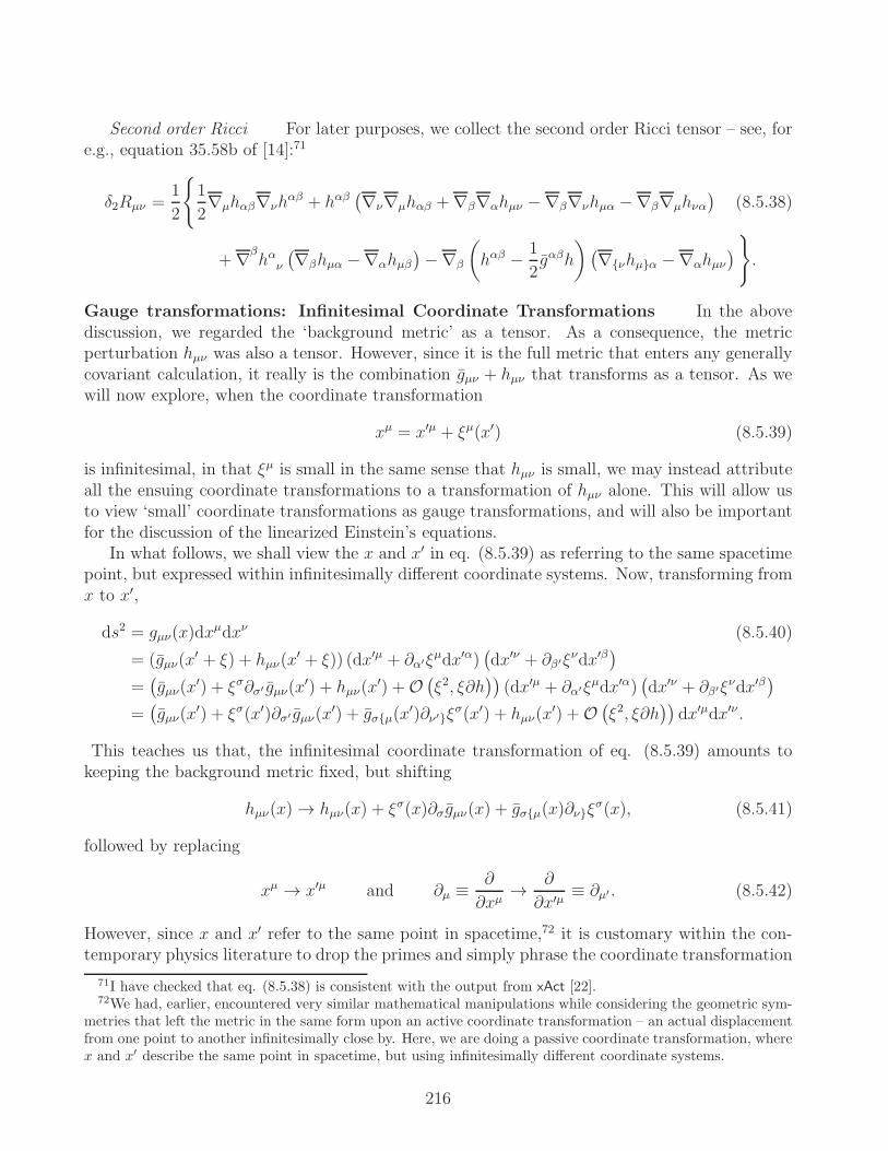
Second order Ricci For later purposes, we collect the second order Ricci tensor – see, fore.g., equation 35.58b of [14]:71

δ2Rµν =1

2

1

2∇µhαβ∇νh

αβ + hαβ(∇ν∇µhαβ +∇β∇αhµν −∇β∇νhµα −∇β∇µhνα

)(8.5.38)

+∇βhαν

(∇βhµα −∇αhµβ

)−∇β

(hαβ − 1

2gαβh

)(∇νhµα −∇αhµν

).

Gauge transformations: Infinitesimal Coordinate Transformations In the abovediscussion, we regarded the ‘background metric’ as a tensor. As a consequence, the metricperturbation hµν was also a tensor. However, since it is the full metric that enters any generallycovariant calculation, it really is the combination gµν + hµν that transforms as a tensor. As wewill now explore, when the coordinate transformation

xµ = x′µ + ξµ(x′) (8.5.39)

is infinitesimal, in that ξµ is small in the same sense that hµν is small, we may instead attributeall the ensuing coordinate transformations to a transformation of hµν alone. This will allow usto view ‘small’ coordinate transformations as gauge transformations, and will also be importantfor the discussion of the linearized Einstein’s equations.

In what follows, we shall view the x and x′ in eq. (8.5.39) as referring to the same spacetimepoint, but expressed within infinitesimally different coordinate systems. Now, transforming fromx to x′,

ds2 = gµν(x)dxµdxν (8.5.40)

= (gµν(x′ + ξ) + hµν(x

′ + ξ)) (dx′µ + ∂α′ξµdx′α)(dx′ν + ∂β′ξνdx′β

)

=(gµν(x

′) + ξσ∂σ′ gµν(x′) + hµν(x

′) +O(ξ2, ξ∂h

))(dx′µ + ∂α′ξµdx′α)

(dx′ν + ∂β′ξνdx′β

)

=(gµν(x

′) + ξσ(x′)∂σ′ gµν(x′) + gσµ(x

′)∂ν′ξσ(x′) + hµν(x

′) +O(ξ2, ξ∂h

))dx′µdx′ν .

This teaches us that, the infinitesimal coordinate transformation of eq. (8.5.39) amounts tokeeping the background metric fixed, but shifting

hµν(x) → hµν(x) + ξσ(x)∂σgµν(x) + gσµ(x)∂νξσ(x), (8.5.41)

followed by replacing

xµ → x′µ and ∂µ ≡ ∂

∂xµ→ ∂

∂x′µ≡ ∂µ′ . (8.5.42)

However, since x and x′ refer to the same point in spacetime,72 it is customary within the con-temporary physics literature to drop the primes and simply phrase the coordinate transformation

71I have checked that eq. (8.5.38) is consistent with the output from xAct [22].72We had, earlier, encountered very similar mathematical manipulations while considering the geometric sym-

metries that left the metric in the same form upon an active coordinate transformation – an actual displacementfrom one point to another infinitesimally close by. Here, we are doing a passive coordinate transformation, wherex and x′ describe the same point in spacetime, but using infinitesimally different coordinate systems.

216

as replacement rules:

xµ → xµ + ξµ(x), (8.5.43)

gµν(x) → gµν(x), (8.5.44)

hµν(x) → hµν(x) +∇µξν(x); (8.5.45)

where we have recognized

ξσ∂σ gµν + gσµ∂νξσ = ∇µξν. (8.5.46)

Problem 8.34. Gauge transformations of a tensor Consider perturbing a spacetimetensor

T µ1...µNν1...νM

≡ Tµ1...µN

ν1...νM+ δT µ1...µN

ν1...νM, (8.5.47)

where δT µ1...µNν1...νM

is small in the same sense that ξα and hµν are small. Perform the infinites-imal coordinate transformation in eq. (8.5.39) on the tensor in eq. (8.5.47) and attribute allthe transformations to the δT µ1...µN

ν1...νM. Write down the ensuing gauge transformation, in di-

rect analogy to eq. (8.5.45). Can you write it in a generally covariant form? Then justify thestatement:

“If the background tensor is zero, the perturbed tensor is gauge-invariant at firstorder in coordinate transformations.”

8.6 Special Topic 2: Conformal/Weyl Transformations

In this section, we collect for the reader’s reference, the conformal transformation propertiesof various geometric objects. We shall define a conformal transformation on a metric to be achange of the geometry by an overall spacetime dependent scale. That is,

gµν(x) ≡ Ω2(x)gµν(x). (8.6.1)

The inverse metric is

gµν(x) = Ω(x)−2gµν(x), gµσgσν ≡ δµν . (8.6.2)

We shall now enumerate how the geometric objects/operations built out of gµν is related to thatbuilt out of gµν . In what follows, all indices on barred tensors are raised and lowered with gµν

and gµν while all indices on un-barred tensors are raised/lowered with gµν and gµν ; the covariantderivative ∇ is with respect to gµν while the ∇ is with respect to gµν .

Metric Determinant Since

det gµν = det(Ω2gµν

)= Ω2d det gµν , (8.6.3)

we must also have

|g|1/2 = Ωd|g|1/2. (8.6.4)

217

Scalar Gradients The scalar gradient with a lower index is just a partial derivative.Therefore

∇µϕ = ∇µϕ = ∂µϕ. (8.6.5)

while ∇µϕ = gµν∇νϕ = Ω−2gµν∇νϕ, so

∇µϕ = Ω−2∇µϕ. (8.6.6)

Scalar Wave Operator The wave operator in the geometry gµν is defined as

≡ gµν∇µ∇ν = ∇µ∇µ. (8.6.7)

By a direct calculation, the wave operator with respect to gµν acting on a scalar ψ is

ϕ =1

Ω2

(d− 2

Ω∇µΩ · ∇µ

ϕ+ϕ

), (8.6.8)

where is the wave operator with respect to gµν . We also have

(Ωsψ) =1

Ω2

(sΩs−1Ω+ s (d+ s− 3)Ωs−2∇µΩ∇

µΩ)ψ

+ (2s+ d− 2)Ωs−1∇µΩ∇µψ + Ωsψ

. (8.6.9)

Scalar Field Action In d dimensional spacetime, the following action involving the scalarϕ and Ricci scalar R[g],

S[ϕ] ≡∫

ddx√

|g|12

(gαβ∇αϕ∇βϕ+

d− 2

4(d− 1)Rϕ2

), (8.6.10)

is invariant – up to surface terms – under the simultaneous replacements

gαβ → Ω2gαβ, gαβ → Ω−2gαβ,√|g| → Ωd

√|g|, (8.6.11)

ϕ→ Ω1− d2ϕ. (8.6.12)

The jargon here is that ϕ transforms covariantly under conformal transformations, with weights = 1 − (d/2). We see in two dimensions, d = 2, a minimally coupled massless scalar theoryautomatically enjoys conformal/Weyl symmetry.Christoffel Symbols A direct calculation shows:

Γµαβ[g] = Γ

µ

αβ[g] +(∂α ln Ω

)δµβ − gαβ g

µν (∂ν lnΩ) (8.6.13)

= Γµ

αβ[g] +(∇α ln Ω

)δµβ − gαβ∇

µln Ω. (8.6.14)

Riemann Tensor By viewing the difference between gµν and gµν as a ‘perturbation’,

gµν − gµν =(Ω2 − 1

)gµν ≡ hµν , (8.6.15)

218

we may employ the results in §(8.5). In particular, eq. (8.5.24) may be used to infer that theRiemann tensor is

Rαβµν [g] = Rα

βµν [g] +∇β∇[µ ln Ωδαν] − gβ[ν∇µ]∇

αln Ω

+ δα[µ∇ν] ln Ω∇β ln Ω +∇αln Ω∇[µ ln Ωgν]β +

(∇ ln Ω

)2gβ[µδ

αν]. (8.6.16)

Ricci Tensor In turn, the Ricci tensor is

Rβν [g] = Rβν [g] + (2− d)∇β∇ν ln Ω− gβν ln Ω (8.6.17)

+ (d− 2)(∇β ln Ω∇ν ln Ω− gβν

(∇ ln Ω

)2). (8.6.18)

Ricci Scalar Contracting the Ricci tensor with gβν = Ω−2gβν, we conclude

R[g] = Ω−2(R[g] + 2(1− d) ln Ω + (d− 2)(1− d)

(∇ ln Ω

)2)(8.6.19)

Weyl Tensor The Weyl tensor, for spacetime dimensions greater than two (d > 2), isdefined to be the completely trace-free portion of the Riemann tensor:

Cµναβ ≡ Rµναβ − 1

d− 2

(Rα[µgν]β − Rβ[µgν]α

)+

gµ[αgβ]ν(d− 2)(d− 1)

R[g]. (8.6.20)

By a direct calculation, one may verify Cµναβ has the same index-symmetries as Rµναβ andis indeed completely traceless: gµαCµναβ = 0. Using equations (8.6.1), (8.6.16), (8.6.17), and(8.6.19), one may then deduce the Weyl tensor with one upper index is invariant under conformaltransformations:

Cµναβ [g] = Cµ

ναβ[g]. (8.6.21)

If we lower the index µ on both sides,

Cµναβ [g] = Ω2Cµναβ [g]. (8.6.22)

Einstein Tensor From equations (8.6.1), (8.6.17) and (8.6.19), we may also compute thetransformation of the Einstein tensor Gβν ≡ Rβν − (gβν/2)R.

Gβν [g] = Gβν [g] + (2− d)(∇β∇ν ln Ω− gβν ln Ω

)

+ (d− 2)

(∇β ln Ω∇ν ln Ω− gβν

3− d

2

(∇ ln Ω

)2)

(8.6.23)

Notice the Einstein tensor is invariant under constant conformal transformations: Gβν [g] =Gβν [g] whenever ∂µΩ = 0.

To reiterate: on the right-hand-sides of these expressions for the Riemann tensor, Ricci tensorand scalar, all indices are raised and lowered with g; for example, (∇A)2 ≡ gστ∇σA∇τA and∇α

A ≡ gαλ∇λA. The Rαβµν [g] is built out of the metric gαβ but the Rα

βµν [g] is built entirelyout of gµν , etc.

219

9 Linear Partial Differential Equations (PDEs)

A partial differential equation (PDE) is a differential equation involving more than one variable.Much of fundamental physics – electromagnetism, quantum mechanics, gravitation and more– involves PDEs. We will first examine Poisson’s equation, and introduce the concept of theGreen’s function, in order to solve it. Because the Laplacian ~∇2 will feature a central role in ourstudy of PDEs, we will study its eigenfunctions/values in various contexts. Then we will usetheir spectra to tackle the heat/diffusion equation via an initial value formulation. In the finalsections we will study the wave equation in flat spacetime, and study various routes to obtainits solutions, both in position/real spacetime and in Fourier space.

9.1 Laplacians and Poisson’s Equation

9.1.1 Poisson’s equation, uniqueness of solutions

Poisson’s equation in D-space is defined to be

−~∇2ψ(~x) = J(~x), (9.1.1)

where J is to be interpreted as some given mass/charge density that sources the Newtonian/electricpotential ψ. The most physically relevant case is in 3D; if we use Cartesian coordinates, Poisson’sequation reads

−~∇2ψ(~x) = −(

∂2ψ

∂(x1)2+

∂2ψ

∂(x2)2+

∂2ψ

∂(x3)2

)= J(~x). (9.1.2)

We will soon see how to solve eq. (9.1.1) by first solving for the inverse of the negative Laplacian(≡ Green’s function).Uniqueness of solution We begin by showing that the solution of Poisson’s equation (eq.(9.1.1)) in some domain D is unique once ψ is specified on the boundary of the domain ∂D. Aswe shall see, this theorem holds even in curved spaces. If it is the normal derivative ni∇iψ thatis specified on the boundary ∂D, then ψ is unique up to an additive constant.

The proof goes by contradiction. Suppose there were two distinct solutions, ψ1 and ψ2. Letus start with the integral

I ≡∫

D

dD~x√

|g|∇iΨ†∇iΨ ≥ 0. (9.1.3)

That this is greater or equal to zero, even in curved spaces, can be seen by writing the gradients

in an orthonormal frame (cf. eq. (7.2.47)), where gij = ε ia ε

j

bδab.73 The

√|g| is always positive,

since it describes volume, whereas ∇iΨ∇iΨ is really a sum of squares.

√|g|δab∇aΨ

†∇bΨ =√

|g|∑

a

|∇aΨ|2 ≥ 0. (9.1.4)

73Expressing the gradients in an orthonormal frame is, in fact, the primary additional ingredient to this proof,when compared to the flat space case. Moreover, notice this proof relies on the Euclidean (positive definite)nature of the metric.

220

We may now integrate-by-parts eq. (9.1.3) and use the curved space Gauss’ theorem in eq.(7.4.35).

I =

∫

∂D

dD−1Σi ·Ψ†∇iΨ−∫

D

dD~x√|g| ·Ψ†∇i∇iΨ. (9.1.5)

Remember from eq. (7.4.26) that dD−1Σi∇iΨ = dD−1~ξ

√|H(~ξ)|ni∇iΨ, where ni is the unit

(outward) normal to the boundary ∂D. If either ψ(∂D) or ni∂iψ(∂D) is specified, therefore, thefirst term on the right hand side of eq. (9.1.5) is zero – since Ψ(∂D) = ψ1(∂D) − ψ2(∂D) andni∂iΨ(∂D) = ni∂iψ1(∂D)− ni∂iψ2(∂D). The seccond term is zero too, since

−∇i∇iΨ = −∇i∇i(ψ1 − ψ2) = J − J = 0. (9.1.6)

But we have just witnessed how I is itself the integral, over the domain, of the sum of squaresof |∇aΨ|. The only way summing squares of something is zero is that something is identicallyzero.

∇aΨ = ε ia ∂iΨ = 0, (everywhere in D). (9.1.7)

Viewing the ε ia as a vector field, so ∇aΨ is the derivative of Ψ in the ath direction, this translates

to the conclusion that Ψ = ψ1−ψ2 is constant in every direction, all the way up to the boundary;i.e., ψ1 and ψ2 can at most differ by an additive constant. If the normal derivative ni∇iψ(∂D)were specified, so that ni∇iΨ = 0 there, then ψ1(~x)−ψ2(~x) = non-zero constant can still yield thesame normal derivative. However, if instead ψ(∂D) were specified on the boundary, Ψ(∂D) = 0there, and must therefore be zero everywhere in D. In other words ψ1 = ψ2, and there cannotbe more than 1 distinct solution. This completes the proof.

9.1.2 (Negative) Laplacian as a Hermitian operator

We will now demonstrate that the negative Laplacian in some domain D can be viewed as aHermitian operator, if its eigenfunctions obey

ψλ(∂D) = 0 (Dirichlet) (9.1.8)

or

ni∇iψλ(∂D) = 0 (Neumann), (9.1.9)

or if there are no boundaries.74 The steps we will take here are very similar to those in the unique-ness proof above. Firstly, by Hermitian we mean the negative Laplacian enjoys the propertythat

I ≡∫

D

dD~x√

|g(~x)|ψ†1(~x)

(−~∇2

~xψ2(~x))=

∫

D

dD~x√

|g(~x)|(−~∇2

~xψ†1(~x)

)ψ2(~x), (9.1.10)

74In this chapter on PDEs we will focus mainly on Dirichlet (and occasionally, Neumann) boundary conditions.There are plenty of other possible boundary conditions, of course.

221

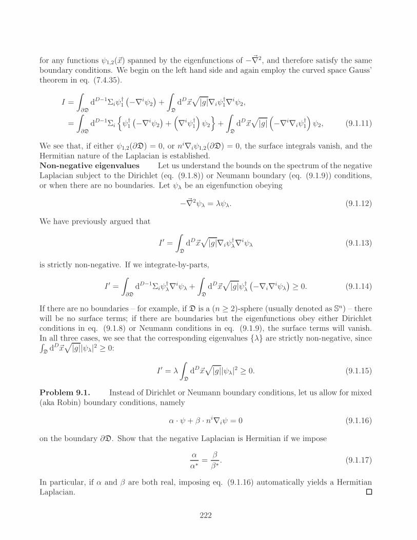
for any functions ψ1,2(~x) spanned by the eigenfunctions of −~∇2, and therefore satisfy the sameboundary conditions. We begin on the left hand side and again employ the curved space Gauss’theorem in eq. (7.4.35).

I =

∫

∂D

dD−1Σiψ†1

(−∇iψ2

)+

∫

D

dD~x√

|g|∇iψ†1∇iψ2,

=

∫

∂D

dD−1Σi

ψ†1

(−∇iψ2

)+(∇iψ†

1

)ψ2

+

∫

D

dD~x√

|g|(−∇i∇iψ

†1

)ψ2, (9.1.11)

We see that, if either ψ1,2(∂D) = 0, or ni∇iψ1,2(∂D) = 0, the surface integrals vanish, and theHermitian nature of the Laplacian is established.Non-negative eigenvalues Let us understand the bounds on the spectrum of the negativeLaplacian subject to the Dirichlet (eq. (9.1.8)) or Neumann boundary (eq. (9.1.9)) conditions,or when there are no boundaries. Let ψλ be an eigenfunction obeying

−~∇2ψλ = λψλ. (9.1.12)

We have previously argued that

I ′ =

∫

D

dD~x√

|g|∇iψ†λ∇iψλ (9.1.13)

is strictly non-negative. If we integrate-by-parts,

I ′ =

∫

∂D

dD−1Σiψ†λ∇iψλ +

∫

D

dD~x√

|g|ψ†λ

(−∇i∇iψλ

)≥ 0. (9.1.14)

If there are no boundaries – for example, if D is a (n ≥ 2)-sphere (usually denoted as Sn) – therewill be no surface terms; if there are boundaries but the eigenfunctions obey either Dirichletconditions in eq. (9.1.8) or Neumann conditions in eq. (9.1.9), the surface terms will vanish.In all three cases, we see that the corresponding eigenvalues λ are strictly non-negative, since∫DdD~x

√|g||ψλ|2 ≥ 0:

I ′ = λ

∫

D

dD~x√|g||ψλ|2 ≥ 0. (9.1.15)

Problem 9.1. Instead of Dirichlet or Neumann boundary conditions, let us allow for mixed(aka Robin) boundary conditions, namely

α · ψ + β · ni∇iψ = 0 (9.1.16)

on the boundary ∂D. Show that the negative Laplacian is Hermitian if we impose

α

α∗=

β

β∗. (9.1.17)

In particular, if α and β are both real, imposing eq. (9.1.16) automatically yields a HermitianLaplacian.

222

9.1.3 Inverse of the negative Laplacian: Green’s function and reciprocity

Given the Dirichlet boundary condition in eq. (9.1.8), i.e., ψλ(∂D) = 0, we will now under-stand how to solve Poisson’s equation, through the inverse of the negative Laplacian. Roughlyspeaking,

−~∇2ψ = J ⇒ ψ =(−~∇2

)−1

J. (9.1.18)

(The actual formula, in a finite domain, will be a tad more complicated, but here we are merelymotivating the reason for defining G.) Since, given any Hermitian operator

H =∑

λ

λ |λ〉 〈λ| , λ ∈ R, (9.1.19)

its inverse is

H−1 =∑

λ

|λ〉 〈λ|λ

, λ ∈ R; (9.1.20)

we see that the inverse of the negative Laplacian in the position space representation is thefollowing mode expansion involving its eigenfunctions ψλ.

G(~x, ~x′) =

⟨~x

∣∣∣∣1

−~∇2

∣∣∣∣ ~x′⟩

=∑

λ

ψλ(~x)ψλ(~x′)†

λ, (9.1.21)

−~∇2ψλ = λψλ, ψλ(~x) ≡ 〈~x| λ〉 . (9.1.22)

(The summation sign is schematic; it can involve either (or both) a discrete sum or/and anintegral over a continuum.) Since the mode functions are subject to ψλ(∂D) = 0, the Green’sfunction itself also obeys Dirichlet boundary conditions:

G(~x ∈ D, ~x′) = G(~x, ~x′ ∈ D) = 0. (9.1.23)

The Green’s function G satisfies the PDE

−~∇2~xG(~x, ~x

′) = −~∇2~x′G(~x, ~x′) =

δ(D)(~x− ~x′)4√

|g(~x)g(~x′))|, (9.1.24)

because the negative Laplacian is Hermitian and thus its eigenfunctions obey the followingcompleteness relation (cf. (4.3.18))

∑

λ

ψλ(~x)†ψλ(~x

′) =δ(D)(~x− ~x′)4√|g(~x)g(~x′))|

. (9.1.25)

Eq. (9.1.24) follows from −~∇2ψλ = λψλ and

−~∇2~xG(~x, ~x

′) =∑

λ

−~∇2~xψλ(~x)ψλ(~x

′)†

λ=∑

λ

ψλ(~x)ψλ(~x′)†, (9.1.26)

−~∇2~x′G(~x, ~x′) =

∑

λ

ψλ(~x)(−~∇2~x′ψλ(~x

′)†)

λ=∑

λ

ψλ(~x)ψλ(~x′)†. (9.1.27)

223

Because the δ(D)-functions on the right hand side of eq. (9.1.24) is the (position representation)of the identity operator, the Green’s function itself is really the inverse of the negative Laplacian.

Physically speaking these δ-functions also lend eq. (9.1.24) to the interpretation that theGreen’s function is the field at ~x produced by a point source at ~x′. Therefore, the Green’sfunction of the negative Laplacian is the gravitational/electric potential produced by a unitstrength point charge/mass.

Isolated zero eigenvalue implies non-existence of inverse Within a finite domainD, we see that the Neumann boundary conditions ni∇iψλ(∂D) = 0 imply there must be azero eigenvalue; for, the ψ0 = constant is the corresponding eigenvector, whose normal derivativeon the boundary is zero:

−~∇2ψ0 = −∂i

(√|g|gij∂jψ0

)

√|g|

= 0 · ψ0. (9.1.28)

As long as this is an isolated zero – i.e., there are no eigenvalues continuously connected to λ = 0– this mode will contribute a discrete term in the mode sum of eq. (9.1.21) that yields a 1/0infinity. That is, the inverse of the Laplacian does not make sense if there is an isolated zeromode.75

Discontinuous first derivatives Because it may not be apparent from the mode ex-pansion in eq. (9.1.21), it is worth highlighting that the Green’s function must contain discon-tinuous first derivatives as ~x → ~x′ in order to yield, from a second order Laplacian, δ-functionson the right hand side of eq. (9.1.24). For Green’s functions in a finite domain D, there arepotentially additional discontinuities when both ~x and ~x′ are near the boundary of the domain∂D.

Flat RD and Method of Images An example is provided by the eigenfunctions of thenegative Laplacian in infinite D-space.

ψ~k(~x) =ei~k·~x

(2π)D/2, −~∇2

~xψ~k(~x) =~k2ψ~k(~x). (9.1.29)

Because we know the integral representation of the δ-function, eq. (9.1.25) now reads

∫

RD

dD~k

(2π)Dei~k·(~x−~x′) = δ(D)(~x− ~x′). (9.1.30)

Through eq. (9.1.21), we may write down the integral representation of the inverse of thenegative Laplacian in Euclidean D-space.

G(~x, ~x′) =

∫

RD

dD~k

(2π)Dei~k·(~x−~x′)

~k2=

Γ(D2− 1)

4πD/2|~x− ~x′|D−2. (9.1.31)

Now, one way to think about the Green’s function GD(D) of the negative Laplacian in a finitedomain D of flat space is to view it as the sum of its counterpart in infinite RD plus a term

75In the infinite flat RD case below, we will see the exp(i~k · ~x) are the eigenfunctions and hence there is also

a zero mode, gotten by setting ~k → ~0. However the inverse does exist because the mode sum of eq. (9.1.21) is

really an integral, and the integration measure dD~k ensures convergence of the integral.

224

that is a homogeneous solution HD(D) in the finite domain D, such that the desired boundaryconditions are achieved on ∂D. Namely,

GD(~x, ~x′;D) =

Γ(D2− 1)

4πD/2|~x− ~x′|D−2+H(~x, ~x′;D),

−~∇2~xGD(~x, ~x

′;D) = −~∇2~x′GD(~x, ~x

′;D) = δ(D) (~x− ~x′) , (Cartesian coordinates)

−~∇2~xHD(~x, ~x

′;D) = −~∇2~x′HD(~x, ~x

′;D) = 0, ~x, ~x′ ∈ D. (9.1.32)

If Dirichlet boundary conditions are desired, we would demand

Γ(D2− 1)

4πD/2|~x− ~x′|D−2+H(~x, ~x′;D) = 0 (9.1.33)

whenever ~x ∈ ∂D or ~x′ ∈ ∂D.The method of images, which you will likely learn about in an electromagnetism course, is a

special case of such a strategy of solving the Green’s function. We will illustrate it through thefollowing example. Suppose we wish to solve the Green’s function in a half-infinite space, i.e.,for xD ≥ 0 only, but let the rest of the x1, . . . , xD−1 run over the real line. We further wantthe boundary condition

GD(xD = 0) = GD(x

′D = 0) = 0. (9.1.34)

The strategy is to notice that the infinite plane that is equidistant between one positive andone negative point mass/charge has zero potential, so if we wish to solve the Green’s function(the potential of the positive unit mass) on the half plane, we place a negative unit mass on theopposite side of the boundary at xD = 0. Since the solution to Poisson’s equation is unique, thesolution for xD ≥ 0 is therefore

GD(~x, ~x′;D) =

Γ(D2− 1)

4πD/2|~x− ~x′|D−2− Γ

(D2− 1)

4πD/2|~ξ|D−2, (9.1.35)

|~ξ| ≡

√√√√D−1∑

j=1

(xj − x′j)2 + (xD + x′D)2, xD, x′D ≥ 0.

Mathematically speaking, when the negative Laplacian is applied to the second term in eq.(9.1.35), it yields

∏D−1j=1 δ(x

j − x′j)δ(xD + x′D), but since xD, x′D ≥ 0, the very last δ-functioncan be set to zero. Hence, the second term is a homogeneous solution when attention is restrictedto xD ≥ 0.

Reciprocity We will also now show that the Green’s function itself is a Hermitianobject, in that

G(~x, ~x′)† = G(~x′, ~x) = G(~x, ~x′). (9.1.36)

The first equality follows from the real positive nature of the eigenvalues, as well as the modeexpansion in eq. (9.1.21)

G(~x, ~x′)∗ =∑

λ

ψλ(~x′)ψλ(~x)

†

λ= G(~x′, ~x). (9.1.37)

225

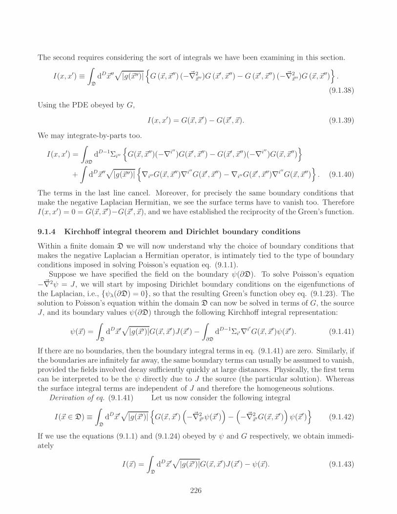
The second requires considering the sort of integrals we have been examining in this section.

I(x, x′) ≡∫

D

dD~x′′√

|g(~x′′)|G (~x, ~x′′) (−~∇2

~x′′)G (~x′, ~x′′)−G (~x′, ~x′′) (−~∇2~x′′)G (~x, ~x′′)

.

(9.1.38)

Using the PDE obeyed by G,

I(x, x′) = G(~x, ~x′)−G(~x′, ~x). (9.1.39)

We may integrate-by-parts too.

I(x, x′) =

∫

∂D

dD−1Σi′′

G(~x, ~x′′)(−∇i′′)G(~x′, ~x′′)−G(~x′, ~x′′)(−∇i′′)G(~x, ~x′′)

+

∫dD~x′′

√|g(~x′′)|

∇i′′G(~x, ~x

′′)∇i′′G(~x′, ~x′′)−∇i′′G(~x′, ~x′′)∇i′′G(~x, ~x′′)

. (9.1.40)

The terms in the last line cancel. Moreover, for precisely the same boundary conditions thatmake the negative Laplacian Hermitian, we see the surface terms have to vanish too. ThereforeI(x, x′) = 0 = G(~x, ~x′)−G(~x′, ~x), and we have established the reciprocity of the Green’s function.

9.1.4 Kirchhoff integral theorem and Dirichlet boundary conditions

Within a finite domain D we will now understand why the choice of boundary conditions thatmakes the negative Laplacian a Hermitian operator, is intimately tied to the type of boundaryconditions imposed in solving Poisson’s equation eq. (9.1.1).

Suppose we have specified the field on the boundary ψ(∂D). To solve Poisson’s equation

−~∇2ψ = J , we will start by imposing Dirichlet boundary conditions on the eigenfunctions ofthe Laplacian, i.e., ψλ(∂D) = 0, so that the resulting Green’s function obey eq. (9.1.23). Thesolution to Poisson’s equation within the domain D can now be solved in terms of G, the sourceJ , and its boundary values ψ(∂D) through the following Kirchhoff integral representation:

ψ(~x) =

∫

D

dD~x′√

|g(~x′)|G(~x, ~x′)J(~x′)−∫

∂D

dD−1Σi′∇i′G(~x, ~x′)ψ(~x′). (9.1.41)

If there are no boundaries, then the boundary integral terms in eq. (9.1.41) are zero. Similarly, ifthe boundaries are infinitely far away, the same boundary terms can usually be assumed to vanish,provided the fields involved decay sufficiently quickly at large distances. Physically, the first termcan be interpreted to be the ψ directly due to J the source (the particular solution). Whereasthe surface integral terms are independent of J and therefore the homogeneous solutions.

Derivation of eq. (9.1.41) Let us now consider the following integral

I(~x ∈ D) ≡∫

D

dD~x′√|g(~x′)|

G(~x, ~x′)

(−~∇2

~x′ψ(~x′))−(−~∇2

~x′G(~x, ~x′))ψ(~x′)

(9.1.42)

If we use the equations (9.1.1) and (9.1.24) obeyed by ψ and G respectively, we obtain immedi-ately

I(~x) =

∫

D

dD~x′√

|g(~x′)|G(~x, ~x′)J(~x′)− ψ(~x). (9.1.43)

226

On the other hand, we may integrate-by-parts,

I(~x) =

∫

∂D

dD−1Σi′

G(~x, ~x′)

(−∇i′ψ(~x′)

)−(−∇i′G(~x, ~x′)

)ψ(~x′)

+

∫

D

dD~x′√

|g(~x′)|∇i′G(~x, ~x

′)∇i′ψ(~x′)−∇i′G(~x, ~x′)∇i′ψ(~x′). (9.1.44)

The second line cancels. Combining equations (9.1.43) and (9.1.44) then hands us the followingKirchhoff representation:

ψ(~x ∈ D) =

∫

∂D

dD−1Σi′

G(~x, ~x′)

(∇i′ψ(~x′)

)−(∇i′G(~x, ~x′)

)ψ(~x′)

+

∫

D

dD~x′√|g(~x′)|G(~x, ~x′)J(~x′). (9.1.45)

76If we recall the Dirichlet boundary conditions obeyed by the Green’s function G(~x, ~x′) (eq.(9.1.23)), the first term on the right hand side of the first line drops out and we obtain eq.(9.1.41).

Problem 9.2. Dirichlet B.C. Variation Principle In a finite domain (where∫DdD~x

√|g| <

∞), let all fields vanish on the boundary ∂D and denote the smallest non-zero eigenvalue of

the negative Laplacian −~∇2 as λ0. Let ψ be an arbitrary function obeying the same boundaryconditions as the eigenfunctions of −~∇2. For this problem, assume that the spectrum of thenegative Laplacian is discrete. Prove that

∫DdD~x

√|g|∇iψ

†∇iψ∫DdD~x

√|g||ψ|2

≥ λ0. (9.1.46)

Just like in quantum mechanics, we have a variational principle for the spectrum of the negativeLaplacian in a finite volume curved space: you can exploit any trial complex function ψ thatvanishes on D to derive an upper bound for the lowest eigenvalue of the negative Laplacian.

Hint: Expand ψ as a superposition of the eigenfunctions of −~∇2. Then integrate-by-partsone of the ∇i in the integrand.

Example Suppose, within a finite 1D box, x ∈ [0, L] we are provided a real field ψ obeying

ψ(x = 0) = α, ψ(x = L) = β (9.1.47)

without any external sources. You can probably solve this 1D Poisson’s equation (−∂2xψ = 0)right away; it is a straight line:

ψ(0 ≤ x ≤ L) = α +β − α

Lx. (9.1.48)

But let us try to solve it using the methods developed here. First, we recall the orthonormaleigenfunctions of the negative Laplacian with Dirichlet boundary conditions,

〈x|n〉 =√

2

Lsin(nπLx), n ∈ 1, 2, 3, . . . ,

∞∑

n=1

〈x|n〉 〈n| x′〉 = δ(x− x′),

−∂2x 〈x|n〉 =(nπL

)2〈x|n〉 . (9.1.49)

76I have put a prime on the index in ∇i′ to indicate the covariant derivative is with respect to ~x′.

227

The mode sum expansion of the Green’s function in eq. (9.1.21) is

G(x, x′) =2

L

∞∑

n=1

(nπL

)−2

sin(nπLx)sin(nπLx′). (9.1.50)

The J term in eq. (9.1.41) is zero, while the surface integrals really only involve evaluation atx = 0, L. Do be careful that the normal derivative refers to the outward normal.

ψ(~x) = ∂x′G(x, x′ = 0)ψ(x′ = 0)− ∂x′G(x, x′ = L)ψ(x′ = L)

= − 2

L

∞∑

n=1

L

nπsin(nπLx) [

cos(nπLx′)ψ(x′)

]x′=L

x′=0

= −∞∑

n=1

2

nπsin(nπLx)((−)n · β − α) (9.1.51)

We may check this answer in the following way. Because the solution in eq. (9.1.51) is odd underx→ −x, let us we extend the solution in the following way:

ψ∞(−L ≤ x ≤ L) = α +β − α

Lx, 0 ≤ x ≤ L,

= −(α +

β − α

Lx

), −L ≤ x < 0. (9.1.52)

We will then extend the definition of ψ∞ by imposing periodic boundary conditions, ψ∞(x+2L) =ψ∞(x). This yields the Fourier series

ψ∞(x) =+∞∑

ℓ=−∞

Cℓei 2πℓ2L

x. (9.1.53)

Multiplying both sides by exp(−i(πn/L)x) and integrating over x ∈ [−L, L].

Cn =

∫ L

−L

ψ∞(x)e−iπnL

x dx

2L=

∫ L

−L

ψ∞(x)(cos(πnLx)− i sin

(πnLx)) dx

2L

= −i∫ L

0

(α +

β − α

Lx

)sin(πnLx) dx

L

=i

πn((−)nβ − α) . (9.1.54)

Putting this back to into the Fourier series,

ψ∞(x) = i

+∞∑

n=1

1

πn

((−)nβ − α) ei

πnL

x −((−)−nβ − α

)e−iπn

Lx

= −+∞∑

n=1

2

πn((−)nβ − α) sin

(πnLx). (9.1.55)

Is it not silly to obtain a complicated infinite sum for a solution, when it is really a straight line?The answer is that, while the Green’s function/mode sum method here does appear unnecessarilycomplicated, this mode expansion method is very general and is oftentimes the only known meansof solving the problem analytically.

228

Problem 9.3. Solve the 2D flat space Poisson equation −(∂2x+∂2y)ψ(0 ≤ x ≤ L1, 0 ≤ y ≤ L2) =

0, up to quadrature, with the following boundary conditions

ψ(0, y) = ϕ1(y), ψ(L1, y) = ϕ2(y), ψ(x, 0) = ρ1(x), ψ(x, L2) = ρ2(x). (9.1.56)

Write the solution as a mode sum, using the eigenfunctions

ψm,n(x, y) ≡ 〈x, y|m,n〉 = 2√L1L2

sin

(πm

L1x

)sin

(πn

L2y

). (9.1.57)

Hint: your answer will involve 1D integrals on the 4 boundaries of the rectangle.

9.2 Laplacians and their spectra

Let us recall our discussions from both linear algebra and differential geometry. Given a (Eu-clidean signature) metric

dℓ2 = gij(~x)dxidxj , (9.2.1)

the Laplacian acting on a scalar ψ can be written as

~∇2ψ ≡ ∇i∇iψ =∂i

(√|g|gij∂jψ

)

√|g|

, (9.2.2)

where√|g| is the square root of the determinant of the metric.

Spectra Now we turn to the primary goal of this section, to study the eigenvector/valueproblem

−~∇2ψλ(~x) = −~∇2 〈~x|λ〉 = λ 〈~x|λ〉 . (9.2.3)

9.2.1 Infinite RD in Cartesian coordinates

In infinite flat Euclidean D-space RD, we have already seen that the plane waves exp(i~k · ~x)are the eigenvectors of −~∇2 with eigenvalues k2|−∞ < k <∞. This is a coordinate invariantstatement, since the ψ and Laplacian in eq. (9.2.3) are coordinate scalars. Also notice that theeigenvalue/vector equation (9.2.3) is a “local” PDE in that it is possible to solve it only in thefinite neighborhood of ~x; it therefore requires appropriate boundary conditions to pin down thecorrect eigen-solutions.

In Cartesian coordinates, moreover,

ψ~k(~x) = ei~k·~x =

D∏

j=1

eikjxj

, ~k2 = δijkikj =D∑

i=1

(ki)2 ≡ ~k2, (9.2.4)

with completeness relations (cf. (4.3.18)) given by∫

RD

dD~x⟨~k∣∣∣ ~x⟩⟨

~x∣∣∣~k′⟩= (2π)Dδ(D)

(~k − ~k′

), (9.2.5)

∫

RD

dD~k

(2π)D

⟨~x∣∣∣~k⟩ ⟨

~k∣∣∣ ~x′⟩= δ(D) (~x− ~x′) . (9.2.6)

229

Translation symmetry and degeneracy For a fixed 1 ≤ i ≤ D, notice the translation operatorin the ith Cartesian direction, namely −i∂j ≡ −i∂/∂xj commutes with −~∇2. The translationoperators commute amongst themselves too. This is why one can simultaneously diagonalizethe Laplacian, and all the D translation operators.

−i∂j 〈~x| k2⟩= kj 〈~x| k2

⟩(9.2.7)

In fact, we see that the eigenvector of the Laplacian |k2〉 can be viewed as a tensor product ofthe eigenstates of Pj .

∣∣∣k2 = ~k2⟩= |k1〉 ⊗ |k2〉 ⊗ · · · ⊗ |kD〉 (9.2.8)

〈~x| k2⟩=(⟨x1∣∣⊗ · · · ⊗

⟨xD∣∣) (|k1〉 ⊗ · · · ⊗ |kD〉)

=⟨x1∣∣ k1⟩ ⟨x2∣∣ k2⟩. . .⟨xD∣∣ kD

⟩=

D∏

j=1

eikjxj

. (9.2.9)

As we have already highlighted in the linear algebra of continuous spaces section, the spectrumof the negative Laplacian admits an infinite fold degeneracy here. Physically speaking we mayassociate it with the translation symmetry of RD.

9.2.2 1 Dimension

Infinite Flat Space In one dimension, the metric77 is

dℓ2 = dz2, (9.2.10)

for z ∈ R, and eq. (9.2.4) reduces to

−~∇21ψk(z) = −∂2zψk(z) = k2ψk(z), 〈z| k〉 ≡ ψk(z) = eikz; (9.2.11)

and their completeness relation (cf. eq. (4.3.18)) is

∫ ∞

−∞

dk

2π〈z| k〉 〈k| z′〉 =

∫ ∞

−∞

dk

2πeik(z−z′) = δ(z − z′). (9.2.12)

Periodic infinite space If the 1D space obeys periodic boundary conditions, with periodL, we have instead

−~∇21ψm(z) = −∂2zψm(z) =

(2πm

L

)2

ψm(z),

〈z|m〉 ≡ ψm(z) = L−1/2ei2πmL

z, m = 0,±1,±2, . . . . (9.2.13)

The orthonormal eigenvectors obey

∫ L

0

dz 〈m| z〉 〈z|m′〉 = δmm′ , 〈z|m〉 = L−1/2ei2πmL

z; (9.2.14)

77One dimensional space(time)s are always flat – the Riemann tensor is identically zero.

230

while their completeness relation reads, for 0 ≤ z, z′ ≤ L,

∞∑

m=−∞

〈z|m〉 〈m| z′〉 = 1

L

∞∑

m=−∞

e2πmL

i(z−z′) = δ(z − z′). (9.2.15)

Unit Circle A periodic infinite space can be thought of as a circle, and vice versa. Simplyidentify L ≡ 2πr, where r is the radius of the circle as embedded in 2D space. For concretenesswe will consider a circle of radius 1. Then we may write the metric as

dℓ2 = (dφ)2, φ ∈ [0, 2π). (9.2.16)

We may then bring over the results from the previous discussion.

−~∇2S1ψm(φ) = −∂2φψm(φ) = m2ψm(φ),

〈φ|m〉 ≡ ψm(φ) = (2π)−1/2eimφ, m = 0,±1,±2, . . . . (9.2.17)

The orthonormal eigenvectors obey

∫ 2π

0

dφ 〈m| φ〉 〈φ|m′〉 = δmm′ , 〈φ|m〉 = (2π)−1/2eimφ. (9.2.18)

while their completeness relation reads, for 0 ≤ z, z′ ≤ L,

∞∑

m=−∞

〈φ|m〉 〈m| φ′〉 = 1

2π

∞∑

m=−∞

eim(φ−φ′) = δ(φ− φ′). (9.2.19)

Fourier series re-visited. Note that −i∂φ can be thought of as the “momentum opera-tor” on the unit circle (in the position representation) with eigenvalues m and correspondingeigenvectors 〈φ|m〉. Namely, if we define

〈φ |Pφ|ψ〉 = −i∂φ 〈φ|ψ〉 (9.2.20)

for any state |ψ〉, we shall see it is Hermitian. Given arbitrary states |ψ1,2〉,

〈ψ1 |Pφ|ψ2〉 =∫ 2π

0

dφ 〈ψ1| φ〉 (−i∂φ 〈φ|ψ2〉) (9.2.21)

= [−i 〈ψ1|φ〉 〈φ|ψ2〉]φ=2πφ=0 +

∫ 2π

0

dφ (i∂φ 〈ψ1|φ〉) 〈φ|ψ2〉 .

As long as we are dealing with the space of continuous functions ψ1,2(φ) on a circle, the boundaryterms must vanish because φ = 0 and φ = 2π really refer to the same point. Therefore,

〈ψ1 |Pφ|ψ2〉 =∫ 2π

0

dφ (−i∂φ 〈φ|ψ1〉)∗ 〈φ|ψ2〉 =∫ 2π

0

dφ〈φ |Pφ|ψ1〉 〈φ|ψ2〉

=

∫ 2π

0

dφ⟨ψ1

∣∣∣P †φ

∣∣∣φ⟩〈φ|ψ2〉 =

⟨ψ1

∣∣∣P †φ

∣∣∣ψ2

⟩. (9.2.22)

231

We must therefore have

⟨φ∣∣e−iθPφ

∣∣ψ⟩= e−iθ(−i∂φ) 〈φ|ψ〉 = e−θ∂φ 〈φ|ψ〉 = 〈φ− θ|ψ〉 . (9.2.23)

Any function on a circle can be expanded in the eigenstates of Pφ, which in turn can be expressedthrough its position representation.

|ψ〉 =+∞∑

ℓ=−∞

|m〉 〈m|ψ〉 =+∞∑

ℓ=−∞

∫ 2π

0

dφ |φ〉 〈φ|m〉 〈m|ψ〉 =+∞∑

ℓ=−∞

∫ 2π

0

dφ√2π

|φ〉 〈m|ψ〉 eimφ,

〈m|ψ〉 =∫ 2π

0

dφ′ 〈m| φ′〉 〈φ′|ψ〉 =∫ 2π

0

dφ′

√2πe−imφ′

ψ(φ′). (9.2.24)

This is nothing but the Fourier series expansion of ψ(φ).

9.2.3 2 Dimensions

Flat Space, Cylindrical Coordinates The 2D flat metric in cylindrical coordinates reads

dℓ2 = dr2 + r2dφ2, r ≥ 0, φ ∈ [0, 2π),√|g| = r. (9.2.25)

The negative Laplacian is therefore

−~∇22ϕk(r, φ) = −1

r

(∂r (r∂rϕk) +

1

r∂2φϕk

)(9.2.26)

= −1

r∂r (r∂rϕk) +

1

r2∂2φϕk

. (9.2.27)

Our goal here is to diagonalize the negative Laplacian in cylindrical coordinates, and re-writethe plane wave using its eigenstates. In this case we will in fact tackle the latter and use theresults to do the former. To begin, note that the plane wave in 2D cylindrical coordinates is

〈~x|~k〉 = exp(i~k · ~x) = exp(ikr cos(φ− φk)), k ≡ |~k|, r ≡ |~x|; (9.2.28)

because the Cartesian components of ~k and ~x are

ki = k (cosφk, sinφk) xi = r (cos φ, sinφ) . (9.2.29)

We observe that this is a periodic function of the angle ∆φ ≡ φ− φk with period L = 2π, whichmeans it must admit a Fourier series expansion. Referring to equations (4.5.114) and (4.5.115),

〈~x|~k〉 =+∞∑

m=−∞

χm(kr)eim(φ−φk)

√2π

. (9.2.30)

and

χm(kr) =

∫ 2π

0

dφ′′

√2πeikr cosφ

′′e−imφ′′

(9.2.31)

232

=√2π

∫ φ′′=2π

φ′′=0

d(φ′′ + π/2)

2πeikr cos(φ

′′+π/2−π/2)e−im(φ′′+π/2−π/2)

=√2π

∫ 5π/2

π/2

dφ′

2πeikr sinφ′

e−imφ′im = im

√2π

∫ +π

−π

dφ′

2πeikr sinφ′

e−imφ′

(In the last line, we have used the fact that the integrand is itself a periodic function of φ′ withperiod 2π to change the limits of integration.) As it turns out, the Bessel function Jm admitsan integral representation (cf. eq. (10.9.2) of the NIST page here.)

Jm(z) =

∫ π

−π

dφ′

2πeiz sinφ′−imφ′

, m ∈ 0,±1,±2, . . . , (9.2.32)

J−m(z) = (−)mJm(z). (9.2.33)

As an aside, Jν(z) also has a series representation

Jν(z) =(z2

)ν ∞∑

k=0

(−)k(z/2)2k

k!Γ(ν + k + 1); (9.2.34)

and the large argument asymptotic expansion

J±ν(z ≫ ν) ∼√

2

πzcos(z ∓ π

2ν − π

4

). (9.2.35)

We have arrived at the result

〈~x|~k〉 = exp(i~k · ~x) = exp(ikr cos(φ− φk)), k ≡ |~k|, r ≡ |~x|

=∞∑

ℓ=−∞

iℓJℓ(kr)eim(φ−φk). (9.2.36)

Because the eimφ are basis vectors on the circle of fixed radius r, every term in the infinite sum

is a linearly independent eigenvector of −~∇22. That is, we can now read off the basis eigenvectors

of the negative Laplacian in 2D cylindrical coordinates. To obtain orthonormal ones, however, letus calculate their normalization using the following orthogonality relation, written in cylindricalcoordinates,

(2π)2δ(k − k′)δ(φk − φk′)√

kk′=

∫

R2

d2x exp(i(~k − ~k′) · ~x) (9.2.37)

=

+∞∑

m,m′=−∞

∫ ∞

0

dr · r∫ 2π

0

dφ · im(−i)m′Jm(kr)Jm′(k′r)eim(φ−φk)e−im′(φ−φk′ )

= (2π)

+∞∑

m=−∞

∫ ∞

0

dr · rJm(kr)Jm(k′r)eim(φk′−φk).

We now replace the δ(φ−φk) on the left hand side with the completeness relation in eq. (9.2.15),where now z = φk, z

′ = φk′ and the period is L = 2π. Equating the result to the last line then

233

brings us to

+∞∑

m=−∞

δ(k − k′)√kk′

eim(φk−φk′) =+∞∑

m=−∞

∫ ∞

0

dr · rJm(kr)Jm(k′r)eim(φk′−φk). (9.2.38)

The coefficients of each (linearly independent) vector eim(φk−φk′ ) on both sides should be thesame. This yields the completeness relation of the radial mode functions:

∫ ∞

0

dr · rJm(kr)Jm(k′r) =δ(k − k′)√

kk′, (9.2.39)

∫ ∞

0

dk · kJm(kr)Jm(kr′) =δ(r − r′)√

rr′. (9.2.40)

To summarize, we have found, in 2D infinite flat space, that the eigenvectors/values of thenegative Laplacian in cylindrical coordinates (r ≥ 0, 0 ≤ φ < 2π) are

−~∇22 〈r, φ| k,m〉 = k2 〈r, φ| k,m〉 , 〈r, φ| k,m〉 ≡ Jm(kr)

exp (imφ)√2π

,

m = 0,±1,±2,±3, . . . . (9.2.41)

The eigenvectors are normalized as∫ ∞

0

dr · r∫ 2π

0

dφ 〈k,m| r, φ〉 〈r, φ| k′, m′〉 = δmm′δ(k − k′)√

kk′. (9.2.42)

Rotational symmetry and degeneracy Note that −i∂φ is the translation operator in theazimuthal direction (≡ rotation operator), with eigenvalue m. The spectrum here is discretelyand infinitely degenerate, which can be physically interpreted to be due to the presence ofrotational symmetry.

Bessel’s equation As a check of our analysis here, we may now directly evaluate the2D negative Laplacian acting on the its eigenvector 〈r, φ| k,m〉, and see that we are lead toBessel’s equation. Starting from the eigenvector/value equation in (9.2.41), followed by usingthe explicit expression in eq. (9.2.26) and the angular eigenvalue/vector equation ∂2φ exp(imφ) =−m2 exp(imφ), this hands us

k2Jm(kr) = −1

r∂r (r∂rJm(kr))−

m2

r2Jm(kr)

. (9.2.43)

Let us then re-scale ρ ≡ kr, where k ≡ |~k|, so that ∂r = k∂ρ.

ρ2 · J ′′(ρ) + ρ · J ′(ρ) + (ρ2 −m2)J(ρ) = 0 (9.2.44)

Equation 10.2.1 of the NIST page here tells us we have indeed arrived at Bessel’s equation. Twolinearly independent solutions are Jm(kr) and Ym(kr). However, eq. (10.2.2) of the NIST pagehere and eq. (10.8.1) of the NIST page here tell us, for small argument, Ym(z → 0) has at leasta log singularity of the form ln(z/2) and for m 6= 0 has also a power law singularity that goesas 1/z|m|. Whereas, Jm(z) is (z/2)

|m| times a power series in the variable (z/2)2, and is not onlysmooth for small z, the power series in fact has an infinite radius of convergence. It makes sensethat our plane wave expansion only contains Jm and not Ym because it is smooth for all r.

234

Problem 9.4. Explain how you would modify the analysis here, if we were not dealingwith an infinite 2D space, but only a wedge of 2D space – namely, r ≥ 0 but 0 ≤ φ ≤ φ0 < 2π.How would you modify the analysis here, if φ ∈ [0, 2π), but now 0 ≤ r ≤ r0 < ∞? You do notneed to carry out the calculations in full, but try to be as detailed as you can. Assume Dirichletboundary conditions.

2-sphere S2, Separation-Of-Variables, and the Spherical Harmonics78 The 2-sphereof radius R can be viewed as a curved surface embedded in 3D flat space parametrized as

~x(~ξ = (θ, φ)) = R (sin θ cosφ, sin θ sin φ, cos θ) , ~x2 = R2. (9.2.45)

For concreteness we will consider the case where R = 1. Its metric is therefore given by HIJ =∂Ix

i∂JxjdξIdξJ,

HIJdξIdξJ = dθ2 + (sin θ)2dφ2,

√|H| = sin θ. (9.2.46)

(Or, simply take the 3D flat space metric in spherical coordinates, and set dr → 0 and r → 1.)We wish to diagonalize the negative Laplacian on this unit radius 2−sphere. The relevant

eigenvector/value equation is

−~∇2S2Y (θ, φ) = ν(ν + 1)Y (θ, φ), (9.2.47)

where ν for now is some arbitrary positive number.To do so, we now turn to the separation of variables technique, which is a method to reduce a

PDE into a bunch of ODEs – and hence more manageable. The main idea is, for highly symmetricproblems such as the Laplacian in flat space(time)s or on the D-sphere, one postulates that amulti-variable eigenfunction factorizes into a product of functions, each depending only on onevariable. If solutions can be found, then we are assured that such an ansatz works.

In the unit radius 2−sphere case we postulate

Y (θ, φ) = Λ(θ)Φ(φ). (9.2.48)

First work out the Laplacian explicitly, with s ≡ sin θ,

−1

s∂θ (s∂θY ) +

1

s2∂2φY

= −

1

s∂θ (s∂θY ) +

1

s2~∇2

S1Y

= ν(ν + 1)Y (θ, φ). (9.2.49)

We have identified ~∇2S1

= ∂2φ to be the Laplacian on the circle, from eq. (9.2.17). This suggests

we should choose Φ to be the eigenvector of ~∇2S1.

Φ(φ) ∝ exp(imφ), m = 0,±1,±2, . . . (9.2.50)

Moreover, it will turn out to be very useful to change variables to c ≡ cos θ, which runs from −1to +1 over the range 0 ≤ θ ≤ π. Since s ≡ sin θ is strictly positive there, we have the positiveroot sθ = (1− c2)1/2 and ∂θ = (∂c/∂θ)∂c = − sin θ∂c = −(1− c2)1/2∂c.

−−∂c

(−(1− c2)∂cΛ · Φ

)+

1

1− c2Λ · ∂2φΦ

= ν(ν + 1)Λ · Φ

78In these notes we focus solely on the spherical harmonics on S2; for spherical harmonics in arbitrary dimen-sions, see arXiv:1205.3548.

235

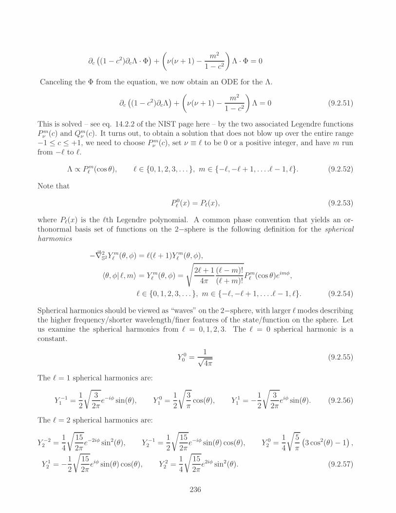
∂c((1− c2)∂cΛ · Φ

)+

(ν(ν + 1)− m2

1− c2

)Λ · Φ = 0

Canceling the Φ from the equation, we now obtain an ODE for the Λ.

∂c((1− c2)∂cΛ

)+

(ν(ν + 1)− m2

1− c2

)Λ = 0 (9.2.51)

This is solved – see eq. 14.2.2 of the NIST page here – by the two associated Legendre functionsPmν (c) and Qm

ν (c). It turns out, to obtain a solution that does not blow up over the entire range−1 ≤ c ≤ +1, we need to choose Pm

ν (c), set ν ≡ ℓ to be 0 or a positive integer, and have m runfrom −ℓ to ℓ.

Λ ∝ Pmℓ (cos θ), ℓ ∈ 0, 1, 2, 3, . . ., m ∈ −ℓ,−ℓ+ 1, . . . .ℓ− 1, ℓ. (9.2.52)

Note that

P 0ℓ (x) = Pℓ(x), (9.2.53)

where Pℓ(x) is the ℓth Legendre polynomial. A common phase convention that yields an or-thonormal basis set of functions on the 2−sphere is the following definition for the sphericalharmonics

−~∇2S2Y

mℓ (θ, φ) = ℓ(ℓ+ 1)Y m

ℓ (θ, φ),

〈θ, φ| ℓ,m〉 = Y mℓ (θ, φ) =

√2ℓ+ 1

4π

(ℓ−m)!

(ℓ+m)!Pmℓ (cos θ)eimφ,

ℓ ∈ 0, 1, 2, 3, . . ., m ∈ −ℓ,−ℓ+ 1, . . . .ℓ− 1, ℓ. (9.2.54)

Spherical harmonics should be viewed as “waves” on the 2−sphere, with larger ℓmodes describingthe higher frequency/shorter wavelength/finer features of the state/function on the sphere. Letus examine the spherical harmonics from ℓ = 0, 1, 2, 3. The ℓ = 0 spherical harmonic is aconstant.

Y 00 =

1√4π

(9.2.55)

The ℓ = 1 spherical harmonics are:

Y −11 =

1

2

√3

2πe−iφ sin(θ), Y 0

1 =1

2

√3

πcos(θ), Y 1

1 = −1

2

√3

2πeiφ sin(θ). (9.2.56)

The ℓ = 2 spherical harmonics are:

Y −22 =

1

4

√15

2πe−2iφ sin2(θ), Y −1

2 =1

2

√15

2πe−iφ sin(θ) cos(θ), Y 0

2 =1

4

√5

π

(3 cos2(θ)− 1

),

Y 12 = −1

2

√15

2πeiφ sin(θ) cos(θ), Y 2

2 =1

4

√15

2πe2iφ sin2(θ). (9.2.57)

236

The ℓ = 3 spherical harmonics are:

Y −33 =

1

8

√35

πe−3iφ sin3(θ), Y −2

3 =1

4

√105

2πe−2iφ sin2(θ) cos(θ),

Y −13 =

1

8

√21

πe−iφ sin(θ)

(5 cos2(θ)− 1

), Y 0

3 =1

4

√7

π

(5 cos3(θ)− 3 cos(θ)

),

Y 13 = −1

8

√21

πeiφ sin(θ)

(5 cos2(θ)− 1

), Y 2

3 =1

4

√105

2πe2iφ sin2(θ) cos(θ),

Y 33 = −1

8

√35

πe3iφ sin3(θ). (9.2.58)

For later purposes, note that the m = 0 case removes any dependence on the azimuthal angleφ, and in fact returns the Legendre polynomial.

〈θ, φ| ℓ,m = 0〉 = Y 0ℓ (θ, φ) =

√2ℓ+ 1

4πPℓ(cos θ). (9.2.59)

Orthonormality and completeness of the spherical harmonics read, respectively,

〈ℓ′, m′| ℓ,m〉 =∫

S2d2~ξ√

|H| Y m′ℓ′ (θ, φ)Y m

ℓ (θ, φ)

=

∫ +1

−1

d(cos θ)

∫ 2π

0

dφY m′ℓ′ (θ, φ)Y m

ℓ (θ, φ) = δℓ′ℓ δ

m′m , (9.2.60)

and

〈θ′, φ′| θ, φ〉 = δ(θ′ − θ)δ(φ− φ′)√sin(θ) sin(θ′)

= δ (cos(θ′)− cos(θ)) δ(φ− φ′)

=

∞∑

ℓ=0

ℓ∑

m=−ℓ

Y mℓ (θ′, φ′)Y m

ℓ (θ, φ). (9.2.61)

In 3D flat space, let us write the Cartesian components of the momentum vector ~k and theposition vector ~x in spherical coordinates.

ki = k (sin θk · cosφk, sin θk · sinφk, cos θk) ≡ kk (9.2.62)

xi = r (sin θ · cosφ, sin θ · sinφ, cos θ) ≡ rx (9.2.63)

Addition formula In terms of these variables we may write down a useful identity involvingthe spherical harmonics and the Legendre polynomial, usually known as the addition formula.

Pℓ

(k · x

)=

4π

2ℓ+ 1

+ℓ∑

m=−ℓ

Y mℓ (θ, φ)Y m

ℓ (θk, φk) =4π

2ℓ+ 1

+ℓ∑

m=−ℓ

Y mℓ (θ, φ)Y m

ℓ (θk, φk), (9.2.64)

where k ≡ ~k/k and x ≡ ~x/r. The second equality follows from the first because the Legendrepolynomial is real.

237

For a fixed direction k, note that Pℓ(k · x) in eq. (9.2.64) is an eigenvector of the negative

Laplacian on the 2−sphere. For, as we have already noted, the eigenvalue equation −~∇2ψ = λψis a coordinate scalar. In particular, we may choose coordinates such that k is pointing ‘North’,so that k · x = cos θ, where θ is the usual altitude angle. By recalling eq. (9.2.59), we seetherefore,

−~∇2~x,S2Pℓ

(k · x

)= ℓ(ℓ+ 1)Pℓ

(k · x

). (9.2.65)

Since Pℓ(k ·x) is symmetric under the swap k ↔ x, it must also be an eigenvector of the Laplacian

with respect to ~k,

−~∇2~k,S2

Pℓ

(k · x

)= ℓ(ℓ+ 1)Pℓ

(k · x

). (9.2.66)

Complex conjugation Under complex conjugation, the spherical harmonics obey

Y mℓ (θ, φ) = (−)mY −m

ℓ (θ, φ). (9.2.67)

Parity Under a parity flip, meaning if you compare Y mℓ evaluated at the point (θ, φ) to the

point on the opposite side of the sphere (π − θ, φ+ π), we have the relation

Y mℓ (π − θ, φ+ π) = (−)ℓY m

ℓ (θ, φ). (9.2.68)

The odd ℓ spherical harmonics are thus odd under parity; whereas the even ℓ ones are invariant(i.e., even) under parity.Poisson Equation on the 2-sphere Having acquired some familiarity of the spherical har-monics, we can now tackle Poisson’s equation

−~∇2S2ψ(θ, φ) = J(θ, φ) (9.2.69)

on the 2−sphere. Because the spherical harmonics are complete on the sphere, we may expandboth ψ and J in terms of them.

ψ =∑

ℓ,m

Amℓ Y

mℓ , J =

∑

ℓ,m

Bmℓ Y

mℓ . (9.2.70)

(This means, if J is a given function, then we may calculate Bmℓ =

∫S2d2ΩY m

ℓ (θ, φ)J(θ, φ).)

Inserting these expansions into eq. (9.2.69), and recalling the eigenvalue equation −~∇2S2Y mℓ =

ℓ(ℓ+ 1)Y mℓ ,

∑

ℓ 6=0,m

ℓ(ℓ+ 1)Amℓ Y

mℓ =

∑

ℓ,m

Bmℓ Y

mℓ . (9.2.71)

On the left hand side, because the eigenvalue of Y 00 is zero, there is no longer any ℓ = 0 term.

Therefore, we see that for there to be a consistent solution, J itself cannot contain a ℓ = 0 term.

238

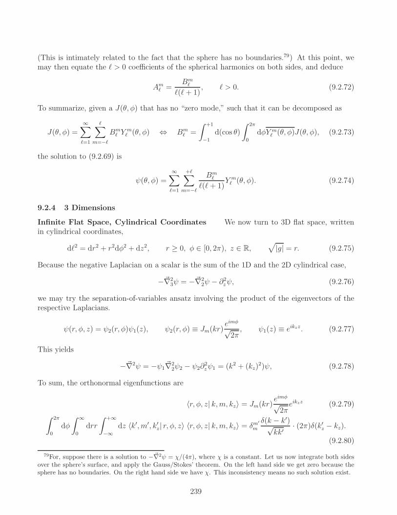
(This is intimately related to the fact that the sphere has no boundaries.79) At this point, wemay then equate the ℓ > 0 coefficients of the spherical harmonics on both sides, and deduce

Amℓ =

Bmℓ

ℓ(ℓ+ 1), ℓ > 0. (9.2.72)

To summarize, given a J(θ, φ) that has no “zero mode,” such that it can be decomposed as

J(θ, φ) =∞∑

ℓ=1

ℓ∑

m=−ℓ

Bmℓ Y

mℓ (θ, φ) ⇔ Bm

ℓ =

∫ +1

−1

d(cos θ)

∫ 2π

0

dφY mℓ (θ, φ)J(θ, φ), (9.2.73)

the solution to (9.2.69) is

ψ(θ, φ) =

∞∑

ℓ=1

+ℓ∑

m=−ℓ

Bmℓ

ℓ(ℓ+ 1)Y mℓ (θ, φ). (9.2.74)

9.2.4 3 Dimensions

Infinite Flat Space, Cylindrical Coordinates We now turn to 3D flat space, writtenin cylindrical coordinates,

dℓ2 = dr2 + r2dφ2 + dz2, r ≥ 0, φ ∈ [0, 2π), z ∈ R,√

|g| = r. (9.2.75)

Because the negative Laplacian on a scalar is the sum of the 1D and the 2D cylindrical case,

−~∇23ψ = −~∇2

2ψ − ∂2zψ, (9.2.76)

we may try the separation-of-variables ansatz involving the product of the eigenvectors of therespective Laplacians.

ψ(r, φ, z) = ψ2(r, φ)ψ1(z), ψ2(r, φ) ≡ Jm(kr)eimφ

√2π, ψ1(z) ≡ eikzz. (9.2.77)

This yields

−~∇2ψ = −ψ1~∇2

2ψ2 − ψ2∂2zψ1 = (k2 + (kz)

2)ψ, (9.2.78)

To sum, the orthonormal eigenfunctions are

〈r, φ, z| k,m, kz〉 = Jm(kr)eimφ

√2πeikzz (9.2.79)

∫ 2π

0

dφ

∫ ∞

0

drr

∫ +∞

−∞

dz 〈k′, m′, k′z| r, φ, z〉 〈r, φ, z| k,m, kz〉 = δm′

m

δ(k − k′)√kk′

· (2π)δ(k′z − kz).

(9.2.80)

79For, suppose there is a solution to −~∇2ψ = χ/(4π), where χ is a constant. Let us now integrate both sidesover the sphere’s surface, and apply the Gauss/Stokes’ theorem. On the left hand side we get zero because thesphere has no boundaries. On the right hand side we have χ. This inconsistency means no such solution exist.

239

Since we already figured out the 2D plane wave expansion in cylindrical coordinates in eq.(9.2.36), and since the 3D plane wave is simply the 2D one multiplied by the plane wave in the z

direction, i.e., exp(i~k ·~x) = exp(ikr cos(φ−φk)) exp(ikzz), we may write down the 3D expansionimmediately

〈~x|~k〉 = exp(i~k · ~x) =∞∑

ℓ=−∞

iℓJℓ(kr)eim(φ−φk)eikzz, (9.2.81)

where

ki = (k cosφk, k sinφk, kz) , xi = (r cos φ, r sin φ, z) . (9.2.82)

Infinite Flat Space, Spherical Coordinates We now turn to 3D flat space written inspherical coordinates,

dℓ2 = dr2 + r2dΩ2S2 , dΩ2

S2 ≡ dθ2 + (sin θ)2dφ2,

r ≥ 0, φ ∈ [0, 2π), θ ∈ [0, π],√

|g| = r2 sin θ. (9.2.83)

The Laplacian on a scalar is

~∇2ψ =1

r2∂r(r2∂rψ

)+

1

r2~∇2

S2ψ. (9.2.84)

where ~∇2S2

is the Laplacian on a 2−sphere.Plane wave With

ki = k (sin(θk) cos(φk), sin(θk) sin(φk), cos(θk)) ≡ kk, (9.2.85)

xi = r (sin(θ) cos(φ), sin(θ) sin(φ), cos(θ)) ≡ rx, (9.2.86)

we have

〈~x|~k〉 = exp(i~k · ~x) = exp(ikrk · x

). (9.2.87)

If we view k as the 3−direction, this means the plane wave has no dependence on the azimuthalangle describing rotation about the 3−direction. This in turn indicates we should be able toexpand 〈~x|~k〉 using Pℓ(k · ~x).

exp(ikrk · x

)=

∞∑

ℓ=0

χℓ(kr)

√2ℓ+ 1

4πPℓ

(k · x

). (9.2.88)

For convenience we have used the Y 0ℓ in eq. (9.2.59)) as our basis. Exploiting the orthonormality

of the spherical harmonics to solve for the expansion coefficients:

χℓ(kr) = 2π

∫ +1

−1

dceikrcY 0ℓ (θ, φ) =

√(4π)(2ℓ+ 1)

1

2

∫ +1

−1

dceikrcPℓ(c). (9.2.89)

240

(Even though the integral is over the entire solid angle, the azimuthal integral is trivial andyields 2π immediately.) At this point we may refer to eq. (10.54.2) of the NIST page here forthe following integral representation of the spherical Bessel function of integer order,

iℓjℓ(z) =1

2

∫ +1

−1

dceizcPℓ(c), ℓ = 0, 1, 2, . . . . (9.2.90)

(The spherical Bessel function jℓ(z) is real when z is positive.) We have arrived at

〈~x|~k〉 = exp(i~k · ~x) =∞∑

ℓ=0

(2ℓ+ 1)iℓjℓ(kr)Pℓ

(k · x

), k ≡ |~k| (9.2.91)

= 4π

∞∑

ℓ=0

iℓjℓ(kr)

+ℓ∑

m=−ℓ

Y mℓ (θ, φ)Y m

ℓ (θk, φk), (9.2.92)

where, for the second equality, we have employed the additional formula in eq. (9.2.64).Spectrum Just as we did for the 2D plane wave, we may now read off the eigenfunctions ofthe 3D flat Laplacian in spherical coordinates. First we compute the normalization.

∫

R3

d3~x exp(i(~k − ~k′) · ~x) = (2π)3δ(k − k′)

kk′δ (cos(θk′)− cos(θk)) δ (φk − φk′) (9.2.93)

Switching to spherical coordinates within the integral on the left-hand-side,

(4π)2∫

S2d2Ω

∫ ∞

0

drr2∞∑

ℓ,ℓ′=0

iℓ(−i)ℓ′jℓ(kr)jℓ′(k′r)

×+ℓ∑

m=−ℓ

+ℓ′∑

m′=−ℓ′

Y mℓ (θ, φ)Y m

ℓ (θk, φk)Ym′ℓ′ (θk, φk)Y m′

ℓ′ (θ, φ)

= (4π)2∫ ∞

0

drr2∞∑

ℓ=0

jℓ(kr)jℓ(k′r)

+ℓ∑

m=−ℓ

Y mℓ (θ, φ)Y m

ℓ (θ, φ). (9.2.94)

Comparing the right hand sides of the two preceding equations, and utilizing the completenessrelation obeyed by the spherical harmonics,

4(2π)2∫ ∞

0

drr2∞∑

ℓ=0

jℓ(kr)jℓ(k′r)

+ℓ∑

m=−ℓ

Y mℓ (θk, φk)Y m

ℓ (θk, φk)

= (2π)3δ(k − k′)

kk′

∞∑

ℓ=0

+ℓ∑

m=−ℓ

Y mℓ (θk, φk)Y

mℓ (θk, φk). (9.2.95)

Therefore it must be that∫ ∞

0

drr2jℓ(kr)jℓ(k′r) =

π

2

δ(k − k′)

kk′. (9.2.96)

241

Referring to eq. (10.47.3) of the NIST page here,

jℓ(z) =

√π

2zJℓ+ 1

2(z) (9.2.97)

we see this is in fact the same result as in eq. (9.2.39).To sum, we have diagonalized the 3D flat space negative Laplacian in spherical coordinates

as follows.

−~∇2 〈r, θ, φ| k, ℓ,m〉 = k2 〈r, θ, φ| k, ℓ,m〉 ,

〈r, θ, φ| k, ℓ,m〉 =√

2

πjℓ(kr)Y

mℓ (θ, φ), (9.2.98)

〈k′, ℓ′, m′| k, ℓ,m〉 =∫

S2d2Ω

∫ ∞

0

drr2 〈k′, ℓ′, m′| r, θ, φ〉 〈r, θ, φ| k, ℓ,m〉 ,

=δ(k − k′)

kk′δℓ

′ℓ δ

m′m .

Problem 9.5. Prolate Ellipsoidal Coordinates in 3D Flat Space 3D Euclidean spacecan be foliated by prolate ellipsoids in the following way. Let ~x ≡ (x1, x2, x3) be Cartesiancoordinates; ρ be the size of a given prolate ellipsoid; and the angular coordinates (0 ≤ θ ≤π, 0 ≤ φ < 2π) specify a point on its 2D surface. Then,

~x =(√

ρ2 −R2 sin θ cos φ,√ρ2 −R2 sin θ sinφ, ρ cos θ

); (9.2.99)

ρ ≥ R, (θ, φ) ∈ S2. (9.2.100)

Explain the geometric meaning of the constant R. Work out the 3D flat metric in prolateellipsoidal coordinates (ρ, θ, φ) and proceed to diagonalize the associated scalar Laplacian ~∇2 ≡gij∇i∇j. Hint: The spherical harmonics Y m

ℓ (θ, φ) will turn out to still be very useful here.

9.3 Heat/Diffusion Equation

9.3.1 Definition, uniqueness of solutions

We will define the heat or diffusion equation to be the PDE

∂tψ (t, ~x) = σ~∇2~xψ (t, ~x) =

σ√|g|∂i

(√|g|gij∂jψ

), σ > 0, (9.3.1)

where ~∇2~x is the Laplacian with respect to some metric gij(~x), which we will assume does not

depend on the time t. We will also assume the ψ(t, ~x) is specified on the boundary of the domaindescribed by gij(~x), i.e., it obeys Dirichlet boundary conditions.

The diffusion constant σ has dimensions of length if ~∇2 is of dimensions 1/[Length2]. Wemay set σ = 1 and thereby describe all other lengths in the problem in units of σ. As the heatequation, this PDE describes the temperature distribution as a function of space and time. Asthe diffusion equation in flat space, it describes the probability density of finding a point particleundergoing (random) Brownian motion. As we shall witness, the solution of eq. (9.3.1) is aidedby the knowledge of the eigenfunctions/values of the Laplacian in question.

242

Uniqueness of solution Suppose the following initial conditions are given

ψ(t = t0, ~x) = ϕ0(~x), (9.3.2)

and suppose the field ψ or its normal derivative is specified on the boundaries ∂D,

ψ(t, ~x ∈ ∂D) = ϕ3(∂D), (Dirichlet), (9.3.3)

or ni∇iψ(t, ~x ∈ ∂D) = ϕ4(∂D), (Neumann), (9.3.4)

where ni(∂D) is the unit outward normal vector. Then, the solution to the heat/diffusionequation in eq. (9.3.1) is unique.

Proof Without loss of generality, since our heat/diffusion equation is linear, we may assumethe field is real. We then suppose there are two such solutions ψ1 and ψ2; the proof is establishedif we can show, in fact, that ψ1 has to be equal to ψ2. Note that the difference Ψ ≡ ψ1 − ψ2 issubject to the initial conditions

Ψ(t = t0, ~x) = 0, (9.3.5)

and the spatial boundary conditions

Ψ(t, ~x ∈ ∂D) = 0 or ni∇iΨ(t, ~x ∈ ∂D) = 0. (9.3.6)

Let us then consider the following (non-negative) integral

ρ(t) ≡ 1

2

∫

D

dD~x√

|g(~x)|Ψ(t, ~x)2 ≥ 0, (9.3.7)

as well as its time derivative

∂tρ(t) =

∫

D

dD~x√

|g(~x)|ΨΨ. (9.3.8)

We may use the heat/diffusion equation on the Ψ term, and integrate-by-parts one of the gra-dients on the second term,

∂tρ(t) =

∫

D

dD~x√|g(~x)|Ψ~∇2Ψ

=

∫

∂D

dD−1~ξ

√|H(~ξ)|Ψni∇iΨ−

∫

D

dD~x√

|g(~x)|∇iΨ∇iΨ. (9.3.9)

By assumption either Ψ or ni∇iΨ is zero on the spatial boundary; therefore the first term onthe second line is zero. We have previously argued that the integrand in the second term on thesecond line is strictly non-negative

∇iΨ∇iΨ =∑

i

(∇iΨ)2 ≥ 0. (9.3.10)

This implies

∂tρ(t) = −∫

D

dD~x√

|g(~x)|∇iΨ∇iΨ ≤ 0. (9.3.11)

However, the initial conditions Ψ(t = t0, ~x) = 0 indicate ρ(t = t0) = 0 (cf. eq. (9.3.7)).Moreover, since ρ(t ≥ t0) has to be non-negative from its very definition and since we have justshown its time derivative is non-positive, ρ(t ≥ t0) therefore has to remain zero for all subsequenttime t ≥ t0; i.e., it cannot decrease below zero. And because ρ(t) is the integral of the square ofΨ, the only way it can be zero is Ψ = 0 ⇒ ψ1 = ψ2. This establishes the theorem.

243

9.3.2 Heat Kernel, Solutions with ψ(∂D) = 0

In this section we introduce the propagator, otherwise known as the heat kernel, which will proveto be key to solving the heat/diffusion equation. It is the matrix element

K(~x, ~x′; s ≥ 0) ≡⟨~x∣∣∣es~∇2

∣∣∣ ~x′⟩. (9.3.12)

It obeys the heat/diffusion equation

∂sK(~x, ~x′; s) =⟨~x∣∣∣~∇2es

~∇2∣∣∣ ~x′⟩=⟨~x∣∣∣es~∇2 ~∇2

∣∣∣ ~x′⟩

= ~∇2~xK(~x, ~x′; s) = ~∇2

~x′K(~x, ~x′; s), (9.3.13)

where we have assumed ~∇2 is Hermitian. K also obeys the initial condition

K(~x, ~x′; s = 0) = 〈~x| ~x′〉 = δ(D)(~x− ~x′)4√g(~x)g(~x′)

. (9.3.14)

If we demand the eigenfunctions of ~∇2 obey Dirichlet boundary conditions,ψλ(∂D) = 0

∣∣∣−~∇2ψλ = λψλ

, (9.3.15)

then the heat kernel obeys the same boundary conditions.

K(~x ∈ ∂D, ~x′; s) = K(~x, ~x′ ∈ ∂D; s) = 0. (9.3.16)

To see this we need to perform a mode expansion. By inserting in eq. (9.3.14) a complete set of

the eigenstates of ~∇2, the heat kernel has an explicit solution

K(~x, ~x′; s ≥ 0) =⟨~x∣∣∣es~∇2

∣∣∣ ~x′⟩=∑

λ

e−sλ 〈~x|λ〉 〈λ|~x′〉 , (9.3.17)

where the sum is schematic: depending on the setup at hand, it can consist of either a sum overdiscrete eigenvalues and/or an integral over a continuum. In this form, it is manifest the heatkernel vanishes when either ~x or ~x′ lies on the boundary ∂D.

Initial value problem In this section we will focus on solving the initial value problemwhen the field is itself is zero on the boundary ∂D for all relevant times. This will in fact bethe case for infinite domains; for example, flat RD, whose heat kernel we will work out explicitlybelow. The setup is thus as follows:

ψ(t = t′, ~x) ≡ 〈~x|ψ(t′)〉 (given), ψ(t ≥ t′, ~x ∈ D) = 0. (9.3.18)

Then ψ(t, ~x) at any later time t > t′ is given by

ψ(t ≥ t′, ~x) =⟨~x∣∣∣e(t−t′)~∇2

∣∣∣ψ(t′)⟩=

∫dD~x′

√|g(~x′)|

⟨~x∣∣∣e(t−t′)~∇2

∣∣∣ ~x′⟩〈~x′|ψ(t′)〉

=

∫dD~x′

√|g(~x′)|K(~x, ~x′; t− t′)ψ(t′, ~x′). (9.3.19)

244

That this is the correct solution is because the right hand side obeys the heat/diffusion equationthrough eq. (9.3.13). As t → t′, we also see from eq. (9.3.14) that the initial condition isrecovered.

ψ(t = t′, ~x) = 〈~x|ψ(t′)〉 =∫

dD~x′√

|g(~x′)| δ(D)(~x− ~x′)

4√|g(~x′)g(~x)|

ψ(t′, ~x′) = ψ(t′, ~x). (9.3.20)

Moreover, since the heat kernel obeys eq. (9.3.16), the solution automatically maintains theψ(t ≥ t′, ~x ∈ D) = 0 boundary condition.Decay times, Asymptotics Suppose we begin with some temperature distribution T (t′, ~x).By expanding it in the eigenfunctions of the Laplacian, let us observe that it is the componentalong the eigenfunction with the small eigenvalue that dominates the late time temperaturedistribution. From eq. (9.3.19) and (9.3.17),

T (t ≥ t′, ~x) =∑

λ

∫dD~x′

√|g(~x′)|

⟨~x∣∣∣e(t−t′)~∇2

∣∣∣λ⟩〈λ| ~x′〉 〈~x′|T (t′)〉

=∑

λ

e−(t−t′)λ 〈~x|λ〉∫

dD~x′√|g(~x′)| 〈λ|~x′〉 〈~x′|T (t′)〉

=∑

λ

e−(t−t′)λ 〈~x|λ〉 〈λ|T (t′)〉 . (9.3.21)

Remember we have proven that the eigenvalues of the Laplacian are strictly non-positive. Thatmeans, as (t− t′) → ∞, the dominant temperature distribution is

T (t− t′ → ∞, ~x) ≈ e−(t−t′)λmin 〈~x|λmin〉∫

dD~x′√

|g(~x′)| 〈λmin| ~x′〉 〈~x′|T (t′)〉 , (9.3.22)

because all the λ > λmin become exponentially suppressed (relative to the λmin state) due to thepresence of e−(t−t′)λ. As long as the minimum eigenvalue λmin is strictly positive, we see the finaltemperature is zero.

T (t− t′ → ∞, ~x) = 0, if λmin > 0. (9.3.23)

When the minimum eigenvalue is zero, we have

T (t− t′ → ∞, ~x) → 〈~x| λ = 0〉∫

dD~x′√

|g(~x′)| 〈λ = 0| ~x′〉 〈~x′|T (t′)〉 , if λmin = 0.

(9.3.24)

The exception to the dominant behavior in eq. (9.3.22) is when there is zero overlap betweenthe initial distribution and that eigenfunction with the smallest eigenvalue, i.e., if

∫dD~x′

√|g(~x′)| 〈λmin| ~x′〉 〈~x′|T (t′)〉 = 0. (9.3.25)

Generically, we may say that, with the passage of time, the component of the initial distributionalong the eigenfunction corresponding to the eigenvalue λ decays as 1/λ; i.e., when t− t′ = 1/λ,its amplitude falls by 1/e.

245

Static limit Another way of phrasing the (t − t′) → ∞ behavior is that – since everyterm in the sum-over-eigenvalues that depends on time decays exponentially, it must be that thelate time asymptotic limit is simply the static limit, when the time derivative on the left handside of eq. (9.3.1) is zero and we obtain Laplace’s equation

0 = ~∇2ψ(t→ ∞, ~x). (9.3.26)

Probability interpretation in flat infinite space In the context of the diffusion equationin flat space, because of the δ-functions on the right hand side of eq. (9.3.14), the propagatorK(~x, ~x′; t − t′) itself can be viewed as the probability density (≡ probability per volume) offinding the Brownian particle – which was infinitely localized at ~x′ at the initial time t′ – at agiven location ~x some later time t > t′. To support this probability interpretation it has to bethat ∫

RD

dD~xK(~x, ~x′; t− t′) = 1. (9.3.27)

The integral on the left hand side corresponds to summing the probability of finding the Brownianparticle over all space – that has to be unity, since the particle has to be somewhere. We canverify this directly, by inserting a complete set of states.

∫

RD

dD~x⟨~x∣∣∣e(t−t′)~∇2

∣∣∣ ~x′⟩=

∫

RD

dD~k

∫

RD

dD~x⟨~x∣∣∣e(t−t′)~∇2

∣∣∣~k⟩ ⟨

~k∣∣∣ ~x′⟩

=

∫

RD

dD~k

∫

RD

dD~xe−(t−t′)~k2〈~x|~k〉⟨~k∣∣∣ ~x′⟩

=

∫

RD

dD~k

∫

RD

dD~xe−(t−t′)~k2 ei~k·(~x−~x′)

(2π)D

=

∫

RD

dD~ke−(t−t′)~k2e−i~k·~x′δ(D)(~k) = 1. (9.3.28)

Heat Kernel in flat space In fact, the same technique allow us to obtain the heat kernelin flat RD.

⟨~x∣∣∣e(t−t′)~∇2

∣∣∣ ~x′⟩=

∫

RD

dD~k⟨~x∣∣∣e(t−t′)~∇2

∣∣∣~k⟩ ⟨

~k∣∣∣ ~x′⟩

(9.3.29)

=

∫

RD

dD~k

(2π)De−(t−t′)~k2ei

~k·(~x−~x′) =

D∏

j=1

∫ +∞

−∞

dkj2π

e−(t−t′)(kj)2eikj(xj−x′j).

We may “complete the square” in the exponent by considering

−(t− t′)

(kj − i

xj − x′j

2(t− t′)

)2

= −(t− t′)

((kj)

2 − ikjxj − x′j

t− t′−(xj − x′j

2(t− t′)

)2). (9.3.30)

The heat kernel in flat RD is therefore⟨~x∣∣∣e(t−t′)σ~∇2

∣∣∣ ~x′⟩= (4πσ(t− t′))

−D/2exp

(− (~x− ~x′)2

4σ(t− t′)

), t > t′, (9.3.31)

where we have put back the diffusion constant σ. If you have taken quantum mechanics, youmay recognize this result to be very similar to the path integral H 〈~x, t|~x′, t′〉H of a free particle.

246

9.3.3 Green’s functions and initial value formulation in a finite domain

Green’s function from Heat Kernel Given the heat kernel defined with Dirichlet bound-ary conditions, the associated Green’s function is defined as

G(t− t′; ~x, ~x′) ≡ Θ(t− t′)K(~x, ~x′; t− t′), (9.3.32)

where we define Θ(s) = 1 for s ≥ 0 and Θ(s) = 0 for s < 0. This Green’s function G obeys

(∂t − ~∇2

~x

)G(t− t′; ~x, ~x′) =

(∂t − ~∇2

~x′

)G(t− t′; ~x, ~x′) = δ(t− t′)

δ(D)(~x− ~x′)4√g(~x)g(~x′)

, (9.3.33)

the boundary condition

G(τ ; ~x ∈ ∂D, ~x′) = G(τ ; ~x, ~x′ ∈ ∂D) = 0, (9.3.34)

as well as the causality condition

G(τ ; ~x, ~x′) = 0 when τ < 0. (9.3.35)

The boundary condition in eq. (9.3.34) follows directly from eq. (9.3.16); whereas eq. (9.3.33)follow from a direct calculation

(∂t − ~∇2

)G(t− t′; ~x, ~x′) = δ(t− t′)K(~x, ~x′; t− t′) + Θ(t− t′)

(∂t − ~∇2

)K(~x, ~x′; t− t′)

= δ(t− t′)δ(D)(~x− ~x′)4√g(~x)g(~x′)

. (9.3.36)

Initial value problem Within a spatial domain D, suppose the initial fieldconfiguration ψ(t′, ~x ∈ D) is given and suppose its value on the spatial boundary ∂Dis also provided (i.e., Dirichlet B.C.’s ψ(t ≥ t′, ~x ∈ ∂D) are specified). The uniquesolution ψ(t ≥ t′, ~x ∈ D) to the heat/diffusion equation (9.3.1) is

ψ(t ≥ t′, ~x) =

∫

D

dD~x′√

|g(~x′)|G(t− t′; ~x, ~x′)ψ(t′, ~x′) (9.3.37)

−∫ t

t′dt′′∫

∂D

dD−1~ξ

√|H(~ξ)|ni′∇i′G

(t− t′′; ~x, ~x′(~ξ)

)ψ(t′′, ~x′(~ξ)

),

where the Green’s function G obeys the PDE in eq. (9.3.33) and the boundaryconditions in equations (9.3.34) and (9.3.35).

Derivation of eq. (9.3.37) We begin by multiplying both sides of eq. (9.3.33) by ψ(t′′, ~x′)and integrating over both space and time (from t′ to infinity).

ψ(t ≥ t′, ~x) =

∫ ∞

t′dt′′∫

D

dD~x′√

|g(~x′)|(∂t − ~∇2

~x′

)G(t− t′′; ~x, ~x′)ψ(t′′, ~x′) (9.3.38)

=

∫ ∞

t′dt′′∫

D

dD~x′√

|g(~x′)|(−∂t′′Gψ +∇i′G∇i′ψ

)

247

−∫ ∞

t′dt′′∫

∂D

dD−1~ξ

√|H(~ξ)|ni′∇i′Gψ

=

∫

D

dD~x′√

|g(~x′)|[−Gψ]t′′=∞

t′′=t′ +

∫ ∞

t′dt′′G

(∂t′′ − ~∇2

~x′′

)ψ

+

∫ ∞

t′dt′′∫

∂D

dD−1~ξ

√|H(~ξ)|

(G · ni′∇i′ψ − ni′∇i′G · ψ

).

If we impose the boundary condition in eq. (9.3.35), we see that [−Gψ]t′′=∞t′′=t′ = G(t − t′)ψ(t′)

because the upper limit contains G(t − ∞) ≡ limt′→−∞Θ(t − t′)K(~x, ~x′; t − t′) = 0. Theheat/diffusion eq. (9.3.1) removes the time-integral term on the first line of the last equality. IfDirichlet boundary conditions were chosen, we may choose G(t − t′′; ~x, ~x′ ∈ ∂D) = 0 (i.e., eq.(9.3.34)) and obtain eq. (9.3.37). Note that the upper limit of integration in the last line isreally t, because eq. (9.3.35) tells us the Green’s function vanishes for t′′ > t.

9.3.4 Problems

Problem 9.6. In infinite flat RD, suppose we have some initial probability distribution offinding a Brownian particle, expressed in Cartesian coordinates as

ψ(t = t0, ~x) =(ωπ

)D/2

exp(−ω(~x− ~x0)

2), ω > 0. (9.3.39)

Solve the diffusion equation for t ≥ t0.

Problem 9.7. Suppose we have some initial temperature distribution T (t = t0, θ, φ) ≡T0(θ, φ) on a thin spherical shell. This distribution admits some multipole expansion:

T0(θ, φ) =

∞∑

ℓ=0

ℓ∑

m=−ℓ

amℓ Ymℓ (θ, φ), amℓ ∈ C. (9.3.40)

The temperature as a function of time obeys the heat/diffusion equation

∂tT (t, θ, φ) = σ~∇2T (t, θ, φ), σ > 0, (9.3.41)

where ~∇2 is now the Laplacian on the 2−sphere. Since ~∇2 is dimensionless here, σ has units of1/[Time].

1. Solve the propagator K for the heat/diffusion equation on the 2−sphere, in terms of aspherical harmonic Y m

ℓ (θ, φ) expansion.

2. Find the solution for T (t > t0, θ, φ).

3. What is the decay rate of the ℓth multipole, i.e., how much time does the ℓth term in themultipole sum take to decay in amplitude by 1/e? Does it depend on both ℓ and m? And,what is the final equilibrium temperature distribution?

248

Problem 9.8. Inverse of Laplacian from Heat Kernel In this problem we want to point outhow the Green’s function of the Laplacian is related to the heat/diffusion equation. To re-cap,the Green’s function itself obeys the D-dimensional PDE:

−~∇2G(~x, ~x′) =δ(D)(~x− ~x′)4√g(~x)g(~x′)

. (9.3.42)

As already suggested by our previous discussions, the Green’s function G(~x, ~x′) can be viewed

the matrix element of the operator G ≡ 1/(−~∇2), namely80

G(~x, ~x′) =⟨~x∣∣∣G∣∣∣ ~x′⟩≡⟨~x

∣∣∣∣1

−~∇2

∣∣∣∣ ~x′⟩. (9.3.43)

The ~∇2 is now an abstract operator acting on the Hilbert space spanned by the position eigenkets|~x〉. Because it is Hermitian, we have

−~∇2~x

⟨~x

∣∣∣∣1

−~∇2

∣∣∣∣ ~x′⟩

=

⟨~x

∣∣∣∣∣−~∇2

−~∇2

∣∣∣∣∣ ~x′

⟩= 〈~x| ~x′〉 = δ(D)(~x− ~x′). (9.3.44)

Now use the Gamma function identity, for Re(z), Re(b) > 0,

1

bz=

1

Γ(z)

∫ ∞

0

tz−1e−btdt, (9.3.45)

where Γ(z) is the Gamma function – to justify

G(~x, ~x′) =

∫ ∞

0

dtKG (~x, ~x′; t) , (9.3.46)

KG (~x, ~x′; t) ≡⟨~x∣∣∣et~∇2

∣∣∣ ~x′⟩.

Notice how the integrand itself is the propagator (eq. (9.3.12)) of the heat/diffusion equation.

We will borrow from our previous linear algebra discussion that −~∇2 = ~P 2, as can be seenfrom its position space representation. Now proceed to re-write this integral by inserting to boththe left and to the right of the operator et

~∇2the completeness relation in momentum space. Use

the fact that ~P 2 = −~∇2 and eq. to deduce

G(~x, ~x′) =

∫ ∞

0

dt

∫dD~k

(2π)De−t~k2ei

~k·(~x−~x′). (9.3.47)

(Going to momentum space allows you to also justify in what sense the restriction Re(b) > 0of the formula in eq. (9.3.45) was satisfied.) By appropriately “completing the square” in theexponent, followed by an application of eq. (9.3.45), evaluate this integral to arrive at theGreen’s function of the Laplacian in D spatial dimensions:

G(~x, ~x′) =

⟨~x

∣∣∣∣1

−~∇2

∣∣∣∣ ~x′⟩

=Γ(D2− 1)

4πD/2|~x− ~x′|D−2, (9.3.48)

80The perspective that the Green’s function be viewed as an operator acting on some Hilbert space wasadvocated by theoretical physicist Julian Schwinger.

249

where |~x− ~x′| is the Euclidean distance between ~x and ~x′.Next, can you use eq. 18.12.4 of the NIST page here to perform an expansion of the Green’s

function of the negative Laplacian in terms of r> ≡ max(r, r′), r< ≡ min(r, r′) and n · n′, wherer ≡ |~x|, r′ ≡ |~x′|, n ≡ ~x/r, and n′ ≡ ~x′/r′? The D = 3 case reads

1

4π|~x− ~x′| = (4πr>)−1

∞∑

ℓ=0

Pℓ (n · n′)

(r<r>

)ℓ

=1

r>

∞∑

ℓ=0

ℓ∑

m=−ℓ

Y mℓ (n)Y m

ℓ (n′)

2ℓ+ 1

(r<r>

)ℓ

, (9.3.49)

where the Pℓ are Legendre polynomials and in the second line the addition formula of eq. (9.2.64)was invoked.

Note that while it is not easy to verify by direct differentiation that eq. (9.3.48) is indeed

the Green’s function 1/(−~∇2), one can do so by performing the integral over t in eq. (9.3.47),to obtain

G(~x, ~x′) =

∫dDk

(2π)Dei~k·(~x−~x′)

~k2. (9.3.50)

We have already seen this in eq. (9.1.31).Finally, can you use the relationship between the heat kernel and the Green’s function of the

Laplacian in eq. (9.3.46), to show how in a finite domain, eq. (9.3.37) leads to eq. (9.1.41) inthe late time t→ ∞ limit? (You may assume the smallest eigenvalue of the negative Laplacianis strictly positive; recall eq. (9.1.46).)

Problem 9.9. Is it possible to solve for the Green’s function of the Laplacian on the 2-sphere? Use the methods of the last two problems, or simply try to write down the mode sumexpansion in eq. (9.1.21), to show that you would obtain a 1/0 infinity. What is the reason forthis apparent pathology? Suppose we could solve

−~∇2G(~x, ~x′) =δ(2)(~x− ~x′)4√g(~x)g(~x′)

. (9.3.51)

Perform a volume integral of both sides over the 2−sphere – explain the contradiction you get.(Recall the discussion in the differential geometry section.) Hint: Apply the curved space Gauss’law in eq. (7.4.35) and remember the 2-sphere is a closed surface.

9.4 Massless Scalar Wave Equation (Mostly) In Flat Spacetime RD,1

9.4.1 Spacetime metric, uniqueness of Minkowski wave solutions

Spacetime Metric In Cartesian coordinates (t, ~x), it is possible associate a metric to flatspacetime as follows

ds2 = c2dt2 − d~x · d~x ≡ ηµνdxµdxν , xµ ≡ (ct, xi), (9.4.1)

250

where c is the speed of light in vacuum; µ ∈ 0, 1, 2, . . . , D; and D is still the dimension ofspace.81 We also have defined the flat (Minkowski) spacetime metric

ηµν ≡ diag (1,−1,−1, . . . ,−1) . (9.4.2)

The generalization of eq. (9.4.1) to curved spacetime is

ds2 = gµν(t, ~x)dxµdxν , xµ = (ct, xi). (9.4.3)

It is common to use the symbol , especially in curved spacetime, to denote the spacetime-Laplacian:

ψ ≡ ∇µ∇µψ =1√|g|∂µ

(√|g|gµν∂νψ

), (9.4.4)

where√

|g| is now the square root of the absolute value of the determinant of the metric gµν .

In Minkowski spacetime of eq. (9.4.1), we have√|g| = 1, ηµν = ηµν , and

ψ = ηµν∂µ∂νψ ≡ ∂2ψ =(c−2∂2t − δij∂i∂j

)ψ; (9.4.5)

where δij∂i∂j = ~∇2 is the spatial Laplacian in flat Euclidean space. The Minkowski “dotproduct” between vectors u and v in Cartesian coordinates is now

u · v ≡ ηµνuµvν = u0v0 − ~u · ~v, u2 ≡ (u0)2 − ~u2, etc. (9.4.6)

From here on, x, x′ and k, etc. – without an arrow over them – denotes collectively the D + 1coordinates of spacetime. Indices of spacetime tensors are moved with gµν and gµν . For instance,

uµ = gµνuν , uµ = gµνuν . (9.4.7)

In the flat spacetime geometry of eq. (9.4.1), written in Cartesian coordinates,

u0 = u0, ui = −ui. (9.4.8)

Indefinite signature The subtlety with the metric of spacetime, as opposed to that of spaceonly, is that the “time” part of the distance in eq. (9.4.1) comes with a different sign fromthe “space” part of the metric. In curved or flat space, if ~x and ~x′ have zero geodesic distancebetween them, they are really the same point. In curved or flat spacetime, however, x and x′

may have zero geodesic distance between them, but they could either refer to the same spacetimepoint (aka “event”) – or they could simply be lying on each other’s light cone:

0 = (x− x′)2 = ηµν(xµ − x′µ)(xν − x′ν) ⇒ (t− t′)2 = (~x− ~x′)2. (9.4.9)

To understand this statement more systematically, let us work out the geodesic distance betweenany pair of spacetime points in flat spacetime.

81In this section it is important to distinguish Greek µ, ν, . . . and Latin/English alphabets a, b, i, j, . . ..The former run over 0 through D, where the 0th index refers to time and the 1st through Dth to space. The latterrun from 1 through D, and are thus strictly “spatial” indices. Also, be aware that the opposite sign convention,ds2 = −dt2 +d~x · d~x, is commonly used too. For most physical applications both sign conventions are valid; see,however, [15].

251

Problem 9.10. In Minkowski spacetime expressed in Cartesian coordinates, the Christoffelsymbols are zero. Therefore the geodesic equation in (7.3.31) returns the following “acceleration-is-zero” ODE:

0 =d2Zµ(λ)

dλ2. (9.4.10)

Show that the geodesic joining the initial spacetime point Zµ(λ = 0) = x′µ to the final locationZµ(λ = 1) = xµ is the straight line

Zµ(0 ≤ λ ≤ 1) = x′µ + λ (xµ − x′µ). (9.4.11)

Use eq. (7.1.22) to show that half the square of the geodesic distance between x′ and x is

σ(x, x′) =1

2(x− x′)2. (9.4.12)

σ is commonly called Synge’s world function in the gravitation literature.

Some jargon needs to be introduced here. (Drawing a spacetime diagram would help.)

• When σ > 0, we say x and x′ are timelike separated. If you sit at rest in some inertialframe, then the tangent vector to your world line is uµ = (1,~0), and u = ∂t is a measureof how fast the time on your watch is running. Or, simply think about setting d~x = 0 inthe Minkowski metric: ds2 → dt2 > 0.

• When σ < 0, we say x and x′ are spacelike separated. If you and your friend sit at rest inthe same inertial frame, then at a fixed time dt = 0, the (square of the) spatial distancebetween the both of you is now given by integrating ds2 → −d~x2 < 0 between your twolocations.

• When σ = 0, we say x and x′ are null (or light-like) separated. As already alluded to, in4 dimensional flat spacetime, light travels strictly on null geodesics ds2 = 0. Consider acoordinate system for spacetime centered at x′; then we would say x lies on the light coneof x′ (and vice versa).

As we will soon discover, the indefinite metric of spacetimes – as opposed to the positive definiteone of space itself – is what allows for wave solutions, for packets of energy/momentum to travelover space and time. In Minkowski spacetime, we will show below, by solving explicitly theGreen’s function GD+1 of the wave operator, that these waves ψ, subject to eq. (9.4.16), willobey causality: they travel strictly on and/or within the light cone, independent of what thesource J is.

Poincare symmetry Analogous to how rotations Ria|δijRi

aRjb = δab and spatial

translations ai leave the flat Euclidean metric δij invariant,

xi → Rijx

j + ai ⇒ δijdxidxj → δijdx

idxj . (9.4.13)

(The Rij and a

i are constants.) Lorentz transformations Λαµ|ηαβΛα

µΛβν = ηµν and spacetime

translations aµ are ones that leave the flat Minkowski metric ηµν invariant.

xα → Λαµx

µ + aα ⇒ ηµνdxµdxν → ηµνdx

µdxν . (9.4.14)

252

(The Λαµ and aα are constants.) This in turn leaves the light cone condition ds2 = 0 invariant

– the speed of light is unity, |d~x|/dt = 1, in all inertial frames related via eq. (9.4.14).Wave Equation In Curved Spacetime The wave equation (for a minimally coupledmassless scalar) in some spacetime geometry gµνdx

µdxν is a 2nd order in time PDE that takesthe following form:

∇µ∇µψ =1√|g|∂µ

(√|g|gµν∂νψ

)= J(x), (9.4.15)

where J is some specified external source of ψ.Minkowski We will mainly deal with the case of infinite flat (aka “Minkowski”) spacetime

in eq. (9.4.1), where in Cartesian coordinates xµ = (ct, ~x). This leads us to the wave equation

(∂2t − c2~∇2

~x

)ψ(t, ~x) = c2J(t, ~x), ~∇2

~x ≡ δij∂i∂j . (9.4.16)

Here, c will turn out to be the speed of propagation of the waves themselves. Because it will bethe most important speed in this chapter, I will set it to unity, c = 1.82 We will work mainlyin flat infinite spacetime, which means the ~∇2 is the Laplacian in flat space. This equationdescribes a diverse range of phenomenon, from the vibrations of strings to that of spacetimeitself.

2D Minkowski We begin the study of the homogeneous wave equation in 2 dimensions.In Cartesian coordinates (t, z),

(∂2t − ∂2z

)ψ(t, z) = 0. (9.4.17)

We see that the solutions are a superposition of either left-moving ψ(z+t) or right-moving wavesψ(z − t), where ψ can be any arbitrary function,

(∂2t − ∂2z

)ψ(z ± t) = (±)2ψ′′(z ± t)− ψ′′(z ± t) = 0. (9.4.18)

Remark It is worth highlighting the difference between the nature of the general solutionsto 2nd order linear homogeneous ODEs versus those of PDEs such as the wave equation here. Inthe former, they span a 2 dimensional vector space, whereas the wave equation admits arbitraryfunctions as general solutions. This is why the study of PDEs involve infinite dimensional(oftentimes continuous) Hilbert spaces.

Let us put back the speed c – by dimensional analysis we know [c]=[Length/Time], so x± ctwould yield the correct dimensions.

ψ(t, x) = ψL(x+ ct) + ψR(x− ct). (9.4.19)

These waves move strictly at speed c.

82This is always a good labor-saving strategy when you solve problems. Understand all the distinct dimensionfulquantities in your setup – pick the most relevant/important length, time, and mass, etc. Then set them to one, soyou don’t have to carry their symbols around in your calculations. Every other length, time, mass, etc. will nowbe respectively, expressed as multiples of them. For instance, now that c = 1, the speed(s) vi of the variousconstituents of the source J measured in some center of mass frame, would be measured in multiples of c – forinstance, “v2 = 0.76” really means (v/c)2 = 0.76.

253

Problem 9.11. Let us define light cone coordinates as x± ≡ t ± z. Write down theMinkowski metric in eq. (9.4.1)

ds2 = dt2 − dz2 (9.4.20)

in terms of x± and show by direct integration of eq. (9.4.17) that the most general homogeneouswave solution in 2D is the superposition of left- and right-moving (otherwise arbitrary) profiles.

Uniqueness of Minkowski solutions Suppose the following initial conditionsare given

ψ(t = t0, ~x) = ϕ0(~x), ∂tψ(t = t0, ~x) = ϕ1(~x); (9.4.21)

and suppose the scalar field ψ or its normal derivative is specified on the spatialboundaries ∂D,

ψ(t, ~x ∈ ∂D) = ϕ3(∂D), (Dirichlet), (9.4.22)

or ni∇iψ(t, ~x ∈ ∂D) = ϕ4(∂D), (Neumann), (9.4.23)

where ni(∂D) is the unit outward normal vector. Then, the solution to the waveequation in eq. (9.4.16) is unique.

Proof Without loss of generality, since our wave equation is linear, we may assume the scalarfield is real. We then suppose there are two such solutions ψ1 and ψ2 obeying the same initialand boundary conditions. The proof is established if we can show, in fact, that ψ1 has to beequal to ψ2. Note that the difference Ψ ≡ ψ1 −ψ2 is subject to the homogeneous wave equation

∂2Ψ = Ψ− ~∇2Ψ = 0 (9.4.24)

since the J cancels out when we subtract the wave equations of ψ1,2. For similar reasons the Ψobeys the initial conditions

Ψ(t = t0, ~x) = 0 and ∂tΨ(t = t0, ~x) = 0, (9.4.25)

and the spatial boundary conditions

Ψ(t, ~x ∈ ∂D) = 0 or ni∇iΨ(t, ~x ∈ ∂D) = 0. (9.4.26)

Let us then consider the following integral

T 00(t) ≡ 1

2

∫

D

dD~x(Ψ2(t, ~x) + ~∇Ψ(t, ~x) · ~∇Ψ(t, ~x)

)(9.4.27)

83as well as its time derivative

∂tT00(t) =

∫

D

dD~x(ΨΨ + ~∇Ψ · ~∇Ψ

). (9.4.28)

83The integrand, for Ψ obyeing the homogeneous wave equation, is in fact its energy density. Therefore T 00(t)is the total energy stored in Ψ at a given time t.

254

We may use the homogeneous wave equation on the Ψ term, and integrate-by-parts one of thegradients on the second term,

∂tT00(t) =

∫

∂D

dD−1~ξ

√|H(~ξ)|Ψni∇iΨ+

∫

D

dD~x(Ψ~∇2Ψ− Ψ~∇2Ψ

). (9.4.29)

By assumption either Ψ or ni∇iΨ is zero on the spatial boundary; if it were the former, thenΨ(∂D) = 0 too. Either way, the surface integral is zero. Therefore the right hand side vanishesand we conclude that T 00 is actually a constant in time. Together with the initial conditionsΨ(t = t0, ~x)

2 = 0 and Ψ(t = t0, ~x) = 0 (which implies (~∇Ψ(t = t0, ~x))2 = 0), we see that

T 00(t = t0) = 0, and therefore has to remain zero for all subsequent time t ≥ t0. Moreover, sinceT 00(t ≥ t0) = 0 is the integral of the sum of (D + 1) positive terms Ψ2, (∂iΨ)2, each termmust individually vanish, which in turn implies Ψ must be a constant in both space and time.But, since it is zero at the initial time t = t0, it must be in fact zero for t ≥ t0. That meansψ1 = ψ2.Remark Armed with the knowledge that the “initial value problem” for the Minkowskispacetime wave equation has a unique solution, we will see how to actually solve it first inFourier space and then with the retarded Green’s function.

9.4.2 Waves, Initial value problem, Green’s Functions

Dispersion relations, Homogeneous solutions You may guess that any function f(t, ~x)in flat (Minkowski) spacetime can be Fourier transformed.

f(t, ~x) =

∫

RD+1

dD+1k

(2π)D+1f(ω,~k)e−iωtei

~k·~x (Not quite . . . ), (9.4.30)

where

kµ ≡ (ω, ki). (9.4.31)

Remember the first component is now the 0th one; so

exp(−ikµxµ) = exp(−iηµνkµxµ) = exp(−iωt) exp(i~k · ~x). (9.4.32)

Furthermore, these plane waves in eq. (9.4.32) obey

∂2 exp(−ikµxµ) = −k2 exp(−ikµxµ), k2 ≡ kµkµ. (9.4.33)

This comes from a direct calculation; note that ∂µ(ikαxα) = ikαδ

αµ = ikµ and similarly ∂µ(ikαx

α) =ikµ.

∂2 exp(−ikµxµ) = ∂µ∂µ exp(−ikµxµ) = (ikµ)(ik

µ) exp(−ikµxµ). (9.4.34)

Therefore, a particular mode ψe−ikαxαsatisfies the homogeneous scalar wave equation in eq.

(9.4.16) with J = 0 – provided that

0 = ∂2(ψe−ikαxα

)= −k2ψe−ikαxα ⇒ k2 = 0 ⇒ ω2 = ~k2. (9.4.35)

255

This relationship between the zeroth component of the momentum and its spatial ones, is oftenknown as the dispersion relation. Moreover, the positive root

ω = |~k| (9.4.36)

can be interpreted as saying the energy ω of the photon – or, the massless particle associatedwith ψ obeying eq. (9.4.16) – is equal to the magnitude of its momentum ~k.

Therefore, if ψ satisfies the homogeneous wave equation, the Fourier expansion is actuallyD-dimensional not (D + 1) dimensional:

ψ(t, ~x) =

∫

RD

dD~k

(2π)D

(A(~k)e−i|~k|t + B(~k)ei|

~k|t)ei~k·~x. (9.4.37)

There are two terms in the parenthesis, one for the positive solution ω = +|~k| and one for the

negative ω = −|~k|. For a real scalar field ψ, the A and B are related.

ψ(t, ~x)∗ = ψ(t, ~x) =

∫

RD

dD~k

(2π)D

(A(~k)∗ei|

~k|t + B(~k)∗e−i|~k|t)e−i~k·~x

=

∫

RD

dD~k

(2π)D

(B(−~k)∗e−i|~k|t + A(−~k)∗ei|~k|t

)ei~k·~x. (9.4.38)

Comparing equations (9.4.37) and (9.4.38) indicate A(−~k)∗ = B(~k) ⇔ A(~k) = B(−~k)∗. There-fore,

ψ(t, ~x) =

∫

RD

dD~k

(2π)D

(A(~k)e−i|~k|t + A(−~k)∗ei|~k|t

)ei~k·~x. (9.4.39)

Note that A(~k) itself, for a fixed ~k, has two independent parts – its real and imaginary portions.84

Contrast this homogeneous wave solution against the infinite Euclidean (flat) space case,

where −~∇2ψ = 0 does not admit any solutions that are regular everywhere (≡ does not blowup anywhere), except the ψ = constant solution.Initial value formulation through mode expansion Unlike the heat/diffusion equation,the wave equation is second order in time. We therefore expect that, to obtain a unique solutionto the latter, we have to supply both the initial field configuration and its first time derivative(conjugate momentum). It is possible to see it explicitly through the mode expansion in eq.

(9.4.39) – the need for two independent coefficients A and A∗ to describe the homogeneoussolution is intimately tied to the need for two independent initial conditions.

Suppose

ψ(t = 0, ~x) = ψ0(~x) and ∂tψ(t = 0, ~x) = ψ0(~x), (9.4.40)

where the right hand sides are given functions of space. Then, from eq. (9.4.39),

ψ0(~x) =

∫

RD

dDk

(2π)Dψ0(~k)e

i~k·~x =

∫

RD

dDk

(2π)D

(A(~k) + A(−~k)∗

)ei~k·~x

ψ0(~x) =

∫

RD

dDk

(2π)D˜ψ0(

~k)ei~k·~x =

∫

RD

dDk

(2π)D(−i|~k|)

(A(~k)− A(−~k)∗

)ei~k·~x. (9.4.41)

84In quantum field theory, the coefficients A(~k) and A(~k)∗ of the Fourier expansion in (9.4.39) will becomeoperators obeying appropriate commutation relations.

256

We have also assumed that the initial field and its time derivative admits a Fourier expansion.By equating the coefficients of the plane waves,

ψ0(~k) = A(~k) + A(−~k)∗,i

|~k|˜ψ0(

~k) = A(~k)− A(−~k)∗. (9.4.42)

Inverting this relationship tells us the A(~k) and A(~k)∗ are indeed determined by (the Fouriertransforms) of the initial conditions:

A(~k) =1

2

(ψ0(~k) +

i

|~k|˜ψ0(

~k)

)

A(−~k)∗ = 1

2

(ψ0(~k)−

i

|~k|ψ0(~k)

)(9.4.43)

In other words, given the initial conditions ψ(t = 0, ~x) = ψ0(~x) and ∂tψ(t = 0, ~x) = ψ0(~x),we can evolve the homogeneous wave solution forward/backward in time through their Fouriertransforms:

ψ(t, ~x) =1

2

∫

RD

dD~k

(2π)D

(ψ0(~k) +

i

|~k|˜ψ0(

~k)

)e−i|~k|t +

(ψ0(~k)−

i

|~k|˜ψ0(

~k)

)ei|

~k|t

ei~k·~x

=

∫

RD

dD~k

(2π)D

(ψ0(~k) cos(|~k|t) + ˜ψ0(

~k)sin(|~k|t)

|~k|

)ei~k·~x. (9.4.44)

We see that the initial profile contributes to the part of the field even under time reversal t→ −t;whereas its initial time derivative contributes to the portion odd under time reversal.

Suppose the initial field configuration and its time derivative were specified at some othertime t0 (instead of 0),

ψ(t = t0, ~x) = ψ0(~x), ∂tψ(t = t0, ~x) = ψ0(~x). (9.4.45)

Because of time-translation symmetry, eq. (9.4.44) becomes

ψ(t, ~x) =

∫

RD

dD~k

(2π)D

ψ0(~k) cos

(|~k|(t− t0)

)+˜ψ0(

~k)sin(|~k|(t− t0)

)

|~k|

ei

~k·~x. (9.4.46)

Problem 9.12. Let’s consider an initial Gaussian wave profile with zero time derivative,

ψ(t = 0, ~x) = exp(−(~x/σ)2), ∂tψ(t = 0, ~x) = 0. (9.4.47)

If ψ satisfies the homogeneous wave equation, what is ψ(t > 0, ~x)? Express the answer as aFourier integral; the integral itself may be very difficult to evaluate.

257

Inhomogeneous solution in Fourier space If there is a non-zero source J , we could trythe strategy we employed with the 1D damped driven simple harmonic oscillator: first go toFourier space and then inverse-transform it back to position spacetime. That is, starting with,

∂2xψ(x) = J(x), (9.4.48)

∂2x

∫

RD,1

dD+1k

(2π)D+1ψ(k)e−ikµxµ

=

∫

RD,1

dD+1k

(2π)D+1J(k)e−ikµxµ

(9.4.49)

∫

RD,1

dD+1k

(2π)D+1(−k2)ψ(k)e−ikµxµ

=

∫

RD,1

dD+1k

(2π)D+1J(k)e−ikµxµ

, k2 ≡ kµkµ. (9.4.50)

Because the plane waves exp(−ikµxµ) are basis vectors, their coefficients on both sides of theequation must be equal.

ψ(k) = − J(k)k2

. (9.4.51)

The advantage of solving the wave equation in Fourier space is, we see that this is the par-ticular solution for ψ – the portion that is sourced by J . Turn off J and you’d turn off (theinhomogeneous part of) ψ.Inhomogeneous solution via Green’s function We next proceed to transform eq.(9.4.51) back to spacetime.

ψ(x) = −∫

RD,1

dD+1k

(2π)D+1

J(k)

k2e−ik·x = −

∫

RD,1

dD+1k

(2π)D+1

∫

RD,1

dD+1x′′J(x′)eik·x

′′

k2e−ik·x

=

∫

RD,1

dD+1x′′(∫

RD,1

dD+1k

(2π)D+1

e−ik·(x−x′′)

−k2)J(x′′) (9.4.52)

That is, if we define the Green’s function of the wave operator as

GD+1(x− x′) =

∫

RD+1

dD+1k

(2π)D+1

e−ikµ(x−x′)µ

−k2

= −∫

dω

2π

∫dD~k

(2π)De−iω(t−t′)ei

~k·(~x−~x′)

ω2 − ~k2, (9.4.53)

eq. (9.4.52) translates to

ψ(x) =

∫

RD+1

dD+1x′′GD+1(x− x′′)J(x′′). (9.4.54)

The Green’s function GD+1(x, x′) itself satisfies the following PDE:

∂2xGD+1(x, x′) = ∂2x′GD+1(x, x

′) = δ(D+1)(x− x′) = δ(t− t′)δ(D) (~x− ~x′) . (9.4.55)

This is why we call it the Green’s function. Like its counterpart for the Poisson equation,we can view GD+1 as the inverse of the wave operator. A short calculation using the Fourierrepresentation in eq. (9.4.53) will verify eq. (9.4.55). If ∂2 denotes the wave operator with

258

respect to either x or x′, and if we recall the eigenvalue equation (9.4.33) as well as the integralrepresentation of the δ-function,

∂2GD+1(x− x′) =

∫

RD+1

dD+1k

(2π)D+1

∂2e−ikµ(x−x′)µ

−k2

=

∫

RD+1

dD+1k

(2π)D+1

−k2e−ikµ(x−x′)µ

−k2 = δ(D+1)(x− x′). (9.4.56)

Observer and Source, GD+1 as a field by a point source If we compare δ(D+1)(x −x′) in the wave equation obeyed by the Green’s function itself (eq. (9.4.55)) with that of anexternal source J in the wave equation for ψ (eq. (9.4.48)), we see GD+1(x, x

′) itself admits theinterpretation that it is the field observed at the spacetime location x produced by a spacetimepoint source at x′. According to eq. (9.4.54), the ψ(t, ~x) is then the superposition of the fieldsdue to all such spacetime points, weighted by the physical source J . (For a localized J , it sweepsout a world tube in spacetime – try drawing a spacetime diagram to show how its segmentscontribute to the signal at a given x.)

Contour prescriptions and causality From your experience with the mode sumexpansion you may already have guessed that the Green’s function for the wave operator ∂2,obeying eq. (9.4.55), admits the mode sum expansion in eq. (9.4.53). However, you will soonrun into a stumbling block if you begin with the k0 = ω integral, because the denominator ofthe second line of eq. (9.4.53) gives rise to two singularities on the real line at ω = ±|~k|. Toensure the mode expansion in eq. (9.4.53) is well defined, we would need to append to it anappropriate contour prescription for the ω-integral. It will turn out that, each distinct contourprescription will give rise to a Green’s function with distinct causal properties.

On the complex ω-plane, we can choose to avoid the singularities at ω = ±|~k| by

1. Making a tiny semi-circular clockwise contour around each of them. This will yield theretarded Green’s function G+

D+1, where signals from the source propagate forward in time;observers will see signals only from the past.

2. Making a tiny semi-circular counterclockwise contour around each of them. This will yieldthe advanced Green’s function G−

D+1, where signals from the source propagate backward intime; observers will see signals only from the future.

3. Making a tiny semi-circular counterclockwise contour around ω = −|~k| and a clockwise

one at ω = +|~k|. This will yield the Feynman Green’s function GD+1,F , named afterthe theoretical physicist Richard P. Feynman. The Feynman Green’s function is usedheavily in Minkowski spacetime perturbative Quantum Field Theory. Unlike its retardedand advanced cousins – which are purely real – the Feynman Green’s function is complex.The real part is equal to half the advanced plus half the retarded Green’s functions. Theimaginary part, in the quantum field theory context, describes particle creation by anexternal source.

These are just 3 of the most commonly used contour prescriptions – there are an infinity ofothers, of course. You may also wonder if there is a heat kernel representation of the Green’sfunction of the Minkowski spacetime wave operator, i.e., the generalization of eq. (9.3.46) to

259

“spacetime Laplacians”. The subtlety here is that the eigenvalues of ∂2, the −k2, are notpositive definite; to ensure convergence of the proper time t-integral in eq. (9.3.46) one wouldin fact be lead to the Feynman Green’s function.

For classical physics, we will focus mainly on the retarded Green’s function G+D+1 because it

obeys causality – the cause (the source J) precedes the effect (the field it generates). We willsee this explicitly once we work out the G+

D+1 below, for all D ≥ 1.To put the issue of contours on concrete terms, let us tackle the 2 dimensional case. Because

the Green’s function enjoys the spacetime translation symmetry of the Minkowski spacetime itresides in – namely, under the simultaneous replacements xµ → xµ + aµ and x′µ → x′µ + aµ, theGreen’s function remains the same object – without loss of generality we may set x′ = 0 in eq.(9.4.53).

G2 (xµ = (t, z)) = −

∫dω

2π

∫dk

2π

e−iωteikz

ω2 − k2(9.4.57)

If we make the retarded contour choice, which we will denote as G+2 , then if t < 0 we would close

it in the upper half plane (recall e−i(i∞)(−|t|) = 0). Because there are no poles for Im(ω) > 0,we’d get zero. If t > 0, on the other hand, we will form the closed (clockwise) contour C viathe lower half plane, and pick up the resides at both poles. We begin with a partial fractionsdecomposition of 1/k2, followed by applying the residue theorem:

G+2 (t, z) = −iΘ(t)

∮

C

dω

2πi

∫dk

2πe−iωt e

ikz

2k

(1

ω − k− 1

ω + k

)(9.4.58)

= +iΘ(t)

∫dk

2π

eikz

2k

(e−ikt − eikt

)

= −iΘ(t)

∫dk

2π

eikz

2k· 2i sin(kt) = Θ(t)

∫dk

2π

eikz

ksin(kt) (9.4.59)

At this point, let us note that, if we replace z → −z,

G+2 (t,−z) = Θ(t)

∫dk

2π

e−ikz

k· sin(kt) = G2 (t, z)

∗ (9.4.60)

= Θ(t)

∫dk

2π

ei(−k)z

(−k) · sin((−k)t) = G2(t, z). (9.4.61)

Therefore not only is G2(t, z) real, we can also put an absolute value around the z – the answer forG2 has to be the same whether z is positive or negative anyway. Using the identity cos(a) sin(b) =(1/2)(sin(a+ b)− sin(a− b)),

G+2 (t, z) = Θ(t)

∫dk

2π

cos(kz)

k· sin(kt) (G2 is real) (9.4.62)

=1

2Θ(t)I(t, z), (9.4.63)

where

I(t, z) ≡∫

dk

2π

sin(k(t+ |z|)) + sin(k(t− |z|))k

. (9.4.64)

260

We differentiate once with respect to time and obtain the differential equation

∂tI(t, z) =

∫dk

2π(cos(k(t+ |z|)) + cos(k(t− |z|)))

= δ(t+ |z|) + δ(t− |z|). (9.4.65)

Note that, because sine is an odd function, the integral representation of the δ-function reallyonly involves cosine.

∫dk

2πeikz =

∫dk

2πcos(kz) = δ(z) (9.4.66)

We use the distributional identity

δ(f(z)) =∑

zi∈zeroes of f(z)

δ(z − zi)

|f ′(zi)|(9.4.67)

to re-express the δ-functions in eq. (9.4.65) as

δ(σ) =δ(t− |z|)

|t| +δ(t+ |z|)

|t| =δ(t− |z|) + δ(t+ |z|)

|z| , σ ≡ t2 − z2

2,

δ(σ) · |t| = δ(t− |z|) + δ(t+ |z|). (9.4.68)

Moreover, because ∂tsgn(t) = ∂t(Θ(t)−Θ(−t)) = 2δ(t),

∂t sgn(t)Θ(σ) = δ(σ) · |t|+ 2δ(t)Θ(σ)

= δ(t− |z|) + δ(t+ |z|) + 2δ(t)Θ(σ). (9.4.69)

In the first equality, the first term contains |t| because sgn(t) · t = t = |t| when t > 0; and t < 0,sgn(t) · t = −t = |t|. The second term δ(t)Θ(σ) = δ(t)Θ(−z2/2) is zero because we will neverset (t, z) = (0, 0). The solution to the first order differential equation in eq. (9.4.65) is thus

I(t, z) = sgn(t)Θ(σ) + C(z), (9.4.70)

where C(z) is a time independent but possibly z-dependent function. But the following boundarycondition says

I(t = 0, z) =

∫dk

2π

sin(k|z|)− sin(k|z|)k

= 0. (9.4.71)

Therefore C(z) = 0 and we have obtained the solution to G2.

G+2 (x− x′) =

1

2Θ(t− t′)Θ(σ), σ ≡ (t− t′)2 − (z − z′)2

2=

1

2(x− x′)2. (9.4.72)

(The Θ(t) sets sgn(t) = 1; and we have restored x → x − x′.) While the Θ(σ) allows thesignal due to the spacetime point source at x′ to propagate both forward and backward in time– actually, throughout the interior of the light cone of x′ – the Θ(t − t′) implements retardedboundary conditions: the observer time t always comes after the emission time t′. If you carryout a similar analysis for G2 but for the advanced contour, you would find

G−2 (x− x′) =

1

2Θ(t′ − t)Θ(σ). (9.4.73)

261

Problem 9.13. From its Fourier representation , calculate G±3 (x − x′), the retarded and

advanced Green’s function of the wave operator in 3 dimensional Minkowski spacetime. Youshould find

G±3 (x− x′) =

Θ(±(t− t′))√2(2π)

Θ(σ)√σ. (9.4.74)

Bonus problem: Can you perform the Fourier integral in eq. (9.4.53) for all GD+1?

Green’s Functions From Recursion Relations With the 2 and 3 dimensionalGreen’s function under our belt, I will now show how we can generate the Green’s functionof the Minkowski wave operator in all dimensions, just by differentiating G2,3. The primaryobservation that allow us to do so, is that a line source in (D+2) spacetime is a point source in(D+1) dimensions; and a plane source in (D+2) spacetime is a point source in D dimensions.85

For this purpose let’s set the notation. In (D+1) dimensional flat spacetime, let the spatialcoordinates be denoted as xi = (~x⊥, w

1, w2); and in (D−1) dimensions let the spatial coordinatesbe the ~x⊥. Then |~x−~x′| is a D dimensional Euclidean distance between the observer and sourcein the former, whereas |~x⊥ − ~x′⊥| is the D − 1 counterpart in the latter.

Starting from the integral representation for GD+1 in eq. (9.4.53), we may integrate withrespect to the Dth spatial coordinate w2:

∫ +∞

−∞

dw′2GD+1(t− t′, ~x⊥ − ~x′⊥, ~w − ~w′)

=

∫ +∞

−∞

dw′2

∫

RD+1

dωdD−2k⊥d2k‖

(2π)D+1

e−iω(t−t′)ei~k⊥·(~x⊥−~x′

⊥)eik‖·(~w−~w′)

−ω2 + ~k2⊥ + ~k2‖

=

∫

RD+1

dωdD−2k⊥d2k‖

(2π)D+1(2π)δ(k2‖)

e−iω(t−t′)ei~k⊥·(~x⊥−~x′

⊥)eik1‖(w

1−w′1)eik2‖w

2

−ω2 + ~k2⊥ + ~k2‖

=

∫

RD

dωdD−2k⊥dk1‖

(2π)De−iω(t−t′)ei

~k⊥·(~x⊥−~x′⊥)eik

1‖(w

1−w′1)

−ω2 + ~k2⊥ + (k1‖)2

= GD(t− t′, ~x⊥ − ~x′⊥, w1 − w′1). (9.4.75)

The notation is cumbersome, but the math can be summarized as follows. Integrating GD+1

over the Dth spatial coordinate amounts to discarding the momentum integral with respect to itsD component and setting its value to zero everywhere in the integrand. But that is nothing butthe integral representation of GD. Moreover, because of translational invariance, we could haveintegrated with respect to either w′2 or w2. If we compare our integral here with eq. (9.4.54),we may identify J(x′′) = δ(t′′ − t′)δ(D−2)(~x′⊥ − ~x′′⊥)δ(w

1 − w′′1), an instantaneous line source ofunit strength lying parallel to the Dth axis, piercing the (D − 1) space at (~x′⊥, w

′1).We may iterate this integral recursion relation once more,

∫

R2

d2wGD+1 (t− t′, ~x⊥ − ~x′⊥, ~w − ~w′) = GD−1 (t− t′, ~x⊥ − ~x′⊥) . (9.4.76)

85I will make this statement precise very soon, by you are encouraged to read H. Soodak and M. S. Tiersten,Wakes and waves in N dimensions, Am. J. Phys. 61 (395), May 1993, for a pedagogical treatment.

262

This is saying GD−1 is sourced by a 2D plane of unit strength, lying in (D + 1) spacetime. Onthe left hand side, we may employ cylindrical coordinates to perform the integral

2π

∫ ∞

0

dρρGD+1

(t− t′,

√(~x⊥ − ~x′⊥)

2 + ρ2)

= GD−1 (t− t′, |~x⊥ − ~x′⊥|) , (9.4.77)

where we are now highlighting the fact that, the Green’s function really has only two arguments:one, the time elapsed t−t′ between observation t and emission t′; and two, the Euclidean distancebetween observer and source. (We will see this explicitly very shortly.) For GD+1 the relevantEuclidean distance is

|~x− ~x′| =√(~x⊥ − ~x′⊥)

2 + (~w − ~w′)2. (9.4.78)

A further change of variables

R′ ≡√(~x⊥ − ~x′⊥)

2 + ρ2 ⇒ dR′ =ρdρ

R′. (9.4.79)

This brings us to

2π

∫ ∞

R

dR′R′GD+1(t− t′, R′) = GD−1(t− t′, R). (9.4.80)

At this point we may differentiate both sides with respect to R (see Leibniz’s rule for differen-tiation), to obtain the Green’s function in (D + 1) dimensions from its counterpart in (D − 1)dimensions.

GD+1(t− t′, R) = − 1

2πR

∂

∂RGD−1(t− t′, R). (9.4.81)

The meaning of R on the left hand side is the D-space length |~x− ~x′|; on the right hand side itis the (D − 2)-space length |~x⊥ − ~x′⊥|.

Green’s Function From Extra Dimensional Line Source There is an alternatemeans of obtaining the integral relation in eq. (9.4.75), which was key to deriving eq. (9.4.81).In particular, it does not require explicit use of the Fourier integral representation. Let uspostulate that GD is sourced by a “line charge” J(w2) extending in the extra spatial dimensionof RD,1.

GD(t− t′, ~x⊥ − ~x′⊥, w1 − w′1)

?=

∫ +∞

−∞

dw′2GD+1(t− t′, ~x⊥ − ~x′⊥, ~w − ~w′)J(w′2) (9.4.82)

Applying the wave operator in the ((D − 1) + 1)-space on the right hand side, and suppressingarguments of the Green’s function whenever convenient,

∂2D

∫ +∞

−∞

dw′2GD+1 · J(where ∂2D ≡ ∂2t′ −

D−1∑

i=1

∂2i′

)

=

∫ +∞

−∞

dw′2J(w′2)

(∂2D −

(∂

∂w′2

)2

+

(∂

∂w′2

)2)GD+1(w

2 − w′2)

263

=

∫ +∞

−∞

dw′2J(w′2)

(∂2D+1 +

(∂

∂w′2

)2)GD+1(w

2 − w′2)

=

∫ +∞

−∞

dw′2J(w′2)

(δ(t− t′)δ(D−2)(~x⊥ − ~x′⊥)δ

(2)(~w − ~w′) +

(∂

∂w′2

)2

GD+1(w2 − w′2)

)

= δ(D−1)(x− x′)δ(w1 − w′1)J(w2)

+

[J(w′2)

∂GD+1(w2 − w′2)

∂w′2

]w′2=+∞

w′2=−∞

−[∂J(w′2)

∂w′2GD+1(w

2 − w′2)

]w′2=+∞

w′2=−∞

+

∫ +∞

−∞

dw′2J ′′(w′2)GD+1(w2 − w′2). (9.4.83)

That is, we would have verified the ((D−1)+1) flat space wave equation is satisfied if only thefirst term in the final equality survives. Moreover, that it needs to yield the proper δ-functionmeasure, namely δ(D−1)(x− x′)δ(w1 − w′1), translates to the boundary condition on J :

J(w2) = 1. (9.4.84)

That the second and third terms of the final equality of eq. (9.4.83) are zero, requires knowingcausal properties of the Green’s function: in particular, because the w′2 = ±∞ limits correspondto sources infinitely far away from the observer at (~x⊥, w

1, w2), they must lie outside the ob-server’s light cone, where the Green’s function is identically zero. The final term of eq. (9.4.83)is zero if the source obeys the ODE

0 = J ′′(w′2). (9.4.85)

The solutions of eq. (9.4.85), subject to eq. (9.4.84), are

J(w′2) = 1 or J(w′2) =w′2

w2. (9.4.86)

We have deduced the Green’s function in D + 1 dimensions GD+1 may be sourced by a linesource of two distinct charge densities extending in the extra spatial dimension of RD+1,1.

GD(t− t′, ~x⊥ − ~x′⊥, w1 − w′1) =

∫ +∞

−∞

dw′2GD+1(t− t′, ~x⊥ − ~x′⊥, ~w − ~w′) (9.4.87)

=

∫ +∞

−∞

dw′2w′2

w2GD+1(t− t′, ~x⊥ − ~x′⊥, ~w − ~w′) (9.4.88)

As a reminder, ~x⊥ and ~x′⊥ are D− 1 dimensional spatial coordinates; whereas ~w and ~w′ are twodimensional ones.

G±D+1 in all dimensions, Causal structure of physical signals At this point we

may gather G±2,3 in equations (9.4.72), (9.4.73), and (9.4.74) and apply to them the recursion

relation in eq. (9.4.81) to record the explicit expressions of the retarded G+D+1 and advanced

G−D+1 Green’s functions in all (D ≥ 2) dimensions.86

86When eq. (9.4.81) applied toG±2,3 in equations (9.4.72), (9.4.73), and (9.4.74), note that the (2πR)−1∂R passes

through the Θ(±(t−t′)) and because the rest of the G±2,3 depends solely on σ, it becomes (2πR)−1∂R = (2π)−1∂σ.

264

• In even dimensional spacetimes, D + 1 = 2 + 2n and n = 0, 1, 2, 3, 4, . . . ,

G±2+2n(x− x′) = Θ (±(t− t′))

(1

2π

∂

∂σ

)nΘ(σ)

2. (9.4.89)

• In odd dimensional spacetime, D + 1 = 3 + 2n and n = 0, 1, 2, 3, 4, . . . ,

G±3+2n(x− x′) = Θ (±(t− t′))

(1

2π

∂

∂σ

)n(Θ(σ)

2π√2σ

). (9.4.90)

Recall that σ(x, x′) is half the square of the geodesic distance between the observer at x andpoint source at x′,

σ ≡ 1

2(x− x′)2. (9.4.91)

Hence, Θ(σ) is unity inside the light cone and zero outside; whereas δ(σ) and its derivatives arenon-zero strictly on the light cone. Note that the inside-the-light-cone portion of a signal – fore.g., the Θ(σ) term of the Green’s function – is known as the tail. Notice too, the Θ(±(t− t′))multiplies an expression that is symmetric under interchange of observer and source (x ↔ x′).For a fixed source at x′, we may interpret these coefficients of Θ(±(t − t′)) as the symmetricGreen’s function: the field due to the source at x′ travels both backwards and forward in time.The retarded Θ(t − t′) (observer time is later than emission time) selects the future light coneportion of this symmetric signal; while the advanced Θ(−(t − t′)) (observer time earlier thanemission time) selects the backward light cone part of it.

As already advertised earlier, because the Green’s function of the scalar wave operator inMinkowski is the field generated by a unit strength point source in spacetime – the field ψgenerated by an arbitrary source J(t, ~x) obeys causality. By choosing the retarded Green’sfunction, the field generated by the source propagates on and possibly within the forward lightcone of J . Specifically, ψ travels strictly on the light cone for even dimensions greater or equalto 4, because GD+1=2n involves only δ(σ) and its derivatives. In 2 dimensions, the Green’sfunction is pure tail, and is in fact a constant 1/2 inside the light cone. In 3 dimensions, theGreen’s function is also pure tail, going as σ−1/2 inside the light cone. For odd dimensionsgreater than 3, the Green’s function has non-zero contributions from both on and inside thelight cone. However, the ∂σs occurring within eq. (9.4.90) can be converted into ∂t′s and – atleast for material/timelike J – integrated-by-parts within the integral in eq. (9.4.54) to act onthe J . The result is that, in all odd dimensional Minkowski spacetimes (d ≥ 3), physical signalspropagate strictly inside the null cone, despite the massless nature of the associated particles.87

Comparison to heat equation The causal structure of the solutions to the waveequation here can be contrasted against those of the infinite flat space heat equation. Referringto the heat kernel in eq. (9.3.31), we witness how at initial time t′, the field K is infinitely sharplylocalized at ~x = ~x′. However, immediately afterwards, it becomes spread out over all space, witha Gaussian profile peaked at ~x = ~x′ – thereby violating causality. In other words, the “waves”in the heat/diffusion equation of eq. (9.3.1) propagates with infinite speed. Physically speaking,

87Explicit formulas for the electromagnetic and linear gravitational case can be found in appendices A and Bof arXiv: 1611.00018 [19].

265

we may attribute this property to the fact that time and space are treated asymmetrically bothin the heat/diffusion eq. (9.3.1) itself – one time derivative versus two derivatives per spatialcoordinate – as well as in the heat kernel solution of eq. (9.3.31). On the other hand, thesymmetric portion of the spacetime Green’s functions in equations (9.4.89) and (9.4.90) dependon spacetime solely through 2σ ≡ (t− t′)2 − (~x− ~x′)2, which is invariant under global Poincaretransformations (cf. eq. (9.4.14)).

4 dimensions: Massless Scalar Field We highlight the 4 dimensional retarded case,because it is most relevant to the real world. Using eq. (9.4.68) after we recognize Θ′(σ) = δ(σ),

G+4 (x− x′) =

δ (t− t′ − |~x− ~x′|)4π|~x− ~x′| . (9.4.92)

The G4 says the point source at (t′, ~x′) produces a spherical wave that propagates strictly on the

light cone t− t′ = |~x− ~x′|, with amplitude that falls off as 1/(observer-source spatial distance)= 1/|~x − ~x′|. There is another term involving δ (t− t′ + |~x− ~x′|), but for this to be non-zerot− t′ = −|~x− ~x′| < 0; this is not allowed by the Θ(t− t′).

The solution to ψ from eq. (9.4.54) is now

ψ(t, ~x) =

∫ +∞

−∞

dt′∫

R3

d3~x′G+4 (t− t′, ~x− ~x′)J(t′, ~x′)

=

∫ +∞

−∞

dt′∫

R3

d3~x′δ (t− t′ − |~x− ~x′|)J(t′, ~x′)

4π|~x− ~x′|

=

∫

R3

d3~x′J(tr, ~x

′)

4π|~x− ~x′| , tr ≡ t− |~x− ~x′|. (9.4.93)

The tr is called retarded time. With c = 1, the time it takes for a signal traveling at unit speedto travel from ~x′ to ~x is |~x−~x′|, and so at time t, what the observer detects at (t, ~x) is what thesource produced at time t− |~x− ~x′|.

Far Zone & Non-Relativistic Source Let us center the coordinate system so that ~x =~x′ = ~0 lies within the body of the source J itself. When the observer is located at very largedistances from the source compared to the latter’s characteristic size, we may approximate

|~x− ~x′| = e−x′j∂j |~x|

= |~x| − ~x′ · x+ |~x|O(( |~x′|

|~x|

)2), x ≡ xi

|~x| (9.4.94)

= |~x| − ~x′ · x+ |~x′|O( |~x′||~x|

)(9.4.95)

This leads us from eq. (9.4.93) to the following far zone scalar solution

ψ(t, ~x) =1

4π|~x|

∫

R3

d3~x′

1 +

~x′

|~x| · x+O(( |~x′|

|~x|

)2)

(9.4.96)

×J (t− |~x|, ~x′)−

(~x′ · x) + |~x′|O

( |~x′||~x|

)∂tJ (t− |~x|, ~x′) +O

((~x′ · x)2

)J + . . .

.

266

We see that the corrections to the leading order term scales as either (characteristic size ofsource)/(observer-source spatial distance) or (characteristic size of source)/(timescale of source);where the former is from eq. (9.4.94) and the latter from the (~x′ ·~x)J in eq. (9.4.96). Therefore,in the far zone but without assuming the source is non-relativistic,

ψ(t, ~x) ≈ 1

4π|~x|

∫

R3

d3~x′J (t− |~x|+ ~x′ · x, ~x′) . (9.4.97)

But if the source is non-relativistic – namely (characteristic size of source)/(timescale of source)≪ 1 –

ψ(t, ~x) ≈ A(t− |~x|)4π|~x| , (9.4.98)

A(t− |~x|) ≡∫

R3

d3~x′J(t− |~x|, ~x′). (9.4.99)

In the far zone and with a non-relativistic source: the amplitude of the wave falls off withincreasing distance as 1/(observer-source spatial distance); and the time-dependent portion ofthe wave A(t− |~x|) is consistent with that of an outgoing wave, one emanating from the sourceJ .

4D photons In 4 dimensional flat spacetime, the vector potential of electromagnetism,in the Lorenz gauge

∂µAµ = 0 (Cartesian coordinates), (9.4.100)

obeys the wave equation

∂2Aµ = Jµ. (9.4.101)

Here, ∂2 is the scalar wave operator, and Jµ is a conserved electromagnetic current describingthe motion of some charge density

∂µJµ = ∂tJ

t + ∂iJi = 0. (9.4.102)

The electromagnetic fields are the “curl” of the vector potential

Fµν = ∂µAν − ∂νAµ. (9.4.103)

In particular, for a given inertial frame, the electric E and magnetic B fields are, with i, j, k ∈1, 2, 3,

Ei = ∂iA0 − ∂0Ai = −∂iA0 + ∂0Ai = −Fi0, (9.4.104)

Bk = −ǫijk∂iAj = −1

2ǫijkFij, ǫ123 ≡ 1. (9.4.105)

4D gravitational waves In a 4D weakly curved spacetime, the metric can be written asone deviating slightly from Minkowski,

gµν = ηµν + hµν (Cartesian coordinates), (9.4.106)

267

where the dimensionless components of hµν are assumed to be much smaller than unity.The (trace-reversed) graviton

hµν ≡ hµν −1

2ηµνη

αβhαβ , (9.4.107)

in the de Donder gauge

∂µhµν = ∂thtν − δij∂ihjν = 0, (9.4.108)

obeys the wave equation88

∂2hµν = −16πGNTµν (Cartesian coordinates). (9.4.109)

(The GN is the same Newton’s constant you see in Newtonian gravity ∼ GNM1M2/r2; both hµν

and Tµν are symmetric.) The Tµν is a 4×4 matrix describing the energy-momentum-shear-stressof matter, and has zero divergence (i.e., it is conserved)

∂µTµν = ∂tT

tν + ∂iTiν = 0. (9.4.110)

Problem 9.14. Electromagnetic radiation zone Using G+4 in eq. (9.4.92), write down the

solution of Aµ in terms of Jµ. Like the scalar case, take the far zone limit. In this problem wewish to study some basic properties of Aµ in this limit. Throughout this analysis, assume thatJ i is sufficiently localized that it vanishes at spatial infinity; and assume J i is a non-relativisticsource.

1. Using ∂tJt = −∂iJ i, the conservation of the current, show that A0 is independent of time

in the far zone limit.

2. Now define the dipole moment as

I i(t) ≡∫

R3

d3~x′x′iJ0(t, ~x′). (9.4.111)

Can you show its first time derivative is

I i(t) ≡ dI i(t)

dt=

∫

R3

d3~x′J i(t, ~x′)? (9.4.112)

3. From this, we shall infer it is Ai that contains radiative effects. Remember the Poyntingvector, which describes the direction and rate of flow of energy/momentum carried by

electromagnetic waves, is proportional to ~E × ~B. The energy density E is proportional to~E2 + ~B2. Let’s focus on the electric field Ei; it has to be non-zero for the Poynting vectorto carry energy to infinity.

Ei = ∂iA0 − ∂0Ai. (9.4.113)

Show that in the far zone, it is the −∂0Ai term that dominates, and in particular

Ei → − 1

4π|~x|d2I i(t− |~x|)

dt2. (9.4.114)

88The following equation is only approximate; it comes from linearizing Einstein’s equations about a flatspacetime background, i.e., where all terms quadratic and higher in hµν are discarded.

268

4. Bonus problem: Can you work out the far zone Poynting vector?

Therefore the electric field energy on a dr thick spherical shell centered at the source, is aconstant as r → ∞. Moreover it depends on the acceleration of the dipole moment evaluated atretarded time:

dE(electric)dr

∝ 1

4π

(d2~I(t− |~x|)

dt2

)2

. (9.4.115)

The non-zero acceleration of the dipole moment responsible for electromagnetic radiation indi-cates work needs to be done pushing around electric charges, i.e., forces are needed to give riseto acceleration.

Problem 9.15. Gravitational radiation zone Can you carry out a similar analysis for grav-itational radiation? Using G+

4 in eq. (9.4.92), write down the solution of hµν in terms of T µν .Then take the far zone limit. Throughout this analysis, assume that T µν is sufficiently localizedthat it vanishes at spatial infinity; and assume T µν is a non-relativistic source.

1. Using ∂tTtν = −∂iT iν , the conservation of the stress-tensor, show that hν0 = h0ν is inde-

pendent of time in the far zone limit.

2. Now define the quadrupole moment as

I ij(t) ≡∫

R3

d3~x′x′ix′jT 00(t, ~x′). (9.4.116)

Can you show its second time derivative is

I ij(t) ≡ d2I ij(t)

dt2= 2

∫

R3

d3~x′T ij(t, ~x′)? (9.4.117)

and from it infer that the (trace-reversed) gravitational wave form in the far zone is pro-portional to the acceleration of the quadrupole moment evaluated at retarded time:

hij(t, ~x) → −2GN

|~x|d2I ij(t− |~x|)

dt2. (9.4.118)

Note that the (trace-reversed) gravitational wave hij(t, ~x) can be detected by how itsqueezes and stretches arms of a laser interferometer such as aLIGO and VIRGO. More-over, the non-zero acceleration of the quadrupole moment responsible for gravitationalradiation indicates work needs to be done pushing around matter, i.e., forces are neededto give rise to acceleration.

Problem 9.16. Waves Around Schwarzschild Black Hole. The geometry of a non-rotatingblack hole is described by

ds2 =(1− rs

r

)dt2 − dr2

1− rsr

− r2(dθ2 + sin(θ)2dφ2

), (9.4.119)

269

where xµ = (t ∈ R, r ≥ 0, 0 ≤ θ ≤ π, 0 ≤ φ < 2π), and rs (proportional to the mass of the blackhole itself) is known as the Schwarzschild radius – nothing can fall inside the black hole (r < rs)and still get out.

Consider the (massless scalar) homogeneous wave equation in this black hole spacetime,namely

ψ(t, r, θ, φ) = ∇µ∇µψ = 0. (9.4.120)

Consider the following separation-of-variables ansatz

ψ(t, r, θ, φ) =

∫ +∞

−∞

dω

2πe−iωt

+∞∑

ℓ=0

+ℓ∑

m=−ℓ

Rℓ(ωr∗)

rY mℓ (θ, φ), (9.4.121)

where Y mℓ are the spherical harmonics on the 2-sphere and the “tortoise coordinate” is

r∗ ≡ r + rs ln

(r

rs− 1

). (9.4.122)

Show that the wave equation is reduced to an ordinary differential equation for the ℓth radialmode function

R′′ℓ (ξ∗) +

(ξ2sξ4

+(ℓ(ℓ+ 1)− 1) ξs

ξ3− ℓ(ℓ+ 1)

ξ2+ 1

)Rℓ(ξ∗) = 0, (9.4.123)

where ξ ≡ ωr, ξs ≡ ωrs and ξ∗ ≡ ωr∗.An alternative route is to first perform the change-of-variables

x ≡ 1− ξ

ξs, (9.4.124)

and the change of radial mode function

Rℓ(ξ∗)

r≡ Zℓ(x)√

x(1− x). (9.4.125)

Show that this returns the ODE

Z ′′ℓ (x) +

(1

4(x− 1)2+

1 + 4ξ2s4x2

+ ξ2s +2ℓ(ℓ+ 1) + 1− 4ξ2s

2x− 2ℓ(ℓ+ 1) + 1

2(x− 1)

)Zℓ(x) = 0.

(9.4.126)

You may useMathematica or similar software to help you with the tedious algebra/differentiation;but make sure you explain the intermediate steps clearly.

The solutions to eq. (9.4.126) are related to the confluent Heun function. For a recentdiscussion, see for e.g., §I of arXiv: 1510.06655. The properties of Heun functions are not aswell studied as, say, the Bessel functions you have encountered earlier. This is why it is still asubject of active research – see, for instance, the Heun Project.

270

9.4.3 4D frequency space, Static limit, Discontinuous first derivatives

Wave Equation in Frequency Space We begin with eq. (9.4.52), and translate it tofrequency space.

ψ(t, ~x) =

∫ +∞

−∞

dω

2πψ(ω, ~x)e−iωt

=

∫ +∞

−∞

dt′′∫

RD

dD~x′′GD+1(t− t′′, ~x− ~x′′)

∫ +∞

−∞

dω

2πJ(ω, ~x′′)e−iωt′′

=

∫ +∞

−∞

dω

2π

∫ +∞

−∞

d(t− t′′)eiω(t−t′′)e−iωt

∫

RD

dD~x′′GD+1(t− t′′, ~x− ~x′′)J(ω, ~x′′)

=

∫ +∞

−∞

dω

2πe−iωt

∫

RD

dD~x′′G+D+1(ω, ~x− ~x′′)J(ω, ~x′′). (9.4.127)

Equating the coefficients of e−iωt on both sides,

ψ(ω, ~x) =

∫

RD

dD~x′′G+D+1(ω, ~x− ~x′′)J(ω, ~x′′); (9.4.128)

G+D+1(ω, ~x− ~x′′) ≡

∫ +∞

−∞

dτeiωτGD+1(τ, ~x− ~x′′). (9.4.129)

Equation (9.4.128) tells us that the ω-mode of the source is directly responsible for that of the

field ψ(ω, ~x). This is reminiscent of the driven harmonic oscillator system, except now we haveone oscillator per point in space ~x′ – hence the integral over all of them.

4D Retarded Green’s Function in Frequency Space Next, we focus on the (D +1) = (3+1) case, and re-visit the 4D retarded Green’s function result in eq. (9.4.92), but replace

the δ-function with its integral representation. This leads us to G+4 (ω, ~x − ~x′), the frequency

space representation of the retarded Green’s function of the wave operator.

G+4 (x− x′) =

∫ +∞

−∞

dω

2π

exp (−iω(t− t′ − |~x− ~x′|))4π|~x− ~x′|

≡∫ +∞

−∞

dω

2πe−iω(t−t′)G+

4 (ω, ~x− ~x′), (9.4.130)

where

G+4 (ω, ~x− ~x′) ≡ exp (iω|~x− ~x′|)

4π|~x− ~x′| . (9.4.131)

As we will see, ω can be interpreted as the frequency of the source of the waves. In this sectionwe will develop a multipole expansion of the field in frequency space by performing one for thesource as well. This will allow us to readily take the non-relativistic/static limit, where themotion of the sources (in some center of mass frame) is much slower than 1.

Because the (3 + 1)-dimensional case of eq. (9.4.55) in frequency space reads(∂20 − ~∇2

)∫ +∞

−∞

dω

2π

exp (−iω(t− t′ − |~x− ~x′|))4π|~x− ~x′| = δ(t− t′)δ(3) (~x− ~x′) , (9.4.132)

∫ +∞

−∞

dω

2πe−iω(t−t′)

(−ω2 − ~∇2

) exp (iω|~x− ~x′|)4π|~x− ~x′| =

∫ +∞

−∞

dω

2πe−iω(t−t′)δ(3) (~x− ~x′) , (9.4.133)

271

– where ∂20 can be either ∂2t or ∂2t′ ;~∇2 can be either ~∇~x or ~∇~x′ ; and we have replaced δ(t − t′)

with its integral representation – we can equate the coefficients of the (linearly independent)functions exp(−iω(t− t′)) on both sides to conclude, for fixed ω, the frequency space Green’sfunction of eq. (9.4.131) obeys the PDE

(−ω2 − ~∇2

)G+

4 (ω, ~x− ~x′) = δ(3) (~x− ~x′) . (9.4.134)

Static Limit Equals Zero Frequency Limit In any (curved) spacetime that enjoys timetranslation symmetry – which, in particular, means there is some coordinate system where themetric gµν(~x) depends only on space ~x and not on time t – we expect the Green’s function ofthe wave operator to reflect the symmetry and take the form G+(t− t′; ~x, ~x′). Furthermore, thewave operator only involves time through derivatives, i.e., eq. (9.4.15) now reads

∇µ∇µG = gtt∂t∂tG+ gti∂t∂iG+∂i

(√|g|gti∂tG

)

√|g|

+1√|g|∂i

(√|g|gij∂jG

)

=δ(t− t′)δ(D) (~x− ~x′)

4√g(~x)g(~x′)

; (9.4.135)

since√

|g| and gµν are time-independent. In such a time-translation-symmetric situation, wemay perform a frequency transform

G+(ω; ~x, ~x′) =

∫ +∞

−∞

dτeiωτG+ (τ ; ~x, ~x′) , (9.4.136)

and note that solving the static equation

∇µ∇µG(static) (~x, ~x′) =∂i

(√|g(~x)|gij(~x)∂jG(static) (~x, ~x′)

)

√|g(~x)|

=∂i′(√

|g(~x′)|gij(~x′)∂j′G(static) (~x, ~x′))

√|g(~x′)|

=δ(D)(~x− ~x′)4√g(~x)g(~x′)

, (9.4.137)

amounts to taking the zero frequency limit of the frequency space retarded Green’s function.Note that the static equation still depends on the full (D + 1) dimensional metric, but theδ-functions on the right hand side is D-dimensional.

The reason is the frequency transform of eq. (9.4.135) replaces ∂t → −iω and the δ(t − t′)on the right hand side with unity.

gtt(−iω)2G+ gti(−iω)∂iG+∂i

(√|g|gti(−iω)G

)

√|g|

+1√|g|∂i

(√|g|gij∂jG

)=δ(D) (~x− ~x′)4√g(~x)g(~x′)

(9.4.138)

272

In the zero frequency limit (ω → 0) we obtain eq. (9.4.137). And since the static limit is thezero frequency limit,

G(static)(~x, ~x′) = limω→0

∫ +∞

−∞

dτeiωτG+ (τ ; ~x, ~x′) , (9.4.139)

=

∫ +∞

−∞

dτG+ (τ ; ~x, ~x′) =

∫ +∞

−∞

dτ

∫dD~x′′

√|g(~x′′)|G+ (τ ; ~x, ~x′′)

δ(D)(~x′ − ~x′′)√|g(~x′)g(~x′′)|

.

This second line has the following interpretation: not only is the static Green’s function the zerofrequency limit of its frequency space retarded counterpart, it can also be viewed as the fieldgenerated by a point “charge/mass” held still at ~x′ from past infinity to future infinity.89

4D Minkowski Example We may illustrate our discussion here by examining the 4DMinkowski case. The field generated by a charge/mass held still at ~x′ is nothing but theCoulomb/Newtonian potential 1/(4π|~x − ~x′|). Since we also know the 4D Minkowski retardedGreen’s function in eq. (9.4.92), we may apply the infinite time integral in eq. (9.4.139).

G(static)(~x, ~x′) =

∫ +∞

−∞

dτδ(τ − |~x− ~x′|)4π|~x− ~x′| =

1

4π|~x− ~x′| , (9.4.140)

−δij∂i∂jG(static)(~x, ~x′) = −~∇2G(static)(~x, ~x′) = δ(3)(~x− ~x′). (9.4.141)

On the other hand, we may also take the zero frequency limit of eq. (9.4.131) to arrive at thesame answer.

limω→0

exp (iω|~x− ~x′|)4π|~x− ~x′| =

1

4π|~x− ~x′| . (9.4.142)

Problem 9.17. Discontinuous first derivatives of the radial Green’s function In this prob-lem we will understand the discontinuity in the radial Green’s function of the frequency spaceretarded Green’s function in 4D Minkowski spacetime. We begin by switching to sphericalcoordinates and utilizing the following ansatz

G+4 (ω, ~x− ~x′) =

∞∑

ℓ=0

gℓ(r, r′)

ℓ∑

m=−ℓ

Y mℓ (θ, φ)Y m

ℓ (θ′, φ′)∗,

~x = r(sin θ cosφ, sin θ sinφ, cos θ), ~x′ = r′(sin θ′ cosφ′, sin θ′ sin φ′, cos θ′). (9.4.143)

Show that this leads to the following ODE(s) for the ℓth radial Green’s function gℓ:

1

r2∂r(r2∂r gℓ

)+

(ω2 − ℓ(ℓ+ 1)

r2

)gℓ = −δ(r − r′)

rr′, (9.4.144)

1

r′2∂r′(r′2∂r′ gℓ

)+

(ω2 − ℓ(ℓ+ 1)

r′2

)gℓ = −δ(r − r′)

rr′. (9.4.145)

89Note, however, that in curved spacetimes, holding still a charge/mass – ensuring it stays put at ~x′ – requiresexternal forces. For example, holding a mass still in a spherically symmetric gravitational field of a star requiresan outward external force, for otherwise the mass will move towards the center of the star.

273

Because G+4 (ω, ~x − ~x′) = G+

4 (ω, ~x′ − ~x), i.e., it is symmetric under the exchange of the spatial

coordinates of source and observer, it is reasonable to expect that the radial Green’s function issymmetric too: g(r, r′) = g(r′, r). That means the results in §(9.6) may be applied here. Showthat

gℓ(r, r′) = iωjℓ(ωr<)h

(1)ℓ (ωr>), (9.4.146)

where jℓ(z) is the spherical Bessel function and h(1)ℓ (z) is the Hankel function of the first kind.

Then check that the static limit in eq. (9.6.52) is recovered, by taking the limits ωr, ωr′ → 0.Some useful formulas include

jℓ(x) = (−x)ℓ(1

x

d

dx

)ℓsin x

x, h

(1)ℓ (x) = −i(−x)ℓ

(1

x

d

dx

)ℓexp(ix)

x, (9.4.147)

their small argument limits

jℓ(x≪ 1) → xℓ

(2ℓ+ 1)!!

(1 +O(x2)

), h

(1)ℓ (x≪ 1) → −i(2ℓ− 1)!!

xℓ+1(1 +O(x)) , (9.4.148)

as well as their large argument limits

jℓ(x≫ 1) → 1

xsin

(x− πℓ

2

), h

(1)ℓ (x≫ 1) → (−i)ℓ+1 e

ix

x. (9.4.149)

Their Wronskian is

Wrz

(jℓ(z), h

(1)ℓ (z)

)=

i

z2. (9.4.150)

Hints: First explain why

gℓ(r, r′) = A1

ℓjℓ(ωr)jℓ(ωr′) + A2

ℓh(1)ℓ (ωr)h

(1)ℓ (ωr′) + Gℓ(r, r

′), (9.4.151)

Gℓ(r, r′) ≡ F

(χℓ − 1)jℓ(ωr>)h

(1)ℓ (ωr<) + χℓ · jℓ(ωr<)h(1)ℓ (ωr>)

, (9.4.152)

where A1,2ℓ , F and χℓ are constants. Fix F by ensuring the “jump” in the first r-derivative at

r = r′ yields the correct δ-function measure. Then consider the limits r → 0 and r ≫ r′. Forthe latter, note that

|~x− ~x′| = e−~x′·~∇~x|~x| = |~x|(1− (r′/r)n · n′ +O((r′/r)2)

), (9.4.153)

where n ≡ ~x/r and n′ ≡ ~x′/r′.

We will now proceed to understand the utility of obtaining such a mode expansion of thefrequency space Green’s function.Localized source(s): Static Multipole Expansion In infinite flatR3, Poisson’s equation

−~∇2ψ(~x) = J(~x) (9.4.154)

is solved via the static limit of the 4D retarded Green’s function we have been discussing. Thisstatic limit is given in eq. (9.6.52) in spherical coordinates, which we will now exploit to displayits usefulness. In particular, assuming the source J is localized in space, we may now ask:

274

What is the field generated by J and how does it depend on the details of itsinterior?

Let the origin of our coordinate system lie at the center of mass of the source J , and let R beits maximum radius, i.e., J(r > R) = 0. Therefore we may replace r< → r′ and r> → r in eq.(9.6.52), and the exact solution to ψ now reads

ψ(~x; r > R) =

∫

R3

d3~x′G(~x− ~x′)J(~x′) =∞∑

ℓ=0

+ℓ∑

m=−ℓ

ρmℓ2ℓ+ 1

Y mℓ (θ, φ)

rℓ+1, (9.4.155)

where the multipole moments ρmℓ are defined

ρmℓ ≡∫

S2d(cos θ′)dφ′

∫ ∞

0

dr′r′ℓ+2 Y mℓ (θ′, φ′)J(r′, θ′, φ′). (9.4.156)

It is worthwhile to highlight the following.

• The spherical harmonics can be roughly thought of as waves on the 2−sphere. Therefore,the multipole moments ρmℓ in eq. (9.4.156) with larger ℓ and m values, describe the shorterwavelength/finer features of the interior structure of J . (Recall the analogous discussionfor Fourier transforms.)

• Moreover, since there is a Y mℓ (θ, φ)/rℓ+1 multiplying the (ℓ,m)-moment of J , we see that

the finer features of the field detected by the observer at ~x is not only directly sourcedby finer features of J , it falls off more rapidly with increasing distance from J . As theobserver moves towards infinity, the dominant part of the field ψ is the monopole whichgoes as 1/r times the total mass/charge of J .

• We see why separation-of-variables is not only a useful mathematical technique to reducethe solution of Green’s functions from a PDE to a bunch of ODE’s, it was the form of eq.(9.6.52) that allowed us to cleanly separate the contribution from the source (the multipolesρmℓ ) from the form of the field they would generate, at least on a mode-by-mode basis.

Localized source(s): General Multipole Expansions, Far Zone Let us generalize thestatic case to the fully time dependent one, but in frequency space and in the far zone. By thefar zone, we mean the observer is located very far away from the source J , at distances (from

the center of mass) much further than the typical inverse frequency of J , i.e., mathematically,ωr ≫ 1. We begin with eq. (9.4.146) inserted into eq. (9.4.143).

G+4 (ω, ~x− ~x′) =

exp (iω|~x− ~x′|)4π|~x− ~x′| (9.4.157)

= iω∞∑

ℓ=0

jℓ(ωr<)h(1)ℓ (ωr>)

ℓ∑

m=−ℓ

Y mℓ (θ, φ)Y m

ℓ (θ′, φ′)∗ (9.4.158)

Our far zone assumptions means we may replace the Hankel function in eq. (9.4.146) with itslarge argument limit in eq. (9.4.149).

G+4 (ωr ≫ 1) =

eiωr

r

(1 +O

(r−1)) ∞∑

ℓ=0

(−i)ℓjℓ(ωr′)ℓ∑

m=−ℓ

Y mℓ (θ, φ)Y m

ℓ (θ′, φ′)∗. (9.4.159)

275

Applying this limit to the general wave solution in eq. (9.4.128),

ψ(ω, ~x) =

∫

R3

d3~x′′G+4 (ω, ~x− ~x′′)J(ω, ~x′′), (9.4.160)

ψ(ωr ≫ 1) ≈ eiωr

r

∞∑

ℓ=0

ℓ∑

m=−ℓ

Y mℓ (θ, φ)

2ℓ+ 1Ωm

ℓ (ω), (9.4.161)

where now the frequency dependent multipole moments are defined as

Ωmℓ (ω) ≡ (2ℓ+ 1)(−i)ℓ

∫

S2

d(cos θ′)dφ′

∫ ∞

0

dr′r′2jℓ(ωr′)Y m

ℓ (θ′, φ′)J(ω, r′, θ′, φ′). (9.4.162)

Low frequency limit equals slow motion limit How are the multipole moments ρmℓ in eq.(9.4.156) (which are pure numbers) related to the frequency dependent ones Ωm

ℓ (ω) in eq.(9.4.162)? The answer is that the low frequency limit is the slow-motion/non-relativistic limit.To see this in more detail, we take the ωr′ ≪ 1 limit, which amounts to the physical assumptionthat the object described by J is localized so that its maximum radius R (from its center ofmass) is much smaller than the inverse frequency. In other words, in units where the speed oflight is unity, the characteristic size R of the source J is much smaller than the time scale of itstypical time variation. Mathematically, this ωr′ ≪ 1 limit is achieved by replacing jℓ(ωr

′) withits small argument limit in eq. (9.4.148).

Ωmℓ (ωR≪ 1) ≈ (−iω)ℓ

(2ℓ− 1)!!

(1 +O(ω2)

) ∫

S2d(cos θ′)dφ′

∫ ∞

0

dr′r′2+ℓY mℓ (θ′, φ′)J(ω, r′, θ′, φ′)

(9.4.163)

Another way to see this “small ω equals slow motion limit” is to ask: what is the real timerepresentation of these Ωm

ℓ (ωR≪ 1)? By recognizing every −iω as a t-derivative,

Ωmℓ (t) ≈

∂ℓt(2ℓ− 1)!!

∫ +∞

−∞

dω

2πe−iωt

∫

S2d(cos θ′)dφ′

∫ ∞

0

dr′r′2+ℓY mℓ (θ′, φ′)J(ω, r′, θ′, φ′),

≡ ∂ℓtρmℓ (t)

(2ℓ− 1)!!. (9.4.164)

We see that the ωR≪ 1 is the slow motion/non-relativistic limit because it is in this limit thattime derivatives vanish. This is also why the only 1/r piece of the static field in eq. (9.4.155)comes from the monopole.

Spherical waves in small ω limit In this same limit, we may re-construct the real timescalar field, and witness how it is a superposition of spherical waves exp(iω(r − t))/r. Theobserver detects a field that depends on the time derivatives of the multipole moments evaluatedat retarded time t− r.

ψ(t, ~x) =

∫ +∞

−∞

dω

2πe−iωtψ(ω, ~x)

≈∫ +∞

−∞

dω

2π

eiω(r−t)

r

∞∑

ℓ=0

ℓ∑

m=−ℓ

Y mℓ (θ, φ)

2ℓ+ 1Ωm

ℓ (ω), (Far zone spherical wave expansion)

276

≈ 1

r

∞∑

ℓ=0

ℓ∑

m=−ℓ

Y mℓ (θ, φ)

(2ℓ+ 1)!!

dℓρmℓ (t− r)

dtℓ, (Slow motion limit). (9.4.165)

Problem 9.18. Far zone in position/real space Starting from the exact wave solution ineq. (9.4.93), show that the leading 1/r portion of the solution – i.e., the far zone limit – reads

ψ(t, ~x) ≈ 1

4πr

∫

R3

d3~x′∞∑

ℓ=0

(~x′ · r)ℓℓ!

∂ℓtJ (t− r, ~x′) , r ≡ |~x|; r ≡ ~x

r, (9.4.166)

=1

4πr

∫

R3

d3~x′J (t− r + ~x′ · r, ~x′) , (9.4.167)

where we have placed the origin ~x = ~x′ = ~0 within the source J . In terms of the characteristictime scale τs of the source J and its characteristic spatial extent rs, explain what physicalsituations would allow only the first few terms of the series in eq. (9.4.166) to be retained.Comment on the relationship between equations (9.4.165) and (9.4.166).

9.4.4 Initial value problem via Kirchhoff representation

Massless scalar fields Previously we showed how, if we specified the initial conditions forthe scalar field ψ – then via their Fourier transforms – eq. (9.4.44) tells us how they will evolveforward in time. Now we will derive an analogous expression that is valid in curved spacetime,using the retarded Green’s function G+

D+1. To begin, the appropriate generalization of equations(9.4.16) and (9.4.55) are

xψ(x) = J(x),

G+D+1(x, x

′) =δ(D+1)(x− x′)4√

|g(x)g(x′)|. (9.4.168)

The derivation is actually very similar in spirit to the one starting in eq. (9.1.42). Let usconsider some “cylindrical” domain of spacetime D with spatial boundaries ∂Ds that can beassumed to be infinitely far away, and “constant time” hypersurfaces ∂D(t>) (final time t>) and∂D(t0) (initial time t0). (These constant time hypersurfaces need not correspond to the sametime coordinate used in the integration.) We will consider an observer residing (at x) withinthis domain D.

I(x ∈ D) ≡∫

D

dD+1x′√

|g(x′)| GD+1(x, x′)x′ψ(x′)−x′GD+1(x, x

′) · ψ(x′)

=

∫

∂D

dDΣα′

GD+1(x, x

′)∇α′ψ(x′)−∇α′

GD+1(x, x′) · ψ(x′)

(9.4.169)

−∫

D

dD+1x′√

|g(x′)|∇α′GD+1(x, x

′)∇α′ψ(x′)−∇α′GD+1(x, x

′)∇α′ψ(x′)

.

The terms in the very last line cancel. What remains in the second equality is the surfaceintegrals over the spatial boundaries ∂Ds, and constant time hypersurfaces ∂D(t>) and ∂D(t0)– where we have used the Gauss’ theorem in eq. (7.4.35). Here is where there is a significant

277

difference between the curved space setup and the curved spacetime one at hand. By causality,since we have G+

D+1 in the integrand, the constant time hypersurface ∂D(t>) cannot contributeto the integral because it lies to the future of x. Also, if we assume that G+

D+1(x, x′), like its

Minkowski counterpart, vanishes outside the past light cone of x, then the spatial boundaries atinfinity also cannot contribute.90 (Drawing a spacetime diagram here helps.) If we now proceedto invoke the equations obeyed by ψ and GD+1 in eq. (9.4.168), what remains is

− ψ(x) +

∫

D

dD+1x′√|g(x′)|GD+1(x, x

′)J(x′) (9.4.170)

= −∫

∂D(t0)

dD~ξ

√|H(~ξ)|

GD+1

(x, x′(~ξ)

)nα′∇α′ψ

(x′(~ξ)

)− nα′∇α′GD+1

(x, x′(~ξ)

)· ψ(x′(~ξ)

).

Here, we have assumed there are D coordinates ~ξ such that x′µ(~ξ) parametrizes our initial timehypersurface ∂D(t0). The

√|H| is the square root of the determinant of its induced metric. Also,

remember in Gauss’ theorem (eq. (7.4.35)), the unit normal vector dotted into the gradient ∇α′

is the outward one (see equations (7.4.26) and (7.4.27)), which in our case is therefore pointingbackward in time: this is our −nα′

, we have inserted a negative sign in front so that nα′itself is

the unit timelike vector pointing towards the future. With all these clarifications in mind, wegather

ψ(x; x0 > t0) =

∫

D

dD+1x′√|g(x′)|GD+1(x, x

′)J(x′) (9.4.171)

+

∫

∂D(t0)

dD~ξ

√|H(~ξ)|

GD+1

(x, x′(~ξ)

)nα′∇α′ψ

(x′(~ξ)

)− nα′∇α′GD+1

(x, x′(~ξ)

)· ψ(x′(~ξ)

).

In Minkowski spacetime, we may choose t0 to be the constant t surface of ds2 = dt2−d~x2. Then,expressed in these Cartesian coordinates,

ψ(t > t0, ~x) =

∫

t′≥t0

dt′∫

RD

dD~x′GD+1 (t− t′, ~x− ~x′)J(t′, ~x′) (9.4.172)

+

∫

RD

dD~x′ GD+1(t− t0, ~x− ~x′)∂t0ψ(t0, ~x′)− ∂t0GD+1(t− t0, ~x− ~x′) · ψ(t0, ~x′) .

We see in both equations (9.4.171) and (9.4.172), that the time evolution of the field ψ(x) canbe solved once the retarded Green’s function G+

D+1, as well as ψ’s initial profile and first timederivative is known at t0. Generically, the field at the observer location x is the integral ofthe contribution from its initial profile and first time derivative on the t = t0 surface fromboth on and within the past light cone of x. (Even in flat spacetime, while in 4 and highereven dimensional flat spacetime, the field propagates only on the light cone – in 2 and all odddimensions, we have seen that scalar waves develop tails.)

Let us also observe that the wave solution in eq. (9.4.54) is in fact a special case of eq.(9.4.172): the initial time surface is the infinite past t0 → −∞, upon which it is further assumedthe initial field and its time derivatives are trivial – the signal detected at x can therefore beentirely attributed to J .

90In curved spacetimes where any pair of points x and x′ can be linked by a unique geodesic, this causalstructure of G+

D+1 can be readily proved for the 4 dimensional case.

278

Problem 9.19. In 4 dimensional infinite flat spacetime, let the initial conditions for thescalar field be given by

ψ(t = 0, ~x) = ei~k·~x, ∂tψ(t = 0, ~x) = −i|~k|ei~k·~x. (9.4.173)

Use the Kirchhoff representation in eq. (9.4.172) to find ψ(t > 0, ~x). You can probably guessthe final answer, but this is a simple example to show you the Kirchhoff representation reallyworks.

9.5 Variational Principle in Field Theory

You may be familiar with the variational principle – or, the principle of stationary action – fromclassical mechanics. Here, we will write down one for the classical field theories leading to thePoisson and wave equations.

Poisson equation Consider the following action for the real field ψ sourced by someexternally prescribed J(~x).

SPoisson[ψ] ≡∫

D

dD~x√

|g(~x)|(1

2∇iψ(~x)∇iψ(~x)− ψ(~x)J(~x)

)(9.5.1)

We claim that the action SPoisson is extremized iff ψ is a solution to Poisson’s equation (eq.(9.1.1)), provided the field at the boundary ∂D of the domain is specified and fixed.

Given a some field ψ, not necessarily a solution, let us consider some deviation from it;namely,

ψ = ψ + δψ. (9.5.2)

(δψ is one field; the δ is pre-pended as a reminder this is a deviation from ψ.) A direct calculationyields

SPoisson[ψ + δψ] =

∫

D

dD~x√

|g(~x)|(1

2∇iψ∇iψ − ψJ

)

+

∫

D

dD~x√

|g(~x)|(∇iψ∇iδψ − Jδψ

)

+

∫

D

dD~x√

|g(~x)|(1

2∇iδψ∇iδψ

). (9.5.3)

We may integrate-by-parts, in the second line, the gradient acting on δψ.

SPoisson[ψ + δψ] =

∫

D

dD~x√

|g(~x)|(1

2∇iψ∇iψ − ψJ +

1

2∇iδψ∇iδψ + δψ

−~∇2ψ − J

)

+

∫

∂D

dD−1~ξ

√|H(~ξ)|δψni∇iψ (9.5.4)

Provided Dirichlet boundary conditions are specified and not varied, i.e., ψ(∂D) is given, then bydefinition δψ(∂D) = 0 and the surface term on the second line is zero. Now, suppose Poisson’s

equation is satisfied by ψ, then −~∇2ψ − J = 0 and because the remaining quadratic-in-δψ is

279

strictly positive (as argued earlier) we see that any deviation increases the value of SPoisson andtherefore the solution ψ yields a minimal action.

Conversely, just as we say a (real) function f(x) is extremized at x = x0 when f ′(x0) = 0,we would say SPoisson is extremized by ψ if the first-order-in-δψ term

∫

D

dD~x√

|g(~x)|δψ−~∇2ψ − J

(9.5.5)

vanishes for any deviation δψ. But if this were to vanish for any deviation δψ(~x), the terms inthe curly brackets must be zero, and Poisson’s equation is satisfied.

Wave equation in infinite space Assuming the fields fall off sufficiently quickly atspatial infinity and suppose the initial ψ(ti, ~x) and final ψ(tf, ~x) configurations are specified andfixed, we now discuss why the action

SWave ≡∫ tf

ti

dt′′∫

RD

dD~x√|g(x)|

1

2∇µψ(t

′′, ~x)∇µψ(t′′, ~x) + J(t′′, ~x)ψ(t′′, ~x)

(9.5.6)

(where x ≡ (t′′, ~x)) is extremized iff the wave equation in eq. (9.4.15) is satisfied.Just as we did for SPoisson, let us consider adding to some given field ψ, a deviation δψ. That

is, we will consider

ψ = ψ + δψ, (9.5.7)

without first assuming ψ solves the wave equation. A direct calculation yields

SWave[ψ + δψ] =

∫ tf

ti

dt′′∫

RD

dD~x√

|g(x)|(1

2∇µψ∇µψ + ψJ

)

+

∫ tf

ti

dt′′∫

RD

dD~x√

|g(x)|(∇µψ∇µδψ + Jδψ

)

+

∫ tf

ti

dt′′∫

RD

dD~x√

|g(x)|(1

2∇µδψ∇µδψ

). (9.5.8)

We may integrate-by-parts, in the second line, the gradient acting on δψ. By assuming that thefields fall off sufficiency quickly at spatial infinity, the remaining surface terms involve the fieldsat the initial and final time hypersurfaces.

SWave[ψ + δψ] =

∫ tf

ti

dt′′∫

RD

dD~x√

|g(x)|(1

2∇µψ∇µψ + ψJ +

1

2∇µδψ∇µδψ + δψ

−∇µ∇µψ + J

)

+

∫

RD

dD~x√

|g(x)|δψ(t = tf, ~x)g0µ∂µψ(t = tf , ~x)

−∫

RD

dD~x√

|g(x)|δψ(t = ti, ~x)g0µ∂µψ(t = ti, ~x). (9.5.9)

The last two lines come from the time derivative part of∫ tf

ti

dt′′∫

RD

dD~x√g(x)∇µ

(δψ∇µψ

)=

∫ t

t′dt′′∫

RD

dD~x∂µ

(√g(x)δψgµν∇νψ

)

=

[∫

RD

dD~x√g(x)δψg0ν∂νψ

]t′′=tf

t′′=ti

+ . . . (9.5.10)

280

Provided the initial and final field values are specified and not varied, then δψ(t′′ = ti,f) = 0 andthe surface terms are zero. In eq. (9.5.9), we see that the action is extremized, i.e., when theterm

∫ tf

ti

dt′′∫

RD

dD~x√|g(x)|

(δψ−∇µ∇µψ + J

)(9.5.11)

is zero for all deviations δψ, iff the terms in the curly brackets vanish, and the wave equationeq. (9.4.15) is satisfied. Note that, unlike the case for SPoisson, because ∇µψ∇µψ may not bepositive definite, it is not possible to conclude from this analysis whether all solutions minimize,maximize, or merely extremizes the action SWave.

Why? Why bother coming up with an action to describe dynamics, especially if wealready have the PDEs governing the fields themselves? Apart from the intellectual inter-est/curiosity in formulating the same physics in different ways, having an action to describedynamics usually allows the symmetries of the system to be made more transparent. For in-stance, all of the currently known fundamental forces and fields in Nature – the Standard Model(SM) of particle physics and gravitation – can be phrased as an action principle, and the math-ematical symmetries they exhibit played key roles in humanity’s attempts to understand them.Furthermore, having an action for a given theory allows it to be quantized readily, through thepath integral formulation of quantum field theory due to Richard P. Feynman. In fact, ourdiscussion of the heat kernel in, for e.g. eq. (9.3.17), is in fact an example of Norbert Wiener’sversion of the path integral, which was the precursor of Feynman’s.

9.6 Appendix to linear PDEs discourse:Symmetric Green’s Function of a real 2nd Order ODE

Setup In this section we wish to write down the symmetric Green’s function of the mostgeneral 2nd order real linear ordinary differential operator D, in terms of its homogeneoussolutions. We define such as differential operator as

Dzf(z) ≡ p2(z)d2f(z)

dz2+ p1(z)

df(z)

dz+ p0(z)f(z), a ≤ z ≤ b, (9.6.1)

where p0,1,2 are assumed to be smooth real functions and we are assuming the setup at hand isdefined within the domain z ∈ [a, b]. By homogeneous solutions f1,2(z), we mean they both obey

Dzf1,2(z) = 0. (9.6.2)

Because this is a 2nd order ODE, we expect two linearly independent solutions f1,2(z). Whatwe wish to solve here is the symmetric Green’s function G(z, z′) = G(z′, z) equation

DzG(z, z′) = λ(z)δ(z − z′), and Dz′G(z, z

′) = λ(z′)δ(z − z′), (9.6.3)

where δ(z − z′) is the Dirac δ-function and λ is a function to be determined. With the Green’sfunction G(z, z′) at hand we may proceed to solve the particular solution fp(z) to the inhomo-geneous equation, with some prescribed external source J ,

Dzfp(z) = J(z) ⇒ fp(z) =

∫ b

a

dz′

λ(z′)G(z, z′)J(z′). (9.6.4)

281

Of course, for a given problem, one needs to further impose appropriate boundary conditions toobtain a unique solution. Here, we will simply ask: what’s the most general ansatz that wouldsolve eq. (9.6.3) in terms of f1,2?Wronskian The Wronskian of the two linearly independent solutions, defined to be

Wrz(f1, f2) ≡ f1(z)f′2(z)− f ′

1(z)f2(z), a ≤ z ≤ b, (9.6.5)

will be an important object in what is to follow. We record the following facts.

• If Wrz(f1, f2) 6= 0, then f1,2(z) are linearly independent.

• The Wronskian itself obeys the 1st order ODE

d

dzWrz(f1, f2) = −p1(z)

p2(z)Wrz(f1, f2), (9.6.6)

91which immediately implies the Wronskian can be determined, up to an overall multi-plicative constant, without the need to know explicitly the pair of homogeneous solutionsf1,2,

Wrz(f1, f2) =W0 exp

(−∫ z

b

p1(z′′)

p2(z′′)dz′′), W0 = constant. (9.6.7)

• If we “rotate” from one pair of linearly independent solutions (f1, f2) to another (g1, g2)via a constant invertible matrix M J

I ,

fI(z) =M JI gJ(z), I, J ∈ 1, 2, detM J

I 6= 0; (9.6.8)

then

Wrz(f1, f2) =(detM J

I

)Wrz(g1, g2). (9.6.9)

Discontinuous first derivative at z = z′ The key observation to solving the symmetricGreen’s function is that, as long as z 6= z′ then the δ(z−z′) = 0 in eq. (9.6.3). Therefore G(z, z′)has to obey the homogeneous equation

DzG(z, z′) = Dz′G(z, z

′) = 0, z 6= z′. (9.6.10)

For z > z′, if we solve DzG = 0 first,

G(z, z′) = αI(z′)fI(z), (9.6.11)

i.e., it must be a superposition of the linearly independent solutions fI(z) (in the variable z).Because G(z, z′) is a function of both z and z′, the coefficients of the superposition must dependon z′. If we then solve

Dz′G(z, z′) = Dz′α

I(z′)fI(z) = 0, (9.6.12)

91This can be readily proven using eq. (9.6.2).

282

(for z 6= z′), we see that the αI(z′) must in turn each be a superposition of the linearlyindependent solutions in the variable z′.

αI(z′) = AIJ>fJ(z

′). (9.6.13)

(The AIJ> are now constants, because αI(z′) has to depend only on z′ and not on z.) What we

have deduced is that G(z > z′) is a sum of 4 independent terms:

G(z > z′) = AIJ>fI(z)fJ(z

′), AIJ> = constant. (9.6.14)

Similar arguments will tell us,

G(z < z′) = AIJ<fI(z)fJ(z

′), AIJ< = constant. (9.6.15)

This may be summarized as

G(z, z′) = Θ(z − z′)AIJ>fI(z)fJ(z

′) + Θ(z′ − z)AIJ<fI(z)fJ(z

′). (9.6.16)

Now we examine the behavior of G(z, z′) near z = z′. Suppose G(z, z′) is discontinuous atz = z′. Then its first derivative there will contain δ(z− z′) and its second derivative will containδ′(z − z′), and G itself will thus not satisfy the right hand side of eq. (9.6.3). Therefore we mayimpose the continuity conditions

AIJ<fI(z)fJ(z) = AIJ

>fI(z)fJ(z), (9.6.17)

A11< f1(z)

2 + A22< f2(z)

2 + (A12< + A21

< )f1(z)f2(z) = A11> f1(z)

2 + A22> f2(z)

2 + (A12> + A21

> )f1(z)f2(z).

Since this must hold for all a ≤ z ≤ b, the coefficients of f1(z)2, f2(z)

2 and f1(z)f2(z) on bothsides must be equal,

A11< = A11

> ≡ A1, A22< = A22

> ≡ A2, A12< + A21

< = A12> + A21

> . (9.6.18)

Now let us integrate DzG(z, z′) = λ(z)δ(z − z′) around the neighborhood of z ≈ z′; i.e., for

0 < ǫ≪ 1, and a prime denoting ∂z,

∫ z′+ǫ

z′−ǫ

dzλ(z)δ(z − z′) =

∫ z′+ǫ

z′−ǫ

dz p2G′′ + p1G′ + p0G

λ(z′) = [p2G′ + p1G]

z′+ǫz′−ǫ +

∫ z′+ǫ

z′−ǫ

dz −p′2G′ − p′1G + p0G

= [(p1(z)− ∂zp2(z))G(z, z′) + p2(z)∂zG(z, z

′)]z=z′+ǫz=z′−ǫ (9.6.19)

+

∫ z′+ǫ

z′−ǫ

dz p′′2(z)G(z, z′)− p′1(z)G(z, z′) + p0(z)G(z, z

′) .

Because p0,1,2(z) are smooth and because G is continuous at z = z′, as we set ǫ → 0, only theG′ remains on the right hand side.

limǫ→0

p2(z

′ + ǫ)∂G(z = z′ + ǫ, z′)

∂z− p2(z

′ − ǫ)∂G(z = z′ − ǫ, z′)

∂z

= λ(z′) (9.6.20)

283

We can set z′ ± ǫ → z′ in the p2 because it is smooth; the error incurred would go as O(ǫ). Wehave thus arrived at the following “jump” condition: the first derivative of the Green’s functionon either side of z = z′ has to be discontinuous and their difference multiplied by p2(z

′) is equalto the function λ(z′), the measure multiplying the δ(z − z′) in eq. (9.6.3).

p2(z′)

∂G(z = z′+, z′)

∂z− ∂G(z = z′−, z′)

∂z

= λ(z′) (9.6.21)

This translates to

p2(z′)(AIJ

>f′I(z

′)fJ(z′)−AIJ

<f′I(z

′)fJ(z′))= λ(z′). (9.6.22)

By taking into account eq. (9.6.18),

p2(z′)((A12

> − A12< )f ′

1(z′)f2(z

′) + (A21> − A21

< )f ′2(z

′)f1(z′))= λ(z′), (9.6.23)

Since A12< + A21

< = A12> + A21

> ⇔ A12> − A12

< = −(A21> −A21

< ),

p2(z′)(A21

> −A21< )Wrz′(f1, f2) = λ(z′),

p2(z′)(A21

> −A21< )W0 exp

(−∫ z′

b

p1(z′′)

p2(z′′)dz′′

)= λ(z′), (9.6.24)

where eq. (9.6.7) was employed in the second line. We see that, given a differential operator Dof the form in eq. (9.6.1), this amounts to solving for the measure λ(z′): it is fixed, up to anoverall multiplicative constant (A21

> − A21< )W0, by the p1,2. (Remember the Wronskian itself is

fixed up to an overall constant by p1,2; cf. eq. (9.6.7).) Furthermore, note that A21> − A21

< canbe absorbed into the functions f1,2, since the latter’s normalization has remained arbitrary tillnow. Thus, we may choose A21

> −A21< = 1 = −(A12

> −A12< ). At this point,

G(z, z′) = A1f1(z)f1(z′) + A2f2(z)f2(z

′)

+ Θ(z − z′)((A12< − 1)f1(z)f2(z

′) + A21> f2(z)f1(z

′))

+ Θ(z′ − z)(A12< f1(z)f2(z

′) + (A21> − 1)f2(z)f1(z

′)). (9.6.25)

Because we are seeking a symmetric Green’s function, let us also consider

G(z′, z) = A1f1(z′)f1(z) + A2f2(z

′)f2(z)

+ Θ(z′ − z)((A12< − 1)f1(z

′)f2(z) + A21> f2(z

′)f1(z))

+ Θ(z − z′)(A12< f1(z

′)f2(z) + (A21> − 1)f2(z

′)f1(z)). (9.6.26)

Comparing the first lines of equations (9.6.25) and (9.6.26) tells us the A1,2 terms are automat-ically symmetric; whereas the second line of eq. (9.6.25) versus the third line of eq. (9.6.26),together with the third line of eq. (9.6.25) versus second line of eq. (9.6.26), says the termsinvolving A12

≶ are symmetric iff A12< = A12

> ≡ χ. We gather, therefore,

G(z, z′) = A1f1(z)f1(z′) + A2f2(z)f2(z

′) + G(z, z′;χ), (9.6.27)

G(z, z′;χ) ≡ (χ− 1) Θ(z − z′)f1(z)f2(z′) + Θ(z′ − z)f1(z

′)f2(z)+ χ Θ(z − z′)f2(z)f1(z

′) + Θ(z − z′)f2(z′)f1(z) . (9.6.28)

284

The terms in the curly brackets can be written as (χ− 1)f1(z>)f2(z<) + χ · f1(z<)f2(z>), wherez> is the larger and z< the smaller of the pair (z, z′). Moreover, we see it is these terms thatcontributes to the ‘jump’ in the first derivative across z = z′. The terms involving A1 and A2

are smooth across z = z′ provided, of course, the functions f1,2 themselves are smooth; they arealso homogeneous solutions with respect to both z and z′.Summary Given any pair of linearly independent solutions to

Dzf1,2(z) ≡ p2(z)d2f1,2(z)

dz2+ p1(z)

df1,2(z)

dz+ p0(z)f1,2(z) = 0, a ≤ z ≤ b, (9.6.29)

we may solve the symmetric Green’s function equation(s)

DzG(z, z′) = p2(z)W0 exp

(−∫ z

b

p1(z′′)

p2(z′′)dz′′)δ(z − z′), (9.6.30)

Dz′G(z, z′) = p2(z

′)W0 exp

(−∫ z′

b

p1(z′′)

p2(z′′)dz′′

)δ(z − z′), (9.6.31)

G(z, z′) = G(z′, z), (9.6.32)

by using the general ansatz

G(z, z′) = G(z′, z) = A1f1(z)f1(z′) + A2f2(z)f2(z

′) + G(z, z′;χ), (9.6.33)

G(z, z′;χ) ≡ (χ− 1)f1(z>)f2(z<) + χ f2(z>)f1(z<), (9.6.34)

z> ≡ max(z, z′), z< ≡ min(z, z′). (9.6.35)

Here W0, A1,2, and χ are arbitrary constants. However, once W0 is chosen, the f1,2 needs to be

normalized properly to ensure the constant W0 is recovered. Specifically,

Wrz(f1, f2) = f1(z)f′2(z)− f ′

1(z)f2(z) =∂G(z = z′+, z′)

∂z− ∂G(z = z′−, z′)

∂z

= W0 exp

(−∫ z

b

p1(z′′)

p2(z′′)dz′′). (9.6.36)

We also reiterate, up to the overall multiplicative constantW0, the right hand side of eq. (9.6.30)is fixed once the differential operator D (in eq. (9.6.29)) is specified; in particular, one may notalways be able to set the right hand side of eq. (9.6.30) to δ(z − z′).3D Green’s Function of Laplacian As an example of the methods described here, let uswork out the radial Green’s function of the Laplacian in 3D Euclidean space. That is, we shallemploy spherical coordinates

xi = r(sθcφ, sθsφ, cθ), (9.6.37)

x′i = r′(sθ′cφ′, sθ′sφ′ , cθ′); (9.6.38)

and try to solve

−~∇2~xG(~x− ~x′) = −~∇2

~x′G(~x− ~x′) =δ(r − r′)

rr′δ(cθ − cθ′)δ(φ− φ′). (9.6.39)

285

Because of the rotation symmetry of the problem – we know, in fact,

G (~x− ~x′) =1

4π|~x− ~x′| = (4π)−1(r2 + r′2 − 2rr′ cos γ

)−1/2(9.6.40)

depends on the angular coordinates through the dot product cos γ ≡ ~x · ~x′/(rr′) = x · x′. Thisallows us to postulate the ansatz

G(~x− ~x′) =

∞∑

ℓ=0

gℓ(r, r′)

2ℓ+ 1

ℓ∑

m=−ℓ

Y mℓ (θ, φ)Y m

ℓ (θ′, φ′). (9.6.41)

By applying the Laplacian in spherical coordinates (cf. eq. (9.2.84)) and using the completenessrelation for spherical harmonics in eq. (9.2.61), eq. (9.6.39) becomes

∞∑

ℓ=0

g′′ℓ + (2/r)g′ℓ − ℓ(ℓ+ 1)r−2gℓ2ℓ+ 1

ℓ∑

m=−ℓ

Y mℓ (θ, φ)Y m

ℓ (θ′, φ′)

= −δ(r − r′)

rr′

∞∑

ℓ=0

ℓ∑

m=−ℓ

Y mℓ (θ, φ)Y m

ℓ (θ′, φ′), (9.6.42)

with each prime representing ∂r. Equating the (ℓ,m) term on each side,

Drgℓ ≡ g′′ℓ +2

rg′ℓ −

ℓ(ℓ+ 1)

r2gℓ = −(2ℓ + 1)

δ(r − r′)

rr′. (9.6.43)

We already have the δ-function measure – it is −(2ℓ + 1)/r2 – but it is instructive to check itsconsistency with the right hand side of (9.6.30); here, p1(r) = 2/r and p2(r) = 1, and

W0 exp

(−2

∫ r

dr′′/r′′)

=W0e−2 ln r = W0r

−2. (9.6.44)

Now, the two linearly independent solutions to Drf1,2(r) = 0 are

f1(r) =F1

rℓ+1, f2(r) = F2r

ℓ, F1,2 = constant. (9.6.45)

The radial Green’s function must, according to eq. (9.6.33), take the form

gℓ(r, r′) =

A1ℓ

(rr′)ℓ+1+ A2

ℓ(rr′)ℓ + Gℓ(r, r

′), (9.6.46)

Gℓ(r, r′) ≡ F

χℓ − 1

r>

(r<r>

)ℓ

+χℓ

r<

(r>r<

)ℓ, (9.6.47)

r> ≡ max(r, r′), r< ≡ min(r, r′), (9.6.48)

where A1,2ℓ , F , and χℓ are constants. (What happened to F1,2? Strictly speaking F1F2 should

multiply A1,2ℓ but since the latter is arbitrary their product(s) may be assimilated into one

286

constant(s); similarly, in Gℓ(r, r′), F = F1F2 but since F1,2 occurs as a product, we may as well

call it a single constant.) To fix F , we employ eq. (9.6.36).

−2ℓ + 1

r2= F Wrr

(r−ℓ−1, rℓ

)=∂G(r = r′+)

∂r− ∂G(r = r′−)

∂r. (9.6.49)

Carrying out the derivatives explicitly,

−2ℓ+ 1

r2= F

∂

∂r

(1

r′

( rr′

)ℓ)

r=r′−− ∂

∂r

(1

r

(r′

r

)ℓ)

r=r′+

= F

ℓ · rℓ−1

rℓ+1+

(ℓ+ 1)rℓ

rℓ+2

= F

2ℓ+ 1

r2. (9.6.50)

Thus, F = −1. We may take the limit r → 0 or r′ → 0 and see that the terms involving A1ℓ

and (χℓ/r<)(r>/r<)ℓ in eq. (9.6.46) will blow up for any ℓ; while 1/(4π|~x− ~x′|) → 1/(4πr′) or

→ 1/(4πr) does not. This implies A1ℓ = 0 and χℓ = 0. Next, by considering the limits r → ∞

or r′ → ∞, we see that the A2ℓ term will blow up for ℓ > 0, whereas, in fact, 1/(4π|~x− ~x′|) → 0.

Hence A2ℓ>0 = 0. Moreover, the ℓ = 0 term involving A2

0 is a constant in space because Y mℓ=0 =

1/√4π and does not decay to zero for r, r′ → ∞; therefore, A2

0 = 0 too. Equation (9.6.46) nowstands as

gℓ(r, r′) =

1

r>

(r<r>

)ℓ

, (9.6.51)

which in turn means eq. (9.6.41) is

G(~x− ~x′) =1

4π|~x− ~x′| =1

r>

∞∑

ℓ=0

1

2ℓ+ 1

(r<r>

)ℓ ℓ∑

m=−ℓ

Y mℓ (θ, φ)Y m

ℓ (θ′, φ′). (9.6.52)

If we use the addition formula in eq. (9.2.64), we then recover eq. (9.3.49).

Problem 9.20. Can you perform a similar “jump condition” analysis for the 2D Green’sfunction of the negative Laplacian? Your answer should be proportional to eq. (2.0.39). Youmay assume there are no homogeneous contributions to the answer, i.e., set A1 = A2 = 0 in eq.(9.6.33). Hint: Start by justifying the ansatz

G2(~x− ~x′) =

+∞∑

ℓ=−∞

gℓ(r, r′)eiℓ(φ−φ′), (9.6.53)

where ~x ≡ r(cosφ, sinφ) and ~x′ ≡ r′(cosφ′, sinφ′). Carry out the jump condition analysis,assuming the radial Green’s function gℓ is a symmetric one.

A Copyleft

You should feel free to re-distribute these notes, as long as they remain freely available. Pleasedo not post on-line solutions to the problems I have written here! I do have solutions to someof the problems. If you are using these notes for self-study, write to me and I will e-mail themto you.

287

B Conventions

Function argument There is a notational ambiguity whenever we write “f is a function ofthe variable x” as f(x). If you did not know f were meant to be a function, what is f(x+sin(θ))?Is it some number f times x+ sin θ? For this reason, in my personal notes and research papersI reserve square brackets exclusively to denote the argument of functions – I would always writef [x + sin[θ]], for instance. (This is a notation I borrowed from the software Mathematica.)However, in these lecture notes I will stick to the usual convention of using parenthesis; but Iwish to raise awareness of this imprecision in our mathematical notation.

Einstein summation and index notation Repeated indices are always summed over,unless otherwise stated:

ξipi ≡∑

i

ξipi. (B.0.1)

Often I will remain agnostic about the range of summation, unless absolutely necessary.In such contexts when the Einstein summation is in force – unless otherwise stated – both

the superscript and subscript are enumeration labels. ξi is the ith component of (ξ1, ξ2, ξ3, . . . ),not some variable ξ raised to the ith power. The position of the index, whether it is super- orsub-script, usually represents how it transforms under the change of basis or coordinate systemused. For instance, instead of calling the 3D Cartesian coordinates (x, y, z), we may now denotethem collectively as xi, where i = 1, 2, 3. When you rotate your coordinate system xi → Ri

jyj,

the derivative transforms as ∂i ≡ ∂/∂xi → (R−1)ji∂j .Dimensions Unless stated explicitly, the number of space dimensions is D; it is an arbi-

trary positive integer greater or equal to one. Unless stated explicitly, the number of spacetimedimensions is d = D + 1; it is an arbitrary positive integer greater or equal to 2.

Spatial vs. spacetime indices I will employ the common notation that spatial indicesare denoted with Latin/English alphabets whereas spacetime ones with Greek letters. Spacetimeindices begin with 0; the 0th index is in fact time. Spatial indices start at 1. I will also usethe “mostly minus” convention for the metric; for e.g., the flat spacetime geometry in Cartesiancoordinates reads

ηµν = diag [1,−1, . . . ,−1] , (B.0.2)

where “diag[a1, . . . , aN ]” refers to the diagonal matrix, whose diagonal elements (from the topleft to the bottom right) are respectively a1, a2, . . . , aN . Spatial derivatives are ∂i ≡ ∂/∂xi;and spacetime ones are ∂µ ≡ ∂/∂xµ. The scalar wave operator in flat spacetime, in Cartesiancoordinates, read

∂2 = = ηµν∂µ∂ν . (B.0.3)

The Laplacian in flat space, in Cartesian coordinates, read instead

~∇2 = δij∂i∂i, (B.0.4)

where δij is the Kronecker delta, the unit D ×D matrix I:

δij = 1, i = j

= 0, i 6= j. (B.0.5)

288

C Physical Constants and Dimensional Analysis

In much of these notes we will set Planck’s reduced constant and the speed of light to unity:~ = c = 1. (In the General Relativity literature, Newton’s gravitational constant GN is alsooften set to one.) What this means is, we are using ~ as our base unit for angular momentum;and c for speed.

Since [c] is Length/Time, setting it to unity means

[Length] = [Time] .

In particular, since in SI units c = 299, 792, 458 meters/second, we have

1 second = 299, 792, 458 meters, (c = 1). (C.0.1)

Einstein’s E = mc2, once c = 1, becomes the statement that

[Energy] = [Mass]

Because [~] is Energy × Time, setting it to unity means

[Energy] = [1/Time] .

In SI units, ~ ≈ 1.0545718× 10−34 Joules second – hence,

1 second ≈ 1/(1.0545718× 10−34 Joules) (~ = 1). (C.0.2)

Altogether, with ~ = c = 1, we may state

[Mass] = [Energy] = [1/Time] = [1/Length] .

Physically speaking, the energy-mass and time-length equivalence can be attributed to relativ-ity (c); whereas the (energy/mass)-(time/length)−1 equivalence can be attributed to quantummechanics (~).

High energy physicists prefer to work with eV (or its multiples, such as MeV or GeV); and soit is useful to know the relation ~c ≈ 197.326, 98 MeV fm. (fm = femtometer = 10−15 meters.)

10−15 meters ≈ 1/(197.326, 98 MeV), (~c = 1). (C.0.3)

Using these ‘natural units’ ~ = c = 1 is a very common practice throughout the physics literature.One key motivation behind setting to unity physical constants occurring frequently in your

physics analysis, is that it allows you to focus on the quantities that are more specific (and hencemore important) to the problem at hand. Carrying these physical constants around clutter yourcalculation, and increases the risk of mistakes due to this additional burden. For instance, inthe Bose-Einstein or Fermi-Dirac statistical distribution 1/(exp(E/(kBT )) ± 1) – where E, kBand T are respectively the energy of the particle(s), kB is the Boltzmann constant, and T isthe temperature of the system – what’s physically important is the ratio of the energy scales,E versus kBT . The Boltzmann constant kB is really a distraction, and ought to be set toone, so that temperature is now measured in units of energy: the cleaner expression now reads1/(exp(E/T )± 1).

289

Another reason why one may want to set a physical constant to unity is because, it couldbe such an important benchmark in the problem at hand that it should be employed as a baseunit.

Most down-to-Earth engineering problems may not benefit from using the speed of light cas their basic unit for speed. In non-relativistic astrophysical systems bound by their mutualgravity, however, it turns out that General Relativistic corrections to the Newtonian law ofgravity will be akin to a series in v/c, where v is the typical speed of the bodies that comprisethe system. The expansion parameter then becomes 0 ≤ v < 1 if we set c = 1 – i.e., if we measureall speeds relative to c – which in turn means this ‘post-Newtonian’ expansion is a series in thegravitational potential GNM/r through the virial theorem (kinetic energy ∼ potential energy)v ∼

√GNM/r.

Newton’s gravitational constant takes the form

GN ≈ 6.7086× 10−39~c(GeV/c2)−2. (C.0.4)

Just from this dimensional analysis alone, when ~ = c = 1, one may form a mass-energy scale(‘Planck mass’)

Mpl ≡1√

32πGN

. (C.0.5)

(The 32π is for technical convenience.) We will provide further justification below, but thissuggests – since Mpl appears to involve relativity (c), quantum mechanics (~) and gravitation(GN) – that the energy scale required to probe quantum aspects of gravity is roughly Mpl.Therefore, it may be useful to set Mpl = 1 in quantum gravity calculations, so that all otherenergy scales in a given problem, say the quantum amplitude of scattering gravitons, are nowmeasured relative to it.

I recommend the following resource for physical and astrophysical constants, particle physicsdata, etc.:

Particle Data Group: http://pdg.lbl.gov .

Problem C.1. Let ~ = c = 1.

• If angular momentum is 3.34, convert it to SI units.

• What is the mass of the Sun in MeV? What is its mass in parsec?

• If Pluto is orbiting roughly 40 astronomical units from the Sun, how many seconds is thisorbital distance?

• Work out the Planck mass in eq. (C.0.5) in seconds, meters, and GeV.

290

D Acknowledgments

I wish to thank the following people for pointing out errors/typos, and/or for discussions thatlead to new or better presentations, etc.: Jake Leistico, Lin Kuan-Nan, Alec Lovlein, Hadi Papei,Jason Payne, Evan Severson, Leon Tsai and Wei Chun-Yu (Viona).

I thank Tolga Birkandan for pointing me to Sages Math (linked below, [21]); and Leo Steinfor clarifying how xAct [22] carries out perturbation theory.

I would also like to thank Tanmay Vachaspati for encouraging me to post these lecture noteson the arXiv (@ 1701.00776).

E Last update: January 9, 2018

References

[1] C. R. Frye and C. J. Efthimiou, “Spherical Harmonics in p Dimensions,” arXiv:1205.3548[math.CA].

[2] Digital Library of Mathematical Functions (DLMF)

[3] Handbook of Mathematical Functions With Formulas, Graphs, and Mathematical Tables (AMS55)

[4] D. Zwillinger, I.S. Gradshteyn, I.M. Ryzhik, “Table of Integrals, Series, and Products,”Academic Press (2014)

[5] A.D. Polyanin “Handbook of Linear Partial Differential Equations for Engineers and Sci-entists,” Chapman and Hall/CRC (2001)

[6] V.F. Zaitsev and A.D. Polyanin, “Handbook of Exact Solutions for Ordinary DifferentialEquations,” Chapman and Hall/CRC (2001)

[7] A.D. Polyanin, V.F. Zaitsev, “Handbook of Nonlinear Partial Differential Equations,” Chap-man and Hall/CRC (2001)

[8] J. Mathews, R.L. Walker, “Mathematical Methods of Physics,” New York : W. A. Benjamin1964

[9] C.M. Bender, S.A. Orszag, “Advanced Mathematical Methods for Scientists and EngineersI: Asymptotic Methods and Perturbation Theory,” Springer (2010)

[10] J. Brown, R. Churchill “Complex Variables and Applications” McGraw-Hill (2013)

[11] E. Poisson, “A Relativist’s Toolkit: The Mathematics of Black-Hole Mechanics,” CambridgeUniversity Press (2007). (Online draft here.)

[12] B. Schutz, “Geometrical Methods of Mathematical Physics,” Cambridge University Press;(January 28, 1980)

291

[13] S. Weinberg, “Gravitation and Cosmology : Principles and Applications of the GeneralTheory of Relativity,”

[14] Misner, Thorne, Wheeler, “Gravitation,” Princeton University Press (2017)

[15] S. Carlip and C. DeWitt-Morette, “Where the Sign of the Metric Makes a Difference,” Phys.Rev. Lett. 60, 1599 (1988). doi:10.1103/PhysRevLett.60.1599

[16] G. W. Gibbons, H. Lu, D. N. Page and C. N. Pope, “The General Kerr-de Sitter met-rics in all dimensions,” J. Geom. Phys. 53, 49 (2005) doi:10.1016/j.geomphys.2004.05.001[hep-th/0404008].

[17] N. Ashby, “Relativity in the Global Positioning System,” Living Rev. Rel. 6, 1 (2003)[100 Years Of Relativity : space-time structure: Einstein and beyond, 257 (2005)].doi:10.12942/lrr-2003-1, 10.1142/9789812700988 0010

[18] C. M. Will, “The Confrontation between General Relativity and Experiment,” Living Rev.Rel. 17, 4 (2014) doi:10.12942/lrr-2014-4 [arXiv:1403.7377 [gr-qc]].

[19] Y. Z. Chu, “More On Cosmological Gravitational Waves And Their Memories,”arXiv:1611.00018 [gr-qc].

[20] Numerical Receipes (Older versions available online.)

[21] Sages Math (“. . . free open-source mathematics software system. . . ”)

[22] http://www.xact.es

292