1

Analytical Framework of Beamwidth Selection forRT-ICM Millimeter-Wave Clusters

Yavuz Yaman, Student Member, IEEE, and Predrag Spasojevic, Senior Member, IEEE

Abstract—Beamforming for millimeter-wave (mmWave) com-munications is well-studied in the physical layer (PHY) based onthe channel parameters to develop optimum receiver processingtechniques. However, even before signal processing, antennastructure and radiation parameters affect the beamformingperformance primarily. For example, in contrast to commonbelief, narrow beamwidth may result in degraded beamformingperformance. In order to address the impairments such as beammisalignments, outage loss, tracking inability, blockage, etc.,an optimum value of the beamwidth must be determined. Inthis paper, assuming a communication system that creates abeam per cluster, we theoretically investigate the beamwidth andreceived power relation in the cluster level mmWave channels.We adopt uniform linear array (ULA) antenna structure andformulate its antenna gain with respect to the beamwidth. Twobeam models are considered for the main lobe of the arraypattern, rectangular and triangular, to approximate the bestand worst scenarios, respectively. For the channel, we derivebeamwidth-dependent extracted power expressions for two intra-cluster channel models, IEEE 802.11ad and our previous workbased on ray-tracing (RT-ICM). Combining antenna and channelgains, in case of a beam misalignment, we find that the optimumbeamwidth that maximizes the received power is larger thanthe alignment error when the error itself is larger than thestandard deviation of the cluster power-angle spectrum. Oncethe alignment error is smaller than the standard deviation, weconfirm that the optimum beamwidth converges zero. Performingasymptotic analysis of the received power, we give the formulationand insights that the practical nonzero beamwidth values can beachieved although sacrificing subtle from the maximum receivedpower. Our analysis shows that to reach %95 of the maximumpower for an indoor mmWave cluster, a practical beamwidth of7◦−10◦ is enough, which can be created with 18−20 antennaelements. In the simulation section, we show that the expressionsgiven by the analysis match to the simulated results.

Index Terms—millimeter wave, beamforming, intra-cluster, 60GHz, 28 GHz, spatial filtering, power angle profile, antenna arrays,beamwidth

I. INTRODUCTION

M ILLIMETER-wave (mmWave) communication has sev-eral advantages over the current wireless bands such

as higher throughput, lower latency, reduced interference, andincreasing network coordination ability. Nevertheless, highpath loss is the significant drawback of mmWave channels. Toovercome, beamforming is proposed as a substantial solutionwith the availability of large array usage in a small-scale area.On the other hand, due to the sparse nature of mmWavechannels, clusters are generally spatially-separated [3]. Thatfurther allows creating a beam for each cluster, both in the

The authors are with Department of Electrical and ComputerEngineering, Rutgers University, Piscataway, NJ 08854 USA (e-mail:yavuz.yaman@rutgers.edu; spasojev@winlab.rutgers.edu).

transmitter and the receiver end which, in turn, yields in-creased performance in multi-input-multi-output (MIMO) andmassive MIMO applications [17]. Significant contribution ispublished for the receiver processing aspect of beamforming,including optimum transmitter and receiver design [1] witharray antennas and beamforming protocols [2]. However, max-imizing the beamforming efficiency can be challenging due tothe misalignments, weak tracking ability, blockages, outageloss, etc. which requires channel knowledge in the angulardomain. Specifically, beams with non-optimized beamwidthsmay increase inter-beam interference and wasted energy, i.e.outage rate, or even cause a link failure easily when combinedwith beam misalignment. As a result, while the requirementof the accuracy on the beam alignment to the cluster angleof arrival (AoA) is unquestionable, selecting an appropriatebeamwidth is also essential in the mmWave system networks.

Several measurements are already conducted in mmWavecommunications and prove that beamwidth has a critical effecton the channel parameters. In [5]–[7], antenna directivity(indirectly beamwidth) dependency to the delay and anglespread of the link is investigated at 28, 38 and 60 GHz. [8],[13] conduct some outdoor experiments at 28 and 38 GHzwith different beamwidth antennas and measure the incurredpath loss. [4] provides similar outdoor LOS and NLOS testsand collect data of captured energy (received power) forseveral beamwidth values at 28 and 40 GHz. Both experimentsshow that wider beams have better performance, i.e. capturemore energy and experience less path loss. In [14], optimumbeamwidth is measured in case of blockage occurs within thechannel where wider beamwidths are provided based on beamexpansion. While the nonnegligible effect of the beamwidth onmmWave communications is demonstrated with several othermeasurement results, on the other hand, very few beamwidthanalyses on the performance metrics are proposed so far. In[12], it is shown that there is an optimal non-zero beamwidth(around 5◦) that maximizes the coherence time of the time-varying vehicular channel at 60 GHz. In [11], analysis resultsshow that 10◦ beamwidth has better coverage, less interferencecompared to 30◦ for mmWave cellular networks. A morerelated work [10] studies AoA estimation error effects on bit-error-rate (BER) with different beamwidths for the clusteredchannel model. Finally, a detailed analysis of the link betweenthe channel angular dispersion and the antenna structure isgiven in [9]. However, the channel is simply assumed to beRician and no clustering approach is adopted as generally seenin mmWave channels. To the best of authors’ knowledge, adetailed theoretical analysis of the beamwidth and receivedpower relation in the case of misalignment for clustered

arX

iv:2

003.

1294

7v1

[cs

.IT

] 2

9 M

ar 2

020

2

mmWave channels is not studied.In this paper, we provide an analytical framework for the

optimum beamwidth that maximizes the received power forindoor mmWave clusters, in the case of misalignment. Wefirst give the relation between beamwidth and the capturedpower from the cluster. To do so, we use two different intra-cluster channel models, IEEE 802.11ad [16] and our previouswork, RT-ICM [18]. Then, we combine it with the antenna gainat an arbitrary cluster AoA and provide an overall receivedpower and beamwidth relation. In the analysis, we considerthe uniform linear array (ULA) antenna type for the antennagain, and two beam models to approximate the main lobe arraypattern; rectangular and triangular. We show that when themisalignment error is smaller than the standard deviation ofthe cluster power spectrum, the optimum beamwidth is at zero,while the theoretical maximum received power approachesto a constant. For this case, we give practical limits ofthe optimum beamwidth with the relation to the number ofelements such that sacrificing from the maximum receivedpower in the order of tenths can reduce the required number ofantenna elements significantly. However, when the alignmenterror is larger than the standard deviation, we show that theoptimum beamwidth increases rapidly to a level larger than thealignment error. Finally, we evaluate the performance of theanalysis by comparing the analytical results with simulationsfor an indoor mmWave cluster. The work we propose in thispaper will give insights to the optimum antenna array designin both MIMO and massive MIMO applications for futuremmWave systems network.

The rest of the paper is organized as follows. In Sec. II, theoverall problem is defined analytically and RT-ICM is sum-marized. In Sec. III, the relation between the beamwidth andthe antenna structure is given. Sec. IV studies the beamwidtheffect on the channel side. Sec. V gives the problem formula-tion for two cluster models and provides simplified expressionsfor the optimum beamwidth. Performance evaluations of theextracted expressions are analyzed in Sec. VI. Finally, Sec.VII concludes the paper.

II. SYSTEM AND CHANNEL MODEL

The optimum beamwidth problem has two sides; whiledecreasing beamwidth and increasing directivity of an arraybeam, (1) antenna gain increases, (2) captured energy fromthe cluster channel decreases. Hence, received power on theantenna terminals directly depends on the beamwidth.

Received power on the antenna terminals is given in [20]as

PR = PincGλ2

4π(1)

where Pinc is the power density per area front of the antenna;G is the receiver antenna gain at maximum direction and λis the wavelength. Note that when an omnidirectional antennais employed at the receiver, whose gain is 1 at all directions,received power equals the available total cluster power. Then,the available power in front of the antenna can be given as

Ptot = Pincλ2

4π(2)

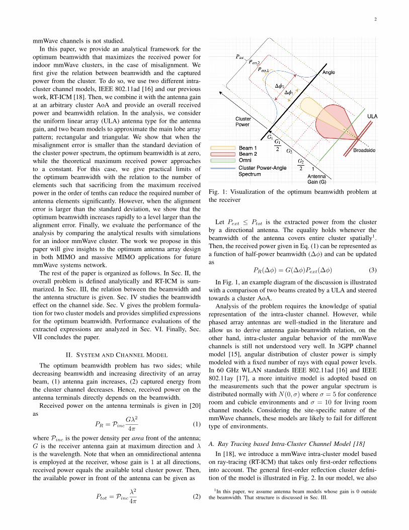
Fig. 1: Visualization of the optimum beamwidth problem atthe receiver

Let Pext ≤ Ptot is the extracted power from the clusterby a directional antenna. The equality holds whenever thebeamwidth of the antenna covers entire cluster spatially1.Then, the received power given in Eq. (1) can be represented asa function of half-power beamwidth (∆φ) and can be updatedas

PR(∆φ) = G(∆φ)Pext(∆φ) (3)

In Fig. 1, an example diagram of the discussion is illustratedwith a comparison of two beams created by a ULA and steeredtowards a cluster AoA.

Analysis of the problem requires the knowledge of spatialrepresentation of the intra-cluster channel. However, whilephased array antennas are well-studied in the literature andallow us to derive antenna gain-beamwidth relation, on theother hand, intra-cluster angular behavior of the mmWavechannels is still not understood very well. In 3GPP channelmodel [15], angular distribution of cluster power is simplymodeled with a fixed number of rays with equal power levels.In 60 GHz WLAN standards IEEE 802.11ad [16] and IEEE802.11ay [17], a more intuitive model is adopted based onthe measurements such that the power angular spectrum isdistributed normally with N(0, σ) where σ = 5 for conferenceroom and cubicle environments and σ = 10 for living roomchannel models. Considering the site-specific nature of themmWave channels, these models are likely to fail for differenttype of environments.

A. Ray Tracing based Intra-Cluster Channel Model [18]

In [18], we introduce a mmWave intra-cluster model basedon ray-tracing (RT-ICM) that takes only first-order reflectionsinto account. The general first-order reflection cluster defini-tion of the model is illustrated in Fig. 2. In our model, we also

1In this paper, we assume antenna beam models whose gain is 0 outsidethe beamwidth. That structure is discussed in Sec. III.

3

Fig. 2: First-order reflection cluster model of the RT-ICM

add the scattering effect based on the material properties. Itoutputs the power distribution both in angle and time domainwithin the cluster and can be used for both indoor and outdoormmWave systems in any type of stationary environments. Inspecific, the proposed cluster channel model comprises threemain steps; namely, basic geometry modeling, theoretical clus-ter modeling, and binned channel impulse response generation.First, Basic Geometric Model (BGM) takes first-order reflec-tion cluster environment parameters as inputs and generatesthe supported angle spread (SAS), Sφ = φmax − φmin, atthe receiver. Second, running the BGM for each infinitelylarge number of rays that are within the supported anglespread; angle, time, power and phase of the rays are calculated;thereby generating the theoretical cluster impulse response.The output theoretical baseband cluster impulse response (TC-CIR) is given by [18]

cT (tsp, φsp) = aspejϕspδ(tsp)δ(φsp)

+

Ndr−1∑k=0

akejϕkδ(tsp − τk)δ(φsp − αk)

(4)

where asp, ϕsp, tsp and φsp are the amplitude, phase, time ofarrival (ToA) and AoA of the specular ray, respectively; ak,ϕk, τk, αk are amplitude, phase, delay, offset AoA of the k-thray, respectively. δ(.) is Dirac delta function and Nd

r is thenumber of rays.

Finally, the theoretical impulse response is binned in theangle and time domain according to the bandwidth and angleresolution of the communication system. Basically, the binnedversion is the impulse response that the receiver sees. Wesimply call it cluster channel impulse response (C-CIR). Thediagram of the overall modeling process is given in Fig. 3.Note that, since we are interested in estimating the receivedpower at the antenna terminals in this paper, i.e. before receiversignal processing, we will use the theoretical impulse responsegiven in Eq. (4) as the cluster power angle profile. Then, thetotal power in the cluster is given as

Ptot = a2sp +

SφNdr

Ndr∑k=0

a2k (5)

Fig. 3: Flowchart diagram of the cluster channel impulseresponse generation.

Fig. 4: An example cluster power angle profile of RT-ICM.

where Sφ/Ndr term is inserted for the integral approximation.

An example of a cluster angle profile output of RT-ICM isdisplayed in Fig. 4 for Nd

r = 75 and Sφ = 75◦.

III. ANTENNA STRUCTURE AND GAIN

As Eq. (3) suggests, antenna gain is the counterpart ofthe captured cluster power in the equation for a certainbeamwidth. Finding an expression for antenna gain as afunction beamwidth for an arbitrary array design is not easyand out-of-scope of the paper. Instead, we adopt the well-known uniform linear array (ULA) design where the spacingsbetween the elements are equal and we seek to find therelationships between antenna gain, beamwidth, number ofelements and scan angle for a ULA.

A. Beam Pattern Model

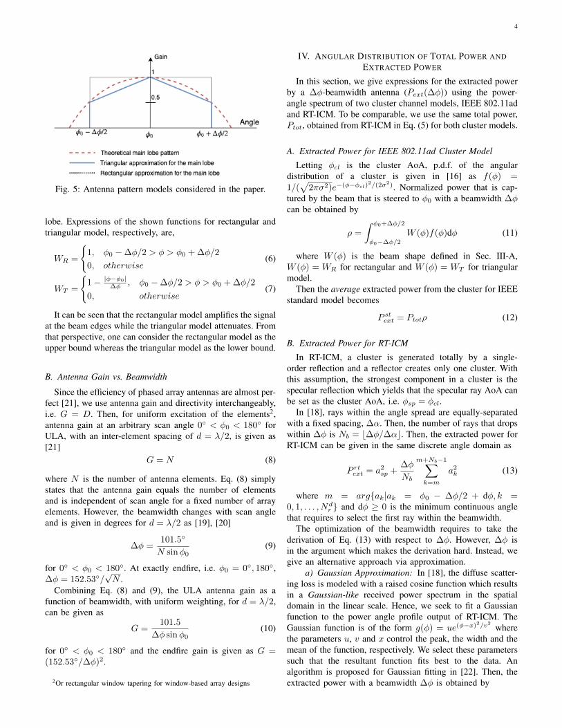
In this paper, we use two models for the beam pattern; arectangular window and a triangular window, both are seenin Fig. 5 for a steering (scan) angle of φ0. Both approxima-tions ignore the sidelobes; thereby modeling only the main

4

Fig. 5: Antenna pattern models considered in the paper.

lobe. Expressions of the shown functions for rectangular andtriangular model, respectively, are,

WR =

{1, φ0 −∆φ/2 > φ > φ0 + ∆φ/2

0, otherwise(6)

WT =

{1− |φ−φ0|

∆φ , φ0 −∆φ/2 > φ > φ0 + ∆φ/2

0, otherwise(7)

It can be seen that the rectangular model amplifies the signalat the beam edges while the triangular model attenuates. Fromthat perspective, one can consider the rectangular model as theupper bound whereas the triangular model as the lower bound.

B. Antenna Gain vs. Beamwidth

Since the efficiency of phased array antennas are almost per-fect [21], we use antenna gain and directivity interchangeably,i.e. G = D. Then, for uniform excitation of the elements2,antenna gain at an arbitrary scan angle 0◦ < φ0 < 180◦ forULA, with an inter-element spacing of d = λ/2, is given as[21]

G = N (8)

where N is the number of antenna elements. Eq. (8) simplystates that the antenna gain equals the number of elementsand is independent of scan angle for a fixed number of arrayelements. However, the beamwidth changes with scan angleand is given in degrees for d = λ/2 as [19], [20]

∆φ =101.5◦

N sinφ0(9)

for 0◦ < φ0 < 180◦. At exactly endfire, i.e. φ0 = 0◦, 180◦,∆φ = 152.53◦/

√N .

Combining Eq. (8) and (9), the ULA antenna gain as afunction of beamwidth, with uniform weighting, for d = λ/2,can be given as

G =101.5

∆φ sinφ0(10)

for 0◦ < φ0 < 180◦ and the endfire gain is given as G =(152.53◦/∆φ)2.

2Or rectangular window tapering for window-based array designs

IV. ANGULAR DISTRIBUTION OF TOTAL POWER ANDEXTRACTED POWER

In this section, we give expressions for the extracted powerby a ∆φ-beamwidth antenna (Pext(∆φ)) using the power-angle spectrum of two cluster channel models, IEEE 802.11adand RT-ICM. To be comparable, we use the same total power,Ptot, obtained from RT-ICM in Eq. (5) for both cluster models.

A. Extracted Power for IEEE 802.11ad Cluster Model

Letting φcl is the cluster AoA, p.d.f. of the angulardistribution of a cluster is given in [16] as f(φ) =1/(√

2πσ2)e−(φ−φcl)2/(2σ2). Normalized power that is cap-tured by the beam that is steered to φ0 with a beamwidth ∆φcan be obtained by

ρ =

∫ φ0+∆φ/2

φ0−∆φ/2

W (φ)f(φ)dφ (11)

where W (φ) is the beam shape defined in Sec. III-A,W (φ) = WR for rectangular and W (φ) = WT for triangularmodel.

Then the average extracted power from the cluster for IEEEstandard model becomes

P stext = Ptotρ (12)

B. Extracted Power for RT-ICM

In RT-ICM, a cluster is generated totally by a single-order reflection and a reflector creates only one cluster. Withthis assumption, the strongest component in a cluster is thespecular reflection which yields that the specular ray AoA canbe set as the cluster AoA, i.e. φsp = φcl.

In [18], rays within the angle spread are equally-separatedwith a fixed spacing, ∆α. Then, the number of rays that dropswithin ∆φ is Nb = b∆φ/∆αc. Then, the extracted power forRT-ICM can be given in the same discrete angle domain as

P rtext = a2sp +

∆φ

Nb

m+Nb−1∑k=m

a2k (13)

where m = arg{ak|ak = φ0 − ∆φ/2 + dφ, k =0, 1, . . . , Nd

r } and dφ ≥ 0 is the minimum continuous anglethat requires to select the first ray within the beamwidth.

The optimization of the beamwidth requires to take thederivation of Eq. (13) with respect to ∆φ. However, ∆φ isin the argument which makes the derivation hard. Instead, wegive an alternative approach via approximation.

a) Gaussian Approximation: In [18], the diffuse scatter-ing loss is modeled with a raised cosine function which resultsin a Gaussian-like received power spectrum in the spatialdomain in the linear scale. Hence, we seek to fit a Gaussianfunction to the power angle profile output of RT-ICM. TheGaussian function is of the form g(φ) = ue(φ−x)2/v2

wherethe parameters u, v and x control the peak, the width and themean of the function, respectively. We select these parameterssuch that the resultant function fits best to the data. Analgorithm is proposed for Gaussian fitting in [22]. Then, theextracted power with a beamwidth ∆φ is obtained by

5

P rtext =

∫ φ0+∆φ/2

φ0−∆φ/2

W (φ)g(φ)dφ (14)

V. PROBLEM FORMULATION

In case of an imperfect channel knowledge, cluster angle ofarrival, φcl, is estimated with an error. Additionally, a quan-tization error is introduced at the receiver when a codebookis implemented for beamforming. Then the total misalignmenterror at the receiver can be defined as3 δ = |φ0 − φcl|. Wefirst set up the problem formulation with W (φ) = WR.

A. IEEE 802.11ad

Plugging antenna gain and extracted power equations in Eq.(10) and (12), respectively, into Eq. (3),

PR(∆φ) =101.5◦

∆φ sinφ0Ptotρ (15)

where ρ is integral given in Eq. (11). From [23], the integrationof a Gaussian can be defined with the error function (erf ).Then,

ρ =

∫ φcl+δ+∆φ/2

φcl+δ−∆φ/2

WR(φ)1√

2πσ2e−

(φ−φcl)2

2σ2 dφ

=1

2

(erf(

∆φ+ 2δ

2√

2σ

)+ erf

(∆φ− 2δ

2√

2σ

))(16)

where erf(z) = 1√

2π∫ z

0e−y

2/2dy. Plugging into Eq. (15),the received power can be given as following:

PR(∆φ) =

50.75Ptot∆φ sinφ0

(erf(

∆φ+ 2δ

2√

2σ

)+ erf

(∆φ− 2δ

2√

2σ

))(17)

such that 0 < ∆φ.1) Maximization of PR: We seek to find the optimum

∆φ = ∆φopt that maximizes the Eq. (17). Since Ptot andsinφ0 are positive and scaling doesn’t affect the optimization,the problem can be reduced to the following:

maxerf(

∆φ+2δ

2√

2σ

)+ erf

(∆φ−2δ

2√

2σ

)∆φ

(18)

Making an argument whether the Eq. (18) is concave is notstraightforward. To investigate the concavity of the function,we apply Second Derivative Test which is summarized asfollows. If q′(z0) = 0 and q′′(z0) < 0, then z0 is thelocal maximum of the function q(z). The simplified conditionsderived from the first and the second derivatives of the Eq. (18)are given in Eq. (19) and (20) at the top of page 6, respectively.The details are placed in Appendix A.

Due to the erf function, no closed-form is available for Eq.(19), thus, solving it for ∆φ > 0 is performed numerically,for fixed δ and σ. The function has always 2 roots, one at theinfinity. Plugging the roots to Eq. (20), it can be seen that the

3Absolute value is inserted to keep the error positive as all the functionsused in the analysis are symmetric.

condition fails for the infinity root. Furthermore, it is counter-intuitive to have the infinitely large ∆φopt for the maximizedreceived power. In fact, this root is the local minimum of thefunction which minimizes the received power.

An example simulation of the PR in linear scale with respectto ∆φ for different δ values are given in Fig. 6 where Ptot =1.2µW , σ = 5◦ and φ0 = 53◦. It can be seen that the secondderivative test would result in the single local maximum, i.e.,global maximum. This leads to the following remark.

Remark 1: There exists a unique ∆φ > 0 that satistifiesthe both conditions in Eq. (19) and (20) for the given δ and σsuch that δ > σ. This unique value is the optimum beamwidth,∆φopt, that maximizes the received power for the given δ andσ.

Also, to be proven in the simulation results in Sec. VI, wepropose another important remark:

Remark 2: The following statements are always true. (1)When δ >

√2σ, ∆φopt > 2δ, (2) When δ ≤ σ, ∆φopt = 0.

To get the insight of the results, consider the diagram givenin Fig. 7. The relation between δ and σ has a significant effecton the value of ∆φopt. As long as δ ≤ σ, it is enough for theantenna to capture a little from the first σ region of the channelspectrum and antenna gain dominates the maximum receivedpower. However, once δ > σ, channel gain that is capturedfrom the tail is considerably small such that even the antennagain cannot tolerate. Hence, regardless of δ, the maximumreceived power is achieved only when the beam captures fromthe first σ region of the channel spectrum. Furthermore, ifδ >√

2σ, beam should cover the center of the cluster. Thatis, ∆φopt/2 > δ, or ∆φopt > 2δ.

Finally, once optimum beamwidth is determined, maximumreceived power can be obtained by plugging ∆φopt into Eq.(17),

Pmax = PR(∆φopt) (21)

B. RT-ICM

Apparently, the equations, given in Eq. (12) and (14), areequal with different notations. Hence, skipping the intermedi-ate steps, received power for RT-ICM is given as

P rtR (∆φ) =

50.75uv√π

∆φ sinφ0

(erf(

∆φ+ 2δ

2v

)+ erf

(∆φ− 2δ

2v

))(22)

Maximization procedure of P rtR (∆φ) is analogous to the802.11ad case. In fact, setting σ = v/

√2 in Eq. (19) and

(20), conditions for RT-ICM can be provided.Note that the IEEE 802.11ad standard sets σ to a fixed value

for specific environments whereas RT-ICM generates differentv for each cluster. In any way, after getting v, one can convertit to σ and use the same notation with 802.11ad.

6

∆φ(e−(∆φ+2δ)2/8σ2

+ e−(∆φ−2δ)2/8σ2)− σ√

2π

(erf(

∆φ+ 2δ

2√

2σ

)+ erf

(∆φ− 2δ

2√

2σ

))= 0 (19)

∆φ(∆φ(∆φ+ 2δ) + 8σ2)

e(∆φ+2δ)2/8σ2 +∆φ(∆φ(∆φ− 2δ) + 8σ2)

e(∆φ−2δ)2/8σ2 >

(erf(

∆φ+ 2δ

2√

2σ

)+ erf

(∆φ− 2δ

2√

2σ

))(20)

Fig. 6: Received power in case of misalignment for σ = 5 andPtot = 1.2µW .

Fig. 7: Optimum beamwidth in case of misalignment.

C. Asymptotic Analysis of Perfect Alignment

It is already shown that ∆φopt = 0 when δ ≤ σ. Note thatinfinitely many elements (N = ∞) are required to achieve∆φopt = 0, which is impractical. In this section, we performan asymptotic analysis of the maximum achievable receivedpower while ∆φopt → 0 and provide an expression that resultsin practical beamwidth values that captures a percentile of themaximum achievable power. We perform the analysis with the802.11ad model but give the counterpart expressions for RT-ICM at the end of the section as well.

To simplify the analysis and create a generic expression forany σ, let us assume δ = 0, i.e. φ0 = φcl. Then from Eq. (11),for W (φ) = WR, ρ becomes4,

4It can also be verified by plugging δ = 0 in Eq. (16).

ρ = erf(

∆φ

2√

2σ

)(23)

Plugging into Eq. (15), received power equation simplifiesto,

PR(∆φ) =101.5Ptot∆φ sinφ0

erf(

∆φ

2√

2σ

)(24)

1) Maximum Received Power: We now seek to find themaximum received power as the limit ∆φ→ 0. Eq. (24) is inthe 0/0 indeterminate form for ∆φ = 0. Applying L’Hopitalrule, the maximum achievable received power is

P tmax = PR(0) =40.5Ptotσ sinφ0

(25)

Intermediate steps are given in the Appendix B.2) Optimum Practical Beamwidth: Note that the maximum

received power given in the Eq. (25) is theoretical. Achievingvery small beamwidth requires impractically high number ofantenna elements as the relation given in Eq. (9) suggests.However, we can keep the beamwidth in practical ranges whilesacrificing subtle from the received power.

Let 0 < η ≤ 1 be the coefficient such that

P tη = ηP tmax (26)

where P tη is the η-percentile power of the P tmax. Then, fromEq. (24),

101.5Ptot∆φ sinφ0

erf(

∆φ

2√

2σ

)= P stη = η

40.5Ptotσ sinφ0

(27)

Simplifying the equation and setting ∆φ = ∆φη , i.e.practical η-percentile beamwidth,

∆φη

erf(

∆φη2√

2σ

) =2.5σ

η(28)

Similar to the imperfect alignment case in Eq. (18), Eq.(28) shows that the optimum beamwidth depends only on theangle spread of the cluster while total cluster power and thescan angle has no effect at all. However, different from theimperfect alignment, an approximate solution can be providedfor Eq. (28). Expanding the erf(z) function to Taylor seriessuch that erf(z) = 2

(z − z3/3 + z5/10− z7/42 + . . .

)/√π

where z = ∆φ/√

8σ, we can approximate it ignoring the highorder terms when ∆φ/

√8σ < 1. Referring to Appendix B

for the derivation, the η-percentile beamwidth can be given,approximately,

∆φη ≈ 4.89 σ√

1− η (29)

As shown in the simulation results section, Eq. (29) providesa strong yet simple tool to determine the optimum beamwidth

7

TABLE I: Asymptotic Analysis of Pmax and PerformanceComparison of 802.11ad and RT-ICM

η-percentile ∆φst Nst ∆φrt Nrt

0.999 0.8◦ 166 1.0◦ 1260.99 2.5◦ 52 3.2◦ 400.95 5.6◦ 23 7.3◦ 180.9 8.1◦ 16 10.6◦ 120.75 14.0◦ 10 18.3◦ 70.5 24.7◦ 6 32.3◦ 4

within the practical limits. However, once ∆φ >√

8σ,approximation of the error function starts getting apart fromthe real value. Setting ∆φ ≤

√8σ as the support region of

∆φ, from Eq. (29),

4.89 σ√

1− η ≤√

8σ

η ≥ 0.667 (30)

which provides the lower bound accuracy limit of the Eq. (29).Finally, to prove that Eq. (29) results in practical beamwidthvalues for conference room environments, from Eq. (30) and(33), beamwidth is given in the support range of ∆φη ≤ 14.10which can be achieved at the broadside using N ≥ 8 antennaelements.

Plugging the given standard deviation for conference roomenvironments [16] σ = 5, Eq. (25), (28) and (29) becomes

P stmax =8.1Ptotsinφ0

(31)

∆φst

erf(

∆φst

10√

2

) =12.5

η(32)

∆φst = 24.45√

1− η (33)

Due to the similar discussion made in Sec. V-B, we justgive the RT-ICM counterpart expressions here. With notationchanges, received power equation becomes

P rtR (∆φ) =101.5◦uv

√π

∆φ sinφ0erf(

∆φ

2v

)(34)

The maximum received power for the RT-ICM is

P rtmax =101.5u

sinφ0(35)

Exact equation for the practical η-percentile beamwidth,∆φη , for the RT-ICM,

∆φrt

erf(

∆φrt

2v

) =v√π

η(36)

and its approximation for ∆φ ≤ 2v,

∆φrt ≈ 3.46 v√

1− η (37)

Table I shows a case study with a cluster in a typical indoorenvironment. The total power, Ptot in dBm is calculated viaRT-ICM to be −29.09. Scan angle is, φ0 = 53◦ and SASis Sφ = 72.2◦. Corresponding Gaussian fitting parametersfor RT-ICM are u = 6.43 × 10−5 and v = 9.23 (orσ = 9.23/

√2 = 6.52). Then, from Eq. (31) and (35), and

converting to dBm, P stmax = −19.15 and P rtmax = −20.87 bothin dBm. In Table I, we calculate ∆φst and ∆φrt numericallyusing Eq. (32) and (36), respectively. Associated requirednumber of elements to create the beamwidths, Nst and Nrt

are computed using Eq. (9). While infinite number of antennaelements are required to achieve asymptotic values of thereceived power, Table I shows that high percentile powers canbe obtained via practical values of N . On the other hand, it canbe seen that for η ≥ 0.95, in spite of the beamwidth differencebetween 802.11ad and RT-ICM is subtle, the difference inthe required number of elements is increasing significantly.That proves that the hardware complexity to achieve optimumbeamwidth value is directly related (and sensitive) to thecorrect estimation of the cluster parameters such as anglespread.

D. Triangular Beam Model

Throughout the paper, we used the rectangular beam modelgiven in Eq. (6) so far for all the analysis. In this section, weupdate the main equations for triangular beam model givenin Eq. (7) and provide the difference with respect to therectangular beam model.

Remark 3: Following statements are true for both perfectand imperfect alignments: (1) ∆φopt doesn’t depend on themain lobe beam model. (2) The difference in maximumachievable power is 1.23 dB.

Starting from the perfect alignment, Eq. (11) is calculatedas following:

ρ =

∫ φcl+∆φ/2

φcl−∆φ/2

WT f(φ)dφ

= erf(

∆φ

2√

2σ

)−√

2(1− e−∆φ2/8σ2

)√π∆φ

(38)

Plugging into Eq. (12), skipping intermediate steps, receivedpower is obtained as

PR(∆φ) =101.5Ptot∆φ sinφ0

erf(

∆φ

2√

2σ

)−81Ptotσ(1− e−∆φ2/8σ2

)

sinφ0∆φ2

(39)Note that the first term is the PR(∆φ) for the rectangular

beam model given in Eq. (24) which is maximum at ∆φ = 0.On the other hand, the second term is always positive andminimized at ∆φ = 0. This proves that the Pmax is at ∆φ = 0.Taking the limit while ∆φ → 0, theoretical maximum powerwith the triangular model is

P tT,max = PR(0) =30.5Ptotσ sinφ0

(40)

Comparing with the rectangular model in Eq. (25), thedifference is

10 log(P tmax/P

tT,max

)= 1.23 dB (41)

Since the result doesn’t depend on any parameter, it is alsotrue for the RT-ICM case.

The proof for the imperfect alignment is performed viasimulation as the difference equation is computed numericallydue to the erf.

8

Fig. 8: Accuracy of second derivative test method in case ofmisalignment and δ − σ relation effect on ∆φopt.

VI. PERFORMANCE EVALUATION

In this section, we give the plots that illustrate the perfor-mance of the given analytical expressions by comparing withthe simulations. We use the 802.11ad Gaussian notation forthe performance results, but, to show the difference betweenfixed versus exact σ, we refer 802.11ad for fixed, RT-ICMfor the true value. As both models agree for indoor mmWaveclusters, we scan a range of 3◦ to 10◦ for σ.

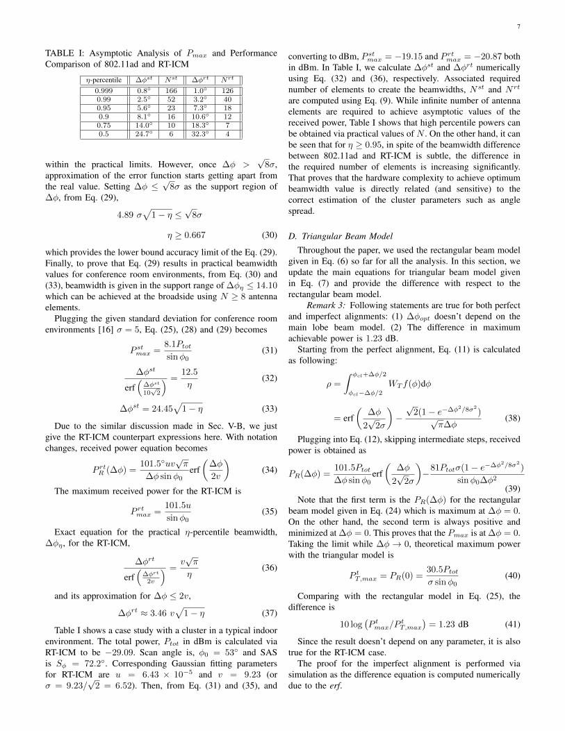
In the first plot, we measure the accuracy of the methodthat uses the Second Derivative Test when finding the ∆φoptin case of misalignment, given in Sec. V-A1. As seen from Fig.8, optimization results for ∆φopt perfectly match to simulationresults for different values of σ and δ, as stated in Remark 1.On the other hand, note that ∆φopt → 0 rapidly while δ ≈ σ.Also, it can be seen that ∆φopt > 2δ once δ ≥

√2σ. This

concludes the proof of Remark 2.Fig. 9 shows how the maximum received power given in Eq.

(21) changes in dB scale with variation in δ for four differentσs. In the figure, the received power is normalized with Ptot.As seen, once δ > σ, Pmax drops exponentially and becomesthe dominant degradation factor. However, even with a largeδ, using a ULA has still advantages over an omnidirectionalantenna. On the other hand, as δ ≈ σ, Pmax reaches to itsmax level. Although not shown here, for δ < σ, it saturatesrapidly, which can be concluded from Fig. 6. That results inthe following important conclusion: As long as δ < σ, themisalignment error is tolerable thanks to the antenna gain andmaximum power can be still achieved.

Fig. 9 also shows the effect of the steering angle φ0 to Pmaxfor σ = 5. As seen, Pmax strictly depends on φ0 due to thesin factor in the denominator. However, recall that since φ0

depends on the channel parameter φcl, user has limited controlover it.

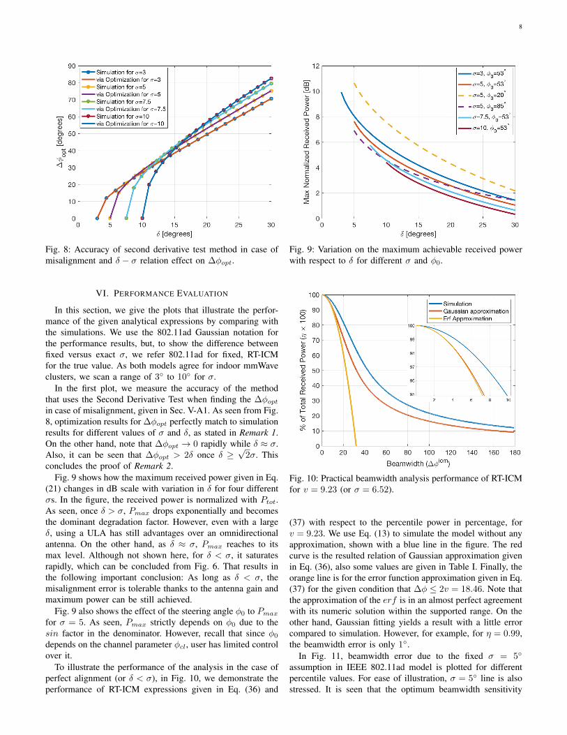
To illustrate the performance of the analysis in the case ofperfect alignment (or δ < σ), in Fig. 10, we demonstrate theperformance of RT-ICM expressions given in Eq. (36) and

Fig. 9: Variation on the maximum achievable received powerwith respect to δ for different σ and φ0.

Fig. 10: Practical beamwidth analysis performance of RT-ICMfor v = 9.23 (or σ = 6.52).

(37) with respect to the percentile power in percentage, forv = 9.23. We use Eq. (13) to simulate the model without anyapproximation, shown with a blue line in the figure. The redcurve is the resulted relation of Gaussian approximation givenin Eq. (36), also some values are given in Table I. Finally, theorange line is for the error function approximation given in Eq.(37) for the given condition that ∆φ ≤ 2v = 18.46. Note thatthe approximation of the erf is in an almost perfect agreementwith its numeric solution within the supported range. On theother hand, Gaussian fitting yields a result with a little errorcompared to simulation. However, for example, for η = 0.99,the beamwidth error is only 1◦.

In Fig. 11, beamwidth error due to the fixed σ = 5◦

assumption in IEEE 802.11ad model is plotted for differentpercentile values. For ease of illustration, σ = 5◦ line is alsostressed. It is seen that the optimum beamwidth sensitivity

9

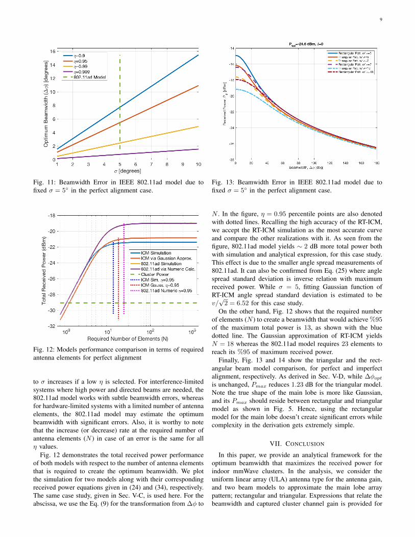
Fig. 11: Beamwidth Error in IEEE 802.11ad model due tofixed σ = 5◦ in the perfect alignment case.

Fig. 12: Models performance comparison in terms of requiredantenna elements for perfect alignment

to σ increases if a low η is selected. For interference-limitedsystems where high power and directed beams are needed, the802.11ad model works with subtle beamwidth errors, whereasfor hardware-limited systems with a limited number of antennaelements, the 802.11ad model may estimate the optimumbeamwidth with significant errors. Also, it is worthy to notethat the increase (or decrease) rate at the required number ofantenna elements (N ) in case of an error is the same for allη values.

Fig. 12 demonstrates the total received power performanceof both models with respect to the number of antenna elementsthat is required to create the optimum beamwidth. We plotthe simulation for two models along with their correspondingreceived power equations given in (24) and (34), respectively.The same case study, given in Sec. V-C, is used here. For theabscissa, we use the Eq. (9) for the transformation from ∆φ to

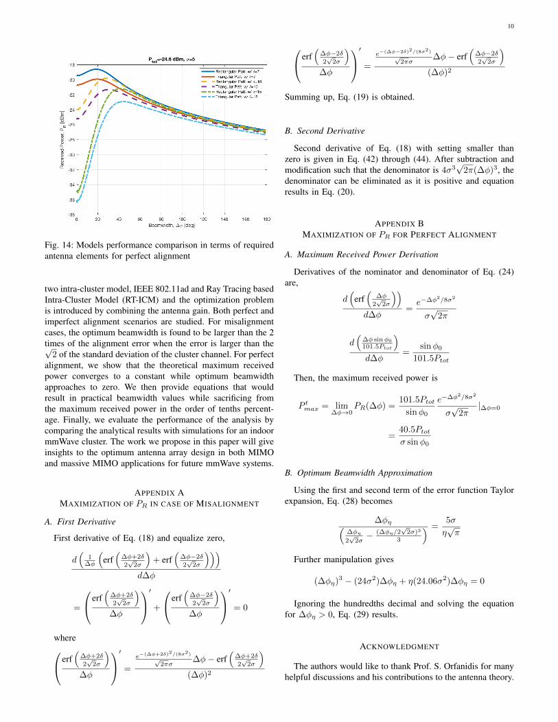
Fig. 13: Beamwidth Error in IEEE 802.11ad model due tofixed σ = 5◦ in the perfect alignment case.

N . In the figure, η = 0.95 percentile points are also denotedwith dotted lines. Recalling the high accuracy of the RT-ICM,we accept the RT-ICM simulation as the most accurate curveand compare the other realizations with it. As seen from thefigure, 802.11ad model yields ∼ 2 dB more total power bothwith simulation and analytical expression, for this case study.This effect is due to the smaller angle spread measurements of802.11ad. It can also be confirmed from Eq. (25) where anglespread standard deviation is inverse relation with maximumreceived power. While σ = 5, fitting Gaussian function ofRT-ICM angle spread standard deviation is estimated to bev/√

2 = 6.52 for this case study.On the other hand, Fig. 12 shows that the required number

of elements (N ) to create a beamwidth that would achieve %95of the maximum total power is 13, as shown with the bluedotted line. The Gaussian approximation of RT-ICM yieldsN = 18 whereas the 802.11ad model requires 23 elements toreach its %95 of maximum received power.

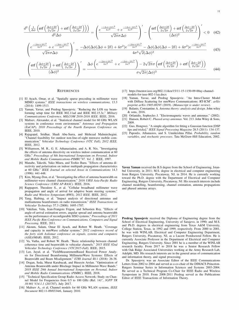
Finally, Fig. 13 and 14 show the triangular and the rect-angular beam model comparison, for perfect and imperfectalignment, respectively. As derived in Sec. V-D, while ∆φoptis unchanged, Pmax reduces 1.23 dB for the triangular model.Note the true shape of the main lobe is more like Gaussian,and its Pmax should reside between rectangular and triangularmodel as shown in Fig. 5. Hence, using the rectangularmodel for the main lobe doesn’t create significant errors whilecomplexity in the derivation gets extremely simple.

VII. CONCLUSION

In this paper, we provide an analytical framework for theoptimum beamwidth that maximizes the received power forindoor mmWave clusters. In the analysis, we consider theuniform linear array (ULA) antenna type for the antenna gain,and two beam models to approximate the main lobe arraypattern; rectangular and triangular. Expressions that relate thebeamwidth and captured cluster channel gain is provided for

10

Fig. 14: Models performance comparison in terms of requiredantenna elements for perfect alignment

two intra-cluster model, IEEE 802.11ad and Ray Tracing basedIntra-Cluster Model (RT-ICM) and the optimization problemis introduced by combining the antenna gain. Both perfect andimperfect alignment scenarios are studied. For misalignmentcases, the optimum beamwidth is found to be larger than the 2times of the alignment error when the error is larger than the√

2 of the standard deviation of the cluster channel. For perfectalignment, we show that the theoretical maximum receivedpower converges to a constant while optimum beamwidthapproaches to zero. We then provide equations that wouldresult in practical beamwidth values while sacrificing fromthe maximum received power in the order of tenths percent-age. Finally, we evaluate the performance of the analysis bycomparing the analytical results with simulations for an indoormmWave cluster. The work we propose in this paper will giveinsights to the optimum antenna array design in both MIMOand massive MIMO applications for future mmWave systems.

APPENDIX AMAXIMIZATION OF PR IN CASE OF MISALIGNMENT

A. First Derivative

First derivative of Eq. (18) and equalize zero,

d(

1∆φ

(erf(

∆φ+2δ

2√

2σ

)+ erf

(∆φ−2δ

2√

2σ

)))d∆φ

=

erf(

∆φ+2δ

2√

2σ

)∆φ

′ +erf

(∆φ−2δ

2√

2σ

)∆φ

′ = 0

whereerf(

∆φ+2δ

2√

2σ

)∆φ

′ =

e−(∆φ+2δ)2/(8σ2)√

2πσ∆φ− erf

(∆φ+2δ

2√

2σ

)(∆φ)2

erf(

∆φ−2δ

2√

2σ

)∆φ

′ =

e−(∆φ−2δ)2/(8σ2)√

2πσ∆φ− erf

(∆φ−2δ

2√

2σ

)(∆φ)2

Summing up, Eq. (19) is obtained.

B. Second Derivative

Second derivative of Eq. (18) with setting smaller thanzero is given in Eq. (42) through (44). After subtraction andmodification such that the denominator is 4σ3

√2π(∆φ)3, the

denominator can be eliminated as it is positive and equationresults in Eq. (20).

APPENDIX BMAXIMIZATION OF PR FOR PERFECT ALIGNMENT

A. Maximum Received Power Derivation

Derivatives of the nominator and denominator of Eq. (24)are,

d(

erf(

∆φ

2√

2σ

))d∆φ

=e−∆φ2/8σ2

σ√

2π

d(

∆φ sinφ0

101.5Ptot

)d∆φ

=sinφ0

101.5Ptot

Then, the maximum received power is

P tmax = lim∆φ→0

PR(∆φ) =101.5Ptot

sinφ0

e−∆φ2/8σ2

σ√

2π|∆φ=0

=40.5Ptotσ sinφ0

B. Optimum Beamwidth Approximation

Using the first and second term of the error function Taylorexpansion, Eq. (28) becomes

∆φη(∆φη2√

2σ− (∆φη/2

√2σ)3

3

) =5σ

η√π

Further manipulation gives

(∆φη)3 − (24σ2)∆φη + η(24.06σ2)∆φη = 0

Ignoring the hundredths decimal and solving the equationfor ∆φη > 0, Eq. (29) results.

ACKNOWLEDGMENT

The authors would like to thank Prof. S. Orfanidis for manyhelpful discussions and his contributions to the antenna theory.

11

d2(

1∆φ

(erf(

∆φ+2δ

2√

2σ

)+ erf

(∆φ−2δ

2√

2σ

)))d2∆φ

=

e−(∆φ+2δ)2

8σ2 + e−(∆φ−2δ)2

8σ2

√2πσ∆φ

′ −erf

(∆φ+2δ

2√

2σ

)+ erf

(∆φ−2δ

2√

2σ

)(∆φ)2

′ < 0 (42)

e−(∆φ+2δ)2

8σ2 + e−(∆φ−2δ)2

8σ2

√2πσ∆φ

′ =−∆φ(∆φ(∆φ+ 2δ) + 4σ2)e

−(∆φ+2δ)2

8σ2 −∆φ(∆φ(∆φ− 2δ) + 4σ2)e−(∆φ−2δ)2

8σ2

4σ3√

2(∆φ)2(43)

erf(

∆φ+2δ

2√

2σ

)+ erf

(∆φ−2δ

2√

2σ

)(∆φ)2

′ =

∆φ

(e

−(∆φ+2δ)2

8σ2 + e−(∆φ−2δ)2

8σ2

)− 2√

2πσ(

erf(

∆φ+2δ

2√

2σ

)+ erf

(∆φ−2δ

2√

2σ

))σ√

2π(∆φ)3(44)

REFERENCES

[1] El Ayach, Omar, et al. ”Spatially sparse precoding in millimeter waveMIMO systems.” IEEE transactions on wireless communications, 13.3(2014): 1499-1513.

[2] Yaman, Yavuz, and Predrag Spasojevic. ”Reducing the LOS ray beam-forming setup time for IEEE 802.11ad and IEEE 802.15.3c.” MilitaryCommunications Conference, MILCOM 2016-2016 IEEE. IEEE, 2016.

[3] Maltsev, Alexander, et al. ”Statistical channel model for 60 GHz WLANsystems in conference room environment.” Antennas and Propagation(EuCAP), 2010 Proceedings of the Fourth European Conference on.IEEE, 2010.

[4] Rajagopal, Sridhar, Shadi Abu-Surra, and Mehrzad Malmirchegini.”Channel feasibility for outdoor non-line-of-sight mmwave mobile com-munication.” Vehicular Technology Conference (VTC Fall), 2012 IEEE.IEEE, 2012.

[5] Williamson, M. R., G. E. Athanasiadou, and A. R. Nix. ”Investigatingthe effects of antenna directivity on wireless indoor communication at 60GHz.” Proceedings of 8th International Symposium on Personal, Indoorand Mobile Radio Communications-PIMRC’97. Vol. 2. IEEE, 1997.

[6] Manabe, Takeshi, Yuko Miura, and Toshio Ihara. ”Effects of antenna di-rectivity and polarization on indoor multipath propagation characteristicsat 60 GHz.” IEEE Journal on selected Areas in Communications 14.3(1996): 441-448.

[7] Kim, Myung-Don, et al. ”Investigating the effect of antenna beamwidth onmillimeter-wave channel charaterization.” 2016 URSI Asia-Pacific RadioScience Conference (URSI AP-RASC). IEEE, 2016.

[8] Rappaport, Theodore S., et al. ”Cellular broadband millimeter wavepropagation and angle of arrival for adaptive beam steering systems.”Radio and Wireless Symposium (RWS), 2012 IEEE. IEEE, 2012.

[9] Yang, Haibing, et al. ”Impact analysis of directional antennas andmultiantenna beamformers on radio transmission.” IEEE Transactions onVehicular Technology 57.3 (2008): 1695-1707.

[10] Vakilian, Vida, Jean-Frangois Frigon, and Sebastien Roy. ”Effects ofangle-of-arrival estimation errors, angular spread and antenna beamwidthon the performance of reconfigurable SISO systems.” Proceedings of 2011IEEE Pacific Rim Conference on Communications, Computers and SignalProcessing. IEEE, 2011.

[11] Akoum, Salam, Omar El Ayach, and Robert W. Heath. ”Coverageand capacity in mmWave cellular systems.” 2012 conference record ofthe forty sixth Asilomar conference on signals, systems and computers(ASILOMAR). IEEE, 2012.

[12] Va, Vutha, and Robert W. Heath. ”Basic relationship between channelcoherence time and beamwidth in vehicular channels.” 2015 IEEE 82ndVehicular Technology Conference (VTC2015-Fall). IEEE, 2015.

[13] Lee, Juyul, et al. ”FieldMeasurementBased Received Power Analy-sis for Directional Beamforming MillimeterWave Systems: Effects ofBeamwidth and Beam Misalignment.” ETRI Journal 40.1 (2018): 26-38.

[14] Dogan, Seda, Murat Karabacak, and Huseyin Arslan. ”Optimization ofAntenna Beamwidth under Blockage Impact in Millimeter-Wave Bands.”2018 IEEE 29th Annual International Symposium on Personal, Indoorand Mobile Radio Communications (PIMRC). IEEE, 2018.

[15] ”Technical Specification Group Radio Access Network; Study on Chan-nel Model for Frequencies from 0.5 to 100 GHz (Rel. 14)”, 3GPP TR38.901 V14.1.1 (201707), July 2017.

[16] Maltsev A., et al, Channel models for 60 GHz WLAN systems, IEEEDocument 802.11-09/0334r6, January 2010.

[17] https://mentor.ieee.org/802.11/dcn/15/11-15-1150-09-00ay-channel-models-for-ieee-802-11ay.docx

[18] Yaman, Yavuz, and Predrag Spasojevic. ”An Intra-Cluster Modelwith Diffuse Scattering for mmWave Communications: RT-ICM”. arXivpreprint arXiv:1905.08295 (2019). (Manuscript is under review).

[19] Balanis, Constantine A. Antenna theory: analysis and design. John wiley& sons, 2016.

[20] Orfanidis, Sophocles J. ”Electromagnetic waves and antennas.” (2002).[21] Hansen, Robert C. Phased array antennas. Vol. 213. John Wiley & Sons,

2009.[22] Guo, Hongwei. ”A simple algorithm for fitting a Gaussian function [DSP

tips and tricks].” IEEE Signal Processing Magazine 28.5 (2011): 134-137.[23] Papoulis, Athanasios, and S. Unnikrishna Pillai. Probability, random

variables, and stochastic processes. Tata McGraw-Hill Education, 2002.

Yavuz Yaman received the B.S degree from the School of Engineering, Istan-bul University, in 2011; M.S. degree in electrical and computer engineeringfrom Rutgers University, Piscataway, NJ, in 2014. He is currently workingtoward the Ph.D. degree with the Department of Electrical and ComputerEngineering, Rutgers University, Piscataway, NJ. His research interests includechannel modelling, beamforming, channel estimation, antenna propagationsand phased antenna arrays.

Predrag Spasojevic received the Diploma of Engineering degree from theSchool of Electrical Engineering, University of Sarajevo, in 1990; and M.S.and Ph.D. degrees in electrical engineering from Texas A&M University,College Station, Texas, in 1992 and 1999, respectively. From 2000 to 2001,he was with WINLAB, Electrical and Computer Engineering Department,Rutgers University, Piscataway, NJ, as a Lucent Postdoctoral Fellow. He iscurrently Associate Professor in the Department of Electrical and ComputerEngineering, Rutgers University. Since 2001 he is a member of the WINLABresearch faculty. From 2017 to 2018 he was a Senior Research Fellowwith Oak Ridge Associated Universities working at the Army Research Lab,Adelphi, MD. His research interests are in the general areas of communicationand information theory, and signal processing.

Dr. Spasojevic was an Associate Editor of the IEEE CommunicationsLetters from 2002 to 2004 and served as a co-chair of the DIMACS Princeton-Rutgers Seminar Series in Information Sciences and Systems 2003-2004.He served as a Technical Program Co-Chair for IEEE Radio and WirelessSymposium in 2010. From 2008-2011 Predrag served as the PublicationsEditor of IEEE Transactions of Information Theory.