The Impact of Beamwidth on Temporal Channel Variation in...

Technical Report 107

The Impact of Beamwidth on Temporal Channel Variation in Vehicular Channels and its Implications Vutha Va Junil Choi Robert W. Heath Jr. Wireless Networking and Communications Group November 2015 Project title: Coherence Time and Beam Alignment for mmWave Vehicular Communications

Data-Supported Transportation Operations & Planning Center (D-STOP)

A Tier 1 USDOT University Transportation Center at The University of Texas at Austin

D-STOP is a collaborative initiative by researchers at the Center for Transportation Research and the Wireless Networking and Communications Group at The University of Texas at Austin.

DISCLAIMER The contents of this report reflect the views of the authors, who are responsible for the facts and the accuracy of the information presented herein. This document is disseminated under the sponsorship of the U.S. Department of Transportation’s University Transportation Centers Program, in the interest of information exchange. The U.S. Government assumes no liability for the contents or use thereof.

Technical Report Documentation Page

1. Report No.

D-STOP/2016/107 2. Government Accession No.

3. Recipient's Catalog No.

4. Title and Subtitle

The Impact of Beamwidth on Temporal Channel Variation in Vehicular Channels and its Implications

5. Report Date

November2015 6. Performing Organization Code

7. Author(s)

Vutha Va, Junil Choi, and Robert W. Heath Jr. 8. Performing Organization Report No.

Report 107 9. Performing Organization Name and Address

Data-Supported Transportation Operations & Planning Center (D-STOP) The University of Texas at Austin 1616 Guadalupe Street, Suite 4.202 Austin, Texas 78701

10. Work Unit No. (TRAIS)

11. Contract or Grant No.

DTRT13-G-UTC58

12. Sponsoring Agency Name and Address

Data-Supported Transportation Operations & Planning Center (D-STOP) The University of Texas at Austin 1616 Guadalupe Street, Suite 4.202 Austin, Texas 78701

13. Type of Report and Period Covered

14. Sponsoring Agency Code

15. Supplementary Notes

Supported by a grant from the U.S. Department of Transportation, University Transportation Centers Program. Project Name: Coherence Time and Beam Alignment for mmWave Vehicular Communications 16. Abstract

Millimeter wave (mmWave) has great potential in realizing high data rate thanks to the large spectral channels. It is considered as a key technology for the fifth generation wireless networks and is already used in wireless LAN (e.g., IEEE 802.11ad). Using mmWave for vehicular communications, however, is often viewed with some skepticism due to a misconception that the Doppler spread would become too large at these high frequencies. This is not true when directional beam is employed for communications. In this paper, closed form expressions relating the channel coherence time and beamwidth are derived. Unlike prior work that assumed perfect beam pointing, the pointing error due to the receiver motion is incorporated to show that there exists a non-zero optimal beamwidth that maximizes the coherence time. To investigate the mobility effect on the beam alignment which is an important feature in mmWave systems, a novel concept of beam coherence time is defined. The beam coherence time, which is an effective measure of beam alignment frequency, is shown to be much larger than the conventional channel coherence time and thus results in reduced beam alignment overhead. Using the derived correlation function, the channel coherence time, and the beam coherence time, an overall performance metric considering both the channel time-variation and the beam alignment overhead is derived. Using this metric, it is shown that beam alignment in every beam coherence time performs better than the beam alignment in every channel coherence time due to the large overhead for the latter case. 17. Key Words

Channel coherence time, Vehicular communication, Doppler spread, Millimeter wave, Beam alignment, Beamforming

18. Distribution Statement

No restrictions. This document is available to the public through NTIS (http://www.ntis.gov):

National Technical Information Service 5285 Port Royal Road Springfield, Virginia 22161

19. Security Classif.(of this report)

Unclassified 20. Security Classif.(of this page)

Unclassified 21. No. of Pages

22. Price

Form DOT F 1700.7 (8‐72) Reproduction of completed page authorized

iv

Disclaimer

The contents of this report reflect the views of the authors, who are responsible for the facts and the accuracy of the information presented herein. Mention of trade names or commercial products does not constitute endorsement or recommendation for use.

Acknowledgements

This material is based upon work supported in part by the National Science Foundation under Grant No. NSF-CCF-1319556, the U.S. Department of Transportation through the Data-Supported Transportation Operations and Planning (D-STOP) Tier 1 University Transportation Center, the Texas Department of Transportation under Project 0-6877 entitled “Communications and Radar-Supported Transportation Operations and Planning (CAR-STOP),” and by a gift from TOYOTA InfoTechnology Center, U.S.A., Inc. Part of this work was presented at the 2015 IEEE 82nd Vehicular Technology Conference in September 2015.

.

1

The Impact of Beamwidth on Temporal

Channel Variation in Vehicular Channels and

its Implications

Vutha Va, Junil Choi, and Robert W. Heath Jr.

Abstract

Millimeter wave (mmWave) has great potential in realizing high data rate thanks to the large spectral

channels. It is considered as a key technology for the fifth generation wireless networks and is already

used in wireless LAN (e.g., IEEE 802.11ad). Using mmWave for vehicular communications, however,

is often viewed with some skepticism due to a misconception that the Doppler spread would become too

large at these high frequencies. This is not true when directional beam is employed for communications.

In this paper, closed form expressions relating the channel coherence time and beamwidth are derived.

Unlike prior work that assumed perfect beam pointing, the pointing error due to the receiver motion is

incorporated to show that there exists a non-zero optimal beamwidth that maximizes the coherence time.

To investigate the mobility effect on the beam alignment which is an important feature in mmWave

systems, a novel concept of beam coherence time is defined. The beam coherence time, which is an

effective measure of beam alignment frequency, is shown to be much larger than the conventional channel

coherence time and thus results in reduced beam alignment overhead. Using the derived correlation

function, the channel coherence time, and the beam coherence time, an overall performance metric

considering both the channel time-variation and the beam alignment overhead is derived. Using this

metric, it is shown that beam alignment in every beam coherence time performs better than the beam

alignment in every channel coherence time due to the large overhead for the latter case.

The authors are with the Wireless Networking and Communications Group, the University of Texas at Austin, TX 78712-1687

USA (e-mail: [email protected], [email protected], [email protected]).

This material is based upon work supported in part by the National Science Foundation under Grant No. NSF-CCF-1319556,

the U.S. Department of Transportation through the Data-Supported Transportation Operations and Planning (D-STOP) Tier 1

University Transportation Center, the Texas Department of Transportation under Project 0-6877 entitled “Communications and

Radar-Supported Transportation Operations and Planning (CAR-STOP)”, and by a gift from TOYOTA InfoTechnology Center,

U.S.A., Inc. Part of this work has been presented at the 2015 IEEE 82nd Vehicular Technology Conference, Sep. 2015 [1].

November 5, 2015 DRAFT

2

Index Terms

Channel coherence time, Vehicular communication, Doppler spread, Millimeter wave, Beam align-

ment, Beamforming.

I. INTRODUCTION

Vehicular environments offer a fertile ground for innovative applications of wireless com-

munications, ranging from safety to traffic efficiency to entertainment. These new applications

are pushing the boundaries of what can be done with conventional wireless technologies for

vehicular applications. For example, exchanging raw sensor data or high quality multimedia

could require gigabit-per-second data rates. The state-of-the-art approach for communicating

in vehicular environments is dedicated short-range communication (DSRC) [2]. This standard

though offers data rates on the order of several megabits per second [2], [3]. Fourth generation

cellular offers higher data rates, though not gigabits-per-second and also has longer latency [4].

This motivates developing new approaches for communicating between vehicles at much higher

data rates.

Millimeter wave (mmWave) has great potential in realizing gigabits-per-second data rates by

taking advantage of the huge spectral bandwidths at these high frequencies. It is being considered

as a potential candidate for the fifth generation (5G) cellular networks [5], and it is already in use

in WPAN/WLAN standards such as WirelessHD [6] and IEEE 802.11ad [7]. One main concern

in applying mmWave to vehicular environments is the severity of the Doppler effect due to the

small wavelengths at mmWave frequencies. Based on the Clarke-Jakes power angular spectrum

(PAS), it follows that the channel coherence time Tc is inversely proportional to the maximum

Doppler frequency fD, i.e., Tc ' 1fD

[8]. This implies that by moving from a typical cellular

frequency at around 2 GHz to a mmWave frequency at 60 GHz, one would expect a 30x decrease

in the channel coherence time, which would greatly challenge the PHY layer design. As argued

in this paper, this is in fact inaccurate for mmWave systems that use directional antennas (or

beams) creating angular selectivity in the incoming signal.

Directional reception can increase the channel coherence time [9], [10]. The Clarke PAS

assumes that the incoming signals arrive uniformly over all the 360◦ angular range, which

holds under rich scattering environments with omni-directional reception. To compensate for the

increased path loss due to the shrinking antenna size at the mmWave frequencies, beamforming

is widely accepted as a necessary component in enabling mmWave communication systems [11].


3

With directional reception, the incoming signals are limited to a given range of angles. Each

angle can be mapped to a Doppler frequency shift, and thus this also means that the Doppler

frequency shifts are limited to a certain frequency range with directional reception. Since the

average frequency shift can be corrected using standard frequency offset correction methods,

this leads to reduced Doppler spread and thus an increased coherence time. This property has

been exploited in [10] and [12] to mitigate the Doppler spread.

Using directional transmission and reception can help slow down the channel variation at

the expense of beam alignment overhead, i.e., loss in system spectral efficiency due to radio

resources consumed to find the best transmit and receive directions. The channel is approximately

constant during a channel coherence time. If beam alignment is done in every channel coherence

time, it is assured that the best transmit and receive beams are always chosen. This approach,

however, will cause excessive beam alignment overhead if the channel coherence time is not

long enough to take advantage of the fully aligned beams. The physical beam can be associated

with a propagation path (similar to a path of a ray in the ray-tracing model in [13]) whose angle

of arrival could change much slower than the fading channel coefficient. We define a beam

coherence time to capture this effect. One natural question is how much is the loss if beams

are realigned at this slower speed? We call the beam realignment in every channel coherence

time the short-term realignment, and the beam realignment in every beam coherence time the

long-term realignment. This naming roots from our numerical results which show that the beam

coherence time can be an order of magnitude longer than the channel coherence time. We will

show in Section VI-B that the overhead of the short-term realignment costs more than the gain,

and the long-term realignment actually performs better.

The main objective of this paper is to understand the potential of the mmWave vehicular

communications using directional beams in fast changing vehicular environments. Although

our channel model does not specify the carrier frequency, our focus is on mmWave bands

and accordingly all of our numerical examples use parameters from the 60 GHz band. Our

contributions are summarized as follows.

• We derive the channel temporal correlation function taking into consideration both the

pointing error due to the receiver motion and Doppler effect. Based on the obtained cor-

relation function, we derive the channel coherence time and show its connection to the

receive beamwidth and the pointing direction. Our results show that there exists a non-

zero optimal beamwidth that maximizes the channel coherence time unlike prior work that


4

assumes perfect beam pointing.

• We propose a novel definition of beam coherence time that is used as the basis for studying

the long-term beam realignment. This enables us to study the required beam alignment

overhead and allows the comparison between the short- and long-term beam realignment.

• We investigate the choice of the beam realignment duration taking both the beam alignment

overhead and the loss due to the channel time-variation into consideration. We show that

long-term beam realignment performs better and thus the beams can be realigned every

beam coherence time, not every channel coherence time.

Our prior work in [1] covered part of the first contribution. In [1], we derived the channel temporal

correlation function and the channel coherence time for the non-line-of-sight (NLOS) channels

only, while in this paper we also consider the line-of-sight (LOS) channels. Furthermore, we

propose a definition of beam coherence time and investigate its implication as described in the

second and third bullet above.

Relevant prior work includes [14]–[17] that characterized the channel correlation under non-

isotropic scattering environments. In our paper, the angular selectivity of the incoming signals

is controlled by using narrow receive beams. Although the underlying phenomenon is different,

non-isotropic scattering environments also cause angular selectivity of the incoming signals thus

both have similar effect only that the selectivity resulting from non-isotropic scattering cannot

be controlled. Generally, there are two directions in this line of research: one is to provide a

generalized framework that can be used for any scattering distribution [14], [15] and the other

is to constrain to a given distribution that allows tractable expression for further analysis [16],

[17]. The work in [14] presented a generalized framework to compute a spatial correlation

function for general 3D scattering distributions. Their result was based on the decomposition of

the plane wave into infinite sum of the spherical Bessel functions and Legendre polynomials.

Although general, this infinite sum convergence can be slow and it is not amendable for further

analysis. A similar approach was used in [15] to compute correlation functions in 2D while

also taking the antenna patterns into account. For the 2D case, the plane wave is decomposed

into an infinite sum of the Bessel functions. Similar to [14], the obtained correlation function is

intractable for further analysis. The work in [16], [17] instead considered only the von Mises

scattering distribution and derived closed form correlation functions using two-ring models. Our

work follows this later path and adopt the von Mises distribution to represent the effective PAS.

Different from [16], [17], we also incorporate the pointing error due to the receiver motion into


5

our correlation function, which is an essential characteristic when using directional beams for

vehicular environments.

Other prior work related to our research appears in [9], [10], [12], [18]. The relationship

between the channel coherence time and beamwidth was also studied in [9], [10]. A general

framework to compute the coherence time was derived in [9] for any PAS. The correlation was

defined using the channel amplitude and the main assumption was that the channel coefficient is

Rayleigh distributed. Our work defines correlation using the complex channel coefficient which

takes not only the amplitude but also the phase into consideration. The work in [10] related the

coherence time with the number of the antennas assuming a linear array. A simple expression

was derived for a special case when the pointing angle is 90◦. Although not explicitly relating

channel coherence time and beamwidth, [12] proposed a beam partitioning for a mobile in a rich

scattering environment such that each beam experiences the same amount of Doppler spread.

For each beam, the mean Doppler shift is compensated and then synthesized back for further

processing. This has the effect of slowing down the fading rate. Note that in [9], [10], [12], no

pointing error was considered and their results suggest that the coherence time goes to infinity

when the beamwidth approaches zero. Our work incorporates pointing error due to the receiver

motion and this enables us to show that there exists a non-zero optimal beamwidth that maximizes

the channel coherence time. To the best of our knowledge, this paper is the first to incorporate

both the Doppler and the pointing error to derive the channel coherence time. Recently, [18]

quantified the channel coherence time considering pointing error due to wind-induced vibration

for mmWave wireless backhaul application. This definition of coherence time is similar to our

beam coherence time in Section V. Note that [18] does not consider mobility and the source of

pointing error is different from ours.

The rest of the paper is organized as follows. Section II describes our models and assumptions.

Using the models, novel channel temporal correlation functions taking the pointing error into

account are derived for both the LOS and NLOS cases in Section III. Section IV derives the

channel coherence time from the obtained correlation functions. In Section V, a novel beam

coherence time, which is tailored to the beam alignment concept, is defined. Based on these

results, Section VI investigates some implications on the beam alignment duration. Finally,

Section VII concludes the paper.


6

II. MODEL AND ASSUMPTION

This section describes our models and assumptions. We start with the channel model and then

introduce our model to incorporate the pointing error due to the receiver motion. Finally, we

describe a spatial lobe model that provides a statistical description of the angular spread of the

PAS. The spatial lobe model will be used in the derivation of the beam coherence time.

A. Channel Model

This subsection first describes the NLOS channel, after which it will be incorporated into the

LOS channel model. We assume a narrowband wide sense stationary and uncorrelated scattering

(WSSUS) model for the NLOS channel, where the channel coefficient can be written as [8]

hNLOS(t) =

∫ π

−π

√P ′(α)G(α|µr)e

j[φ0(α)+φ(α)+2πfDt cos(α)]dα, (1)

where P ′(α) is the PAS, G(α|µr) is the antenna pattern with the main lobe pointing at µr, φ0(α)

is the phase due to the distance traveled up to time 0, φ(α) is the random phase associated with

the path with angle of arrival α, and fD is the maximum Doppler frequency. Note that all angles

including α are defined in reference to the direction of travel of the receiver (Fig. 1). Under the

uncorrelated scattering assumption, φ(α) are uncorrelated and uniformly distributed in [0, 2π).

For the time scale considered, it is assumed that the scatterers are stationary. This is based on

the wide sense stationary assumption which is reasonable for a short period of time.

We define the effective PAS P(α|µr) as the power observed through the lens of the receive

beam pattern, i.e., P(α|µr) = P ′(α)G(α|µr). We assume the effective PAS can be represented

by the von Mises distribution function with mean µr given by

P(α|µr) =1

2πI0(kr)ekr cos(α−µr), (2)

where I0(·) is the zeroth order modified Bessel function of the first kind, kr is the shape parameter.

The von Mises distribution can be thought of as a circular version of the Gaussian distribution. For

large kr, it can be approximated by a Gaussian distribution with the same mean µr and variance

of 1/kr. We define the beamwidth θ by kr ' 1/θ2. Our choice of the von Mises distribution

function is based on two reasons: (i) its good resemblance to a real antenna pattern and (ii)

its tractability in our analysis. Some examples of the use of Gaussian probability distribution

function (PDF), which is well approximated by a von Mises PDF for large kr, in this context are


7

its adoption as an antenna pattern in a 5G channel model [19, Section 5.3.7.2], and its application

as the model for the angle of arrival in another 5G channel model [20].

Next we describe our LOS channel model. Here we introduce the LOS component with the

channel coefficient now taking the form

h(t) =

√K

K + 1hLOS(t) +

√1

K + 1hNLOS(t), (3)

where K is the Rician K factor, which determines the relative power between the LOS and

NLOS components. The LOS component is modeled as

hLOS(t) =√G(α|µr)e

−j 2πλDej2πfDt cos(αLOS)δ(αLOS − α) (4)

where D is the distance between the transmitter and the receiver at time 0, αLOS is the angle of

arrival of the LOS path, and δ(·) denotes the Dirac delta function [16].

B. Pointing Error due to Receiver Motion

This subsection explains how the effect of receiver displacement is modeled. This is based on

the observation that if the receive beam is fixed and the receiver moves then beam misalignment

will happen. Misalignment implies that the receiver sees the channel with a different lens than

when properly aligned and thus the channel temporal correlation will be affected.

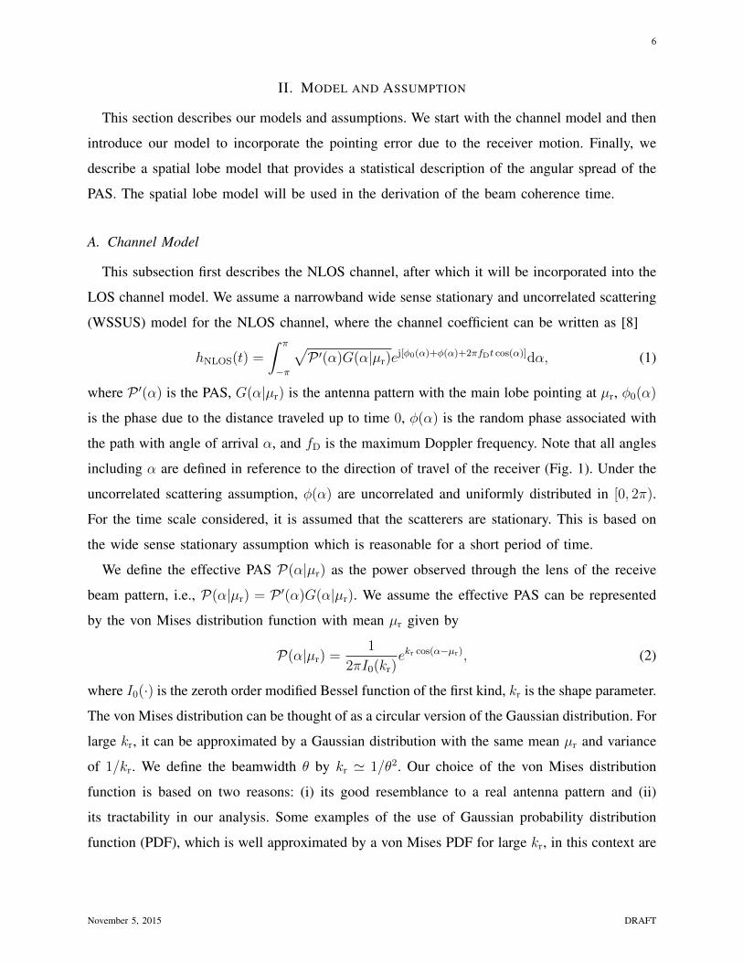
Our model for the NLOS case follows the one-ring model, where scatterers are distributed

on a ring of radius Dr as shown in Fig. 1. Assume the receiver is at point A at time t and it

moves with a speed v along the direction of travel to arrive at point B at time t + τ . The total

displacement from A to B is ∆d(τ) = vτ . When the receiver moves from A to B by ∆d(τ), the

receiver will see a different set of scatterers and the distances to the scatterers also change. We

assume that ∆d(τ)� Dr, so that the displancement ∆d(τ) has negligible effect on the path loss

and capture the receiver motion effect through the pointing error ∆µ(τ) as shown in Fig. 1. For

notational convenience, ∆µ,∆d are used instead of ∆µ(τ),∆d(τ). The relationship between ∆d

and ∆µ can be obtained from geometry as

tan(µr) =Dr sin(µr −∆µ)

Dr cos(µr −∆µ)−∆d

. (5)

Expanding the sine and cosine term in (5) and apply the small ∆µ approximation, i.e., sin ∆µ '

∆µ and cos ∆µ ' 1, then (5) becomessinµr

cosµr

' Dr sinµr −Dr∆µ cosµr

Dr cosµr +Dr∆µ sinµr −∆d

Dr∆µ sin2 µr −∆d sinµr ' −Dr∆µ cos2 µr.


8

∆d

Ring of scatterer

A B

Dr

Dr rcos(µ – )

µrµr

∆µ

Dr rsin(µ – )∆µ

∆µ

Direction of travel

Fig. 1. Receiver displacement and change in pointing angle for the NLOS case. When the receiver moves from A to B, if the

beam is not adaptive, then effectively the beam pointing angle changes.

Using the identity sin2 µr + cos2 µr = 1, a tractable approximation is obtained as

∆µ '∆d

Dr

sinµr. (6)

Since fD = v/λ, we have ∆d = vτ = fDλτ , where λ is the carrier wavelength. Substituting this

into (6) to get

∆µ 'fDτ

Dr,λ

sinµr, (7)

where Dr,λ = Dr/λ is the scattering radius normalized by the carrier wavelength λ.

The same reasoning can also be applied to the LOS case by replacing the scattering radius

Dr by the transmitter-receiver distance D. Let Dλ = D/λ and αLOS be the direction toward the

transmitter (in reference to the travel direction), then

∆LOSµ ' fDτ

Dλ

sin(αLOS). (8)

The approximate relation (7) and (8) will be incorporated with the channel model in the previous

section to derive an approximate channel temporal correlation function in Section III.

C. Channel Spatial Lobe Model

Here we explain the spatial lobe model that will be the basis for our definition of the

beam coherence time. Only the azimuthal plane is considered. This model provides a statistical

description of the angular spread of the PAS. A signal transmitted from the transmitter propagates

through different paths to arrive at the receiver. These multipaths arrive at different angles with


9

30

210

60

240

90

270

120

300

150

330

180 0

spatial lobe

#1

#3

#4

#2

lobe width

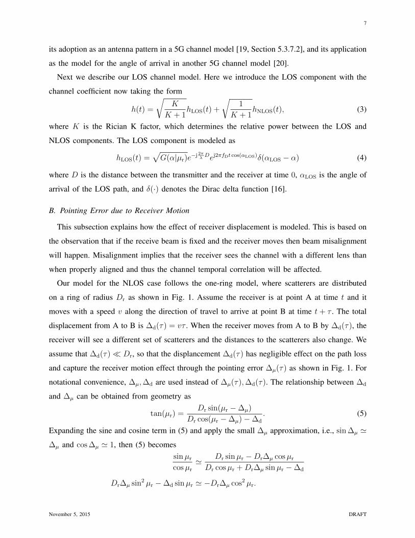
Fig. 2. An illustration of spatial lobes. This figure illustrates the pattern of the incoming power arriving at the receiver. The

incoming power has strong spatial dependence, and it can be observed here that there are four main directions, each of which

can be thought of as four clusters of scatterers. At each of these directions, there is spread forming a lobe, which is termed as

a spatial lobe. In this example, lobe #1 has the strongest power.

some concentrations at certain angles which create patterns as illustrated in Fig. 2, which are

called spatial lobes. Four spatial lobes are shown in Fig. 2. Each of them can be thought of as a

result of the power coming from the multipaths corresponding to a cluster of scatterers that have

similar angles of arrival. The number of spatial lobes depends on the environment and ranges

from 1-6 in an urban environment measurement at 28 GHz [21]. Beam alignment is the process

of finding the direction of the spatial lobe with the highest power, i.e., the lobe with the highest

peak (lobe #1 in Fig. 2). The lobe width determines the difficulty in aligning the beam. The

narrower the spatial lobe, the more difficult the alignment becomes, and the easier the beam

gets misaligned due to the receiver motion. Thus this lobe width plays a fundamental role in

defining the beam coherence time.

The lobe width β is modeled following the empirical model proposed in [21], which uses a

Gaussian distribution, i.e.,

β ∼ N (mAS, σ2AS). (9)

The mean mAS and the standard deviation σAS depend on the environment. The model in [21]

was based on measurements in urban area, where mAS = 34.8◦ and σAS = 25.7◦ were derived.


10

III. CHANNEL TEMPORAL CORRELATION FUNCTION

There are two possible definitions of the channel temporal correlation function. One is based

on the amplitude of the channel coefficients [9] and the channel correlation function is defined

by

R|h|(τ) =E [g(t)g(t+ τ)]− (E[g(t)])2

E[g(t)2]− (E[g(t)])2 , (10)

where g(t) = |h(t)|, and E[·] denotes the expectation operator. The other definition is based on

the complex channel coefficients themselves [10] and is defined as

Rh(τ) = E [h(t)h∗(t+ τ)] , (11)

where (·)∗ denotes complex conjugate. Most modern communication systems use coherent

detection, where both amplitude and phase are important. In that respect, the definition in (11) is

more natural and is the definition used in this study. It should be noted that when h(t) is Rayleigh

faded, the two definitions are in fact equivalent [22, Pages 47-51], in the sense that there is a

simple relationship between the two. In particular, it can be shown that R|h|(τ) = π4(4−π)

|Rh(τ)|2.

The channel model in (3) has both the LOS and NLOS components. For the LOS component,

hLOS(t) depends on the pointing direction, and proper normalization is needed to be consistent

with (11). We still define the correlation function for the LOS component RLOS(τ) based on the

product hLOS(t)h∗LOS(t+ τ) but now we introduce a normalization such that |RLOS(τ = 0)| = 1

and |RLOS(τ 6= 0)| < 1 in Section III-B. Along with this definition, the correlation function of

the channel is defined as

Rh(τ) =K

K + 1RLOS(τ) +

1

K + 1RNLOS(τ). (12)

In the followings, we derive the correlation function for the NLOS channel using (11) in Section

III-A and define the correlation function for the LOS in Section III-B that is consistent with the

definition in (11). In both cases, the effect of the receiver motion is taken into account.

A. NLOS Channel Correlation Function

Here we derive the correlation function between hNLOS(t) and hNLOS(t + τ) for the NLOS

channel. The channel coefficients at time t and t+ τ are given by,

hNLOS(t) =

∫ π

−π

√P(α|µr)e

j[φ0(α)+φ(α)+2πfDt cos(α)]dα, (13)

hNLOS(t+ τ) =

∫ π

−π

√P(α|µr + ∆µ)ej[φ0(α)+φ(α)+2πfD(t+τ) cos(α)]dα, (14)


11

where we have incorporated the pointing angular change due to the receiver motion in the peak

direction of the effective PAS, which is now µr + ∆µ instead of µr in (14). Plugging these into

the definition in (11),

RNLOS(τ) = E[∫ π

−π

∫ π

−π

√P(α1|µr)P(α2|µr + ∆µ)ej(φ0(α1)+φ(α1)−φ0(α2)−φ(α2)−2πfDτ cos(α2))dα1dα2

]=

∫ π

−π

∫ π

−π

√P(α1|µr)P(α2|µr + ∆µ)E[ej(φ(α1)−φ(α2))]ej(φ0(α1)−φ0(α2))e−j2πfDτ cos(α2)dα1dα2

=

∫ π

−π

√P(α|µr)P(α|µr + ∆µ)e−j2πfDτ cos(α)dα, (15)

where (15) follows from the uncorrelated scattering assumption. According to this assumption,

E[ej(φ(α1)−φ(α2))] = E[ejφ(α1)]E[e−jφ(α2)] = 0 for α1 6= α2 and E[ej(φ(α1)−φ(α2))] = 1 for α1 = α2,

where φ(α) is uniformly distributed in [0, 2π). Now substituting the von Mises PDF to get

RNLOS(τ) =1

2πI0(kr)

∫ π

−π

√ekr cos(α−µr)ekr cos(α−(µr+∆µ))e−j2πfDτ cos(α)dα (16)

=1

2πI0(kr)

∫ π

−πekr cos

(α−µr−∆µ

2

)cos

(∆µ2

)e−j2πfDτ cos(α)dα

=1

2πI0(kr)

∫ π

−πek′r cos(α−µ′)e−j2πfDτ cos(α)dα

=1

2πI0(kr)

∫ π

−πex′ cosα+y′ sinαdα

=I0(√x′2 + y′2)

I0(kr), (17)

where,

k′r = kr cos

(∆µ

2

)(18)

µ′ = µr +∆µ

2(19)

x′ = k′r cosµ′ − j2πfDτ (20)

y′ = k′r sinµ′. (21)

and we have used the formula∫ π−π e

a cos c+b sin cdc = 2πI0(√a2 + b2) [23, 3.338-4]. Despite the

simple form of (17), it is intractable for further analysis because the argument to the Bessel

function involves the cosine of ∆µ, which is also a function of τ . Fortunately, a more tractable

approximated form can be obtained for large kr, where the von Mises PDF can be approximated


12

by the Gaussian one with the variance of 1/kr and the same mean. With this approximation,

(16) becomes

RNLOS(τ) ' 1√2π/kr

∫ π

−πe−

kr4 ((α−µr)2+(α−(µr+∆µ))2)e−j2πfDτ cos(α)dα. (22)

The exponent can be simplified as follows.

(α− µr)2 + (α− (µr + ∆µ))2 =

(α−

(µ′ − ∆µ

2

))2

+

(α−

(µ′ +

∆µ

2

))2

= 2(α− µ′)2 +∆2µ

2. (23)

Substituting this into (22) and approximate µ′ ' µ, which is valid for small ∆µ, we have

RNLOS(τ) '∫ π

−π

1√2π/kr

ekr2

(α−µr)2

e−kr∆2

µ8 e−j2πfDτ cos(α)dα. (24)

To obtain a final closed form expression, the Gaussian PDF is approximated back to von Mises

one to get the following.

RNLOS(τ) ' e−kr∆2

µ8

2πI0(kr)

∫ π

−πekr cos(α−µr)e−j2πfDτ cos(α)dα

= e− krf

2Dτ

2 sin2 µr

8D2r,λ

I0(√x2 + y2)

I0(kr)(25)

where,

x = kr cosµr − j2πfDτ, (26)

y = kr sinµr. (27)

In this paper, we are interested in narrow receive beamwidths (i.e., kr large), and this approxima-

tion turns out to be decent enough for our purpose as will be shown in the numerical examples

at the end of this section. Note that in the approximation in (25), the effect of pointing error

due to the receiver motion is decoupled from the usual effect of Doppler spread to the channel.

B. LOS Channel Correlation Function

The correlation function for the LOS channel is defined as

RLOS(τ) =1

max{|hLOS(t)|2, |hLOS(t+ τ)|2}hLOS(t)h∗LOS(t+ τ), (28)


13

where the normalization is to ensure that |RLOS(τ)| ≤ 1. Substituting the channel in (4) we have

RLOS(τ) =

√G(αLOS|µr)G(αLOS|µr + ∆LOS

µ )

max{G(αLOS|µr), G(αLOS|µr + ∆LOSµ )}

× ej2πfDt[cos(αLOS)−cos(αLOS+∆LOSµ )]e−j2πfDτ cos(αLOS+∆LOS

µ ), (29)

where we have incorporated the receive beam pointing error due to the receiver motion over the

time period τ through ∆LOSµ as given in (8). Note that (29) depends on t and thus is not wide

sense stationary. In the case of small ∆LOSµ , it can be approximated as wide sense stationary as

the term ej2πfDt[cos(αLOS)−cos(αLOS+∆LOSµ )] ' 1. Note that |RLOS(τ)| = 1 only when ∆LOS

µ = 0.

If we assume that at time t the receive beam is pointing at αLOS, then G(αLOS|µr = αLOS) =

ekr/(2πI0(kr)) and G(αLOS|µr + ∆LOSµ ) = ekr cos(∆LOS

µ )/(2πI0(kr)) and we have

RLOS(τ) =

√ekr(cos(∆LOS

µ )−1)ej2πfDt[cos(αLOS)−cos(αLOS+∆LOSµ )]e−j2πfDτ cos(αLOS+∆LOS

µ ) (30)

' e12kr(cos(∆LOS

µ )−1)e−j2πfDτ cos(αLOS), (31)

where the approximation follows when ∆LOSµ is small, which typically is the case because the

transmitter-receiver distance D is large. Taking the absolute value of either (30) or (31) gives

|RLOS(τ)| = e12kr(cos(∆LOS

µ )−1). (32)

The expression in (32) means that the only factor affecting the channel correlation of the LOS

channel is the pointing error.

C. Numerical Verification of (25) and Effect of K Factor

First we will verify our approximation for the NLOS case in (25) by comparing it with the

exact expression given in (17) and the correlation computed from simulation. Then we provide

an example to show the effect of the K factor on the channel correlation. The derivation of

(25) is based on the assumption of small ∆µ, which depends on both the scattering radius Dr,λ

and the pointing direction µr. This assumption is most restrictive when µr approaches π/2 and

Dr,λ small. With this in mind, we set the transmitter-receiver distance D = 50 m, the receiver

speed v = 30 m/s, the carrier frequency fc = 60 GHz, the scattering radius Dr = 0.5 m (i.e.,

Dr,λ = 100). We compute the the case when µr = 10◦ and when µr = 80◦ to compare the

effect of µr. Note that there was no assumption on the receive beamwidth in the derivation, and

the accuracy of this approximation does not depend on the beamwidth. For this reason we fix


14

0 0.5 1 1.5 2 2.50

0.1

0.2

0.3

0.4

0.5

0.6

0.7

0.8

0.9

1

τ [ms]

Cha

nnel

Tim

e C

orre

latio

n |R

h(τ)|

exactapproximationsimulation

µr=80

µr=10

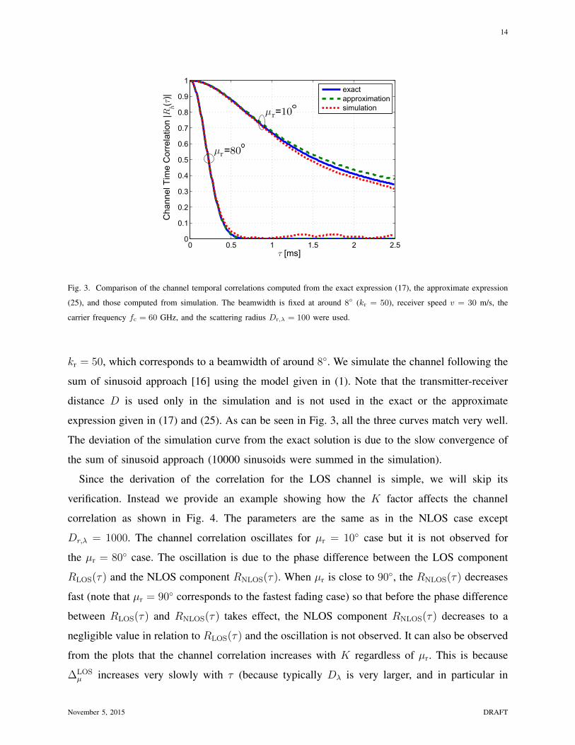
Fig. 3. Comparison of the channel temporal correlations computed from the exact expression (17), the approximate expression

(25), and those computed from simulation. The beamwidth is fixed at around 8◦ (kr = 50), receiver speed v = 30 m/s, the

carrier frequency fc = 60 GHz, and the scattering radius Dr,λ = 100 were used.

kr = 50, which corresponds to a beamwidth of around 8◦. We simulate the channel following the

sum of sinusoid approach [16] using the model given in (1). Note that the transmitter-receiver

distance D is used only in the simulation and is not used in the exact or the approximate

expression given in (17) and (25). As can be seen in Fig. 3, all the three curves match very well.

The deviation of the simulation curve from the exact solution is due to the slow convergence of

the sum of sinusoid approach (10000 sinusoids were summed in the simulation).

Since the derivation of the correlation for the LOS channel is simple, we will skip its

verification. Instead we provide an example showing how the K factor affects the channel

correlation as shown in Fig. 4. The parameters are the same as in the NLOS case except

Dr,λ = 1000. The channel correlation oscillates for µr = 10◦ case but it is not observed for

the µr = 80◦ case. The oscillation is due to the phase difference between the LOS component

RLOS(τ) and the NLOS component RNLOS(τ). When µr is close to 90◦, the RNLOS(τ) decreases

fast (note that µr = 90◦ corresponds to the fastest fading case) so that before the phase difference

between RLOS(τ) and RNLOS(τ) takes effect, the NLOS component RNLOS(τ) decreases to a

negligible value in relation to RLOS(τ) and the oscillation is not observed. It can also be observed

from the plots that the channel correlation increases with K regardless of µr. This is because

∆LOSµ increases very slowly with τ (because typically Dλ is very larger, and in particular in


15

0 5 10 15 20 250

0.2

0.4

0.6

0.8

1|R

h(τ

)|

τ [ms]

increasing K

(a) When µr = 10◦

0 0.5 1 1.5 2 2.5 30

0.2

0.4

0.6

0.8

1

|Rh(τ

)|

τ [ms]

increasing K

(b) When µr = 80◦

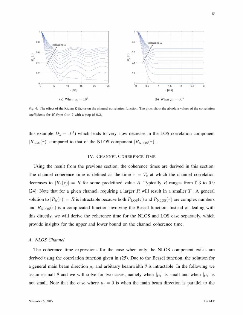
Fig. 4. The effect of the Rician K factor on the channel correlation function. The plots show the absolute values of the correlation

coefficients for K from 0 to 2 with a step of 0.2.

this example Dλ = 104) which leads to very slow decrease in the LOS correlation component

|RLOS(τ)| compared to that of the NLOS component |RNLOS(τ)|.

IV. CHANNEL COHERENCE TIME

Using the result from the previous section, the coherence times are derived in this section.

The channel coherence time is defined as the time τ = Tc at which the channel correlation

decreases to |Rh(τ)| = R for some predefined value R. Typically R ranges from 0.3 to 0.9

[24]. Note that for a given channel, requiring a larger R will result in a smaller Tc. A general

solution to |Rh(τ)| = R is intractable because both RLOS(τ) and RNLOS(τ) are complex numbers

and RNLOS(τ) is a complicated function involving the Bessel function. Instead of dealing with

this directly, we will derive the coherence time for the NLOS and LOS case separately, which

provide insights for the upper and lower bound on the channel coherence time.

A. NLOS Channel

The coherence time expressions for the case when only the NLOS component exists are

derived using the correlation function given in (25). Due to the Bessel function, the solution for

a general main beam direction µr and arbitrary beamwidth θ is intractable. In the following we

assume small θ and we will solve for two cases, namely when |µr| is small and when |µr| is

not small. Note that the case where µr = 0 is when the main beam direction is parallel to the


16

direction of travel resulting the slowest fading case, while |µr| = π/2 is when the main beam

direction is perpendicular to the direction of travel and the receiver will experience the fastest

fading [9]. For most cases, our approximation is valid for beamwidth θ up to around 20◦. This is

not a big limitation because most likely mmWave systems will use narrow beams. For example,

a prototype system developped by Samsung Electronics uses an array with 10◦ beamwidth in

azimuth [25] and long range automotive radars use beamwidth on the order of a few degrees

[26].

1) When |µr| is small: For small µr, we approximate x ' kr−j2πfDτ and y ' 0, where x and

y are defined in (26) and (27), respectively. Note that the accuracy of this approximation depends

on both kr and µr. When µr is small, y ' krµr ' µr/θ2 and thus roughly the approximation

works for θ >√µr. Assuming θ is in this range we can apply the approximation to get

Rh(τ) ' e− krf

2Dτ

2 sin2 µr

8D2r,λ

I0(kr − j2πfDτ)

I0(kr)(33)

' e− krf

2Dτ

2 sin2 µr

8D2r,λ

e−j2πfDτ√1− j2πfDτ/kr

. (34)

The last step follows by applying the asymptotic approximation of the Bessel function [27]

I0(z) ' ez√2πz

, (35)

which holds for |z| large. Taking the absolute value to get

|Rh(τ)| ' e− krf

2Dτ

2 sin2 µr

8D2r,λ

1

|√

1− j2πfDτ/kr|(36)

= e− krf

2Dτ

2 sin2 µr

8D2r,λ

1

(1 + (2πfDτ/kr)2)1/4. (37)

Following the definition |Rh(Tc)| = R, we can solve for Tc as follows.

1 + (2πfDTc/kr)2 =

1

R4e− krf

2DT

2c sin2 µr

2D2r,λ (38)

' 1

R4

(1− krf

2DT

2c sin2 µr

2D2r,λ

)(39)

⇒ Tc =

√√√√ 1/R4 − 1

(2πfD/kr)2 +krf2

D sin2 µr

2D2r,λR

4

(40)


17

where we have used the approximation ez ' 1 + z to eliminate the exponential term. For small

beamwidth we have kr ' 1/θ2 and thus in terms of beamwidth we have

Tc(θ) =

√√√√ 1/R4 − 1

(2πfD)2θ4 + 12θ2R4

(fD sinµr

Dr,λ

)2 . (41)

When Dr,λ →∞, i.e., ignoring the pointing angular change due to the receiver movement, the

coherence time simplifies to

Tc(θ) =

√1/R4 − 1

2πfDθ2. (42)

We can see that in this case the coherence time is inversely proportional to θ2.

2) When |µr| is not small: The approach here is different from the previous case. First we

compute the argument of the Bessel function, and then we apply asymptotic approximation (35).

Taking the log of the obtained equation, we get a polynomial equation of τ . Exact solution is not

trivial, but considering the range of values of the parameters, higher order terms are negligible

and we can approximately solve a quadratic equation instead.

Defining c + jd =√x2 + y2 where x and y are given in (26) and (27) respectively. With

simple algebra, c and d can be derived as

c =

√√a2 + b2 + a

2, d =

b

2c, (43)

where a = k2r − (2πfD)2τ 2 and b = −4πfDkr cos(µr)τ . Substitute c and d above into (25), apply

the asymptotic approximation (35), and finally take the absolute value we have

R = e− krf

2Dτ

2 sin2 µr

8D2r,λ

ec−kr

(1 + (b/2k2r )2)1/4

. (44)

For large kr, the denominator takes values close to one, and we approximate (1+(b/2k2r )2)1/4 ' 1.

Taking the log on both sides and rearranging we have

kr + logR +krf

2Dτ

2 sin2 µr

8D2r,λ

=

√√a2 + b2 + a

2.

Now taking the square of both sides and ignore the τ 4 term to get

2(kr + logR)2 + 4(kr + log(R))krf

2Dτ

2 sin2 µr

8D2r,λ

− a =√a2 + b2.


18

Once again taking the square of both sides to get rid of the square root, and neglect the higher

order terms with respect to τ . Then substitute a and b we obtain (45), from which the approximate

channel coherence time expression (46) can be readily derived.

4(kr + logR)4 − 4k2r (kr + logR)2 +

[16(kr + logR)3 − 8k2

r (kr + logR)]krf

2D sin2 µr

8D2r,λ

τ 2

+4(kr + logR)2(2πfD)2τ 2 = (4πfDkr cosµr)2τ 2 (45)

T 2c =

k2r − (kr + logR)2[

4(kr + logR)− 2 k2r

kr+logR

]krf2

D sin2 µr

8D2r,λ

+ (2πfD)2 − (4πfDkr cosµr)2

(kr+logR)2

. (46)

Note that for a fixed µr the denominator in (46) can be negative leading to invalid solution.

The range of valid solution increases with µr as will be shown in our numerical example. As

evident from Fig. 6, if µr is not too small, our result covers most of the beamwidths of interest

for mmWave systems.

For the special case when µr = 90◦, which is the fastest fading case, (46) can be simplified

by approximating 4(kr + logR)− 2 k2r

kr+logR' 2(kr + logR), which is valid for large kr. Finally

using the relationship kr = 1θ2 , the worst case channel coherence time can be expressed as

Tc(θ) =

√√√√√ 1− (1 + θ2 logR)2

14

(1 + θ2 logR)(fD sinµr

Dr,λ

)2

+ (2πfD)2θ4

. (47)

When Dr,λ →∞, this simplifies to

Tc(θ) =1

2πfD

√1

θ2log

1

R2− (logR)2. (48)

Using the approximation√

1 + z ' 1 + 1z

for small z, it can be shown that Tc(θ) increases on

the order of 1/θ for small θ at the pointing angle µr = 90◦.

B. LOS Channel

When the LOS dominates, K/(K + 1)→ 1 and Rh(τ) ' RLOS(τ). Thus we have

|Rh(τ)| = e12kr(cos(∆LOS

µ )−1). (49)

Substituting (8) for ∆LOSµ and using the definition |Rh(Tc)| = R, the above equation can be

easily solved to get

Tc(θ) =Dλ

fD sin(αLOS)cos−1

(2

kr

logR + 1

)(50)

=Dλ

fD sin(αLOS)cos−1

(2θ2 logR + 1

). (51)


19

0 5 10 15 20 25 3010−4

10−3

10−2

10−1

Beamwidth θ [deg]

Coh

eren

ce T

ime

T c [s

]ExactApproximationNo angular difference

(a) µr = 1◦

0 5 10 15 20 25 3010−4

10−3

10−2

10−1

Beamwidth θ [deg]

Coh

eren

ce T

ime

T c [s

]

ExactApproximationNo angular difference

(b) µr = 5◦

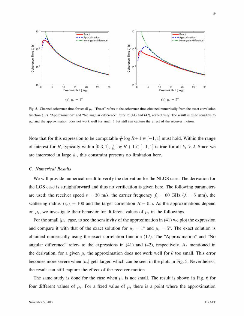
Fig. 5. Channel coherence time for small µr. “Exact” refers to the coherence time obtained numerically from the exact correlation

function (17). “Approximation” and “No angular difference” refer to (41) and (42), respectively. The result is quite sensitive to

µr, and the approximation does not work well for small θ but still can capture the effect of the receiver motion.

Note that for this expression to be computable 2kr

logR+1 ∈ [−1, 1] must hold. Within the range

of interest for R, typically within [0.3, 1], 2kr

logR+ 1 ∈ [−1, 1] is true for all kr > 2. Since we

are interested in large kr, this constraint presents no limitation here.

C. Numerical Results

We will provide numerical result to verify the derivation for the NLOS case. The derivation for

the LOS case is straightforward and thus no verification is given here. The following parameters

are used: the receiver speed v = 30 m/s, the carrier frequency fc = 60 GHz (λ = 5 mm), the

scattering radius Dr,λ = 100 and the target correlation R = 0.5. As the approximations depend

on µr, we investigate their behavior for different values of µr in the followings.

For the small |µr| case, to see the sensitivity of the approximation in (41) we plot the expression

and compare it with that of the exact solution for µr = 1◦ and µr = 5◦. The exact solution is

obtained numerically using the exact correlation function (17). The “Approximation” and “No

angular difference” refers to the expressions in (41) and (42), respectively. As mentioned in

the derivation, for a given µr the approximation does not work well for θ too small. This error

becomes more severe when |µr| gets larger, which can be seen in the plots in Fig. 5. Nevertheless,

the result can still capture the effect of the receiver motion.

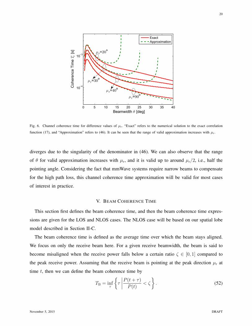
The same study is done for the case when µr is not small. The result is shown in Fig. 6 for

four different values of µr. For a fixed value of µr there is a point where the approximation


20

0 5 10 15 20 25 30 35 40

10−4

10−3

Beamwidth θ [deg]

Coh

eren

ce T

ime

T c [s

]

ExactApproximation

µr=20

µr=30

µr=40

µr=90

Fig. 6. Channel coherence time for difference values of µr. “Exact” refers to the numerical solution to the exact correlation

function (17), and “Approximation” refers to (46). It can be seen that the range of valid approximation increases with µr.

diverges due to the singularity of the denominator in (46). We can also observe that the range

of θ for valid approximation increases with µr, and it is valid up to around µr/2, i.e., half the

pointing angle. Considering the fact that mmWave systems require narrow beams to compensate

for the high path loss, this channel coherence time approximation will be valid for most cases

of interest in practice.

V. BEAM COHERENCE TIME

This section first defines the beam coherence time, and then the beam coherence time expres-

sions are given for the LOS and NLOS cases. The NLOS case will be based on our spatial lobe

model described in Section II-C.

The beam coherence time is defined as the average time over which the beam stays aligned.

We focus on only the receive beam here. For a given receive beamwidth, the beam is said to

become misaligned when the receive power falls below a certain ratio ζ ∈ [0, 1] compared to

the peak receive power. Assuming that the receive beam is pointing at the peak direction µr at

time t, then we can define the beam coherence time by

TB = infτ

{τ

∣∣∣∣P (t+ τ)

P (t)< ζ

}. (52)


21

Note that the power decrease here is due to the pointing error ∆µ(τ) as defined in Section II-B.

Using this definition, we derive the beam coherence times in the followings.

A. LOS Case

The pointing angular change ∆LOSµ is given in (8). Let the beam pattern be represented by the

von Mises distribution as earlier, the receive power is proportional to the receive beam pattern.

In particular, P (t) ∝ G(µr|µr) and P (t+ τ) ∝ G(µr|µr + ∆LOSµ ). At τ = TB,

ζ =G(µr|µr + ∆LOS

µ )

G(µr|µr)(53)

= ekr(cos(∆LOSµ )−1). (54)

Substituting ∆LOSµ from (8) the above equation can be easily solved to get

TB(θ) =Dλ

fD sinµr

cos−1(θ2 log ζ + 1

), (55)

where we have used kr = 1/θ2 in the above expression. Note that this expression is closely

related to the expression for the channel coherence time for the LOS case.

B. NLOS Case

First we need to find the pointing angular change due to the receiver motion. In the NLOS

case, the incoming power is the result of the reflection from the scatterers. Following our one-ring

scatter model, the pointing angular change is given by (7).

Now we need to compute the receive power and use the expression to solve for TB. Assuming

the spatial lobes are also represented by the von Mises distribution with lobe width given by β,

which is defined in (9), or by the concentration parameter κr = 1/β2, and has peak at µr. This

is the PAS P ′(α|µr) before applying the receive beam pattern. At time t assume that the receive

beam is pointing at the peak of P ′(α|µr), i.e., using the beam pattern G(α|µr). At time t + τ ,

the beam pattern now changes to G(α|µr + ∆µ) if no realignment is done. The receive power

at a pointing angle µr + ∆µ is given by

P (t+ τ) =

∫ 2π

0

P ′(α|µr)G(α|µr + ∆µ)dα. (56)


22

Note that for large kr the von Mises PDF in (2) approaches the Gaussian PDF [28, Ch. 45]. Also

note that for large kr, i.e., small variance, the distribution falls off fast and tails at both sides

beyond 0 and 2π have little weight. These observations lead to the following approximation:

P (t+ τ) '∫ ∞−∞

1√2πβ2

e− (α−µr)2

2β21√

2πθ2e−

(α−µr−∆µ)2

2θ2 dα

=

∫ ∞−∞

1√2πβ2

e− (u)2

2β21√

2πθ2e−

(∆µ−u)2

2θ2 du. (57)

Applying a change of variable u = α− µr, µr can be eliminated from the first expression. The

expression (57) is just a convolution between two Gaussian PDFs, which is well-known to result

in another Gaussian PDF with mean ∆µ and variance β2 + θ2 [29]. That is,

P (t+ τ) ' 1√2π(β2 + θ2)

e− ∆2

µ

2(β2+θ2) , (58)

which does not depend on µr. This makes sense because in the current setting it is assumed

that at time t the receive beam is aligned to µr and P (t + τ) is determined solely from the

misalignment that happens at time t + τ . This misalignment is captured by pointing error due

to the receiver motion ∆µ, which is a function of τ . We can solve for TB directly from (58);

however, by approximating (58) by a von Mises distribution function, the resulting TB is of the

same form for both the LOS and NLOS cases. Doing this approximation, (58) becomes

P (t+ τ) ' 1

2πI0(1/(β2 + θ2))e

cos(∆µ)

β2+θ2 . (59)

With the same steps used in the derivation of the beam coherence time for the LOS case, we

get the expression for the NLOS case as

TB(θ|β) =Dr,λ

fD sinµr

cos−1((β2 + θ2) log ζ + 1

). (60)

Note that β is a random variable and is modeled by the Gaussian distribution in (9). Thus to

get the beam coherence time we need to average over β,

TB(θ) = Eβ[TB(θ|β)]. (61)

where Eβ[·] denotes the statistical expectation over β. The difference to the LOS case is that

now TB depends on the channel through the spatial lobe angular spread parameter β.


23

0 5 10 15 20 25 300

1

2

3

4

5

6

7

Beamwidth θ [deg]

Beam

coh

eren

ce ti

me

T B [s

]µr=10°

µr=80°

(a) Beam coherence time for LOS case

0 5 10 15 20 25 300

0.1

0.2

0.3

0.4

0.5

0.6

0.7

0.8

Beamwidth θ [deg]

Beam

coh

eren

ce ti

me

T B [s

]

mean AoA=10°

mean AoA=80°

(b) Beam coherence time for NLOS case

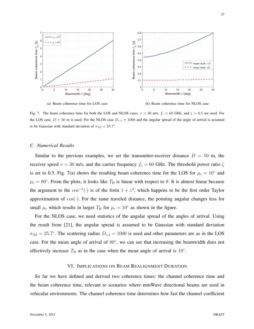
Fig. 7. The beam coherence time for both the LOS and NLOS cases. v = 30 m/s, fc = 60 GHz, and ζ = 0.5 are used. For

the LOS case, D = 50 m is used. For the NLOS case Dr,λ = 1000 and the angular spread of the angle of arrival is assumed

to be Gaussian with standard deviation of σAS = 25.7◦

C. Numerical Results

Similar to the previous examples, we set the transmitter-receiver distance D = 50 m, the

receiver speed v = 30 m/s, and the carrier frequency fc = 60 GHz. The threshold power ratio ζ

is set to 0.5. Fig. 7(a) shows the resulting beam coherence time for the LOS for µr = 10◦ and

µr = 80◦. From the plots, it looks like TB is linear with respect to θ. It is almost linear because

the argument to the cos−1(·) is of the form 1 + z2, which happens to be the first order Taylor

approximation of cos(·). For the same traveled distance, the pointing angular changes less for

small µr which results in larger TB for µr = 10◦ as shown in the figure.

For the NLOS case, we need statistics of the angular spread of the angles of arrival. Using

the result from [21], the angular spread is assumed to be Gaussian with standard deviation

σAS = 25.7◦. The scattering radius Dr,λ = 1000 is used and other parameters are as in the LOS

case. For the mean angle of arrival of 80◦, we can see that increasing the beamwidth does not

effectively increase TB as in the case when the mean angle of arrival is 10◦.

VI. IMPLICATIONS ON BEAM REALIGNMENT DURATION

So far we have defined and derived two coherence times: the channel coherence time and

the beam coherence time, relevant to scenarios where mmWave directional beams are used in

vehicular environments. The channel coherence time determines how fast the channel coefficient


24

changes in time, and thus can be used in deciding the packet length and determining the overhead

for channel estimation. We explore some implications of on the choice of beamwidth in this

section. We argue in Section VI-B that, to maximize the performance, beam realignment can be

done in every beam coherence time not in every channel coherence time.

A. Lower Bound on Mutual Information

Consider the following signal model.

y[i] = h[i]s[i] + n[i], i = 1, 2, . . . , k (62)

where y[i] is the receive signal, h[i] is the channel, s[i] is the transmitted signal, n[i] is the

additive white Gaussian noise (AWGN), and k is the packet length measured in the number of

samples. It is assumed that the channel h[i] is normalized such that its variance is σ2h = 1 for all

i. A simple autoregressive temporal correlation function is used to describe the time-variation

of the channel in discrete-time as

h[i] = αh[i− 1] + ξ[i− 1], (63)

where α is the correlation coefficient and is given by

α = Rh(νT ) (64)

with the symbol duration T , ξ[i] is the innovation term with variance σ2ξ = (1 − |Rh(νT )|2),

and Rh(·) is the channel temporal correlation function derived in Section III. For decoding, the

channel has to be estimated, and the estimation is affected from both the thermal noise and the

channel time-variation.

If the estimator does not have knowledge of the statistics of ξ[i] (which typically is the case),

then a natural assumption is that ξ[i] is Gaussian. Because (63) is a Gauss-Markov channel

model, following the logic used in [24], the Kalman filter provides the maximum-likelihood

estimate (and also the minimum mean squared error estimate) [30]. Suppose the channel is

estimated with the help of pilot symbols equally spaced in every ν samples. The receive pilot

signal vector can then be written as vbk/νc, where b·c denotes the floor function and ak denotes

a vector of length k. Applying the Kalman filter based on this pilot vector vbk/νc, the variance


25

of the channel estimation error at the `-th pilot ψ` is given by the following recursive relations

[24]

1

ψ1

=1

σ2h + σ2

ξ

+σ2v

σ2n

(65)

1

ψ`+1

=1

α2ψ` + σ2ξ

+σ2v

σ2n

, (66)

where σ2h is the channel variance, σ2

v is the pilot signal power assumed to be the same for all

pilot symbols, and σ2n is the noise power. To explicitly express the channel estimation error, the

channel is decomposed as

h[i] = h[i] + h[i], (67)

where h[i] is the known part and h[i] is the estimation error. The variance of the known part

h[i] can be written as

σ2h[i] = σ2

h − σ2h[i]. (68)

This notation is used in the derivation of the lower bound below. Note that the estimation error

variances given in (65) and (66) are at the sampling points corresponding to the pilots. When they

are used to decode the data part, the channel time variation will further degrade the estimation

accuracy. This increase in estimation error is determined from the channel correlation function

and the total estimation error variance at a given sampling point can be written as

σ2h[i] = ψbi/νc + (1− |Rh((i− bi/νcν)T )|2). (69)

For very long sequence of signal, e.g., when k →∞, the error variance from the Kalman filter

converges to some value ψ (i.e., does not depend on the pilot index) given by [24]

ψ =|Rh(νT )|2 − 1− SNRvGa(θ)σ2

ξ

2SNRvGa(θ)|Rh(νT )|2

+

√(|Rh(νT )|2 − 1− SNRvGa(θ)σ2

ξ )2 + 4SNR2

vGa(θ)σ2ξ |Rh(νT )|2

2SNRvGa(θ)|Rh(νT )|2. (70)

where SNRv = σ2v/σ

2n is the SNR of the pilot symbol excluding the antenna gain. Ga(θ) is the

antenna gain compared to omnidirectional antenna and is given by

Ga(θ) =G(µr|µr)

1/(2π)=

e1/θ2

I0(1/θ2)(71)

where 1/(2π) in the denominator is the gain of the omnidirectional antenna, and G(µr|µr) is

the peak of the antenna pattern with the main beam pointing at µr. G(α|µr) is assumed to have


26

the shape of the von Mises PDF. Note that we use the peak of the antenna pattern here because

the time scale of a packet is small and there will be negligible change in the pointing direction

within one packet.

Now consider the mutual information for only the i-th sample with channel estimate with

error given in (70). The worst case that the error h[i] can have is to act as AWGN [24]. In that

case, the mutual information can be lower bounded by

I(s[i]; y[i]|vbi/νc) ≥ ln

(1 +

σ2h[i]σ2

s

σ2hσ2s + σ2

n

). (72)

Using (72), and assuming the estimator does not use the decoded data for channel estimation

and only use the pilot vbi/νc then it can be shown that [24]

I(sk; (yk,vbk/νc)) ≥∑i≤k

I(s[i]; y[i]|vbi/νc). (73)

Plugging in the result so far, a lower bound for the mutual information can be written as

I(sk; (yk,vbk/νc)) ≥∑i≤k

ln

(1 +

(|Rh((i− bi/νcν)T )|2 − ψbi/νc)SNRsGa(θ)

(ψbi/νc + (1− |Rh((i− bi/νcν)T )|2))SNRsGa(θ) + 1

)(74)

where SNRs = σ2s /σ

2n is the SNR of the data part excluding the antenna gain. Further assume

k →∞ then ψbi/kc → ψ, and we have

limk→∞

1

kI(sk; (yk,vbk/νc)) ≥

1

ν

ν∑i=2

ln

(1 +

(|Rh(iT )|2 − ψ)SNRsGa(θ)

(ψ + (1− |Rh(iT )|2))SNRsGa(θ) + 1

)(75)

= Ilow(θ, SNRs, ν). (76)

At high SNR or when beamwidth θ is small (i.e., the antenna gain Ga(θ) is large), then

Ilow(θ, SNRs, ν) ' 1

ν

ν∑i=2

ln

(1 +

|Rh(iT )|2 − ψψ + (1− |Rh(iT )|2)

)(77)

which implies that the loss due to the channel time-variation acts in the same way as the

interference and it cannot be mitigated by increasing the transmit power.

Fig. 8(a) shows plots of the lower bound on the mutual information for different values of

the coherence bandwidth against the pilot spacing ν (Note that ν determines the overhead for

channel estimation. The larger ν is the lower the overhead.) In this example, SNRs = SNRv = 0

dB, beamwidth is fixed at θ = 10◦, and µr = 0◦ are used. We can see that in all these cases,

there is an optimal ν that maximizes the lower bound. As the coherence bandwidth increases

(thus T = 1/Bc decreases), the time variation measured in the number of samples increases and

the optimal ν increases.


27

0

0.5

1

1.5

2

2.5

3

3.5

4

10 100 1000Pilot spacing ν

I low

[bps/

Hz]

Bc =0.1 MHz

Bc =1 MHz

Bc =10 MHz

Bc =100 MHz

(a) Ilow for different coherence bandwidths

10 100 10001.5

2

2.5

3

3.5

4

I low

[bps/

Hz]

Pilot spacing ν

µr=0°

µr=30°

µr=60°

µr=90°

(b) Ilow for different µr

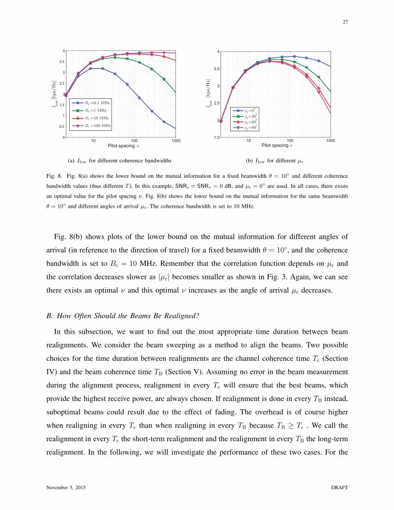
Fig. 8. Fig. 8(a) shows the lower bound on the mutual information for a fixed beamwidth θ = 10◦ and different coherence

bandwidth values (thus different T ). In this example, SNRs = SNRv = 0 dB, and µr = 0◦ are used. In all cases, there exists

an optimal value for the pilot spacing ν. Fig. 8(b) shows the lower bound on the mutual information for the same beamwidth

θ = 10◦ and different angles of arrival µr. The coherence bandwidth is set to 10 MHz.

Fig. 8(b) shows plots of the lower bound on the mutual information for different angles of

arrival (in reference to the direction of travel) for a fixed beamwidth θ = 10◦, and the coherence

bandwidth is set to Bc = 10 MHz. Remember that the correlation function depends on µr and

the correlation decreases slower as |µr| becomes smaller as shown in Fig. 3. Again, we can see

there exists an optimal ν and this optimal ν increases as the angle of arrival µr decreases.

B. How Often Should the Beams Be Realigned?

In this subsection, we want to find out the most appropriate time duration between beam

realignments. We consider the beam sweeping as a method to align the beams. Two possible

choices for the time duration between realignments are the channel coherence time Tc (Section

IV) and the beam coherence time TB (Section V). Assuming no error in the beam measurement

during the alignment process, realignment in every Tc will ensure that the best beams, which

provide the highest receive power, are always chosen. If realignment is done in every TB instead,

suboptimal beams could result due to the effect of fading. The overhead is of course higher

when realigning in every Tc than when realigning in every TB because TB ≥ Tc . We call the

realignment in every Tc the short-term realignment and the realignment in every TB the long-term

realignment. In the following, we will investigate the performance of these two cases. For the


28

LOS channel, Tc and TB are of comparable values (see (51) and (55)), and there is not much

difference between the two. Therefore we study the NLOS case only in the followings.

For clarity, we consider a channel with only two paths. Denote ∆ ≥ 1 the path loss ratio

between the first and second path, PLi for i = {1, 2} the path losses of the two paths, then

PL1 = PL2 ∆, (78)

where we have assumed without loss of generality that the first path has higher average receive

power. Let gi = |hi|2 and Pi where i = {1, 2} be the fading and the instantaneous receive power,

respectively, then we have

Pi = giPLi. (79)

Note that our channel model in (1) corresponds to the fading coefficient and no path loss was

incorporated.

The beam sweeping will select a beam following the rule i? = arg maxi Pi, explicitly

i? =

1 if g1 ≥ g2/∆

2 if g1 < g2/∆. (80)

Let fg(g) be the PDF of gi, then the beam sweeping will output 1 and 2 with probabilities

P{i? = 1} =

∫ ∞0

∫ ∞g2/∆

fg(g1)dg1fg(g2)dg2, (81)

P{i? = 2} =

∫ ∞0

∫ g2/∆

0

fg(g1)dg1fg(g2)dg2, (82)

respectively.

To have tractable analysis, we assume the fading is Rayleigh so that gi follows an exponential

distribution with unit mean. When realigning in every Tc, the path yielding the highest power

is always chosen, so that the receive power follows the distribution of max{P1, P2}. The SNR

is proportional to the received power, and the SNR PDF can be derived as

fshort(γ) =1

γ1

e−γ/γ1 +1

γ2

e−γ/γ2 −(

1

γ1

+1

γ2

)e−(1/γ1+1/γ2)γ, (83)

where γi = PiPn

is the average SNR of the i-th path and Pn is the noise power. When realigning in

every TB, the beam sweeping is performed at the beginning and the selected beam will be used

until the next realignment. Note that TB � Tc for the NLOS channels (see numerical examples in

Section IV and V). The fading coefficient becomes uncorrelated after Tc, thus the beam selected


29

at the beginning could result in suboptimal receive power. Depending on the result of the beam

sweeping the channel experienced here follows either P1 or P2. The SNR in this case follows

flong(γ) =1

γie−1/γi . (84)

So far we have derived the distribution of the SNR for the short- and long-term realignment.

Now we will discuss the overhead of the two realignment durations. The time needed for beam

sweeping is the same for both the short- and long-term realignments. Denoting this time duration

by Tsw, then the temporal efficiencies of the short- and long-term realignments are

ηshort(θ) =Tc(θ)− Tsw(θ)

Tc(θ)(85)

ηlong(θ) =TB(θ)− Tsw(θ)

TB(θ). (86)

Note that all these are functions of the beamwidth θ.

Finally, the loss due to the channel time-variation, the temporal efficiency, and the bound on

the mutual information are all considered for the overall performance metric, i.e.,

Cshort(θ) = ηshort(θ)Eshort [Ilow(θ, γshort, ν)] (87)

Clong(θ) = ηlong(θ)Elong [Ilow(θ, γlong, ν)] (88)

= ηlong(θ) (P{i? = 1}Eγ1 [Ilow(θ, γ1, ν)] + P{i? = 2}Eγ2 [Ilow(θ, γ2, ν)]) (89)

where Ilow(θ, γ, ν) is the lower bound derived in (76) in the previous subsection.

Now we provide a numerical example comparing the spectral efficiencies in (87) and (88)

when realignment duration is set to Tc versus TB. To make the comparison meaningful, the pilot

spacing ν should be optimized for all θ. Fig. 9 shows plots for different θ for both the short-

and long-term realignment. As can be observed from the plots, the sensitivity to ν is small near

the optimal ν, and in this case ν = 64 is optimal or has negligible loss for all the range of

beamwidth up to 30◦. Based on this we set ν = 64, and compute the spectral efficiencies as

a function of θ. For the beam sweeping, we consider a basic approach adopted in the IEEE

802.15.3c [31] which is based on hierarchical beam codebook. Let ` the number of levels in the

codebook, and the i-level has Li beams. In this approach, at each level all the beam combination

pairs are tested, so the overhead of beam training is L2iTTRN for the search at the i-th level. TTRN

is the duration needed for one beam measurement. Thus the 802.15.3c method has overhead of

T3c = TTRN

∑1/`i=1 L

2i . It can be shown that the optimum Li that minimize the number of beam


30

10 100 10000

1

2

3

4

5

6

7

Pilot spacing

Ave

rage

I low [b

ps/H

z]

Short−termLong−term

θ=1◦ θ=10◦

θ=30◦

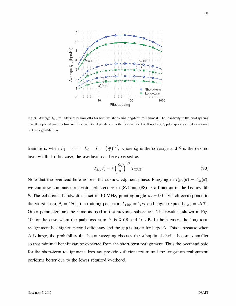
Fig. 9. Average Ilow for different beamwidths for both the short- and long-term realignment. The sensitivity to the pilot spacing

near the optimal point is low and there is little dependence on the beamwidth. For θ up to 30◦, pilot spacing of 64 is optimal

or has negligible loss.

training is when L1 = · · · = L` = L =(θ0θ

)1/`, where θ0 is the coverage and θ is the desired

beamwidth. In this case, the overhead can be expressed as

T3c(θ) = `

(θ0

θ

)2/`

TTRN. (90)

Note that the overhead here ignores the acknowledgment phase. Plugging in TSW(θ) = T3c(θ),

we can now compute the spectral efficiencies in (87) and (88) as a function of the beamwidth

θ. The coherence bandwidth is set to 10 MHz, pointing angle µr = 90◦ (which corresponds to

the worst case), θ0 = 180◦, the training per beam TTRN = 1µs, and angular spread σAS = 25.7◦.

Other parameters are the same as used in the previous subsection. The result is shown in Fig.

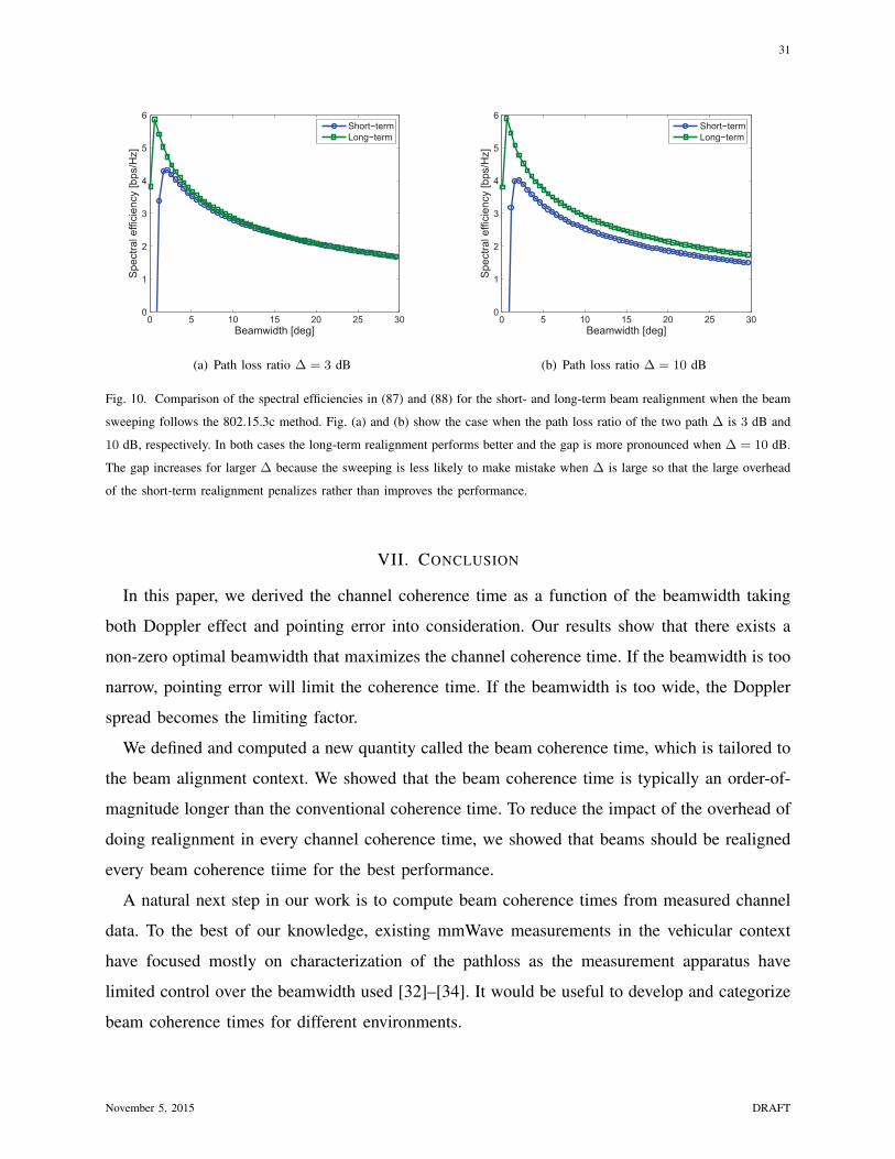
10 for the case when the path loss ratio ∆ is 3 dB and 10 dB. In both cases, the long-term

realignment has higher spectral efficiency and the gap is larger for large ∆. This is because when

∆ is large, the probability that beam sweeping chooses the suboptimal choice becomes smaller

so that minimal benefit can be expected from the short-term realignment. Thus the overhead paid

for the short-term realignment does not provide sufficient return and the long-term realignment

performs better due to the lower required overhead.


31

0 5 10 15 20 25 300

1

2

3

4

5

6

Beamwidth [deg]

Spe

ctra

l effi

cien

cy [b

ps/H

z]


(a) Path loss ratio ∆ = 3 dB

0 5 10 15 20 25 300

1

2

3

4

5

6

Beamwidth [deg]

Spe

ctra

l effi

cien

cy [b

ps/H

z]


(b) Path loss ratio ∆ = 10 dB

Fig. 10. Comparison of the spectral efficiencies in (87) and (88) for the short- and long-term beam realignment when the beam

sweeping follows the 802.15.3c method. Fig. (a) and (b) show the case when the path loss ratio of the two path ∆ is 3 dB and

10 dB, respectively. In both cases the long-term realignment performs better and the gap is more pronounced when ∆ = 10 dB.

The gap increases for larger ∆ because the sweeping is less likely to make mistake when ∆ is large so that the large overhead

of the short-term realignment penalizes rather than improves the performance.

VII. CONCLUSION

In this paper, we derived the channel coherence time as a function of the beamwidth taking

both Doppler effect and pointing error into consideration. Our results show that there exists a

non-zero optimal beamwidth that maximizes the channel coherence time. If the beamwidth is too

narrow, pointing error will limit the coherence time. If the beamwidth is too wide, the Doppler

spread becomes the limiting factor.

We defined and computed a new quantity called the beam coherence time, which is tailored to

the beam alignment context. We showed that the beam coherence time is typically an order-of-

magnitude longer than the conventional coherence time. To reduce the impact of the overhead of

doing realignment in every channel coherence time, we showed that beams should be realigned

every beam coherence tiime for the best performance.

A natural next step in our work is to compute beam coherence times from measured channel

data. To the best of our knowledge, existing mmWave measurements in the vehicular context

have focused mostly on characterization of the pathloss as the measurement apparatus have

limited control over the beamwidth used [32]–[34]. It would be useful to develop and categorize

beam coherence times for different environments.


32

REFERENCES

[1] V. Va and R. W. Heath Jr., “Basic Relationship between Channel Coherence Time and Beamwidth in Vehicular Channels,”

in 2015 IEEE 82nd Vehicular Technology Conference, Sep. 2015, pp. 3483–3489.

[2] J. Kenney, “Dedicated short-range communications (DSRC) standards in the united states,” Proceedings of the IEEE,

vol. 99, no. 7, pp. 1162–1182, July 2011.

[3] D. Jiang, Q. Chen, and L. Delgrossi, “Optimal data rate selection for vehicle safety communications,” in Proceedings of

the Fifth ACM International Workshop on VehiculAr Inter-NETworking, 2008, pp. 30–38.

[4] A. Ghosh, J. Zhang, J. G. Andrews, and R. Muhamed, Fundamentals of LTE, 1st ed. Upper Saddle River, NJ, USA:

Prentice Hall Press, 2010.

[5] J. Andrews, S. Buzzi, W. Choi, S. Hanly, A. Lozano, A. Soong, and J. Zhang, “What will 5G be?” IEEE J. Sel. Areas

Commun., vol. 32, no. 6, pp. 1065–1082, Jun. 2014.

[6] “WirelessHD specification version 1.1 overview,” May 2010. [Online]. Available: http://www.wirelesshd.org/

[7] “IEEE std 802.11ad-2012,” IEEE Standard, pp. 1–628, Dec. 2012.

[8] A. Goldsmith, Wireless Communications. Cambridge: Cambridge University Press, 2005.

[9] G. D. Durgin and T. S. Rappaport, “Theory of multipath shape factors for small-scale fading wireless channels,” IEEE

Trans. Antennas Propag., vol. 48, no. 5, pp. 682–693, 2000.

[10] D. Chizhik, “Slowing the time-fluctuating MIMO channel by beam forming,” IEEE Trans. Wireless Commun., vol. 3, no. 5,

pp. 1554–1565, 2004.

[11] T. S. Rappaport, R. W. Heath Jr., R. C. Daniels, and J. N. Murdock, Millimeter Wave Wireless Communications. Pearson,

Sep. 2014.

[12] O. Norklit and R. G. Vaughan, “Angular partitioning to yield equal Doppler contributions,” IEEE Trans. Veh. Technol.,

vol. 48, no. 5, pp. 1437–1442, 1999.

[13] D. Tse and P. Viswanath, Fundamentals of Wireless Communication. New York, NY, USA: Cambridge University Press,

2005.

[14] P. D. Teal, T. Abhayapala, and R. Kennedy, “Spatial correlation for general distributions of scatterers,” IEEE Signal Process.

Lett., vol. 9, no. 10, pp. 305–308, Oct. 2002.

[15] H. Rad and S. Gazor, “The impact of non-isotropic scattering and directional antennas on MIMO multicarrier mobile

communication channels,” IEEE Trans. on Commun., vol. 56, no. 4, pp. 642–652, Apr. 2008.

[16] A. G. Zajic and G. L. Stuber, “Space-time correlated mobile-to-mobile channels: Modelling and simulation,” IEEE Trans.

Veh. Technol., vol. 57, no. 2, pp. 715–726, Mar. 2008.

[17] X. Cheng, C.-X. Wang, and D. Laurenson, “A geometry-based stochastic model for wideband MIMO mobile-to-mobile

channels,” in 2009 IEEE Global Telecommunications Conference, Nov. 2009, pp. 1–6.

[18] S. Hur, T. Kim, D. J. Love, J. V. Krogmeier, T. A. Thomas, and A. Ghosh, “Millimeter wave beamforming for wireless

backhaul and access in small cell networks,” IEEE Trans. Commun., vol. 61, no. 10, pp. 4391–4403, 2013.

[19] A. Maltsev, et al., “MiWEBA D5.1: Channel Modeling and Characterization,” Tech. Rep. June, 2014.

[20] V. Nurmela, et al., “Deliverable D1.4 METIS Channel Models,” Feb. 2015.

[21] M. K. Samimi and T. S. Rappaport, “Ultra-wideband statistical channel model for non line of sight millimeter-wave urban

channels,” in 2014 IEEE Global Communications Conference, 2014, pp. 3483–3489.

[22] W. C. Jakes and D. C. Cox, Microwave Mobile Communications. Wiley-IEEE Press, Sep. 1994.

[23] I. S. Gradshteyn and I. M. Ryzhik, Table of Integrals, Series, and Products, 5th ed., A. Jeffrey, Ed. San Diego: Academic

Press, 1994.


33

[24] M. Medard, “The effect upon channel capacity in wireless communications of perfect and imperfect knowledge of the

channel,” IEEE Trans. Inf. Theory, vol. 46, no. 3, pp. 933–946, 2000.

[25] W. Roh, J.-Y. Seol, J. Park, B. Lee, J. Lee, Y. Kim, J. Cho, K. Cheun, and F. Aryanfar, “Millimeter-wave beamforming

as an enabling technology for 5G cellular communications: Theoretical feasibility and prototype results,” IEEE Commun.

Mag., vol. 52, no. 2, pp. 106–113, Feb. 2014.

[26] J. Wenger, “Automotive radar - Status and perspectives,” in IEEE Compound Semiconductor Integrated Circuit Symposium,

2005, pp. 21–24.

[27] M. Abramowitz, Handbook of Mathematical Functions, With Formulas, Graphs, and Mathematical Tables. Dover

Publications, 1974.

[28] C. Forbes, M. Evans, N. Hastings, and B. Peacock, Statistical Distributions. Hoboken, NJ, USA: John Wiley & Sons,

Inc., Nov. 2010.

[29] E. W. Weisstein, “Convolution.” [Online]. Available: http://mathworld.wolfram.com/Convolution.html

[30] B. D. O. Anderson and J. B. Moore, Optimal Filtering. Englewood Cliffs, NJ: Prentice-Hall, 1979.

[31] J. Wang, Z. Lan, C. W. Pyo, T. Baykas, C. S. Sum, M. A. Rahman, J. Gao, R. Funada, F. Kojima, H. Harada, and

S. Kato, “Beam codebook based beamforming protocol for multi-Gbps millimeter-wave WPAN systems,” IEEE J. Sel.

Areas Commun., vol. 27, no. 8, pp. 1390–1399, 2009.

[32] H. J. Thomas, R. S. Cole, and G. L. Siqueira, “Experimental study of the propagation of 55 GHz millimeter waves in an

urban mobile radio environment,” IEEE Trans. Veh. Technol., vol. 43, no. 1, pp. 140–146, 1994.

[33] S. Takahashi, A. Kato, K. Sato, and M. Fujise, “Distance dependence of path loss for millimeter wave inter-vehicle

communications,” in VTC-Fall 2003, 2003, pp. 26–30.

[34] A. Yamamoto, K. Ogawa, T. Horimatsu, A. Kato, and M. Fujise, “Path-loss prediction models for intervehicle communi-

cation at 60 GHz,” IEEE Trans. Veh. Technol., vol. 57, no. 1, pp. 65–78, Jan. 2008.


The Impact of Beamwidth on Temporal Channel Variation in...

Documents

Transcript of The Impact of Beamwidth on Temporal Channel Variation in...