Analytical and Semi-Analytical Toolsfor the Design of Oscillatory Pumping Testsby Michael Cardiff1 and Warren Barrash2

AbstractOscillatory pumping tests—in which flow is varied in a periodic fashion—provide a method for understanding aquifer

heterogeneity that is complementary to strategies such as slug testing and constant-rate pumping tests. During oscillatory testing,pressure data collected at non-pumping wells can be processed to extract metrics, such as signal amplitude and phase lag, from atime series. These metrics are robust against common sensor problems (including drift and noise) and have been shown to provideinformation about aquifer heterogeneity. Field implementations of oscillatory pumping tests for characterization, however, are notcommon and thus there are few guidelines for their design and implementation. Here, we use available analytical solutions from theliterature to develop design guidelines for oscillatory pumping tests, while considering practical field constraints. We present twokey analytical results for design and analysis of oscillatory pumping tests. First, we provide methods for choosing testing frequenciesand flow rates which maximize the signal amplitude that can be expected at a distance from an oscillating pumping well, givendesign constraints such as maximum/minimum oscillator frequency and maximum volume cycled. Preliminary data from field testinghelps to validate the methodology. Second, we develop a semi-analytical method for computing the sensitivity of oscillatory signalsto spatially distributed aquifer flow parameters. This method can be quickly applied to understand the ‘‘sensed’’ extent of an aquiferat a given testing frequency. Both results can be applied given only bulk aquifer parameter estimates, and can help to optimizedesign of oscillatory pumping test campaigns.

IntroductionTo perform basic characterization of aquifer flow

properties (permeability and storage coefficients), fieldinvestigators commonly implement variants of three basicstrategies—constant-rate pumping tests (or, alternately,recovery tests), constant-head tests, and slug tests. Givenwells at which testing and monitoring can be performed,a field practitioner faces a few decisions regarding testsetup. In the case of constant-rate pumping tests, themain considerations are the design pumping flow rate,and the length of time to continue the test. With onlybasic knowledge of expected average aquifer properties, areasonable choice for both of these design parameters canbe deduced using standard analytical solutions. Likewise,many methods have been developed to analyze such testsacross a variety of aquifer scenarios—see, for example,the recent summary by Yeh and Chang (2013). Similarly,in the case of impulse tests such as slug tests, there are a

1Corresponding author: Department of Geoscience, Universityof Wisconsin-Madison, 1412 W. Dayton St., Room 412, Madison, WI53706; (608)-262-2361; fax: (608)-262-0693; cardiff@wisc.edu

2Department of Geosciences, Boise State University, 1910University Drive, Boise, ID 83725-1535; (208)-426-1229; fax:(208)-426-4061; e-mail: wbarrash@boisestate.edu

Received June 2014, accepted October 2014.© 2014, National Ground Water Association.doi: 10.1111/gwat.12308

number of recognized guidelines for designing tests to suitthe particulars of a given geologic environment and wellconstruction, and similar guidelines for applying differentanalytical methods (Butler 1998).

Another set of testing strategies that can be employedfor formation characterization involves periodic (ratherthan constant) pumping strategies, in which the flowrate at a well is varied in a repeatable fashion. Severalpublications have noted practical and analytical benefits inapplying such tests—most especially, the ease with whichthe resultant periodic pressure signal can be accuratelyextracted even in the presence of significant sensor noiseand drift (Johnson et al. 1966; Kuo 1972; Hollaender et al.2002; Rasmussen et al. 2003; Renner and Messar 2006;Bakhos et al. 2014). However, to date this strategy isnot often applied in hydrogeologic characterization, andthere are only a few references that offer guidance onspecifics of implementation (Vela and McKinley 1970;Black and Kipp 1981). The purpose of this paper is: (1)to provide some basic test design guidance for oscillatory(or periodic) pumping tests that can be used to size fieldtesting hardware and select operational parameters (e.g.,period length and cycle magnitude); and (2) to providea basic visual method for understanding the volume ofaquifer sensed through such testing.

Several variants of what we call periodic pumpingtests can be found in the literature, in which a repeated

896 Vol. 53, No. 6–Groundwater–November-December 2015 (pages 896–907) NGWA.org

pumping pattern is used to cause observable pressure sig-nals within a geologic formation. Perhaps the earliestdeveloped example, called the pulse test in the petroleumliterature, was suggested by Johnson et al. (1966) forpetroleum reservoir characterization. In this test, a well ispumped at a constant rate for a set period of time, followedby a non-pumping period of time (“shut in” interval). Thisalternating sequence of pumping and non-pumping timeintervals is repeated multiple times, and diagnostics suchas the pressure transient amplitude and travel time areused to understand formation heterogeneity. In the caseof the pulse test, since there is net extraction over theperiod of testing, the pulses appear as a periodic signalsuperimposed on an overall drawdown trend. Kuo (1972),in another application to petroleum exploration, suggestedand analyzed the properties of sinusoidal flow tests, inwhich the flow rate follows a sinusoidal curve. These testshave been discussed occasionally in both the petroleumand hydrogeologic literature, appearing under several dif-ferent names: cyclic flow rate tests (Rosa and Horne1997), periodic pumping tests (Renner and Messar 2006),harmonic pumping tests (Revil et al. 2008), and oscilla-tory pumping tests (Cardiff et al. 2013a), among others.

While suggested over 40 years ago, there are rel-atively few documented field applications of periodicpumping test analyses in the hydrogeologic literature.Lavenue and de Marsily (2001) discussed an applicationin which sinusoidal pumping tests performed at the WasteIsolation Pilot Plant (WIPP) were used as a data sourcefor pilot point-based inverse modeling. Rasmussen et al.(2003) applied sinusoidal pumping tests at the SavannahRiver site, estimating effective homogeneous aquiferparameters by using an analytical model. Renner andMessar (2006) analyzed data from a set of periodicpumping tests performed at a site in Bochum, Germany,also by using an analytical model. Maineult et al. (2008)and Revil et al. (2008) later analyzed self-potentialsignals associated with periodic pumping, from thesame site in Germany. Becker and Guiltinan (2010)applied periodic testing to a sandstone formation atthe Altona Flat Rock experimental site in New YorkState, USA. Jazayeri Noushabadi et al. (2011) usedanalytical modeling of pulse pumping tests performedin the Lez aquifer of southern France to investigate thescale effects of permeability estimation. At the GEMSsite in Kansas, USA, McElwee et al. (2011) used anapproximate model of oscillatory pressure travel timeto tomographically analyze periodic pumping test data.Most recently, Fokker et al. (2013) re-analyzed data fromthe periodic tests of Renner and Messar (2006) using anumerical modeling approach to estimate parameters ofgeometrically constrained geologic bodies.

Recent work has suggested that periodic pumpingtests may provide valuable information about aquiferheterogeneity (Cardiff et al. 2013a) through tomographic(inverse) analyses. In addition, modeling of periodic testscan be performed in the frequency domain, allowing fastersimulations than are possible with typical transient numer-ical models (e.g., Townley 1993; Cardiff et al. 2013a).

Periodic pumping tests also have several practical benefitsfor field implementation, especially in cases where theoscillatory pumping is “zero-mean,” that is, the pumpingstrategy consists of alternating periods of injection andextraction, so that no net drawdown is caused:

• Oscillating signals of known frequency are easilyseparated from sensor noise and drift, and from otherover-printed hydrologic processes by using Fourier-domain signal processing routines (Bakhos et al. 2014).

• Zero-mean periodic pumping tests may help to avoidcosts and risks associated with handling and treatingsignificant amounts of contaminated water, relative totraditional pumping tests.

• Zero-mean periodic pumping tests of reasonable ampli-tudes should not cause significant contaminant plumemovement, relative to traditional pumping tests, sincethe average flow velocity induced by such pumping iszero in all directions.

• Periodic testing can be performed at different frequen-cies to obtain additional information about aquifer het-erogeneity (Cardiff et al. 2013a).

• In scenarios where continuous pumping is required(e.g., a pump-and-treat capture well), a periodic signalcan be over-printed on the pumping well by periodicallyvarying the pumping rate above and below the desiredlong-term rate.

These advantages of periodic pumping tests havebeen previously discussed also in the petroleum explo-ration literature (Hollaender et al. 2002).

A key drawback of oscillatory pumping tests, how-ever, is that they require specialized field hardware toperform. The existing applications referenced earlier havedeveloped a variety of methods for implementing periodicpumping tests, each with its own benefits and drawbacks.Table 1 contains a summary of methodologies and appara-tuses that have been implemented in the field to generateperiodic signals, along with a qualitative comparison oftheir limitations. Perhaps because of the large degree ofvariation in how periodic tests are implemented, there isalmost no guidance in the literature on how to effectivelyimplement a periodic test at a particular field site, andusing a particular methodology. The purpose of this paperis to provide some broadly applicable analytical tools thatcan be used to assess periodic pumping feasibility andguide selection of appropriate periodic testing methodolo-gies for field characterization.

In this work, we focus discussion on sinusoidalpumping tests of a given frequency as suggested byKuo (1972), though theory for sinusoidal test analysiscan be extended to any periodic test by using impulseand response superposition principles. In particular, wepresent two key results. First, we provide practicalguidelines for maximizing signal propagation over adistance under physical constraints that are likely tobe encountered, including limitations regarding the totalvolume cycled, the frequency of cycling, the maximumflow rate during cycling, and the amplitudes of pressure

NGWA.org M. Cardiff and W. Barrash Groundwater 53, no. 6: 896–907 897

Table 1Qualitative Summary of Methods Employed to Generate Periodic Signals for Aquifer Testing in the Field,

and Their Limitations

Limitation Type

Periodic TestingMethod

ExampleApplication

TotalVolumeCycled

High-FrequencyConstraints

Low-FrequencyConstraints

MaximumFlow Rate

DuringCycle

PumpingWell

PressureChanges

Other TestingIssues

Pulsed extraction JazayeriNoushabadi et al.(2011)

Important Veryimportant

Important Oscillatory flowsuperposed onoverall drawdownsignal

Sinusoidal pumpingrate variation

Lavenue and deMarsily (2001)

Important Veryimportant

Important Oscillatory flowsuperposed onoverall drawdownsignal

Sinusoidalinjection/extractionfrom surface tank

Rasmussen et al.(2003)

Veryimportant

Important Veryimportant

Important

Sinusoidalraising/lowering ofa solid slug

Becker andGuiltinan (2010)

Veryimportant

Important Important Flow rates toformation may beimpacted by wellhydraulics

Sinusoidal movementof in-boreholepiston

BHRS (this work) Veryimportant

Important Important Important

Sinusoidal variationof air pressureabove watercolumn

PneuSine testing1 Veryimportant

Important Total volume that canbe cycleddependent onunscreened intervalavailable

1Further information on PneuSine testing can be found at: http://www.in-situ.com/cp/uploads/PneuSine_Test_HydroResolutionsLLC.pdf.

changes generated near the oscillating pumping well.This set of guidelines is validated through observedsignal amplitudes from a set of oscillatory pumpingtests performed at the Boise Hydrogeophysical ResearchSite (BHRS). Second, we present a method for quicklyvisualizing and understanding the sensitivity of oscillatorytests to spatially distributed aquifer flow parameters (i.e.,heterogeneity). These two tools provide quick methodsfor evaluating the feasibility of sinusoidal testing forparticular sites, for developing appropriate sinusoidaltesting experimental designs, and for understanding theimpact of heterogeneity on oscillatory pumping testresponses.

Mathematical FormulationWe consider periodic testing in which the linear

approximation of periodic flow applies throughout theaquifer (for a relevant discussion of the range ofapplicability of this approximation, see Smith 2008), andthus one of the following governing equations can beused. For a two-dimensional (2D) aquifer test (i.e., fullypenetrating), the following governing equation is assumedwithin the aquifer:

S (x)∂h

∂t= ∇· (T (x) ∇h) (1)

where x represents the spatial coordinates vector, trepresents time, and S [–] and T [L2/T ] are the 2Daquifer flow parameters storativity and transmissivity(both assumed to be time invariant).

Likewise, for a three-dimensional (3D) aquifer test(e.g., a partially penetrating test over a small testinginterval), the following governing equation is assumedwithin the aquifer:

Ss (x)∂h

∂t= ∇· (K (x) ∇h) (2)

where specific storage S s [L−1] and hydraulic conductivityK [L/T ] (assumed isotropic at the scale of interest) areflow parameters for an aquifer experiencing 3D flow. Inboth cases, h [L] is the hydraulic head field variable,which varies with space and time.

In the case where a periodic test consists of sinu-soidal pumping at a point location with a single, knownfrequency, the source term is considered as a point sourcelocated at the origin, with a time-varying flow rate equalto:

Q(t) = Qpeak cos (ωt) (3)

where Qpeak is a peak volume flow rate [L3/T ], and ω

[1/T ] is the angular frequency, equal to 2π /P , where P[T ] is the pumping period. If the aquifer is assumed to

898 M. Cardiff and W. Barrash Groundwater 53, no. 6: 896–907 NGWA.org

be homogeneous and infinite in extent, and if pumping isrepresented as a point source in either 2D or 3D, radiallysymmetric analytical solutions can be derived that satisfythese governing equations. Furthermore, the problem canbe simplified by only modeling the “steady-periodic”conditions, represented by consistent amplitude andphase at every point in space, which occurs once theoscillatory flow field has developed (often after about1 to 5 periods of oscillation). Once steady periodicconditions are achieved, head change in the aquifer canbe represented as:

h′(r, t) = Re

[�(r) exp (iωt)

](4)

where r [L] represents radial distance from the sinusoidalpumping well, Re represents the real part of the givenargument, and �, the wave phasor, is a complex variablethat determines the amplitude and phase of the headchanges at every point in space. Black and Kipp (1981)originally derived the analytical solutions for the phasorunder both 2D (line source) and 3D (point source) cases.In the 2D (line source) case, the solution is:

�(r) = Qpeak

2πTKo

((ωr2S

T

)1/2

exp (iπ/4)

)(5)

where Ko is the modified Bessel function of the secondkind. For the 3D (point source) case,

�(r) = Qpeak

4πKrexp

(−

(1 + i

21/2

)(ωSsr

2

K

)1/2)

(6)

Optimization Formulation for Test DesignA successful periodic test can be considered one in

which (1) the field hardware is able to reliably generatea periodic flux “source” with desired parameters; and (2)the signal is measurable at an observation (“receiver”)well, such that it can be processed and information canbe extracted. The source of stimulation, in field practice,is always bounded by technical limitations. Technicalconstraints affecting source properties are summarizedqualitatively in Table 1, which shows testing methods thathave been used to cause periodic pressure changes in aformation. In general, testing strategies that make use ofpumps will face limitations on maximum attainable flowrates, and on the ability to produce high-frequency signals.Conversely, strategies that rely on pistons or slugs areinherently limited by the total volume cycled per period.

Consider that an oscillatory testing apparatus isdeveloped that can be operated to obtain a variety ofdifferent flow rates and periods, all of the form:

Q(t) = Qpeak cos

(2πt

P

)(7)

The design parameters for the oscillating pumpingtest are P and Qpeak. Note that, for a chosen period and

peak flow rate, the total volume injected/extracted perhalf period is:

V =∫ P/4

−P/4Qpeak cos (2πt/P ) dt = QpeakP/π (8)

To determine whether sinusoidal testing is feasible ata given site, one should verify in advance that one canexpect to clearly observe responses at wells separated bya given radial spacing from the oscillating pumping well.However, the propagation distance of signals is cruciallydependent on the period of the sinusoidal signal and thepeak volume flow rate, both of which may be modified.To determine overall feasibility of testing, we formulatean optimization problem in which one seeks to maximizethe signal magnitude at a given radius from the pumpingwell subject to relevant design constraints:

maxP,Qpeak

M(robs, Qpeak, P

)(9)

subject to:0 ≤ Qpeak ≤ Qmax (10)

Pmin ≤ P ≤ Pmax (11)

0 ≤ V ≤ Vmax (12)

M(rpump, Qpeak, P

) ≤ Mpump (13)

where M (robs, Qpeak, P ) is a function that calculatesthe amplitude of head oscillations at a distance fromthe origin, and the constraints represent, respectively:maximum peak flow rates obtainable, minimum andmaximum oscillation periods obtainable, maximum totalvolume cycled during oscillation, and maximum headchanges allowed at the radius of the oscillating well casingrpump. If the maximum signal amplitude found throughsuch an optimization is easily measurable, then it is likelythat the well arrangement and the aquifer are amenableto testing with oscillating signals at a range of periods.However, if the maximum signal amplitude found throughthis optimization is expected to be very weak, there is littlehope of obtaining any meaningful data with the providedequipment limitations and well-field design.

Optimization Under Volume Constraints AloneWe consider first the simple case in which the

only relevant constraint is the total cycle volume ofthe oscillating signal generator (OSG). Referring back toEquation 4, the amplitude of a response at a given locationcan be found as the modulus (amplitude) of the phasor,i.e.

M = |�| = (Re (�)2 + Im (�)2)1/2

(14)

NGWA.org M. Cardiff and W. Barrash Groundwater 53, no. 6: 896–907 899

Point-Source CaseIf the total volume of an oscillator is limited by V max,

then Equation 8 above implies that, for any given period,the maximum flow rate obtainable will be:

Qpeak = Vmaxπ

P(15)

This maximum flow rate will lead to the maximumpossible signal at a given period P , subject to the totalvolume constraint. The magnitude of the response at anypoint in space can be written by taking the modulus ofEquation 6 and substituting in Equation 15:

Mptsrc = Vmax

4PKrobsexp

[−robs

(πSs

PK

)1/2]

(16)

We seek to maximize the amplitude at a givendistance (and for given approximate estimates of K andS s). Taking the usual approach of differentiating andsetting derivatives equal to 0, we find:

∂Mptsrc

∂P= ∂

∂P

[Vmax

4PKrobsexp

[−robs

(πSs

PK

)1/2]]

=(− Vmax

4P 2Krobs+ Vmaxπ

1/2S1/2s

8K3/2P 5/2

)exp

[−robs

(πSs

PK

)1/2]

Since the exponential term will never be 0 unlessP → 0 (which would imply a non-physical infinite-frequency oscillator), we set the first term to 0 and find:

P = πSsr2obs

4K(17)

So, for an oscillator setup with total cycle volumeconstraint V max on the oscillator, and where we are tryingto obtain the largest measurable signal at distance robs, theoptimum period P̂ and flow rate amplitude Q̂peak are:

P̂ = πSsr2obs

4K(18)

Q̂peak = 4VmaxK

Ssr2obs

(19)

At this distance, the signal amplitude expected usingperiod P̂ can be found by plugging Equation 18 intoEquation 16, yielding:

M̂ptsrc = Vmax

πSsr3obs

exp (−2) (20)

where M̂ptsrc is the maximum possible signal amplitudeattainable at distance robs under volume constraints.

Equation 20 provides a guideline for oscillator systemsizing which is notably independent of aquifer hydraulicconductivity. As a relatively general example, supposing a

representative (confined storage) S s value of ≈10−6 (1/m),and likewise supposing that signals obtained must be onthe order of 1 mm in order to be measurable, this impliesthat, under confined conditions, the volume required togenerate a measurable signal scales with distance to beinvestigated as:

V ≈ r3obs × 2.32E − 8

Line-Source CaseFor the case of a fully penetrating sinusoidal pumping

well, the analogous signal amplitude is obtained fromplugging Equation 15 into the 2D phasor solution,Equation 5, and taking the modulus, as before. Theobtained amplitude is:

Mlinesrc = |C| = (Re (C)2 + Im (C)2)1/2

C = Vmax

2PTK0

⎡⎣(2πr2

obsS

PT

)1/2

exp (iπ/4)

⎤⎦ (21)

Multiplying the amplitude M linesrc [L] by r2S /V max

[1/L], we obtain a non-dimensional amplitude that wedenote μ:

μ = Mlinesrc r2obsS

Vmax

=∣∣∣∣ λ

4πK0

[λ1/2 exp (iπ/4)

]∣∣∣∣ (22)

where λ is the dimensionless quantity 2πr2obsS/PT .

The value of λ which maximizes the non-dimensionalamplitude μ (denoted λ̂ and μ̂, respectively), can be foundthrough numerical optimization, and is:

λ̂ ≈ 4.7183 (23)

μ̂ = μ(̂λ) ≈ 0.0661

Thus, for a constant-volume fully penetrating oscilla-tor system, the optimal period P̂ and associated flow rateamplitude Q̂peak are:

P̂ = 2πr2obsS

λ̂T≈ 2πr2

obsS

4.7183T(24)

Q̂peak = Vmax̂λT

2r2obsS

≈ 4.7183VmaxT

2r2obsS

(25)

At this optimal period, the signal amplitude obtainedis maximized and is equal to:

M̂linesrc = μ(̂λ)Vmax

r2obsS

≈ 0.0661Vmax

r2obsS

(26)

900 M. Cardiff and W. Barrash Groundwater 53, no. 6: 896–907 NGWA.org

Optimization Under Multiple ConstraintsThe key formulas presented above (Equations 18–20

and Equations 24–26) provide analytical results that canquickly be used in the field with simple computations thatrequire only a calculator. The more general optimizationformulation, Equations 9–13, which includes constraintson the maximum and minimum period, maximum andminimum allowable flow rates, and maximum near-wellhead change, is a nonlinearly constrained optimizationproblem with a nonlinear objective function—generallya quite difficult problem. It turns out, however, that themore general formulation can be solved semi-analyticallydue to some nice mathematical properties. Specifically,the objective function is provably monotonic within thefeasible region of the optimization problem, and thus theoptimum period and flow rate must fall along one ofthe constraint boundaries. For the reader interested in themathematical details of this derivation, we provide themin Appendix S1, Supporting Information, for this paper.For the purposes of this paper, we simply provide the finalanalytical result, along with MATLAB code that can beused to perform the computations.

Point-Source CaseFor the point-source case, the following steps should

be performed in order to find the P and Qpeak thatcorrespond to the optimum signal propagation:

1 Check whether the point P = πSsr2obs/4K , Qpeak =

4Vmax K/Ssr2obs meets all of the problem constraints.

If so, evaluate M ptsrc at this location.2 Evaluate M ptsrc at all other intersection points of

constraint equalities that define the boundaries of thefeasible region.

3 The global optimum must be, amongst those pointsfound in Steps 1 and 2, the point with the highest M ptsrc

value.

This algorithm is implemented in the suppliedMATLAB code oscill_opt_ptsrc_nonlcon.m.

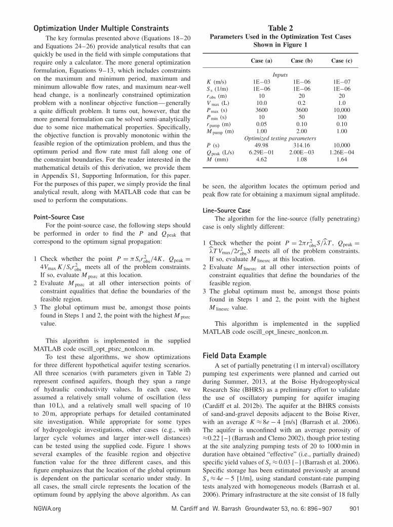
To test these algorithms, we show optimizationsfor three different hypothetical aquifer testing scenarios.All three scenarios (with parameters given in Table 2)represent confined aquifers, though they span a rangeof hydraulic conductivity values. In each case, weassumed a relatively small volume of oscillation (lessthan 10 L), and a relatively small well spacing of 10to 20 m, appropriate perhaps for detailed contaminatedsite investigation. While appropriate for some typesof hydrogeologic investigations, other cases (e.g., withlarger cycle volumes and larger inter-well distances)can be tested using the supplied code. Figure 1 showsseveral examples of the feasible region and objectivefunction value for the three different cases, and thisfigure emphasizes that the location of the global optimumis dependent on the particular scenario under study. Inall cases, the small circle represents the location of theoptimum found by applying the above algorithm. As can

Table 2Parameters Used in the Optimization Test Cases

Shown in Figure 1

Case (a) Case (b) Case (c)

InputsK (m/s) 1E−03 1E−06 1E−07S s (1/m) 1E−06 1E−06 1E−06robs (m) 10 20 20V max (L) 10.0 0.2 1.0Pmax (s) 3600 3600 10,000Pmin (s) 10 50 100rpump (m) 0.05 0.10 0.10M pump (m) 1.00 2.00 1.00

Optimized testing parametersP (s) 49.98 314.16 10,000Qpeak (L/s) 6.29E−01 2.00E−03 1.26E−04M (mm) 4.62 1.08 1.64

be seen, the algorithm locates the optimum period andpeak flow rate for obtaining a maximum signal amplitude.

Line-Source CaseThe algorithm for the line-source (fully penetrating)

case is only slightly different:

1 Check whether the point P = 2πr2obsS/̂λT , Qpeak =

λ̂T Vmax/2r2obsS meets all of the problem constraints.

If so, evaluate M linesrc at this location.2 Evaluate M linesrc at all other intersection points of

constraint equalities that define the boundaries of thefeasible region.

3 The global optimum must be, amongst those pointsfound in Steps 1 and 2, the point with the highestM linesrc value.

This algorithm is implemented in the suppliedMATLAB code oscill_opt_linesrc_nonlcon.m.

Field Data ExampleA set of partially penetrating (1 m interval) oscillatory

pumping test experiments were planned and carried outduring Summer, 2013, at the Boise HydrogeophysicalResearch Site (BHRS) as a preliminary effort to validatethe use of oscillatory pumping for aquifer imaging(Cardiff et al. 2012b). The aquifer at the BHRS consistsof sand-and-gravel deposits adjacent to the Boise River,with an average K ≈ 8e − 4 [m/s] (Barrash et al. 2006).The aquifer is unconfined with an average porosity of≈0.22 [–] (Barrash and Clemo 2002), though prior testingat the site analyzing pumping tests of 20 to 1000 min induration have obtained “effective” (i.e., partially drained)specific yield values of Sy ≈ 0.03 [–] (Barrash et al. 2006).Specific storage has been estimated previously at aroundS s ≈ 4e − 5 [1/m], using standard constant-rate pumpingtests analyzed with homogeneous models (Barrash et al.2006). Primary infrastructure at the site consist of 18 fully

NGWA.org M. Cardiff and W. Barrash Groundwater 53, no. 6: 896–907 901

Figure 1. Three examples of constrained optimization of oscillatory pumping. Colored area shows objective function value(signal magnitude), with lines representing implemented constraints. The circle in each case represents the optimal parameterset chosen, based on the supplied MATLAB code. Visual inspection of the full objective function plot shows that the optimumfound is the location of the largest feasible signal magnitude. Note that in each case a different set of optimization constraintsis active (i.e., the optimum does not always fall along the same constraint boundary).

penetrating wells screened throughout the sand-and-gravelformation and completed into an underlying aquitard.The central well field consists of a central well (A1)surrounded by two roughly concentric “rings” of six wellseach (B1 to B6 wells and C1 to C6 wells). Lastly a set offive wells (X1 to X5) surround the central well field andprovide the ability to monitor boundary condition impacts.Other wells, piezometers, and monitoring instrumentationhave been installed at the site throughout its history, andnumerous characterization efforts have been performedincluding hydrologic and geophysical methods. A fullsummary of site activities is beyond the scope of thetext, though the interested reader is directed to our priorpublications that describe site design and testing results(Barrash et al. 1999, 2006; Barrash and Clemo 2002;Cardiff et al. 2009, 2011, 2012a, 2013b), as well as tothe site webpage at http://cgiss.boisestate.edu/bhrs/.

An oscillating in-well “piston” design was developedin which a metal shaft with maximum stroke length0.91 m (for a total displacement of ≈1.85 L) would beused to cause injection and extraction of water from thedesired testing interval without removing water from thewell or pumping water into the well from the surface. Apiston at the land surface was moved by an electric motorconnected to a crankshaft which converted rotationalenergy to reciprocal motion. The surface piston was thenhydraulically connected to a sealed, down-hole pistonbelow the water table which acted on a 1-m aquifer inter-val, sealed above and below with packers. This down-holepiston thus directly forced water into the formation at thegiven testing interval during downward piston movementand pulled water out of the formation during upwardpiston movement. Based on the engine used and gearing,it was estimated that the OSG would be able to produceoscillation periods between roughly 1 and 100 s.

Before performing field experiments, we utilizedthe developed equations to determine the feasibility ofoscillatory pumping tests based on the above design

constraints. Because the pumping tests planned wouldperform oscillations within a small interval in the aquifer,we chose to use the point-source set of formulas asan approximation to predict responses. The Black andKipp (1981) formulas, as noted earlier, assume an aquiferunder confined conditions with infinite extent in allthree directions. This is a very rough approximationof the BHRS aquifer, which has a saturated thicknessof about 16.5 m during the Summer testing period.In order to apply the developed formulas, a singlerepresentative value for aquifer storage must also bechosen. This again requires a rough approximation ofthe BHRS aquifer that experiences both compressivestorage and water table (drainable) storage. Based onprior experience, the representative storage value waschosen to be equal to the specific storage coefficient of4e − 5 [1/m]. This approximation was deemed reasonablebased on observations of the amount of time required(10 min or more) to achieve representative “late time”storage behavior during constant-rate pumping tests(Barrash et al. 2006), though it should be noted thatthis approximation can be expected to be less accuratewhen pumping takes place near the water table. Ameasurement radius of 15 m between oscillating pumpingand observation locations was chosen, representing someof the larger distances expected from the test design.

Using the parameters above, the simpler formulationconsidering only volume constraints (Equations 18–20)yields: P̂ ≈ 9 s, Q̂peak ≈ 0.65 L/s, and M̂ ≈ 0.6 mm.Notably, this period of oscillation was well within therange expected to be possible with the planned OSG,and a head-change magnitude of 0.6 mm (or 1.2-mmpeak-to-trough amplitude) was known to be measur-able with the fiber-optic pressure sensors planned foruse. The additional constraint of ensuring reasonabledrawdowns/pressure build-ups near the pumping well isimportant at the BHRS aquifer, so we additionally appliedthe constrained optimization in which the casing radius

902 M. Cardiff and W. Barrash Groundwater 53, no. 6: 896–907 NGWA.org

Figure 2. Results of optimization of field testing plan for theBHRS. Circle shows optimal value obtained by applicationof formulas. Colored area shows feasible region for thisapplication, showing a range of periods across which signalsof 1 mm or greater are expected to be detectable.

of the pumping well, rwell, was set to 0.05 m, and themaximum head changed allowed at the casing radius wasM pump = 1 m. Cycle periods of 1 − 100 s were used asconstraints for the period. The results of the constrainedoptimization are shown in Figure 2, where an optimumperiod of P̂ ≈ 11.5 s is obtained. The optimum being atthis slightly longer pumping period is due to the near-wellhead-change constraint (i.e., formula 13), but does notresult in a significant change in the optimum signal magni-tude (M̂ = 0.58 mm). The gentle decrease in the objectivefunction in Figure 2 also shows that there is a fairlybroad range of periods across which oscillating testing isexpected to yield measurable signals at a distance of 15 m.

Field testing was carried out during July 2013 usingthe piston OSG described earlier. Examples of rawobservation data obtained from the BHRS testing areshown on the left in Figure 3, for four different oscillationperiods. In each of these tests, oscillations were inducedin a 1-m interval in a testing well (B3), with the intervalcentered at roughly 5 m below the water table. Theresponses shown represent pressure changes in a welllocated 10.55 m away laterally (C4), in a 1-m observationinterval centered 10.6 m below the water table. Giventhe site geometry, the data here represent head-changesignals collected by a transducer located 11.83 m totaldistance from the oscillating pumping location. Coherentsignals in the raw data demonstrate that even small-volume oscillations (≈0.45 L was used in this case)are measurable over distances of ≈12 m. The frequencyspectra for these signals (Figure 3, right) show thatpower on the order of 0.4 to 0.7 mm head change isobserved for tests at periods of 8 to 25 s with the highestpeaks occurring when the pumping period is around 14 s(Figure 3c). It should be noted that secondary peaks

can be found in many of these frequency spectra, andrepresent harmonics of the fundamental testing frequency.This is due to the fact that the oscillatory testing apparatusproduced a periodic but not exactly sinusoidal stimulation.Similarly to the results predicted by the pre-test analyses(Figure 2), high signal powers are produced even atlonger stimulation periods than the predicted 9- to 12-s optimum, though they decrease somewhat at longerperiods (Figure 3a and 3b) and appear to rapidly attenuateat shorter periods (Figure 3d).

Sensitivity AnalysisSteady-periodic theory can be used to derive sensi-

tivity maps that show the sensitivity of measurements toparameters such as spatially distributed K and S s. Theseanalyses show that measurements, such as signal ampli-tude and phase recorded at an observation well, havedifferent averaging volumes associated with different test-ing periods. Perhaps unsurprisingly, tests at short peri-ods (high frequencies) are more dependent on near-fieldaquifer heterogeneities, whereas longer period (lower fre-quency) tests are sensitive to aquifer heterogeneities overa larger volume.

One method for investigating the “averaging volume”associated with aquifer testing is through adjoint sen-sitivity analyses (see, e.g., formulations in Sykes et al.1985; Neupauer and Wilson 1999; Cirpka and Kitanidis2001; Cardiff and Kitanidis 2008), which provide math-ematical expressions for computing the sensitivity of anobservation to spatially distributed aquifer properties. Themost common use of adjoint sensitivity calculations is inthe numerical computation of spatial sensitivities requiredduring tomographic inverse problems. However, adjointsensitivity integrals can also be combined with analyti-cal (homogeneous) solutions. Sensitivity maps derived inthis way represent the linearized sensitivity of an obser-vation to perturbations in aquifer parameters throughoutthe domain. As an example, Leven and Dietrich (2006)present an analysis showing how the Theis solution canbe combined with adjoint state theory to understand thesensitivity of constant-rate pumping test observations tospatially distributed aquifer heterogeneity. In this section,we present a similar analysis for the case of oscillatingflow tests at different frequencies. We first review thekey formulas used to compute adjoint state sensitivitiesfor oscillatory flow problems and then show how ana-lytical solutions can be used to develop sensitivity mapsquickly. These maps provide a visual explanation of thechanges in the sensed region of an aquifer under dif-ferent pumping frequencies, and can be used to assesswhat portion of an aquifer is being interrogated by agiven testing design (i.e., the well locations and oscillatoryperiod).

Adjoint TheoryAs developed in Cardiff et al. (2013a), for an infinite

domain �, the sensitivity of a measurement mi to a

NGWA.org M. Cardiff and W. Barrash Groundwater 53, no. 6: 896–907 903

Time (s) Period (s)

Po

wer

(m h

ead

ch

an

ge)

Pre

ssu

re c

han

ge (

m h

ead

)

100 110 120 130 140 150 160 170 180 190 200−2

−1.5

−1

−0.5

0

0.5

1

1.5

2 x 10−3

0 5 10 15 20 25 300

0.2

0.4

0.6

0.8

1 x 10−3

100 110 120 130 140 150 160 170 180 190 200−2

−1.5

−1

−0.5

0

0.5

1

1.5

2 x 10−3

0 5 10 15 20 25 300

0.2

0.4

0.6

0.8

1 x 10−3

100 110 120 130 140 150 160 170 180 190 200−2

−1.5

−1

−0.5

0

0.5

1

1.5

2 x 10−3

0 5 10 15 20 25 300

0.2

0.4

0.6

0.8

1 x 10−3

100 110 120 130 140 150 160 170 180 190 200−2

−1.5

−1

−0.5

0

0.5

1

1.5

2 x 10−3

0 5 10 15 20 25 300

0.2

0.4

0.6

0.8

1 x 10−3

(a)

(g)

(b)

(d)

(c)

(e)

(f)

(h)

Figure 3. Field data from the BHRS 2013 testing campaign. 100 s of raw data at four different periods (left), and frequencyspectra (right) showing strong peaks at the testing frequency and associated harmonics.

parameter value p is found using the adjoint stateformulation as:

∂mi

∂p=

∫�

iωψi

∂Ss

∂p�ω + ∂K

∂p∇�ω· ∇ψi d�, (27)

where ω is the angular frequency of the testing, �ω is thephasor solution at that frequency, and K and S s representassumed average conductivity and storage parametersfor an aquifer. The variable ψ i is the so-called “adjointfield variable,” which is used in sensitivity calculation.For the case of a point observation, the adjoint fieldsolution is found by solving the steady-periodic flowproblem with an appropriate point-source term located atthe observation point.

In particular, an intuitive set of signal metricsdescribing response at an observation point are theamplitude and phase offset of the measured signal (withphase measured relative to the source signal). As shownin the appendix of Cardiff et al. (2013a), this can berepresented by defining a complex-valued observation

mi that contains the log-amplitude and phase (i.e., thecomplex modulus and complex argument) as its real andimaginary components:

mi =∫

�

ri d� (28)

ri = [ln (|�ω|) + i arg (�ω)

]δ (x − xi ) (29)

where xi is the location of measurement i . The mathe-matical details and background for this choice are beyondthe scope of this work, but can be found in the referencegiven above. The key result, however, is that the adjointsource term for such an observation should be equal to:

∂ri

∂�ω

= 1

�ω

δ (x − xi ) (30)

that is, a point source with magnitude 1/�ω.We now combine the adjoint state equations above

with the analytical solutions developed by Black and

904 M. Cardiff and W. Barrash Groundwater 53, no. 6: 896–907 NGWA.org

Kipp (1981) for point-source and line-source solutions.This makes it possible to generate sensitivity mapsthat can be used to understand the averaging volumesassociated with testing at different periods. The key stepsto performing such an analysis are outlined below, andan implementation of this process can be found in thesupplied MATLAB codes oscill_sens_linesrc_vis.m andoscill_sens_ptsrc_vis.m, along with their associated calledfunctions.

1 Supply the location of the oscillating pumping well,the maximum flow rate Qpeak, the angular frequency ofoscillation ω, the location of the observation well, andapproximate estimates of the aquifer conductivity andstorage parameters.

2 The phasor-domain solution, �ω, is given by theappropriate 2D or 3D (Black and Kipp 1981)solution.

3 Calculate the phasor value of the Black and Kipp (1981)solution at the location of the observation well, and callthis �obs.

4 The adjoint solution, ψ i, is given by the appropriate 2Dor 3D Black and Kipp (1981) solution with Qpeak setequal to 1/�obs.

5 Based on Equation 27, the sensitivity map of signallog-magnitude or phase to conductivity or storageparameters can be found through the appropriate innerproduct:

• Sensitivity of log-amplitude, ln(|�ω|), to ln(K ):Re(K∇�ω · ∇ψ i ).

Figure 4. Example of sensitivity maps produced through combination of analytical solution with adjoint theory. Sensitivitiesare unitless sensitivity of ln(signal amplitude) to ln(K ) and ln(S s). All maps use the same scale, with red representing positiveand blue representing negative sensitivities. Note broadening and diffusion of the sensitivity structure at larger periods.

NGWA.org M. Cardiff and W. Barrash Groundwater 53, no. 6: 896–907 905

• Sensitivity of log-amplitude, ln(|�ω|), to ln(S s):Re(iωψ i S s�ω).

• Sensitivity of phase, arg(�ω), to ln(K ):Im(K∇�ω · ∇ψ i )

• Sensitivity of phase, arg(�ω), to ln(S s):Im(iωψ i S s�ω).

Example VisualizationsWe now present one example of how these computa-

tions can be used to assess spatial sensitivity of measure-ments to aquifer parameters. This example considers anaquifer with diffusivity (K /S s) equal to 1, and with a pairof pumping/observation wells spaced 5 m apart, located at(−2.5, 0) and (2.5, 0), respectively.

In Figure 4, the spatial sensitivity structure ofln(amplitude) to aquifer parameters is shown across arange of testing periods. While the shortest testing periodof 0.1 s may be physically unreasonable, it emphasizesthe message that at very short testing periods, thesensitivity is almost entirely contained between thepumping and observation wells. As longer periods areused, the sensitivity structure broadens and “diffuses”outward, showing that these tests will be sensitive toaquifer parameters over a broader area.

These maps emphasize that oscillatory testing dataat different stimulation periods should be interpretedcarefully, since data from different periods of testing(if fit using a homogeneous model) may produce dif-ferent “effective” aquifer parameters. This is simplya manifestation of the different averaging volumesof these tests, and may help to explain the “intrinsicperiod-dependence” of hydraulic properties observed byboth Renner and Messar (2006) and Becker and Guiltinan(2010) in previous analyses.

Summary and ConclusionsOscillatory pumping tests are not presently a widely

used strategy for aquifer characterization. However, thebenefits associated with these tests (such as no net waterextraction, and multi-frequency sensitivity to differentaveraging volumes or scales) may prove useful forcontaminated site investigation and other purposes. In thispaper, we have developed several analytical tools thatcan be used to design and analyze oscillatory pumpingtests. While the background mathematics for someof these tools is fairly involved—using phase-domainmathematics—all key results can be applied immediatelywith pencil and paper, or through MATLAB programsusing a laptop computer. It is the authors’ hope thatthese simple tools will make the application of oscillatorypumping tests more approachable, and will produceeffective designs for oscillatory testing in the field.

We first presented a set of formulas that can beused to choose appropriate oscillatory pumping testdesign parameters, given only limited knowledge ofbulk or “effective” aquifer properties. Based on theaquifer parameters and a planned machinery design, the

key formulas presented (Equations 18–20 and Equations24–26) can be used to quickly determine reasonabletesting strategies. With significant design constraints,simple MATLAB codes can be used to verify testingfeasibility. After using this approach to develop a testingstrategy for a field campaign at the BHRS in Boise, ID,we showed how results from the field testing indicate thatthe testing design parameters used were well-optimized.

Secondly, we presented a method for understandinghow the response to an oscillatory pumping test will bedependent on spatially distributed aquifer parameters. Thecode presented uses analytical solutions for oscillatorytests coupled with an adjoint sensitivity analysis to quicklyand analytically derive sensitivity maps. Again, by usingonly a simple MATLAB program and bulk estimates ofaquifer parameters, a field practitioner can understand thespatial volume or scale “covered” by a given oscillatorypumping test, and how this sensitivity changes as afunction of the oscillatory testing period.

AcknowledgmentsThis work was supported by NSF Awards

1215746 and 1215768, and by ARO URISP awardW911NF1110291. Additional computational resourceswere provided by the UW-Madison Center for High-Throughput Computing (CHTC) and the AdvancedComputing Initiative (ACI). Cost share and design inputby Mt. Sopris Instruments (especially, James Koerlin)for development of the oscillating signal generator isgratefully acknowledged. The authors thank colleaguesDavid Hochstetler, Tania Bakhos, Peter K. Kitanidis,YaoQuan Zhou, and Michael Thoma, all of whomtook part in design and field data collection for theoscillatory pumping test data presented in this work.Finally, the authors thank reviewers Keith J. Halford andHund-Der Yeh, whose comments greatly contributed tothe refinement of this manuscript.

Supporting InformationAdditional Supporting Information may be found in theonline version of this article:

Appendix S1. Appendix containing a full derivation ofthe algorithm for determining period/flow rate optima forthe case where multiple testing constraints are considered.Appendix S2. A .zip file containing MATLAB codesdescribed in this paper, along with “click to run”supporting codes. Please view the README.TXT withinthe .zip file for further information.

ReferencesBakhos, T., M. Cardiff, W. Barrash, and P.K. Kitanidis.

2014. Data processing for oscillatory pump-ing tests. Journal of Hydrology 511: 310–319.DOI:10.1016/j.jhydrol.2014.01.007.

Barrash, W., and T. Clemo. 2002. Hierarchical geostatisticsand multifacies systems: Boise Hydrogeophysical Research

906 M. Cardiff and W. Barrash Groundwater 53, no. 6: 896–907 NGWA.org

Site, Boise, Idaho. Water Resources Research 38, no. 10:1196.

Barrash, W., T. Clemo, J.J. Fox, and T. Johnson. 2006.Field, laboratory, and modeling investigation of the skineffect at wells with slotted casing, Boise Hydrogeophys-ical Research Site. Journal of Hydrology 326: 181–198.DOI:10.1016/j.jhydrol.2005.10.029.

Barrash, W., T. Clemo, and M.D. Knoll. 1999. Boise Hydrogeo-physical Research Site (BHRS): Objectives, design, initialgeostatistical results. In Symposium on the Application ofGeophysics to Engineering and Environmental Problems(SAGEEP). Oakland, California: Environmental and Engi-neering Geophysical Society.

Becker, M., and E. Guiltinan. 2010. Cross-hole periodichydraulic testing of inter-well connectivity. StanfordGeothermal Workshop. Stanford, California: Stanford Uni-versity.

Black, J.H., and K.L. Kipp Jr. 1981. Determination of hydro-geological parameters using sinusoidal pressure tests: Atheoretical appraisal. Water Resources Research 17, no. 3:686–692. DOI:10.1029/WR017i003p00686.

Butler, J.J. Jr. 1998. The Design, Performance, and Analysis ofSlug Tests . Boca Raton, Florida: Lewis Publishers.

Cardiff, M., and P.K. Kitanidis. 2008. Efficient solutionof nonlinear, underdetermined inverse problems with ageneralized PDE model. Computers and Geosciences 34:1480–1491. DOI:10.1016/j.cageo.2008.01.013.

Cardiff, M., T. Bakhos, P.K. Kitanidis, and W. Barrash.2013a. Aquifer heterogeneity characterization with oscil-latory pumping: Sensitivity analysis and imaging poten-tial. Water Resources Research 49, no. 9: 5395–5410.DOI:10.1002/wrcr.20356.

Cardiff, M., W. Barrash, and P.K. Kitanidis. 2013b. Hydraulicconductivity imaging from 3-D transient hydraulictomography at several pumping/observation densities.Water Resources Research 49, no. 11: 7311–7326.DOI:10.1002/wrcr.20519.

Cardiff, M., W. Barrash, and P.K. Kitanidis. 2012a. A fieldproof-of-concept of aquifer imaging using 3D tran-sient hydraulic tomography with temporarily-emplacedequipment. Water Resources Research 48: W05531.DOI:10.1029/2011WR011704.

Cardiff, M., W. Barrash, and P.K. Kitanidis. 2012b. Oscilla-tory hydraulic tomography: Numerical studies. In Compu-tational Methods in Water Resources (CMWR). Champaign,Illinois: University of Illinois at Urbana-Champaign.

Cardiff, M., W. Barrash, B. Malama, and M. Thoma. 2011.Information content of slug tests for estimating hydraulicproperties in realistic, high-conductivity aquifer sce-narios. Journal of Hydrology 403, no. 1–2: 66–82.DOI:10.1016/j.jhydrol.2011.03.044.

Cardiff, M., W. Barrash, P.K. Kitanidis, B. Malama, A.Revil, S. Straface, and E. Rizzo. 2009. A potential-basedinversion of unconfined steady-state hydraulic tomography.Ground Water 47, no. 2: 259–270. DOI:10.1111/j.1745-6584.2008.00541.x.

Cirpka, O.A., and P.K. Kitanidis. 2001. Sensitivities of temporalmoments calculated by the adjoint-state method and jointinversing of head and tracer data. Advances in WaterResources 24, no. 1: 89–103.

Fokker, P.A., J. Renner, and F. Verga. 2013. Numericalmodeling of periodic pumping tests in wells penetrating aheterogeneous aquifer. American Journal of EnvironmentalSciences 9: 1–13.

Hollaender, F., P.S. Hammond, and A. Gringarten. 2002. Har-monic testing for continuous well and reservoir monitoring.

Paper SPE 77692 presented at the 2002 SPE Annual Tech-nical Conference and Exhibition, San Antonio, Texas.

Jazayeri Noushabadi, M.R., H. Jourde, and G. Massonnat.2011. Influence of the observation scale on permeabilityestimation at local and regional scales through well testsin a fractured and karstic aquifer (Lez aquifer, SouthernFrance). Journal of Hydrology 403, no. 3–4: 321–336.DOI:10.1016/j.jhydrol.2011.04.013.

Johnson, C.R., R. Greenkorn, and E. Woods. 1966. Pulse-testing:A new method for describing reservoir flow propertiesbetween wells. Journal of Petroleum Technology 18, no.12: 1599–1604.

Kuo, C.H. 1972. Determination of reservoir properties fromsinusoidal and multirate flow test in one or more wells.SPE Journal 12, no. 6: 499–507.

Lavenue, M., and G. de Marsily. 2001. Three-dimensionalinterference test interpretation in a fractured aquifer usingthe Pilot Point Inverse Method. Water Resources Research37, no. 11: 2659–2675. DOI:10.1029/2000wr000289.

Leven, C., and P. Dietrich. 2006. What information canwe get from pumping tests?—Comparing pumping testconfigurations using sensitivity coefficients. Journal ofHydrology 319: 199–215.

Maineult, A., E. Strobach, and J. Renner. 2008. Self-potential signals induced by periodic pumping tests.Journal of Geophysical Research 113, no. B01203: 12.DOI:10.1029/2007JB005193.

McElwee, C.D., B.R. Engard, B.J. Wachter, S.A. Lyle, J. Healey,and J.F. Devlin. 2011. Hydraulic tomography and high-resolution slug testing to determine hydraulic conductivitydistributions. KGS Open-File Reports (2011-02): 168.

Neupauer, R.M., and J.L. Wilson. 1999. Adjoint methodfor obtaining backward-in-time location and travel timeprobabilities of a conservative groundwater contaminant.Water Resources Research 35, no. 11: 3389–3398.

Rasmussen, T.C., K.G. Haborak, and M.H. Young. 2003.Estimating aquifer hydraulic properties using sinusoidalpumping at the Savannah River site, South Carolina, USA.Hydrogeology Journal 11: 466–482. DOI:10.1007/s10040-003-0255-7.

Renner, J., and M. Messar. 2006. Periodic pumping tests.Geophysical Journal International 167: 479–493.DOI:10.1111/j.1365-246X.2006.02984.x.

Revil, A., C. Gevaudan, N. Lu, and A. Maineult. 2008.Hysteresis of the self-potential response associated withharmonic pumping tests. Geophysical Research Letters 35,no. 16: L16402. DOI:10.1029/2008gl035025.

Rosa, A., and R. Horne. 1997. Reservoir description by well testanalysis using cyclic flow rate variation. SPE FormationEvaluation 12, no. 4: 247–254.

Smith, A.J. 2008. Weakly nonlinear approximation of periodicflow in phreatic aquifers. Ground Water 46, no. 2: 228–238.DOI:10.1111/j.1745-6584.2007.00418.x.

Sykes, J.F., J.L. Wilson, and R.W. Andrews. 1985. Sensitivityanalysis for steady state groundwater flow using adjointoperators. Water Resources Research 21, no. 3: 359–371.

Townley, L.R. 1993. AQUIFEM-P: A periodic finite elementaquifer flow model: User’s manual and description. CSIRODivision of Water Resources Technical Memorandum93/13. 72 pp, plus software.

Vela, S., and R. McKinley. 1970. How areal heterogeneitiesaffect pulse-test results. SPE Journal 10, no. 2: 479–493.

Yeh, H.-D., and Y.-C. Chang. 2013. Recent advances inmodeling of well hydraulics. Advances in Water Resources51: 27–51. DOI:10.1016/j.advwatres.2012.03.006.

NGWA.org M. Cardiff and W. Barrash Groundwater 53, no. 6: 896–907 907