Journal of Computational Physics 263 (2014) 91–112

Contents lists available at ScienceDirect

Journal of Computational Physics

www.elsevier.com/locate/jcp

Connecting the dots: Semi-analytical and random walknumerical solutions of the diffusion–reaction equation withstochastic initial conditions

Amir Paster a,c,∗, Diogo Bolster a, David A. Benson b

a Environmental Fluid Mechanics Laboratories, Dept. of Civil and Environmental Engineering and Earth Sciences, University of Notre Dame,Notre Dame, IN, USAb Hydrologic Science and Engineering, Colorado School of Mines, Golden, CO, 80401, USAc School of Mechanical Engineering, Tel Aviv University, Tel Aviv, 69978, Israel

a r t i c l e i n f o a b s t r a c t

Article history:Received 2 April 2013Received in revised form 17 November 2013Accepted 13 January 2014Available online 21 January 2014

Keywords:Diffusion–reaction equationBimolecular reactionIncomplete mixingParticle methodsRandom walk

We study a system with bimolecular irreversible kinetic reaction A + B → ∅ where theunderlying transport of reactants is governed by diffusion, and the local reaction term isgiven by the law of mass action. We consider the case where the initial concentrationsare given in terms of an average and a white noise perturbation. Our goal is to solvethe diffusion–reaction equation which governs the system, and we tackle it with bothanalytical and numerical approaches. To obtain an analytical solution, we develop theequations of moments and solve them approximately. To obtain a numerical solution, wedevelop a grid-less Monte Carlo particle tracking approach, where diffusion is modeled bya random walk of the particles, and reaction is modeled by annihilation of particles. Theprobability of annihilation is derived analytically from the particles’ co-location probability.We rigorously derive the relationship between the initial number of particles in the systemand the amplitude of white noise represented by that number. This enables us to comparethe particle simulations and the approximate analytical solution and offer an explanationof the late time discrepancies.

© 2014 Elsevier Inc. All rights reserved.

1. Introduction

The diffusion–reaction equation (DRE) is a common mathematical model used to describe the dynamics of systems wherethe interaction of reactants is facilitated by pure diffusion. These systems are ubiquitous and the DRE has been applied ina broad range of scientific fields, including chemistry [1], physics [2–5], biology [6], economics [7–9], social sciences [10],technology transfer [11], warfare studies [12] and ecology [13].

Consider the irreversible bimolecular kinetic reaction A + B → P . This elementary reaction can be regarded as the fun-damental building block of more complex reactions, which can be built as combinations of bimolecular and unimolecularcases [14]. For the sake of simplicity, the product P is neglected in the current study; hence, we focus on the reactionA + B → ∅. We assume the law of mass action is valid in a well-mixed system, i.e., the rate of reaction at a point is linearlyproportional to the product of concentrations of A and B at that point [15].

A classical experiment is to consider a reactive system with A and B uniformly mixed throughout with identical initialconcentration C A(x, t = 0) = C B(x, t = 0) = C0. For these deterministic initial conditions the evolution of concentrations canbe calculated exactly and is well known to scale like t−1 at late times. However, this relies explicitly on the assumption of

* Corresponding author at: School of Mechanical Engineering, Tel Aviv University, Tel Aviv, 69978, Israel.E-mail address: paster@tau.ac.il (A. Paster).

0021-9991/$ – see front matter © 2014 Elsevier Inc. All rights reserved.http://dx.doi.org/10.1016/j.jcp.2014.01.020

92 A. Paster et al. / Journal of Computational Physics 263 (2014) 91–112

a well-mixed deterministic initial condition. If the initial concentrations are stochastic instead of deterministic, i.e., they havesome random fluctuation about a mean concentration, the deterministic solution will eventually break down [2,5,16,17].

In particular, at late times the average concentrations drop, and if diffusion is not sufficiently strong to smooth outconcentration fluctuations, the fluctuations eventually can become comparable in size or indeed larger than the meanconcentration. Thus, areas in which one species is severely or completely depleted relative to the other develop in thedomain [2,4,5]. The phenomenon of formation of segregated areas, or islands, due to diffusion-limited kinetics, is known asOvchinnikov–Zeldovich segregation [18]. For reactions to actually occur, reactants have to be co-located, i.e. mixed. Hence,reaction inside islands is limited and mainly prevails on the edges, or interfaces, between them [18]. Thus, incomplete mix-ing results in a decrease in the overall rate of reaction, when compared with the anticipated rate of a well-stirred system[2,5,19,1,17,20]. The average concentration, which scales as t−1 in the well-mixed regime, will at late times scale as t−d/4,where d is the number of spatial dimensions [2,4,5,21].

This phenomenon of incomplete mixing was demonstrated experimentally by Monson and Kopelman [22,23] and similareffects are hypothesized as the reason why classical DRE predictions of reactive transport overestimate the reaction rate asmeasured in experiments. This has been observed in a variety of systems including, but not limited to, flow through porousmedia [24,25], turbulent flows [26], atmospheric flows [27,28] and biological systems [29].

The occurrence of incomplete mixing motivates improved predictions of mixing [30–36] so as to better predict mixingdriven reactive transport [37–44]. Thus, analytical and numerical models capable of capturing incomplete mixing effects aredesirable.

For the systems described above, which transition from well-mixed to segregated regimes, semi-analytical solutions forthe DRE have been developed by [21,17,45,46], assuming one-dimensional ergodic systems. These solutions were obtainedby decomposing the concentration into its ensemble mean and the deviation from it, and developing equations for themoments of concentration deviations. Then, an equation for the mean concentration is obtained by neglecting higher ordermoments and assuming idealized initial conditions. Finally, an analytical solution of this equation is obtained.

A variety of stochastic simulation algorithms have been introduced to simulate chemical reactions, many of which arebuilt (e.g., [47]) to replicate the models of Smoluchowski [48] or Doi [49]. Both models assume reactions occur when par-ticles are within some interaction radius, the physical basis of which is still subject to debate due to the discrete andlinked (i.e., many-body) nature of the reactions, combined with larger-scale correlations in particle number densities [50]that may exist. Other models take a more macroscopic approach, including Gillespie’s stochastic simulation algorithm (SSA)[14], which assumes perfect mixing in a volume of d-dimensional space (voxel). Such grid-based approaches, such as Cel-lular Automata [51], particle-grid methods [52] and modified lattice-based Gillespie algorithms [20] typically involve theassumption that a grid cell is well-mixed. This assumption is justified if the characteristic diffusion time across the cell ismuch smaller than the characteristic reaction time [53]. Further extensions that allow for spatial inhomogeneity by furthersubdividing space into many voxels of size hd are hampered by the fact that reactions disappear as h → 0, because theprobability of A and B particles coexisting in the same voxel goes to zero. To address this, Isaacson [54] allows reactions totake place among a rigorously-defined neighborhood of voxels, across which perfect mixing prevails. Isaacson [54] favorablycompares his results to a Brownian Dynamics simulation [47], in which particles move according to a Gaussian Brownianmotion and react according to a rate dictated by continuum diffusion to a fixed (absorbing) reaction radius in the mannerof Smoluchowski’s model. In doing so, Isaacson shows that the spatial Gillespie method can be modified to converge to acontinuous-space particle method. However, in most current voxel-based methods, diffusion is approximated with randommass transfer between nearest-neighbor cells, effectively enforcing finite support and ruling out non-local forms of masstransfer. Additionally, grid-free Lagrangian methods such as Smooth Particle Hydrodynamics (SPH) have also emerged [37,38]. In SPH, Lagrangian fluid parcels carry masses of reactants, and reactions within each parcel are calculated assumingthat it is well-mixed. Thus, similar limitations apply.

A common Lagrangian model for conservative solute transport is the random walk particle tracking method (PT) [55–57].While it is straightforward to incorporate first order reactions A → ∅ in PT [58–60], a salient question is how to incorporatethe bi-molecular case A + B → P . One approach is to define an effective reaction radius as noted above, and if the distancebetween a reactive particle pair is smaller than this radius, they can react [61,62,39]. However, other than at the molecularscale, this effective radius can be regarded as a tuning parameter whose physical meaning is unclear. Alternatively, a mixedEulerian–Lagrangian approach maps discrete particle locations onto a grid of concentrations, where reaction rates are cal-culated and then masses re-interpolated back onto Lagrangian particles [52]. However, this approach is computationallyinefficient and still assumes the grid cell is well-mixed. A novel reactive PT (RPT) method was proposed by Benson andMeerschaert [63], where particles carry uniform masses of reactants A or B , and in every time step move by a classicalrandom walk. At any time, each particle pair of reactants will have a (unique) probability to react with each other. Thisprobability follows rigorously and directly from the principles of the law of mass action and Brownian motion [64]. Theprobability is proportional to the reaction rate as well as the co-location probability density associated with the distancebetween particle pairs. Hence, particles that are close together have a higher probability of reaction than particles who arefar apart. In [64] the authors showed that the algorithm of [63] converges to the diffusion–reaction equation.

The RPT algorithm of Benson and Meerschaert [63] is similar in concept to the Green’s function approach of [65], withsome exceptions. First, van Zon and ten Wolde [65] choose a maximum timestep that is tied to limiting every particle tointeracting with only its nearest neighbor. The algorithm of [63] calculates collision probabilities with all nearby partners andthe reactions proceed on a stochastic basis. Second, the algorithm in [63] does not define a fixed radius of interaction and is

A. Paster et al. / Journal of Computational Physics 263 (2014) 91–112 93

not restricted to diffusive motion of particles; it can be extended to spatially non-local processes such as Lévy motion [17],where a simple interaction radius may be impossible to define. Third, Benson and Meerschaert [63] maintain a non-zerosurvival probability when particles are collocated. The probability of reaction is the product of independent probabilitiesof collision and reaction given a collision. For fast reactions the probability of reaction given a collision is high, while forslow reaction it may be low. Their original study [63] only considered a one-dimensional case, but showed that this RPTscheme naturally transitions from the well-mixed t−1 regime to the incompletely mixed t−1/4 one. We have extended theRPT approach to d = 2,3 and have shown that it converges to the appropriate DRE equation in the limit of small time step[64]. This RPT method has been shown to reproduce experimentally observed reaction rates, where classical well-mixedmodels fail to match observed reaction rates [66].

In this paper we explore the connection between the RPT numerical method and semi-analytical solutions of the DRE.In Section 2, we derive an approximate d-dimensional semi-analytical solution of the mean concentration, for the casewhere C A(t = 0) = C B(t = 0) = C0. The solution approach is based on the moment equation method and is for any generald-dimensional system, extending the 1-d approaches of [21,17,45]. In Section 3 we describe in detail the numerical RPTapproach in d dimensions; we formally quantify the stochastic nature of the initial condition, discuss numerical approxima-tions of the algorithm and derive time stepping limitations for the algorithm. In Section 4 we compare the results of the RPTmodel and the semi-analytical model, and offer explanations for any discrepancies between the two models, particularly atlate times.

2. Analytical model

2.1. System definition and governing equations

We consider a bimolecular reactive system where transport of constituents is driven by diffusion. Two components inthis system, A and B , react kinetically and irreversibly with one another such that A + B → ∅. For simplicity, we assumethat the product of the reaction plays no role in the system and can be neglected. For an infinite d-dimensional space thegoverning equation for transport of the components is the diffusion–reaction equation (DRE)

∂Ci

∂t= D∇2Ci − kC A C B , i = A, B − ∞ < x < ∞, (1)

where the concentration of component i is given by Ci = Ci(x, t) [mol L−d], D is the diffusion coefficient [L2 T−1], andk [Ld mol−1 T−1] is the reaction rate constant. The reaction rate r = kC A C B is assumed to be given by the law of massaction.

2.2. Solution for well-mixed system

When the system is well-mixed in space at all times, concentrations are constant in space and the diffusion term inEq. (1) can be dropped. For this case, called the thermodynamic limit, well-known analytical solutions exist. For the simplestcase, where the initial average concentrations are equal C A(t = 0) = C B(t = 0) = C0, Eq. (1) becomes ∂Ci/∂t = −kC2

i , and itssolution is

Ci(t) = C0

1 + C0kt, (2)

which scales as t−1 at late times.

2.3. Solution for a system with concentration fluctuations

Keeping the thermodynamic limit in mind, we are interested in the more complex case where concentrations have somerandom initial distribution, and the system is not continuously well mixed; for this setup concentration evolves by diffusionas described by the DRE (1). To this end, we decompose concentrations into mean and fluctuation terms, such that

Ci(x, t) = Ci(t) + C ′i(x, t), (3)

where the overbar refers to the ensemble average and the prime to the zero mean fluctuations about the average. Let usassume the system is ergodic, such that the ensemble average and spatial average are interchangeable, and only depend on t .Restrictions associated with the assumption of ergodicity are discussed, for example, in [45]. Broadly speaking the larger thephysical domain, the better the assumption of ergodicity as larger domains can carry the full ensemble of statistics. Let usalso assume that the initial concentration distributions of species A and B have identical statistical structure at t = 0. Theseassumptions allow us to obtain an analytical solution for the problem, but are not required for numerical simulation. Withthese assumptions, the spatial averages of the initial concentrations of A and B are equal, i.e.

C A(t = 0) = C B(t = 0) ≡ C0. (4)

94 A. Paster et al. / Journal of Computational Physics 263 (2014) 91–112

and clearly, due to the 1:1 stoichiometric ratio of the reaction, their average concentrations are equal for all t � 0, i.e.

C A(t) = C B(t) ≡ C(t). (5)

Substituting (3) into (1) and taking the ensemble average of the equation, we obtain an equation for the average con-centration such that

dC

dt= −k

(C2 + C ′

A C ′B

), (6)

where the last term C ′A C ′

B = C ′A(x, t)C ′

B(x, t) is the cross-covariance between concentration deviations. For a highly mixedsystem, this term is negligible compared to the other terms in the equation, but this is no longer the case when speciessegregation occurs. During segregation A and B typically develop anti-correlation so this term becomes negative, slowingthe mean reaction rate.

Ultimately, we want to solve for the average concentration C , but to do this we have to solve for the cross-covariance.With this in mind, we combine the equation for the mean concentration (6) into the DRE (1) to get

∂C ′i

∂t= D∇2C ′

i − kC(C ′

A + C ′B

) − kC ′A C ′

B + kC ′A C ′

B (7)

to obtain an evolution equation for the concentration deviation.

2.3.1. Moment equations and initial conditionsEquations for the evolution of the autocovariance f (x,y, t) = C ′

A(x, t)C ′A(y, t) and the cross-covariance g(x,y, t) =

C ′A(x, t)C ′

B(y, t) can be obtained from (7). Details of the derivation are given in Appendix A; the resulting moment equationsare

∂ f

∂t= 2D∇2 f − 2k

[C(t)( f + g) + h1

], (8)

∂ g

∂t= 2D∇2 g − 2k

[C(t)( f + g) + h1

], (9)

where

h1(x,y, t) = C ′A(x, t)C ′

B(x, t)C ′A(y, t) (10)

is a third order moment. Taking the sum and the difference of (8) and (9), we get two independent equations for f + g andf − g ,

∂

∂t( f + g) = 2D∇2( f + g) − 4k

[C(t)( f + g) + h1

],

∂

∂t( f − g) = 2D∇2( f − g). (11)

An approximate solution of these equations, subject to specified initial conditions, can be obtained by neglecting thethird order moment h1. This is justified when |C A(t)( f + g)| |h1|. We shall later return to examine this assumption, usingresults from numerical simulations.

Various initial conditions could be assumed for f and g . Since we are ultimately interested in showing the correlationbetween numerical particle models and the analytical solutions of the system, we will focus on synthetic initial conditionsthat match those imposed in the numerical simulations (see next section). Thus we assume that the cross-covariance isidentically zero, whereas the autocovariance is described by a Dirac delta function, i.e.

f (x,y, t = 0) = σ 2ldδ(x − y),

g(x,y, t = 0) = 0, (12)

where σ 2 is the concentration variance and l the correlation length. For these initial conditions, the solutions of (11),neglecting h1, are

( f − g)(x,y, t) = σ 2ld

(8π Dt)d/2e− (x−y)2

8Dt ,

( f + g)(x,y, t) = σ 2ld

(8π Dt)d/2exp

[− (x − y)2

8Dt− 4k

t∫C(t′)dt′

]. (13)

0

A. Paster et al. / Journal of Computational Physics 263 (2014) 91–112 95

Taking the difference of Eqs. (13), and setting y = x,

g(x,x, t) = σ 2ld

2(8π Dt)d/2

(−1 + exp

[−4k

t∫0

C(t′)dt′

]), (14)

which can now be substituted into (6) to obtain a closed-form, albeit implicit, equation for the mean concentration:

dC

dt= −kC 2 − k

2

σ 2ld

(8π Dt)d/2

(−1 + e−4k∫ t

0 C(t′) dt′) (15)

subject to initial conditions C(t = 0) = C0. We were unable to obtain a closed form expression for the solution of Eq. (15),but it can be solved numerically. The details of the numerical solution are given in Appendix B.

3. Numerical particle tracking model

Benson and Meerschaert [63] proposed a numerical solution method for the diffusion–reaction equation by Monte Carlosimulations of reactive particle tracking (RPT). In their approach, transport and reaction of species is modeled by a largenumber of particles of constant mass, moving and interacting within a finite domain.

The purpose of using the RPT approach is to obtain a numerical solution for the problem at hand, as described by theDRE (1) and the initial conditions (4) and (12). The key advantage of the RPT approach over the analytical solution is thathigh order moments are not neglected within the RPT framework. However, RPT is computationally intensive and it canonly be applied to a finite domain for the problem at hand. The latter restriction affects the results at late times, as we shalldiscuss in detail in Section 4.

In the RPT approach, the diffusion of a species is modeled by a Brownian random walk, i.e., during a time step eachparticle moves by a random distance. The reaction term is modeled by evaluating both the probability of co-location ofparticles, which is derived from first principles using Brownian motion, and the probability of reaction given co-locationderived from the law of mass action (see [14]); it is not a closure or a sub-scale model.

Here we describe, extending the work of [63], how this approach is generalized to any number of dimensions d = 1,2,3.In all cases presented we consider a finite domain with periodic boundary conditions, but it is straightforward to implementothers. For the one-dimensional case, the domain is a line segment of length Ω; for higher dimensions, e.g. d = 2,3, thedomain is a hypercube (square or cube respectively), with edge length Ω , such that the volume of the domain is Ωd . Inthese simple domains, periodic boundary conditions are easy to implement.

3.1. Initialization of the simulation

First, we need to set the system of particles so that it complies with the initial condition (4), (12). To this end, N0 par-ticles of species A are spread randomly within the domain of size Ωd . The location of the i-th A particle is denoted byXAi , where 0 � X Ai < Ω . These initial particle locations are chosen by generation of independent and identically distributed(i.i.d.) random variables, i.e. the particles are uniformly distributed on the domain. The concentration field formed by theparticles in a single realization is given by

C A0(x) = C A(x,0) =N0∑

i=1

mpδ(x − XAi0), (16)

where the 0 subscript denotes the initial time, and mp [mol] is the number of moles carried by a single particle. Here, dueto the ergodicity of the system, mp has a constant value. The average concentration in the system is C0, so mp is given by

mp = C0Ωd/N0. (17)

The process of attributing random coordinates is repeated for the B particles. The locations of the A and B particles haveno correlation, so the initial cross-covariance of concentrations is zero,

C ′A(x,0)C ′

B(y,0) = 0. (18)

By contrast, as shown in detail in Appendix C, the autocovariance of the concentrations is approximately a delta function,

C ′A(x,0)C ′

A(y,0) = C ′B(x,0)C ′

B(y,0) = C20Ωd

N0δ(x − y), (19)

so the initial condition can be matched with (12) by imposing

C20Ωd

= σ 2ld. (20)

N0

96 A. Paster et al. / Journal of Computational Physics 263 (2014) 91–112

Thus, if the initial concentration statistics σ 2ld and C0 are known for a given system, the above expression determinesthe initial particle density, given by

ρ0 = C20

σ 2ld, (21)

where ρ0 = N0/Ωd . Surprisingly, this implies that in order to simulate a system of a given size with an initial condition

that contains a considerable noise, a small number of particles is needed; whereas, if the system has zero noise, an infinitenumber of particles is needed. The latter case is impractical, and thus our approach is deemed useful as long as there issome noise in the initial concentration of the system. Hence, noisier systems may be more suited to the RPT approach,since it requires less particles, and can be more computationally efficient. Note that noise in natural systems tends to beubiquitous [24–29]. With the particle density given by (21), we can now rewrite the number of moles carried by a singleparticle (17) as

mp = σ 2ld/C0. (22)

The above results can be generalized to the non-ergodic case, where the initial concentration statistics of the species aregiven as a function of x. Then, the expected density of the particles, and the number of moles carried by a single particleat location x, are given by

ρ0(x) = C0(x)2

ς(x), mp(x) = ς(x)/C0, (23)

where C0(x) and ς(x) = σ 2(x)ld(x) are the local mean concentration and white noise magnitude, respectively. While we donot use this generalization in this paper, we highlight it due to the very powerful flexibility in stochastic initial conditionsit provides.

3.2. Brownian motion

The right-hand side of the DRE (1) contains two terms: a diffusion and a reaction term. In a physical system, diffusionand reaction are simultaneous processes; reaction cannot take place without diffusion. In the numerical model these twocontributions are modeled by operator splitting, i.e., two subsequent processes within each simulation time step. First, theparticles move by Brownian motion, and then they can react with each other. We note that the order of these steps in thealgorithm can be interchanged without consequence.

The dispersive motion is modeled with a random walk, which in each dimension has zero mean and variance 2Dt ,where t is the length of the time step. For each particle and in each dimension 1 � k � d, we update the particle coordinateXk to be

(Xk + √2Dtξ) mod Ω, (24)

where ξ ∼ N (0,1) is a standard normal random variable with ξ = 0 and ξ2 = 1; and mod is the modulus operator. Thelatter imposes the periodic boundary conditions by bringing a particle which leaves the domain boundary back into thedomain through the other side. Note that an anisotropic diffusion can also be implemented with covariance matrix 2Dt.

3.3. Reaction decay

3.3.1. First order approximationThe second process is reaction, modeled during each time step as the probabilistic decay of a certain number of the

particles. Our algorithm loops over all A particles. For a given particle Ai , we search for “live” B particles that are locatedwithin a cutoff radius δ = O(

√8Dt ) of X Ai . This speeds calculations and is explained in detail in 3.3.3. We sequentially

loop through those B particles, Bk1 , Bk2 . . . ; for each one of them, denoted Bk j , we calculate the probability of reactionwith Ai . This reaction probability is given by the first order approximation

P f = P f (Ai, Bk j ) = kmp v(s,t)t, (25)

where v(s,t) denotes the co-location probability density function (PDF) and s = |XAi −XBk j| denotes the distance between

the particles. To grasp the meaning of the co-location PDF, consider the expression v(s,t)dV . This is the probability thatboth of the diffusing particles will be within some (arbitrarily located) infinitesimal volume dV .

In the isotropic case where D is constant, the location PDFs are Gaussians with variance 2Dt (see Fig. 1), and theco-location probability density is obtained by the convolving those two Gaussians [63]. The convolution yields a Gaussianwith double the variance, i.e. for a constant D the co-location PDF is

v(s,t) = 1d/2

e− s28Dt , (26)

(8π Dt)

A. Paster et al. / Journal of Computational Physics 263 (2014) 91–112 97

Fig. 1. Illustration of the convolution of two Gaussians in a one-dimensional case. Here, the particles are located at xA = 0 and xB = 1, such that s = 1,and 2Dt = 1. The green line depicts the product of the particles’ Gaussians. The hatched area underneath this line is the convolution of the Gaussians,v(s,t), as given by Eq. (26). (For interpretation of the references to color in this figure legend, the reader is referred to the web version of this article.)

Fig. 2. Flow chart for implementation of particle reaction in the algorithm. N A denotes the number of A particles at the current time step.

whose variance is 4Dt . Note that expression (26) can be extended to any types of motion; for example, anisotropicBrownian motion by replacing v(s) with a multi-Gaussian whose covariance matrix is 4Dt or by using approximations ofa stable density for Lévy motion [17].

Once the reaction probability P f for a given A, B couple is known, a random number U , uniformly distributed on [0,1],is generated. If P f � U , the reaction occurs and we “kill” both the Ai and Bk j particles, i.e., remove them from the system.We then continue to the next A particle, Ai+1. On the other hand, if P f < U , we move on to the next close-by B particle,i.e. Bk j+1 , compute the reaction probability with that particle, compare to a new U , and so forth. The process is illustratedvisually in a flow chart in Fig. 2.

3.3.2. Justification of the first order approximationThe reaction probability can be, in general, calculated without using the first order approximation (25). To this end, one

can write the probability of survival of a particle during an infinitesimal time step as

P s(t′ + dt′) = P s

(t′)[1 −

∑kmp v

(si, t′)dt′

], (27)

i

98 A. Paster et al. / Journal of Computational Physics 263 (2014) 91–112

where t′ is the time, elapsed at the beginning of the time step, and the sum is over all neighboring particles. Thus, the rateof change of this probability is given by

dP s/P s = −∑

i

kmp v(si, t′)dt′ (28)

and by integration over a time step t , one can approximate the overall reaction probability during time step t as

P f = 1 − P s(t) = 1 − exp

[−kmp

∑i

t∫0

v(si, t)dt

]. (29)

We applied the expression (29) in RPT simulations and compared the results with ones from the approach based on thefirst order approximation (25), as described in Section 3.3.1. We have found that the results are practically identical, andtherefore adhere to the first order approximation, which is simpler to implement.

3.3.3. Cutoff distance and correction termDue to the periodic boundary conditions, the Ai particle can react with any of the B particles in the domain, and

with any of the imaginary B particles, reflected by the boundaries. There are an infinite number of such particle pairs,as the reflection is infinite. In practice, it is clear that distant particles have negligible probability of reaction and so forcomputational efficiency, a cutoff distance δ related to the co-location probability is placed in the neighbors search,

δ = a√

8Dt, (30)

where a is an arbitrary value, chosen large enough to not significantly affect the accuracy of the simulation. Through trialand error and convergence tests, we have found that a = 2 is high enough to give accurate results in the simulations.

Note that our approach for calculating the probability of reaction is slightly different from the work of Benson andMeerschaert [63]. They used a tent-shaped, piecewise linear function, truncated at δ = √

24Dt , whose integration yields 1(see Fig. 1b in [63]). In practice, if the time steps are small enough, their approach yields results which are similar to theresults obtained using our approach. Note that similar tent functions can be developed for d = 2,3.

In order to make the particle pair search numerically efficient it is performed using a k–d tree range search algorithm[67]. With the k–d tree approach, the numerical cost of the search is O(N A log NB), where N A , NB are the number ofparticles in the system. By comparison, a naïve search would be much more expensive at O(N A NB).

For theoretical consistency, the co-location probability density must integrate to unity [64]. Thus a correction factor mustbe included in (26) such that

v(s) ={

η−1 1(8π Dt)d/2 e− s2

8Dt s � δ,

0 s > δ,(31)

where η is found by integration of (26) to be

η =⎧⎨⎩

erf(a) d = 1,

1 − e−a2d = 2,

erf(a) − (2a/√

π )e−a2d = 3.

(32)

For example, if a = 2, then η ∼ 0.995,0.982,0.954 for d = 1,2,3, respectively. So, for this choice of cutoff distance, thecorrection in (31) is relatively small.

If all particles are consumed during the current time step, the simulation ends. Otherwise, the algorithm advances thetime counter tn+1 = tn + tn , and repeats the Brownian motion and reaction steps.

3.4. Restrictions on time discretization by the first order scheme

One of the features that has not been explored with this algorithm is how to select appropriate time-steps. For this studywe choose to use a first order scheme in time and here discuss in depth restrictions on the choice of time discretizationthat should be incorporated in the simulation as a result of the scheme. To start, let us switch to dimensionless variablesC∗ = C/C0 and t∗ = kC0t . Then expanding with a Taylor series we can write

C∗(t∗ + t∗) = C∗(t∗) + t∗ ∂C∗

∂t∗(t∗) + (t∗)2

2!∂2C∗

∂t∗2+ · · · , (33)

where the dots denote terms of higher order. We can justify neglecting second and higher order terms in our scheme if themagnitude of their sum is much smaller than the first order term, i.e.

|∑∞ν=2(ν!)−1C∗(ν)(x, t∗) (t∗)ν |

∗(1) ∗ ∗ � 1, (34)

|C (x, t )|t

A. Paster et al. / Journal of Computational Physics 263 (2014) 91–112 99

Fig. 3. Time discretization.

where C∗(ν) = ∂νC∗/∂(t∗)ν denotes the ν-th order derivative of C∗ , with respect to time. The expression on the LHS in(34) converges to zero as t → 0. Hence, the error of the numerical approach, when compared to the exact solution, getssmaller as t → 0. However, given that smaller time steps result in more computational cost, the question is, how big cant be, without violating requirement (34), and how big is the error induced by a specific choice of t?

At early times, we know that fluctuations in concentration play a negligible role and the well-mixed solution (2) is agood approximation of the actual concentration. The ν-th derivative of the well-mixed solution, C∗ = 1/(1 + t∗), is

C∗(ν) = ∂νC∗

∂(t∗)ν= ν!(−1)ν

(1 + t∗)ν+1. (35)

At late times, segregation can occur and we can represent the various regions in the system by two extreme cases: insidethe “islands” there is only one species and no reaction at all, and at the edges of the islands we find both species andthey can be well mixed. Given that particle tracking schemes are known to work well for non reactive regions, we assumethat the extreme case of a well-mixed region is a limiting factor for the calculation of error. Thus, we use the well-mixedsolution in the framework of the error analysis as it is the more difficult constraint to meet.

Substituting (35) in (34), we find that the infinite sum in the numerator in (34) is a geometric series, equal to

(t∗n)2

(1 + t∗n)2(1 + t∗

n + t∗n)

(36)

for the n-th time step. Here t0 = 0, and t∗n = t∗

0 + t∗1 + · · · + t∗

n−1 for n � 1 (see Fig. 3). Now we rewrite (34) as

t∗n

1 + t∗n + t∗

n� 1, (37)

which can be fulfilled by defining the time step length by t∗n = ε(1 + t∗

n), where ε � 1 is a small number. It can be provedby induction that t∗

n = (1 + ε)n − 1. Substituting this result, we finally arrive at

t∗n = ε(1 + ε)n, (38)

i.e. the time step length is initially ε , and grows logarithmically from one time step to the next one, by multiplying it by1 + ε . Such a time discretization may speed up the computation considerably, compared to a constant time step, whichcould be crucial if our interests lie in late-time results.

3.5. Other restrictions on time discretization

Apart from the limitations described in the previous section, a physical limitation exists on the time step length as theprobability of the reaction, given by combining Eqs. (25) and (31), must by definition be less than 1, i.e.,

η−1kmp1

(8π D)d/2t1−d/2 � 1. (39)

This turns out to be a rather strange requirement that depends on the dimensionality of the system,

t � η8π D

k2m2p: d = 1,

8π Dη � kmp: d = 2,

t �k2m2

p

(8π D)3

1

η: d = 3. (40)

For d = 1, it sets a limit on the maximum t; for d = 2, there is no requirement on t , but rather there is oneregarding the initial condition (by limiting mp); and for d = 3 it sets a limit on the minimum t to be considered. Thus,in a 3-d setup, a simulation that satisfies this requirement may potentially suffer from error, due to possible violationof (34). This restriction arises from the requirement that a probability must by definition be less than 1. However, from apractical perspective we ask how important it really is to ensure this requirement over the entire duration of a simulation.By tracking the effect of this restriction over multiple simulations, we have found that, while unphysical, requirement (40)can practically-speaking be neglected, when time steps are defined with (38). To understand this, recall that in fact the

100 A. Paster et al. / Journal of Computational Physics 263 (2014) 91–112

distances between particles are never truly zero, and that as t → 0, the exponential term in (31) decays faster thent1−d/2 grows. Thus, as t → 0, the average reaction probability of an arbitrary particle during a time step will diminish.Formally speaking, the average reaction probability is, to first order,

p f = − C

C(t) −dC/dt

C(t)t, (41)

where C is the mean change in the concentration in a time step. Thus, in a well-mixed system,

p f t∗/(1 + t∗), (42)

and at late times, when the system is segregated and C ∼ t−d/4, we find

p f = d

4· t∗

t∗ d

4· t∗

1 + t∗ < t∗/(1 + t∗). (43)

Thus, as long as time steps are limited by (38), we ensure that p f � 1. Nonetheless a non-physical value p f > 1 can beobtained for a specific particle couple even when p f � 1, but the probability for this to occur is negligibly small, and theserare instances do not appear to affect the results of our simulations. This assumption should be confirmed by tracking howoften such events occur for a given simulation run and if the contrary is true, one must reduce the length of time stepseven further to shift p f to even lower values.

A third possible limitation on the time step length which should also be considered is having time steps that are suffi-ciently small that the typical length scale of the Brownian motion and of the reaction,

√2Dt , be smaller than the typical

distance between particles at any given time step, i.e.

R = √2Dt

(N

Ωd

)1/d

� 1, (44)

where N = N(tn) is the number of particles at the beginning of a time step. The motivation for this requirement is that wewant to make sure that nearby particles do not “miss an opportunity” to react when they “fly-by” each other during theBrownian motion process.

4. Results

The numerical simulations were performed using a code written in Matlab on a PC with a 2.93 GHz Intel Core i7-870processor and 16 GB RAM. The maximum number of particles that we were able to model with this machine was about106. On the current machine a larger number of particles slowed the simulations significantly due to memory limitations.

4.1. One dimensional system

We start by comparing the results of 1-d particle simulations for various parameters to the approximate analyticalsolution (15). One set of those results is shown in Fig. 4. This figure showcases the important features of these results: atearly times, they are identical with the thermodynamic limit, i.e. the well-mixed solution. This happens because at thoseearly times the fluctuations of concentrations are small compared to the average concentrations.

At later time, the system deviates from the well-mixed solution, as the fluctuations become comparable with the averageconcentration. At these late times, islands of segregated species start to form, and the rate of reaction scales as t−1/4. Atvery late time, the particle simulation starts to deviate from this scaling, due to the fact that the size of the islands becomescomparable to the half-length of the domain and island growth is inhibited by the boundaries. Adjusting the size of thedomain, while maintaining the same initial particle density, shows that the deviation from the t−1/4 scaling is delayed tolater time (Fig. 4) for larger domains. Note also that the results of the particle simulations in the incomplete mixing regime(t−1/4 scaling) are shifted slightly down from the analytical solution. The reason for this discrepancy is not immediatelyobvious, but a possible hypothesis is that neglecting the third and higher moments in the analytical solution accounts forthe difference. We explore this here.

To calculate the moments of concentration from the particle simulations (e.g., f (x, y, t) = C ′A(x)C ′

B(y)), the discreteparticles were mapped onto a uniformly spaced grid by Gaussian kernels, and the moments were calculated based onconcentrations at equally distant points. For example, the concentration of A at a point xk is calculated by

C A(xk, t) =N(t)∑i=1

mp

(2πh2)d/2e−(xk−X Ai)

2/(2h2), (45)

where the hat denotes the approximation, h = (Ωd/N0)1/d � Ω is a length scale (the kernel support scale), and X Ai(t) is

the location of the i-th A particle.

A. Paster et al. / Journal of Computational Physics 263 (2014) 91–112 101

Fig. 4. Results of one-dimensional (d = 1) particle simulations. (a) Ensemble average of concentration, compared with the solution of the approximateanalytical model and the thermodynamic limit. Each of the three red lines represents the average concentration of 40 realizations of particle simulationruns. The parameters in these runs are: D = 0.005, C0 = 4, k = 0.5, ε = 0.025, tmax = 50. All runs have the same initial particle density, N0/Ω = 104/128.(b) Concentration field at t∗ = kC0t = 100, clearly showing the segregation of reactants in the system. (For interpretation of the references to color in thisfigure legend, the reader is referred to the web version of this article.)

As a side note, the choice of value of h is important: on the one hand, h needs to be as small as possible to obtain anexact value. On the other hand, we average over a finite set of spatial locations and over a final number of realizations, soh has to be large enough to avoid excessive noise in the calculated moments. The value of h = (Ωd/N0)

1/d proved to bea good choice for our needs. These results are consistent with the work of Fernàndez-Garcia and Sanchez-Vila [68], whodevelop optimal methods for kernel and support scale estimation.

A similar calculation can be done for C B(xk, t); an example is illustrated in Fig. 4(b). Then, the cross-covariance iscalculated as

g(mx, t) = 1

n − m

n−m∑k=1

[C A(xk, t) − C A

][C B(xk+m, t) − C B

], (46)

where m = 0,1,2, . . . , C A = C B = mp NΩd , x = Ω/n, and n is the arbitrary number of the equally distant points. Likewise, the

third order moments are obtained by similar expressions, e.g.,

h1(mx, t) = 1

n − m

n−m∑k=1

[C A(xk, t) − C A

][C B(xk, t) − C B

][C A(xk+m, t) − C A

]. (47)

Using the above definitions, we calculate the second order moments f (x, y, t), g(x, y, t), and third order moments,h1(x, y, t), . . . , h3(x, y, t) (defined in Appendix C). The results of point-wise co-variation (x = y, i.e. m = 0 in (46), (47)), are

102 A. Paster et al. / Journal of Computational Physics 263 (2014) 91–112

Fig. 5. Evaluation of the moments in the particle simulation runs, for x = y. The moments were normalized (second order moments, by C20 ; third order

moments, by C30 ). Run parameters are the same as the base case in Fig. 4.

shown in Fig. 5. Inspecting this figure we see how the concentration moments evolve with time. At late time (102 < t∗ <

104), they all converge to a power law.Apart from the moments, we also depict in Fig. 5 the value of C(t)( f + g). Interestingly, we observe that for t∗ 1,

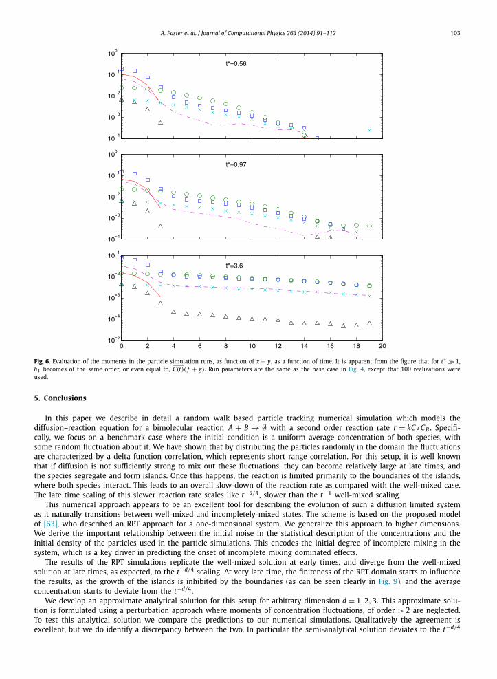
−h1(x, x, t) C(t)( f + g). In Fig. 6 we depict the dependence on distance of those moments, at some specific times in thesimulation. At later times we find −h1 C(t)( f + g), for all distances x − y. This result seems to explain the shift betweenthe analytical and numerical results observed in Fig. 4: recall that the analytical solution was obtained by neglecting thethird order moment h1 in (11). Because h1 < 0, neglecting it means that the C( f + g) + h1 term in (11) is over-estimatedin the analytical solution. Neglecting this term does not influence f − g , but does make f + g decay more quickly in (11),so the difference, −2g , is over-estimated. Because the late time balance is C √−g , this leads to an over-estimation of theaverage concentration given by the analytical solution, as depicted by the upshift seen in Fig. 4.

The effect of time discretization was tested for each simulation by running finer and finer time discretizations, and con-firming that changes in the results are negligible. We specifically test the effect of time discretization in terms of the valueof R = √

2DtN0/Ω . The results are shown in Fig. 7: as time discretization is refined and R gets smaller, the simulationresults are converging. The simulated average concentration differs by 0.1% from the converged value when R ∼ 1.4. Hence,if an error of 0.1% is considered acceptable, it is advised, as a rule of thumb, to use R ∼O(1). This implies that requirement(44) can be relaxed considerably.

4.2. Higher dimension

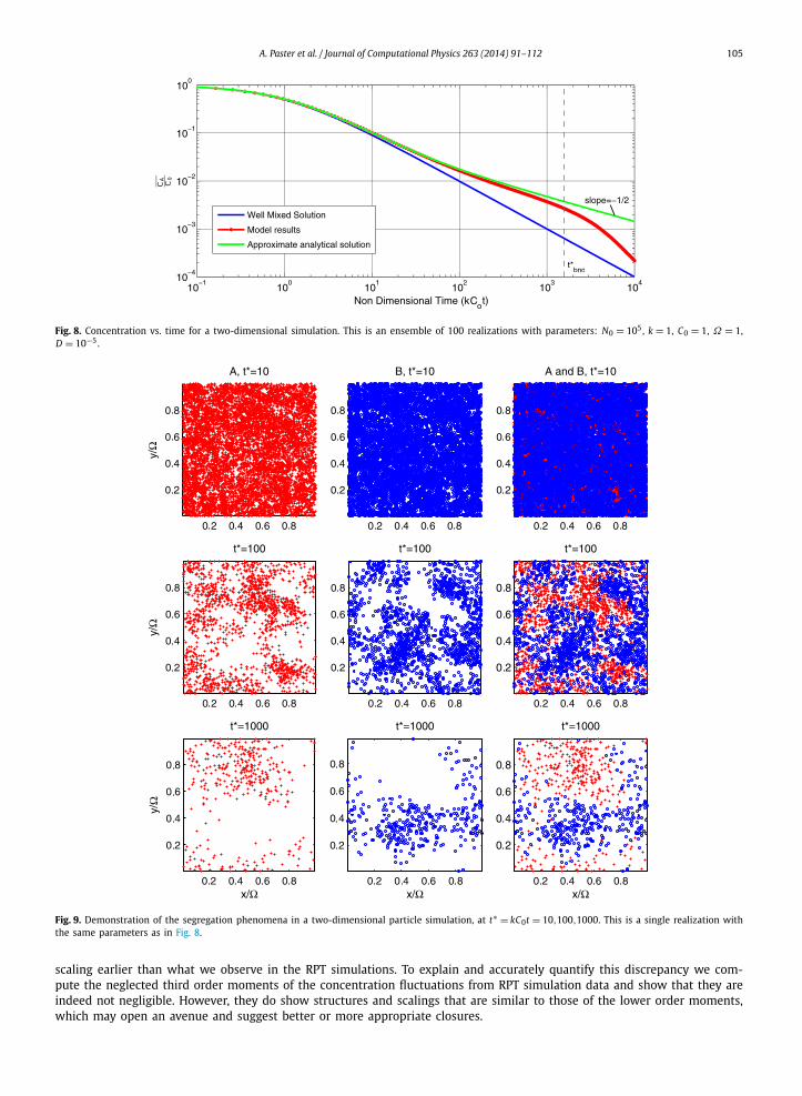
We also performed simulations in 2-d and 3-d systems. In Fig. 8 and Fig. 9, simulation results for a 2-d system areshown. As anticipated, both the simulation and analytical solution follow closely the t−1/2 curve. The breakdown from thiscurve at very late time occurs close to the non-dimensional time t∗

bnd = (1/64)kC0Ω2/D . This is consistent with the result

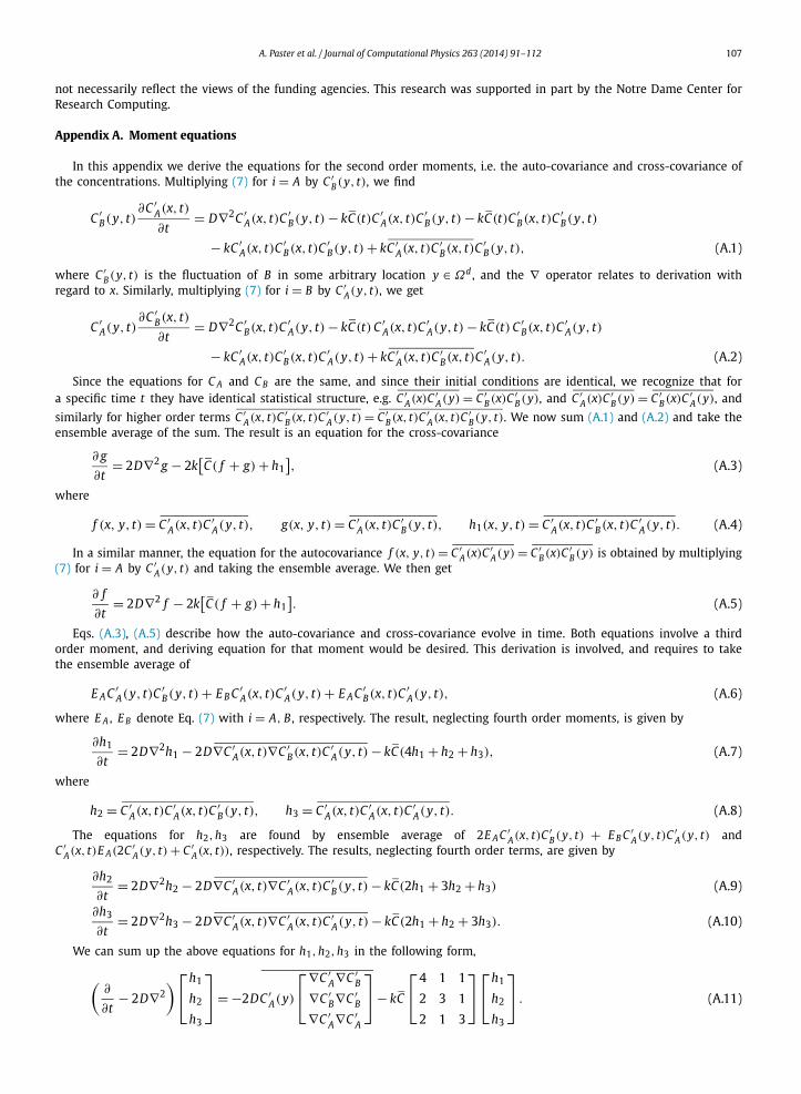
obtained by [17] for a one dimensional system. It is instructive to see, as depicted in Fig. 9, how the incomplete mixingregime develops at late times of the simulation (compare with Fig. 4(b)). Note the switch from the nearly well-mixed regimeat t∗ = 10 to a segregated domain in t∗ = 100, and note how the island size continues to grow at t∗ = 1000 ∼ t∗

bnd . At thistime, the islands growth is limited by the boundaries, since they cannot grow more then the size of the domain. Note howthe model results (Fig. 8) indeed start to deviate from the t−1/2 slope around this time.

Similar finding are obtained for 3-d systems. An example is given in Fig. 10, where we see that both the simulationand analytical solution follow closely the t−3/4 curve, and the breakdown occurs close to t∗

bnd . For illustration, in Fig. 10(b)we show a snapshot of a single realization at late time, when the system is highly segregated. The segregation we observein the two- and three-dimensional systems is in line with the results obtained by [5] and [18] and consistent with theobservations from 1-d for the same physical reasons.

The computational cost of the simulations, even in 3-d, is surprisingly low. We are unaware of an exact formula forthe duration of a simulation, because the number of particles at late time depends strongly on physical parameters (e.g.,a higher diffusion coefficient replicates better mixing and results in fewer particles at late time). However, for example, thetotal run time of the simulation used to produce Fig. 10(a) on the aforementioned PC, using 4 parallel computing nodes was0.8 h, i.e., 0.6 ms per initial A particle per realization.

A. Paster et al. / Journal of Computational Physics 263 (2014) 91–112 103

Fig. 6. Evaluation of the moments in the particle simulation runs, as function of x − y, as a function of time. It is apparent from the figure that for t∗ 1,h1 becomes of the same order, or even equal to, C(t)( f + g). Run parameters are the same as the base case in Fig. 4, except that 100 realizations wereused.

5. Conclusions

In this paper we describe in detail a random walk based particle tracking numerical simulation which models thediffusion–reaction equation for a bimolecular reaction A + B → ∅ with a second order reaction rate r = kC A C B . Specifi-cally, we focus on a benchmark case where the initial condition is a uniform average concentration of both species, withsome random fluctuation about it. We have shown that by distributing the particles randomly in the domain the fluctuationsare characterized by a delta-function correlation, which represents short-range correlation. For this setup, it is well knownthat if diffusion is not sufficiently strong to mix out these fluctuations, they can become relatively large at late times, andthe species segregate and form islands. Once this happens, the reaction is limited primarily to the boundaries of the islands,where both species interact. This leads to an overall slow-down of the reaction rate as compared with the well-mixed case.The late time scaling of this slower reaction rate scales like t−d/4, slower than the t−1 well-mixed scaling.

This numerical approach appears to be an excellent tool for describing the evolution of such a diffusion limited systemas it naturally transitions between well-mixed and incompletely-mixed states. The scheme is based on the proposed modelof [63], who described an RPT approach for a one-dimensional system. We generalize this approach to higher dimensions.We derive the important relationship between the initial noise in the statistical description of the concentrations and theinitial density of the particles used in the particle simulations. This encodes the initial degree of incomplete mixing in thesystem, which is a key driver in predicting the onset of incomplete mixing dominated effects.

The results of the RPT simulations replicate the well-mixed solution at early times, and diverge from the well-mixedsolution at late times, as expected, to the t−d/4 scaling. At very late time, the finiteness of the RPT domain starts to influencethe results, as the growth of the islands is inhibited by the boundaries (as can be seen clearly in Fig. 9), and the averageconcentration starts to deviate from the t−d/4.

We develop an approximate analytical solution for this setup for arbitrary dimension d = 1,2,3. This approximate solu-tion is formulated using a perturbation approach where moments of concentration fluctuations, of order > 2 are neglected.To test this analytical solution we compare the predictions to our numerical simulations. Qualitatively the agreement isexcellent, but we do identify a discrepancy between the two. In particular the semi-analytical solution deviates to the t−d/4

104 A. Paster et al. / Journal of Computational Physics 263 (2014) 91–112

Fig. 6. (continued)

Fig. 7. Smoothed cumulative density functions (CDF) of the concentration at time t = 1, for different time discretization, from coarse to fine (as the value ofR = √

2DtN0/Ω decreases). The vertical lines with respective color denote the mean of the realizations, C(t = 1). Note how the two finest discretizationspractically coincide, and are both within 0.1% tolerance of the solution by (15), C 0.506, denoted by a red vertical line. The parameters for those runsare: N0 = 103, D = 10−4, Ω = 1, C0 = 1, k = 1. Each CDF was evaluated based on 1000 realizations. Time was discretized into equally-long time steps;t = 0.1,0.033,0.01,0.001, respectively. Note that these curves fit closely to normal distribution, and that they have the same standard deviation (∼0.01).

A. Paster et al. / Journal of Computational Physics 263 (2014) 91–112 105

Fig. 8. Concentration vs. time for a two-dimensional simulation. This is an ensemble of 100 realizations with parameters: N0 = 105, k = 1, C0 = 1, Ω = 1,D = 10−5.

Fig. 9. Demonstration of the segregation phenomena in a two-dimensional particle simulation, at t∗ = kC0t = 10,100,1000. This is a single realization withthe same parameters as in Fig. 8.

scaling earlier than what we observe in the RPT simulations. To explain and accurately quantify this discrepancy we com-pute the neglected third order moments of the concentration fluctuations from RPT simulation data and show that they areindeed not negligible. However, they do show structures and scalings that are similar to those of the lower order moments,which may open an avenue and suggest better or more appropriate closures.

106 A. Paster et al. / Journal of Computational Physics 263 (2014) 91–112

Fig. 10. Results of a three-dimensional simulation. The model results are ensemble average of Nsim = 20 realizations with N0 = 256 000, Da =(kC0/D)Ω2/N2/d

0 = 22.3, d = 3. (a) Evolution of average concentration. (b) Illustration of interpolated C A along the domain boundaries at t∗ = kC0t = 100.

As with all numerical methods some numerical error will exist. There are several possible sources of error that wehave identified: first, the RPT simulations assume a cutoff distance δ (Eq. (30)), which means that we do not account forreactions between particles that are separated by a distance greater than this. The distance is chosen such that probabilityof reaction is minimal, but some error is introduced. Second, during the RPT simulations, when more than one of theB particles which neighbor an A particle have P f � U , only one of those B particles will be annihilated. The neglect ofthe other possible interactions may introduce some error. Third, errors might arise due to the chosen random numbergeneration, which is merely pseudo-random. Luckily all these errors can be minimized by using larger δ, smaller time step,and averaging over larger numbers of realizations, respectively. Thus, RPT simulations will converge to an accurate solutionof the diffusion–reaction equation, which we seek.

Acknowledgements

We thank the two anonymous reviewers for their valuable remarks on the manuscript. A.P. and D.B. would like toexpress thanks for financial support via Army Office of Research grant W911NF1310082 and NSF grant EAR-1113704. D.A.B.was supported by NSF grants DMS–0539176 and EAR–0749035. Any opinions, findings, conclusions, or recommendations do

A. Paster et al. / Journal of Computational Physics 263 (2014) 91–112 107

not necessarily reflect the views of the funding agencies. This research was supported in part by the Notre Dame Center forResearch Computing.

Appendix A. Moment equations

In this appendix we derive the equations for the second order moments, i.e. the auto-covariance and cross-covariance ofthe concentrations. Multiplying (7) for i = A by C ′

B(y, t), we find

C ′B(y, t)

∂C ′A(x, t)

∂t= D∇2C ′

A(x, t)C ′B(y, t) − kC(t)C ′

A(x, t)C ′B(y, t) − kC(t)C ′

B(x, t)C ′B(y, t)

− kC ′A(x, t)C ′

B(x, t)C ′B(y, t) + kC ′

A(x, t)C ′B(x, t)C ′

B(y, t), (A.1)

where C ′B(y, t) is the fluctuation of B in some arbitrary location y ∈ Ωd , and the ∇ operator relates to derivation with

regard to x. Similarly, multiplying (7) for i = B by C ′A(y, t), we get

C ′A(y, t)

∂C ′B(x, t)

∂t= D∇2C ′

B(x, t)C ′A(y, t) − kC(t) C ′

A(x, t)C ′A(y, t) − kC(t) C ′

B(x, t)C ′A(y, t)

− kC ′A(x, t)C ′

B(x, t)C ′A(y, t) + kC ′

A(x, t)C ′B(x, t)C ′

A(y, t). (A.2)

Since the equations for C A and C B are the same, and since their initial conditions are identical, we recognize that fora specific time t they have identical statistical structure, e.g. C ′

A(x)C ′A(y) = C ′

B(x)C ′B(y), and C ′

A(x)C ′B(y) = C ′

B(x)C ′A(y), and

similarly for higher order terms C ′A(x, t)C ′

B(x, t)C ′A(y, t) = C ′

B(x, t)C ′A(x, t)C ′

B(y, t). We now sum (A.1) and (A.2) and take theensemble average of the sum. The result is an equation for the cross-covariance

∂ g

∂t= 2D∇2 g − 2k

[C( f + g) + h1

], (A.3)

where

f (x, y, t) = C ′A(x, t)C ′

A(y, t), g(x, y, t) = C ′A(x, t)C ′

B(y, t), h1(x, y, t) = C ′A(x, t)C ′

B(x, t)C ′A(y, t). (A.4)

In a similar manner, the equation for the autocovariance f (x, y, t) = C ′A(x)C ′

A(y) = C ′B(x)C ′

B(y) is obtained by multiplying(7) for i = A by C ′

A(y, t) and taking the ensemble average. We then get

∂ f

∂t= 2D∇2 f − 2k

[C( f + g) + h1

]. (A.5)

Eqs. (A.3), (A.5) describe how the auto-covariance and cross-covariance evolve in time. Both equations involve a thirdorder moment, and deriving equation for that moment would be desired. This derivation is involved, and requires to takethe ensemble average of

E A C ′A(y, t)C ′

B(y, t) + E B C ′A(x, t)C ′

A(y, t) + E A C ′B(x, t)C ′

A(y, t), (A.6)

where E A , E B denote Eq. (7) with i = A, B , respectively. The result, neglecting fourth order moments, is given by

∂h1

∂t= 2D∇2h1 − 2D∇C ′

A(x, t)∇C ′B(x, t)C ′

A(y, t) − kC(4h1 + h2 + h3), (A.7)

where

h2 = C ′A(x, t)C ′

A(x, t)C ′B(y, t), h3 = C ′

A(x, t)C ′A(x, t)C ′

A(y, t). (A.8)

The equations for h2,h3 are found by ensemble average of 2E A C ′A(x, t)C ′

B(y, t) + E B C ′A(y, t)C ′

A(y, t) andC ′

A(x, t)E A(2C ′A(y, t) + C ′

A(x, t)), respectively. The results, neglecting fourth order terms, are given by

∂h2

∂t= 2D∇2h2 − 2D∇C ′

A(x, t)∇C ′A(x, t)C ′

B(y, t) − kC(2h1 + 3h2 + h3) (A.9)

∂h3

∂t= 2D∇2h3 − 2D∇C ′

A(x, t)∇C ′A(x, t)C ′

A(y, t) − kC(2h1 + h2 + 3h3). (A.10)

We can sum up the above equations for h1,h2,h3 in the following form,

(∂

∂t− 2D∇2

)⎡⎣h1

h2

⎤⎦ = −2DC ′

A(y)

⎡⎣∇C ′

A∇C ′B

∇C ′B∇C ′

B′ ′

⎤⎦ − kC

⎡⎣4 1 1

2 3 1

⎤⎦

⎡⎣h1

h2

⎤⎦ . (A.11)

h3 ∇C A∇C A 2 1 3 h3

108 A. Paster et al. / Journal of Computational Physics 263 (2014) 91–112

We can compute the eigenvectors and eigenvalues of the matrix on the RHS of (A.11), and use those to define combina-tions of (A.7)–(A.10),

H1 = 2h1 + h2 + h3, H2 = 2h1 − h2 − h3, H3 = 2h1 + 7h2 − 9h3. (A.12)

The equations for these combinations are

∂ H1

∂t= 2D∇2 H1 − 2D

(∇C ′A(x, t) + ∇C ′

B(x, t))2

C ′A(y, t) − 6kC H1,

∂ H2

∂t= 2D∇2 H2 − 2D

(∇C ′A(x, t) − ∇C ′

B(x, t))2

C ′A(y, t) − 2kC H2,

∂ H3

∂t= 2D∇2 H3 − 2DMC ′

A(y, t) − 2kC H3, (A.13)

where M = 2∇C ′A(x, t)∇C ′

B (x, t) + 7∇C ′B (x, t)∇C ′

B(x, t) − 9∇C ′A(x, t)∇C ′

A(x, t).

Appendix B. Numerical solution of the mean concentration

Eq. (15) can be decomposed into two coupled ODEs,⎧⎪⎪⎨⎪⎪⎩

dC

dt= −kC 2 − k

2

σ 2ld

(8π Dt)d/2

(−1 + e−4kγ ),

dγ

dt= C(t),

(B.1)

subject to initial conditions C(0) = C0, γ (0) = 0.This system cannot be solved straightforward, due to singularity that arises from the use of the delta function for the

initial condition. At t = 0+, the cross-covariance term in (B.1) tends to

g(x,y → x, t → 0+) ∼ 2σ 2ld

(8π D)d/2kC0t1−d/2. (B.2)

For d = 2, this is a constant; for d = 3, this tends to infinity. In both cases, the initial condition (12) is not satisfied. Howcan this contradiction be settled? Taking a step back, we note that (13) is the result of applying a diffusion operator overthe initial condition,

( f − g)(x,y, t) = L( f − g)(x,y, t = 0),

( f + g)(x,y, t) = L( f + g)(x,y, t = 0)exp

[−4k

t∫0

C(t′)dt′

], (B.3)

where Lϕ(x, . . .) = ∫ 1(8π Dt)d/2 exp[− (x−x′)2

8Dt ]ϕ(x′)dx′ is essentially a convolution of the initial condition by a Gaussian of

variance 4Dt . Subtracting these equations, and using g(x,y, t = 0) = 0, we would find

g(x,y, t) = 1

2L f (x,y, t = 0)

(−1 + exp

[−4k

t∫0

C(t′)dt′

]). (B.4)

Note that for the Delta function initial condition, the above result is exactly (13). Also, as t → 0+ , Eq. (B.4) tends tof (x,y, t = 0) × 2kC0t , and as long as the initial auto-correlation f is finite, this correctly converges to 0. The delta functionis a mathematical convenience we use instead of a physical initial condition, such as an exponentially decaying auto-correlation with small support. The critical difference between those is that physical initial conditions are finite everywhere,while the delta function is infinite at x = y. Thus, the solution with delta function initial condition is not valid at t → 0+ . Toresolve this, we assume g = 0 for a very short time, 0 < t � τ � (kC0)

−1. In other words, we assume a well-mixed solution(2) at the beginning of the simulation. With this assumption, the system evolves into

C(τ ) = C0

1 + kC0τ, γ (τ ) = 1

kln(1 + kC0τ ) ≈ C0τ . (B.5)

Because τ can be as small as we like, the error introduced by this assumption is negligible, as long as τ is chosen tobe a few orders of magnitude smaller than (kC0)

−1, the typical time of reaction. Now we solve numerically the coupledODEs (B.1), subject to initial condition (B.5), by standard numerical tools for stiff systems (e.g. [69]). It is also possible toovercome the singularity in (B.1) by using an asymptotic formula for short times [45]. The results are similar to the oneswe obtain here.

A. Paster et al. / Journal of Computational Physics 263 (2014) 91–112 109

Appendix C. Cross-covariance for numerical particle method

C.1. General

The goal of this appendix is to calculate the initial cross-covariance of the concentration that is presumably describedby the particles in the particle method. This is crucial in order to be able to compare this initial cross-covariance with theone assumed for the analytically derived solution of the Diffusion-Reaction equation (1), and to be able to compare the twoapproaches.

Our basic postulation is that a continuous property in a domain Ωd (such as concentration, C(x, t), which we discusshere) can be approximately represented by a particle system with N0 particles whose location is given by Xi(t) ∈ Ωd , where1 � i � N0. We assume that each particle represents a constant mass mp . Clearly, if chemical reactions are involved, thenumber of particles N0 depends on time. The basic concept of the particle method lies in the way the concentration, whichis a continuous property, is described by the particle locations. One way of evaluating the concentration is by “smearing” themass of each particle around its given location by a weight function, then summing up the contributions of all the particlesin a given point x. We have derived the cross-covariance for two choices of weighting function: (I) a delta weightingfunction, and (II) a Gaussian weighting function. Both results will be shown in this appendix. The use of delta function isjustified by the fact we regard a specific particle system as a single realization of a stochastic system and thus the physicalmeaning is given by ensemble average over infinite number of such realizations. Such ensemble average yields the desiredsmooth concentration. For the delta weighting function, the estimated concentration in a certain location is given by

C p(x, t) =N0∑

i=1

mpδ(x − Xi), (C.1)

where the subscript p stands for particle estimation (in contrast to the actual value).The total mass in the system is given by mp N0 and the average concentration is given by

C p = 1

Ωd

∫Ωd

C p(x, t)dx = mp N0

Ωd. (C.2)

The fluctuation over the mean is given by C ′p(x, t) = C p(x, t) − C p(t) and the cross-covariance of the particle concentra-

tion is defined as the ensemble average of all possible particle location “scenarios”, i.e.

C ′p(x)C ′

p(y) =∫

Ωd

· · ·∫

Ωd

C ′p(x)C ′

p(y) f (X1, . . . ,XN0)dX1 · · · dXN0 , (C.3)

where f (X1, . . . ,XN0 ) is the joint p.d.f. of the particle locations. Note that the integration is performed N times.

C.2. Evaluation of cross-covariance

Next, we assume that N0 particles were randomly spread in the domain and would like to evaluate the cross-covariance (C.3). We write (C.3) as

C ′p(x)C ′

p(y) = C p(x)C p(y) − C p2, (C.4)

and the second term on the RHS is known from (C.2), so we shall focus on evaluating the first term . Using (C.1)

C p(x)C p(y) = m2p

∫Ωd

· · ·∫

Ωd

N0∑i=1

δ(x − Xi)

N0∑j=1

δ(y − X j) f (X1, . . . ,XN0)dX1 · · · dXN0 . (C.5)

The above expression simplifies significantly in our case. First, our particles are spread randomly in the domain, so the p.d.f.of each of them equals Ω−d . Second, they are independent, so the joint p.d.f. is f (X1, . . . ,XN0) = f (X1) f (X2) · · · f (XN0 ) =Ω−N0d . Third, we can change the order of summation and integration, and write (6) as

C p(x)C p(y) = m2p

N0∑i=1

N0∑j=1

Ii j, (C.6)

where

Ii j =∫

d

· · ·∫

d

δ(x − Xi)δ(y − X j)Ω−N0d dX1 · · · dXN0 . (C.7)

Ω Ω

110 A. Paster et al. / Journal of Computational Physics 263 (2014) 91–112

We shall first examine the case i �= j. Since Ii j is independent of all X, except Xi,X j , it can be reduced to

Ii j = Ω−2d∫

Ωd

δ(x − Xi)dXi

∫Ωd

δ(y − X j)dX j = Ω−2d. (C.8)

We have N0(N0 − 1) such terms, where i �= j, so their total contribution in (C.6) is

m2p N0(N0 − 1)Ω−2d. (C.9)

Next we turn to look at the i = j case. Reducing (C.7) by N0 − 1 integrations we get

Iii = Ω−d∫

Ωd

δ(x − Xi)δ(y − Xi)dXi = Ω−dδ(x − y). (C.10)

There are N0 such terms, and thus their total contribution in (C.6) is

m2p N0Ω

−dδ(x − y). (C.11)

Summing up the contributions (C.11) and (C.9) we find

C p(x)C p(y) = m2p N0

[Ω−dδ(x − y) + (N0 − 1)Ω−2d]. (C.12)

Substituting this result, together with (C.2), into (C.4), we get the final result for the non-dimensional auto-covariance

C ′p(x)C ′

p(y)

C p2

= Ωd

N0δ(x − y) − 1

N0. (C.13)

We shall now discuss this result. Looking at the expression in (C.13) we can see it consists of two terms: a delta functionterm, and a −1/N0 term. In fact, this expression somewhat resembles the initial condition assigned to the correlationdiscussed in the derivation of the analytical solution (19). The difference lies in the factor in front of the delta function, andin the existence of the −1/N0 term, not considered in the analytical approach. This second term can be understood in thefollowing way: the fact that the concentration in a certain point is high, means that we are “sitting” on a particle, i.e. in theclose vicinity of it. If this is so, the concentration far away from the current location is made of N0 − 1 particles. Thus, it islower then the average, and we have a negative auto-covariance there, described by the −1/N0 term. In order to even betterunderstand the result, we can derive the auto-covariance (C.4) once more, however this time considering a Gaussian weightfunction, instead of the delta function in (C.1). To accomplish this, we have to define some small volume scale, hd , whichrepresents the support of the particle. It makes sense then to choose some value that will be about the order of Ωd/N0, thetotal volume divided by the number of particles. Simply choosing hd = Ωd/N0, and assigning the Gaussian weight functionto each particle, the estimated concentration for the one-dimensional case is approximately given by

C p(x, t) �N0∑

i=1

mp√2πh2

exp

[− (x − Xi(t))2

2h2

]. (C.14)

In order to make this expression exact, we need to take into account an infinite number of image particles in the adjacentdomains. Fortunately, for the small particle support considered here, the approximate expression (C.14) is still accurate,except at regions close to the boundaries of the domain. Now, if we derive the auto-covariance (C.4), along the same linesas delineated by equations (C.5)–(C.13), however using the Gaussian weight function, we obtain

C ′p(x)C ′

p(y)

C p2

= 1

N0

[Ω√

4πh2exp

[− (x − y)2

4h2

]− 1

]. (C.15)

Substituting h = Ω/N0 in (C.15) we get

C ′p(x)C ′

p(y)

C p2

= 1√4π

exp

[− (x − y)2

4h2

]− 1

N0. (C.16)

This result, in fact, can be easily ascertained by numerical simulations. The expression in (C.16) resembles (C.13), exceptthat the delta function was replaced by a Gaussian with variance 2h2. Moreover, for the auto-covariance, i.e. for x = y, wefind that the contribution of the −1/N0 term is practically negligible, since particle numerical simulations have typically avery large number of particles for the sake of a statistical meaningful result. Along the same lines, the −1/N0 term in (C.13)is negligible, and

C ′p(x)C ′

p(y) C20Ωd

N0δ(x − y). (C.17)

This result may serve in understanding the evolution of a system of such random particles, when the system state isdependent on the initial conditions.

A. Paster et al. / Journal of Computational Physics 263 (2014) 91–112 111

References

[1] E. Kotomin, V. Kuzovkov, Modern Aspects of Diffusion-Controlled Reactions: Cooperative Phenomena in Bimolecular Processes, Comprehensive ChemicalKinetics, Elsevier, 1996.

[2] A. Ovchinnikov, Y. Zeldovich, Role of density fluctuations in bimolecular reaction kinetics, Chem. Phys. 28 (1–2) (1978) 215–218, http://dx.doi.org/10.1016/0301-0104(78)85052-6.

[3] S. Rice, Diffusion-Limited Reactions, Comprehensive Chemical Kinetics, Elsevier, 1985.[4] K. Kang, S. Redner, Scaling approach for the kinetics of recombination processes, Phys. Rev. Lett. 52 (1984) 955.[5] D. Toussaint, F. Wilczek, Particle–antiparticle annihilation in diffusive motion, J. Chem. Phys. 78 (1983) 2642–2647.[6] J. Murray, Mathematical Biology: I. An Introduction, vol. 2, Springer, 2002.[7] J. Fort, V. Méndez, Reaction–diffusion waves of advance in the transition to agricultural economics, Phys. Rev. E 60 (5) (1999) 5894–5901.[8] D. Becherer, M. Schweizer, Classical solutions to reaction–diffusion systems for hedging problems with interacting Itô and point processes, Ann. Appl.

Probab. 15 (2) (2005) 1111–1144.[9] C.-Z. Li, K.-G. Löfgren, Renewable resources and economic sustainability: a dynamic analysis with heterogeneous time preferences, J. Environ. Econ.

Manag. 40 (3) (2000) 236–250.[10] F. Schweitzer, Brownian Agents and Active Particles: Collective Dynamics in the Natural and Social Sciences, Springer, 2007.[11] A.A. Keller, Reaction–diffusion systems in natural sciences and new technology transfer, J. Mech. Behav. Mater. 21 (2012) 123–146.[12] M.A. Fields, Modeling large scale troop movement using reaction diffusion equations, Tech. rep., DTIC Document, 1993.[13] R.S. Cantrell, C. Cosner, Spatial Ecology via Reaction–Diffusion Equations, Wiley, 2004.[14] D. Gillespie, The chemical Langevin equation, J. Chem. Phys. 113 (1) (2000) 297–306.[15] A. Kudryavtsev, R.F. Jameson, W. Linert, The Law of Mass Action, Springer-Verlag, 2001.[16] S. Havlin, D. Ben-Avraham, Diffusion in disordered media, Adv. Phys. 36 (6) (1987) 695–798.[17] D. Bolster, P. de Anna, D.A. Benson, A.M. Tartakovsky, Incomplete mixing and reactions with fractional dispersion, Adv. Water Resour. 37 (2012) 86–93,

http://dx.doi.org/10.1016/j.advwatres.2011.11.005.[18] G. Zumofen, J. Klafter, M. Schlesinger, Breakdown of Ovchinnikov–Zeldovich segregation in the A + B → 0 reaction under Lévy mixing, Phys. Rev. Lett.

77 (1996) 2830–2833.[19] A. Lin, R. Kopelman, P. Argrakis, Nonclassical kinetics in three dimensions: Simulations of elementary A + B and A + A reactions, Phys. Rev. E 53 (1996)

1502–1509.[20] P. de Anna, T.L. Borgne, M. Dentz, D. Bolster, P. Davy, Anomalous kinetics in diffusion limited reactions linked to non-Gaussian concentration probability

distribution function, J. Chem. Phys. 135 (17) (2011) 174104, http://dx.doi.org/10.1063/1.3655895.[21] G. Oshanin, I.M. Sokolov, P. Argyrakis, A. Blumen, Fluctuation-dominated A + B → 0 kinetics under short-ranged interparticle interactions, J. Chem.

Phys. 105 (15) (1996) 6304–6314, http://dx.doi.org/10.1063/1.472466.[22] E. Monson, R. Kopelman, Observation of laser speckle effects and nonclassical kinetics in an elementary chemical reaction, Phys. Rev. E 85 (2000)

666–669.[23] E. Monson, R. Kopelman, Nonclassical kinetics of an elementary A + B → C reaction–diffusion system showing effects of a speckled initial reactant

distribution and eventual self-segregation: Experiments, Phys. Rev. E 69 (2004) 021103.[24] D.S. Raje, V. Kapoor, Experimental study of bimolecular reaction kinetics in porous media, Environ. Sci. Technol. 34 (7) (2002) 1234–1239, http://

dx.doi.org/10.1021/es9908669.[25] C. Gramling, C. Harvey, L. Meigs, Reactive transport in porous media: a comparison of model prediction with laboratory visualization, Environ. Sci.

Technol. 36 (2002) 2508–2514, http://dx.doi.org/10.1021/es0157144.[26] J. Hill, Homogeneous turbulent mixing with chemical-reaction, Annu. Rev. Fluid Mech. 8 (1976) 135–161, http://dx.doi.org/10.1146/annurev.fl.

08.010176.001031.[27] C.d. Donaldson, G.R. Hilst, Effect of inhomogeneous mixing on atmospheric photochemical reactions, Environ. Sci. Technol. 6 (9) (1972) 812–816.[28] R. Sullivan, M. Moore, M. Petters, S. Kreidenweis, G. Roberts, K. Prather, Effect of chemical mixing state on the hygroscopicity and cloud nucleation

properties of calcium mineral dust particles, Atmos. Chem. Phys. 9 (10) (2009) 3303–3316.[29] Y. Salomon, S.R. Connolly, L. Bode, Effects of asymmetric dispersal on the coexistence of competing species, Ecol. Lett. 13 (4) (2010) 432–441.[30] T. LeBorgne, M. Dentz, P. Davy, D. Bolster, J. Carrera, J. deDreuzy, O. Bour, Persistence of incomplete mixing: A key to anomalous transport, Phys. Rev. E

84 (2011) 15301.[31] T. LeBorgne, M. Dentz, D. Bolster, J. Carrera, J. deDreuzy, P. Davy, Non-Fickian mixing: temporal evolution of the scalar dissipation rate in porous media,

Adv. Water Resour. 33 (2010) 1468–1475.[32] F. de Barros, M. Dentz, J. Koch, W. Nowak, Flow topology and scalar mixing in spatially heterogeneous flow fields, Geophys. Res. Lett. 39 (2012) L08404.[33] O. Gorodetskyi, M. Speetjens, P. Anderson, An efficient approach for eigenmode analysis of transient distributive mixing by the mapping method, Phys.

Fluids 24 (2012) 053602.[34] E. Castro-Alcalà, D. Fernández-Garcia, J. Carrera, D. Bolster, Visualization of mixing processes in a heterogeneous sand box aquifer, Environ. Sci. Technol.

46 (6) (2012) 3228–3235.[35] D. Bolster, F.J. Valdés-Parada, T. LeBorgne, M. Dentz, J. Carrera, Mixing in confined stratified aquifers, J. Contam. Hydrol. 120 (2011) 198–212.[36] A. Klimenko, Mixing, entropy and competition, Phys. Scr. 85 (6) (2012) 068201.[37] A.M. Tartakovsky, D.M. Tartakovsky, P. Meakin, Stochastic Langevin model for flow and transport in porous media, Phys. Rev. Lett. 101 (2008) 044502.[38] A.M. Tartakovsky, Langevin model for reactive transport in porous media, Phys. Rev. E 82 (2010) 026302.[39] Y. Edery, H. Scher, B. Berkowitz, Modeling bimolecular reactions and transport in porous media, Geophys. Res. Lett. 36 (2009) L02407.[40] J.R. Bourne, Mixing and the selectivity of chemical reactions, Org. Process Res. Dev. 7 (4) (2003) 471–508.[41] C. Meile, K. Tuncay, Scale dependence of reaction rates in porous media, Adv. Water Resour. 29 (1) (2006) 62–71, http://dx.doi.org/10.1016/

j.advwatres.2005.05.007.[42] L.D. Donado, X. Sanchez-Vila, M. Dentz, J. Carrera, D. Bolster, Multicomponent reactive transport in multicontinuum media, Water Resour. Res. 45 (11)

(2009) W11402.[43] D. Bolster, D.A. Benson, T. Le Borgne, M. Dentz, Anomalous mixing and reaction induced by superdiffusive nonlocal transport, Phys. Rev. E 82 (2) (2010)

021119, http://dx.doi.org/10.1103/PhysRevE.82.021119.[44] J. Wang, Stirring-induced oscillations in an excitable chemical system with inhomogeneous reaction dynamics, J. Phys. Chem. A 107 (41) (2003)

8774–8778.[45] A.M. Tartakovsky, P. de Anna, T.L. Borgne, A. Balter, D. Bolster, Effect of spatial concentration fluctuations on effective kinetics in diffusion–reaction

systems, Water Resour. Res. 48 (2012) W02526, http://dx.doi.org/10.1029/2011WR010720.[46] A. Paster, D. Bolster, The effect of initial spatial correlations on late time kinetics of bimolecular irreversible reactions, Phys. A, Stat. Mech. Appl.

391 (20) (2012) 4654–4660.[47] J. Lipková, K. Zygalakis, S. Chapman, R. Erban, Analysis of Brownian dynamics simulations of reversible bimolecular reactions, SIAM J. Appl. Math. 71 (3)

(2011) 714–730, http://dx.doi.org/10.1137/100794213.

112 A. Paster et al. / Journal of Computational Physics 263 (2014) 91–112

[48] M. von Smoluchowski, Versuch einer mathematischen theorie der koagulationskinetik kolloider lösungen, Z. Phys. Chem. 92 (1917) 124–168.[49] M. Doi, Stochastic theory of diffusion-controlled reaction, J. Phys. A, Math. Gen. 9 (1976) 1479–1495.[50] K. Kang, S. Redner, Fluctuation-dominated kinetics in diffusion-controlled reactions, Phys. Rev. A 32 (1985) 435–447.[51] B. Chopard, M. Droz, Microscopic study of the properties of the reaction front in an A + B → C reaction–diffusion process, Europhys. Lett. 15 (4) (1991)

459.[52] A.F.B. Tompson, D.E. Dougherty, Particle-grid methods for reacting flows in porous media with application to Fisher’s equation, Appl. Math. Model. 16

(1992) 374–383.[53] D. Bernstein, Simulating mesoscopic reaction–diffusion systems using the Gillespie algorithm, Phys. Rev. E 71 (2005) 041103, http://dx.doi.org/10.1103/

PhysRevE.71.041103.[54] S.A. Isaacson, A convergent reaction–diffusion master equation, J. Chem. Phys. 139 (5) (2013) 054101, http://dx.doi.org/10.1063/1.4816377.[55] A. Einstein, Über die von der molekularkinetischen theorie der wärme geforderte bewegung von in ruhenden flüssigkeiten suspendierten teilchen, Ann.

Phys. 322 (8) (1905) 549–560, http://dx.doi.org/10.1002/andp.19053220806.[56] S. Chandrasekhar, Stochastic problems in physics and astronomy, Rev. Mod. Phys. 15 (1943) 1–89, http://dx.doi.org/10.1103/RevModPhys.15.1.[57] H. Risken, The Fokker–Planck Equation: Methods of Solution and Applications, Springer-Verlag, 1984.[58] W. Kinzelbach, The random walk method in pollutant transport simulation, in: E. Custodio, A. Gurgui, J.L. Ferreira (Eds.), Groundwater Flow and Quality

Modelling, in: NATO Adv. Stud. Inst. Ser., Ser. C, Math. Phys. Sci., vol. 224, 1988, pp. 227–245.[59] T. Prickett, T. Naymik, C. Lonnquist, A “random-walk” solute transport model for selected groundwater quality evaluations, in: Bulletin, vol. 65, Illinois

State Water Survey, Champaign, IL, 1981.[60] A.S. Sherman, C.S. Peskin, A Monte Carlo method for scalar reaction diffusion equations, SIAM J. Sci. Stat. Comput. 7 (4) (1986) 1360–1372.[61] R.A. Kerr, T.M. Bartol, B. Kaminsky, M. Dittrich, J.-C.J. Chang, S.B. Baden, T.J. Sejnowski, J.R. Stiles, Fast Monte Carlo simulation methods for biological

reaction–diffusion systems in solution and on surfaces, SIAM J. Sci. Comput. 30 (6) (2008) 3126–3149.[62] Y. Zhang, C. Papelis, Particle-tracking simulation of fractional diffusion–reaction processes, Phys. Rev. E 84 (2011) 066704, http://dx.doi.org/10.1103/

PhysRevE.84.066704.[63] D.A. Benson, M.M. Meerschaert, Simulation of chemical reaction via particle tracking: Diffusion-limited versus thermodynamic rate-limited regimes,

Water Resour. Res. 44 (2008) W12201, http://dx.doi.org/10.1029/2008WR007111.[64] A. Paster, D. Bolster, D.A. Benson, Particle tracking and the diffusion–reaction equation, Water Resour. Res. 49 (2013) 1–6, http://dx.doi.org/10.1029/

2012WR012444.[65] J.S. van Zon, P.R. ten Wolde, Simulating biochemical networks at the particle level and in time and space: Green’s function reaction dynamics, Phys.

Rev. Lett. 94 (12) (2005) 128103.[66] D. Ding, D.A. Benson, A. Paster, D. Bolster, Modeling bimolecular reactions and transport in porous media via particle tracking, Adv. Water Resour. 53

(2013) 56–65, http://dx.doi.org/10.1016/j.advwatres.2012.11.001.[67] M. De Berg, O. Cheong, M. Van Kreveld, M. Overmars, Computational Geometry: Algorithms and Applications, Springer, 2008.[68] D. Fernàndez-Garcia, X. Sanchez-Vila, Optimal reconstruction of concentrations, gradients and reaction rates from particle distributions, J. Contam.

Hydrol. 120 (2011) 99–114.[69] C. Pozrikidis, Numerical Computation in Science and Engineering, 2nd edition, Oxford University Press, 2008.