Analysis Program - seas.upenn.edualur/CIS670/sriram1.pdfWhat is Abstract In terpretation? F ormal...
44
Transcript of Analysis Program - seas.upenn.edualur/CIS670/sriram1.pdfWhat is Abstract In terpretation? F ormal...

CIS 670: Program Analysis
Title: Abstra t Interpretation.Guest Le turer: Sriram Sankaranarayanan.NEC Labs Ameri a,Prin eton, NJ.srirams�ne -labs. omDate: O t 1st, 2007.1

Topi s
� Programs, Flow harts, et ...� Instan es of Abstra t Interpretation:� Analysis #1: Sign Analysis.� Analysis #2: Interval Analysis.� �Con rete� Interpretation.� Abstra t Interpretation.2

What is Abstra t Interpretation?
Formal study of �xed points for program analysis appli ations.� Program Veri� ation Appli ations:Astrée, PolySpa e, CoVerity, Absinthe, F-Soft,CodeSurfer, Flu tuat, Aira , TVLA, ...� Denotational Semanti s.� Type Che king/Inferen e.3

Goals
� There are numerous presentations of abstra t interpretation.
� Our goal:1. Today: Understand the essen e of the theory(without too mu h �Greek�).2. Today & Wednesday: The a tual theory.3. Wednesday: A qui k guided tour through importantappli ations & resear h frontiers.� Will try to be self- ontained as mu h as possible.
4

Some History� Theory of indu tive invariants: [Floyd, 1967℄ and [Hoare, 1969℄.� Denotational Semanti s: [S ott, Reynolds, Abramsky, ...℄� Invariant Generation: [King, 1969; Manna & Katz, 1975℄� Monotone frameworks for data�ow analysis: [Burstall, 1973℄.� Linear equality invariant generation: [Karr, 1976℄� Interval analysis: [Cousot & Cousot, 1976℄� Abstra t interpretation theory: [Cousot&Cousot, 1977℄� Polyhedral Analysis: [Cousot & Halbwa hs, 1978℄� Re ent advan es & appli ations.5

Programs
We will use a standard �ow hart representation.fun tion foo ( int x )int y := x ∗ x + 1 ;while y > 1 doif y%2 == 0 theny = y/2else
y = 3 ∗ y + 1end ifend whileend fun tionn0: y := x ∗ x + 1
n1: +
n2: y > 1
n3: y%2 == 0
n4: y := y/2 y := 3y + 1
n5: +
6

Program: Assumptions
For simpli ity, we make the following assumptions about ourprograms:� All variables are integers or reals.� No fun tion alls.� No pointers, arrays, ompound obje ts.Note: Real program analysis tools handle features su h asfun tion alls, arrays, pointers and ompound stru tures.
7

Signs Analysis
For ea h lo ation n,For ea h variable x,sign(n, x) =
‘‘⊥ ′′ if ontrol never rea hes n
‘‘+ ′′, if x > 0, whenever ontrol rea hes n,
‘‘− ′′ if x < 0, · · ·
‘‘0 ′′ if x = 0, · · ·
‘‘⊤ ′′ otherwise8

Signs Latti eThe symbols {⊥, +, −, 0,⊤} orrespond to the sets of naturalnumbers:[[⊥]] : ∅ [[⊤]] : Z
[[+]] : {x|x > 0} [[−]] : {x|x < 0}Sets of natural numbers an be ordered by in lusion ⊆.
Z ⊤
{x|x > 0} {0} {x|x < 0} + 0 -∅ ⊥
⊆ ⊑
The ⊆ indu es a ⊑ relation in the sign domain.9

Signs Analysis: Problem Statement
For ea h variable x, and ea h lo ation n omputethe least element of the signs latti e c su h that
[[c]] ontains all the possible values of x seen when ontrol rea hes lo ation n.10

Signs Analysis: Least Solution
Assume input state sign(x, n0) : +, sign(y, n0) : ⊤.Flow hart sign(y, n) sign(x, n)
n0: y := x ∗ x + 1 ⊤ +
n1: + +
n2: y > 1 + +
n3: y%2 == 0 + +
n4: y := y/2 y := 3y + 1 + +
n5: + +11

Signs Analysis: Problem Statement (Attempt # 2)
For ea h variable x, and ea h lo ation n omputethe least element some element of the signs latti e
c su h that [[c]] ontains all the possible values of
x seen when ontrol rea hes lo ation n.� Least element of the latti e annot be omputed.Proof: Redu e from Hilbert's 10th problem.� Trivial analysis result: sign(n, x) : ⊤ at all lo ations!!� Least solution in the latti e.1. Derive latti e inequalities for the overapproximations.2. Solve them to derive a safe overapproximation.
12

Signs Analysis: Data-�ow equations
n0 : y := · · · post(n0, sign(n0, x)) ⊑ sign(n1, y)
n1 sign(n5, y) ⊑ sign(n1, y)
n2 : y > 1 sign(n1, y) ⊑ sign(n2, y)
n3 : ϕ1 sign(n2, y) ⊓ α([[y > 1]]) ⊑ sign(n3, y)
n4 : · · · n6 : · · · sign(n3, y) ⊓ α([[ϕ1]]) ⊑ sign(n4, y)
n5 post(n4, sign(n4, y)) ⊑ sign(n5, y)
post(n6, sign(n6, y)) ⊑ sign(n5, y)
13

Abstra tionGiven a set of integers I , α(I) is the smallest value in the signlatti e that overs it.α(I)
∆= min⊑{c ∈ sign|[[c]] ⊇ I} .Example:
I α(I)
{x|x > 10} +
{x|x <= 1} ⊤
{x|x <= 0} ⊤
{x|x < 0} −
∅ ⊥
14

Signs Analysis: Post-Condition
Consider an assignment y := expr(x1, . . . , xn).Post: Given the sign values of x1, . . . , xn before an assignment, ompute the sign value of y after the assignment.
post(n : y := expr, 〈sign(n, x1), . . . , sign(n, xn)〉) .Example: Consider assignment n0 : y := x ∗ x + 1
x ⊥ + 0 − ⊤
post(y := · · · , sign(n, x)) ⊥ + + + +
15

Computing post onditionGoal: Compute post(y := expr, 〈sign(n, x0), . . . , sign(n, xm)〉).
Just �follow� the expression syntax.Example: Let expr : y − z − x + 1 and〈sign(n, x) : ‘‘0 ′′, sign(n, y) : ‘‘− ′′, sign(n, z) : ‘‘+ ′′〉.
1. p(y − z) = p(‘‘ − ′′ −‘‘+ ′′) = ‘‘− ′′
2. p((y − z) − x) = p(‘‘ − ′′ −‘‘0 ′′) = ‘‘− ′′
3. p(((y − z) − x) + 1) = p(‘‘ − ′′ +‘‘+ ′′) = ‘‘⊤ ′′
∴ post(expr, 〈sign(n, x) : ‘‘0 ′′, sign(n, y) : ‘‘− ′′, sign(n, z) : ‘‘+ ′′〉) = ⊤ .
16

Post ondition: ExampleAssignment n0 : y := x ∗ x + 1.
x ⊥ + 0 − ⊤
post(y := · · · , sign(n, x)) ⊥ + + + +Assignment n4 : y := 3 ∗ y + 1.y ⊥ + 0 − ⊤
post(y := · · · , sign(n, y)) ⊥ + + − ⊤Assignment n6 : y := y/2.y ⊥ + 0 − ⊤
post(y := · · · , sign(n, y)) ⊥ ⊤ 0 ⊤ ⊤
17

Latti es, Monotoni Fun tions & Fixed Points
Poset: A set L with a partial order ⊑.
Meet & Join:a ⊓ b = max⊑{c|c ⊑ a, c ⊑ b}
a ⊔ b = min⊑{c|a ⊑ c, b ⊑ c}Latti e: Meets and Joins exists for every pair a, b.(Therefore, meet and join exists every �nite subset)Complete Latti e: Every subset has a meet and a join.(related on ept: semi- omplete latti e).18

Monotone fun tion: f : L 7→ L, s.t. a ⊑ b ⇒ f(a) ⊑ f(b).Fixed Point: a = f(a).Theorem: [Knaster, 1928; Tarski, 1953℄
Every monotone fun tion on a omplete latti e hasa least and greatest �xed point.Proof:
LFP(f) : max⊑(⊥, f(⊥), f2(⊥), . . . , )
GFP(f) : min⊑(⊤, f(⊤), f2(⊤), . . . , )
19

Signs Analysis: Data-�ow equations
n0 : y := · · · post(n0, sign(n0, x)) ⊑ sign(n1, y)
n1 sign(n5, y) ⊑ sign(n1, y)
n2 : y > 1 sign(n1, y) ⊑ sign(n2, y)
n3 : ϕ1 sign(n2, y) ⊓ ‘‘+ ′′ ⊑ sign(n3, y)
n4 : · · · n6 : · · · sign(n3, y) ⊓ ‘‘⊤ ′′ ⊑ sign(n4, y)
n5 post(n4, sign(n4, y)) ⊑ sign(n5, y)
post(n6, sign(n6, y)) ⊑ sign(n5, y)20

Signs Analysis: Data-�ow equations
‘‘⊤ ′′ ⊑ sign(n0, y)
post(n0, sign(n0, x)) ⊔ sign(n5, y) ⊑ sign(n1, y)
sign(n1, y) ⊑ sign(n2, y)
sign(n2, y) ⊓ ‘‘+ ′′ ⊑ sign(n3, y)
sign(n3, y) ⊓ ‘‘⊤ ′′ ⊑ sign(n4, y)
post(n4, sign(n4, y)) ⊔ post(n6, sign(n6, y)) ⊑ sign(n5, y)
‘‘+ ′′ ⊑ sign(n0, x)
sign(n0, x) ⊔ sign(n5, x) ⊑ sign(n1, x)
sign(n1, x) ⊑ sign(n2, x)...sign(n4, x) ⊔ sign(n6, x) ⊑ sign(n5, x)21

Shorthand notation: xi : sign(ni, x) and yi : sign(ni, y).We may write the (in)equalities as :
f1(x1, . . . , xn, y1, . . . , yn) ⊑ y1...
fn(x1, . . . , xn, y1, . . . , yn) ⊑ yn
g1(x1, . . . , xn, y1, . . . , yn) ⊑ x1...gn(x1, . . . , xn, y1, . . . , yn) ⊑ xn
22

Inequations over a latti e
Let L be a latti e and f1, . . . , fn be monotoni fun tions:
fj : L × · · · × L 7→ L .Corollary Knaster-Tarski Theorem: The inequality system
f1(x1, . . . , xn) ⊑ x1, f2(x1, . . . , xn) ⊑ x2, · · · , fn(x1, . . . , xn) ⊑ xn .has a smallest and a greatest solution.Furthermore, these solutions will satisfy:f1(x1, . . . , xn) = x1, . . . , fn(x1, . . . , xn) = xn .Proof: · · ·
23

Solving inequations over a latti eCompute least solution for the latti e inequality system
f1(x1, . . . , xn) ⊑ x1, f2(x1, . . . , xn) ⊑ x2, · · · , fn(x1, . . . , xn) ⊑ xn .Initial solution: x01 = ⊥, . . . , x0
n = ⊥.
Iterative step:xi+1
1 = f1(xi1, xi
2, . . . , xin),...
xi+1n = fn(xi
1, xi2, . . . , xi
n) .Stopping riteria: (∀ j ∈ [1, n]) xi+1j ⊑ xi
j.24

Che k that LHS fun tions are monotoni :
‘‘⊤ ′′ ⊑ sign(n0, y)
post(n0, sign(n0, x)) ⊔ sign(n5, y) ⊑ sign(n1, y)
sign(n1, y) ⊑ sign(n2, y)
sign(n2, y) ⊓ ‘‘+ ′′ ⊑ sign(n3, y)
sign(n3, y) ⊓ ‘‘⊤ ′′ ⊑ sign(n4, y)
post(n4, sign(n4, y)) ⊔ post(n6, sign(n6, y)) ⊑ sign(n5, y)
‘‘+ ′′ ⊑ sign(n0, x)
sign(n0, x) ⊔ sign(n5, x) ⊑ sign(n1, x)
sign(n1, x) ⊑ sign(n2, x)...sign(n4, x) ⊔ sign(n6, x) ⊑ sign(n5, x)25

Signs Analysis: Least Fixed Point Solution
x0 y0 x1 y1 x2 y2 x3 y3 x4 y4 x5 y5 x6 y6
⊥ ⊥ ⊥ ⊥ ⊥ ⊥ ⊥ ⊥ ⊥ ⊥ ⊥ ⊥ ⊥ ⊥
+ ⊤ ⊥ ⊥ ⊥ ⊥ ⊥ ⊥ ⊥ ⊥ ⊥ ⊥ ⊥ ⊥
+ ⊤ + + ⊥ ⊥ ⊥ ⊥ ⊥ ⊥ ⊥ ⊥ ⊥ ⊥
+ ⊤ + + + + ⊥ ⊥ ⊥ ⊥ ⊥ ⊥ ⊥ ⊥
+ ⊤ + + + + + + ⊥ ⊥ ⊥ ⊥ ⊥ ⊥
+ ⊤ + + + + + + + + ⊥ ⊥ + +
+ ⊤ + + + + + + + + + ⊤ + +
+ ⊤ + ⊤ + + + + + + + ⊤ + +
+ ⊤ + ⊤ + ⊤ + + + + + ⊤ + +
+ ⊤ + ⊤ + ⊤ + + + + + ⊤ + +26

Signs Analysis: Final solution.Note: sign(n, x) = ‘‘+ ′′ everywhere.
n0: y := x ∗ x + 1 sign(n0, y) : ⊤
n1: + sign(n1, y) : ⊤
n2: y > 1 sign(n2, y) : ⊤
n3: y%2 == 0 sign(n3, y) : +
n4: y := y/2 y := 3y + 1 sign(n4(n6), y) : +
n5: + sign(n5, y) : ⊤
27
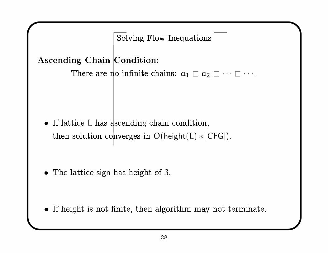
Solving Flow InequationsAs ending Chain Condition:There are no in�nite hains: a1 ⊏ a2 ⊏ · · · ⊏ · · · .
� If latti e L has as ending hain ondition,then solution onverges in O(height(L) ∗ |CFG|).
� The latti e sign has height of 3.
� If height is not �nite, then algorithm may not terminate.
28

Interval Analysis29

Intervals: Basi Fa tsInterval: z ∈ [a, b]∆= {z|a ≤ z ≤ b}
We will onsider intervals of integer values.
Half-open Intervals: z ∈ [a, ∞) and z ∈ (−∞, a].
Interval Latti e: [a, b] ⊑ [c, d] i� a ≥ c ∧ b ≤ d.
Con retization: [[[a, b]]] = {z|a ≤ z ≤ b}
Abstra tion: Given I ⊆ Z, α(I) = [min≤(I), max≤(I)].
30

Interval Latti e
⊤
... ... ... ... ... ... ...
[0, 0] [1, 1] [2, 2] [3, 3] [4, 4] [5, 5] [6, 6] [7, 7] · · ·
⊥
Note: Latti e is omplete.However, it has in�nite height (and width).
31

Interval Analysis: Example # 2
n0 : x := 0 (−∞, ∞) ⊑ Rng(n0, x)
n1 : + post(x := 0, Rng(n0, x)) ⊑ Rng(n1, x)
n2 : x < 100 Rng(n1, x) ⊑ Rng(n2, x)
n3 : x := x + 2 Rng(n2, x) ⊓ α([[x < 100]]) ⊑ Rng(n3, x)
post(x := x + 2, Rng(n3, x)) ⊑ Rng(n1, x)
32

Interval Analysis: Solving Data�ow Equations
Notation: Ri : Rng(ni, x).(−∞, ∞) ⊑ R0 ⊥ ⊤ ⊤ ⊤ ⊤
post(n0, R0) ⊔ post(n3, R3) ⊑ R1 ⊥ [0, 0] [0, 0] [0, 0] [0, 1]
R1 ⊑ R2 ⊥ ⊥ [0, 0] [0, 0] [0, 0]
R2 ⊓ [0, 99] ⊑ R3 ⊥ ⊥ ⊥ [0, 0] [0, 0]This pro ess onverges in 100x steps to the following solution:
R0 : ⊤, R1 : [0, 100], R2 : [0, 100], R3 : [0, 99] .
33

Interval Analysis: Example #3
n0 : x := 0 (−∞, ∞) ⊑ Rng(n0, x)
[0, ∞) ⊑ Rng(n0, n)
n1 : + post(x := 0, Rng(n0, x)) ⊑ Rng(n1, x)
n2 : x < n Rng(n1, x) ⊑ Rng(n2, x)
n3 : x := x + 2 Rng(n2, x) ⊓ α([[x < n]]) ⊑ Rng(n3, x)
post(x := x + 2, Rng(n3, x)) ⊑ Rng(n1, x)
34

Solving Data�ow Equations
Notation: Ri : Rng(ni, x).(−∞, ∞) ⊑ R0 ⊥ ⊤ ⊤ ⊤ ⊤
post(n0, R0) ⊔ post(n3, R3) ⊑ R1 ⊥ [0, 0] [0, 0] [0, 0] [0, 1]
R1 ⊑ R2 ⊥ ⊥ [0, 0] [0, 0] [0, 0]
R2 ⊓ [0, ∞) ⊑ R3 ⊥ ⊥ ⊥ [0, 0] [0, 0]This pro ess does not onverge in �nitely many steps.The least �xed point solution is:R0 : ⊤, R1 : [0, ∞), R2 : [0, ∞), R3 : [0, ∞) .Question: How do we ompute �xed points in the interval latti e?
35

Widening� The Interval latti e has in�nite height.� Widening operator: Let [a, b] ⊑ [c, d].
[a, b]∇[c, d] = [ℓ, u]wherein
ℓ =
−∞ if c < a,
c otherwiseand similarly,
u =
∞ if d > b,
b otherwise� Spe ial ase: ⊥∇i = i. 36

Widening: Examples
Examples:[−1, −1] ∇ [−5, −5] = (−∞, +∞)
[1, 1] ∇ [1, 2] = [1, +∞)
[1, 1] ∇ [−1, 1] = (−∞, 1]
[−1, 5] ∇ [−1, 5] = (−1, 5)
⊥ ∇ [10, 100] = [10, 100]
37

Widening: PropertiesProperties: The following properties are true of widening.
(A) (∀x ⊑ y) x ⊔ y ⊑ x∇yLet a1 ⊏ a2 ⊏ a3 ⊏ · · · be an in reasing sequen e.
Widened sequen e: b1 = a1, bi+1 = bi∇(bi ⊔ ai).
Theorem: Widened sequen e onverges in �nitely many steps, i.e.,
b1 ⊑ b2 ⊑ b3 · · · ⊑ bN = bN+1 = bN+2 · · · .and
max⊑{a1, . . . , } ⊑ bN .
38

Widening: Appli ationConsider Data�ow Inequalities:
f1(x1, . . . , xn) ⊑ x1...
fn(x1, . . . , xn) ⊑ xnInitial step: ⟨
x01, . . . , x0
n
⟩
= 〈⊥, . . . ,⊥〉.Widening Iteration: We split iteration into two steps:Step 1: ⟨
yi1, . . . , yi
n
⟩
=⟨
f1(xi1, . . . , xi
n), . . . , fn(xi1, . . . , xi
n)⟩.Step 2: ⟨
xi+11 , . . . , xi+1
n
⟩
=⟨
xi1, . . . , xi
n
⟩
∇⟨
yi1, . . . , yi
n
⟩.
Convergen e: (∀j ∈ [1, n]) yNj ⊑ xN
j .39

Widening: Example
Carry out the widening iteration for Example# 3.
40

Widening Iteration� Widening iteration produ es a solution to the data�owinequalities.(∀j ∈ [1, n]) fj(x
N1 , . . . , xN
n ) ⊑ xj . (1)� However, there are two problems:(a) Solution is no longer the least �xed point. Su h solutionsare alled post-�xed points.(b) Solution improvement may be possible. By monotoni ity,
f(x) ⊑ x ⇒ f(f(x)) ⊑ f(x) .Therefore, if x is a post-�xed point solution then f(x) maybe a smaller post-�xed point.41

As ending/Des ending Iterations
f(xN) ⊑ xN Widening post-�xed point
f(xN)
f2(xN) Des ending iteration
xi+1 = xi∇f(xi) fi(xN) = fi+1(xN)
f∗(⊥) Least �xed point
x2 = x1∇f(x1)
x1 = f(⊥)∇f2(⊥) f3(⊥)
f2(⊥)
f(⊥)
⊥
42

Des ending Iteration: Example #2
Carry out the widening iteration and des ending iteration forExample# 2.
43

Des ending Iteration: Convergen eDes ending Chain Condition: Dual to As ending Chain ondition.Des ending iteration need not ne essarily onverge in �nitely manysteps.
(1) Stop the iteration after some �xed number of steps.This is not a good idea (provide an example).
(2) Use a �narrowing� operator to for e onvergen e.
44