Topic 22

Analysis of Variance

22.1 OverviewTwo-sample t procedures are designed to compare the means of two populations. Our next step is to compare themeans of several populations. We shall explain the methodology through an example. Consider the data set gatheredfrom the forests in Borneo.

Example 22.1 (Rain forest logging). The data on 30 forest plots in Borneo are the number of trees per plot.

never logged logged 1 year ago logged 8 years agoni 12 12 9yi 23.750 14.083 15.778si 5.065 4.981 5.761

We compute these statistics from the data y11

, . . . y1n1 , y

21

, . . . y2n2 and y

31

, . . . y2n2

yi =1

ni

ni

X

j=1

yij and s2i =

1

ni � 1

ni

X

j=1

(yij � yi)2

One way analysis of variance (ANOVA) is a statistical procedure that allows us to test for the differences inmeans for two or more independent groups. In the situation above, we have set our design so that the data in each ofthe three groups is a random sample from within the groups. The basic question is: Are these means the same (the nullhypothesis) or not (the alternative hypothesis)?

never logged logged 1 year ago logged 8 years ago

510

15

20

25

30

35

Figure 22.1: Side-by-side boxplots of the number of trees per plot.The groups will be considered different if the differences between thegroups (indicated by the variation in the center lines of the boxes) islarge compared to the width of the boxes in the boxplot.

As the case with the t procedures, the appropriatenessof one way analysis of variance is based on the applica-bility of the central limit theorem. As with t procedures,ANOVA has an alternative, the Kruskal-Wallis test, basedon the ranks of the data for circumstances in which the cen-tral limit theorem does not apply.

The basic idea of the test is to examine the ratio ofs2between

, the variance between the groups 1, 2, and 3. ands2residual

, a statistic that measures the variances within thegroups. If the resulting ratio test statistic is sufficientlylarge, then we say, based on the data, that the means ofthese groups are distinct and we are able to reject the nullhypothesis. Even though the boxplots use different mea-sures of center (median vs. mean) and spread (quartiles vs.standard deviation), this idea can be expressed by examin-ing the fluctuation in the centers of boxes in Figure 22.1 compared to the width of the boxes.

339

Introduction to the Science of Statistics Analysis of Variance

As we have seen before, this decision to reject H0

will be the consequence a sufficiently high value of a test statistic- in this case the F statistic. The distribution of this test statistic will depend on the number of groups (3 in the exampleabove) and the number of total observations (33 in the example above). Consequently, variances between groups thatare not that are not statistically significant for small sample sizes can become significant as the sample sizes and, withit, the power increase.

22.2 One Way Analysis of VarianceFor one way analysis of variance, we expand to more than the two groups seen for t procedures and ask whether ornot the means of all the groups are the same. The hypothesis in this case is

H0

: µj = µk for all j, k and H1

: µj 6= µk for some j, k.

The data {yij , 1 i nj , 1 j q} represents that we have ni observation for the i-th group and that we haveq groups. The total number of observations is denoted by n = n

1

+ · · ·+ nq . The model is

yij = µi + ✏ij .

where ✏ij are independent N(0,�) random variables with �2 unknown. This allows us to define the likelihood andto use that to determine the analysis of variance F test as a likelihood ratio test. Notice that the model for analysisrequires a common value � for all of the observations.

In order to develop the F statistic at the test statistic, we will need to introduce two types of sample means:

• The within group means is simply the sample mean of the observations inside each of the groups,

yj =1

nj

nj

X

i=1

yij , j = 1. . . . , q.

These are given in the table in Example 22.1 for the Borneo rains forest.

• The mean of the data taken as a whole, known as the grand mean,

y =

1

n

qX

j=1

nj

X

i=1

yij =1

n

qX

j=1

nj yj .

This is the weighted average of the yi with weights ni, the sample size in each group. The Borneo rain forestexample has an overall mean

y =

1

n

3

X

j=1

nj yj =1

12 + 12 + 9

(12 · 23.750 + 12 · 14.083 + 9 · 15.778) = 18.06055.

Analysis of variance uses the total sums of squares

SStotal

=

qX

j=1

nj

X

i=1

(yij � y)2, (22.1)

the total square variation of individual observations from their grand mean. However, the test statistic is determinedby decomposing SS

total

. We start with a bit of algebra to rewrite the interior sum in (22.1) asnj

X

i=1

(yij � y)2 =

nj

X

i=1

(yij � yj)2

+ nj(yj � y)2 = (nj � 1)s2j + nj(yj � y)2. (22.2)

Here, s2j is the unbiased estimator of the variance based on the observations in the j-th group.

340

Introduction to the Science of Statistics Analysis of Variance

source of degrees of sums of meanvariation freedom squares squarebetween groups q � 1 SS

between

s2between

= SSbetween

/(q � 1)

residuals n� q SSresidual

s2residual

= SSresidual

/(n� q)

total n� 1 SStotal

Table I: Table for one way analysis of variance

Exercise 22.2. Show the first equality in (22.2). (Hint: Begin with the difference in the two sums.)

Together (22.1) and (22.2) yields the decomposition of the variation

SStotal

= SSresidual

+ SSbetween

with

SSresidual

=

qX

j=1

nj

X

i=1

(yij � yj)2

=

qX

j=1

(nj � 1)s2j and SS2

between

=

qX

j=1

nj(yj � y)2.

For the rain forest example, we find that

SSbetween

=

3

X

j=1

nj(yj � y)2 = 12 · (23.750� y)2 + 12 · (14.083� y)2 + 9 · (15.778� y)2) = 625.1793

and

SSresidual

=

3

X

j=1

(nj � 1)s2j = (12� 1) · 5.0652 + (12� 1) · 4.9812 + (9� 1) · 5.7612 = 820.6234

From this, we obtain the general form for one-way analysis of variance as shown in Table I.

• The q � 1 degrees of freedom between groups is derived from the q groups minus one degree of freedom usedto compute y.

• The n� q degrees of freedom within the groups is derived from the nj � 1 degree of freedom used to computethe variances s2j . Add these q values for the degrees of freedom to obtain n� q.

The test statistic

F =

s2between

s2residual

=

SSbetween

/(q � 1)

SSresidual

/(n� q).

source of degrees of sums of meanvariation freedom squares squarebetween groups 2 625.2 312.6residuals 30 820.6 27.4total 32 1445.8

Table II: Analysis of variance information for the Borneo rain forest data

341

Introduction to the Science of Statistics Analysis of Variance

is, under the null hypothesis, a constant multiple of the ratio of two independent �2 random variables with parameterq�1 for the numerator and n�q for the denominator. This ratio is called an F random variable with q�1 numeratordegrees of freedom and n� q denominator degrees of freedom.

Using Table II, we find the value of the test statistic for the rain forest data is

F =

s2between

s2residual

=

312.6

27.4= 11.43.

and the p-value (calculated below) is 0.0002. The critical value for an ↵ = 0.01 level test is 5.390. So, we do rejectthe null hypothesis that mean number of trees does not depend on the history of logging.

> 1-pf(11.43,2,30)[1] 0.0002041322> qf(0.99,2,30)[1] 5.390346

0 1 2 3 4 5 6 7

0.0

0.2

0.4

0.6

0.8

1.0

x

df(

x, 2, 30)

0 1 2 3 4 5 6 7

0.0

0.2

0.4

0.6

0.8

1.0

0 1 2 3 4 5 6 7

0.0

0.2

0.4

0.6

0.8

1.0

0 1 2 3 4 5 6 7

0.0

0.2

0.4

0.6

0.8

1.0

0 1 2 3 4 5 6 7

0.0

0.2

0.4

0.6

0.8

1.0

0 1 2 3 4 5 6 7

0.0

0.2

0.4

0.6

0.8

1.0

Figure 22.2: Upper tail critical values. The density for an F random variablewith numerator degrees of freedom, 2, and denominator degrees of freedom, 30.The indicated values 3.316, 4.470, and 5.390 are critical values for significancelevels ↵ = 0.05, 0.02, and 0.01, respectively.

Confidence intervals are determined using thedata from all of the groups as an unbiased estimatefor the variance, �2. Using all of the data allowsus to increase the number of degrees of freedom inthe t distribution and thus reduce the upper criticalvalue for the t statistics and with it the margin oferror.

The variance s2residuals

is given by the expres-sion SS

residuals

/(n � q), shown in the table inthe “mean square” column and the “residuals” row.The standard deviation s

residual

is the square rootof this number. For example, the �-level confi-dence interval for µj is

yj ± t(1��)/2,n�q

sresidualp

nj.

The confidence for the difference in µj�µk is sim-ilar to that for a pooled two-sample t confidenceinterval and is given by

yj � yk ± t(1��)/2,n�qsresidual

s

1

nj+

1

nk.

In this case, the 95% confidence interval for the mean number of trees on a lot“logged 1 year ago” has n � q =

33� 3, t0.025,30 = 2.042, s

residual

=

p27.4 = 5.234 and the confidence interval is

14.083± 2.042

p27.4p12

= 14.083± 4.714 = (9.369, 18.979).

Exercise 22.3. Give the 95% confidence intervals for the difference in trees between plots never logged and plotslogged 8 years ago.

Example 22.4. The development time for a European queen in a honey bee hive is suspected to depend on the tem-perature of the hive. To examine this, queens are reared in a low temperature hive (31.1� C), a medium temperaturehive (32.8� C) and a high temperature hive (34.4� C). The hypothesis is that higher temperatures increase metabolismrate and thus reduce the time needed from the time the egg is laid until an adult queen honey bee emerges from thecell. The hypothesis is

H0

: µlow

= µmed

= µhigh

versus H1

: µlow

, µmed

, µhigh

differ

342

Introduction to the Science of Statistics Analysis of Variance

1 2 3

14.0

14.5

15.0

15.5

16.0

16.5

Figure 22.3: Side-by-side boxplot of queen development times. The time is measured in days. the plots show cool (1) medium (2) and warm (3)hive temperatures.

where µlow

, µmed

, and µhigh

are, respectively, the mean development time in days for queen eggs reared in a low, amedium, and a high temperature hive.

Here are the data and a boxplot:

> ehblow<-c(16.2,14.6,15.8,15.8,15.8,15.8,16.2,16.7,15.8,16.7,15.3,14.6,15.3,15.8)

> ehbmed<-c(14.5,14.7,15.9,15.5,14.7,14.7,14.7,15.5,14.7,15.2,15.2,15.9,14.7,14.7)

> ehbhigh<-c(13.9,15.1,14.8,15.1,14.5,14.5,14.5,14.5,13.9,14.5,14.8,14.8,13.9,14.8,14.5,14.5,14.8,14.5,14.8)

> boxplot(ehblow,ehbmed,ehbhigh)

The commands in R to perform analysis and the output are shown below. The first line put all of the data in asingle vector, ehb. We then put labels for the groups in the variable or factor temp. Expressed in this way, thisvariable is considered by R as a numerical vector. To tell R that it should be thought of as a factor and list the factorsin the vector ftemp. Without this, the command anova(lm(ehb⇠temp)) would attempt to do linear regressionwith temp as the explanatory variable.

> ehb<-c(ehblow,ehbmed,ehbhigh)> temp<-c(rep(1,length(ehblow)),rep(2,length(ehbmed)),rep(3,length(ehbhigh)))> ftemp<-factor(temp,c(1:3))> anova(lm(ehb˜ftemp))Analysis of Variance Table

Response: ehbDf Sum Sq Mean Sq F value Pr(>F)

ftemp 2 11.222 5.6111 23.307 1.252e-07 ***Residuals 44 10.593 0.2407---Signif. codes: 0 *** 0.001 ** 0.01 * 0.05 . 0.1 1

343

Introduction to the Science of Statistics Analysis of Variance

The anova output shows strong evidence against the null hypothesis. The p-value is 1.252 ⇥ 10

�7. The values inthe table can be computed directly from the formulas above.

For the sums of square between groups, SSbetween

,

> length(ehblow)*(mean(ehblow)-mean(ehb))ˆ2+ length(ehbmed)*(mean(ehbmed)-mean(ehb))ˆ2+ length(ehbhigh)*(mean(ehbhigh)-mean(ehb))ˆ2

[1] 11.22211

and within groups, SSresidual

,

> sum((ehblow-mean(ehblow))ˆ2)+sum((ehbmed-mean(ehbmed))ˆ2)+ sum((ehbhigh-mean(ehbhigh))ˆ2)

[1] 10.59278

For confidence intervals we use s2resid = 0.2407, sresid = 0.4906 and the t-distribution with 44 degrees offreedom.

For the medium temperature hive, the 95% confidence interval for µmed can be computed

> mean(ehblow)[1] 15.74286> qt(0.975,44)[1] 2.015368> length(ehblow)[1] 14

Thus, the intverval is

ymed ± t0.025,44

sresidpnmed

= 15.742± 2.01540.4906p

14

= (15.478, 16.006)

22.3 ContrastsAfter completing a one way analysis of variance, resulting in rejecting the null hypotheses, a typical follow-up proce-dure is the use of contrasts. Contrasts use as a null hypothesis that some linear combination of the means equals tozero.

Example 22.5. If we want to see if the rain forest has seen recovery in logged areas over the past 8 years. This canbe written as

H0

: µ2

= µ3

versus H1

: µ2

6= µ3

.

orH

0

: µ2

� µ3

= 0 versus H1

: µ2

� µ3

6= 0

Under the null hypothesis, the test statistic

t =y2

� y3

sresidualq

1

n2+

1

n3

,

has a t-distribution with n� q degrees of freedom. Here

t =14.083� 15.778

5.234q

1

12

+

1

9

= �0.7344,

with n� q = 33� 3 degrees of freedom, the p-value for this 2-sided test is

344

Introduction to the Science of Statistics Analysis of Variance

> 2*pt(-0.7344094,30)[1] 0.4684011

is considerably too high to reject the null hypothesis.

Example 22.6. To see if the mean queen development medium hive temperature is midway between the time for thehigh and low temperature hives, we have the contrast,

H0

:

1

2

(µlow + µhigh) = µmed versus H1

:

1

2

(µlow + µhigh) 6= µmed

orH

0

:

1

2

µlow � µmed +1

2

µhigh = 0 versus H1

:

1

2

µlow � µmed +1

2

µhigh 6= 0

Notice that, under the null hypothesis

E

1

2

¯Ylow � ¯Ymed +1

2

¯Yhigh

�

=

1

2

µlow � µmed +1

2

µhigh = 0

and

Var✓

1

2

¯Ylow � ¯Ymed +1

2

¯Yhigh

◆

=

1

4

�2

nlow+

�2

nmed+

1

4

�2

nhigh.

This leads to the test statistic

t =1

2

ylow � ymed +1

2

yhigh

sresidualq

1

4nlow

+

1

nmed

+

1

4nhigh

=

1

2

15.743� 15.043 + 1

2

14.563

0.4906q

1

4·14 +

1

14

+

1

4·19

= 0.7005.

The p-value,

> 2*(1-pt(0.7005,44))[1] 0.487303

again, is considerably too high to reject the null hypothesis.

Exercise 22.7. Under the null hypothesis appropriate for one way analysis of variance, with ni observations in groupi = 1, . . . , q and ¯Yi =

Pni

j=1

Yij/ni,

E[c1

¯Y1

+ · · ·+ Yqµq] = c1

µ1

+ · · ·+ cqµq, Var(c1

¯Y1

+ · · ·+ cqYq) =c21

�2

n1

+ · · ·+c2q�

2

nq.

In general, a contrast begins with a linear combination of the means

= c1

µ1

+ · · ·+ cqµq.

The hypothesis isH

0

: = 0 versus H1

: 6= 0

For sample means, y1

, . . . , yq , the test statistic is

t =c1

y1

+ · · ·+ cq yq

sresidual

q

c21n1

+ · · ·+ c2q

nq

.

Under the null hypothesis the t statistic has a t distribution with n� q degrees of freedom.

345

Introduction to the Science of Statistics Analysis of Variance

22.4 Two Sample ProceduresWe now show that the t-sample procedure results from a likelihood ratio test. We keep to two groups in the devel-opment of the F test. The essential features can be found in this example without the extra notation necessary for anarbitrary number of groups.

Our hypothesis test is based on two independent samples of normal random variables. The data are

yij = µj + ✏ij .

where ✏ij are independent N(0,�) random variables with � unknown. Thus, we have nj independent N(µj ,�)random variables Y

1j . . . , Ynj

j with unknown common variance �2, j = 1 and 2. The assumption of a commonvariance is critical to the ability to compute the test statistics.

Consider the two-sided hypothesis

H0

: µ1

= µ2

versus H1

: µ1

6= µ2

.

Thus, the parameter space is⇥ = {(µ

1

, µ2

,�2

);µ1

, µ2

2 R,�2 > 0}.

For the null hypothesis, the possible parameter values are

⇥

0

= {(µ1

, µ2

,�2

);µ1

= µ2

,�2 > 0}

Step 1. Determine the log-likelihood. To find the test statistic derived from a likelihood ratio test, we first writethe likelihood and its logarithm based on observations y = (y

11

, . . . , yn11, y12, . . . , yn22).

L(µ1

.µ2

,�2|y) =✓

1p2⇡�2

◆n1+n2

exp� 1

2�2

n1X

i=1

(yi1 � µ1

)

2

+

n2X

i=1

(yi2 � µ2

)

2

!

(22.3)

lnL(µ1

.µ2

,�2|y) = � (n1

+ n2

)

2

(ln 2⇡ + ln�2

)� 1

2�2

n1X

i=1

(yi1 � µ1

)

2

+

n2X

i=1

(yi2 � µ2

)

2

!

(22.4)

Step 2. Find the maximum likelihood estimates and the maximum value of the likelihood. By taking partialderivatives with respect to µ

1

and µ2

we see that with two independent samples, the maximum likelihood estimate forthe mean µj for each of the samples is the sample mean yj .

µ1

= y1

=

1

n1

n1X

i=1

yi1, µ2

= y2

=

1

n2

n2X

i=1

yi2.

Now differentiate (22.4) with respect to �2

@

@�2

lnL(µ1

, µ2

,�2|x) = �n1

+ n2

2�2

+

1

2(�2

)

2

n1X

i=1

(yi1 � µ1

)

2

+

n2X

i=1

(yi2 � µ2

)

2

!

.

Thus, the maximum likelihood estimate of the variance is the weighted average, weighted according to the samplesize, of the maximum likelihood estimator of the variance for each of the respective samples.

�2

=

1

n1

+ n2

n1X

i=1

(yi1 � y1

)

2

+

n2X

i=1

(yi2 � y2

)

2

!

.

346

Introduction to the Science of Statistics Analysis of Variance

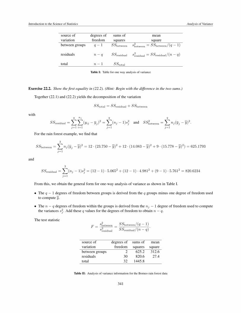
Now, substitute these values into the likelihood (22.3) to see that the maximum value for the likelihood is

L(µ1

, µ2

, �2|x) = 1

(2⇡�2

)

(n1+n2)/2exp� 1

2�2

n1X

i=1

(yi1 � y1

)

2

+

n2X

i=1

(yi2 � y2

)

2

!

=

1

(2⇡�2

)

(n1+n2)/2exp�n

1

+ n2

2

Step 3. Find the parameters that maximize the likelihood under the null hypothesis and then find themaximum value of the likelihood on ⇥

0

. Next, for the likelihood ratio test, we find the maximum likelihood underthe null hypothesis. In this case the two means have a common value which we shall denote by µ.

L(µ,�2|y) =✓

1p2⇡�2

◆n1+n2

exp� 1

2�2

n1X

i=1

(yi1 � µ)2 +n2X

i=1

(yi2 � µ)2!

(22.5)

lnL(µ,�2|x) = � (n1

+ n2

)

2

(ln 2⇡ + ln�2

)� 1

2�2

n1X

i=1

(yi1 � µ)2 +n2X

i=1

(yi2 � µ)2!

(22.6)

The µ derivative of (22.6) is

@

@µlnL(µ,�2|x) = 1

�2

n1X

i=1

(yi1 � µ) +n2X

i=1

(yi2 � µ)

!

.

Set this to 0 and solve to realize that the maximum likelihood estimator under the null hypothesis is the grand samplemean y obtained by considering all of the data being derived from one large sample

µ0

= y =

1

n1

+ n2

n1X

i=1

yi1 +n2X

i=1

yi2

!

=

n1

y1

+ n2

y2

n1

+ n2

.

Intuitively, if the null hypothesis is true, then all of our observations are independent and have the same distributionand thus, we should use all of the data to estimate the common mean of this distribution.

The value for �2 that maximizes (22.5) on ⇥

0

, is also the maximum likelihood estimator for the variance obtainedby considering all of the data being derived from one large sample:

�2

0

=

1

n1

+ n2

n1X

i=1

(yi1 � y)2 +n2X

i=1

(yi2 � y)2!

.

We can find that the maximum value on ⇥

0

for the likelihood is

L(µ0

, �2

0

|x) = 1

(2⇡�2

0

)

(n1+n2)/2exp� 1

2�2

0

n1X

i=1

(yi1 � y)2 +n2X

i=1

(yi2 � y)2!

=

1

(2⇡�2

0

)

(n1+n2)/2exp�n

1

+ n2

2

Step 4. Find the likelihood statistic ⇤(y). From steps 2 and 3, we find a likelihood ratio of

⇤(y) =L(µ

0

, �2

0

|x)L(µ, �2|x) =

✓

�2

0

�2

◆�(n1+n2)/2

=

✓

Pn1

i=1

(yi1 � y)2 +Pn2

i=1

(yi2 � y)2Pn1

i=1

(yi1 � y1

)

2

+

Pn2

i=1

(yi2 � y2

)

2

◆�(n1+n2)/2

. (22.7)

This is the ratio, SStotal, of the variation of individuals observations from the grand mean and SSresiduals. thevariation of these observations from the mean of its own groups.

347

Introduction to the Science of Statistics Analysis of Variance

Step 5. Simplify the likelihood statistic to determine the test statistic F . Traditionally, the likelihood ratio issimplified by looking at the differences of these two types of variation, the numerator in (22.7)

SStotal

=

n1X

i=1

(yi1 � y)2 +n2X

i=1

(yi2 � y)2

and the denominator in (22.7)

SSresiduals

=

n1X

i=1

(yi1 � y1

)

2

+

n2X

i=1

(yi2 � y2

)

2

Exercise 22.8. Show that SStotal

� SSresiduals

= n1

(y1

� y)2 + n2

(y2

� y)2.

In words, SStotal

the sums of squares of the differences of an individual observation from the overall mean y, isthe sum of two sources. The first is the sums of squares of the difference of the average of each group mean and theoverall mean,

SSbetween

= n1

(y � y1

)

2

+ n2

(y � y2

)

2.

The second is the sums of squares of the difference of the individual observations with its own group mean, SSresiduals

.Thus, we can write

SStotal

= SSresidual

+ SSbetween

Now, the likelihood ratio (22.7) reads

⇤(y) =

✓

SSresidual

+ SSbetween

SSresiduals

◆

=

✓

1 +

SSbetween

SSresiduals

◆�(n1+n2)/2

Due to the negative power in the exponent, the critical region ⇤(y) �0

is equivalent to

SSbetween

SSresiduals

=

n1

(y � y1

)

2

+ n2

(y � y2

)

2

(n1

� 1)s21

+ (n2

� 1)s22

� c (22.8)

for an appropriate value c. The ratio in (22.8) is, under the null hypothesis, a multiple of an F -distribution. The laststep to divide both the numerator and denominator by the degrees of freedom. Thus, we see, as promised, we reject ifthe F -statistics is too large, i.e., the variation between the groups is sufficiently large compared to the variation withinthe groups.

Exercise 22.9 (pooled two-sample t-test). For an ↵ level test, show that the test above is equivalent to

|T (y)| > t↵/2,n1+n+2

.

whereT (y) =

y1

� y2

spq

1

n1+

1

n2

.

and sp is the standard deviation of the data pooled into one sample.

s2p =

1

n1

+ n2

� 2

�

(n1

� 1)s21

+ (n2

� 1)s22

�

Exercise 22.10. Generalize the formulae for y, SSbetween

and SSresiduals

from the case q = 2 to an arbitrary numberof groups.

348

Introduction to the Science of Statistics Analysis of Variance

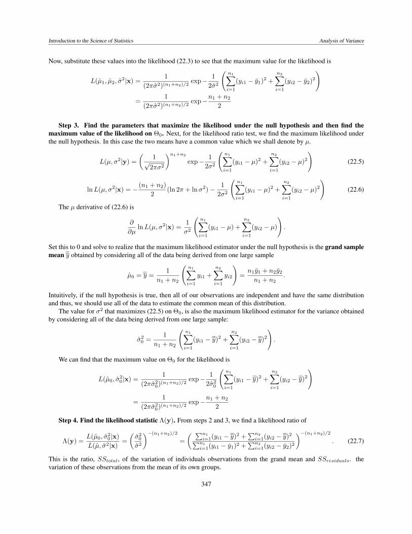
Thus, we can use the two-sample procedure to compare any two of the three groups. For example, to comparedthe never logged forest plots to those logged 8 years ago., we find the pooled variance

s2p =

1

n1

+ n2

� 2

((n1

� 1)s21

+ (n2

� 1)s22

) =

1

19

(11 · 5.0652 + 8 · 5.7612) = 28.827

and sp = 5.37. Thus, the t-statistic

t =23.750� 15.778

5.37q

1

12

+

1

9

= 7.644.

> 1-pt(7.644,19)[1] 1.636569e-07

Thus, the p-value at 1.64⇥ 10

7 is strong evidence against the null hypothesis.

22.5 Kruskal-Wallis Rank-Sum TestThe Kruskal-Wallis test is an alternative to one-way analysis of variance in much the same way that the Wilcoxonrank-sum test is a alternative to two-sample t procedures. Like the Wilcoxon test, we replace the actual data with theirranks. This non-parametric alternative obviates the need to use the normal distribution arising from an application ofthe central limit theorem. The H test statistic has several analogies with the F statistic. To compute this statistic:

• Replace the data {yij , 1 i nj , 1 j q} for ni observations for the i-th group from each of the q groupswith {rij , 1 i nj , 1 j q}, the ranks of the data taking all of the groups together. For ties, average theranks.

• The total number of observations n = n1

+ · · ·+ nq .

• The average rank within the groups

ri =1

ni

ni

X

j=1

rij , i = 1, . . . , q.

• The grand average of the ranks

r =

1

n(1 + · · ·+ n) =

1

nn(n+ 1) =

n+ 1

2

.

(See Exercise 20.6.)

• The Kruskal-Wallis test statistic looks at the sums of squares of ranks between groups and the total sum ofsquares of ranks

H =

SSRbetween

SSRtotal

/(n� 1)

=

Pgi=1

ni(ri � r)2Pq

i=1

Pni

j=1

(rij � r)2/(n� 1)

,

• For larger data sets (each ni � 5), the p-value is approximately the probability that a �2

q�1

random variableexceeds the value of the H statistic.

• For smaller data sets, more sophisticated procedures are necessary.

• The test can be followed by using a procedure analogous to contrasts based on the Wilcoxon rank-sum test.

Exercise 22.11. For the case of no ties, show that

SSRtotal

=

(n� 1)n(n+ 1)

12

349

Introduction to the Science of Statistics Analysis of Variance

In this case,

H =

12

n(n+ 1)

qX

i=1

ni

✓

ri �n+ 1

2

◆

2

=

12

n(n+ 1)

qX

i=1

nir2

i � 3(n+ 1).

The Kruskal-Wallis test also gives a very small p-value to the queen development times for Africanized honeybees. Begin with the R commands in Example 22.4 to enter the data and create the temperature factors ftemp.

> kruskal.test(ehb˜ftemp)

Kruskal-Wallis rank sum test

data: ehb by ftempKruskal-Wallis chi-squared = 20.4946, df = 2, p-value = 3.545e-05

22.6 Answer to Selected Exercises22.2. Let’s look at this difference for each of the groups.

ni

X

j=1

(yij � y)2 �ni

X

j=1

(yij � yi)2

=

ni

X

j=1

�

(yij � y)2 � (yij � yi)2

�

=

ni

X

j=1

(2yij � y � yi)(�y + yi) = ni(2yi � y � yi)(�y + yi) = ni(yi � y)2

Now the numerator in (22.7) can be written to show the decomposition of the variation into two sources - the withingroup variation and the between group variation.

n1X

i=1

(yi1 � y)2 +n2X

i=1

(yi2 � y)2 =

n1X

i=1

(y1j � y

1

)

2

+

n2X

i=1

(y2j � y

2

)

2

+ n1

(y � y1

)

2

+ n2

(y � y2

)

2.

= (n1

� 1)s21

+ (n2

� 1)s22

+ n1

(y � y1

)

2

+ n2

(y � y2

)

2.

22.3. Here, we are looking for a confidence interval for µ1

� µ3

. From the summaries, we need

n1

= 12, y1

= 23.750, n3

= 9, y3

= 17.778.

From the computation for the test, we have sresidual

=

p27.4 = 5.234 and using the qt(0.975,30) command we

find t0.025,30 = 2.042. Thus,

(y1

� y3

) ±t(0.975,30)sresidual

r

1

n1

+

1

n3

= (23.750� 17.778) ±2.042 · 5.234r

1

12

+

1

9

= 5.972 ±2.079 = (3.893, 8.051)

22.7. This follows from the fact that expectation is a linear functional and the generalized Pythagorean identity for thevariance of a linear combination of independent random variables.

350

Introduction to the Science of Statistics Analysis of Variance

22.8. Look at the solution to Exercise 22.2.

22.9. We will multiply the numerator in (22.8) by (n1

+ n2

)

2 and note that (n1

+ n2

)y = n1

y1

+ n2

y2

. Then,

(n1

+ n2

)

2

(n1

(y � y1

)

2

+ n2

(y � y2

)

2

= n1

((n1

+ n2

)y � (n1

+ n2

)y1

)

2

+ n2

((n1

+ n2

)y � (n1

+ n2

)y2

)

2

= n1

(n1

y1

+ n2

y2

� (n1

+ n2

)y1

)

2

+ n2

(n1

y1

+ n2

y2

� (n1

+ n2

)y2

)

2

= n1

(n2

(y2

� y1

))

2

+ n2

(n1

(y1

� y2

))

2

= (n1

n2

2

+ n2

n2

1

)(y1

� y2

)

2

= n1

n2

(n1

+ n2

)(y1

� y2

)

2

Consequently

(n1

(y � y1

)

2

+ n2

(y � y2

)

2

=

n1

n2

n1

+ n2

(y1

� y2

)

2

= (y1

� y2

)

2/

✓

1

n1

+

1

n2

◆

.

The denominatorn1X

j=1

(yi1 � y1

)

2

+

n2X

j=1

(yi2 � y2

)

2

= (n1

+ n2

� 2)s2p.

The ratioSS

between

SSresiduals

=

(y1

� y2

)

2

(n1

+ n2

� 2)s2p

⇣

1

n1+

1

n2

⌘

=

T (y)2

n1

+ n2

� 2

.

Thus, the test is a constant multiple of the square of the t-statistic. Take the square root of both sides to create a testusing a threshold value for |T (y)| for the critical region.

22.10. For observations, yi1, . . . yini

in group i = 1, . . . , q, let n = n1

+ · · ·+nq be the total number of observations,then the grand mean

y =

1

n(n

1

y1

+ · · ·+ nq yq)

where yi is the sample mean of the observations in group i. The sums of squares are

SSbetween

=

qX

i=1

ni(yi � y)2 and SSresiduals

=

qX

i=1

(ni � 1)s2i

where s2i is the sample variance of the observations in group i.

22.11. In anticipation of its need, let’s begin by showing thatnX

j=1

j2 =

n(n+ 1)(2n+ 1)

6

.

Notice that the formula holds for the case n = 1 with

1

2

=

1(1 + 1)(2 · 1 + 1)

6

=

6

6

= 1.

Now assume that the identity holds for n = k. We then check that it also holds for n = k + 1

1

2

+ 2

2

+ · · ·+ k2 + (k + 1)

2

=

k(k + 1)(2k + 1)

6

+ (k + 1)

2

=

k + 1

6

(k(2k + 1) + 6(k + 1)) =

k + 1

6

(2k2 + 7k + 6)

=

(k + 1)(k + 2)(2k + 3)

6

351

Introduction to the Science of Statistics Analysis of Variance

This is the formula for n = k + 1 and so by the mathematical induction, we have the identity for all non-negativeintegers.

With no ties, each rank appears once and

SSRtotal

=

nX

j=1

✓

j � n+ 1

2

◆

2

=

nX

j=1

j2 � 2

nX

j=1

jn+ 1

2

+

nX

j=1

✓

n+ 1

2

◆

2

=

n(n+ 1)(2n+ 1)

6

� 2

n(n+ 1)

2

n+ 1

2

+ n

✓

n+ 1

2

◆

2

=

n(n+ 1)(2n+ 1)

6

� n(n+ 1)

2

4

=

n(n+ 1)

12

(2(2n+ 1)� 3(n+ 1)) =

(n� 1)n(n+ 1)

12

.

352