One-Way Analysis of Variance

(ANOVA):

Between-Participants Design

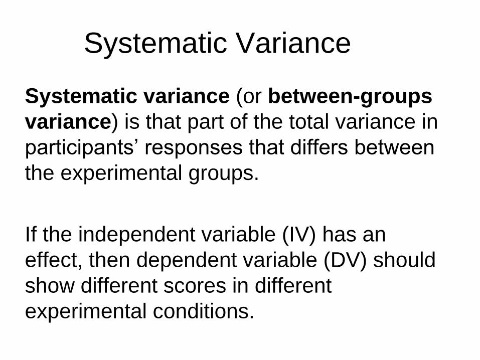
Systematic Variance

Systematic variance (or between-groups

variance) is that part of the total variance in

participants’ responses that differs between

the experimental groups.

If the independent variable (IV) has an

effect, then dependent variable (DV) should

show different scores in different

experimental conditions.

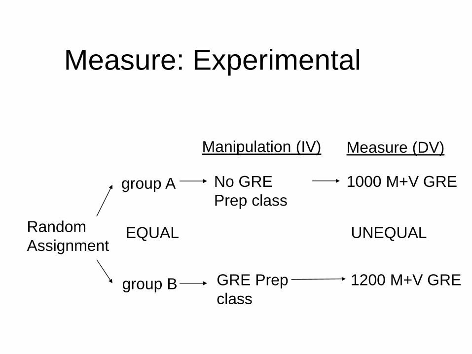
Measure: Experimental

Random

Assignment

group A

group B

EQUAL

No GRE

Prep class

GRE Prep

class

Manipulation (IV) Measure (DV)

1000 M+V GRE

1200 M+V GRE

UNEQUAL

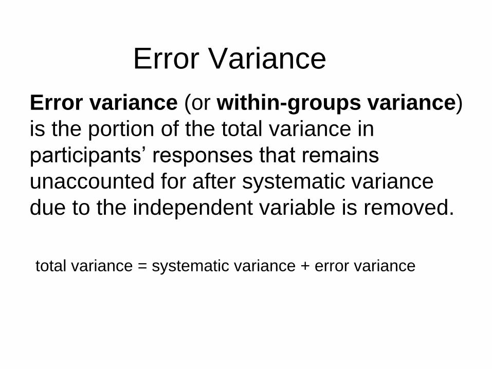
Error variance (or within-groups variance)

is the portion of the total variance in

participants’ responses that remains

unaccounted for after systematic variance

due to the independent variable is removed.

total variance = systematic variance + error variance

Error Variance

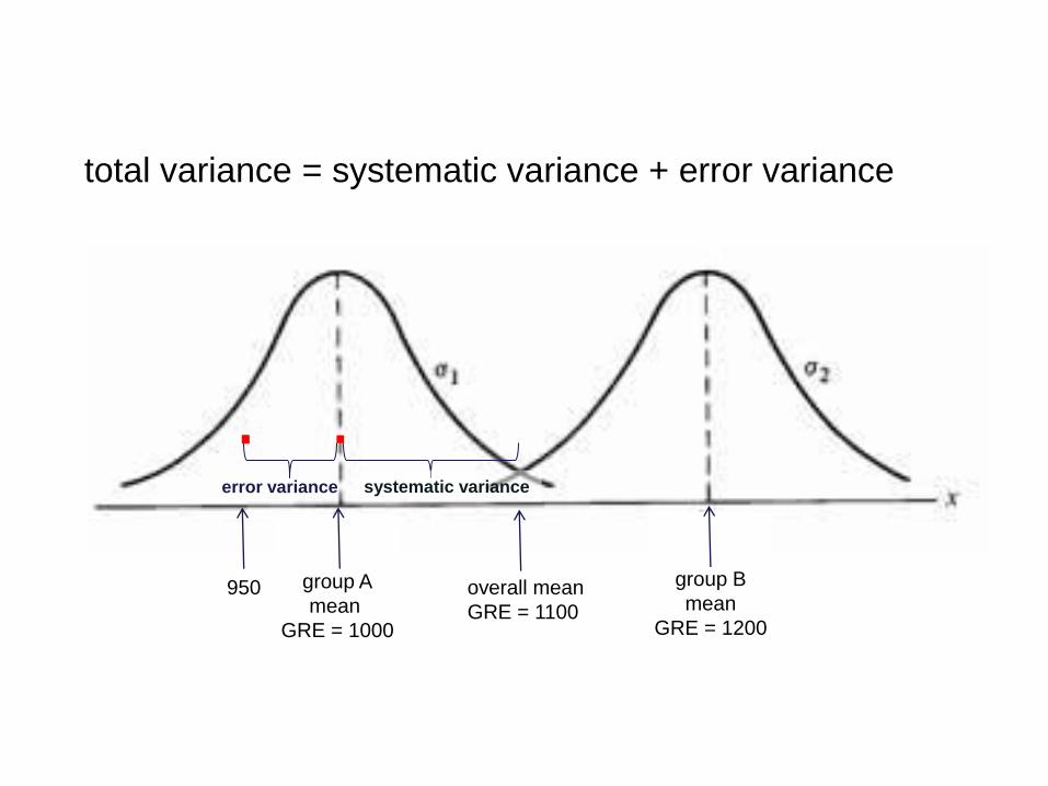
group A

mean

GRE = 1000

group B

mean

GRE = 1200

total variance = systematic variance + error variance

overall mean

GRE = 1100

. error variance systematic variance

. .

950

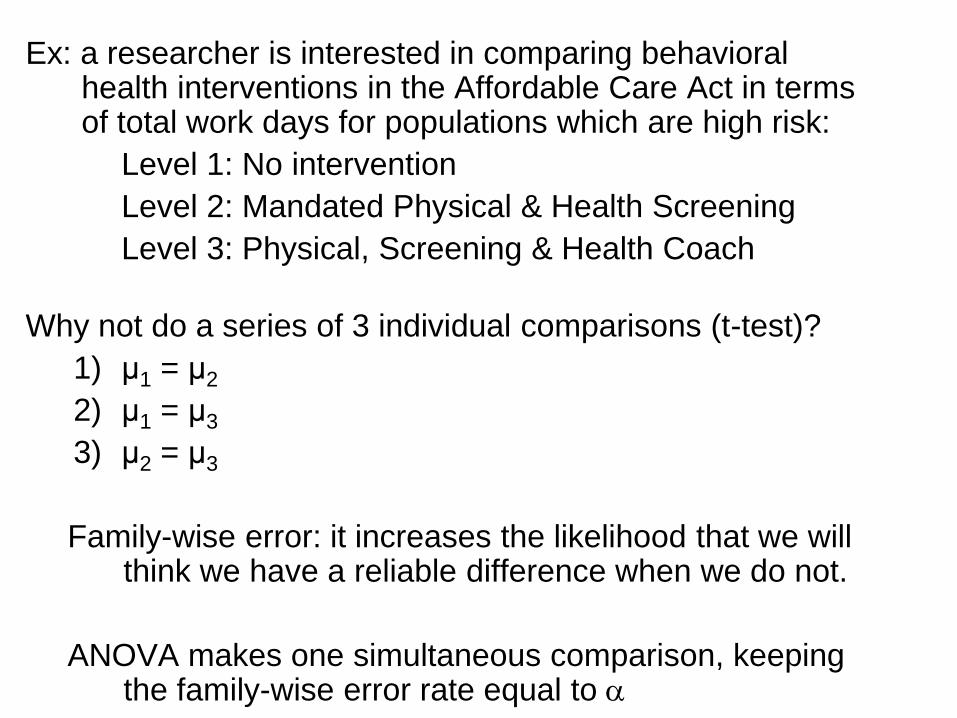
Ex: a researcher is interested in comparing behavioral health interventions in the Affordable Care Act in terms of total work days for populations which are high risk:

Level 1: No intervention

Level 2: Mandated Physical & Health Screening

Level 3: Physical, Screening & Health Coach

Why not do a series of 3 individual comparisons (t-test)?

1) μ1 = μ2

2) μ1 = μ3

3) μ2 = μ3

Family-wise error: it increases the likelihood that we will think we have a reliable difference when we do not.

ANOVA makes one simultaneous comparison, keeping the family-wise error rate equal to a

7

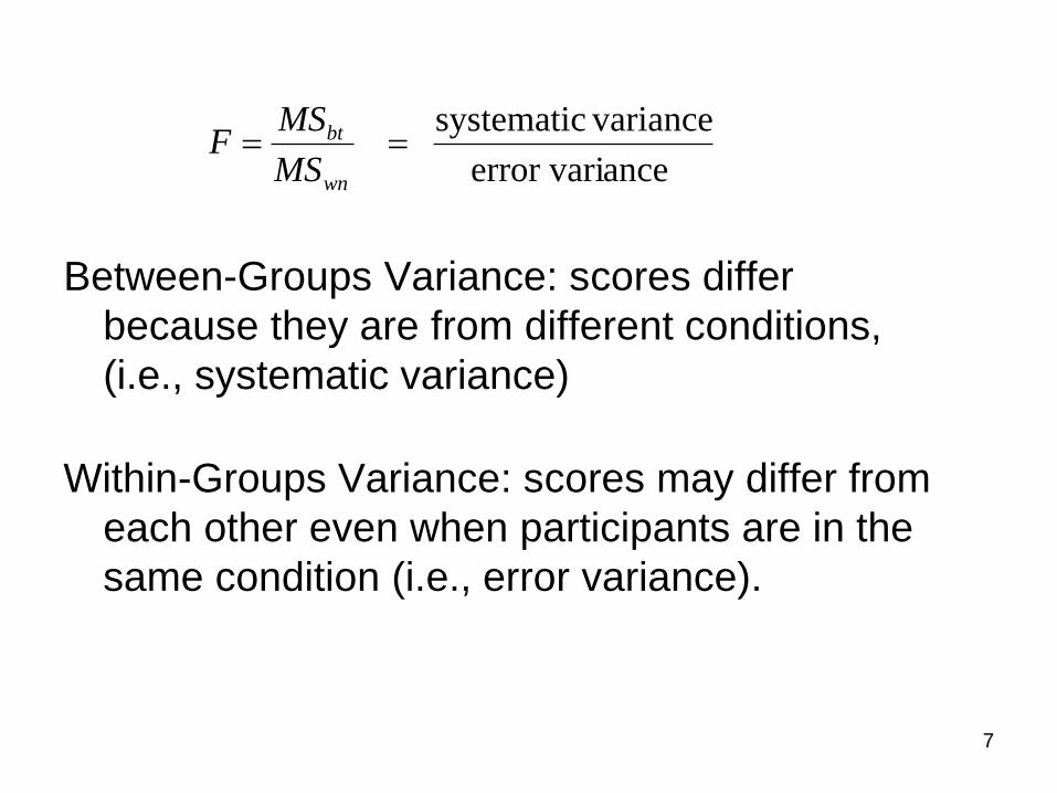
Between-Groups Variance: scores differ

because they are from different conditions,

(i.e., systematic variance)

Within-Groups Variance: scores may differ from

each other even when participants are in the

same condition (i.e., error variance).

anceerror vari

variancesystematic

wn

bt

MS

MSF

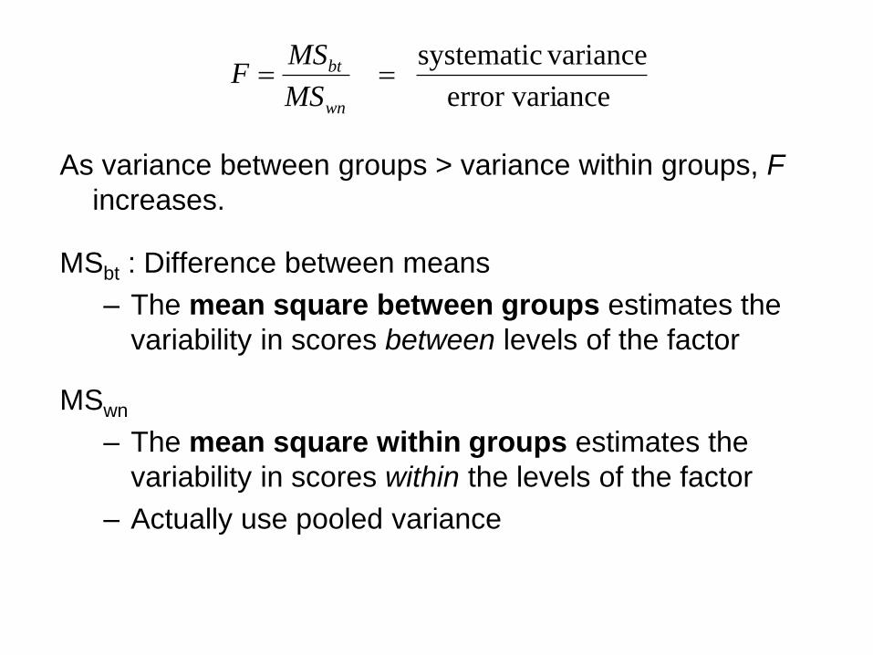
As variance between groups > variance within groups, F

increases.

MSbt : Difference between means

– The mean square between groups estimates the

variability in scores between levels of the factor

MSwn

– The mean square within groups estimates the

variability in scores within the levels of the factor

– Actually use pooled variance

anceerror vari

variancesystematic

wn

bt

MS

MSF

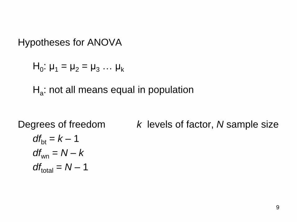
Hypotheses for ANOVA

H0: μ1 = μ2 = μ3 … μk

Ha: not all means equal in population

Degrees of freedom k levels of factor, N sample size

dfbt = k – 1

dfwn = N – k

dftotal = N – 1

9

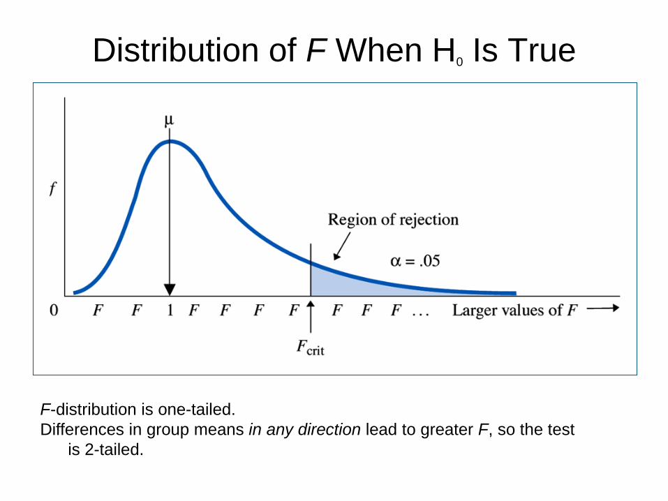
Distribution of F When H0 Is True

F-distribution is one-tailed.

Differences in group means in any direction lead to greater F, so the test

is 2-tailed.

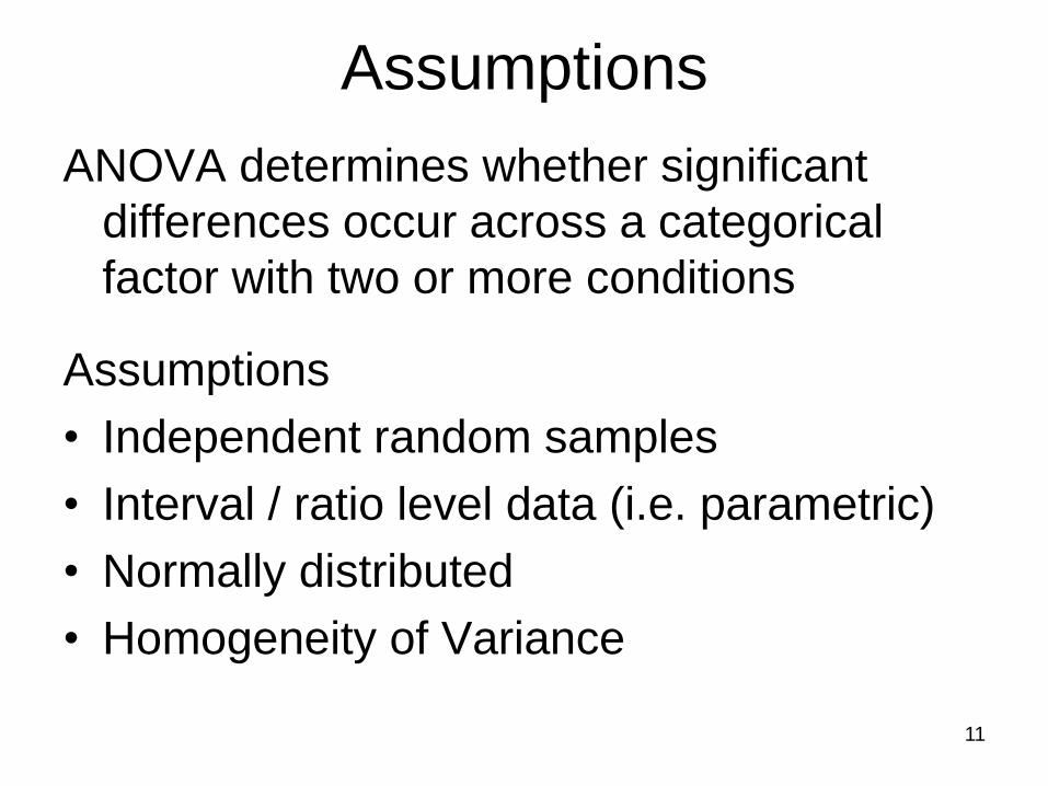
Assumptions

ANOVA determines whether significant

differences occur across a categorical

factor with two or more conditions

Assumptions

• Independent random samples

• Interval / ratio level data (i.e. parametric)

• Normally distributed

• Homogeneity of Variance

11

Breaking it down

12 wnbttotal

wnbttotal

wn

wnw

bt

btbt

wn

bt

dfdfdf

SSSSSS

df

SSMS

df

SSMS

MS

MSF

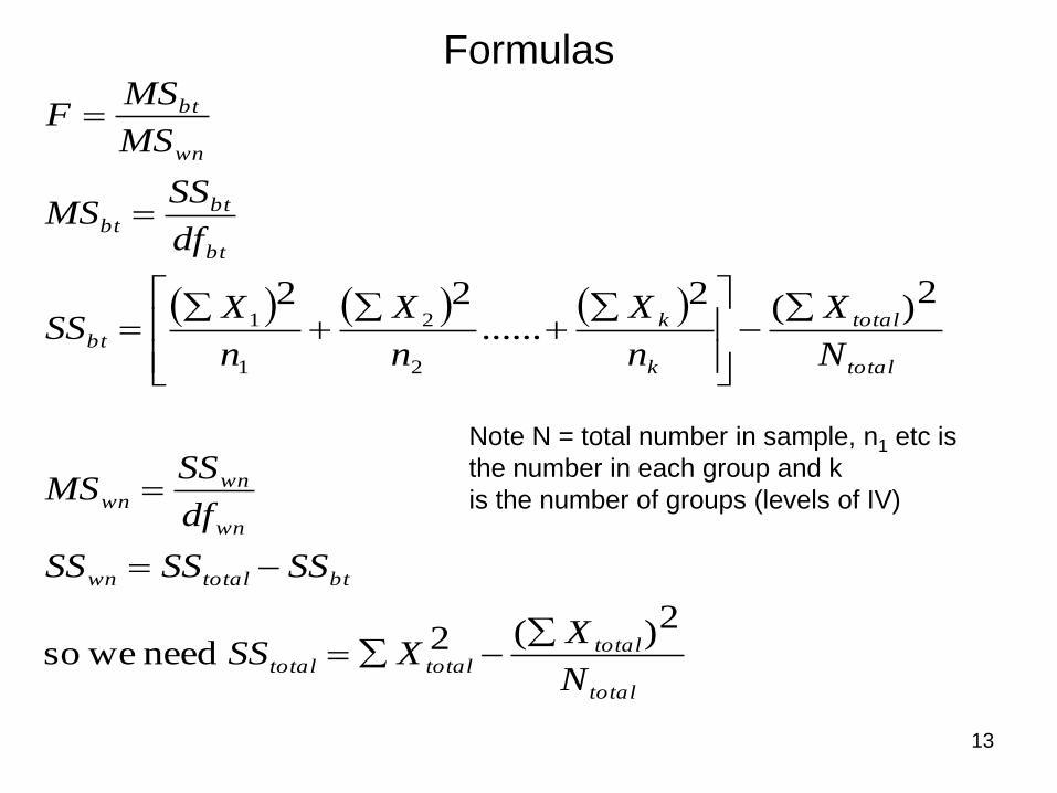
Formulas

13

2)(2 need weso

2)(2......

22

2

2

1

1

total

totaltotaltotal

bttotalwn

wn

wnwn

total

total

k

kbt

bt

btbt

wn

bt

N

XXSS

SSSSSS

df

SSMS

N

X

n

X

n

X

n

XSS

df

SSMS

MS

MSF

Note N = total number in sample, n1 etc is

the number in each group and k

is the number of groups (levels of IV)

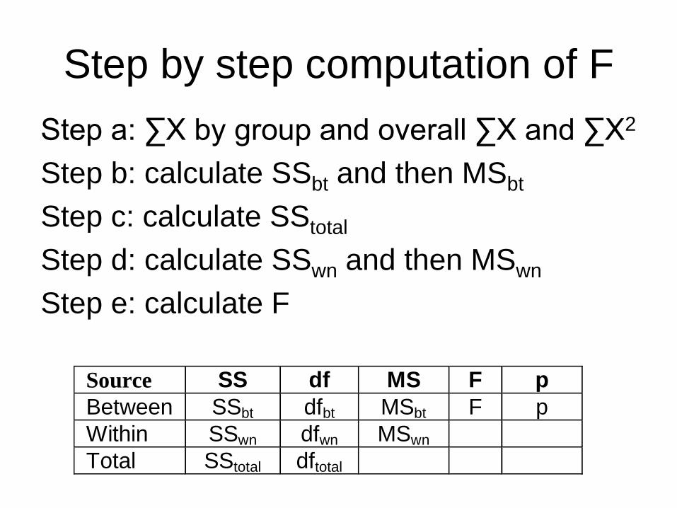
Step by step computation of F

Step a: ∑X by group and overall ∑X and ∑X2

Step b: calculate SSbt and then MSbt

Step c: calculate SStotal

Step d: calculate SSwn and then MSwn

Step e: calculate F

Source SS df MS F p

Between SSbt dfbt MSbt F p

Within SSwn dfwn MSwn

Total SStotal dftotal

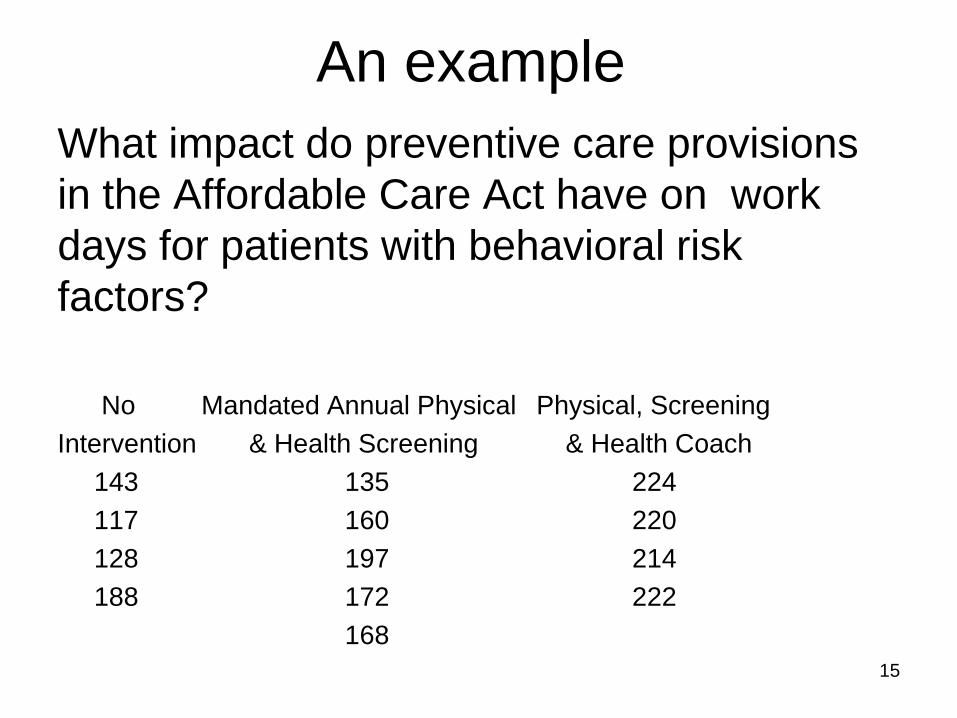
An example

What impact do preventive care provisions

in the Affordable Care Act have on work

days for patients with behavioral risk

factors?

No Mandated Annual Physical Physical, Screening

Intervention & Health Screening & Health Coach

143 135 224

117 160 220

128 197 214

188 172 222

168

15

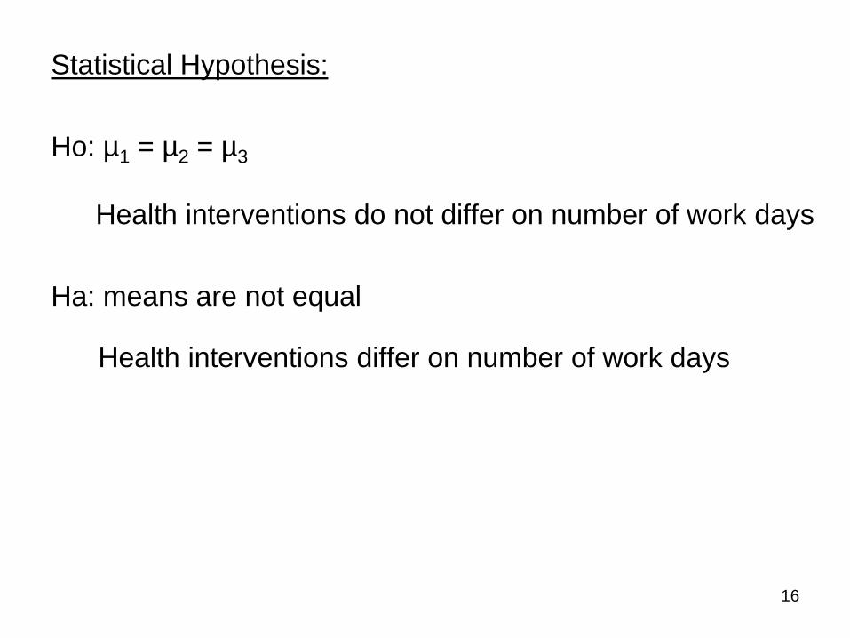
Statistical Hypothesis:

Ho: µ1 = µ2 = µ3

Health interventions do not differ on number of work days

Ha: means are not equal

Health interventions differ on number of work days

16

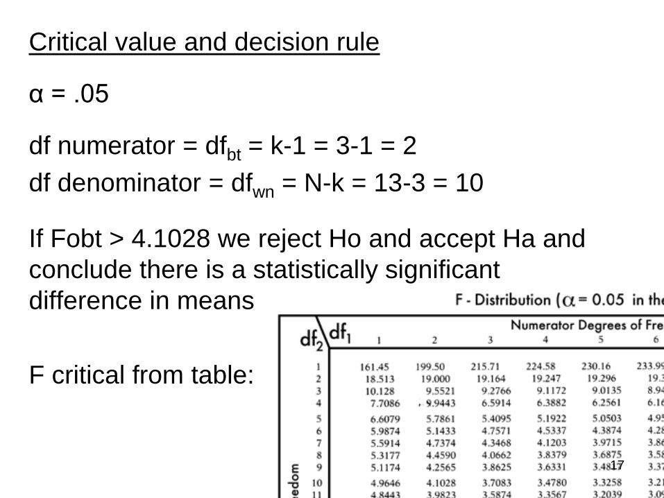
Critical value and decision rule

α = .05

df numerator = dfbt = k-1 = 3-1 = 2

df denominator = dfwn = N-k = 13-3 = 10

If Fobt > 4.1028 we reject Ho and accept Ha and

conclude there is a statistically significant

difference in means

F critical from table:

17

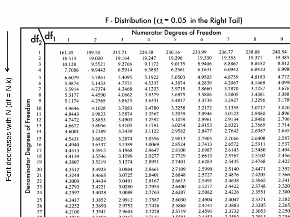
Fcrit decre

ases w

ith N

(df

= N

-k)

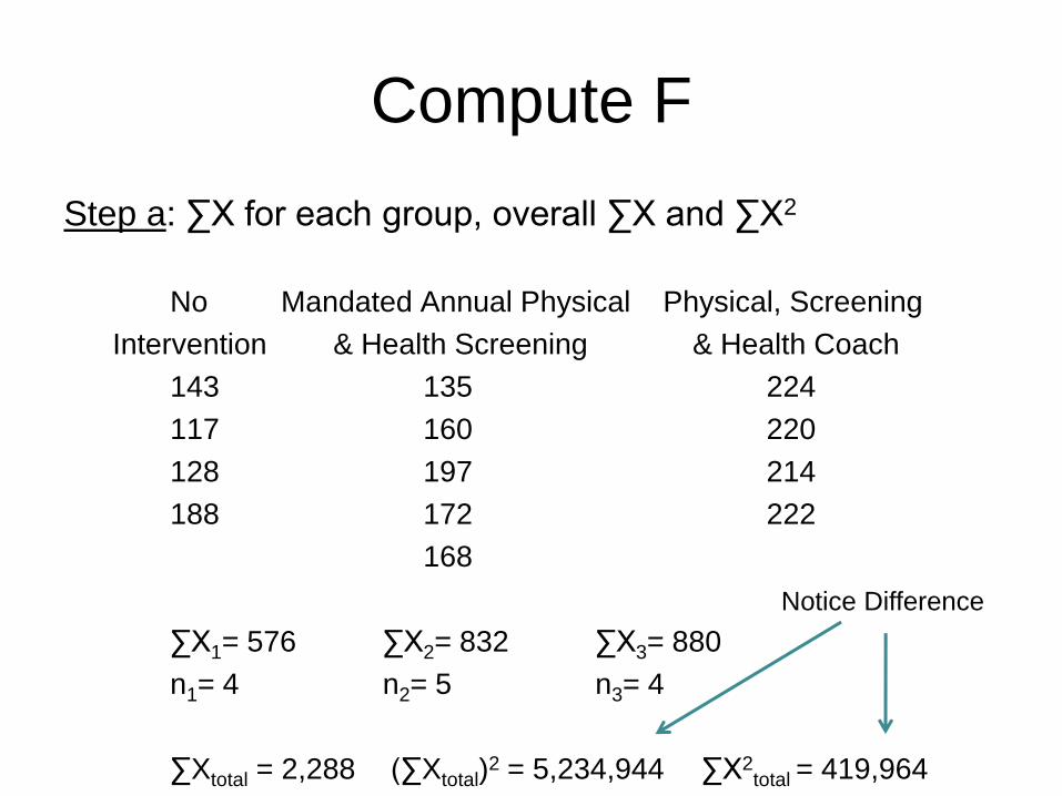
Compute F

Step a: ∑X for each group, overall ∑X and ∑X2

No Mandated Annual Physical Physical, Screening

Intervention & Health Screening & Health Coach

143 135 224

117 160 220

128 197 214

188 172 222

168

∑X1= 576 ∑X2= 832 ∑X3= 880

n1= 4 n2= 5 n3= 4

∑Xtotal = 2,288 (∑Xtotal)2 = 5,234,944 ∑X2

total = 419,964

Notice Difference

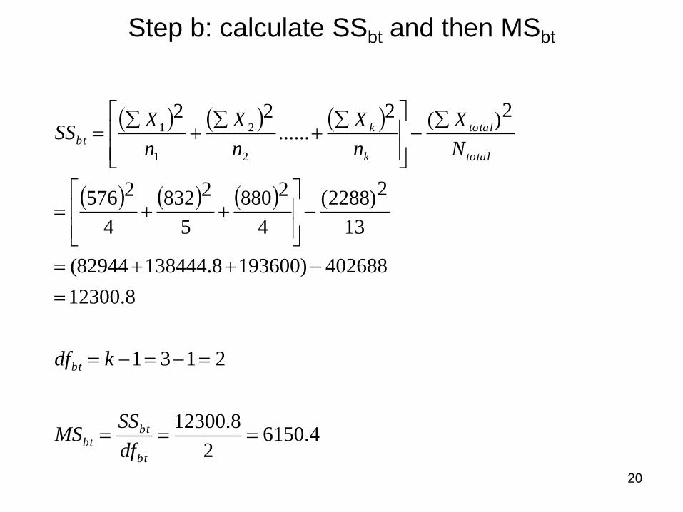
Step b: calculate SSbt and then MSbt

20

4.61502

8.12300

2131

8.12300

402688)1936008.13844482944(

13

2)2288(

4

2880

5

2832

4

2576

2)(2......

22

2

2

1

1

bt

btbt

bt

total

total

k

kbt

df

SSMS

kdf

N

X

n

X

n

X

n

XSS

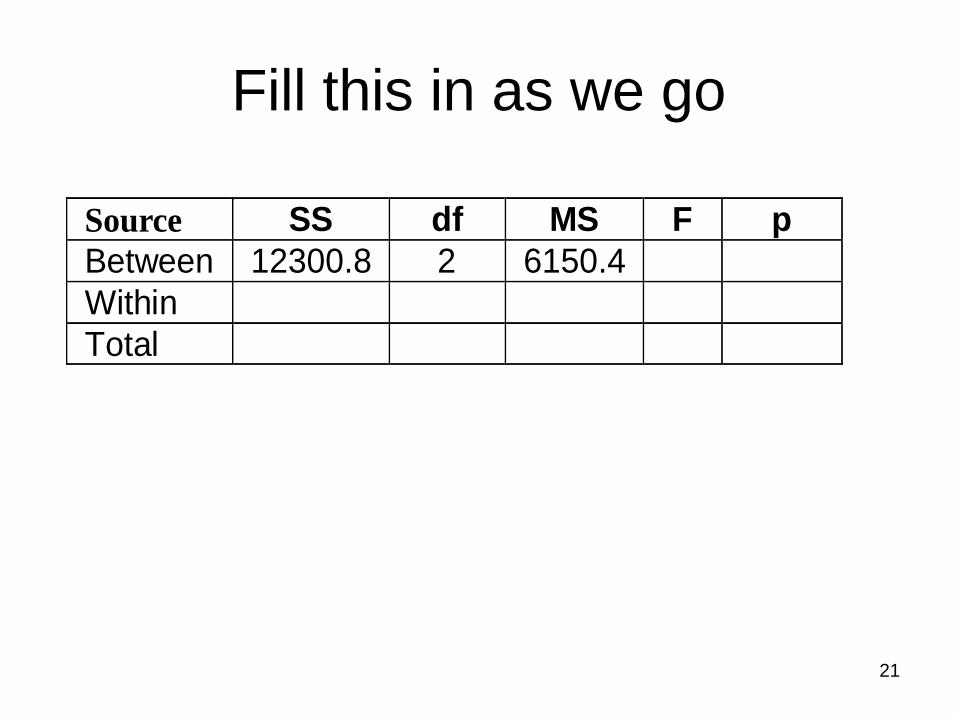
Fill this in as we go

21

Source SS df MS F p

Between 12300.8 2 6150.4

Within

Total

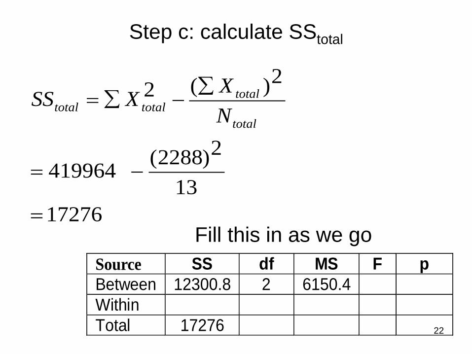
Step c: calculate SStotal

22

17276

13

2)2288( 419964

2)(2

total

totaltotaltotal

N

XXSS

Fill this in as we go

Source SS df MS F p

Between 12300.8 2 6150.4

Within

Total 17276

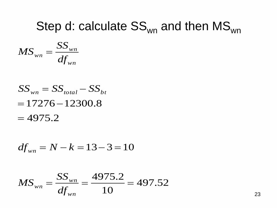
Step d: calculate SSwn and then MSwn

23

52.49710

2.4975

10313

2.4975

8.1230017276

wn

wnwn

wn

bttotalwn

wn

wnwn

df

SSMS

kNdf

SSSSSS

df

SSMS

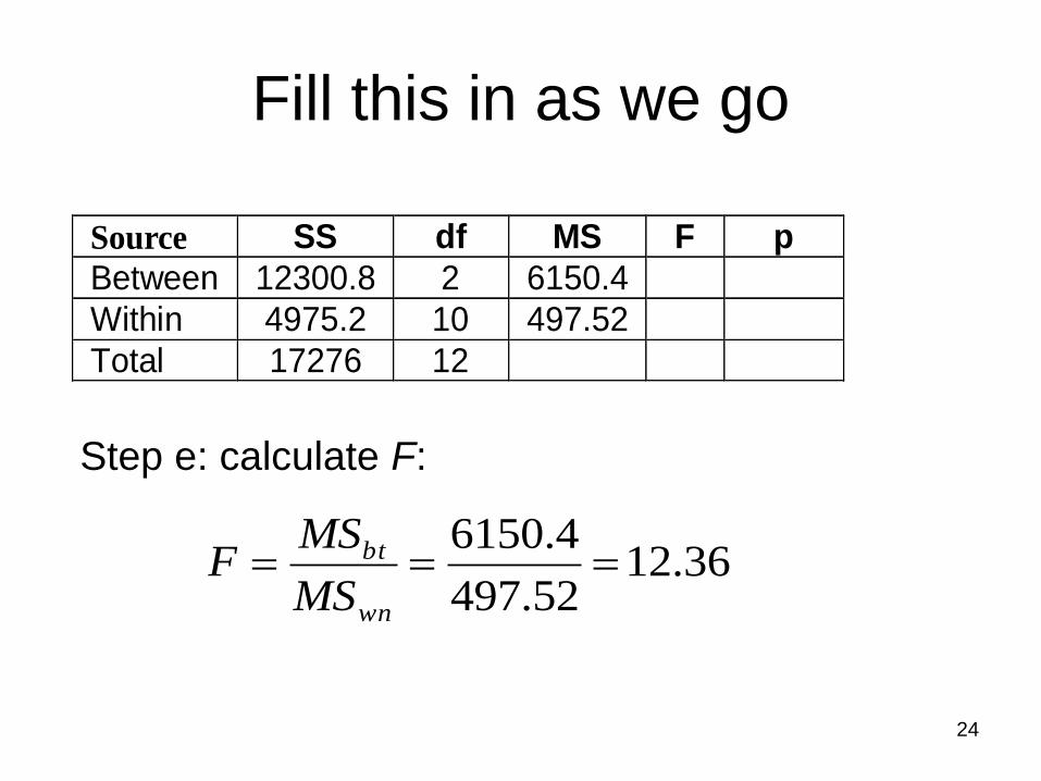
Fill this in as we go

24

Source SS df MS F p

Between 12300.8 2 6150.4

Within 4975.2 10 497.52

Total 17276 12

36.1252.497

4.6150

wn

bt

MS

MSF

Step e: calculate F:

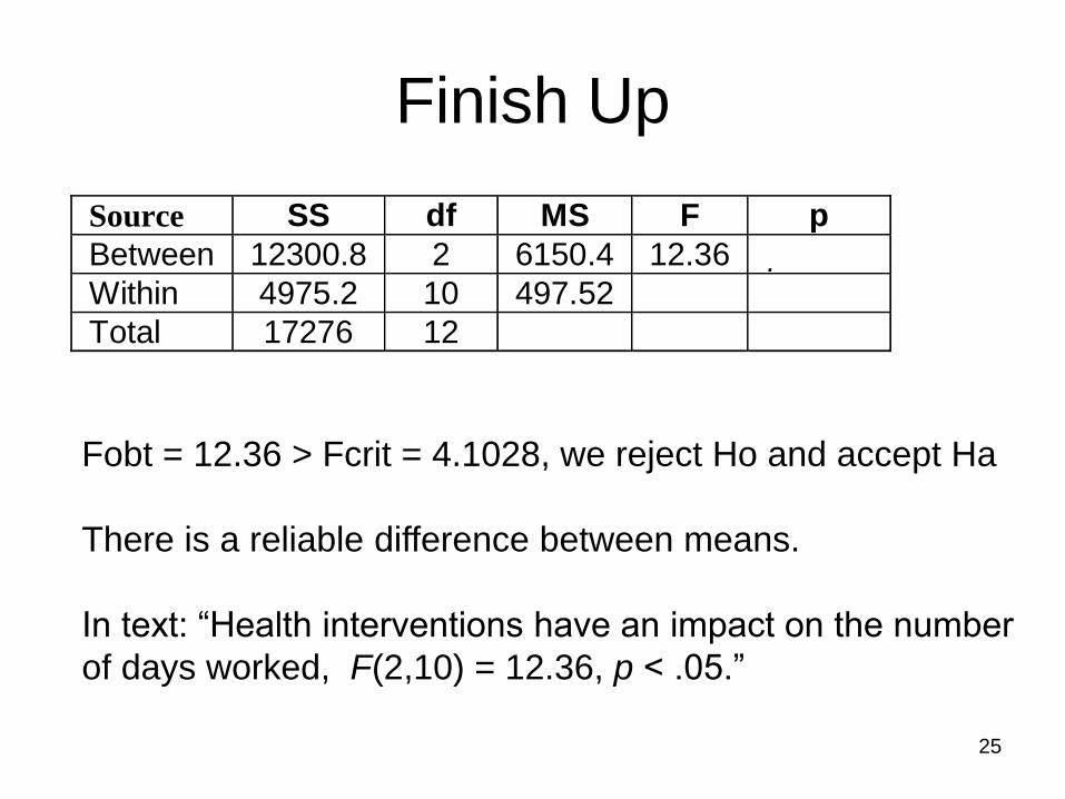
Finish Up

25

Source SS df MS F p

Between 12300.8 2 6150.4 12.36 p < .05

Within 4975.2 10 497.52

Total 17276 12

Fobt = 12.36 > Fcrit = 4.1028, we reject Ho and accept Ha

There is a reliable difference between means.

In text: “Health interventions have an impact on the number

of days worked, F(2,10) = 12.36, p < .05.”

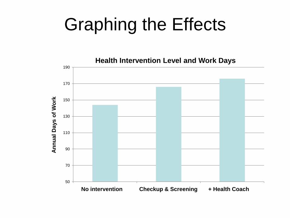
Graphing the Effects

50

70

90

110

130

150

170

190

Job Loss Family Loss Survivor

Health Intervention Level and Work Days

No intervention Checkup & Screening + Health Coach

An

nu

al

Da

ys

of

Wo

rk

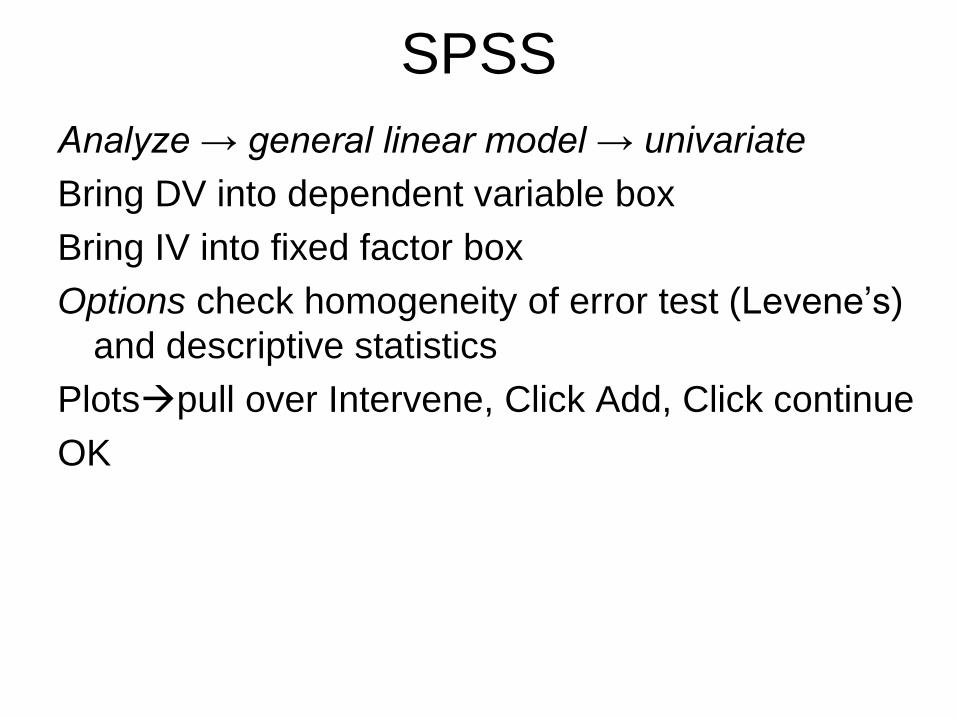
SPSS

Analyze → general linear model → univariate

Bring DV into dependent variable box

Bring IV into fixed factor box

Options check homogeneity of error test (Levene’s)

and descriptive statistics

Plotspull over Intervene, Click Add, Click continue

OK

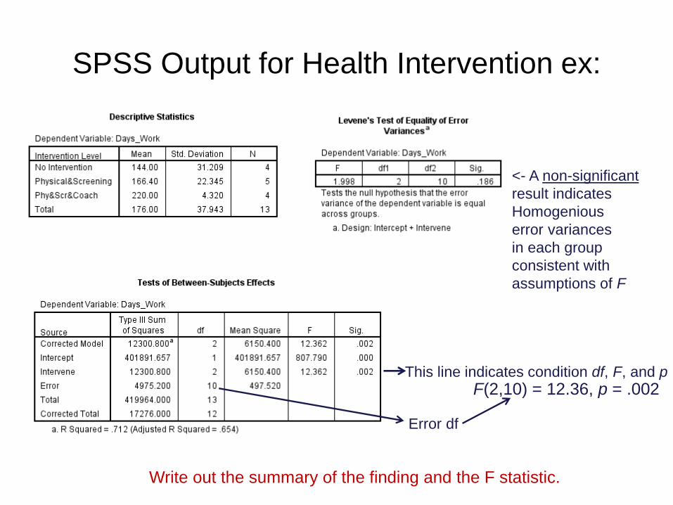
SPSS Output for Health Intervention ex:

<- A non-significant

result indicates

Homogenious

error variances

in each group

consistent with

assumptions of F

This line indicates condition df, F, and p

Error df

F(2,10) = 12.36, p = .002

Write out the summary of the finding and the F statistic.

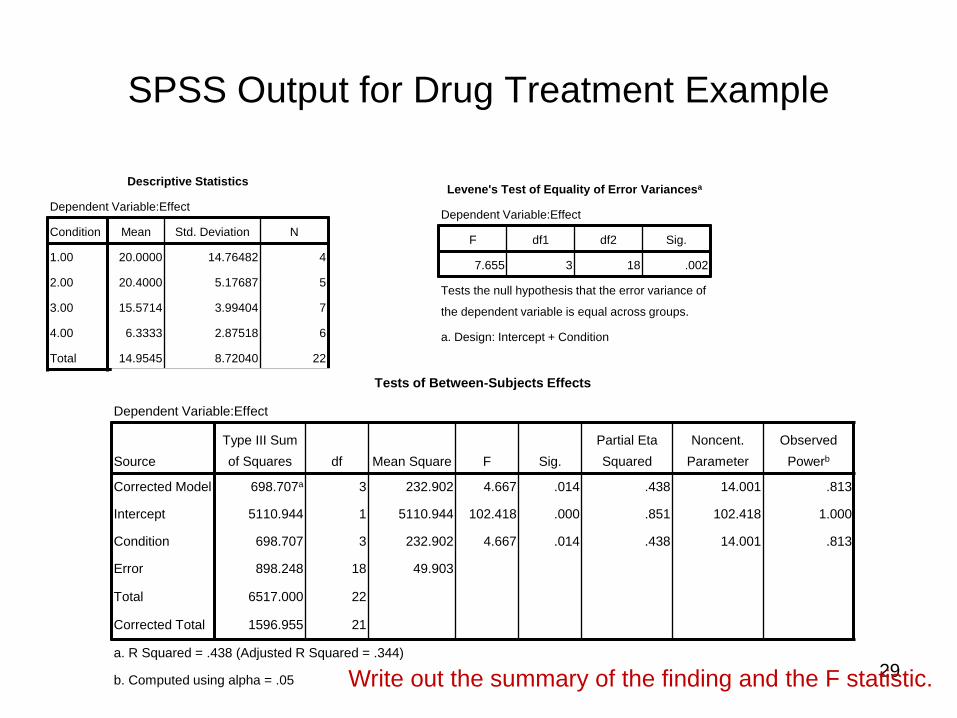
SPSS Output for Drug Treatment Example

Descriptive Statistics

Dependent Variable:Effect

Condition Mean Std. Deviation N

1.00 20.0000 14.76482 4

2.00 20.4000 5.17687 5

3.00 15.5714 3.99404 7

4.00 6.3333 2.87518 6

Total 14.9545 8.72040 22

29

Levene's Test of Equality of Error Variancesa

Dependent Variable:Effect

F df1 df2 Sig.

7.655 3 18 .002

Tests the null hypothesis that the error variance of

the dependent variable is equal across groups.

a. Design: Intercept + Condition

Tests of Between-Subjects Effects

Dependent Variable:Effect

Source

Type III Sum

of Squares df Mean Square F Sig.

Partial Eta

Squared

Noncent.

Parameter

Observed

Powerb

Corrected Model 698.707a 3 232.902 4.667 .014 .438 14.001 .813

Intercept 5110.944 1 5110.944 102.418 .000 .851 102.418 1.000

Condition 698.707 3 232.902 4.667 .014 .438 14.001 .813

Error 898.248 18 49.903

Total 6517.000 22

Corrected Total 1596.955 21

a. R Squared = .438 (Adjusted R Squared = .344)

b. Computed using alpha = .05 Write out the summary of the finding and the F statistic.