Analysis of Two-Well Tracer Tests with a Pulse Input.
152
I40 RHO-BW-CR-131 P Analysis of Two-Well Tracer I. Tests With a Pulse Input Lynn W. Gelhar, Consultant Prepared for Rockwell Hanford Operations, a Prime Contractor to the United States Department of Energy Under Contract DE-AC06-77RL01030 K> ~~~91 9210150247 920914 i PDR WASTE PDR I441 Rockwell International Rockwell Hanford Operations Energy Systems Group Richland, WA 99352 A a. I . M. -I
Transcript of Analysis of Two-Well Tracer Tests with a Pulse Input.

I40RHO-BW-CR-131 P
Analysis of Two-Well Tracer
I. Tests With a Pulse Input
Lynn W. Gelhar, Consultant
Prepared for Rockwell Hanford Operations,a Prime Contractor to theUnited States Department of EnergyUnder Contract DE-AC06-77RL01030
K> ~~~91
9210150247 920914i PDR WASTE PDRI441
Rockwell InternationalRockwell Hanford OperationsEnergy Systems GroupRichland, WA 99352
A a. I . M. - I

Rockwell InternationalRockwell Hanford Operations
Energy Systems GroupRichland, WA 99352
DISCLAIMER
This report was pnrepamd as an account of work sponsored by an agency of the United StatesGovernment. Neither the United States Government nor any agency thereof, nor any of theiremployees, makes any warranty, express or implied. Or assumes env legal liability or respones.bilitv for the accuracy, completeness. or usefulness of any information. apparatus, product. orprocess disclosed, or represents that its use would not infringe privately owned rights. Refer-ence herein to any specific commercial product, process. of service by trade name, trademark.manufacturer, or otherwise, does not necessarily constitute or imply its endorsement, recom-mendation, or favoring by the United States Government or any agency thereof. The viewsano opnions of authors expressed herein do not necessarily state or reflect those of the UnitedStates Government or any agency thereof.
K>
RHO-BW-CR-131 P
K>
.sANALYSIS OF TWO-WELL TRACER TESTS
WITH A PULSE INPUT
Lynn W. Gelhar, ConsultantCambridge, Massachusetts
April 1982
Prepared for the United StatesDepartment of Energy UnderContract DE-AC06-77RL01030
Rockwell IntemationalMOWe NaMord OperaUbta
IANwY Sysmiw am"uP.O. 6ox go0
ftdid. Wilson 30932

RHO-BW-CR-131 P
SUMMARY
Dispersion of a conservative solute, which Is Introduced as a pulse in
the recharge well of a two-well flow system, is analyzed using the general
theory for longitudinal dispersion in nonuniform flow along streamlines.
Results for the concentration variation at the pumping well are developed
using numerical integration, and are presented in the form of dimensionless
type-curves, which can be used to design and analyze tracer tests.
Application of the results is Illustrated by analyzing the preliminary
tracer test run at boreholes DC-718 on the Hanford Site by Science
Applications, Inc., a subcontractor to Rockwell Hanford Operations, in
December 1979.
111

RHO-BW-CR-131 P
CONTENTS
1.0 General Theory . . . . . . . . . . . . .
2.0 Evaluation of Flow Integrals andWell Concentrations . . . . . . . . . . .
3.0 Results . . . . . . . . . . . . . ....
4.0 Application Methodology . . . . . . . . .
5.0 Comments and Recommendations. . . . . . .
* 0 S * S S 0 0 5 * * * I
* 0 * 0 5 * 0 * 0 a S S 0 3
* S S S 0 * S 0 0 5 0 5 4
* . . 0 6 5 6 0 5 0 5 0 12
*. 0 0 0 5 0 0 0 * * . 14
.0
!
6.0 References . . . . . . . . . . . . . . . . . ... 150 * *** ** S
APPENDICES:
FIGUF
A. r and w for Equal Flow Case . . . . . . . .B. Graphic Evaluation of x and X . . . . . . .C. Listing of FORTRAN Program for Numerical
Integration of Equation 4 . . . . . . . . .O. Tables of Type-Curve Data . . . . . . . . .E. Science Applications, Inc. Tracer Test
Data in Boreholes DC-7/8 . . . . . . . . . .
ZES:
1. Streamline Pattern for Two-Well FlowSystem with Q/Qr - 2/3 . . . . . . . . ... .
2. Dimensionless Traveltime Function . . . . .3. Comparison of Exact and Graphic Flow Net
Calculations ...............4. Comparison of Exact Calculation With
Approximation Using Equation B2. . . . . . .S. Effect of Integration Increment. . . . . . .6. Type-Curves for Two-Well Pulse Input Test
With Equal Flow . . . . .. . . . . .7. Type-Curve for Two-Well Pulse Input When the
Recharge Rate is Two-Thirds of the DischargeRate, Q .................. 0 a *
8. Pulse Input Type-Curves PlottedWith Linear Scales . . . . . . . . . . . . .
9. Type-Curve Matching . . . . . . . . . . . .
A-1
C-1* 0 0 0 0 0 * 0-1
................E-1
. . S � � S S �
0 0 0 � 0 * � S
* *. . S 0 S 0
. . . . *. . . .
a * * a . . .
25
6
7a
9
10
. . . . . . & . .
a S 0 0 0 5 0 a 5
....... ........ 11
: . . . . .0 . 0. *. 1
v

RHO-BW-CR-131 P
1.0 GENERAL THEORY
The objective of this analysis is to describe the tracer concentrationwhich evolves in the pumping well of a two-well (pumping-recharge) flowsystem (Fig. 1) when an instantaneous pulse (slug) of conservative tracer isintroduced in the recharge well. The streamline pattern for steady flow ina homogeneous confined aquifer is used in conjunction with the generaltheoretical results of Gelhar and Collins (1971) for longitudinal dispersionin nonuniform flows. With a pulse input their general result for theconcentration, c, is:
c(st) U u(s0 ).iri exp -n(1)
where
s = distance along streamline
t time
a longitudinal dispersivity
n T(S) - t
s'T(s) ' f ds/u(s), traveltime to s
SO
w(t) - f ds/Cu(s)J 2
s(t) = mean location of the pulse at time, t
u(s) - seepage velocity
m a mass of tracer per net area of aquifer injected at s zs- at time, t =O.
1

RHO-BW-CR-131 P
PUMPING RECHARGEWELL WELL RCP8305-30
FIGURE 1.with Q/Qr
Streamline Pattern for= 2/3.
Two-Well Flow System
Equation 1 is applied along each streamline identified by the value ofthe stream function, 4'; therefore the velocity, u, depends on 1, and as aresult, T(s, 4) and w(t, p). These flow integrals can be evaluated eitheranalytically or graphically as described in the next section. The coeffi-cient m/u(so) in Equation 1 is evaluated by noting that at the recharge well:
u(so) - Qr/( 2wrwnH)
Qr recharge rate
rw = well radius
n = effective porosity
H = aquifer thickness
m = M/2wrwnH
M = mass of tracer injected
m/u(s 0) = M/Qr
2
RHO-BW-CR-131 P
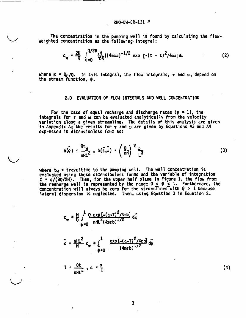
The concentration in the pumping well is found by calculating the flow-weighted concentration as the following. integral:
c 2H fQ/2H(M)(4w=)e1/2xp [-( - t) /4=]d (2)
where B ' Qr/Q. In this integral, the flow integrals, T and w, depend onthe stream function, 4.
2.0 EVALUATION OF FLOW INTEGRALS AND WELL CONCENTRATION
For the case of equal recharge and discharge rates (B - 1), theintegrals for T and w can be evaluated analytically from the velocityvariation along a given streamline. The details of this analysis are givenin Appendix A; the results for T and w are given by Equations A3 and A4expressed in dimensionless form as:
a(¢) = , b(s,*)='(- 2 (3nHL L
where tw c traveltime to the pumping well. The well concentration isevaluated using these dimensionless forms and the variable of integrationV - */(BQ/2H). Then, for the upper half plane in Figure 1, the flow fromthe recharge well is represented by the range 0 < V < 1. Furthermore, theconcentration will always be zero for the streamTines with 0 1 becauselateral dispersion is neglected. Then, using Equation 3 in Equation 2,
M 1 Q.exp -(a-T)2/4eb] dAcw, ZI 2 172nL(4ireb)
nHL2 1 exnt-fa T)2/4d,1AC Z -wr CW C I e t-(aT b do
CO ~(4rc b)
T Qt C Er (4)nHL
K>
3
RHO-BW-CR-131 P
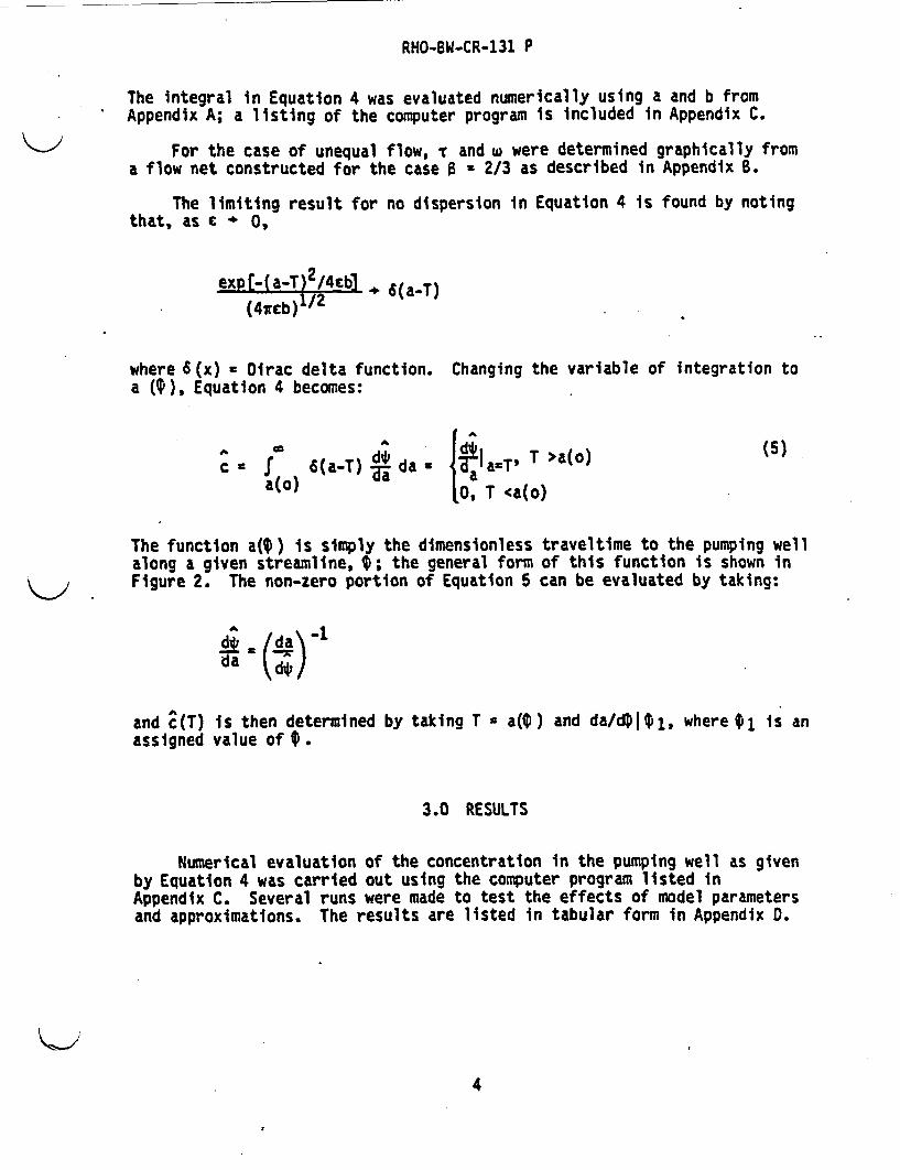
The integral in Equation 4 was evaluated numerically using a and b fromAppendix A; a listing of the computer program is included in Appendix C.
For the case of unequal flow, i and w were determined graphically froma flow net constructed for the case 0 - 2/3 as described in Appendix B.
The limiting result for no dispersion in Equation 4 is found by notingthat, as E * 0,
expf-(a-T 2/4cb] * 6(a-T
(4wcb) /2
where 6(x) = Dirac delta function.a (iT), Equation 4 becomes:
Changing the variable of integration to
A f0
a(o)6(a-T) Ka da C TlacT' T >a(o)
0, T <a(o)
(5)
The function a(Q) is simply the dimensionless traveltime to the pumping wellalong a given streamline, $; the general form of this function is shown inFigure 2. The non-zero portion of Equation 5 can be evaluated by taking:
A (dao -1
da (;and c(T)assigned
is then determined by taking T a(V ) and da/d*q1$, where t1value of V.
is an
3.0 RESULTS
Numerical evaluation of the concentration in the pumping well as givenby Equation 4 was carried out using the computer program listed inAppendix C. Several runs were made to test the effects of model parametersand approximations. The results are listed in tabular form in Appendix 0.
4

RHO-BW-CR-131 P
The integral in Equation 4 was evaluated numerically using a and b fromAppendix A; a listing of the computer program is included in Appendix C.
For the case of unequal flow, T and w were determined graphically froma flow net constructed for the case 0 - 2/3 as described in Appendix B.
The limiting result for no dispersion in Equation 4 is found by notingthat, as c * 0,
exp[-(a-T)2/4EbI * 6(a-T)
(4wffcb) 112
where S(x) = Dirac delta function.a (Vt), Equation 4 becomes:
Changing the variable of integration to
cu fa(o)
&(a-T) Si da - dl a=T, T >a(o)
0, T <a(o)
(5)
The function a(¢) is simply the dimensionless traveltime to the pumping wellalong a given streamline, i; the general form of this function is shown inFigure 2. The non-zero portion of Equation 5 can be evaluated by taking:
A -Oa di/
and c(T)assigned
is then determined by taking T = a (t ) and da/d|Iq 1, where $t i is anvalue of V.
3.0 RESULTS
Numerical evaluation of the concentration in the pumping well as givenby Equation 4 was carried out using the computer program listed inAppendix C. Several runs were made to test the effects of model parametersand approximations. The results are listed in tabular form in Appendix D.
K>
4

RHIO-BW-CR-131 P
<a3 0.5
0I0 1 2 3 4 5
A
(WI RCPS305-31
FIGURE 2. Dimensionless Traveltime Function.
Figure 3 shows a comparison of the graphically based results usingm I (Appendix B) and the exact result using the equations from Appendix A.The excellent agreement demonstrates the adequacy of the graphicapproximation with m - 1 In Equation 52; that value was used in allsubsequent calculations. Figure 4 illustrates the effect of using theapproximate form of Equation 62; some difference is observed at lowerconcentrations for the rising limb of the curve with the large value ofc * 0.2. For smaller c, the differences are generally smaller, as shown inFigure 3. The effects the increment, AV, used to approximate the integralin Equation 4 are illustrated in Figure 5. When E = 0.01, the largerAt = 0.05 produces oscillations in the tail of the curve, but these areeliminated when At * 0.01; for E = 0.2 the results are nonoscillatory whenAV = 0.05. Generally, the oscillations are eliminated if AV < c.
The overall results are summarized in Figures 6 and 7; the unequal flowcase (Fig. 7 with B = 2/3) corresponds to the Science Applications, Inc.tracer test of December 1979. These results show that the dispersionparameter, c a v/L, affects the rising part of the curve and the peak butnot the tail. This point is further demonstrated by the behavior of thenondispersive solution using Equations 5 and AS As shown in Figure 6. Thisshows that all of the results approach the nondispersive analytical resultfor large time, and further demonstrates the adequacy of the numericalprocedure. Generally, the breakthrough curves are characterized by a steeprising limb and an elongated tail, as shown in the linear plots of Figure 8.'The log-log plots (Fig. 6 and 7) are convenient for estimating thedispersivity and effective porosity from tracer test data, as illustrated inthe following section.
5

RHO-BW-CR-131 P
. I
it I
0.o0 LI0.1 0.5 1 5
T -pHI.1
10
RCPS30S-32
FIGURE 3. Comparison of Exact and Graphic Flow Net Calculations.
6

RHO-BW-CR-131 P
I
go
0.5
<a 0.1
0.06
0.01 L_0.1 0.5 I 5
T
10
RCP8305-33
FIGURE 4. Comparison of Exact Calculation With ApproximationUsing Equation B2.
7

RHO-6W-CR-131 P
I
0.5
<0 0.1
0.05
0.01 It0.1 0.6 1 5
T10
RCPa305-34
FIGURE 5. Effect of Integration Increment.
8

RHO-BW-CR-131 P
1-
0.5 _
0.1
0.1 0.5 1 60:
T at-a
la
RCPS305-3S
FIGURE 6. Type-Curves for Two-Well Pulse Input Test With Equal Flow.
9

RHO-BW-CR-131 P
-_
0.5
<U
0.05 _
0.01 _0.1 0.5 1 6
. (tT -
10
RCPS305.36
FIGURE 7. Type-Curve for Two-Well Pulse Input When the RechargeRate is Two-Thirds of the Discharge Rate, Q.
kJ
10

RHO-BW-CR-131 P
- EQUUAL FLOW|_| Lu *0.01. 0.02. 0.05. I
0.01
t 0.5
0.02
0.05
0.2
0 6 lo
T *a RCPS305-37
FIGURE 8. Pulse Input Type-Curves Plotted With Linear Scales.
K>
11

RHO-BW-CR-131 P
4.0 APPLICATION METHODOLOGY
The procedure for interpretation of tracer test data using the resultsof the above analysis is illustrated by analyzing the test conducted byScience Applications, Inc. at DC-7/8 in December 1979. Since some of theconditions of that test were not fully defined, the results of this interpre-tation are considered to be preliminary; this example is present primarilyto illustrate the procedures which can be used to analyze such tests.
The Science Applications, Inc. tests were reanalyzed using the type-curves in Figure 7. The flow rates for the test were estimated using theaverage rates implied for the period 15:13-23:00 (see Appendix E, Table E-4);Qr = 2.31 gal/min (injection rate) and Q - 3.42 gal/min (pumping rate) orQr/Q -B a 2/3. Based on these rates and estimates of the volume in theborehole flow conduits and connecting plumbing, the following traveltimeswithin the tubing to and from the test horizon were estimated:
* Time down in Injection well = 153 min.
* Time up in pumping well * 258 min.
These times were subtracted from the observed times to give the actual elapsedtime since the tracer entered the formation. Also, the elapsed time wascorrected to correspond to a constant pumping rate of 3.42 gal/min, based onthe actual metered volume in Table E-6. After these time corrections weremade, the actual data points in Figure E-2 were plotted with the estimatedbackground of 20 counts subtracted; the corrected data are shown inFigure 9, along with two of the dimensionless type-curves in Figure 7 forB = 2/3. Overlaying the data on the type-curve, we find a reasonable fitfor E in the range 0.02 to 0.05; using e = 0.035 = a/L and L = 56 ft, theindicated longitudinal dispersivity is a 0 9.035(56) = 1.96 ft. Matchingthe time scales in Figure 9, I - 1 * Qt/nHL, t(hours) -.1.18 hr yields theeffective thickness nH = Qt/L - 0.0105 ft.
The data in Figure 9 seem to show some systematic departures from thetheoretical type-curve. This could be a reflection of experimental ambigui-ties such as the following:
1. The background concentration is not clearly determined, and smallchanges in this level could drastically alter the lowconcentration parts of the curve.
2. Unobserved flow rate variations during the period that the tracerwas passing the sensor would distort the shape of the curve.
3. Uncertainty about the volume in the connecting conduits couldintroduce errors in the traveltime correction and alter the shapeof the curves.
12

RHtO-BW-CR-131 P
1.000
500
100
60
J1
10
5
20.1 0.6 1 5
TIME (hrl10
RCP8305.38
FIGURE 9. Type-Curve Matching.
13

RHO-BW-CR-131 P
*The differences in Figure 9 could also indicate that the tested zone doesnot behave as a homogeneous, constant-thickness aquifer. If other sourcesof errors were eliminated, departures on the tail of the curve would bediagnostic of that possibility because that part of the type-curves isdetermined solely by convection; i.e., the traveltime distribution.
Calculations for the Science Applications, Inc. test were also madeusing the approximate method developed in Appendix E. From Figure 9 thepeak time t = 1.5 hr and the time to rise from one-half of the peak ist = C-45 hr. Then using Equation E35 with F = 0.202, G 0.0488 (a = 2/3):
a r 1 F (At) = 0.0271r 41nZ G tZ
p
a = 1.52 ft
and from Equation E22 with Q = 3.42 gal/min:
QtnH = i = 0.0103 ft.
2,1 F
These results show good agreement with those from the type-curve approachand indicate that the approximate method in Appendix E is reliable. Ofcourse, the type-curve method has the advantage, in that it uses thecomplete breakthrough curve.
The type-curves of Figure 6 and 7 can also be used to design tracertests; using estimates of c a a/L, the actual concentration level that willresult from a given mass of tracer M can be determined in terms of theeffective thickness nH and the well spacing L; i.e., cw a Mt/nHL2.
5.0 COMMENTS AND RECOMMENDATIONS
These results demonstrate the feasibility of the two-well tracer testwith a pulse input as a method of determining effective porosity anddispersivity. This type of test has the advantage that the shape of thebreakthrough curve is very sensitive to the dispersivity. This is incontrast to the more frequently used step input (Webster et al., 1970; Groveand Beetem, 1971; Robson, 1974; Mercer and Gonzalez, 1981) in whichdispersion affects the shape of the curve only in the initial lowconcentration portion of the curve.
14

RHO-BW-CR-131 P
The type-curves developed here provide a simple method of designing andanalyzing two-well pulse input tracer tests. I
The method of analysis used here presumes that a/L is relatively small;results in Gelhar and Collins (1971) indicate that the method should bereasonably accurate for v/L < 0.1. If the method is to be used for largervalues of a/L, some comparative testing with numerical solutions issuggested. However, it should be recognized that, under those conditions(large a/L), other factors such as displacement-dependent dispersivity andnon-Ficklan effect (Gelhar et al., 1979) may complicate the interpretation.Also, transverse dispersion is neglected in this analysis; this assumptionis reasonable for small a/L because then the dispersion effect occursprimarily along the more direct streamlines for which the fronts will benearly perpendicular to the streamlines. For larger a/L, the dispersioneffect along a wider range of streamlines becomes important; numericaltesting would also be required in this case. When a/L is large, a finite-difference or finite-element solution should be routine because a relativelycoarse grid could be used.
The type-curves for the pulse input can also be used to treat otherinputs by convolution. In particular, this would apply to recirculatingtests in which the pulse is routed through the aquifer several times. Thisaspect is important in the Hanford tests because analysis of the secondarypeaks would provide a check on the borehole traveltime. Some preliminarywork has been done on numerical convolution of the pulse input results. Itis recommended that this be developed for analysis of the Hanford data.
6.0 REFERENCES
Gelhar, L. W. and M. A. Collins, 1971, "General Analysis of LongitudinalDispersion in Nonuniform Flow," Water Resources Res., 7 (6),pp. 1511-1521.
Gelhar, L. W., A. L. Gutjahr, and R. L. Naff, 1979, "Stochastic Analysis ofMacrodispersion in a Stratified Aquifer," Water Resources Res., 15 (6),pp. 1387-1397.
Grove, D. B. and W. A. Beetem, 1971, "Porosity and Dispersion ConstantCalculations for a Fractured Carbonate Aquifer Using the Two-WellTracer Method," Water Resources Res., 7 (1), pp. 128-134.
Mercer, J. W. and D. Gonzalez, 1981, Geohydrology of the Proposed WasteIsolation Pilot Plant in Southeastern New Mexico, Nei- Mexico GeologicalSociety Special Publication 10, pp. 123-131.
Robson, S. G., 1974, Feasibility of Water-Quality Modelina Illustrated byApplication at Barstow? California, Water Resources Invest. Rep. 46-73,U.S. Geol. Survey, Menlo Park, California, 66 pp.
Webster, D. S., J. F. Proctor, and I. W. Marine, 1970, Two-Well Tracer Testin Fractured Crystalline Rock, U.S. Geol. Survey Water Supply Paper1544-1, 22 pp.
15

RHO-BW-CR-131 P
APPENDIX A
T AND X FOR EQUAL FLOW CSE*. t. '....
A-1

RHO-BW-CR-131 P
APPENDIX A
T AND w FOR THE EQUAL FLOW CASE
When Q u Q it is easily shown that the streamlines are circular arcs..: that case the few is conveniently described in the polar coordinate systemshown in Figure A-1. The piezometric head, h, for steady flow in this systemis:
In
h = Tlk ln(rl/r2)2
Tr a transmissivlty
r21 (x + L)2 + y2, x = -R siny
r2 = (x - L)2 + y2, y - R cosy - 8
and using the Darcy equation, seepage velocity along the streamline is:
. Tr ohy F-NH
i r21;T Sr2
r2 /
After extensive algebraic manipulation, this reduces to:
V C 2QR.sin3t
Y irnHL 2 (cosy - coso)
Using this velocity in the traveltime integral:
(Al)
so
dsuTS)
y=f-
Rdyvy
a i n HL (siny + sin - (y + *)coso)Q 2i 3 (A2)
K>;/
A-2

Ck C (I.
II
A,I
I
f
iI ,
I ,
I .
-.1-1It
I
II
.4t*
I..
'1%
L.
A'p- I Ax0
LA
O-A
'A)
RCP8305-39
FIGURE A-1. Polar Coordinate System for the Equal Flow Case.

RHO-BW-CR-131 P
When y - *, Equation A2 gives the traveltime to the pumping well or:
a(A) . = -A 3I- (sinf - ~cos¢)
AM"VOWUgS % >;:fir - -. - .
(A3)
Equation A3 gives the dimensionless traveltimeof ~; this result is used for a in Equation 4.integral is evaluated from Equation Al as:
between the wells as a functionSimilarly, the w flow
i
so
ds
[u(s)] r=$ VY
1 fL~2 \ 2 b(j, 4)
b(j,*) = [i;2sin_ .
+ siny osy sins cou+ .2
.. uw4,..waaurnmsmptae.in2cos 4t(siTfl 4 sin*) + (y + .)cos 2.] (A4)
Here y indicates the position of the pulse along-the streamline correspondingto * vrl. At a given time the position j is found by solving Equation A2for y = ? when T = t; this is done iteratively using the program listed inAppendix C. When j>, the pulse for a given streamline has moved into thepumpinj well; in this case w (or b in Equation 4) was calculated from Equation A4using y = 0.
If dispersion is neglected, the concentration is found from Equation 5using Equation A3 to find dq/dala=T,
da = ,2 s 2A 3A 2 A ^ 3 4 A
-^ a recc cotw4* + 2w Vcsc irf* cot ir4 + V *csc #4d ip -
(AS)
The. concentration cis then found by assigning values of T between 0 and 1,calculating T = a from Equation A3 and dx/da from Equation AS.
A$W A." " -- -- *.- -
A-4

RHO-BW-CR-131 P
APPENDIX 8
GRAPHIC EVALUATION OF T AND X
K>~~~~~~~ .-... ......
F ----.. --;£,e
B-1

RHO-BW-CR-131 P
APPENDIX B
GRAPHIC EVALUATION OF T AND w-. t v'- -;'}w~k2b'
t .- . w--;* -:
The flow integrals t and w can be determined from a graphic constructionof the streamline pattern. This approach is necessary in the unequal flowcase where the analytical description of the flow field is very complicated.The streamline pattern for Qr/Q a = 2/3 (see Fig. 1) was constructed bystandard superposition of the ray streamlines of the appropriate source andsink strength. If each streamtube has a flow, Qo, and a width, w(s), as afunction of the distance along the centerline of the streamtube, s, the velocityis:
u(s) = Q/(nHw(s))
and then the flow integrals are expressed as:
t mfI ds n H Iod
w ds (nH2 f 2ds
These integrals were approximated by measuring the width of the streamtubesat intervals, As, along each of the streamtubes and summing the appropriatequantities (wAs or w2as). The integrals were evaluated for each streamtubefor intervals in the 4 of 0.1 at the pumping and well normalized as inEquation 3. These data for a (f) and b (I) at the pumping well were thenfit to polynomials of the form:
4n2n
ln b E bn 4, (B1)nro
_ , _ _. _.... ... ~ . -.
B-2

RHO-BW-CR-131 P
These expressions were then used in the integrations of Equation 4 to findthe concentration in the pumping well. Note that Equation B1 gives only thevalue of b at the pumping well bw. In general, b will increase with timeas the pulse approaches the weil along a given streamline; this behavior wasrepresented in the form:
b/by . (T/a)m, T <a (B2)s1, T >a
where m is a positive exponent to be specified. a and b from Equations 61and B2 were then used in Equation 4 to find c.
In order to evaluate the above graphic procedure, the flow netevaluation was done first for the equal flow case B - 1 and the results werecompared with the exact analytical approach in Appendix A.
8-3

RHO-BW-CR-131 P
APPENDIX C
LISTING OF FORTRAN PROGRAM FORNUMERICAL INTEGRATION OF EQUATION 4
C-1

RHO-BW-CR-131 P
C
CCCCcCCCCCCC
CCCcC
CCCCC
CC
ICCC
WellDavid GelharDecember 1981
This program calculates the concentration (Cw) oftracer appearing in a well as a function of the timeelapsed since the tracer was pumped down another well.The user is asked to supply several initializing parameters,and the values of 7 (time) desired. First, the all-purposeparameter epsilon (which accounts for dispersion effects) isinput Then, you are asked to input the last valueof psi and the increment of psi to use. (Psihas something to do with what direction the tracer iscoming from.) Using a smaller delta psi can be moreaccurate. and definitely takes longer. (We areapproximating an integral here. so using smaller steps tendsto be more accurate. Good results are obtained in areasonable amount of time with dosi between 0.05 and 0.2(use smaller dpsi for smaller values of epsilon.))The output of the programs a table of values of time (T)and concentration (Cw). can be sent either to a file(for further processing, plotting etc.) or directly tothe line printer.For each value of 1, a set of values for the parameter Ymust be found. You can choose from two methods: 'Exact'(equal flow only!) which analytically determines y (afunction of psi and 1)3 and 'Nice'. in which Y is set to(T/a)**m where m is a user-supplied constant. (usually 1.0)Next, the program asks how to get the magic sets of valuesA and B. used in the concentration integral. For the equalflow case. these call be found directly as a simpleanalytical function of psi. In unequal flow problems,however, these values cannot be determined exactly. so youmust supply instead five coefficients for a polynomialapproximation to the functinons. Now that initialization iscompleted the program will read in values of T from theterminal and calculate and display Cw. When a negative T isinput, the program will write out the results (on theprinter or to a file called Table.dat) and stop. To look atthe A and B values, or to see T and Cw to more significantfigures, you can look at the files A.dat. a. dat, Cw.dat.T.dat, respectively.
C-2

RHO-BW-CR-131 P
c Initialize useful variables and open output filesc FILES USED:c A.dat: A valuesc B.dat: B valuesc Cw.dat: calculated Cwsc 1.dat: T values input by userc W.dat: temporary storage of Ws
real lastamdouble precision pidimension a(O:4).bCO:4).iflag(2)open(unit=36afile-'t.dat'.access='seqout') ! store results hereopen(unit-37.file='cw.dat'.access='seqout') ! for tablepi 3.141592653589793innum = -1 - ! counts number of Ts supplied
c Read in user-supplied parameterswriteC5,1)
1 formattt5 'Input epsilon: '.I)read(5.2) eps
2 format(f6.4)c find out what range of psi values to use
write(5.3)3 formattt5.'Input last psi. and delta psi: '.*)
read(5#4) last.dpsi4 format(3(f6.4))c step evenlys starting at stepsize/2
first - dpsi/2number (last-first+dpsi)/dpsi ! how many values of psi
c Output, in table form. can go either to a file or to thec line printer. Here. we find out which is desired, and openc the appropriate device as unit 38.40 writeS.513))13 formattt5*'Where do you want the output to po?'.s/It1O,
I '(O=fileolprrnter): 'Ia)read(5.6)iansif((ians.lt.0).or.(ians.gt.1)) goto 40 ! ignore invalid responseiftlans.eq.O) open(unit-38afile'table.dat'*access='seqout')iftians.eq.1) opentunit-38,device='lpt'.access='seqout')
C-3

RHO-8W-CR-131 P
c Y can be calculated in two ways: a nice, simple methodc (using a user-specified fudge factor)} or a more complexc exact method (which works only for the equal flow case).c Find out which method is required and set a flag. If thec nice process is to be used. read in the fudge factor now.80 write(5.14)14 format~t5,'Exact or nice values for y?'./.tlO,
1 'CO=exactl=nice): '.*)read(5.6)y4flag ! set iyflag: 0 exact, I niceif((iyflag.lt.0).or.Ciyflag.gt.1)) goto 80 ! bad responseif (iyflag.eq.O)goto 50 ! exact, no fudge factorwrite(5.15)
15 format(tS,'input fudge factor M: '.$)read(5.2)m
c Find which values of a and b to use and set flag50 write(5,5)5 format(t5S'Exact or curve fit values for a?', /tlO#
1 '(O-exact.elfit): '.s)read(5.6)lans
6 formatti)ifC(ians.lt.O).or.Cians.gt.l)) goto 50 !ignore invalid responseif(ians.eq.0) call Aexact(number.first.dpsi.pi.iflag(1))!callif(ians.eq.1) call Afit(number.first.dpsi.iflag~l).a) ! proc
60 write(5#7)7 format(t5s'Exact or curve fit values for b?'.*/,tlO.
1 (O=exact#l1fit): '.S)read(5#6) iansif(Cians.lt.O).or.Cians.gt.l)) goto 60 !ignore invalid responseif~ians.eq.0) call Bexact(number.iflag(2).first.dpsi.pi)if(ians.eq.1) call Bfit(numberjfirst.dpsitiflag(2).b)
C-4

RHO-BW-CR-131 P
wr ito (5,8)8 format(t5.'To stop. input a negative value for t')c MAIN LOOP:c Keep calculating until a negative t is input.c storing values of t and cw in data filet70 write(5,9)9 formattt5. 't 8*)
read(5.10) t10 formot(f21. 10})
innum - innum + 1 ! increment counterwrite(36.10)t write t to file
c as soon as a negative t is input, call a routinec to print the results and terminate
if (t.1t.0) call output(eps.dpsi.firstlast.innum.iFlag.a, b,1 moiyflag)
c get y values for this tif Ciyfflg.eq.1) Call Ynice(numberamat)if (igflag.eq.0) Call Yetact(first.dpsi.number.tapi)
c Here we finally call the routine to get thec number we are after.
result - Cwtt.dpsi.number.pi.eps)write(37,10)result write Cw to filewrite(t.11) result and terminal
11 formatttlO.,'Cw -',f9.5)goto 70 ! loop forever until negative t is inputend ! end of main program
C-5

RHO-BW-CR-131 P
Subroutine Aexact(numberfirstdpsi pi ifl)c This routine calculates values for the parameter ac using an exact equation. The As, one for each valuec of psi used. are written to file a.dat for use laterc in the program. The user specifies whether this routinec or the approximate version 'Afit' is to be used. Notec that the exact method works ONLY for equal flow problems.c initialize variables and open output file
double precision piopen(unit-33.file-'a.dat',access-'seqout') ! open data fileifl 0 0 ! set flag indicating exact methodpsi - first ! initialize psi
c loop through all values of psi, calculating an a for eachdo 1 i lonumber ! how many values we needa = pi (1/sintpi*psi)**2)*(1-pi*psi*(cos(pi*psi)/sintpi*psi)))write(33.2)a ! write it to the file
2 formattf2l.10)psi a psi + dpsi !Increment psi
1 continueclose(unit-33) ! close filereturnend
C-6

RHO-BW-CR-131 P
Subroutine 8exact(number.iflifirst.dpsi.pi)c Bexact gets values for b with an exact equation.c Bs are written to the file B.dat for later use.c Flag 'ifl' is set so the output routine knows thatc exact b values were used. Remember. the exactc method can be used only for equal flow.
double precision phib.piifl - 0 ! set flag: exact valuesopen (unit-34.file='b.dat'.access-'seqout') ! open b.dat
c loop: get a b; write it outdo 1 i - I.numberphi = pi*(first.(x-1)*dpsi) ! phi = psi*pib = pi**2*(phi-3*cos(phi)*sin(phi)+2*phi*(c(stsphi))*+r2)I /(2*(sin(phi))**'3)write (34.2)b output b to file
2 format (f2l. 10)1. continue
close(unit-34) ! close output file b.datreturnend
C'7

RHO-8W-CR-131 P
Subroutine Afit(numberofirstdpsi.ifl.a)c This routine opens the file a.dat and calls.c the routine 'Fit'. which does a polynomial curvec fit using user-supplied coefficients. The fivec coefficients are passed back up to the main programc in the array 'a', and flag ifl is set to indicatec the use of approximate values.
dimension aCO:4) ! coefficient arrayopen (unit-32,file-'a.dat'.access-'seqout') ! open output fileifl = I ! flag approximate a valuescall Fit(numbertfirstodpsi~a) ! call routine to generate Asclosetunit-32) !clean upreturnend
C-8

RHO-BW-CR-131 P
Subroutine Bfit(number.first,dpsi.iflb)c This routine is identical to Afit. but the file b.datc is opened instead of a.dat. Coefficients are returned inc the arra.j'b'.
dimension b(O:4) ! array to hold 5 coefficientsopen(unit=32.file.'D.dat'.access='seqout') ! output to b.datifl * 1 ! flag approximate b valuescall Fit(number~first.dpsi.b) ! get b valuer.close(unit=32)reoturiend
C-9

RHO-BW-CR-131 P
Subroutine Fit(numbersfirst1 dpsi.c)c Fit reads in 5 coefficients and uses them to approximatec either a or b. depending on whether it was called by Afitc or Bfit (in the first case. data goes to a.dat. in thec second. b.dat). The variable c is equivalent to eitherc a or b. whichever is appropriate.
dimension c(0:4) ! array of curve fit coefficientsdo 10 i-0.4 ! get them one at a timewrite(5 1)
1 format(t5.'Input a coefficient')read(5.2) c(i) ! read one in
2 format(f8.4)10 write(5.2) c(i) !write it to the terminal to confirmc calculate c and write it to filec unit 32 has been opened by our callerc as the correct output file (a.dat or b.dat)
psi first ! go through all psisdo 3 i = 1.numbertemp = 0do 4 n = 0.4
c the coefficients are for a polynomial fit inc psi squared4 temp = temp + ctn)*psi**(2*n)c the natural log of the data was used to determinec coefficients. so we must take the exponential ofc the result
result - exp(temp)write(32.5)result ! write to a.dat or b.dat
5y formatCf21.10)psi = psi + dpsi
3 continuereturnend
C- 10

RHO-BW-CR-131 P
Subroutine Ynice(number.amt)c Here we calculate y values with sleazy-but-nice formula.c (using only a and a user-supplied fudge factor). Actually.c we write out not Y itself but a close relative W (=b*ti).c The w values are put in (guess what?) w.dat.c define variables and open useful data files
real m,double precision y4bopen(unit=33file-'a.dat'.access='seqin')opentunit=34.file'b.dat'.access~'seqin')open(unit=35,file-'w.dat'.access=seqout')ifl 1 set flag: approximate y valuesDo 1 i 1.number ! 1 y for each psiread(33#2)a ! read in aread(34,2)b ! and b
2 format(f21.10)y = (t/a)**m ! m is fudge factorif((t/a).gt.1) y = Iw b*i ! get wwrite(35,2)w ! write w to w.dat
1 continuec tidily close all Files...
close(unit33)close(unit-34)close(unit=35)returnend
C-ll

RHO-BW-CR-131. P
Subroutine Yexact(firstsdpsi.numberst~pi)c This routine gets exact values for y (and w)"c using a rather messy equation (equal flow only).c define variables and open files
double precision philtempl.temp2.w.gammaopen(unit=33,file'a.dat'aaccessin'seqin') ! a valuesopen(unit-34,file-'b.dat',access^'seqin') ! b valuesopen(unit=35.file'w.dat',access'seqout') ! put Ws hereifl = 0 ! flag exact y valuesDo 1 i = lnumber ! loop through all psisread(33.2)a ! get areadt34,2)b ! and b
2 formattf2l.10)phi pi*Cfirst+Ci-l)*dpsi) ! phi - pi*psiif( (t/a). gt. 1. O)goto 999 ! special case. w b
c invoke function to find gamma. used inc calculating g (w)
gamma - Gappr(phi.ast)templ = ((gamma~phi)/2+Csin(gamma)*costgamma)/2)+sintphi)*1 cos(phi)/2 - 2*costphi)*(sin(gamma)+sin(phi))+(gamma+phi)*2 cos(phi)**2)temp2 = pi**2/(2*sin(phi)**5)w = templ*temp2goto 1000
999 w b1000 If tw.le.0.0Ol)w - 0.001 ! ugly things happen if w = 0
write(35.2)w ! write to w.dat1 continue ! get next w
returnend
C-12

RHO-BW-CR-131 P
Function Gappr~phi~a~t)c returns an approximation to gamma
double precision gammaoldf - t/aoldx = 0x = 2Noldf *- 1
10 if~abs(oldx-x).it.0.0001) poto 20 ! close enough yet?g = phi*xf = (sin~phi)+sin(g)-(phi+g)*cos(phi))
1 /(2*(sin(phi)-phi*cos(phii)))oldx s- xx = x + (oldf - f)/2 ! get nlotw xgoto 10 ! check again
20 Oappr - phi*xretuirnend
k I
C-13

RHO-BW-CR-131 P
Function Cwft dpsi.number. pi. eps)c Approximate the integral for the concentration Cw
double precision tempoc.pi#w.aaac Oopen(unit=33Dfile='a.dat',access='seqin')open(unit=34.file='b.dat',access='seqin')open(unit=35,file~'w.dat',access-'seqin')do I i = Itnumberread(33.2) areadC34.2) bread(35.2) w
2 formatCf21.10)temp a exp(-((a-t)**2. ./ (4.*eps*w)))c - c + dpsi*temp/sqrt(4.*pi*eps*w)
1 continuecw = creturnend
C-14

RHO-BW-CR-131 P
Subroutine Output(eps.dpsifirst.last.innumiflag.aob.mo1 iyflag)
c Output prints the results in a table. eitherc in a file (table.dat) or on the line printer
dimension iflag(2) ! flags for a & b: exact or approxdimension a(O:4) ! a coefficientsdimension b(O:4) ! b coefficients
c open files with resultsclose~unit=36)close(unit-37)opencunit=36.file-'t.dat',access='seqin')open~unit=37.file'cw.dat 'access'seqin')
c UTnit 38 has alreadg been opened as eitharc table.dat or Lpt:c Display the parameters input by user:
write(38. 1)eps.dpsi. first. last1 format(///,lOx. 'epsjlon I fS.4,5x, 'dpsi = ',f8.4,5x,
1 'first psi - '.fe.4.5x.'last psi ',f8.4./.tlO)c if exact a & b values. say so
if~iflag(l).eq.0) write(38.5)5 format(tlO.'Exact a values')
iftiflag(2). eq.O) writeC38.6)6 format~tlO'Exact b values')c If curve fit was used. print coefficientr
if(iflag~l).eq.1) write(3E.7)(a~i).i=0#4)7 format~tlO.'A coefficients are: '.5(f10.4.Z))
if(iflag(2).eq.1) write(3a.8)(b(i).i=0.4)8 format(tlO '9 coefficients are: '.5(flO.4.!x))c tell how y was calculated
if(iyflag.eq.0)write(3G.10)10 format(tlO.'Exact y values',//)
if~iqflag.eq-l)writeQ38.ll)m11 format(tlO.'Approximate y values. m is: '.fH.4s//)c print header for table
write(38.9)9 format(t31 'T', 12x., 'Cw'. I)c read in t and Cw from t.dat and Cw.dat;c write them out together
de 2 i in lainnum ! innum = # of rs suppliedread(36.4)t ! get t
4 format(f2l.10)read(37#4)cw ! get Cwwrite(38,3)t.cw ! make table
3 formatC25xfe.4,5x.fe.4)2 continuec execution stops here
stop 'Hydrology is all wet.'end
C-15

RHO-BW-CR-131 P
APPENDIX D
TABLES OF TYPE-CURVE DATA
D-1

r C Cepsilon = 0. 2000 dpsi - 0.0200 first psi = 0. 0100 last pSi = 0.9700
A coefficients are: 0.2010B coefficients are: 0.6570Approximate y values m is,:
T
3. 30904. 9770
L. 0000
-0. 9750-1. 1240
3. 22504. 6500
-1.3020-1. 4520
Cw
0
A1%
0. 10000.20000. 30000. 40000. 50000. 60000. 70000. 80000. 90001.00001. 10001. 20001.30001. 40001. 50001. 80002. 00002.50003. 00003. 50004. 00004. 50005. 00005. 50006. 00006. 50007. 00007.50006. 00009. 0000
10. 0000
0. 00000.00290. 01890. 04680. 07640. 10820. 13320. 15330. 16830. 17910. 18610. 19040. 19340. 19570. 19680. 19140. 18140. 14430. 10660. 07900. 06120. 49300. 04130. 03520. 03080. 02710. 02410. 02180. 01980. 01670. 0143

r (.: c
0
whh
epsilon - .2000beta - 1.0000Exact a valuesExact b valuesExact y values
0.0.0.0.0.0.0.0.0.1.1.1.1.1.1.1.2.2.3.3.4.4.5.5.6.6.7.7.a.9.
10.
dps5 - .0500 first psi = .0250
T1000200030004000500060007000800090000000100020003000400050008000000050000000500000005000000050000000500000005000000000000000
Cw0. 00000. 00130. 02050. 06080.10310.13730.16190.17860.18950.19630. 20120. 20450. 20550.20410. 20050.17870.15900.10990. 07600. 05620. 04440. 03640. 03080. 02660. 02320. 02060. 01840. 01670.01520. 01280. 0110
last psi = .97500

C-
epsilon - .200Cbeta - 1. 0000Exact a valuesExact b valuesApproximate y val
I dpsi - .0500 first psi = .0250 last psi - .9750
0
lues. m is:T
0. 10000.20000. 30000. 40000. 50000. 60000. 7000O. eooo0. 90001. 00001. 10001. 20001. 30001. 40001. 50001. 80002. 00002. 50003. 00003. 50004. 00004. 50005. 00005. 50006. 00006. 50007. 00007. 50006. 00009. 0000
10. 0000
1. 0000Ced
0.00000. 00560. 03060. 06890. 10760. 14040. 16560. 18330. 19470.20110. 20350. 26290. 20010. 19560. 19010. 16980. 15550. 12250. 09610. 07620. 06140. 05030. 04200. 03570. 03070. 02690. 02370. 02120. 01910. 01590. 0135

C C- (7epsilon = .0100
beta = 1.0000Exact a valuesExact b values,Exact y values
dpsi = .0500 first psi - .0250
U'.
T0.10000. 20000. 30000. 40000. 50000. 60000. 65000.70000. 75000. 90000.85000. 90000.95001. 00001. 05001. 10001. 15001. 20001. 30001. 40001. 45001. 50001. 60001. 70001. 80001. 90002. 00002.50003. 00003. 50004. 00004. 50005. 00005. 50006. 00006. 5000
Cw0. 00000. 00000. 00000. 00000. 00000. 00040. 00270.01130. 03370. 07780.14710. 23690. 33540.42770. 50100. 54700.56080. 54470.45770. 35880. 31830. 28500. 23560. 20220. 17710.15770. 14230. 09410. 06870. 05440. 04150. 03730. 03430.02150. 02090. 0270
It7.500007. 50008. 00009. 0000
10. 0000
0.0.0.0.0.
M0
C.,I
I-
last psi - .9750
Cw02490150007701300198

( C (epsilon - .0100
beta = 1.0000Exact a valuesExact b valuesExact g values
dpsi - . 0100 first psi - .0050
T6. 0000)9. 000010.0000
last psi - .9750
a2
T0.10000.20000.30000. 40000.50000.60000. 70000. o00o0.65000.90000. 95001. 00001. 05001.10001. 15001.20001. 5OO01.30001.40001.50001. 60001.70001.80001.90002. 00002.50003.00003.50004.00004. 50005. 00005.50006. 00006.50007. 00007. 5000
000. 00000. 00000. 00000. 00000. 00000. 00040.01130. 07780.14710.23690.33540. 42770. 50100. 54700. 56080. 54460.50680. 45760. 35890. 28490.23580. 20210.17720. 15780. 14210. 09370. 06870. 05360. 04350. 03630. 03100. 02690.02360. 02100. 01890. 0171
o
X0I
LII--w
Cw0.01560. 01320.0114

C c C )
epsilon - .0500beta = 1.0000Exact a valuesExact b valuesExact y values
dpai = .0200 first psi - .0100 last psi = .9700
03
T0. 10000. 20000. 30000.40000.50000.60000.65000.70000.75000.80000. 90000.95001. 00001. 05001. 10001. 15001.20001.25001. 30001. 40001. 50001. 60001. 70001. 80001. 90002. 00002. 20002. 50003. 00003. 50004. 00004. 50005. 00005.50006. 00006. 5000
Cwg0. 00000. 00000. 00000. 00240. 02000. 06470. 09550.12920.16350.19660. 25430. 27750. 29660. 31200. 32410. 33230. 33630. 33630. 33250. 31520. 28890. 25830. 22750.19930. 17480.15440.12420. 09560. 06900. 05330. 04310. 03590. 03060. 02650. 02330. 0207
7. 00007. 50006. 00009. 0000
10. 0000
Cw0. 01860. 01680. 01530. 01300.0112

C . Cr (epsilon - 0.0500 dpsi - 0.0200 first psi 0.0100 last psi " 0.9700
beta = 1.0000A coefficients are: 0.0480 3.7756 3.3016 -4.9376 7.0424B coefficients are: 0.2730 6.7200 3.9700 -7.3120 13.3020Approximate y values. m is: 1.0000
T Cw T Cw0.1000 0.0000 6.0000 0.02350.2000 0.0000 6.5000 0.02090.3000 0.0001 7.0000 0.01870.4000 0.0035 7.5000 0.01700.5000 0.0216 8.0000 0.01540.6000 0.0649 9.0000 0.01300.6500 0.0951 10.0000 0.01120.7000 0.12900.7500 0.16430.8000 0.1989o.80oo 0.23120.9000 0.25970.9500 0.28361.0000 0.3025
3 ~~~~~~1.0500 0.3163co 1.1000 0.3272l
1.1300 0.33461.2000 0.33e01.2500 0.33741.3000 0.33311.4000 0.31491.5000 0.28801.6000 0.25691.7000 0.22591.8000 0.19751.9000 0.17312.0000 0.15282.2000 0.12292.5000 0.09503.0000 0.06873.5000 0.05344.0000 0.04334.5000 0.0361s.00 0oo .030o3.5000' 0.0268
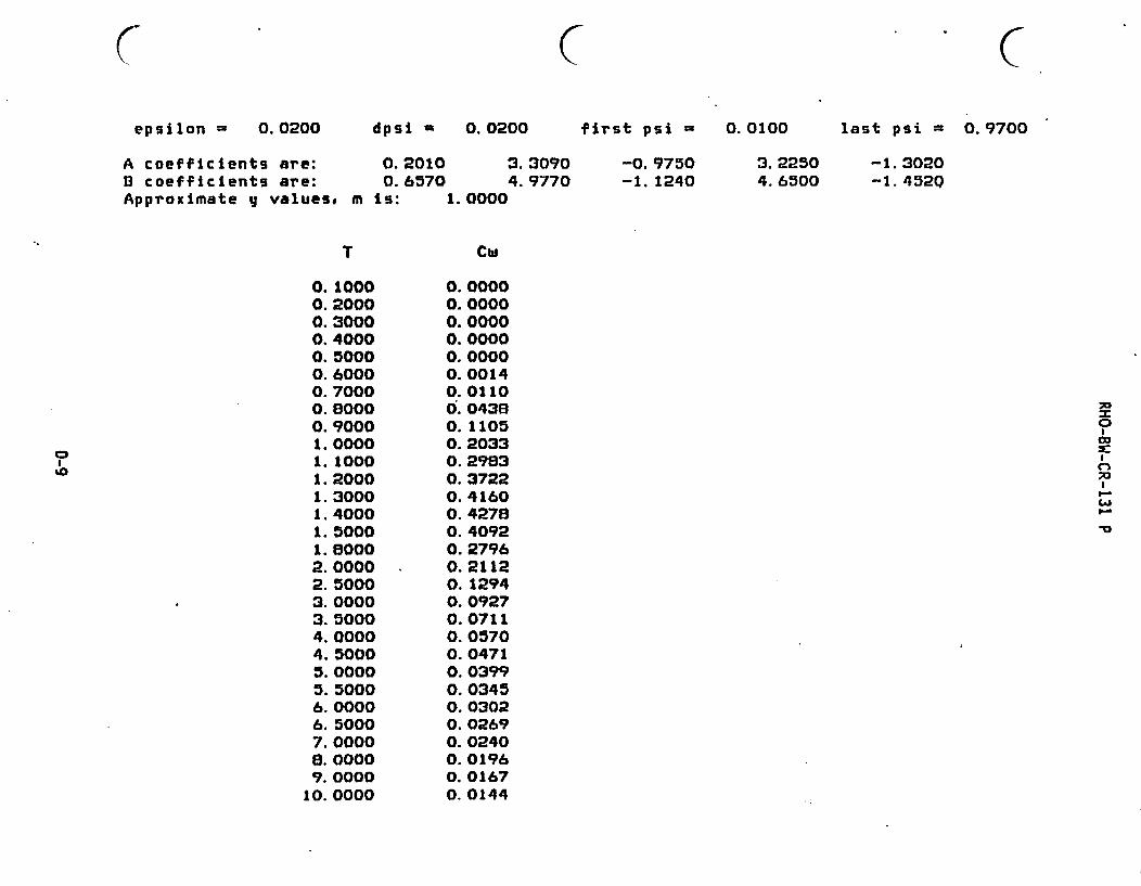
C C cepsilon = 0. 0200 dpsi = 0.0200 first psi = 0. 0100 last psi = 0.9700
A coefficients are:B coefficients are:Approximate y values.
0. 20100. 6570
3. 30904. 9770
-0. 9750-1. 1240
3. 22504. 6500
-1.3020-1. 4520
m is: 1.0000
T Cw
CD
0. 10000.20000. 30000.40000.50000.60000. 70000. 80000. 90001. 00001. 10001. 20001. 30001.40001. 50001. 80002. 00002.50003. 00003.50004. 00004. 5000a. 00005. 50006. 00006. 50007. 00008. 00009. 0000
10. 0000
0. 00000. 00000. 00000. 00000. 00000. 00140. 01100. 04380.11050.20330. 29830. 37220. 41600. 42780.40920. 27960.21120.12940. 09270.07110. 05700. 04710. 03990. 03450. 03020. 02690. 02400. 01980. 01670. 0144

C-
epsilon-
C (0. 0020 dpsi - 0. 0100 f irst psi - 0. 0050 last psi . 0.9750
Exact a valuesExact b valuesExact y values
003
T
0. 10000. 20000. 30000. 40000. 50000. 60000. 70000. 80000. 85000. 90000. 95000. 97501. 00001. 02501. 05001. 07501. 10001. 12501. 15001. 17501. 20001. 22501. 25001. 30001.2001. 40001. 50001. 60001. 60002. 00002. 20002. 5000
0.00000. 00000. 0000O. 00000. 00000. 00000. 0000O. 00030. 00540. 04520. 19440. 32650. 48540. 64640. 78040. 86420. 86710. 65560. 78830. 70650. 62650. 55720. 50070. 41940. 50070. 32440. 26710. 22740. 17500. 14150. 11820. 0941
Cm T
3. 00003. 50004. 00004. 50005. 00005. 50006. 00006. 50007. 00007. 50006. 00009. 0000
10. 0000
Cw
0. 06920. 05400.04380. 03660. 03120. 02710. 02380. 02120. 01900. 01720. 01570. 01330. 0115
0
C,wIi

C C Cepsilon - 0. 0500 dpsi - 0.0200 first psi =
A coefficients are:B coefficients are:Approximate g values,
0. 20100. 6570
m is:
I3. 30904. 9770
1. 0000
0. 0100
3. 22504. 6500
last psi = 0.9700
-1.3020-1.4520
-0. 9750-1. 1240
T Cw
CDI'-a
0. 10000. 20000. 30000.40000. 50000. 60000. 70000. 80000.90001. 00001. 10001. 20001.30001. 40001.50001. 60001. 70001. 80002.00002. 50003. 00003.50004. 00004. 50005. 00005. 50006. 00006. 50007. 00007. 5000S. 00009. 0000
10. 0000
0. 00000. 00000. 00000. 00090. 00770. 02790. 06520.11570.17050. 22140. 26270. 29150. 31020. 32010. 31960. 31010. 29340.27190. 22470. 13640. 09450. 07170. 05730. 04730. 03990. 03450. 03020. 02670. 02390. 02160. 01960. 01650. 0143
'a

C C Cepsilon = 0. 1000 dpsi a 0.0200 first psi = 0.0100 * last psi = 0.9700
A coefficients are: 0.2010B coefficients are: 0.6570Approximate y values. m Is: I
T
3. 30904. 9770
L. 0000
-0.9750-1. 1240
3. 22504. 6500
-1. 3020-1. 4520
Cwe
0
O. 10000.20000. 30000.40000. 50000.60000. 70000.80000. 90001.00001. 10001.20001. 30001. 40001. 50001.60001.70001. 80002. 00002. 50003. 00003. 50004.00004. 50005. 00005.50006. 00006.50007.00007. 50006. 00009. 0000
10. 0000
0. 00000.00000.00210. 01340.03780.07260.11150.14890.18140. 20720.22620. 23860.24720. 25290.25460.25210.24630.23730. 21320.14580. 09980. 07380. 05840. 04760. 04030. 03470. 03030. 02670.02390. 02160. 01960. 01650. 0143

C C. C
epsilon - 0.0200beta = 1. 0000Exact a valuesExact b valuesExact y values
dpsi - 0.0200 f irst psi = 0. 0100 last psi = 0.9700
CD
T0. 10000. 20000. 30000.40000. 50000. 60000. 70000. 60000. 90001. 00001. 10001. 20001. 30001. 40001. 50001. 60002. 00002. 50003. 00003. 50004. 00004. 50005. 00005. 50006. 00006. 50007. 00007. 50006. 00009. 0000
10. 0000
Cw0. 00000. 00000. 00000. 00000. 00060. 01020. 05430. 14750. 26670. 37210. 43760. 45230. 42020. 36280. 30210. 16270. 14410. 09390. 06860. 05340. 04320. 03610. 03060. 02670. 02350. 02090. O16e0. 01700. 01550. 01310.0113

C C Cepsilon = 0.1000
beta = 1.0000Exact a valuesExact b valuesExact y values
dpsi - 0.0200 first psi = 0. 0100 last pSI = 0.9700
'-S
T0. 10000. 20000.30000. 40000. 50000. 60000. 70000.6o0000. 90001.00001. 10001. 20001. 30001. 40001. 50001. 60001. 70001. 60001. 90002. 00002. 50003. 00003. 50004. 00004. 50005. 00005. 50006. 00006. 50007. 00007. 5000a. 0000B. 50009. 0000
10. 0000
Cw0..00000. 00000. 00240.02130.06230.11250. 15930.19710. 22470.24360. 25640. 26360. 26440. 25920. 24870. 23440. 21760. 19960.18150. 16420.10140.07070. .05390. 04330. 03590.03050. 02640. 02320. 02060. 01850. 01670. 01520. 01390. 01280. 0111

( (epsilon = 0.0200
beta = 1.0000Exact a values.Exact b valuesExact y values
dpsi - 0.0100
en
T0. 10000. 20000. 30000. 40000. 50000. 60000. 75000. 80000. 85000. 90000. 95001. 00001. 05001. 10001. 15001. 20001. 25001. 30001. 40001. 50001. 60001. 70001. 50001. 90002. 00002. 50003. 00003. 50004. 00004. 50005. 00005. 50006. 00006. 5000
Cw0. 00000. 00000. 00000. 00000. 00060. 01020. 09540. 14750. 20640. 26670. 32330. 37210.41070.43780. 45180. 45230.44100.42020. 36280. 30210. 25070.21160.18270. 16100.14410. 09390. 06860. 05340. 04330. 03610. 03080. 02670. 02350. 0209
first psi -
T7. 00007. 5000S. 00009. 0000
10. 0000
0. 0050
Cw0. 01880. 01700. 01550. 01310. 0113
last psi = 0.9700

C C cepsilon = 0. 0100 dpsi = 0.0200 first psi = 0.0100 last psi = 0.9700
A coefficients are: 0.2010B coefficients are: 0.6570Approximate yj values# m is: I
T
3.30904. 9770
1. 0000
-0.9750-1. 1240
3. 22504. 6500
-1. 3020-1. 4520
Cw
0
0. 10000.20000.30000. 40000. 50000. 60000. 70000. 60000. 90001. 00001. 10001. 20001. 30001. 40001. 50001. 60002. 00002. 50003.00003. 50004. 00004. 50005. 00005. 50006. 00006. 50007. 00007. 50006. 00009. 0000
10. 0000
0. 00000. 00000. 00000. 00000. 00000. 00000. 00040. 00780. 04690. 14920. 30160.44120. 51710. 51560. 45660. 26400. 20210. 12830. 09240.07110. 05700. 04730. 04000. 03450. 03030. 02690. 02400.02180.01980. 01670. 0144

C' ( Cepsilon = 0.0050 dpsi - 0.0050 first psi - 0. 0025 last psi = 0.9700
A coefficients are: 0.2010B coefficients are: 0.6570Approximate y values. m is:
3. 30904. 9770
1.0000
-0.9750-1. 1240
3. 22504. 6500
-1.3020. -1. 4520
0
T0. 10000.20000. 30000. 40000. 50000. 60000. 70000. 75000.80000. 65000. 90000. 95001. 00001..05001. 10001. 15001. 20001. 25001.30001. 40001. 50001. 60001. 70001. 80001. 90002. 00002. 20002. 50003. 00003. 50004. 00004. 50005. 00005. 5000
Cw0. 00000. 00000. 00000. 00000. 00000. 00000. 00000. 00000.00020. 00160.00780.02710. 07220.15310. 26770. 39790.51590.59940. 63610.56670. 46300.36170.2970
.0.25430. 22330.19910.16350. 12800. 09240. 07120. 05720. 04740. 04020. 0347
T6. 00006. 50007.00006. 00009. 0000
10. 0000
aO
X.
"II--
Cw0. 03040.02700. 02420. 01990. 01680. 0145

( Cepsilon = 0. 0050 dpst - 0. 0100 first psi - 0. 0050 last psi - 0.9750
ExactExactExact
a valuesb valuesV values
a3
T0. 10000. 20000.30000. 40000. 50000. 60000. 70000.80000.90001. 00001. 02501.05001.07501. 10001. 12501. 15001. 17501.20001. 22501. 25001. 30001. 40001. 50001. 60001. 70001. 80002. 00002. 20002. 50003. 00003. 50004. 00004. 50005. 00005. 5000
Cm0. 00000. 00000. 00000. 00000. 00000. 00000. 00050. 01970. 16350. 47220. 54610. 60770. 65320. 67970. 68660. 67580. 6505'0. 61530. 57430.53160. 45140. 33770. 27220. 22970. 19900. 17550.14150.11810. 09390. 06890. 05380. 04360. 03640.03110. 0270
T6. 00006. 50007. 00008. 00009. 0000
10.0000
:0CDwI
LAI
I-I
Cw0. 02370.02110. 01900. 01570. 01320.0114

RHO-BW-CR-131 P
APPENDIX E
SCIENCE APPLICATIONS, INC. TRACER TEST DATA IN BOREHOLES DC-7/8(reproduced from a report submitted by
K.I<_ Science Applications, Inc.)
K>
E-1

RHO-BW-CR-131 P
APPENDIX E
TRACER TEST IN BOREHOLES OC-7/8
The tracer test* was conducted as follows:
* With the shut-in tool open in both holes, pumping out of DC-7 wasstarted and continued for 2 days (before injecting the tracer mate-rial) at a discharge rate of ap2yt 1.3 gal/min. Approximately47.0 mCi of the water-soluble I tracer material were frozenusing dry ice. The frozen isotope was dropped (two small uncoveredplastic vials) into DC-8. Between 30% to 60% of the total dischargevolume out of DC-7 was injected into DC-8 until arrival of thetracer material at DC-7 is detected. The remaining water wasdiverted to a nearby pit.
* Following detection of the arrival of 131I at the pumping well,all water coming out of DC-7 was injected or recirculated intoDC-8. Triangle Service Company placed a 1 3/8-in.-outside-diametergamma detector tool at the wellhead of DC-7, and monitoring on a24-hr basis was conducted by Triangle personnel. This procedurehelped avoid contaminating tools, wireline, or other related equip-ment by radioactive material. Figure E-1 shows the surface equip-ment setup used in the tracer test. Pressure response in the twoholes was monitored continuously since the interval was straddledNovember 29, 1979 until the end of testing December 14, 1979.
TESTS, DC-7 AND 8/IF/9/TTO0
Data for the test are presented in Tables E-1 through E-4.
Figure E-2 shows part of the record obtained from the tracer experiment:Part A represents the background level; Parts B and C show the beginning andthe end, respectively, of the continuous rise of activity at the DC-7 welihead;Part D shows the steady flow of activity.
The activity (counts/inch) versus time in hours is shown in Figure E-3.Another graph is obtained from it by plotting the activity versus elapsedtime since injection as shown in Figure E-4. The tracer material was detectedat the OC-7 wellhead after 8 hr following its injection at DC-8. Theactivity increased sharply and peaked within <1 hr after it was firstdetected.
*The test yielded a value of 2.5 x 10⁻² ft2/s for the product nb, whereb = 49.8 ft. The dispersivity obtained from the test is 1.1 ft.
E-2

C 'C
DETECTION EQUIPMENT NOT 70 SCALE
~METER
1. DETECTOR a
10Sf 1 9o5 | s <8.4 ft
- 249 f PIEZOMETRIC SURFACE - -- x -
01~~~~~~~~~~~~~~
5 in. 298.5 ft 1.6 in.
- ~~~~~~~~~3.03 In--.PUMP2.87 In. f
1 ~~~~~~~~46.2 ft
2.44 in. PACKERS
8.66 s | / 49.8 ft PERMEABLE ZONE
DC-7 DC-B
FIGURE E-1. Schematic of Tracer Test Setup.'.

RHO-BW-CR-131 P
TABLE E-1. Site Log for Test DC-7 and 8/IF/z9/TTOlTracer Test.
S - S 5-
STATUS ACTIVITY TIME DATE BY
PREPARE FOR TRACER TEST 12:01 12/08/79 KGK
DC-7 POMP ON 12:09 12/08/79 JB
START TRACER TEST DC-7&8/IF/9/TTO1 15:00 12/11/79 AAB
DC-8 DROP TWO FROZEN VIALS CONTAININGRADIOACTIVE MATERIAL (IODINE-131) 15:05 12/11/79 WS
DC-8 CIRCULATE: PART OF THE WATER PUMPED 15:16 12/11/79 WSOUT OF DC-7 IS INJECTED INTO DC-8
DC-7 TRACER MATERIAL SHOWING UP IN THE 22:57 12/11/79 AH* ~~PUMPED WATER225 12179 A
DC-7 CIRCULATE (INJECT) ALL WATER PUMPED 23:05 12/11/79 AHOUT OF DC-7 INTO DC-B
DC-7 STOP MONITORING OF RADIOACTIVEMATERIAL; REMOVED DETECTING EQUIPMENT 18:50 12/12/79 MB
END TRACER TEST DC-7&D/IF/9/TTO1 PUMP OFF 13:59 12/13/79 AABIN DC-7
E-4

RHO-BW-CR-131 P
TABLE E-2. Raw Data For Test DC-7/IF/z9/TtOl.(Sheet I of 9)
RAW DATA FROM 12. I 12: 92 0 TO 12.13 142 02 0
YYODOSSSSS DATE TIME INDEX POES Ps
793424374079342437657934243790793424301579342436407934243165"734243890793424391579342439407934243945934243990
79342440157934244040793424406579342440917934244116793424414179342441667934244191734244216734244241793424426479342442927934244316793424434179342443667934244391793424441679342444417934244466793424449279342445277934244567n9342445927934244417
12.12.12.1:.12.12.12.12.12.12.12.12.12.t2.12.12.12.12.1.12.
12.12.12.t2.12.12.12.12.12.12912.12.12.12.12.
a 221 92 0* 121 9:25* 121 9:SO* 12210115* 12t10:40* 12211t 5* 12:11:30* 122llt551 t2t21220* 1211224S* 12213110* 12113235* 121141 08 122141253 12t141SZ* 12215t16* 12:15241e 12116: 6
* 123 16:31I 12114:56* 12217221* 12:12S34
1 1216219:1I 12219:23
* 12:19:26* 12:G19t2U 122202268 IM1t15* 12:22014
8 12123123
I 12123137
123456709tl11121314is1617
1920212223:4
27
2829303132333435
0 .0000.0000.0000.0000.0000.0000.0000.0000.0000-0000.0000.0000.0000.0000.0000.0000.0000.0000.0000.0000.0000.0000.0000.0000.0000-0000.0000.0000.0000.0000.0000*0000.0000.0000.000
PRCS P2
1423.8721423.0411423.2901421.7371420.9031420.2141419 .6081419*.060t141.5551413.3091416.0491417.7461417. 4831427.2.81416.93114146.8291416 5401416.2351415.9361415.4091415.1101414.9131414.6771414 5941414 3531414.2401414.0401413.9341413.1371413.6711413. 5141413.4131413. 0901413.0211412.383
PRE$ PS
0.0000.0000.0000.0000.0000.0000.0000.*0000.0000.0000.0000.0000.0000.*0000.0000.0000.0000.0000.000o *0000.0000.0000.0000.0000.0000.*0000.*0000.0000.0000.0000.0000.000'0.*0000.0000.000
RAW DATA FRON 12. U 122 90 O TO 12.13 141 Of 0
VYDODSSISS DATE TIME INDEX PRES Pt PRES P2 PRES P3
793424464279342446677934244692734244717n9342447427934244767793424479279342446177934244842793424486779342448937934244916n934244943n9342449667934244993934243013
7934245043n9342450667934245093793424511679342451437934245169793424519379342452187934245:4379342452637934245294793424331979342453447934245369793424Z394793424542979342454447934245469793424Z494
12.12.12.12.12.12.12.12.12.12.12012.12.12.12.12.12212.12.12.12.12.12.12.22.12.12.12.12.12.12.12.12.12.22.
12224: 212124:2712*24:52
1t21221712:25242121261 71212613212:2625712227:22122272471212311312212833121292 312:22:9212229253
1213011312230:43122312 612:31233122231 2581213212312232246G1213311312:33:38122342 312:34: 212234 254121352191223524412U36 91223623412136259121 37124122372 4912232:14
363733394041424344454647484950S1525354555657565960616263646566676*
6970
0.0000.0000.0000.0000.0000.0000.0000.0000.0000.0000.0000.0000.0000.0000.0000.0000.0000*0000.0000.00000000*0000.0000.0000.0000.0000.0000.0000*0000.0000.0000.0000.0000.0000.000
1412.7581412.6591412.5141412.3891412.2461412.2161412.0571411.9791411.9171411.6361411.7341411.6541411.5571411.4921411. 3721411.3291411.2:8t411. 1001410.996410.9131410.3581410.7311410 .381410.5391410.5691410.4461410.3701410. 2981410.2191410.1651410.0981409.9251409 .8871409.7621409.&G5
0.0000.0000.0000.0000.0000.0000.0000.0000.0000 0000.0000.0000.0000.0000.0000.0000.0000.0000.0000.0000.0000.0000.0000.0000 .0000.0000.0000.0000.0000.0000.0000.0000.0000.0000.000
E-5

RHO-BW-CR-131 P
TABLE E-2. Raw Data For Test DC-7/IF/z9/TtOl.(Sheet 2 of 9)
RAW DATA FROM 12. S 12t 9* 0
YTDDDSUSSI DATE 1TME
To 12.13 14t l 0a
INDEX PRS pS PRS P2 PRES P3
7934245S57934245995793424619679342463967934246597793424679779342469987934247193793424739979342475997934247800793424055179342491537934249754"34250356793425095779342542411793425301379342536147934254216793425481779342=541979342S60207934256621793425722379342573247934258426"342590277934259629793424023079342609317934261433793424203479342626367934263237
12.12.12.12.12.12.12.12.12.12.12.12.12.12.12.12.12.12.12.12.12.12.12.12.12.12.2.12.12.12.12.12.12.12.12.
1214321512146*35121491561215311612156:3712159s57131 3218131 6130131 9159131.1311931316140131291 1113239123t384V11413159:4t141 9:1714333:3114143:3314 53:341s5 3:3615113:3715123: 3S25t33:43
143:4115253:43
161 3:4416123:&716:33:&916S43:1
172 3153
17113:!.'
17: T:%3
17123:Z617133:T7
71727374'576777.SI
soat6263.4
6760
9091929394989'979.V9
100101102103104105
0.0000.0000.0000.0000.0000.0000.0000.0000O0000.0000.0000.0000.0000.0000.0000.0000.0000.0000.0000*0000.0000.0000.0000.0000.0000.0000.0000.0000.0000.0000.0000.0000.0000.0000.000
1409.727140E.2091407.6331406.9641406.4721405.9201405.9821406.2441407 2491407 3941407.3771406.e731406.1761405.5451404.3051404.1491402.5531402.0291401.3211400.1092400.2441399.7131399.152139. 7111399.2301397.8S51397.3531396.8941396.4301395.999t395.5931395.2291394.6151394.4611394.052
0.0000.0000.0000.0000.0000.0000.0000.*0000 * 000
0.0000.0000.0000.0000.0000.0000.*0000.*0000.0000.0000.0000.0000.*0000.0000.0000.0000.0000.0000.*0000.0000.*0000.0000.0000.0000.0000.000
0.000
RAW DATA FROM 12. 6 12 91 0 TO 12.13 141 os 0
YTDDDSSSSS DATE MINE INDEX PRES PI PRES r2 PRES P3
793426383879342644407934265041.734265643734266244934266945
79342674477934269046793426965073426925179342698537342704547934271055793427165779342722S9734272860
9342734617342740627934274664793427526!7934275677342764637934277069793427767179342732727934278974n93427947579342600767934360678793429127979342819187934262492793429309379342036957934264226
12.12.12*
12.12.12.12.12.12.12.12.12.12.12.12.12.12.12.12.12.12.12.12.12.12.12.12.12.12.12.12.12.12.12.
e 171431580 171541 0e 162 41 1a 16214S 3* 181241 43 131341 56 163441 7* 131541 UU 191 4110a 19114111a 191241139.19134114* 191441156 191541176 201 4S11a 201142208 20124121* 201341226 201441246 201541256 212 42276 21814128* 211241298 21334331* 211441326 21254134* 221 4135* 22114136* 221241336 221341396 228442418 22254142e 23S 41438 23114145* 23224146
106107too109lot
110III
11211311411511611711e119120121122123124125126127128129130131132133134135136137138139140
0.0000.0000.0000.0000.0000.0000.0000.0000.0000.0000.0000.0000.0000.0000.0000.0000.0000.0000.0000.0000.0000.0000.0000.0000.0000.0000.0000.0000.0000.0000.0000.0000.0000.0000.000
1393.7923393.4891393.0951392.3211392.5031392.1381391.9061391*6611391.3201391.0981390.6601390.6671390.3491390.1511389.9571389 72B138994381389 3321389.0721398.9061388.6961388.5821388.4051388.1351387.9941387.1051307.7671387.589I987.4201397.2801397.0301306.8451386.7281386.5361386.449
0.0000.0000.0000.0000.0000.0000.0000.0000.0000.0000.0000.0000.0000 .0000.0000.0000.0000.0000*0000.0000.0000.0000.0000.0000.0000.0000.0000.0000.0000.0000.0000.0000. 0000.0000.000
E-6

RHO-BW-CR-131 P
TABLE E-2. Raw Data For Test DC-7/IF/z9/TtOl.(Sheet 3 of 9)
RW DATA FROM 12. I 12S 92 0 TO 12-13 148 os 0
VYDDDSSZS5 DATE TIME INDEX PRES Pt PRES P2 PRES P3
7934248997 12. 23234147 141 0.000 1386.302 0.0007934205499 12. e 23144:41 142 0.000 1386.104 0-0007934296090 12. e 23254:50 143 0.000 1386.035 0.0007934300292 12. 9 02 4:52 144 0.000 1385-905 0.0007934300993 12. 9 014:53 145 0.000 1385.72? 0.000n934301494 12. 9 022454 146 0.000 1385.647 0-0007934302096 12. 0234256 147 0.000 1305.544 0-0007934302697 12* 0244257 148 0.000 1385.374 0.000793430329t 12.* 9025459 149 0.000 1385.306 0.0007934303900 12. 9 8 5S 0 150 0.000 13853.165 0.0007934304501 12. 9 1213 I 151 0.000 1385.043 0.0007934305103 12. 9 1225 3 152 0.000 1384.944 0.0007934305704 12* 911352 4 153 0.000 1334.579 0.0007934306306 12. 9* 1458 154 0.000 1384.722 0.0007934306907 12. 91* 55* 7 155 0.000 1384.653 0.0007934307`500 12. 9 22 5S 156 0.000 1384.542 0.0007934309110 12. 2215210 157 0.000 1384.475 0.0007934309711 12. 9 225111 159 0.000 1304.375 0000o7934309312 12. 9 21351,2 159 0.000 1304.263 0.0007934309914 12. 2245:14 160 0.000 1384.153 0.080793431015 12. 9 2155:15 161 0.000 1384.119 0.0007934311117 12. f32 5117 162 0.000 1384*024 0.000793431721 12. 93 311511 163 0.000 1383.979 0.0007934312319 12. 93 25219 164 0.000 1383.143 0.0007934312921 12. 9 335121 165 0.000 1303-.16 0.0007934313S22 12. 9 3145:22 164 0.000 1385.077 0.0007934314124 12. 9 3155124 167 0.000 1395.449 0.0007934314725 12. 9 41 S25 168 0.000 1385.642 0.0007934315326 12. 9 M 481512 169 0.000 1395.11 0.0007934315923 12. 9 4225229 10 0.000 1386.109 0.000793431629 12. 9 4135129 171 0.000 1386.211 0.0007934317131 12. 9 4845231 172 0.000 1386.470 0.0007934317732 12. 9 4855832 173 0.000 1386.652 0.0007934311333 12. 9 5 333 174. 0.000 1386.797 0.0007934311935 12. 9 515135 17n 0.000 1386.t0 0.000
RAW DATA FROM 12. 121 92 0 TO 12.13 141 02 0
YYDDDSSSSS DATE TIME INDEX PRES Pt PRES P2 PRES Ps
7934319536 12. 9 52t36 176 0.000 1337.116 0.0007934320137 12. 9 5235237 177 0.000 1387.364 0.0007934320739 12. 9 534539 179 0.000 1387.476 0.0007934321340 12. 9 53SS140 t79 0.000 1387.712 0.0007934321942 12. 9 68 5842 tSo 0.000 1387.735 0.0007934322543 12. 9 6215843 lot 0.000 1387.905 0.0007934323144 12. 94 12544 182 0.000 1388.07 0.0007934323746 12. 9 6235246 13 0.000 1388.205 0.0007934324347 12. 9 624547 194 0.000 13889.32 0.0007934324949 12. 9 6255249 185 0.000 1399.395 0.000793432550 12. 9 71 5250 196 0.000 1398.471 0.0007934326151 12. 9 721551 157 0.000 1389.622 0.0007934326753 12. 9 7125253 lee 0.000 1398.675 0.0007934327354 12. 97 735154 to 0.000 1388-.45 0.0007934327956 12. 9 724556 19o 0.000 1388.931 0.0007934329557 12. 9 7255157 191 0.000 1388.974 0.000934329158 12. 9 3 5258 t92 0.000 1389.097 0.0007934329760 12. 9 2162 0 1ts 0.000 1389.151 0.0007934330361 12. 9 2262 1 194 0.000 1389.252 0.000793433O963 12. 9 5236 3 195 0.000 1389.339 0.0007934331564 1 9l2 924: 4 196 0.000 1399.334 0.0007934332165 12. 9 5156 5 197 0.000 138T.443 0.0007934332767 12. 991 61 7 199 0.000 1399.S39 0.0007934333369 12. 9 92162 a 19* 0.000 1389.745 0.0007934333970 12. 9 9224310 200 0.000 1399.676 0.0007934334571 12. 9 913621 201 0.000 1389.641 0.0007934335172 12. 9 9t4612 202 0.000 1398.656 0.0007934335774 12. 9 9256214 203 0.000 1338.644 0.000934336375 t2. 9t10 6115 204 0.000 1389.676 0.0007934336977 12. 9 1031617 205 0.000 1399.631 0.0007934337579 12. 9 1012619 206 0.000 1399.676 0.0007934338179 12. 9 1023619 207 0.000 1399.717 0.0007934338791 12. 9 1024621 203 0.000 1389.723 0.0007934339382 12. 9 1056:22 209 0.000 1389.676 0.0007934339994 12. 9 11 6324 210 0.000 1339.710 0.000
E-7

RHO-BW-CR-131 P
TABLE E-2. Raw Data For Test DC-7/IF/z9/TtOl.(Sheet 4 of 9)
RAU DATA FROM 12. I tIt *s o 012.13 141 0 0
YYcDDSSSSs DATE TIRE INDEX PRES FP PRES U2 PRE$ F3
7934340565 12. 9 11116275 211 0.000 1399.699 0.0007934341186 12. 9 1112t22 212 0.000 1389.693 0.0007934341788 12. 9 11136120 213 0.000 1399.631 0.0007934342389 12. 9 11146229 214 0.000 1389.611 0.0007934342991 12. 9 11156131 21S 0.000 1389.760 0.0007934343592 12* 9 12: 6832 216 0.000 1389.792 0.0007934344193 82* 9 12116333 217 0.000 1399.7e4 0.00079343447n5 12. 9 12126835 216 0.000 139.s738 0.0007934345396 12. 9 12136136 219 0.000 1389.829 0.000793434s99s 12 * 12246838 220 0.000 1389. 39 0.0007934346599 12. 9 12256139 221 0.000 1389.792 0.0007934347201 12. 9 133 6241 222 0.000 1399.794 0.0007934347902 12. 9 13316t42 223 0.000 1389.343 0.000n934348403 12. 9 13226343 224 0.000 1389.794 0.0007934349005 12. 9 13836:45 225 0.000 1389.770 0.0007934349606 12. 9 13:41:46 226 0.000 1389.924 0.0007934350206 12. 9 13156148 227 0.000 1389.139 0.0007934350909 12. 9 141 6149 229 0.000 1389.787 0.0007934351410 12. 9 1411:650 229 0.000 1389.831 0.0007934352012 12. 9 14322:52 230 0.000 1389.849 0.0007934352613 12. 9 14136353 231 0.000 1399.804 0.0007934353215 12. 9 14146155 232 0.000 1399.704 0.0007934353381 12. 9 14256156 233 0.000 1389.811 0.0007934354417 12. 9 151 6157 234 0.000 13899849 0.0007934356749 12. 9 15145149 235 0.000 1399.775 0.0007934359552 12. 9 16115152 226 0.000 1399.821 0.0007934360356 12. 9 16145156 237 0.000 1389.729 0.0007934362160 12. 9 172163 0 228 0.000 1399.470 0.0007934363965 12. 9 171462 5 239 0.000 1399.676 0.0007934365769 12. 9 161161 9 240 0.000 1389.713 0.0007934367573 12. 9 11246813 241 0.000 1389.636 0.0007934369377 12. 9 19116117 242 0.000 1399.651 0.00o7934371131 12. 9 19246221 243 0.000 1389.623 0.0007934372986 12. 9 20116t26 244 0.000 1389.641 0.0007934374790 12. 9 20146130 245 0.000 1399.562 0.000
RAW DATA VROM 12.. 3 121 91 0 TO 12.13 142 o0 0
TTDDDSSSSC DATE TIME INDEX FRES PI F RES P2 PRES P3
7934376594 12. 9 21116:34 246 0.000 1389.5Z2 0.0007934378393 12. T 21U46:38 247 0.000 1389.603 0.0007934390202 12. 9 22216142 248 0.000 1389.542 0.0007934382007 12. 9 22246147 249 0.000 1389.587 0.0007934393911 12. 9 23116151 250 0.000 1399.641 0.0007934395615 12. 9 23146155 251 0.000 1389.612 0.0007934401019 12.s0 011159 252 0.000 1389.673 0.0007934402923 12.10 0147t 3 253 0.000 139*611 0.0007934404623 12.10 12172 8 254 0.000 1389.653 0.0007934406432 12.10 1847212 255 0.000 1389.656 0.0007934408236 12.10 2817816 256 0.000 1389.700 0.0007934410040 12*10 2147120 257 0.000 1389.653 0.0007934431644 12.10 3117124 2-8 0.000 13899.68 0.0007934413649 12.10 147129 259 0.000 1389.604 0.000n934415453 12.10 4117:33 260 0.000 1389.614 0.0007934411460 12.10 5S 7240 261 0.000 1389.591 0.0007934420264 12.10 5t37144 262 0.000 1389-916 0.000734422068 12.10 61 7249 263 0.000 1399.572 0.0007934423872 12.10 6137252 264 0.000 1389.636 0.0007934425677 12.10 72 7257 265 0.000 1389.572 0.0007934427481 12.10 71382 1 266 0.000 1389.547 0.0007934429285 12.10 11 38 5 267 0.000 1399.445 0.000"3443108T 122.0 51388 9 268 0.000 1399.493 0.0007934432894 12.10 91 8214 269 0.000 1399.471 0.000793443469e 12.10 9239312 270 0.000 1389.599 0.0007934436502 12.10 101 8922 271 0.000 1389.309 0.0007934438306 12.10 10139:26 272 0.000 2369.951 0.000t934440110 12.10 IS: 6330 273 o.000 1389.755 0.0007934441915 12.10 1138135 274 0.000 1389.599 0.0007934443719 12.10 122 6239 275 0.000 1380.47n 0.0007934445523 12.10 12239843 276 0.000 1376.506 0.0007934447327 12*10 131 3t47 277 0.000 1380.400 0.0007934449131 12.10 13238951 279 0.000 1381.135 0.0007934450935 12.10 143 ss55 279 0.000 1391.552 0.0007934452739 12.10 14383159 290 0.000 1381.839 0.000
E-8

RHO-BW-CR-131 P
TABLE E-2. Raw Data For Test DC-7/IF/z9/TtOl.(Sheet 5 of 9)
RA DATA FRO" 1:2. 9 12S 91 0 tO 12.13 141 o0 0
YDDDSSSSS DATE Timt INDEX PRES Ft PRES P2 URES P3
7934455030 12.10 15317110 211 0.000 1382.099 0.0007934454834 12.10 15147214 212 0.000 1382.684 0.0007934450438 12.10 16317211 293 0.000 1384.S64 0.0007934460442 12.10 16t47t22 214 0.000 138J5.54 0.0007934462244 £2.10 17111724 295 0.000 1383.613 .00007934464051 12st0 17247231 294 0.000 13985495 0.0007934465985 12.10 11217235 297 0.000 1385.944 0.000734467659 12.10 18247239 208 0.000 1396.326 0.000.n34469463 12.10 19217143 299 0.000 1384.715 0.000n934471267 12.10 19247147 290 0.000 1387.037 0.000n934473071 12.10 20M17151 291 0.000 1387.308 0.0007934474876 12.10 20247156 292 0.000 1387.626 0.0007934474680 12.10 212112 0 293 o0.000 1387.01 0.0007934476494 12.10 212411 4 294 0-000 1387.990 0.0007934480298 12.10 22:192 6 295 0.000 1388.250 0.0007934482092 12.t0 22248212 294 0.000 1388.422 0.0007934489897 12.10 23213217 297 0.000 1398.544 0.000934486701 12.t0 23249221 298 0.000 1388.720 0.000793450205 12.11 0218225 299 0.000 1388.93 0.000n934502909 12lI1 0248229 300 0.000 1388.950 0.0007934504713 12.11 1219133 301 0.000 1319.096 0.0007934506511 12.11 1248t39 302 0.000 1389.191 0.0007934508322 12.11 2219242 303 0.000 1389.257 0.0007934510132 12.11 2248t46 304 0.000 1389.408 0.000n934511930 12.11 32192SO 305 0.000 1389.525 0.0007934513734 12.1 3 2:4854 304 0.000 1389.439 0.000793455393? 12.1t 411S959 307 0.000 1389.703 0.0007934517343 12.12 42492 3 309 0.000 198.9756 0.0007344519147 12.11 519 7 309 0.000 1389.767 0.0007934520951 12.11 5249U11 310 0.000 1389.092 0.0oo7934522755 12.11 6119215 311 0.000 1389.922 0.0007934524540 12.11 6249T20 312 0.000 1391.098 0.0007934526364 12.11 7219124 313 0.000 3839.690 0.0007934529722 12.11 3115222 314 0.000 1384.134 0.0007934532027 12.11 81S1347 315 0.000 1387.259 0.ooo
ItM DATA FROM 12. 9 12* 91 0 TO 12.13 24* os 0
vYvDZSSSSS DATE TIIt INDEX PotS PI PRES P2 MtEg r3
7934532153 12.11 9255S13 316 0.000 1397.304 0.0007934532276 12.*11 *15758 317 0.000 1387.330 0.0007934532403 12.11 91 O0 3 319 0.000 '1397.36 0.0007934532529 12.11 92 229 319 0.000 1387.353 0.0007934532654 12.11 91 4t14 320 0.000 1387.404 0.0007934532779 12.11 91 6119 321 0.000 1387.419 0.0007934532904 12.11 91 9224 322 0.000 1387.411 0.0007934333030 12.11 9210230 323 0.000 1387.453 0.0007934533155 12.11 9S12135 324 0.000 1387.491 0.0007934534496 12.11 93216 325 0.000 1387.670 0.000793453599 12.11 9253319 324 0*000 1387.818 0.0007934536501 12.11 102 9221 327 0.000 1387.8?2 0.0007934537403 12.11 10223223 329 0.000 1387.995 0.000n934539305 12.11 10283125 329 0.000 1389.076 0.0007934539207 12.11 10253:27 330 0.000 1389.222 0.oo0"734540109 12.11 112 8229 331 0.000 1388.331 0.000n934541011 12.11 11223231 332 0.000 1388.399 0.000793441913 12.11 11238233 333 0.0oo 138*490 0.0007934542915 12.11 11253235 334 0.000 13898.75 0.0007934543717 12.11 122 6*37 335 0.000 1388.s71 0.0007934544620 12.1S 12223240 336 0-000 1388.724 0.0007934545522 12.11 12238142 337 0.000 1388.754 0.0007934544424 12.11 12:53*44 338 0.000 1398.913 0.6007934547326 12.11 132 9246 339 0.000 13889.17 0.000n34549229 12.11 13323248 340 0.000 1389.099 0.0007934549857 12.11 13250257 341 0.000 1389.971 0.0007934550759 12.11 142 5259 342 0.000 1389.028 0.0007934551661 12*11 142212 1 343 0.000 1389.060 0.0007934556243 12.11 142362 3 344 0.000 1389.099 0.0007934553390 12.11 14249250 345 0.000 1389.058 0.0007934553415 12.11 14:50ts 346 0.000 1389.070 0.0007934553440 12.11 14250840 347 0.000 138t.141 0.0007934553465 12.11 14251t 5 348 0.000 1389.142 0.0007934553490 12.11 14:51130 349 0.000 1389.100 0.0007934553515 12.11 14251255 350 0.000 1389.134 0.000
E-9

RHO-BW-CR-131 P
TABLE E-2. Raw Data For Test DC-7/[F/z9/TtOl.(Sheet 6 of 9)
RAW DATA FROM 12. 8 12: 91 0 TO 12.13 14S 0 0
YTDDDSSSSS DATE TIME INDEX PRES Pi FRES P2 PRES P3
79345535407934553565793455359079345536157934553641793455366679345536917934553716793455374179345537447934553791793455381479345538417134553866793455389179345539167934553941793455396679345539917934554016793455404179345540677934554092793455411779345541427934SS416779345541927934554217793455424279345542677934554292793455431779345434279345543677934554392
12.1112.1132.1112.1112.1212.1122.1112.1112.1112.1112.1112.1112.1112.1112.1t12.1112.1112.1112.1112.1112.1112.1112.1112.1112.1112.1112.1112.1112.1112.1112.1112.1112.1112.1112.11
14152t2014252:45£41531101415313514*t4t 1143541261415415114S55S16141552411415Ut 6141562311415615614S572211425724614 :58111458136142591 114:59:261425951153 0316151 014115* is 7152 113215t 1157151 2:22152 224715t 3S121S2 3237151 4t 215S 4327151 415215t 5817151 5242515 6t 7
151t 132
351352.35335435535'357358359360261362363364365366367361369370371372373374375376377378379380381382383384385
0o0000.0000.0000.0000.0000.0000.0000.0000.0000.0000.000O.0000.0000.0000.0000.0000 .0000.0000.0000.0000-0000.0000.0000.0000.0000.0000.0000.0000.0000.0000.0000.0000.0000.0000.000
1389 1761389.16113E8 9t21388 059t387. 3441386.84&1386 317S385.3881385.4331305.068134. 7371384.4221384.1031383.8521383.5721383.2961383.1121382.1321382.6471382.4771382.3271382.1571381.9861381.7591381.62213S1.4221381.2571381.0941380.961S380.0211380.7241380.5651380.45813E0.3492380.237
0.0000.0000.0000 * 0000.0000.0000.0000.0000.0000 * 0000.0000.0000.0000.0000.0000.0000.0000.0000.0000.0000.0000 .0000 * 0000.0000.0000.0000.0000.0000.0000.000O * 0000.0000.0000.0000.000
RAM DATA FROM 12. 8221 92 0 TO 12.13 141 01 0
YYDDDSSSSS DATE TIME INDEX FRE£ P1 PREE P2 PREU P3
79345544177934S544427,345544'77934554493793455451179345545437934554368793455459379345546187934554643793455469379345547117934554743n9345547687934S54n7934554816n34554843793455486979345548937345549167"34554,43793455496979345549947934555019n934555044n93453506979345550947934555ll979345551447934555169n9345551947934555219n93455524479345552697934555294
12.1112.1112.1112.1112.1112.1112.1112.1112.2112.1112*1112.1112.1112.1112.1112.1112.81'12.1112.1112.11t2.1t12ll12.1112.1112.1112.1112.2112*.1
12.1112.1112.1112.1112.11
12.1112.11
151 62571SS 7t22152 7t4715S 813315s 323915S 92 3152 9122152 91531510 1151521014315U11331211253815112123151121481511311315S13138152142 315214s22is514153152s1s181511514315316t 915116234t5tl259151171241511714915118214slE5:39i5t29 4
151191291511915425220191522014415*21t 915:21134
386so?387389390
3923933943953963,739,399400401402403404405406407408409410411412413414415416417418419420
0.0000.0000.0000.0000.0000.0000.0000.0000.0000.0000.0000.0000.0000.0000*0000.0000.0000.0000.0000.0000.0000.0000.0000.0000.0000.0000.0000.0000.0000.0000.0000.0000*0000.0000.000
1380.1601380 .0471379.9131379 .511379.7471379.6461379 5441379.4111379 3271379.2381379.0731371.9911379.9311378 101378.8421373.8341378.7441378.7531379.7601378.6781378.5651378.5641379 .0931379.4851379.9491380.4002380.6251380.9011381. 1751381.4471381.4791381 5161381.4771381.4641381.479
0.0000.0000.0000.0000.0000.0000-00000000.0000.0000.0000.0000.0000.0000.0000.0000.0000.0000.0000.0000.0000.0000.0000.0000*0000.0000.0000.0000.0000.0000.0000.0000.0000.0000.000
E- 10

RHO-BW-CR-131 P
TABLE E-2. Raw Oata For Test DC-7/IF/z9/TtOl.(Sheet 7 of 9)
RA^ DATA FROM 12. 8 122 98 0 TO 1213 14t 0S 0
7YDDDSSSSS DATE TIME INDEX PRE$ Pi PRES P2 PREg P3
7934555319 12.11 51321259 421 0.000 1381.439 0.0007934555344 12.21 11522:24 422 0.000 1391.444 0.0007934555369 12.11 15122249 423 0.000 1301.455 0.0007934s5539S 12.11 15:2315S 424 0.000 1301.454 0.0007934555420 12.11 15223240 425 0.000 1301.454 0.0007934s55445 12.11 15:243 5 426 0.000 1391.448 0.0007934555470 12.11 15324830 427 0.000 1391.37 0 .0007934555495 12.11 15224255 420 0.000 13981.35 0.0007934555520 12.11 15225:20 429 0.000 1381.361 0.0007934555545 12.11 15225245 430 0.000 1381.377 0.0007934555570 12.11 M522UMo 431 0.000 1301.412 * 0.0007934555595 12.11 15:26135 432 0.000 1331.354 0.0007934555620 12.11 151271 0 433 0.000 1381 .317 0.000n934555645 12.11 25:27225 434 0.000 1381.294 0.0007934555670 12.11 15827150 435 0.000 1391.27 0.000734555695 12.11 15821215 436 0.000 1301.302 0.0007934555720 12.11 I521140 437 0.000 13o1.338 0.00079345s5745 12.11 151291 5 439 0.000 1381.310 0.0007934555770 12.11 15229t30 439 0.000 1391.296 0.000934555795 12.11 15:29t35 440 0.000 13.81254 0.000
7934555s20 12.11 15230120 441 0.000 1391.271 0.0007934555946 12.11 158301t4 442 0.000 1381.294 0.0007934556246 12.11 15237126 443 0.000 1380.946 0.0007934556547 12.12 15142127 444 0.000 1380.742 0.0007934556040 12.11 15:47128 445 0.000 1380.517 0.0007934557975 12.21 168 4135 446 0.000 1379.668 0.0007934559477 12.11 16214237 447 0.000 1382.459 0.0007934559070 12.21 16224239 448 0.000 1382.434 0.0007934559679 12.11 16234139 449 0.000 1334*175 0.0007934560291 12.11 16t44141 450 0.000 1383.570 0.0007934560082 12211 16354242 451 0.000 1384.054 0.0007934561493 12.11 17t 4143 452 0.000 13984.31 0.0007934562085 22.11 17:14t45 453 0.000 1384.640 0.0007934562696 12*11 27224846 454 0.000 1384.974 0.0007934563289 12.11 t7:34:48 455 0.000 1385.222 0.000
RAW DATA FROM 12. 9 2t 98 0 TO 12.13 141 o0 0
YTDDDSSSSS DATE TIME INDEX PRtU Pi PRES P2 PRE$ P3
7934563889 122.1 17844149 456 0.000 1385.477 0.0007934564490 12.tl 27254850 457 0.000 1395.764 0.00079345 6092 12.1i 198 4252 458 0.000 1385.974 0.0007934565693 12.21 19214853 459 0.000 1386.135 0.0007934566295 12*11 19:24855 460 0.000 1396.399 0.0007934566996 12.11 10834856 461 0.000 1396.567 0.0007934567497 12.11 81944257 462 0.000 1386.760 0.000934569099 12.11 19154859 463 0.000 1386.942 0.000
7934569700 12.11 192 St 0 464 0.000 3837.123 0.0007934569302 12*11 192152 2 465 0.000 1387.322 0.000"734569903 12.11 198252 466 0.000 1387.499 0.0007934570504 12.11 1923584 467 0.000 1387.696 0.0007934571106 12.11 598451 6 469 0.000 1387*.47 0.00093457107 12.11 192558 7 469 0.000 1388.019 0.000n934572309 12.11 202 St 9 470 0.000 1388.215 0.0007934572910 12.11 20215310 471 0.000 1399.399 0.000n9345731S2 12.11 20825211 472 0.000 1388.429 0oo7934574113 12.11 20235313 473 0.000 1388.610 0.0007934574714 12.11 20845814 474 0.000 138.9045 0.000734575315 12.11 20255215 475 0.000 1389.914 0.0007934575917 12.11 218 521? 476 0.000 1389.032 0.000"734576516 12.11 21215121 477 0.000 1389.235 0.0007934577120 12.11 21225220 47 0.000 1389.298 0.0007934577721 12.11 21:35221 49 0.000 1389.461 0.0007934579322 12.11 2.145:22 480 0.000 1399.542 0.0007934579924 12.11 21855124 481 0.000 1389.643 00oo0n934579525 12.11 222 5825 482 0.000 1389.662 0.0007934560127 12.11 22815827 493 0.000 1389.924 0.0007934580726 12*12 22125828 484 0.000 1389.945 0.0007934592329 12.12 22235329 465 0.000 1389.988 0.000793456S931 12.11 22145231 496 0.000 1390.123 0.0007934592532 12.11 22:55832 487 0.000 1390.101 0.0007934593134 12.11 231 5834 488 0.000 1390.199 0.0007934583735 12.11 23225135 499 0.000 1390.945 0.0007934584336 12.11 23225:36 490 0.000 1391.891 0.000
E-11

RHO-BW-CR-131 P
TABLE E-2. Raw Data For Test DC-7/IF/z9/TtOl.(Sheet 8 of 9)
RAW DATA FTROl 12. * 22 92 TO 12.13 141 02 0
TYDDDSSSSS DATE TIME INDEX PRS PI PRES P2 PRES P3
7934564938 12.11 23225138 491 0.000 1392.35! 0.0007934595539 12.11 23245:39 492 0.000 1393.351 0*0007934386141 12.11 23S15241 493 0.000 1393.995 0.0007934400342 12.12 0o 5S42 494 0.000 1394.S77 0.0007134400944 12.12 o01ss44 495 0.000 139Z.142 0.0007934401545 12.12 022524! 49o 0.000 1395.726 0.0007934402146 12.12 @233146 497 0.000 1396.320 @.0007934402749 12.12 OS45248 496 0.000 1394.019 0.0007934403349 12.12 @25:49 499 0.000 1397.309 0.0007934403951 12.12 t2 5251 500 0.000 1397.792 0.0007934404552 12.12 1115:52 501 0.000 1396.274 0.0007934405154 12.S2 1125154 502 0.000 1391.9 0.0007934405755 12.32 1S35155 503 0.000 1399.291 0.0007934404354 12.12 1245256 504 0.000 139V.*73 0.0007934404956 12.12 1S55256 505 0.000 1400.220 0.0007934607559 12.12 22 5259 5o0 0.000 1400.430 0.0007934406161 12.12 22141 1 507 0.000 1401.051 0.0007934406762 12.12 21248 2 0oo 0.000 1401.419 0.0007934409344 12.12 21342 4 509 0.000 1401.634 0.0007934409945 12.12 21442 5 . 10 0.000 1402.248 0.0007934410564 12.12 21541 , 5al 0.000 1402.627 0.0007934411168 12.12 32 62 5 12 0.000 1403.044 0.0007934611749 12.12 321t2 9 513 0.000 1403.371 0.0007934412371 12.12 3124211 514 0.000 1403.677 0.0007934412972 12.12 3213112 515 0.000 1404.060 0.0007934413574 12.12 3144314 514 0.000 1404.456 0.0007934414175 12.12 3154315 517 0.000 1404.722 0.0007934414777 12.12 42 4217 s 0.000 1405.041 0.0007934415376 12.12 42:1118 si9 0.000 1405.298 0.0007934415979 12*12 4124219 520 0.000 1405.427 0.0007934414511 12.12 4134221 521 0.000 1405.916 0.0007934417132 12.32 4244222 522 0.000 1406*235 0.0007934617764 12.12 4156224 523 0.000 1406.539 0.0007934416365 12*12 St 425 524 0.000 1404.744 0.0007934411967 12.12 5314227 325 0.000 1407.049 0.000
RAW DATA FROM 12* 8 121 92 0 To 12.13 141 00 o
TODDOSSSS DATE TIME INDEX P*ES Pl FRES P2 PiES P3
7934419586 12.2 5:2^22 524 0.000 1407.334 0.0007934620190 12.12 5131230 527 0.000 1407.431 0.0007934420791 12.12 5244131 529 0.000 1407.953 0.0007934422393 12.12 SS54S33 529 0.000 1408.147 0.0007934421994 212 42 434 530 0.000 1408.426 0.0007934422595 12.12 4214235 531 0.000 1408.63 40.0007934423197 12.12 4224137 532 0.000 1408.909 0.0007934423796 12.12 4534238 533 0.000 1409.089 0.0007934424400 12.12 4344240 534 0.000 1409.323 0.0007934425001 12.12 2S53414 535 0.000 1409.445 0.0007n3442S403 12.12 71 4143 534 0.000 1409.745 0.0007934424204 12.12 7t14244 537 0.000 1410.008 0.0007934627162 12.12 71331 2 538 0.000 1420.352 0.0007934627764 12.12 7143S 4 539 0.000 1410.411 0.0007934426385 12.12 72531 5 540 0.000 1410.603 0.0007934426964 12.12 St 32 4 541 0.000 1411.085 0.0007934629588 12.12 61313 * 542 0.000 1411.204 0.000793463019 1212 6*231 9 543 0.000 1411.423 0.0007934430791 12.12 6333211 544 0.000 1411.543 0.0007934431392 32*.2 6243112 54s 0.000 1411o.77 0.0007934431994 12.12. 625324 54 0.000 1411.935 0.000793443.95 12.12 92 3115 547 0.000 1412.170 0.0007934433197 12.12 9212317 548 0.000 1412.t45 0.0007934633793 12.12 922321 549 0.000 1422.498 0-0007934634400 12.12 9133120 550 0.000 1412.677 0.0007934435001 12.12 9143221 551 0.000 1412.725 0.0007934463503 22.12 9153*23 552 0.000 1412.992 0.0007934634204 12.12 102 3124 553 0.000 1413.152 0.000?934S36E00 12.12 10213224 554 0.000 1413.275 0.000793437407 12e.2 10223227 555 0.000 1413.397 0.0007934438009 1212 10:33229 536 0.000 1413.555 0.0007934438960 12.12 10243230 557 0.000 1413.419 0.0007934640715 12.12 11:11235 558 0.000 1414.133 0.0007934442520 12.12 11243:40 559 0.000 1414.505 0.0007934444324 12.2 12113244 540 0.000 1414.024 0.000
E-12

RHO-BW-CR-131 P
TABLE E-2. Raw Data For Test DC-7/IF/z9/TtOl.(Sheet 9 of 9)
RAW DATA PROt 12. 3 121
YVYDvSSSS3 DATE
I *o O TO 12.13 143 02 0
*934646129793464793379346"9737734651S427934653346793465515179346569557934658760793466056479346623697934664173793465977734667762934669586
79346713917934673195934675000793467604934679609793463041379346922139346340227934605927793470123179347030367934704840793470664473470844979347102537347120537934713962793471566779347174717934719277934721090
12.12 52212.12 13112.12 131'12.12 14*112.12 14*d12.12 15*112.22 151412.12 161112.12 161412.1 2 172112.12 171412.12 1ll12.12 131412.12 1i9112.12 191412.12 20MI12.12 203!12.12 213212.12 211!12.12 223312.12 222!12.12 231:12.12 23:212.13 @0212.*3 Oil12.13 11212.13 stS12.13 2t1123.3 21t12.11 31312.01 3Si121,1 4S1
2*.11 42t12.13 52312.13 Sit
TIME INDEX PR$ P1 "ES P2
19149 561 0.000 1415.146t9153 562 0.000 3415.489
19157 563 0.000 1415.60291 2 564 0.000 1415.9071926 565 0.000 1416.16019311 566 0.000 1416.494i9115 567 0.090 1416.65019220 5369 0.000 1416.05t224 569 0.000 1417.0549t29 570 coooo 1417.177
19133 571 0.000 141s.2969137 572 0.000 1417.63419*42 573 0.000 1417.671.9346 574 0.000 1417.8969135 575 0.000 1413.061s9255 576 0.000 1418.162la: 0 577 0.000 1413.293z0o 4 579 0.000 1413.360101 I 579 0.000 1413.431t0313 580 0.000 1419.600;0*1i 531 0.000 1419.648'0322 592 0.000 1413.905p0227 533 0o000 1413.360
V231 594 0.000 1413.926so 03 l 595.000 1419.035'0*40 5s6 0.000 1419.090sot44 597 0.000 1419.1520*49 589 0o000 1419.1 30253 599 0.000 141T.27220t5s 590 0.oo0 1419.32753I 2 591 0.000 1419.38012 7 592 0.000 1419.4751211. 593 0.000 1419.4691116 594 0o000 1419.35613220 595 0.000 1419.649
*RES P3
0.0000.0000.0000.0000.0000.0000.0000.0000.0000.0000.0000.0000.0000.0000.0000.0000.0000.0000.0000.0000.0000.0000.0000.0000.0000.0000.0000.0000.0000.0000.0000.0000.0000.0000.000K>
RAU DATA FROM 12. 9 521 910 TO 12.13 14* 0o 0
YTvDDDSSS3 DATE TIRlE INTEX PRES PI PRES P2 PRE& P3
7934722395934724699
79347264947934729299
9347301037934731907
934733712934739949934739925934739000
7"34741436734742359934743260934744563
7934745065734745967734746869734747771934749674
7347495767934750279
12.0112.1312.1312.1312.1312.1312*.112. s12.1312.1312.13
12.1312.1312.1312.1s12.1312.1312.1312.1312.1312.13
62213256ts32971211347251239
3211143t3*2 t479221252
10147129101432451o050t 011130156112452581221 1 012tlt6 352231 512246t 713t is 91311611113231214
133461613357158
5965975985996006016026036046051406607609609610411652613614615616
0.0000.0000.0000.0000.0000.0000.0000.0000.0000.0000.0000.0000.0000.0000.0000.0000.0000.0000.0000.0000.000
1419.6931419.7341419.307141T.955141.29731419.3311419.9471420.1061439.9071419.9951420.1711420.2421420.1471420.1275420.1931420.2261420.1711420.2361420.2561420*2141420.322
0.0000.0000.0000.0000.0000.0000.0000.0000.0000.0000.0000.0000.0000.0000.0000.0000.0000.0000.0000.0000.000
E-13

RHO-BW-CR-131 P
TABLE E-3. Raw Data For Test DC-8/IF/z9/OTtOl.(Sheet I of 9)
RAW DATA "RO 12. 12: 1 0 TO 12.13 14 010
YTYDDDSSSS DATE TIME INDEX PRES Pt PRES P2 FRES P3
7934243740 12. S 12t 190 1 0.000 1424.024 0.0007934243765 12. I 121 9325 2 0.000 1424.051 0.0007934243790 12. I 123 9250 3 0.000 1424.019 0.0007934243815 12. I 12210315 4 0-000 2423.536 0.0007934243839 12. U 12110:39 5 0.000 1422.458 0.0007934243864 12. U 121113 4 6 0.000 1421.561 0.0007934243899 12. M U23329 7 0o.o0 1420.987 0.0007934243914 12. I 12311S54 a 0.000 1420.346 0.0007"3443939 12. 6 12112319 9 0.o0o 1419.17 0.0007934243964 12. 8 12112344 to 0.000 1419.417 0.0007934243969 32. 123133 9 11 coco0 1419.010 0.0007934244014 12. 12313334 12 0.000 1419.755 0.0007934244039 12. I 12313159 13 0.000 414.504 0.0007934244044 12. 12314:24 34 0.000 1416.270 0.0007934244089 12. U 12114:49 15 0.000 1417.952 0.000n934244113 12. I 12315113 1 0.000 1417-626 0.000n934244138 12. 8 123t5238 17 0.000 1417.531 0.0007934244163 12. 123413 3 to 0.000 1417.380 0.0007934244138 12. 12116128 19 0.000 1417.131 0.000734244213 12. 12116353 20 0.000 14t16960 0.0007934244238 12. 12t217115 21 0.000 1416.*762 0.000n934244263 12. 6 12317143 22 0.000 1416.612 0.0007934244286 12. 0122111 6 23 0.000 1416.439 0.0007934244313 12. e 12219133 24 0.000 1416.240 0.0007934244338 32. 912311358 25 0.000 1416.022 0.0007934244363 32. 6 12119323 26 0.000 1415.970 0.0007934244307 12. e 12219347 27 0.000 1415.70 0.0007934244412 12. U 12120312 2 0o.o0 1415.636 0.0007934244437 12. S 12120137 29 0.o0o 1415.383 0.0007934244462 12. I 1221 2 30 0.000 1415.232 0.0007934244497 12. 12121327 31 0.000 1415.202 0.0007934244512 12. U12*21152 32 0.000 1415.059 0.0007934244562 12. U 12122:42 33 0.000 1414.757 0.0007934244597 12. U 123233 7 34 0.000 1414.706 0.0007934244612 12. U 12223332 35 0.000 1414.411 0.000
RAW DATA R 12. I 123 93 0 TO 12.13 141 00
YTDDDSSSSS DATE TINE INDEX PREE Pl PRES P2 PREE P3
7934244637 12. 12323357 36 0.000 1414.482 0oo00"734244661 12. 6 12324321 37 0.000 1414.262 0.0007934244686 12. U12324346 38 0.000 1414i226 0.0007934244711 12. I 12325311 39 0.000 1414.005 0.0007934244736 12. I 123253O3 40 0.o000 1413.91 0.0007934244761 12. 121263 1 41 0.000 1413.173 0.0007934244736 12. 122261262 42 0.000 1413.704 0.0007934244911 12. 6 12126151 43 0.000 1413.689 0.0007934244836 12. 012327t31 44 0.000 1413.562 0.0007934244861 52. 12127141 45 0.000 1413.366 0.0007934244869 12. e 123283 6 46 0.000 t413.364 0.0007934244911 12. 3 12229131 47 0.000 1413.249 0.000792424493! 12. 612123255 43 0.000 1413*114 0.0007934244960 12. 6 1232320 49 0.000 1412.980 0.0007934244985 12. U 12122145 50 0.000 1412.950 0.0007934245010 12. U 12130310 51 0.o0o 1412.020 0.000n934245035 12. 12130335 52 0.000 1412.634 0.0007934245060 12. 12:313 o 53 0.000 1412.644 0.0007934245085 12. 6 12131325 54 0.000 1412.694 0.0007934245110 12. 312131350 i5 0.000 1412.462 0.0007934245135 12. I 12132315 5 0.000 1412.412 0.0007934245160 12. 12332340 57 0.000 1412.341 0.000n934245115 12. a 121333 s 5s 0.000 1412.241 0.0007934245210 12. 12:33330 5? 0.000 1412.123 0.0007934245234 12. U 12233354 60 0.000 1412.096 0.0007934245259 12. 12234319 61 0.000 1412.032 0.000n934245284 12. e 12334344 62 0.000 1411o175 0.000n93424530? 12. 3 1233519 63 0.000 1411.963 0.0007934245334 12. U 12335334 64 0.000 1411*.22 0.0007934245359 12. U 12835:39 65 0o000 1411.745 0.0007934245384 12. U 12313624 6 0.000 1411.655 0.0007934245409 12. I 1213 349 67 0.000 1411.525 0.0007934245434 12. 12137314 66 0.000 1411.533 0.000n934245459 12. 12137139 69 0.000 1411.415 0.0007934245483 12. 122383 3 70 0.000 1411.272 0.000
E- 14

RHO-BW-CR-131 P
TABLE E-3. Raw Data For Test DC-8/IF/z9/OTtOl.(Sheet 2 of 9)
RAW DATA rROM 12. 5 122 92 0 TO 12.13 142 O@ 0
TYTDDUSSSS DATE TINE INDEX PRES PS PRES P2 pRES P3
7934245508793424SS33793424380779342460077934246204793424640379342464047934244804793424700379342472027934247401793424760179342473007934248647793424927079342493927934250515793425113n9342517607934252660793425343279342541057934254721793425535079342559737934254596794257216793425704173425846473425909S793425970979342603327934260954"9342615777934262200
12. 1213892212. I 12238253122 3 1224322712. I12246:4712. 122502 612. * 1225312512. 61225624412. U 132 02 412. * 132 322312. 132 6*4212. * 132102 112. 3 121322112. 6 13216t4012. 1323024712. 1324111012. a 1325123212 I 142 125512. S 1421221112. a 1432224012. 3 142412 012. 1425122212. 3 15S 124512. U 152t12212. 1512223012. 3 1523225312. U 15:4321612. 3 15353:3812. 16: 42 112. 14814t2412. 3 1462424612. U 16352 912. a 16245232t2. 3 125525412. 17t 621712. l 17216240
7172737475767778
soe0*13283.4u53a37as3,9091929394959697939910010110210310410%
0.0000.0000.0000.0000.0000.0000*0000.0000.0000*0000.0000.0000.0000.0000.0000.0000.0000.0000.0000.0000.0000.0000.0000.0000.0000 * 0000.0000.0000.0000.0000.*000O0*0000.0000.000O0*000
1411. 1T31411.0901410.3631409*7631409.1631403.5971406.0111407.4571406.9641406.4&61407.3151407.9471403.0301407.2*11406.5831405.3731405.2731404.4571403.9301402.7211402.1251401.4491401.0061400.40Q1399.34W1399.45213983.321398.3221397.9551317.4791394.9681396.5891396.1121395.3031395.331
0.0000 * 0000.0000*0000.0000.0000.0000.0000.*0000.0000.0000.0000.0000.0000*0000.0000.0000.0000.0000.0000-0000.0000.0000.0000.0000-0000.0000.0000.0000.0000.0000.0000.0000*0000.000
RAU DATA PROM 12. 3 12 S *0 TO 12.13 142 00 o
TYDDDSSSSS DATE TIME INDEX P*ES P1 PRES P2 PRtS P3
7934262122 12. U 17227t 2 10 0.000 1395.067 0.0007934263445 12. * 17237225 107 0000 1394.5387 0.000793424061 12. I 17t47*48 108 0.000 1394.283 0.0007934244690 12. I 17258110 109 0.000 1393.945 0.0007934765313 12. U 1e6 1833 110 0.000 1393*589 0.000734265936 12. 5 12122356 all 0.000 2393-293 0.0007934266558 12. U 1e121913 112 0.000 1392.967 0.0007934267111 12. S 1e139*41 113 0.000 1392.617 0.0007934267004 12. o 132502 4 114 0.000 1392.335 0.0007934268426 12* o 192 0122 115 0.000 1392.059 0.0007934269049 12. o 19*10*49 i1t 0.000 1391.710 0.0007934269672 12. 3 19221812 117 0.000 1391*373 0.0007934270294 12. I 19231234 11s 0.000 1391.233 0oo00934270917 12. * 19242257 119 0.000 1390.987 0.0007934271540 12. * 19252t20 120 0.000 2390.638 0.000"34272162 12. * 202 2142 121 0.000 1390.513 0*0007934272785 12. * 202132 5 122 0.000 1390.354 0.0007934273408 12. e 20223228 123 0.000 1390.031 0.000734274030 12. * 20133t0o 124 0.oo0 1390.008 0.0007934274653 22. S 20244213 125 0.000 1389.694 0.0007934275276 12. U 20254236 126 0.000 1309.43s 0.0007934275399 12. 3 212 4259 127 0.000 1309.275 0.0007934276521 12. U 21215:21 126 0.000 1399.164 0.0007934277144 12. 3 21225244 12 0.000 1388.920 0.000734277766 12. e 21236 6 130 0.000 1388.659 0.0007934273389 12. e 21246229 131 0.000 138.503 0.0007934279012 12. * 21256252 132 0.000 1398.396 0.0007934279994 12. U 22211224 133 0.000 1388.244 0.0007934230506 12. I 22221146 134 0.000 1388.003 0.0007934202129 12. e 2232S 9 133 0.000 1387.799 0.0007934231752 12. U 22242232 13 0.000 1387.647 0.0007934282374 12. e 22252254 137 0.000 1387.497 0.0007934212997 12. 3 232 3217 138 0.000 1337.338 0.o00734233620 12. I 23213t40 139 0.000 1397.308 0.0007934264242 12. U 232242 2 140 0.000 1307.085 0.000
E-15

RHO-BW-CR-131 P
TABLE E-3. Raw Data For Test DC-8/IF/z9/OTtOl.(Sheet 3 of 9)
RAV DATA fROM 12. 121 92 0 TO 12.13 141 O 0
TYVDDSSSSS DATE TINE INDEX FRES pi PRFS P2 FRES P3
n34294365 12. I 23334225 141 0.000 196.386 0.0007342835487 12. 8 23344247 142 0.000 1386.779 0.000"734266110 12. I 23355210 143 0.000 1386.609 0.000"734300333 2. 9 02 5233 144 0.000 t386.541 0.0007934300955 12. 9 0215255 145 0.000 1386.391 0.000n934301571 12. 9 0226213 146 0.000 1386.197 0.0007934302201 12. 9 0236241 147 0.000 138.1129 0.000"734302923 12. 9 02472 3 148 0.000 1386.072 0.000"734303446 12. 9 0257226 149 0.000 13953.47 0.0007934304069 22. 9 1t 7249 1So 0.000 1385.709 0.0007934304691 12. 9 1216211 151 0.000 1385.713 0.0007934305314 12. 9 1229234 152 0.000 1385.466 0.0007934305936 12. 9 1138656 153 0.000 t389.439 0.0007934306559 12.* 9 124921 154 0.000 1385.379 0.000"734307192 12. 9 1259242 155 0.000 1385.220 0.0007934307904 12. 9 21102 4 156 0.000 1385.105 0.0007934308427 12. 9 2220227 157 0.000 1385.053 0.0007934309050 12. 9 2130350 159 0.000 1394.906 0.0007934309672 12. 9 2241212 159 0.000 1384.764 0.000n934310295 12. 9 2251235 16O 0.000 1394.794 0.000"734310919 12. 9 32 1258 161 0.000 1334.710 0.0007934311540 12. 9 3212220 162 0.000 1384.554 0.0007934312163 22. 9 3 22!43 163 0.000 1304.477 0.0007934312785 12. 9 3S33: S 264 0.000 1304.413 0.0007934313408 12. 9 3243228 165 0.000 1385.395 0.0007934314031 12. 9 3253251 166 0.000 1385.957 0.0007934314653 12. 9 42 4213 167 0o000 139*.075 0.0007934315276 12. 9 4214236 169 0.000 1386.413 0.0007934315899 12. 9 4224259 169 0.000 1336.610 0.0007934316521 12. 9 4235221 170 0.000 1386.909 0.0007934317144 12. 9 4145244 171 0.000 1386.998 0.0007934317767 12. 9 42582 7 172 0.000 1387.176 0.000"734313399 12. 9 5S 6229 173 0.000 1387.337 0.0007934319012 12. 9 5116252 174 0.000 1387.530 0.000"34319635 12. 9 5227215 175 0.000 1387.s733 0.000
RAW DATA PROM 12. 9 122 92.0 TO 12.13 141 02 0
YYDDDSSSSS DATE TIME INDEX PRES P1 PRES P2 PRES P3
79343202`57 12. 9 5237237 176 0.000 1389.929 0.0007934320880 12. 9 52489 0 177 0.000 1399.205 0.0007934321502 12. 9 5258922 17 0.000 1388.167 0.0007934322125 12. 9 62 3245 279 0.000 1388.392 0.0007934322748 12. 9 62192 S Ig0 0.000 1389.542 M.ooo7934323370 12. 9 6129230 181 0.000 1389.560 0.0007934323993 12. I 6t13S53 192 0.000 1388.707 0.0007934324616 12. 9 6t50S16 133 0.000 1388*897 0.0007934325239 12. 9 72 0238 194 0.000 1388.962 0.0007934325961 12. 9 72112 1 195 0.000 1389.126 0.0007934326494 12. 9 7221224 18E 0.000 1389.198 0.000934327106 12. 9 7131246 187 0.000 1389.336 0.0007934327729 s2. 9 7422 9 199 0.000 1389.354 0.0007934323252 12. 9 7252232 1e9 0.000 1289.460 0.0007934329974 12* 9 8S 2254 190 0.000 1389.616 0.0007934329597 12. 9 8213217 191 0.000 1239.662 0.0007934230220 12.* 9 922340 192 0.000 1389.754 0.0007934330842 12.* 9 9234 2 193 0.000 1389.92 0.000n934331465 12. 9 9244225 194 0.000 1389.844 0.0007934332088 12. 9 9254248 195 0.000 1390.025 0.000"734332710 12. 9 92 5210 196 0.000 1390.019 0.0007934333333 12. 9 9215233 197 0.000 1390.103 0.0007934332990 12. 9 9:22:0 199 0.000 1290.249 0.0007934334603 12. 9 9136:43 199 0.000 1390.169 0.000792435Z226 12. 9 9247: 6 200 0.000 1390.167 0.0007934335948 12. 9 9257228 201 0.000 1390.179 2.0007934336471 12. 9 102 7251 202 0.000 1390.163 0.0007934337094 12. 9 10213214 203 0.000 1390.174 0.0007934337716 12. 9 10:22323 204 0.000 1390.*19 0.0007934338339 12. 9 10238359 205 0.000 1390.270 0.0007934338962 12. 9 10249222 206 0.000 1390.245 0.0007934339594 12. 9 10259244 207 0.000 390T.292 0.0007934340207 12. 9 112102 7 208 0.000 1390.225 0.0007934240830 12. 9 11220230 209 0.000 1390-259 0.0007934342452 12. 9 11230252 210 0.000 1390-323 0.000
E- 16

RHO-BW-CR-131 P
TABLE E-3. Raw Data For Test DC-8/IF/z9/OTtOl.(Sheet 4 of 9)
RAW DATA FROM 12. I 121 91 0 TO 12-13 141 O1 0
TYDDDSSSSS DATC TIME INDEX PRES P1 PFRES P2 PREU P3
n934342075 12. 9 11141t1 211 0.000 1390.236 0.0007934342693 12. 9 15183 212 0.000 1390.281 0.0007934343320 12. 9 12t 21 0 213 0.000 1390.236 0.0007934343943 2. 9 12:12123 214 0.o00 1390.238 0.0007934344546 12. 9 1222146 215 0.000 1390.210 0.0007934345169 12* 9 12:332 6 214 0.000 1390.291 0.0007934345311 12. 9 12143331 217 0.000 1390.305 0.0007934346434 12. 9 21:5354 211 0.000 1390.322 0.0007934347056 12. 9 13 4316 219 0.000 1390.304 0.0007934347679 12. 9 1314339 220 0.000 1390.404 0.0007934346301 12. 9 131251 1 221 0.000 1390.333 0.0007934348924 12. 9 3135124 222 0.000 1310.343 0.000"934349547 12. 9 13145:47 223 0.000 t390.349 0.0007934350169 12. 91 3561 9 224 0.000 1390.323 0.0007934350792 12. 9 42 £232 225 0.000 1390.267 0.000"734351415 12. 9 14116155 226 0.000 1390.374 0.0007934352037 12. 9 14227117 227 0.000 1390.300 0.0007343352660 12. 9 14137140 223 0.000 1390.330 0.000n934353233 12. 9 11434 3 22 0.000 1390.354 0.000934353905 12. 9 14158125 230 0.000 1390.372 0.000
7934354529 12. 9 s151 148 231 0.000 1390*391 0.000934356969 12. 9 1514929 232 0.000 1390.307 0.000
"734351677 12. 9 1621947 233 0.000 1390.254 0.0007934360605 12. 9 1650: 5 234 0.000 1390.203 0.0007934362423 12. 9 17120223 235 0.000 1390.257 0.0007934364241 12. 9 17150141 236 0.000 1390.181 0.000n934366060 12. 9 161212 0 237 0.000 1390.261 0.0007934367676 12. 92 165111 239 0.000 13T0.142 0.000793436&969 12. 9 1921136 239 0.000 1390.214 0.0007934371514 12. 9 19151154 240 0.000 1390.112 0.0007934373332 12. 9M 2022:12 241 0.000 1390.075 0.000793437550 12. 9 20152330 242 0.000 1390.241 0.000"34376969 12. 9 2122249 243 0.000 1390.091 0.000n934370737 t2. 9 21353 7 244 0.000 1390.093 0.0009343980605 12. 9 22123522 245 0.000 1390.116 0.000
RAW DATA PROM 12. 6122 91 0 TO 12.13 142 01 0
YYDvDSSSSS DATE TINE INDEX PREU PF PRES P2 PRES P3
7934382423 12. 9 22153243 246 0.000 1390.03 0.0007934384241 12. 9 231241 1 247 0.000 1390.136 0.0007934386059 2. 9 23154129 240 0.000 1390.051 0.0007934401477 12.10 0124137 249 0.000 1390.243 0.0007934403296 12.10 0154156 250 0.000 1390.216 0.000"734405114 12.10 1225114 251 0.000 1390.237 0.0007934406932 12.10 1S55132 252 0.000 1390.264 0.0007934408750 12.10 2225250 253 0.000 1390.255 0.000n934410568 12.10 21561 6 254 0.000 1390.107 0.0007934412336 12.10 312632£ 255 0.000 1390.098 0.00079344t4205 12.10 5256245 256 0.000 1390.13O 0.0007934416023 M2.10 43271 3 257 0.000 1390.207 0.0007934417841 12.10 4153721 258 0.000 3390.141 0.0009344t1659 12.10 5127239 259 0.000 1390.059 0.000
7934421477 12.10 5357157 260 0.000 1390.107 0.000n934423295 12.10 6128115 261 0.000 1390.146 0.0007934425113 12.10 61581 262 0.000 1390.054 0.0007934426932 12.10 7128352 263 0.000 1389.991 0.0007934423750 12.10 715t210 264 0.000 1390.093 0.000n934430563 12.10 61291 265 0.000 t189.980 0.000n934432386 12.l0 659146 266 0.000 1390.157 0.0007934434204 12*10 V930l 4 267 0.000 t390.130 0.0007V34436022 12.10 101 0122 2:9 0.000 1390.01£ 0.0007934437340 12.10 10130240 269 0.000 1339.518 0.0007934439659 12.10 It1 0159 :70 0.000 1339.29t 0.0007934442423 12.20 121471 3 :72 0.000 1339.121 0.0007934444241 22.20 12217t2l 272 0.000 1380.012 0.0007934446059 12.10 12147139 273 0.000 1376.795 0.0007934447677 12.10 13117157 74 0.000 1381.305 0.0007934449695 12*10 13243125 275 0.000 1331.737 0.0007934451533 12.10 1411t58 276 0.000 1382.087 0.0007934453356 12.20 14149126 277 0.000 1382.338 0.000934455l7 12.10 15119135 278 0.000 1382.605 0.000
79344356993 12.10 15249t53 279 0.000 1383.325 0.0007934438911 12.10 161202t1 20 0.000 13E3.235 0.000
E-17

RHO-BW-CR-131 P
TABLE E-3. Rawr Data For Test DC-8/IF/z9/OTtOl.(Sheet 5 of 9)
RMV DATA FRO2 12. 3122910 TO 12i13 14t 02 0
YTYDDSSSSS DATE TIME INDEX pREg Pi FRES P2 PRES P3
7344606279344424477934444265793446609379344679017934469719793447153779344733567934475174793447699279344718107934480629793449244679344942647934486013793450150179345033t9793450513773450695!7934509773734510591734512410"734534229934516046
"345179647934S1962
934521500934523313
793452513779345269557934529723734532064793453213979345323137934532439
12.1012.1012.1012.1012.1012.1012.1012.1012.1012.1012.1012.1012.1012.1012.1012.1112.1112.1112.1112i1112.1112.1112.1112.1112.1112.1112.1112.1112.1112.1112.1112.1312.1112.1112.11
1625022917220247172511 51012122311151241
1925211720 S22313620252154211231122125323022123249221542 6231243242325424301252 101552 19
1:255255
1:35:53
21261123225633132261503157: a4227:2643:572445282: 2525922062298396592357722921592152231254t24*256229315093393 0313
2912822932942352962972092092902912922932942952962972992993003013023033043O0306307308309330311312313314315
0.0000.0000.0000.0000.0000*0000*0000 *0000.0000*0000.0000.0000.0000.0000.0000.0000.0000.0000.0000.0000.0000.0000.0000.0000.0000.0000.0000.0000.0000.0000.0000.0000.0000.0000.000
1386.2271384.1801396 3111386.5549339.9431387.2011397.6063387.90113.8*1241398.3741388.5811388.7451399.9101399.1021399.2471399.371399.4361389.5751399.7051399.9001389.9901390.0721390.1461390.2161390.3671390.3821390.4861390.691391.0301386.3361392.2101387.9221387.9661387.9461397.392
0.000.0.0000.0000.000
0.00010.0000.*0000.0000.*0000.0000.0000.0000.*0000.0000.0000.0000.0000.0000.0000.0000.0000.0000.0000.0000.0000.*0000.0000.0000.0000.0000.00000.*0000.0000.000
RAW DATA FROM 12. 8 121 92 0 TO 12.13 141 O 0
TYDDDSSSSS DATE TINE INDEX FRES Pi "REs P2
7934532562 12.11 91 2142 316 0.000 1387.3597934532687 12.11 92 4s47 317 0.000 1388.003793453291t 12.31 92 6251 313 0.000 1397.955793453293 12.11 9 3156 319 0.000 1388.0807934533060 12.11 9313S 0 320 0.000 1399.0957934534741 12.11 92392 1 321 0.000 1388.3237934536633 12.11 10210233 322 0.000 1398.5637934S37SSS 12.11 10225255 323 0.000 1388.6317934538476 12.11 10241216 324 0.000 1398.691n934539399 12.11 10256238 325 0.000 13o8.1057934540319 12.11 1112115 326 0.000 138839647934541241 12.11 U127221 327 0.000 1389.0567934542162 12.11 11242242 323 0.o0o 1389.0527934543084 12.11 1S1385 4 329 0.000 1389.1447934544006 12.11 12113226 330 0.000 1399.1337934544927 12.11 12229247 331 0.000 1399.3377934545949 l2.ll 122442 9 332 0.000 1389.296n 34S46770 12.11 12159130 333 0.000 3389.3577934547692 12.31 13114252 334 0.000 1389.3717934549613 t2.11 13230133 335 0.000 1389.5267934549908 t2.11 13251248 336 0.000 1389.4667934550830 12.11 142 7230 337 0.000 1389.6437934553751 32.11 14222131 338 0.000 1399.6097934552673 12.11 14137S53 339 0.000 1389.636.7934553420 12.11 14250:20 340 0.000 1399.7647934553445 12.11 14250345 341 0.000 1399.652793453470 12.11 14251210 342 0.o00 1389.7097934551495 12.11 1425t135 343 0.000 1389.6077934553520 12.lt 14S325 0 344 0.000 1389.7007934553545 12.11 14252225 345 0.000 1399.691793455359 12.11 14152249 344 0.000 1399.3347934553594 12.11 34253234 347 0.000 1389.7707934553619 12.tl 14253139 348 0.000 1399.4267934553644 12.31 341542 4 341 0.000 1389.0937934553669 12.11 1425422 350 0.o0o 1388.274
PRES P3
0.0000.0000.0000.0000.0000.0000.0000.0000.0000.0000.0000.0000.0000.0000.0000.0000.0000.0000.0000.0000.0000.0000.0000.0000.0000.0000.0000.0000.0000.0000.0000.0000.0000.0000.000
E-18

RHO-BW-CR-131 P
TABLE E-3. Raw Data For Test DC-8/IF/z9/OTtOl.(Sheet 6 of 9)
RAU DATA FROM 12. 0 121
TYDDDSSSSS DATE
I91 a tO 12.13 141 Of 0
7934553918,34S53943934553963934553393
"34554018"34554043"3455406U934554092
79345541177934554142793455416779345541929345S4211793455424279345542677934554292793455431779345543411934554366734354391793455441679345544417345544667934554491"73454516793455454179345456679345545917934554615"34554640793455466579345547'5793455479079345543157934554040
12.1112.1112.1112.1112.1112.1112.12
12.1112.11
12.1112.1112.21
22.1112.2112.11l12..1112.2112.2112.1112.1112.11t2.1122.1112.1112.2112.1112.1112.1112*1112.1112.11
22.1122.11
12.11
12oll
142:14:1141!142!15sis115s15s15115tIS515115I15s15S15:15115115115215115215115115115115s15115 115 1I15 1152115i115i 11521
TINE INOEX PRES P1 PRES P2
18313 351 0.000 1384.744191 3 352 0.000 1384.56719126 353 0.000 1384.273s9t53 354 0.000 1384.09002ff 3SS 0.000 1393.6S 30t43 356 0.000 1393.7291I 3 357 0.000 1383.4111132 351 0.000 1383.2081157 359 0.000 1383.0432122 360 0-000 1383.1052147 361 0.000 1382.9343112 362 0*000 1382.6793137 363 0.000 1392.48541 2 364 0.000 1382.4084127 U3 20.000 1382.3094152 364 0.000 1382.1755117 36? 0.000 1392.0495141 368 .0ooo 1391.14962 6 369 0.000 19381.386131 370 0.000 1301.5616156 371 0.000 1381.S547121 372 0.000 1301.3707146 373 0.000 1391.3618:1.1 374 0.000 1381.1753136 375 0.000 1381.06092 1 376 0.000 1380.9349126 377 0*000 1380.9079151 375 0.000 1380.93101815 37 0.000 1380.823.0140 380 0.000 1380.605.1: 5 381 0.000 1380.56512145 392 0.000 1380.202.3110 383 0.000 1380.1031t35 384 0.000 1390.109.41 0 395 0.000 1380.087
FRES P3
0.0000.0000.0000.0000.0000.0000.0000.0000.0000.0000.000
0.0000.0000.*0000 *000
0.0000.0000.0000.0000.0000.0000.0000.0000.0000 * 0000.0000.0000.0000.0000.0000.0000.0000.0000.000
0.000
RAW DATA PRON 12. U 12t 90 o TO 12.13 141 01 0
YTDODSSSSS DATE TIME INDEX PRE$ Pt PRES P2 PRES P3
7343543647934554989793455492479345493979345549647345549097934s550147345530397345S50647934555099734555114734555138793455516373455526979345552137934555238793455526379345S52s879345Z531379345553307934555363n9345553977934555412793455543779345S546279345s549779345s5512934555537
7934555562793455s557793455s612793455563779345 66179345556967934555711
12.1112.1212.1112.1112.1112.1112*.112.1112.1112.1112.1112.1112.1112.1112.1112*.212.1112.111221112.1112.1112.1112.1112.1112.1112*1112.1112.1112*1112.1122.2112.1112.1112.1112.11
1511412415214949IS5 15t 1415115239151161 41511622151162542521711915217144151131 915:1823415219:5I1511912315219148151201231512013915t212 3152211291512125315:22:1125122343152231 7151232321522325715324:2215224247251251121522 237151262 21512612715226252151271I715:2714115126: 615:28t1l
39,38738s3893903139239339439539639739.39,400401402403
* 404405406407408409410411412413414415416417425419420
0.0000.0000.0000.0000.0000.0000.0000 .0000.0000.0000.0000.000cocoa0.0000.000
0.0000.0000.0000.0000.0000.0000.000o *000
0.0000.0000.0000.0000.0000.0000.0000.0000.0000.0000.0000.000
1380.1461380.0101380.0951379.8271379.8621379 .97713382.4311393.70513s4.4151304.3431394.4341383.8901383.7331383.7301383.1631382.9431382.0321382.683t382.72113E2.7421382.8641392. 7251382.*531382.8t7138i2 . 441392.7461302.6391392.7211382.7491352.6861382.6181382.7231382.6091382. 7291312.592
0.0000.0000.0000.0000.0000.0000.0000.0000*0000.0000.0000.0000*0000.0000.0000.0000.0000.0000.0000.0000.0000 * 0000-0000.0000.0000.0000.0000.0000.0000.0000.0000.0000.0000.0000 .000
E- 19

RHO-BW-CR-131 P
TABLE E-3. Raw Data For Test DC-8/IF/z9/OTtOl.(Sheet 7 of 9)
RAW DATA FROM 12. 3 122 93 0 TO 12.13 142 O 0
YTIDDSSSSS DATE TIME IWDEX FRES Pi FREU P2 PRES P3
n34$55734734557617934555764793435=811793455$36934353061934556264
7934536409793453693279345579037924585s24"794559143792435977179345602937934361016793454163979343422617934542984n934543507n93464129n934544752"734565375n34565997n343564620n92457242934567965
793456948979345491107934569732793457035479245709717934571601n934Z72224n 34572046934373469
12.1112.1112.1112. 1112.1112.1132.1112.1112.1 112. 1112.1112.1112.1112.1112.1112.1112.1112.1112.1112.1112.1112.11
12.1112.11
12.1112.11
12.1112.1112$tt32.1112.1112.1112.11
15326356ISS29S2113229146IS 30111153 30 1 36152311 1151362 41543 129151462S2161 5S 31621522616 122248162342111634423314156256172 721917 17:41172262 4172332271724349~172 t 12so: fl3519 T11571:3030201140342t6t533 5391 122329111150193222311913213619341519253221201 3244201142 620224329
42142242342442542642742942943042343243343443543'43742943944044144244344444S44'44,448449450451452453454455
0.0000.0000.0000.0000.0000.0000.0000.0000.0000.0000.0000.0000.0000.0000.0000.0000.000o.ooo0.0000.000o.0000.0000.0000.0000.0000.0000.0000.0000.0000.0000.0000.0000.0000.0000.000
1382.,221382.7301392 6381382.5471382.6231382.5171392.2691382. o71361.7121390.9911304.9121394.4SE1289.9401385.9591384.0721384.4101398.8071387.1731387.3201387.6331387.9271388.1511389.54413B."7221389.9981389.0241389.2041389.49t1399.5901390.046I38V.9741390.3451390.3091390.*4501390.900
0.0000.0000.0000.0000.0000.0000.0000.0000.0000.0000.0000.0000.0000.0000.0000 .0000.0000.0000.0000.0000.0000.0000.0000.0000.0000.0000.0000.0000 * 0000.0000.0000.0000.0000.0000.000
RAU DATA FROM 12. 12t 91 O To 12.12 14 0t 0
TYTDDDSESSS DATE TIME INDEX PRES Pl PRES P2
7934574092 12.11 20224232 434 0.000 1390.7437934574714 12.11 20145S14 457 0.000 1390.901n324575337 12.11 20335S37 45s 0.000 1391.1327934575960 12.11 21 61 0 459 0.000 1311.247n934376592 12.11 21216122 440 0.000 1391.3877934577205 12.11 21326944 441 0.000 1391.4137934577326 12.11 213713 462 0.000 1391.6317934537450 12.11 21247220 463 0.000 1391V9747934579073 12.13 21257253 444 0.000 1392.0157934579696 t2.11 223 3216 465 0.000 23VI.9157934590318 12.11 22218t33 446 0.000 1392.0997934590941 12.11 223292 1 447 0.000 1392.0757934S15963 12.11 22239123 449 0.000 1392.2747934582104 12.11 22249146 469 0.000 1392.3667934582809 12.11 232 @3 9 470 0.000 1392.4:27934583431 12.11 23t10331 471 0.000 1393.0477934594054 12.11 23120154 . 472 0.000 1397.3917934594677 12.11 23t35t17 473 0.000 133.a100n924585300 12.11 23241340 474 0.000 1398*9607"3438s922 12.11 231522 2 475 0.000 12S9.9517934400143 12.12 03 2225 476 0.000 1400.9037934400768 12.12 0o21248 477 0.000 1401.404"734601390 12.12 0323210 473 0.000 1401.9797924602013 12.12 0333:33 479 0.000 1402.4337934602436 12.12 0343:54 480 0.000 1403.2997934603259 12.12 03S4119 431 0.000 1403.9827934603881 12.12 12 4241 482 0.000 1404.3247934604504 12.12 13151 4 483 0.000 1404.9937934605126 12.12 1225226 494 0.000 1403.8017924605749 12.12 1335249 485 0.000 1403.9947934406372 12.12 1:44212 436 0.000 1406.6617934406995 12.12 1256133 497 0.000 1407.1207934607617 12.12 2t 6237 499 0.000 1407.7377934603240 12.12 2317120 489 0.000 1407.8077934608863 12.12 2:27S43 490 0.000 1408.712
PRE5 P3
0.0000.0000.0000.0000.0000.0000.0000.0000*0000.0000.0000.0000.0000.0000*0000.0000.0000.0000.0000.0000.0000.0000.0000-0000 .0000.0000.0000.0000.0000.0000.0000.0000.0000.0000.000
E-20

RHO-8W-CR-131 P
TABLE E-3. Raw Data For Test DC-8/IF/z9/OTtOl.(Sheet 8 of 9)
RAW DATA PRo t2. * 123 is0 N 12.13 14: 0o 0
YTDDDSSSSS DATE TIME INDEX FRES Pt PRES P2 PRUS P3
793460946579346101097934610731793461135479346119767934612599734613222734613144793461446779346150907934615713793461633579346169507934617561"73461820479346103267934619449
93462007273462069579346213177934621940793462256379346231067346238087934624431793462505479346256777934626299793462714479346277697934629392
93462901479346296377934630260n934630683
12.1212.1212.1212.1212.1212.1212.1212 1212.1212.1212.1212.1212.1212.1212.1212.1212.1212.1212.1212.1212.1212.1212.1212.1212.1212.1212.1212.1212.1212.1212. 212.1212.1212.1212.12
2138S 52348323215895131 911433V1S93312115931401223S5014441 1 74:1133041213534t32215434233843531 153 33245113:465:241 95s341325144t35535511763 53406316t 36126326633634663473116357:3473 715771133197332126734214971533128: 3334t3133576224120134343
49t4924934,44954964,74,84,,500501502503504505506507508509510511512513514515516517S1.S,520521522523524525
[email protected]*0000.0000.0000.0000.0000.0000.0000*0000.0000.0000.0000.0000.0000.0000.0000.0000.0000.0000.0000.0000.0000.0000.0000.0000.0000.0000.000
1409.0241409.5011410.0111410.5421410.5301411 3521411.7171412.1391412.4881412.tl11413.4161413*7311413.6701414.3611414.5201414.8171415.38914t5.3891415.7081416.1201416.6071416.7801416.8761417.0731417.6051417.7391417.9801416*2951416.5161416.5621416.8121419.4451419.671419.6451419.770
0.0000.0000.0000.0000.0000.0000 0000.0000.0000.0000.0000.0000.0000.0000.0000.0000.0000.0000.0000.0000.0000*0000.0000.000o 0000.0000.0000 *0000.0000.0000.0000 01000.0000.0000.000
RAW DATA FROM 12. 3 121 90 o
YTIDDSSSSS DATE TIME
TO 12.13 143 01 0
INDEX PRES PI PRES P2 PRES P3
7934631505.7934632123793463275179346333747934633997793463461979346352427934635665793463648979346371107934637733n934638356n934640%497934642366793464416579346460037346473227934649640793461459n93465327779346550967934656914793465873379346605517934662370793466416879346660077934667025793466964479346714627934673291793467510079346769167934678737793460so55
12.1 61453 512.12 615522812.12 91 515112.12 911631412.12 932613712.12 913635912.12 914732212.12 925714512.12 101 63 612.12 1011813012.12 1os2213312a12 1039381612.12 1311514312.12 113463 612.12 1231632512.12 1234"43412.12 131tt7 212.12 1314732012.12 14317t3912.12 1414735712.12 1511621612.12 15148:3412.12 1631335312.12 16149t3112.12 1731933012.12 1714934812.12 133203 712.12 1335032512.12 1932014412.12 193513 212.12 2022132112.12 2035114012.12 21t21:5912.12 252:1712.12 22322:35
52652752652953053153253353453553653753853954054154254354454554654754854955o55155255355455555655755955,560
0.0000.0000.0000.0000.0000.0000.0000.0000 .0000.0000.0000.0000.0000.0000.0000 .0000.0000.0000o0000.0000.0000.0000.0000.0000.0000.0000.0000.0000*0000*0000*0000.0000*01000.0000.000
1420.1521420.3151420.2761420*6101420.9191421.0071421.3021421*.191421.4571422.0221421.79S1421.9651422.3461423.0931423.2111423.6301424. 1251424.3841424.0131424.6821425*3311425.4171425.4621425.8331426.1*61426*4351426 .6331426.6661426.7501427.1631426.9631427.4191427.3371427.329t427.531
0.0000.0000.0000.0000.0000*0000.0000.0000.0000.0000.0000.0000.0000.0000.0000.0000.000000000.0000.0000.0000.0000.0000.0000.0000.0000.0000.0000.0000.0000.0000.0000.0000.0000.000
'
E-21

RHO-BW-CR-131 P
TABLE E-3. Raw Data For Test DC-8/IF/z9/OTtOl.(Sheet 9 of 9)
RAW DATA FROM 12. U 121 95 0 TO 12.13 141 @S 0
YVTDDSSSSS DATE . TIME INDEX PRE Pt PRES P2 PRES P3
7934662374 12.12 22252t34 561 0.000 1427.660 0.0007934664192 12.12 23223:12 562 0.000 1427.706 0.0007934616011 12.12 23153131 563 0.000 1427.807 0.000793470142? 12.13 0123149 564 0.000 1429.:01 0.0007934703248 12.1U @254: 9 565 @.000 1427.950 0.0007934705066 12.13 1124226 566 0.000 1429.222 0.0007934706985 12.13 1154245 567 0.000 1429.18 0.0007934705703 12.13 22251 3 568 9-o0000 342.69 0.0007934710522 12.13 2255s22 569 0.000 1428.300 0.00079347i2340 12.13 3225:40 570 0.000 1428.703 0.0007934714159 12.13 3M5s5 571 0.000 1428.816 0.000n934715979 12.13 4226218 572 0.000 1429.700 0.0007934717796 12.13 42U5636 573 0.000 1420.004 0.0007934719615 12.13 5226155 574 0.000 1428.796 0.000793472S433 12.13 5257213 575 0.000 1429.032 0.0007934723252 12.13 6127132 576 0.000 1428.944 0.0007934725070 12.13 6257250 577 0.000 1429.932 0.0007934726899 12.13 7229: 9 579 0.000 1429.002 0.0007934728707 12.13 7258227 579 0.000 1429.676 0.0007934730526 12.13 322346 580 0.000 1423.765 0.0007934732344 12.13 92592 4 581 0.000 1429.039 0.0007934734163 12.13 9:29223 582 0.000 142.:239 0.0007934741412 12.13 11230212 583 0.000 1429.641 0.0007934742334 12.13 11242334 5e4 0.000 1429.410 0.0007934743256 12.13 122 0256 sss 0.000 1429.459 0.000"734744177 12.13 12216317 586 0.000 1429.482 0.0007934745099 12.13 12231239 587 0.000 1429.445 0.0007934746021 12.13 122471 1 588 0.000 1429.477 0.0007934746943 12.13 132 2223 58 0.000 1429.383 0.0007934747964 12.13 13217244 590 0.000 1429.962 0.0007934748786 12.13 13233: A 591 0.000 1429.443 0.000.7934749708 12.13 13249129 592 0-000 1429.621 0.000
E-22

RHO-BW-CR-131 P
TABLE E-4. Discharge/Injection Flow Rates forTest DC-7/IF/z9zTtOl.
(Sheet I of 2)
DATE TIMEMETER READING
(Gal lons)FLOW RATES (gpm)
QO Qdiv. REMARKS
12/08/79 12:1012:1612:2012:2212:2712:3112:3412:4312:5313:0513:0613:0713:0813:0913:1013:1113:1213:1313:2413:5015:4516:4920:2022:05
12/09/79 01:1803:2203:4105:2509:0515:1016:5518:5021:0323:02
12/10/79 01:1402:1104:3019:2320:4022:0623:20
3530
3585361736243637367837113755
3803386041274252467648865246547254925623
65476704689270687326732775108704880989089088
4.34.34.124.124.04.04.04.04.02.42.42.072.02.142.612.612.42.32.32.072.071.881.881.821.821.151.331.331.41.41.41.41.361.361.41.31.31.281.221.3
Pump on at DC7
E-23

RH0-BW-CR-131 P
TABLE E-4.
METER READIN(Gallons)
Discharge/Injection Flow Rates forTest DC-7/IF/z9/TtOJ..
(Sheet 2 of 2)
DATE TIME6GFLOW RATES (gpm)
Qo Qd1v.REMARKS
12/11/79 02:0004:3009:4010:1112:1512:5013:5514:5215:0515:1315:16
15:2415:3415:3915:5015:5816:0516:2216:3416:3517:1718:1219:1420:2721:1722:3223:0023:05
23:1723:47
12/12/79 01:1903:4503:5310:2111:4714:45
12/13/79 13:59
92229426
987810039100861017210248
10353
1037110381
104011040710442
1047510570107081087411041111661136111434
11493116761184013064
15739163221761527617
1.281.31.331.281.331 .361.331 .33
.98
.97
.94
.912.31
2.0
2.42.482.432.562.432.61
5.24.62
6.456.766.787.26
1.121.12
1.041.051.081.111.131.23
Tracer injected in DC8
Start injecting part of waterinto DC8
Pit valve closedPit valve opened
Tracer showing at DC7Recirculation: All water pumpedis injected into DC8
Pump off at DC7
E-24

RHO-BW-.CR-131 P
A-BACKGROUND
e -ARRIVAL
C - STEAlDYRISE _0F- ACTIVIT1x
lit.l
* ; It,
D.PEAK OR STEAD RISE
FIGURE E-2. Part of the Record of 131I at DC-7 During the Tracer Test.E-25

Cd (
I
MRAM AtW'W AT I5 O5-0; ,2/U179
12
-
D
5.
CE
I li
tYIM
so TO 84CffGROf(MMONITORING ENDS12,5O,:0; IZ4f#79
60
20
FIGURE E-3. Average Counts Per Inch Versus Time (breakthrough curve of 131I tracer).

-WZ REaR/XLfArlaI /0% R(C/RCULATIN
200-
co*~~~~~~~~~~~~~~~~~~~~~~~~~~~3
150 PM 07R~~~r ANNI'EI*'I ~ ~ ~ ~ ~ ~ ~ ~ ~ ~ ~ ~ ~ ~ ~ ~ ~ ~ ~ ~ ~ ~ ~ ~ ~~~~~~~~~~~~~~L
T ~~~~~nU2.1 x l-2 ft1001 Mj I~~~~~~~~ .1I ft
5 10 1I 20 25ELAPSED TIME SINCE INJECTION (hrs?
FIGURE E-4. Bredkthrough Curve of 131I.at Pumping Well (DC-7).
.

RHO-BW-CR-131 P
The time of travel of the tracer from DC-8 to DC-7 is actually the sumof three traveltimes:
1. Traveltime from the water level at DC-8 (about 140 ft below groundsurface) to the midpoint between the packers; i.e., a distance ofabout 3,280 ft
2. Traveltime in the formation itself, a distance of about 46.2 ft
3. Traveltime from the midpoint between the packers at OC-7 to theradiation detector at the surface, a distance of about 3,410 ft.
Thus, the tracer materialthrough 46.2 ft of formation.active material in IF/9 is cut
travels through 6,690 ft of pipe and onlyTherefore, the actual traveltime of radio-down considerably.
The various calculations leading to values for the effective porosityand dispersivity of the basalt interval tested are shown in Table E-5. Themethod used to arrive at these results is a modification of the theory.developed in Gelhar and Collins (1971) and is presented in the sectionentitled Traveltime and Dispersion Analysis.
The following summary tables for the discharge flow rate of pumping outof DC-7 and injection flow rates into OC-8 are obtained from Table E-4.
TABLE E-S. Average Discharge Flow RatesDuring Pumping Out of DC-7.
Date Time Interval Total time Average Flow Rates (gal/min)(hr) (min) Q div. Q inj. Q total
12/11/79 1505 - 1516 11 1.1 1.33 2.43
1516 - 1605 41 1.1 o.95 2.05
1605 - 1608 3 1.1 0.91 2.02
1608 - 1634 26 0 2.31 2.31
1635 - 2305 390 1.12 2.42 3.54
From the above tableOC-7 is 3.31 gal/min.
the weighted average discharge flow rate out of
E-28

RHO-BW-CR-131 P
Table E-6 shows a summary of the volume ofthe volume of water diverted to the nearby pit,out of DC-7 throughout the tracer test.
water injected into DC-8,and the total volume pumped
TABLE E-6. Summary of the Various WaterVolumes During the Tracer Test
Time interval Volumes of water (gal)
Date (hr) Injected Diverted Total pumpedinto DC-8 to pit out of DC-7
12/11/79 1505 - 2305 1,118
1516 - 2305 518 1,636
2300 - 2347 183 6 190
12/11/79 2305 to
12/12/79 14:45 6,164 _ 6,164
Therefore, the ratio (B in the section entitled Traveltime and DispersionAnalysis) of water volume injected to volume pumped is 0.68; i.e., theaverage injection flow rate into OC-8 prior to the arrival of the tracer is2.25 gail/min.
Traveltimes of the tracer material through the tubing in DC-7 and DC-8are obtained from the formula:
Ua (El)
where
u a average velocity of fluid moving in the tubing, ft/s
Q a injection (DC-8) or discharge (DC-7) flow rate, ft3/s
A - cross-sectional area of tubing, ft2.
For the traveltime of the isotope in DC-8 we use:
Q1 = 2.25 gal/min
A = tr2 = : (21;671)2 = 0.014 ft2.
E-29

RHO-BW-CR-131 P
Thus, the velocity, u, becomes:
2.25 (27.48-x 60 x 0.014 = 0.36 ft/s. (E2)
The distance traveled = 3,415 - 140 a 3,275 ft. Therefore, the tracermaterial takes 2.53 hr to travel from the water level to the top packer.This time becomes 2.55 hr when the distance traveled ends at the midpointbetween the packers.
For the traveltime of the tracer in DC-7 we use:
Qo = 3.31 gal/min
/2.441 2A - it = i 0.0325 ft2. (E3)
Thus the velocity, u, becomes:
U 3.31 ~~=0.227 ft/s. U7-.-48 x 6-0 x 0.0325 ' -2 t/.(4
The distance traveled - 3,414 - 257 1 3,157 ft. Therefore, the isotopetakes 3.86 hr to travel from the top packer to the pump. This time becomes3.91 hr when the distance traveled starts at the midpoint between thepackers. The tracer takes about 0.34 hr to travel from the pump through the1-in.-diameter tubing to the surface, a distance of about 257 ft. Thus, thetracer material spent 8 hr traveling through the tubing in DC-8 and DC-7,leaving about 1.2 hr for it to travel through 46.2 ft of formation. Thelatter time (1.2 hr) should be corrected for the differences in flow ratesfollowing the arrival of the tracer (see discussion following Equation E35).This is done below.
The traveltime, tp, of the peak in activity occurred at 23:30, wheretp = observed time of arrival of peak - time spent traveling through tubingin DC-8 and DC-7 - injection time.
To correct observed time of arrival of peak due to variations in flowrate:
23 + 6.8 x 0.5 = 24.03 hr (E5)
tp a 24.3 - 6.48 - 15.08 = 2.15 hr.
E-30

RHO-BW-CR-131 P
*The activity reached half its peak level at 23:15.
t C 0.25 x 6.8 = 0.51 hr. (E6)
Using Equation E22
nb = . 1
nb - 2.15 x 3,600 x 3.31(46.2)2 x 2ir x 448.8 x 0.2
nb 2.1 x 10⁻² ft. (E7)
Using the thickness of the straddled interval b * 49.8 ft, we get aneffective porosity of 4.3 x 10⁻⁴. It is preferred to use the product nb,however, since the flow may be taking place through a much smaller sectionof the formation.
Using Equation E35, the dispersivity is:
= 0.3L t)05
= 0.3 x 46. x 0.78 ft. (E8)
Thus, the dispersivity of the straddled interval-is 0.78 ft.
DISCUSSION
The tested interval is about 220 ft above the top of the Umtanum flowof the Grande Ronde Basalt. The interval was effectively isolated by thepackers in both wells. The packers and electronic equipment performed ade-quately throughout testing.
No static pressure testing was conducted during this testing sequencein the interval. Results of static pressure testing performed earlier(between July 4 and 10, 1979) in the interval has been reported separately.Hydraulic head values obtained from the earlier static testing for formationconditions were 419.7 and 418.6 ft (mean sea level) for DC-7 and DC-8,respectively.
E-31

RHO-BW-CR-131 P
Transient testing consisted of one slug injection test, one slug with-drawal test, one air lift pump test, three pump tests, and one tracer test.Data from a DST conducted when the interval was straddled earlier were alsoanalyzed and gave a transmissivity of 6.3 x 10⁻⁵ ft2/s for the interval.The slug injection test of DC-7 resulted in a transmissivity of 6.6 x 10- ft2/s.No transmissivity or storage coefficients were calculated from the air liftpump test conducted at DC-8 with DC-7 as an observation well.
In preparation for the tracer test at this double well site, a submersi-ble pump was lowered at OC-7 to a depth of about 257 ft below ground surface.Pumping out of DC-7 continued for P48 hr. At the end of this period, develop-ing of both wells by intermittent pumping was initiated and, thus, the intervalpressure was not allowed to recover to static conditions. However, pressurerecovery data in DC-7 for the period December 5 through 7, 1979 were anal ze<.Transmissivities calculated from the first two pump tests were 1.3 x 10-: ftz/sfor DC-7 and 1.2 x 10⁻⁵ ft /s for DC-8. A storage coefficient value of1.1 x 10-5 was obtained from the observation well, DC-8, data. The thirdpump test gave identical transmissivity values for both wells, 7.8 x 10⁻⁵ ft2/s.The observation well, DC-8, data gave a storage coefficient value of 6.0 x 10⁻⁶.
A double well recirculating tracer tes was conducted in this interval.Approximately 47 mCi of the water-soluble I311 tracer material were frozenand dropped into DC-8. Pumping DC-7 at a rate of 1.3 gal/min had been initi-ated 2 days earlier. About 60% of the total volume of water pumped out ofDC-7 was recirculated into DC-8 until arrival of the tracer was detected atDC-7. The remaining water was djyerted to a nearby pit. A breakthroughcurve for the concentration of 1311 at OC-7 was constructed and used todetermine the effective porosity and dispersivity of the interval. The tracermaterial was detected at OC-7 after about 8 hr following its injection atDC-8. The activity increased sharply and peaked within <1 hr after it wasfirst detected. Note that the I11 tracer traveled through over 6,690 ft ofpipe and only through 46 ft of basalt (see Fig. E-1). The method used toarrive at these results is a modification of the theory developed in Gelharand Collins (1971). A value of 2.1 x 10⁻² ft was obtained for the productnb, where n = effective porosity and b = interval thickness. The dispersivityof the straddled interval is 0.78 ft. These values agree with recent calcula-tions for the same test data.
It is of interest to compare our field-determined longitudinal disper-sivity value of 0.78 ft obtained for this formation with similar publishedresults. Unfortunately, field dispersivity values for fractured basalts arenot available in the literature. Grove and Beetem (1971) obtained disper-sivity of 125 ft from a tracer test using the recharge/discharge well pairmethod in a fractured carbonate aquifer near Carlsbad, New Mexico. Note,however, that the distance between the two wells was 125 ft at the surfaceand 190 ft at the depth of the formation; i.e., the dispersivity they obtainedis of the same order of magnitude as the spacing between the wells tested.Also, the method presented in their work differs from the method followed inour field test, in that the discharge flow rate from the pumping well intheir test was equal to the injection flow rate into the observation well.In our test only part of the water pumped out of DC-7 was injected into DC-8.Thus, comparing the two results may not be appropriate and is only meant togive an idea of the different dispersivity values available in general.
E-32

RHO-BW-CR-131 P
In a study using digital modeling to predict radlonuclide migration ingroundwater in basalt and sedimentary formations, Robertson (1974) foundthat a dispersivity of about 300 ft led to the calibration of his model.Thus, the dispersivity of this interflow zone is very small in reference todispersivities presented above. Recent work by Gelhar et al. (1979) showsthat the dispersivity is directly proportional to the distance, r, betweenwells. Figure 3 in their work indicates that the dispersivity will continueto increase with r until the spacing, r, is increased by a few orders ofmagnitude, and then it approaches an asymptotic value. For instance, thedistance between OC-7 and DC-8 would have to be more than 3,000 ft before anear-constant dispersivity for IF/9 can be obtained.
TRAVELTIME AND DISPERSION ANALYSIS
The following analysis is based on the theory developed in Gelhar andCollins (1971). The subsequent analysis applies to the test period from thetime of injection of the tracer material into OC-8 until it was first detectedat the OC-7 wellhead. During this time the discharge flow rate, Q0, out ofOC-7 was not equal to the injection flow rate, Qi, into DC-8. The relation-ship between the two can be expressed as (see Fig. E-5):
Q.; SzQ0 (E9)
Qo Qi
L
DC-7 0 0N DC-8
FIGURE E-5. Definition Sketch for Discharge/InjectionSet Up at DC-7 and DC-8.
E-33

RII0-BW-CR-131 P
where B = a constant. Assuming quasi-steady radial flow, the specificdischarge at some distance, x, along the shortest streamline between thewells is:
q (x) - q0 + qi (E10)
where
0 2irb r - L-x
and
qi 2nxb (Ell)
Figure E-6 is a sketch of the flow lines and the movement of the tracerfront in this case (i.e., qi J qo.). The seepage velocity, v, is definedas:
v (x) =9P(-xIn
(E12)
where n = effectivegives:
porosity. Substituting Equation Ell into Equation E12
v (X) z A IL-x J (E13)
in which
A = 10° .00in
E-34

RHO-BW-CR-131 P
-_ - - -
_ ,- -
114%
_ _ _
_ _ , .00 _ - _a-
FLOW LINES-_ - _INDUCED BY - _ -PUJMPING / .- _INJECTION ,-
ISTAGNATION
POINT
- -- - - -W~ 4
oC-r TRACER FRONT AT 2 DC4%% _. %ft SUCCESSIVE TIMES /
%- . %% __ / J
1%. - ft - - -_ _ _ s s -_ _ _ _ _ /
I
-.-O - -
_ _ _ _ .
-%
_ _ _-- - - - - -
FIGURE E-6. Schematic Diagram Showing Movement of the TracerFront Induced by Pumping Out of DC-7 and Injection Into DC-8at Different Flow Rates.
The traveltime, T, from Equation 21 in Gelhar and Collins (1971) is:
x . x
(t ' dx
0
A x~s(L-x) (E14)
which can be written in the form
x1I
T A i Lu(1 -BU-s~+8L - T 1--ts u-+a L ( u
E-35

RHO-BW-CR-131 P
Performing the integrations and setting X = 8L + (1 - B)u we get:
1 A _ X - BL in X
- BL X + ( iL)2 ln X I] * (ElS)
0
The expression for the traveltime is given by:
T A [A(1 )2 (1-6) x - aL in 1+ (L8)x]
_ 1 3 '([(1-6) x + BL]2 - (BL)2)/2 - 2BL(1-B)x + (8L)2.
in [1 + (1-t)x (E16)
To check the above equation, let us now evaluate It for the case whereB 0 and x = L; i.e., the radial flow case:
T (2 _) L - L2nb (E17).
This is the traveltime for the radial flow case. The case where B = 1at x = L; i.e., the discharge-recharge well pair when the flow rate, Qs isthe same, can be checked by evaluating Equation E14 using the followingexpression for velocity, v(x):
v(x) A (L- + I A ( L5HT (E18)
Thus
x 2 1 K L -___C _u -- u I du(E19)-v~x) AL ALu2 I
E-36

RHfO-BW-CR-131 P
For x = L, this reduces to:
LI'T W 6AirL2nb
C-Q0
(E20)
This is the traveltime for discharge/recharge well pair.time can be rewritten as follows:
The travel-
T= X- F(L; B)
where the function, F (E; B), is defined as:
(E21)
F (X; e) - I -,) x - 0 In (IL T, --S-) I L
B L,6 .
1
(1-B) 3
- 26 (1-B) + i2 ln
[((i-) X + 0 2 _
I + iji . x
Values of F (b; B) for r a 1 range from 1/6 to 1/2 for B values from I to 0.
E-37

RHO-BW-CR-131 P
The dispersion function, w, neglecting molecular diffusion,in Equation 22 of Gelhar and Collins (1971) as:
is defined
(E22)f t~
W
0
dx
IV(X)J
where x(t) is the location of the front at time, t, and is obtained fromEquation E21 by setting T - t. Substituting the velocity from Equation E13into Equation E22 leads to:
A2 [EL+(1-0)uI du (E23)
Upon performing the above integrations we obtain:
w A a 3 2 (1-0)z - 2BL(1-8) L
- 2L([ +(I-$) ]2
aL
-(0L) /2--
2 2 ~1X) - ( L L+(1-08jT - IlWEj
3BL(l-B)x + 302L2 In Il1}
+ 83L3(i.. 1TL
1(1-8)5
[([sLscl-86] - (L) /3 - 2(L rL+(1-B)x] - (81)2)
+ 6B2L (L-0)7
- 4(tL)3ln (I + El * L ) (BL)4(BL.(1-,l .L)]
The above expressiot. can be reduced to:
(E24)
w-zI
G (x; a) (E25)
E-38

RHO-BW-CR-131 P
where the funition G( ; B) is the right-hand side of Equation E24 afterdividing by L .
If B = 0 and the distance of the frontby F = L - x, then Equation E24 reduces to:
from the pumping well is given
2 - -2+ 3
which is the expression for thesolution, Equation 25 in Gelhar
- -1 (L 3_ 3)13- (E26)
radial flow analysis. The general pulseand Collins (1971), where n * T-t is:
C mP(0
I x~~(E27)
Notewhere is a constant, and a is the longitudinal dispersivity.0 u S0)that because of the large traveltime up to the detector, the pulse peak willhave moved through the aquifer before the tracer reaches the detector andthe flow is increased by complete recirculation. Equation E27 can bewritten:
L. Z.cm NIWUOt exp - w ] (E28)
where Cm - CAt - T and w0 - w(t)/t=T. We assume w0 = w(t) which means thatif the tracer peak is narrow then dispersion of the front as it travelsthrough an observation point is small. The peak concentration of the tracerat the pumping well occurs at time, tp, given by Equation E21 as:
P -r(L) I -. F(l;o) (E29)
where B = 0.68 for the test at DC-7 and 8/IF/z9 and A = Q0/2wnb.Substituting the value of A in the above expression we obtain:
nb *)L2
QO 12s 0.2
(E30)
where 0.2 is the value of the function F(1;B) for B = 0.68.
E-39

RHO-BW-CR-131 P
To calculate the dispersivity, we measure the time difference, At,defined as:
at = T(L)-t (E31)
when theEquation
concentration is half its value at the peak.E28 with w(t) = wo,
Therefore, from
- a exp I- r(-ti
or
1 exp - Ct)
Taking the natural logarithm of both sides gives:
(E32)
in 2 = (At)te val 4aw
Using the value of w from Equation E25. we obtain:
(E33)
(E34)
2
II 1n2 IL G ( I; :)
where A a
Thus,
- F(1;B) from Equation E21.tp
aI 1L 41n2
F2 2T-
(0.2)2 /A_41n2(.05) tp
fi r 0 3 -(&ta)IC V (E35)
E-40
RHO-BW-CR-131 P
Note that At is the actual time for the concentration to change from halfits maximum value up to the maximum.
It is of interest to note that the increase in the flow rate as thepulse gets to the detector causes the pulse to be swept by faster; i.e., insmaller time. We correct for this simply by expanding the time scale afterthe time of arrival (2300 on December 11, 1979) by the ratio Q3/Q2. where Q3is the flow rate during complete recirculation (after 2300 hr) and Qn = Qois the pumping rate from the well (OC-7) up to the time of arrival of thetracer.
REFERENCES
Gelhar, L. W. and M. A. Collins, 1971, "General Analysis of LongitudinalDispersion in Nonuniform Flow," Water Resources Research, Vol. 7,No. 6, pp. 1511-1521.
Gelhar, L. W., A. L. Gutjahr, and R. L. Naff, 1979, 'Stochastic Analysis ofMacrodispersion In a Stratified Aquifer," Water Reources Research,Vol. 15, No. 6, pp. 1387-1397.
Grove, 0. B. and W. A. Beetem, 1971, 'Porosity and Dispersion ConstantCalculations for a Fractured Carbonate Aquifer Using the Two WellTracer Method,' Water Resources Research, Vol. 7, No. 1, pp. 128-134.
Robertson, J. B., 1974, "Application of Digital Modeling to the Predictionof Radioisotope Migration in Groundwater", Proceedinas of IsotopeTechniques in Groundwater Hydrology, Vol II, International AtomicEnergy Agency, Vienna, Austria, pp. 451-477.
E-41

RHO-BW-CR-131 P
DISTRIBUTION
Number of Conies
OFFSITE
1 Analytical and Computational Research. Inc.
A. K. Runchal
2 Atomic Energy of Canada Research Company
LibraryC. Davison, Whiteshell Nuclear Research
Establishment
5 Battelle-Office of Nuclear Waste Isolation
Library (5)
2 Central Washington University
Department of GeologyLibrary
1 Centre D'Informatique Gdologqiue
G. deMarsily
1 Colorado School of Mines
Library
1 Colorado State University
D. B. McWhorter
2 Creek Geotechnical
G. R. WilsonB. Kanchiro
2 Eastern Washington University
Department of GeologyLibrary
2 Geologic Testing Consultants, Ltd.
G. E. GrisakJ. F. Pickens
Dist.1

RHO-BW-CR-131 P
Number of copies
GEOTRANS. Inc.
C. Faust
1 Holcomb Research Institute
Library
1 Idaho Bureau of Mines and Geology
Library
1 Lawrence Berkeley Laboratory
Library
2 Lawrence Livermore National Laboratory
A. RamirezLibrary
3 Los Alamos Scientific Laboratory
M. L. WheelerK. WolfsbergLibrary
1 Los Alamos Technical Associates
B. J. Donham
25 Massachusetts Institute of Technology
L. W. Gelhar
14 National Academy of Sciences-Committee on Radioactive Waste Management
M. Baram H. L. JamesS. N. Davis R. E. KaspersonE. L. Draper K. B. KrauskopfP. W. Durbin T. R. LaPorteJ. T. Edsall T. PigfordM. Elsenbud R. RoyJ. A. Fay E. Wenk, Jr.
2 National Radiological Protection Board
P. O. GrimwoodJ. D. Hill
Dist.2

RHO-BW-CR-131 P
Niumber of Copies
1
1
1
2
1
2
a
National Water Well Association
Library
New Mexico Institute of Technology
Library
Oregon State Department of Geology andMineral Industries
J. D. Beaulieu
Oregon State University
Department of GeologyLibrary
Princeton University
Library
Sandia National Laboratories
0. D. GonzalezLibrary
Savannah River Laboratory
*5
2
I. W. MarineE. I. duPont deNemours and Company
Siting/Licensing Overview Committee
P. DomenicoF. ParkerH. RossJ. SmithD. Swanson
Stanford University
I. RemsonLibrary
State of Oregon Governor's Office
W. K. Woods
Dist.3
1

RHO-BW-CR-131 P
Number of Cooles
*1
3
1
1
1
1
4
1
1
1
*3
State of Texas Attorney General's Office
M. Plaster
State of Washington Department of Ecology
D. W. Moos (2)*Library
State of WashinatonDepartment of Natural Resources
Library
State of Washington Governor's Office
J. Wood
Tennessee Valley Authority
S. E. Young
The Analytical Sciences Corporation
J. W. Bartlett
U. S. Army Corps of Engineers
Seattle District GeologistSeattle District LibrarianWalla Walla District GeologistWalla Walla District Librarian
U.S. Bureau of Reclamation
Columbia Basin Project Library
U.S. Department of Enerqy-Albuquerque Operations Office
Library
U.S. Department of Energy-Columbus Program Office
J. 0. Neff
U.S. Department of Energy-Headquarters
W. W. Ballard, Jr.M. W. FrelR. Stein
Dist.4

RHO-BW-CR-131 P
Number of Couies
-1 U.S. Department of Enerqy-Nevada Operations Office
D. L. Vieth
U.S. Department of Energy-Public Reading Room1
4
Seattle, Washington
U.S. Environmental Protection Agency
Ada LaboratoryHeadquarters LibraryRegion X LibraryLas Vegas Labo- tory
U.S. Geological Survey9
J. D. Bredehoeft K. L. KippC. Collier P. R. StevensD. B. Grove I. J. WinogradDistrict Office Library, TacomaHeadquarters LibraryOffice of Hazardous Waste Hydrology
*8 U.S. Nuclear Requlatory Commission
Branch Chief, High-Level Waste TechnicalDevelopment Branch
Branch Chief, High-Level Waste LicensingManagement Branch
Director, Division of Waste ManagementDocket Control Center-Division ofWaste Management (4)
Library
University of Arizona7
M. BusseS. H. DavisS. P. NeumanLibrary
E. S.K.S. N.
SimpsonStetzenbachDavis
3 University of Idaho
R. WilliamsDepartment of GeologyLibrary
r
D1st.5

RHO-BW-CR-131 P
Number of Copies
1
2
2
O 1
1
3.
1
ONSITE
1
9
*1
University of Nevada-Reno
P. R. Fenske
University of Oregon
Department of GeologyLibrary
University of Washington
Department of GeologyLibrary
University of Waterloo
Geology DepartmentLibrary
Washington State Department of Ecology
Library
Washington State University
J. W. CrosbyDepartment of GeologyLibrary
Westinghouse WIPP Project
Library
BCS Richland. Inc.
D. R. Thiede
Pacific Northwest Laboratory
F. W. Bond R. W. NelsonC. S. Cline J. R. RaymondC. R. Cole P. D. ThorneF. H. Dove LibraryP. A. Eddy
U.S. Department of Energy-Richland Operations Office
0. L. Olson
Dist.6

RHO-BW-CR-131 P
Number of Copies
48 Rockwell Hanford Operations
S. M. Baker T. E. JonesW. H. Chapman-Riggsbee L. S. Leonhart (15)R. A. Deju A. LuR. E. Gephart W. W. Pidcoe0. L. Graham W. H. PriceM. J. Graham F. A. SpaneR. L. Jackson S. R. StraitBasalt Waste Isolation Project Library (15)Document Control (2)Publications Services Department (2)Records Retention Center
K>W
K>111Dist.
7

I I I4.
DOUBLE-POROSITY TRACER-TEST ANALYSIS FOR INTERPRETATIONOF THE FRACTURE CHARACTERISTICS OF A DOLOMITE FORMATION
V.A. Kelleyl, J.F. Pickens1, 2M. Reeves1,and R.L. Beauheim
1INTERA Technologies, Inc.6850 Austin Center Boulevard, Suite 300
Austin, Texas 78731
2 Sandia National LaboratoriesAlbuquerque, New Mexico 87185
Abstract
Hydraulic and tracer testing studies have been performed as part ofthe regional hydrologic characterization of the Waste Isolation PilotPlant (WIPP) site in southeastern Ilew Mexico. The interpretation ofhydraulic tests and tracer tests from a number of locations has indicatedthe importance of the double-porosity concept in the interpretation ofboth the hydraulic and solute-transport characteristics of the fractureddolomite under study. While identification of fracture flow andestimation of formation transmissivity can be obtained from hydraulic-testinterpretation methods, tracer tests are necessary to provide realisticestimates of parameters such as fracture porosity and representativematrix unit size. Without estimates of these parameters, predictions ofcontaminant transport in fractured rock systems are very uncertain.
A convergent-flow tracer test conducted in the Culebra DolomiteMember of the Rustler Formation at the WIPP site was analyzed using adouble-porosity flow and transport model. The tracer test set-upconsisted of one pumping well and two tracer-addition wells arranged in anapproximate equilateral triangle with 100-ft (30-m) sides. The transportof conservative tracers fran each of the tracer-addition wells wassimulated using the double-porosity flow and transport model SWIFT II.The simulation model accounts for advective-dispersive transport in thefractures and diffusive transport in the matrix. Calibration of thetracer-breakthrough curves included conducting a sensitivity analysis onthe important parameters: diffusion coefficient, tortuosity, matrixporosity, fracture porosity, effective matrix-block size, pumping rate,
j.
I

initial tracer input distribution, and distance between pumping andtracer-addition wells. Calibration of the tracer-breakthrough curvesresulted in longitudinal dispersivities from 5 to 10% of the flow pathlength (well-separation distance), a fracture porosity of 0.002, andeffective matrix-block sizes of 0.8 ft (0.25 m) to 3.9 ft (1.2 m). Eventhough these estimates of fracture porosity and effective matrix-blocksize are specific to the location of the tracer test, they provide aninitial estimate on which to base predictions of the regional transport ofsolutes in the Culebra dolomite.
1.0 Introduction
Hydraulic and tracer-testing activities have been performed as partof the regional hydraulic characterization studies for the Waste IsolationPilot Plant (WIPP) site in southeastern New Mexico. The WIPP site islocated approximately 26 miles (42 km) east of Carlsbad, New Mexico(Figure 1). The site characterization studies are being coordinated bySandia National Laboratories on behalf of the Department of Energy andinvolve the evaluation of the suitability of bedded salt of the SaladoFormation for isolation of defense transuranic wastes.
The Culebra dolomite is the most transmissive rock unit above thewaste-emplacement horizon (Mercer, 1983) and for this reason it has beenthe main focus of site-characterization studies at the WIPP site. TheCulebra dolomite in portions of the WIPP-site area is considered to be afractured rock possessing both primary and secondary porosity (Rehfeldt,1984; Chaturvedi and Rehfeldt, 1984; Beauheim, 1987 and Kelley andPickens, 1986). The hydraulic and tracer-testing methods andinterpretation approaches have allowed quantification of fracture flow andtransport properties.
The H-3 hydropad is a well nest composed of three wells, and islocated in the south-central part of the WIPP site approximately 3900 feet(1190 m) south of the repository waste-handling shaft (Figure 1).Transport-parameter characterization of the Culebra at the H-3 hydropad isconsidered important because (1) the hydropad is located on a potentialflow path fran a repository breach under natural ground-water flowconditions, and (2) the hydropad is a potential site for theimplementation of a sorbing-tracer test (Pearson et al., 1987). Bothhydraulic and tracer tests have been interpreted using double-porositymodels at the H-3 hydropad (Beauheim, 1987; Kelley and Pickens, 1986).The double-porosity interpretation for a conservative-tracer test ispresented here with the interpretation reviewed for its consistency withthe physical system. The suitability of hydraulic and tracer tests todetermine appropriate double-porosity flow and transport parameters forthe Culebra dolomite at the H-3 hydropad is also discussed.
2.0 Site Characterization
2.1 Hydrogeology of the Culebra Dolomite Member
The sediments underlying the WIPP site range in age from Ordovicianto Recent. The sediments that are of most interest for characterizing theperformance of the WIPP repository are of Permian age and were laid down
146

[I
Figure 1 Site Location for the Waste Isolation Pilot Plant Showing theHydropad Observation-Well Network for Regional HydrogeologicCharacterization
149

in a deep-water embayment of the Permian depocenter known as the DelawareBasin. The Salado Formation is a thick-bedded salt section within whichthe waste repository will be located. Immediately above the SaladoFormation is the Rustler Formation, which is divided into five membersbased on lithology (Vine, 1963). Of these five, the Culebra DolomiteMember is considered to be the most transmissive unit (Mercer, 1983).
The Culebra dolomite at the H-3 hydropad is 23 ft (7 m) thick and islocally fractured. Interpretations of a 1 4-day pumping test in 1984 and a62-day pumping test in 1985 have ielded transmissivities of 3.0 and 1.8ft2/day (3.2 x 10- and 1.9 x 10 m 2/s), respectively (Beauheim, 1987).Beauheim (1987) also concluded that the Culebra responded hydraulically asa double-porosity medium at the H-3 hydropad and that the pumping wells inboth tests were intersected by fractures which substantially increased theproduction surface available to each of the wells. The hydraulic gradientunder undisturbed conditions (befqre shaft construction) at the H-3hydropad is estimated to be 4 x 10- to the south-southeast (Haug et al.,1987). Ground water from the Culebra at the H-3 hydropad has a densityequal to 64.8 lbm/ft 3 (1038 kg/m3) (INTERA, 1986). A modeling studyproviding a regional evaluation of ground water flow in the Culebra at theWIPP site is presented by Haug (1987).
2.2 Characterization of the Fracture Properties of the Culebra
Little quantitative information is available concerning the geometryof fractures in the Culebra, although several publications discuss theirpresence. From a review of some articles which do offer a degree ofquantitative information (Ferrall and Gibbons, 1980; Black et al., 1983;Holt and Powers, 1984; Rehfeldt, 1984; and Core Laboratories, Inc.,1986a), the following general conclusions were made: (1) both high-angleand horizontal fractures are present; (2) fracture apertures up to 0.3 cmwere observed within the original ventilation shaft at the WIPP site (nowthe waste-handling shaft); (3) fracture lengths from centimeters to amaximum of 2.1 m were observed in the original ventilation shaft; (4) whenfilled, fractures are most commonly filled with gypsum, yet in some casesthey are lined with oxides, pyrite, or bitumen; and (5) fracture facesexamined in core analysis possess surface textures and mineralizationindicative of fluid movement.
The range of fracture spacings to be utilized in modeling studiesshould be derived from information that is as site specific as possible.The best source of site-specific information is the description of thecore obtained from two of the three Culebra wells at the H-3 hydropad.Core recovery at the H-3 hydropad was very poor (Figure 2). Therefore,one must be discerning drawing conclusions from such a limited database. Approximately 10 percent of the Culebra interval was recovered inthe coring of the borehole designated H-3b2 and approximately 40 percentof the Culebra interval was recovered in the coring of the boreholedesignated H-3b3. At the H-3 hydropad, greater than 50 percent of thefractures are observed to be open in the recovered core. Both horizontaland vertical fractures are present. There are no recovered pieces of corelonger than 1 ft (0.3 m) in length and the core appears very porous.Because of potential core destruction during coring, estimation of anupper matrix-block size is not reasonable, however it is felt that
. s5ct

:E0rH OEPTH PERCENTm.: RECOVERY
0 50100
7 rs
414
- +
its
I6926i
704 1
710
2064
206
208
210.
212.
214
H-302DESCRIPTION
UpOer Anhyante
Upoer portion denss flog.dolomile elh hainme.veoniell fracturs
rotally fregmented. verynuggy dtolme.
PERCENTRECOVERY
0 5010
nenled
_-
N-3b3DESCRIPTION
.4
Uooer Anhydnl*BleCk/IbMow Selly Cf ysteo f
Silyt dolomIteWhole Culebr IntfeflS brokeninto po.ce lees Ihin
one foot in length.
Where Poeces Cr. ome4v41.core., very Prous.
Vogo and *aCturese occur both
open and filod withgypsu.m cementi.
Slack cloy ftlsduuml withIntdlbedded bladed -gypsUm
cryVtefLSaCk Clay reiduum mIh
selenne-follod fracture.
Red cley residuum I"h bti
crysals Of gypsumwIthin the clay.
iieit
Note Arrows ineicate toO and bottom of Culebra
Figure 2 Results of Core Examination of Culebra Dolomite from BoreholesH-3b2 and H-3b3
the minimun matrix-block size can be estimated for the portions of theCulebra with recovered core. Through review of core and core photographs,0.5 ft (0.15 m) is considered a reasonable lower limit for matrix-blocksize.
3.0 H-3 Hydropad Tracer Test
3.1 Well Configurations and Downhole-Equipment Assemblies
A convergent-flow tracer test was conducted at the H-3 hydropadfrom May 16 to June 13, 1984 by Hydro Geo Chem, Inc., under contract toSandia National Laboratories. The H-3 hydropad consists of three wells,H-3bl, H-3b2, and H-3b3, arranged in an approximate equilateral trianglewith 100-ft (30.5-m) sides. A borehole deviation survey was performed atthe H-3 hydropad and the distances between boreholes at the Culebra depthare: H-3b1 to H-3b2 equal to 91.3 ft (27.8 m); H-3b2 to H-3b3 equal to87.9 ft (26.8 m); and H-3b3 to H-3b1 equal to 100.6 ft (30.7 m) (Saulnieret al., 1987).
Figure 3 shows the downhole configuration of the three H-3hydropad wells during the tracer-testing sequence. In the pumping well(H--3D3), a submersible pump was installed belao a Baski air-inflatable
151

sliding-end packer, with the discharge line extending through the packerand then to ground surface. A packer and feed-through plug were also usedin the H-3b2 tracer-addition well during the tracer test. The packersystem also served to minimize the system volume during tracer addition byisolating the wellbore fluid in the annular space above the test intervalfrao the downhole system volume (see Figure 3). Fluid pressure wasmeasured in each borehole with Druck PDCR-10 pressure transducers.
Tracers were injected into wells H-3bl and H-3b2 fran thesurface through 1/2-inch (1.3-an) polyethylene tubing. For H-3bl, thepolyethylene tube was lowered inside the 2-3/8-inch tubing string to adepth of 525 ft (160 m) below top of casing, where it encountered anapparent obstruction preventing positioning of the tube to a lowerdepth. In well H-3b2, the 1/2-inch polyethylene injection tube was fedthrough the packer feed-through plug to allow injection to the zone belowthe packer.
3.2 Tracers
The tracers used in the H-3 hydropad tracer tests, pentafluoro-benzoate (PFB) and meta-trifluoromethylbenzoate (m-TFMB), are anhydrousacids derived fran benzoic acid. PFB has been tested extensively, both inthe field and in the laboratory, and has not shown evidence of sorption or
H- 3bi H-3b2 H-3b3
Top of C01,6933S9? It 6.1.. (1033.1s nil
Total depth 902 ft. (274 9 m)
Figure 3 Schematic Representation of the Downhole Configuration at theH-3 Hydropad During the Tracer Test
11
-

�i.V
.egradation (Stetzenbach, personal communication). m-TFMB has also been-ested extensively and shows no signs of sorption. Experiments carriedzuL at the University of Arizona have shown it to be resistant to-agradation for at least six months (Stetzenbach, personal.- mmunication). Hydro Geo Chem (in preparation) used five fluorinated'anzoic acid tracers in tracer tests performed at another location at the;IPP site and concluded that only m-TFMB and PFB showed no signs of..egradation. These two tracers have the additional strong points of being.1) exotic to the Culebra ground water at the H-3 hydropad, and(2) detectable at very low concentration levels through proven analyticallachniques (Stetzenbach et al., 1982).
3.3 Tracer-Test History
The H-3 hydropad tracer test was a oonvergent-flow tracer test inWhich well H-3b3 was pumped at a nominally constant rate of 3 gpm'0.19 Vs), while 2.2 lb (1 kg) of tracers m-TFMB and PFB were injected!vith 100 gal (379 1) and 60 gal (227 1) of formation fluid, respectively,over a 1.6-hour period into wells H-3bl and H-3b2, respectively. Thebreakthrough curves obtained for the m-TFMB and PFB tracers fran watersamples from the pumping well H-3b3 are shown in Figure 4, and the arrivaltimes, first-measured and peak concentrations, and percent tracer recoveryat the pumping well are summarized in Table 1.
I
I_12
WEC.0LU
E
0I-6I-
I-zLuUz0U
4000
3000
2000
1000
0.00 .
& .&m-TFMB
0-a PFB
- A
AA
A~~~
A~ ~~~~~~~~A...... . .....A~~~
0 10.0 20.0 30.0TIME SINCE TRACER INJECTION (DAYS)
40.0
Figure 4 Tracer Concentrations at the Pumping Well forExpressed as Micrograms per Liter
PFB and m-TFMB
153

First detection of m-TFMB (reported concentration of 56 Ug/l) at thepumping well was obtained from water samples taken 22.1 hours (0.92 days)after tracer injection at well H-3bl. The maximum observed concentration(3379 ug/l) was recorded 62.08 hours (2.59 days) after tracer injection.By integrating for the mass below the m-TFMB breakthrough curve over theduration of the test, it is estimated that approximately 53 percent of theinjected tracer mass was recovered at the pumping well. First detectionof PFB (reported as trace concentration) at the pumping well was obtainedfrom water samples taken 90.25 hours (3.76 days) after tracer injection atwell H-3b2. The maximum observed concentration (444 wig/l) was recorded553 hours (23.04 days) after injection (Figure 4). By integrating for themass below the PFB breakthrough curve over the duration of the test,recovery of approximately 15 percent of the injected tracer mass isestimated. The PFB breakthrough curve exhibits a peak concentration abouta factor of eight lower than the m-TFMB breakthrough curve and a time toreach the peak concentration delayed by a factor of nine when compared tothe m-TFMB breakthrough curve.
3.4 Interpretation Approach
The objectives of the interpretation of the H-3 tracer test were todevelop a consistent conceptualization of the governing physical solute-transport processes operating in the Culebra at the H-3 hydropad and todevelop quantitative estimates of the respective transport parameters.
From a review of the information base for the H-3 hydropad, it wasconcluded that a double-porosity interpretation approach was the mostappropriate. This information base included: (1) identification of openfractures in core samples; (2) very rapid transport rate between the
Table 1 Summary of Tracer Arrival Times and Mass Recoveries at thePumping Well H-3b3
TracerParameter m-TFMB PFB
Flow Path H-3bl to H-3b3 H-3b2 to H-3b3
First reported concentration 56 20(i/1)
Time of first detection (days) 0.92 3.76
Time of arrival of peak 2.59 23.04concentration (days)
Peak concentration (ug/l) 3379 444
(M/M) 2.9 x 10⁻⁶ 3.5 x 10⁻⁷
Tracer mass recovered 53 15during the test (%)

-:a&r-addition wells and the pumping well; and (3) the identification of:2;ure "low and a double-porosity pressure response from the analysis of:^: lumping test at the H-3 hydropad (Beauheim, 1987).
Because of the relatively high matrix porosity of the Culebra, solute- -ar-sport between the fractures and the matrix by diffusion is expected to-e ^ significant process. Therefore, a discrete fracture model with:-asport.in the fractures only is not considered an appropriate concep-.: a.ization for analyzing the H-3 tracer test. The double-porosity.:,roach is considered appropriate and is described below.
The concept of a double-porosity medium was first proposed by?arenblatt et al. (1960) to model flow in fractured rock. Inherent to the..rincept of a double-porosity medium is the idea that the medium consistsof two separate, interacting and overlapping continua. Using theStreltsova-Adams (1978) classification for dual-porosity reservoirs, the-ulebra at the H-3 hydropad is a class-one dual-porosity reservoir which'.s termed a fractured medium. In a fractured medium, the primary medium'the matrix) has the greater porosity and effectively represents the bulk,:f 'one "storage" capacity of the unit, and the secondary medium (theIractures) has "transport" properties generally as a result of secondaryprocesses (i.e., post-depositional). Also inherent in double-porosityt9heory is the concept that any representative finite volume of thecollective media contains both primary and secondary media.
In a double-porosity medium, various assumptions are necessary toallow the system to be represented mathematically. One very importantassumption is that the system can be characterized as fractures and matrixunits with a relatively simple interaction between them. The Culebra isassuned to have three orthogonal fracture sets. This fracture/matrixsystem is modeled as spheres. Spheres are advantageous because the cubicgrid geometry is awkward for modeling internal diffusion. This problem issolved by approximating the cube matrix units by spheres having the sanesurface-to-volume ratio as a cubic block (Neretnieks, 1980; Rasmuson andNeretnieks, 1981; Rasmuson et al., 1982). Neretnieks (1972) found thatthis approximation yields the equivalent uptake as cubes for short timesand only varies slightly for larger times. While these mathematicalidealizations cannot be expected to represent natural geologic systemsexactly, they do allow the solution for double-porosity transport at thefield scale to be a tenable problem. Conceptually, one should considerthese ideal representations as approximations of the natural system, whereone is attempting to attain quantitative consistency between the fracturefluid volume and the surface area available for diffusion.
Further assumptions were made regarding the conceptual basis for thisanalysis. The flow field in the study area was assumed to be radialaround the pumped well and at steady-state conditions during the tracertest. Since the hydraulic conductivity of the matrix is low and the flowregime is approximately at steady state, advective transfer from thefractures to the matrix and advective transport in the matrix were assumedto be negligible. Therefore, the transport of the tracer from thefractures to the matrix and within the matrix was assumed to occur bydiffusion only. The double-porosity medium was assumed to be homogeneous,and isotropic.
I 511-

0
The SWIFT II model was selected for simulation of the tracer testsperformed at the H-3 hydropad. SWIFT II is a fully-transient, three-dimensional, finite-difference code capable of solving the coupled equa-tions for flow and transport in a double-porosity mediun. A comprehensivedescription of the theory and implementation of the SWIFT II model ispresented in Reeves et al. (1986).
The transport equations were solved in a radial coordinate system.A Cartesian coordinate system would be impractical because of the verylarge number of grid blocks and time steps that would be required toprevent numerical problems. Additional reasons for choosing the radialapproach to simulate the H-3 tracer test are: (1) it offers advantages inmeeting the numerical criteria of the model, and (2) the field data baseon heterogeneity is not sufficient to warrant utilizing the Cartesianapproach, which is much more difficult to implement.
A schematic representation of the global discretization in both planview and cross section is shown in Figure 5 for the pumping well and atypical tracer-addition well. The pumping well resides at the center ofthe radial system and is given a constant discharge rate consistent withthat measured during the tracer test. Both upper and lower boundaries of
(te Cross Section Pumping Well Tracer-Addition Well
- Outer
Edgeof
Modeled
Region
VbI Ppln View
Outer Edgeof
ModeledRegion
Figure 5 Schematic Representation of the Modeled Region, (A) CrossSection, (B) Plan View
i56

I11
system are considered to be no-flow boundaries. At the outer edge of:.3 ,adial system, a Dirichlet pressure boundary condition is
-- :scvibed. Using the radial simulation approach, the initial tracer.ribution surrounding the tracer-addition well is approximated as being
.3ributed in a concentric ring surrounding the pumping well. The actual'A tial tracer-input zone at the end of the short-duration tracer-_,action phase and the approximated zone for modeling purposes are showninematically in Figure 5. Further details on the calculation procedures
estimating the mass of tracer introduced into each of the global gridcks at the input zone are outlined in Kelley and Pickens (1986).
The radial discretization implemented for the global system assumes.Iat the geologic system is both homogeneous and isotropic. As a result,law paths for tracers m-TFMB and PFB were analyzed separately. Results'rom anisotropy determinations from pumping tests performed at the H-4,
i-5, and H-6 hydropads at the WIPP site (Gonzalez, 1983) have yielded_.nisotropy ratios of 2.7:1, 2.4:1, and 2.1:1. This degree of anisotropyfs weak in magnitude and cannot clearly be differentiated fron the effects
aquifer heterogeneity. Although it is felt that hydropad-scale._terogeneities are present at the H-3 hydropad, the quantification of the
-patial variability of the medium properties is not possible frcm theexisting information base.
1.5 Model Input Parameters
As discussed earlier, the Culebra dolomite at the H-3 hydropad isconceptualized as a double-porosity system for solute-transport modelingpurposes. Parameters characterizing the Culebra, tracers, tracer-testoperating conditions, fractures, and matrix were utilized in fitting then-TFMB and PFB breakthrough curves determined from water samples taken.rom the pumping well. The following is a discussion of the estimation ofvalues for each of these parameters.
Tracer Free-Water Diffusion Coefficient
Free-water diffusion coefficients for m-TFMB and PFB have beenreported by Walter (1982). He calculated the free-water diffusion coeffi-cients using the Nernst expression and data from laboratory experimentsconducted to determine the limiting ionic conductances of the tracerspecies. The calculated diffusion coefficients for m-TFMB and PFB were6.9 x 10-4 ft /d (7.4 x 10-° cm2/s) and 6.7 x 10⁻⁴ ft 2 /d(7.2 x 10-6 an2/s), respectively (Walter, 1982).
Tortuosity
The solute diffusion coefficient in the porous matrix is defined asfollows for use in the SWIFT II code:
*D = Dm tDo (1)
where D is equal to the solute molecular diffusivity in the porousmatrix; is equal to the matrix porosity; X is equal to the tortuosity;and D i~? equal to the free-water diffusion coefficient. In studyingsoluteP transport by diffusion, tortuosity is a parameter whose
1I57

magnitude (0< 'r <1 ) is a measure of the tortuous nature of the poresthrough which the solute is diffusing. As the resistance to diffusionaltransport for a conservative species increases, the magnitude oftortuosity decreases. Bear (1972) has presented a review of tortuosityvalues in the range of 0.3 to 0.7. Bear states that tortuosity iscorrectly defined as:
X . (L/Le)2 (2)
where L is equal to the straight-line distance; and Le is equal to themean length of the diffusional path in a porous matrix.
Although not stated, Bear's review appears to have been for studiesutilizing unconsolidated media. Reported tortuosity values forconsolidated materials like dolomite are rare. Tortuosity values of 0.02to 0.17 were calculated fran the diffusion coefficients of Cl in chalksamples by Barker and Foster (1981). Fran diffusion experiments oncrystalline rock samples, Katsube et al. (1986) calculated tortuosityvalues of 0.02 to 0.19. It is expected that the tortuosity will varyspatially within the Culebra. For simulation purposes in interpreting thetracer test at the H-3 hydropad, tortuosity values of 0.15 and 0.45 werechosen.
Longitudinal Dispersivity
In fitting tracer-breakthrough curves for transport in a single-porosity medium, longitudinal dispersivity is often the key parameterutilized in the calibration (i.e., fitting breakthrough-curve shape andpeak concentration). In a double-porosity system, the transport ofsolutes between the fractures and matrix by diffusion can have a verylarge effect on the breakthrough curve, thus causing the interpretation ofthe best-fit longitudinal dispersivity to be difficult. A review of theliterature on the magnitude of longitudinal dispersivity for varioustracer-test scales and contamination-plume sizes (e.g., Lallemand-Barresand Peaudecerf, 1978; Pickens and Grisak, 1981) suggests that longitudinaldispersivity can be expressed as a function of the mean travel distance ofthe tracers or contaminants. In many situations, the longitudinaldispersivity is from 5 to 10 percent of the travel-path length. Since thewell spacings at the H-3 hydropad were approximately 100 ft (30 m),longitudinal dispersivities of 4.9 ft (1.5 m) to 9.8 ft (3.0 m) werechosen for simulation of the breakthrough curves.
Fracture Porosity
Fran examination of the tracer-breakthrough curves, it was concludedthat the rapid arrival of the m-TFMB tracer at the pumping well could havebeen dominated by transport in fractures along the H-3b1 to H-3b3 flowpath. A first estimate for the fracture porosity was calculated from therelation
- QE / i r2h (3)
where is equal to the fracture porosity; Q is equal to the dischargerate atf the pumping well; t is equal to the time to reach the peak

Iconcentration; r is equal to the distance between the tracer-addition and-pu-niing wells; and h is equal to the aquifer thickness. This equation isbased on the assumption that transport is occurring in the fractures onlywith no tracer losses to the matrix. Therefore, it will yield anoverestimate for the fracture porosity.
Using equation 3, the calculated fracture porosity based on thei-W:MB breakthrough curve for the H-3b1 to H-3b3 flow path was approxi-
miately 2.0 x 10-. The PFB breakthrough curve for the H-3b2 to H-3b3 flowpath exhibited a much later first detection of tracer and did not have a4ell-defined peak concentration. Therefore, only the fracture porositydetermined frcm the m-TFMB breakthrough curve was utilized. Because ofthe large difference between the breakthrough curves for m-TFMB and PFB,it is recognized that the estimated fracture porosity is uncertain and itsrepresentativeness to both flow paths may be questionable.
Matrix Porosity
Porosity determinations conducted on six core samples fran boreholesH-3D2 and H-3b3 ranged from 0.11 to 0.24 (Core Laboratories, 1986b) withan average value of approximately 0.2. A matrix porosity of 0.2 waschosen for simulating the tracer-breakthrough curves.
Matrix-Block Size
As discussed in Section 3.4, the conceptualization of the double-porosity system involves mathematically representing the natural system asa homogeneous, idealized configuration of fractures and matrix units. Formodeling the tracer-breakthrough curves at the 11-3 hydropad, the matrixunits were assumed to be defined by three orthogonal fracture sets. Bothhorizontal and vertical (or near vertical) fracture sets have beenobserved in core samples, shaft excavations, and outcrop areas. Eventhough the natural system is heterogeneous, one must attempt to develop areasonable approximation of the correct fracture fluid volume and thesurface area available for diffusion from the fractures to the matrix.
A spherical representation of the matrix units was chosen forsimulation purposes. Because the time scale of the tracer tests is notvery long, with the depth of penetration of the tracer into the matrixunits not large, the spheres are mathematically equivalent to the cuberepresentation through a consistent correlation of fracture fluid volumeand surface area available for diffusion. This assumption in thesimulation approach is discussed further by Kelley and Pickens (1986).
The characteristic matrix-unit size (i.e., fracture spacing) isexpected to vary considerably over the WIPP-site area and also verticallyat any location as a result of the high degree of heterogeneity observedin the Culebra. Matrix-block sizes from 0.5 ft (0.15 m) to 3.3 ft (1.0 m)are considered a reasonable range based on examination of core samples.These matrix-block sizes were utilized as initial estimates for simulatingthe tracer-breakthrough curves using the SWIFT II model.

Pumping Rate
The discharge rate at the pumping well was relatively constant at3 gpm (0.19 1/s) throughout the tracer test. This pumping rate was usedto simulate the tracer-breakthrough curves.
Culebra Thickness
The definition of the bottom and top of the Culebra has been reviewedusing available geophysical logs (Beauheim, personal communication). AtH-3b1 the Culebra thickness is 24 ft (7.3 m), at H-3b2 it is 23 ft (7.0m),and at H-3b3 it is 23 ft (7.0 m). A Culebra thickness of 23 ft(7.0 m), corresponding to the thickness estimate at the pumping well, waschosen for simulating the tracer-breakthrough curves.
Distance Between Tracer-Addition and Pumping Wells
Distances between the boreholes at the Culebra depth were calculatedbased on the surveys of the borehole locations at ground surface andborehole-deviation surveys (Saulnier et al., 1987). The distances betweenH-3b1 and H-3b3 for the m-TFMB flow path and H-3b2 and H-3b3 for the PFBflow path are 100.6 ft (30.7 m) and 87.9 ft (26.8 m), respectively.
Initial Tracer Input-Zone Dimensions
The tracer-test history was presented in Section 3.3. The tracer-injection procedure consisted of mixing the tracer in an initial volume ofwater, injecting the tracer-labeled volume, and injecting a second volumeof water to displace the tracer-labeled water into the formation. Sincethe injection was of short duration, it was assumed that the tracer movedout under plug-flow conditions through the fractures only and resulted inan initial tracer input zone that was cylindrical in shape and encompass-ing a region dependent on the volume injected and the fracture porosity.The two fluid volumes that are injected determine the initial tracer-zonedimensions in the aquifer. Natural gradients were assumed to have anegligible effect on the initial tracer-mass distrgibution around theinjection well. For a fracture porosity of 1.9 x 10' (determined duringthe model calibration of the m-TFMB breakthrough curve) and the respectivefluid volumes injected, the initial tracer-input ring of the m-TFMB tracersurrounding well H-3bl had inner and outer radii of 3.3 ft (1.0 m) and5.6 ft (1.7 m), respectively, and the PFB tracer surrounding well H-3b2had inner and outer radii of 4.9 ft (1.5 m) and 5.6 ft (1.7 m),respectively.
The input parameters discussed above are represented by a constantvalue for each simulation during calibration of the breakthrough curves.However, input-parameter values for different simulations are adjustedsystematically, within ranges judged as reasonable, in an attempt to matchthe observed tracer-breakthrough curves.
3.6 Analysis of Tracer-Breakthrough Curves
Fran initial inspection of the two breakthrough curves (Figure 4),one can identify major differences in tracer breakthrough. The m-TFMB
160

;urve peaks sharply early in the test, whereas the PFB curve is veryr'oad, is of much lower concentration, and requires a significant portion:. the test period to reach the maximum observed concentration. With the:.--rrent double-porosity conceptualization, it was possible to achieveeasonable breakthrough-curve matches with system parameters consistent
.iith the current physical and conceptual understanding of the Culebra..le best-fit parameters are summarized in Table 2.
The tortuosity chosen during calibration has a direct effect on the*stimate of matrix-block size because tortuosity is part of the product:nhich SWIFT II defines as molecular diffusivity (see Equation 1).2asmuson and Neretnieks (1981) define the characteristic time fordiffusion as:
to ' Lm2 /D (4)
where t is equal to the characteristic time f9F diffusion; L is equal toone-half of the matrix-block length; and D is equal tom the solutemolecular diffusivity of the matrix. This characteristic time fordiffusion in part controls the transient behavior of the breakthroughcurve. Therefore, if one varies tortuosity (i.e., D*), then one mustCaompensate with the value of m to achieve the same breakthrough curve.Good fits between observed and simulated breakthrough curves were obtainedfor tortuosities of 0.15 and 0.45. Fran a literature review oftortuosities for consolidated materials, 0.15 is considered to be moreappropriate. Only the results for a tortuosity of 0.15 are presentedhere.
Figure 6 shows the comparison of the observed and simulatedbreakthrough curves (concentration expressed as mass per unit mass) forthe m-TFMB tracer on the H-3b1 to H-3b3 flow path for a tortuosity of0.15. A longitudinal dispersivity of 9.8 ft (3.0 m) and a fracture
Table 2 Summary of Best-Fit Input Parameters for m-TFMB and PFBBreakthrough Curves at the H-3 Hydropad
TracerParameter m-TFMB PFB
Solute free-waterdiffusion coefficient (ft2/d) 6.9 x 10⁻⁴ 6.7 x 10⁻⁴
(m2/s) 7.4 x 10⁻¹⁰ 7.2 x 10⁻¹⁰Tortuosity 0.15 0.15
Matrix-block length (ft) 3.9 0.8(m) 1.2 0.25
Longitudinal dispersivity (ft) 9.8 4.9(m) 3.0 1.5
Fracture porosity 1.9 x 10⁻³ 1.9 x 10⁻³
Matrix porosity 0.2 0.2
I.,I

4. OE-06
3. OE-06 - O uArveo mft-ms Concentration3.9 ft. 12 ml Simulated m-TFM8 Concentration
IN
2 .mlOEi Oz0
2.OE-06
I-zwU
0
i. OE-0eA AI
0.0.0 10.0 20.0 30.0 40.0
TIME SINCE TRACER INJECTION (DAYS)
Figure 6 Observed and Simulated Breakthrough Curves for Tracer m-TFMB
porosity of 1.9 x 10⁻³ provided the best-fit simulated breakthroughcurve. An effective matrix-block size of 3.9 ft (1.2 m) is consideredrepresentative for fitting the m-TFMB breakthrough curve. Simulatedbreakthrough curves for matrix-block sizes of 4.3 ft (1.3 m) and 3.6 ft(1.1 m) are also shown for comparison in Figure 6.
The observed and simulated breakthrough curves for PFB for theH-3b2 to H-3b3 flow path are shown in Figure 7 for a tortuosity of 0.15.As discussed earlier, the breakthrough curve for PFB did not indicatefracture-controlled transport. Using the same fracture porosity as forfitting the m-TFMB breakthrough curve, a dispersivity of 4.9 ft (1.5 m)and an assuned tortuosity of 0.15 resulted in an effective matrix-blocksize of 0.8 ft (0.25 m).
a A simulation was conducted using SWIFT II with a single-porosityconceptualization for the H-3b1 to H-3b3 flow path (m-TFMB flow path) toevaluate whether or not a single-porosity model would adequately simulatethe tracer-breakthrough curve. The parameter values were chosen similarto those for the double-porosity analysis of the m-TFM breakthroughcurve. A tortuosity of 0.15 and porosity of 1.9 x lo 3 were chosen. Thisporosity was chosen because it has the primary control on the arrival timeof the peak concentration. The observed m-TFMB breakthrough curve and thesimulated breakthrough curves for the single-porosity and double-porosity
i~~~~~~~~~~~~sI,

3. OE-07
[I
B. OE-07 Observed PFB Concentration a
Simulated PFS Concentration-
0- 4. OE-07 Fracture Spacings 0.9ft. 0 °
2.0E<7~~~~~~402 in)
0.0~~~~~~~. 10. 20.25 in 00.
0
2. OE-07-
0.00.0 i±0.0 20.0 30.0 40.0
TIME SINCE TRACER INJECTION (DAYS)
figure 7 Observed and Simulated Breakthrough Curves for Tracer PFB
conceptualizations are shown in Figure 8. It is evident fram comparisonof the observed and simulated breakthrough curves that it would bedifficult to obtain a single-porosity calibration of the observed tracer-breakthrough curve.
Dispersivity is defined and applied consistent with a Fickianconceptualization in the SWIFT II model. The longitudinal dispersivitiesobtained for the two flow paths are within a factor of two. Fran a sensi-tivity analysis (Kelley and Pickens, 1986), it was found that increasingdispersivity alone caused an earlier tracer arrival and higher peakconcentration. The difference in dispersivities for the two flow pathscan be viewed as a measure of either differences in heterogeneity betweenthe two flow paths traveled by the tracers or a result of difficulties inproviding a unique fit of observed and simulated breakthrough curves forprocesses described by such a large number of parameters.
The characteristic matrix-block sizes estimated francalibration of the breakthrough curves varied between the flow paths. Theestimated block size for the H-3bl to H-3b3 flow path is approximately4.8 tUmes larger than the block size estimated for the H-3b2 to H-3b3 flowpath. Although the calculated matrix-block sizes are consistent withobservations from core samples, shaft excavations, and outcrop areas,there are various factors which might in part explain the different
16.3

4.OE-05
3. 2OE-05
N
-2.OE-05
Single -Porosty .
0~~~~~~~~0 Oud Io -or Os; i_ I
0.-
0.0 10.0 20.0 30.0 40.0TIME SINCE TRACER INJECTION {DAYS)
Figure 8 Ccmparison of Observed and Simulated Breakthrough Curves (Single-.and Double-Porosity Conceptualization) for Tracer m-TFMB
matrix-block sizes calculated for the respective flow paths. Same of the <possible factors are: (1) differences in tracer behavior (diffusion'coefficients, sorptive characteristics, biodegradability); (2) differencesin tracer-input conditions (i.e., input functions); (3) anisotropic andnon-haxogeneous transport characteristics of the medium; and (4) regionalgradients being -of significant importance relative to local gradientsinduced by the convergent-flow field.
Differences in tracer behavior have been shown to be minimal inlaboratory free-water diffusion tests (Walter, 1982). Both tracers m-TFMBand PFB have been used for convergent-flow tracer tests in the Culebradolomite at the H-6 hydropad. If one did suspect that these two tracershad different behavior under field conditions, one would expect theirdifferent behaviors to be similar at various tracer-test locations. Incontrast, at the H-6 hydropad, m-TFMB had a very broad and lcw-concentration breakthrough curve while PFB had a very sharp and relativelyhigh-concentration breakthrough curve. This implies that the breakthroughcurve differences stem from flow-path differences rather than tracer-behavior differences. As mentioned in Section 3.2, both tracers shouldhave been resistant to biodegradation over the duration of the test(Stetzenbach, personal communication).
I'~~~~
164

.'s mentioned earlier, another potential cause for the differences in: akthrough curves is a difference in input functions at the two tracer-:.->ion wells. If all of the tracer mass did not enter the aquifer
-. ,iallv, tracer could have continued to have been introduced to theAifer f'cm the well during the test. This condition would result in a:: eeendent input function that could have an important effect on
.;erpreting the breakthrough curves. After each of the tracer-ections, a sufficient volune of water was added in order to displace, welibore volumes completely within the first 1 to 2 hours after tracer
*..iection. The input functions were simulated to match this input-ocedure. Due to a lack of information concerning wellbore concentration.Ksus time in the tracer-addition wells, and due to the non-uniqueness of
.. e calibrated parameters, it is not possible to assess whether sane of-.. e tracer mass may have remained in the tracer-addition wells.
The model treated the Culebra as an isotropic homogeneous medium. It- known that hydropad-scale heterogeneites exist at the H-3 hydropad.Irougn core reconnaissance. Anisotropy has been determined to be weak
zm hydraulic testing at other hydropads and cannot be differentiated-am heterogeneities (Gonzalez, 1983). Through the analysis of two long-;rn pumping tests conducted at the H-3 hydropad, Beauheim (1987) found
*-evidence for a preferential hydraulic connection between wells H-3bl and-. b3. If this is true, and the H-3b1 to H-3b3 (m-TFMB) flow path is more
:irect than the H-3b2 to H-3b3 flowpath (PFB), this could explain the-roader and lower concentration breakthrough curve exhibited by PFB. Thiseffectively means that the PFB tracer would travel a longer flow path, andsince this extension of the flow path is not accounted for in the model,the matrix-block size must be decreased to compensate for the apparentincrease in diffusivity or the real increase in surface area available for"iff usion.
Regional hydraulic gradients range from 1 x 10⁻³ to 4 x 10⁻³ in theCulebra (Mercer, 1983). Hydraulic gradients at the H-3 hydropad duringthe convergent-flow tracer test are estimated to be an order of magnitudegreater than the regional gradient and, therefore, would have dominatedlocally.
It is recognized that uncertainty exists in the assumed orcalibrated values for tortuosity, fracture porosity, matrix porosity, andmatrix-block size used to describe solute transport at the H-3 hydropad.Reducing this uncertainty would require additional laboratory and fieldtesting (e.g., additional drilling and coring, additional matrix-porositydeterminations on core, diffusion experiments, and additional field tracertesting). The results obtained from the conservative-tracer test indicatethat fracture flow and matrix diffusion dominate solute transport in theCulebra at the H-3 hydropad. Further, the parameters derived to fit them-TFMB and PFB breakthrough curves are thought to be consistent withcurrent conceptualizations of the Culebra at the H-3 hydropad.
4.0 Conclusions
The following conclusions can be drawn from interpretation of aconservative-tracer test conducted at the H-3 hydropad in the CulebraDolomite Member at the Waste Isolation Pilot Plant site:

1. The rate of transport of the tracer between the tracer-additiorwells and the pumping well indicated that transport was dominatecby the presence of fractures and by diffusive transport between thEfractures and the matrix.
2. The tracer-breakthrough curves could be simulated by approximatingthe Culebra dolomite as a fractured medium with three othogonalfracture sets. While this is an idealized representation of anatural system, it is consistent with other physical observationsand provides the ability to handle the solution of double-porositytransport at the field scale as a tenable problem.
3. The interpreted matrix-block sizes for the two tracer flow paths atthe hydropad were 3.9 ft (1.2 m) and 0.8 ft (0.25 m). Because ofthe large number of fitting parameters, uncertainty exists in therepresentativeness of these matrix-block sizes. However, theyshould be considered to be at least qualitative and to provide anindication of the fracture-fluid volume and surface area availablefor diffusion in order to fit the observed tracer-breakthroughcurves.
The estimates of fracture porosity and effective matrix-block sizeare specific to the location of the tracer test. They do provide,however, initial estimates on which to base predictions of tracertransport for a proposed sorbing tracer test and for regional scaletransport of solutes in the Culebra.
Acknowledgements
This work was supported by the U.S. Department of Energy under contractDE-AC04-76DP00789. This study has been improved by technical review fromG. E. Grisak and G. J. Saulnier (INTERA Technologies, Inc.) andA.R. Lappin, and D. Tanasko (Sandia National Laboratories). The authorswould also like to thank C. H. Lowenberg and J. E. Cramer for their carein preparing this manuscript.
Biographical Sketches
Both J.F. Pickens and V.A. Kelley are hydrogeologists with INTERATechnologies, Inc., at Austin, Texas. Research interests include theapplication of hydraulic and tracer testing techniques for characterizingthe transport properties of porous and fractured geologic environments.
Mark Reeves is a senior staff consultant at INTERA Technologies, Inc., andholds three degrees in physics. He is perhaps best known for hisdevelopment and application work with two groups of flow and transportcodes: the saturated-unsaturated models now known as FEMWATER and FEMWASTEand the nuclear waste isolation models SWIFT and SWIFT II. Currently, heis working on a group of new models called SYSNET which statisticallyanalyze human-intrusion scenarios for a nuclear waste salt-siterepository.
166

_ eauheim is a hydrogeologist with the Earth Sciences Division of::ia National Laboratories. His background has involved the development
application of field and interpretive methodologies for characterizing:-tured geologic formations. He currently directs the hydrologic
:.:escigations at the Waste Isolation Pilot Plant site.
..ferences
: 'enblatt, G.I., Y.P. Zheltov, and I.N. Kochina, 1960. Basic concepts inthe theory of seepage of hanogeneous liquids in fissured rocks(strata). Journal of Applied Mathematics and Mechanics (USSR), Vol.24, No. 5, p. 1286-1303.
3BrKer, J.A. and S.S.D. Foster, 1981. A diffusion exchange model forsolute movement in fissured porous rock. QJ. Eng. Geol., V.14,p. 17-26.
sarn, J., 1972. Dynamics of Fluids in Porous Media. American ElsevierPublishing Company, New York, 764 p.
Leauheim, R.L., 1987. Analysis of Pumping Tests of the Culebra DolomiteConducted at the H-3 Hydropad at the Waste Isolation Pilot Plant(WIPP) Site. Sandia National Laboratories, SAND 86-2311.
Black, S.R., R.S. Newton, and D.K. Shukla, editors, 1983. Results of SiteValidation Experiments - Volume 2 of 2. Supporting Documents 5-14.U.S. Department of Energy, TME 3177.
Chaturvedi, L. and K. Rehfeldt, 1984. Groundwater occurrence and thedissolution of salt at the WIPP radioactive waste repository site.American Geophysical Union, EOS, July 3, 1984, p. 457-459.
Core Laboratories, Inc., 1986a. A Canplete Petrographic Study of VariousSamples From The Rustler Formation. Performed for INTERATechnologies, Inc., under contract for Sandia National Laboratories,Unpublished.
Core Laboratories, Inc., 1986b. Special Core Analysis Study for INTERATechnologies, WIPP Site, File Number: SCAL 203-850073. CoreLaboratories Inc., Aurora, Colorado.
Ferrall, C.C. and J.F. Gibbons, 1980. Core Study of Rustler FormationOver the WIPP Site, Sandia National Laboratories, Contractor Report,SAND79-7110, 80 p.
Gonzalez, D.D., 1983. Groundwater Flow in the Rustler Formation, WasteIsolation Pilot Plant (WIPP), Southeast New Mexico (SENM): InterimReport. Sandia National Laboratories, SAND82-1012, 39 p.
Haug A., V.A. Kelley, A.M. LaVenue, and J.F. Pickens, 1987. Modeling ofGround-Water Flow in the Culebra Dolomite at the Waste IsolationPilot Plant (WIPP) Site: Interim Report, Sandia NationalLaboratories, SAND86-7167.
167

II
Haug, A., 1987. A Modeling Study of the Culebra Dolcmite, paper presentat the NWWA Conference "Solving Ground Water Problems with Model.held February 10-12, 1987, Denver, Colorado, 26 p.
Holt, R.M., and D.W. Powers, 1984. Geotechnical Activities in the WastHandling Shaft, Waste Isolation Pilot Plant (WIPP) Project in Soutieastern New Mexico. U.S. Department of Energy, WTSD-TME-038.
Hydro Geo Chem, in preparation. Convergent Flaw Tracer Tests at the H-Hydropad, Waste Isolation Pilot Plant (WIPP), Southeastern New Mexic(SENM). Unpublished contractor report prepared for Sandia NationaLaboratories, 88 p.
INTERA Technologies, Inc., 1986. WIPP Hydrology Program, Waste IsolatiotPilot Plant, Southeastern New Mexico, Hydrologic Data Report #3.Sandia National Laboratories, Contractor Report SAND 86-7109.
Katsube, T.J., T.W. Melnyk, and J.P. Hune, 1986. Pore Structure FrarnDiffusion in Granitic Rocks. Atomic Energy of Canada Ltd., TechnicalReport TR-381 28 p.
Kelley, V.A., and J.F. Pickens, 1986. Interpretation of the Convergent-Flow Tracer Tests Conducted in the Culebra Dolamite at the H-3 andH-4 Hydropads at the Waste Isolation Pilot Plant (WIPP) Site, SandiaNational Laboratories, Contractor Report SAND86-7161.
Lallemand-Barres, A. and P. Peaudecerf, 1978. Recherche des RelationsEntre la Valeur de la Dispersivite Macroscropique d'un MilieuAquifere, Ses Autres Characteristiques et les Conditions de Mesure.Bull.Bur. Geol. Minieres (Fr.) Sect. 3, 4:277.
Mercer, J.W., 1983. Geohydrology of the Proposed Waste Isolation PilotPlant Site, Los Medanos Area, Southeastern New Mexico. U.S. Geo-logical Survey Water-Resources Investigation Report 83-4016, 1'13 p.
Neretnieks, I., 1972. Analysis of sane washing experiments of cookedchips, Sven. Papperstidn., 75, p. 819.
Neretnieks, I., 1980. Diffusion in the rock matrix: An important factorin radionuclide retardation?, J. Geophys. Res., 85, p. 4379.
Pickens, J.F. and G.E. Grisak, 1981. Scale-dependent dispersion in astratified granular aquifer. Water Resources Research, V.17, No. 4,p. 1191-1211.
Rasmuson, A. and I. Neretnieks, 1981. Migration of radionuclides infissured rock: The influence of micropore diffusion and longitudinaldispersion, J. Geophys. Res., 86, p. 3749-3758.
Rasmuson, A, T.N. Narasimhan, and I. Neretnieks, 1982. Chemical transportin a fissured rock: Verification of a nunerical model. WaterResources Research V.18, No. 5, p. 1479-1492.
168

.--eves, M., N.D. Johns, and R.M. Cranwell, 1986. Theory andImplementation for SWIFT II, Sandia Waste-Isolation Flow andTransport Model for Fractured Media, Release 4.84. Sandia NationalLaboratories, NUREG/CR-3328 and SAND83-1159.
.- hfeldt, K., 1984. Sensitivity Analysis of Solute Transport in Fracturesand Determination of Anisotropy Within the Culebra Dolomite. NewMexico Environmental Evaluation Group, EEG-27.
aulnier, G.J., Jr., G.A. Freeze, and W.A. Stensrud, 1987. WIPP HydrologyProgram, Waste Isolation Pilot Plant, Southeastern New Mexico,Hydrologic Data Report #4. Sandia National Laboratories, ContractorReport SAND86-7166.
Stetzenbach, K.J., S.L. Jensen, and G.W. Thompson, 1982. Trace Enrichmentof Fluorinated Organic Acids Used as Ground-Water Tracers by LiquidChromatography. Environmental Science and Technology, V.16,p. 250-254.
treltsova-Adams, T.D., 1978. Well Hydraulics in Heterogeneous AquiferFormations, Advances in Hydrosciences, V.T. Chow ed., V.II, New York,New York, p. 357-423.
Vine, J.D., 1963. Surface Geology of the Nash Draw Quadrangel, EddyCounty, New Mexico. U.S. Geological Survey Bulletine 1141-B, 46 p.
Walter, G.R., 1982. Theoretical and Experimental Determination of MatrixDuffusion and Related Solute Transport Properties of Fractured Tuffsfrom the Nevada Test Site. Los Alamos National Laboratories,LA-9471-MS, 132 p.
169

IIli
iIIIIIiI
I
II
i
i
II
ii
SOLVING GROUND WATERPROBLEMS WITH MODELS
An intensive three-day conference and exposition devotedeXclusiheelv to ground water modeling
FEBRUARY 10-12, 1987FAIRMONT HOTELDENVER, COLORADO
Sponsored byThe Association of Ground Water Scientists and Engineers
(A Division of the National Water %Well Association)International Ground Water Modeling Center, Holcomb Research Institute

wffimns��
OP0.0Z ZeAo!.A-UR -87-2901 I'V f-f'71C94 ~~- -3 LA-UR--37-2301
34 6- P, DE8 000517
LO AWFS NNLm86SWin FS 48W I* NoL1- Ne cw~ w'r W4 we-am ftwvm a gvwm -A mmaa W47405-13G4
1TME TVE USE CF A HETEROGMEITY-8ASED ISOTHERM TO INTERPRETTHE TRANSPORT CF REACTAC RAOIONACLIDES IN VOLCANICTUFF MEDIA
imom" W. L. PolzerH. R.- Fuente.
XSL3TTW TO: Proceedinqs of "Migration 87"Muninch. CermanvS3eptewTKeer 14-18., 1907
t
i
f
I
1W rNOMW W~ a ems- - f ak omod ty - owrni of t USO SWUG"lOMML Ndb. 1kd US ato Qeumum agmy Ifnq GmL &W MY of OM
- ak " my a "&oedi pubs. W W by &*a mu VB
t - W$ by Aw LbW Sow imw w my, ~~a 1k ~~ The8W -0b d E -OM 6m de - -I~ am W Mad ~ ofko
-adSW W. a" 490K euo.
s emmuw"W a s omwft a a am mm is.a GL w UeGwb. -- -t
"W La 'mmoNw ftm Wta- w wrg &am ar am Gvwa-w0k.
.:v *,. ;W-AV-
4'-'' :
I tL©~~ /~II~D~riI©Los Alamos Nationgmes ~LosAlamos.New Mexico i7545Ikl.umui a Tos "omm" is usuMrm

K
TM LEE OF A IE.aO.aER.aIi-BASE MPTI To BWIERRF
7,W FIM~t3P (I REAITM iA11 VaLCAMINC TUFT MIA
7. L bioer
Los Alms. Hatemal Labratory
Los Almms. Ro mi U1, S745 XZ
]L R. Fmto
Doprtmat of evil En.imrm1 md oolomI SC1I
Ukivesity of T~ at El P.
pi ram.. Texs7mm1 131
.*Alas coltsboratsr at the LAS ALMOO stia21 Laboaiciy. LAs ALmm. -leg

I
lie soratton oi cesium ana strontium nas been moceled wtth aheterogeneit-aesea isotherm ecuation ior various cutf mstertalsincludirng those within a secuence oi geologic strntigrapnic units.Mhe theory of the isotherm ioresees the relative retarcation and the
,hrmscal dispersion" of the studied radionuclides during transport.The concepts of heterogeneity of sites and variability in theMtmiuM nrnrr oi sites available ior sorption are incorporated Intothe model.
7nROrrzw
olcaiic tuff material is tne geologic mecia ior tre snallow i--= burtia ot
:or-ievet raaioactive waste at t:eAs os £am0s iationll LxboratorT in nortn-
western New Amico. klso. volcanic tuff mvterial of Yucca Aotuntain near
south-central Nevada Is the proposed geologic medium for a repository oi
high-level radioactive waste (1]. kie aspect of the cheracierlution oi
either Gisposal arsa is the sorptive belavior of rodiamclides in the tuff
uterials. -his chracterization Is iortant in predicting waste migration.
Isotherm hays been derived and used to t re ent sorptire belavior in a
vartety of disciplines. e.g.., soil chemistry. geachestry. vrd ewirowmental
md chemicat engineering L2. -. -i. S. 31. -he Iao Ir Isotherm Is basec on
-o smolest of several tVeortes are available to aescribe tne
oeiationsrzdp between the amont ot a solute aasoroed on a surace ane the
lAncentration of the solute In the liquid piase (73. -his isotherm asumes
:hat the energy of adsorption Is the ss for all active sites on the
adsoroent surface. rowever. in now adsorption cases. :hs assiumtion fails
becauis either pure mineral or uiltt-sinerai suriaces Interaet with sonutes
-11th different energies Iheterogensity). 1ese cifferences among sit.,
-nergies reausre tne identification oi those energy distributions nat
zAracterize the heterogeneity of a particular nasoroent-solute interaction.
I

U
Sips LS] Introaucea and discussea an isotherm tnat -u~ests tnamt n
:aussian-iikc statistical function could represent the aistrtbutlon nt
itte-soiute interactions. 7his isotherm, which is basea on the nssumotton oi
.ocaltized adsorption without interaction among sites. was presented as an
cxp stcn of the cornentional Freundlich isotherm. Soosito (9]. following the
results catained by Sips (8] tuoa using a LaWzuir isotherm to define
site-solute interactions. derived a similar Gaussian-like statistical function
that is regarded as a log-noruni distribution oi a variable that defines the
deative affinity oti a sOaute tor a solid ohase.
'he isotherm can be exuressea as
max& I + K:' C
where
S a quantity of solute adsorbed per unit mass of solid phase i.
C1 a cencentration of solute in solution in equilibrium with solid phase
1.
3xt - meaxgmtn available exchange camncitv at solid phase i. an
_.' j u nerameters that define tne overall sciute-solid onase
Interaction.
r this isotherm applies. then a more ctorenensive representation oi the
.Aterogene ty of the adsorption is gained from the meaning of 3 3nm 0. ;iese
: o peraseters can be found by regrissional analysis ot a given set oa
Jorotion data on the following expressIon:
p_ lo C, tog ( c 2)
Ihe crmeter i has been cescribed by Socsato 19] as a measure at how
-narply peaked the statistical function tar ti;2 alstrabution ot energies at
-ouilibrium is naout an average value: the parameter ras also been aescr:bed
I

v Cricma~ore ana nlo$ciccnoswsxi -:1J as the snreno ot tiic iaLtcL
* .jr t- distribution ni aoisorationl-aesorvtion rate constant~.; aacr
L~as been i~i~citiv rieiatoo by ,;posito gJto an averaze :-.str,.-jt-cn
-oafficient." ;r an nverame nosorotion energy or vitfinit~v: Crickmorre ano
IoJciechoswski (C01. ,.n trte otner r-mid. def ine it as tz-.e ratio o: the r'action
:ate constants chat reoresent cimuuianeous gJ-orcer aosorntion-rnesorntion
rates. 2oth parameters. a' and K.~ -ire temoeracurc and oil devencent.
1t Is iwortant to notice that Ea. (2) is a generai izother1' tram wnich
-ommn isotherms can be neriveo as follows: '-inear i::otnerm t'
:i. 7.e Lanrigir - ~otfermn ii .- .no tne trreuroai c!n ;iotner'
.he cojectives ot th~is oaper are ii) to introduce onen give cnemical
ceaninig to the parameters o1 the general equation. %`) to verifv the Validity
of the isotherm azd to interpret isotherm parameters tar sorption otf strontium
vid cesumti on Banoelier ruff with resoect to their i--xct on tn-eir transport.
-ird (3) to extezd tie no~piicntion of the isotherm to str..tlirranic units
man~zterials with aifferent cavacities to axisorc radionuclides.
'ATERIALS AMD ITTROD
7 xaerimentai
1amie~ier 'ruff Is cescribed ~eoaogically as a voicanic asnl flow comooseo
-astkY am sillcic ziass with a grain size cistributlon ciose ra un'at oi :
~iity sana and a cation excnannge canpacity i(() oi 3.3 mmit fni*/t'.
'inerniogicaily tne tuif !3 primariiy comosea of qu~artz. .rldymite. aido
-ikall feldscars. '*tailed procecures and tocrinicues for trne 1eatcn aosorotion
xnertments are cnescrioea bv rnizer F~t at. ..e cescritintcl.d

-
proceaures of the laboratory coiumn transport studies are given by Fuentes eE
al. [12].
The tuffs ot Yucca Mountain have been described in mineralogic ana
petrologic studies (13]. The batch sorption procedures followec for the
Yucca Mountain tuff media are described by D[intels et al. f14].
The batch sorption studies of the tuffs from Yucca i(ountain were not
designed to evaluate Isotherms. but to evaluate the effect on adsorption oi
such parameters as contact time. concentration of sarbity elements. _article
;zie. :sa-erature. atmosonere. _aw lithoiogy. '%erefoy2. :nie ranee in
Concentrations varied from one exDersment to anotner. aly cata ior - contact
time of 14 days. ambient temperature. and air atmosPhere were used In the
modeling effort. Sorption data Include those for samples of all ranges o:
particle sizes. Hmwever. particle sizes varied from on tuff sanle to
another. 7relitairny modeling (15) Indicates that available particle sizes
had little effect on Isotherm poaraeters.
2.2 Modeling
The data were modeled using the heterogtneit-tnsea isotherm (Xodifled
.'reundlich). Zata sets were £ine£riy regressen ana the results were acefinea
by coefficient of deteratnations (Rj. conmide I level of the regression
anlysits. coofficlent of variation (CV). and the values for the parameters as
determined from the slope and from the Intercept. Mhe intercept Is the
depenoent variable when the independent variable. concentration in solution.
In unity. The error terms associated with the parameter values are also
4ncluded. hes.e statistics and parameters provide criteria for Mooaness oi
isotherm fit and for estimates oi the extent of heteroceneity of the
a sorption.
I

I1
-' 2.SULTS ArD DISCUSSION
i. 2andelter ruff Faterial
The Modified Freunalich isotherm olts fcr the sorp.on of strontium ana
cesium to Bondelier i'zff are Presented in Fig. ;. The statistical Parameters
:or the regression analysis and the isotherm parameters are given in Table l.
The R- Is 0.993 for th2 cesium regression and 0.9S9 for strontium regression.
The coefficient oi variation is 7.3 for cesium and 2.7X for strontium. 7hese
statistical data indicate a very good correlation between tne fraction of
;orbetd sites occupied bv tne tracers i'S/(S Qil anm the concentration or
:racers iC) in solution. 7.e vaiues ior U were O.S42 for Ltrontium ano O.C62
.or cesium. 2sea on tne theory described. :.ose values suggest that tne
spread (dispersion) In the breaxthrougn (or transport) of strontium cue to
heterogenetty of sorption sites should be less than that of cesium. -his
spread should be in addition to the spread due to flow. The value ior
strontium is about one-half of that for cesium (0.172 and 0.308.
respectively). .;yatn. :ased on the above theory. those relative ivalues
indicate that the oreakthrough or transport of cesium snould be retarded bv
:oproximateiy a factor ci 2 coemarea with trat ox strontium.
.oe aoove results ana the theory are suoportec. at least cuaiitativeiv ov
zhe resuits ot laboratory coiumn breakthrougn data snown in Fig. '. Tlese
iata are acanted from ituentes (12]. -he relative breaithrouen pattern aopears
.o follow that precicted by the isotherm parameters for strontium ana cesium.
The breakthrough of Iodide represents transoort of a nonsorbing tracer and the
dispersion of iodide should be cue to flow conditions. 7he appearance oi the
tnttiai ana peak breaxthrougns oi strontium ana cesium indicates that czstum
:s retarded by ncout a mactor at 2 comoarea with strontium as orecictec from
he isotherm parameter. . so. .s sDrean In tr.e breaxthrouen anpears ti
I

,e much greater for cesium than tor strontium. ..awever. shoulid be rotea
.hst a strict interpretation must include an evaluation oi dispersion cue tn
inter flow. -he spreac due to alow dispersion is not tne same zor -ne two
tracers because ot differences in arrival or breaxthrougn times. £Ce aoove
results and conclusions appear to give validity to tne Modified Freundlich
isotherm as a means of predicting tte relative transoort of raoionucildes in
tuff natertals. 'lrk on the coupling of the isotherm eauatton to a transport
-odel is in progress.
3.2 Yucca Mountain Tuff Mtaterials
he results just aiscussea above are rialtec' in t.-at tne tutif oterial ;.is
zoilecteo from a specific area ai the &aricelier straticrapnic nitl. :o minimize
.nhomoeenities in characteristics. a.e. g tximm sorption capacity (CEC)V sn
order to extend the isotherm model to larme environmental areas, a variable
mluxrm sorption capecity needs to be Incorporatec into the model. 'or
exaple. within a stratigrapnic unit of Yucca Mountain available informltion
indicates that the (C= of the various eaterials ray vary by a factor of 60.
This incorporation was accoailished by Including a CEC (S ' for eacn set ofMaX-
orption cata. Thus the decendent vartable is comoosec of two variables. -he
zmount -o-red. S. ana the maximum sorption cavacitv. ! n tre form
3/(S *i). This proceaure was usec to evaluate tne appuicability °t the
Isotherm to model sorption for five stratigraphic units oi Yucca Mountatn
ocated below the canoidate repository. she results are presented in Fables 2
mand 3. ¾ble 2 gives the number of data sets used in the analysis. Lhe ranze
'n uaxiim sorption capacities (CEC). :he coetficient oi variation (CV). :no
the confidence levei of the regression analysis. ble 3 presents tne
-arameter estimates for trie i-ocrerm caseo on tne regression analysis. '!cure
' provides a `-orse case anoa est ase examole ot !orotion accoroinc to fro
I

Aodifled Freundlich isotherm. ..;e --orse' case is tne ony' yituation tor
tntch the Isotherm does not represent tne cata weil. - snotld be emnnasizca
as mentioned previously that the sorotion cata were not ceneratca for tne
eurpose of isotherm analysis. ;.nich may be a reason for imoroper nrcacalnZ
of the experimental values in the worse cases.
The statistics for the regression analysis indicaL - ef icient of
determination of 0.66 or better tor the regresston anai;:3 with one
exceptton: ;r was oniy 0.55 for the regresston of cesiu ata in the C-ilico
Mllls unit. The coefficient of variation of the data about tne regression
ine raozec from anout I -O L. .- e hieher C'/s were oniv a :actor "_;reater
than tCloSe deterainec with tne -anaelier ruff 7hus tnese cata suegest tfat
incorporation of S-M !nto the cependent variable does not greatly affect
variation of the data about the regression line.
The zuraaeter estimates are plotted as a function of the stratigraphic
unit In Fig. 4. 3ome general trends can be observea within the limits of
errors associated with the estimates. -he average K values for cesium and
for strontiua follow similar natterns. The log I'D varies from auproxIuateiy
-2.0 to *2.0 with the Calico Hills unit having tne nighest % _na the rrow
'ass having the lowest K. 1he g values range iroam oproxlmateiv 0. CS to
i.5. As mentioned earlier. ;ne J parameter is theoretically exuectea to be
less than 1; the higher value as 1 .S only occurs for strontium in the Calico
4ills unit. :n this set of observations the data are not uniformly
distributed: one observation extends the doaiin of coservations from
approxivately I order of ragnitude to about 3.5 orders of nagnitude. bi
influence diagnostic test based on D-Cook-like statistics f16] Incicates that
:he observation unculy influences tre recression ana the stone 4I). 1 tbe
Observation were to oe celetea. .ne slope would decreasr. .nus raintailnin tne

3 parameter within theoretical predictions. 7e cnemical cisoersion .'.r
aoth strontium and cesium appears to tollow a similar -attern oi chance as
rhat for the iC. but the pattern is less obvious. Significant differences
between the O's for cesium and those for strontiu occur in the Tram unit -na
perhaps in the Bullfrog unit. The similarities in the pattern of cnange ot
the IC 6alues and those os the ii vaiues suggest that when the iCD (average) is
large. .3 approaches unity. This relation liies that as the average K.
increases. the spread of individ'al Kv vatues about the average is less.
The iarce error associatea with parameter estimates oi the cesium tracer
.n tne Calico Hills unit is irnicative of the retativeiv iew caota available
aid oi their poor distribution over the narrow range of observatiOns (less
than I order of magnitude). -he influence diagnostic test basea on
D-Cook-like statistics (15] indicates that several sorption 6oservations
unduly influence the regression and parameter estimates. those sae
observations account for most of the relatively large residual resulting from
;he regression analysis. ven though the coefficient of determination is
relatively poor (0.55). a confidence level of greater than 96Z for the
-egression suggests a aefinite ilnearIty associateG with the regression tnus
xuuportinx the anpllcability oi the isothenm
The patterns of change of K- and 3-values between stratigraphic units
oecome a simplifled means to characterize the heterogeneity of the adsorution
of strontium and cesium in Yucca Mountain materials. The expected spatial
variability for the adsorptton process can be scopea from the meaning oi :
and P. rnaeiv, retardation Intensity (1%) and variability of retardation 40).
This result is an improvement over cre use oi conventionat isotherms that co
-ot recognize the potential heterogeneity ot aosorption. L.g.. ..angmuir. its
;eterogeneity couid be uncerstooa as a "chemical dispersion ?;ecause it mry
j

cause a difference in raoionuclide migration due to differences in
retarcation. These indings suggest a retter approacn to hancie aosorption in
transport modeling of :adionuclides in porous media. :n recomnizin: that the
data sets used In this study were not collected with this modeling ajpproach in
mind. there is a need to improve the data base to further test the response oi
the model.
ACNnOLE/DCKENT
We are indebtea to tee iievada Nuclear Waste Starage investigations
?roject for tne use of data on tne crption ot racionuclides to Yucca Mountain
Tuff materials. The data were coilected by the aluclear and Radiocnemistry
Croup. 1C-ll. at the present time under the supervision of Dr. i. W. Thomas.
'Fe are grateful to E. II. Essington for his help in the develpopent of the
batch and column exceriments with Bandelier Tuff. to C. Larghorst for computer
przgramniag support, and to Dr. R. J. Becknus for helpful discussions on
statistical analyses.
-EF=RNCS
: 1SH. D. L. VAArKN D. T. ;YERS. 3. ; t Lncr D. E. urmnrof the Hineralory-Oetroioqy of Tufts of Yucca Mountain andSeccndary-Fhases of Therni Stability in Tuffs. Los Alamos NatitonaiLaboratory Report UA-9321-MS (1982).
2. (XI.DBD~Q. S.. S.3lTO. C.: A chemical Model of Phosphate Adsorption bySoils: I. Referenco Oxide Matertals. Stoil Sci. Soc. Am. J. iL, 72(194).
3. TRAVIS. C. C.. ETNIER. E.L.: A survey of Sorption RelationshiDs forReactive Solutes in Soil. j. Environ. Quality .lO. 8 (19SI).
-4. OLFE. T. A.. Z!XIREL. T.. 3AUUANN. E. R.: Adsorption of OrnziicPollutants on Montmorillonite Treatec with Amines. aour. VPCF LS. 3( 1966) .
;IEM. W. j.. PIRAZARI. H.: 'Adsorption oi Toxic anu Carcinoqenicrompounds from Water. .aur. .kWTA BA. ..03 (1982).

6. fwFniN. D. .: Principles of Adsorption Pxd Adsorption Processes. cahnWiley and Sons. Inc.. :Nw York 1984. p. S6.
7. LAICWIR. I.: he Adsorption of Cases on Plane Surfaces oi Class. 3caand Platinum. J. A. he. Soc. 40. 1361 (1918).
S. nrs. 2.: On the Structure of a Catalyst Sarface. J. Chem. Phys. t64! ) (1948).
9. SPOFr. C.: Derivation of the Freundlich Equetion for ion ExcizangeReactions In Soils. Soil Scl. Soc. Am. J. i. 652 (1990).
10. CUXlD P. J.. T= ExmuKI. B. W.: Kinetics of Adsorption onEnergetically Heterogeneous &Srfaces. J. Chem. Soc. Faraday Trans. 1M.1216 (1977).
1l. .U.M. W. L.. WIMlTS. H. R.. INgCIU'i. E. H.. -dERSM. F. R.:Equilibriua Sorption of Cioblt. Cesium. and Strontium on aond lier ruff:Analysis of Alternative OathemeticaI Kodeling. 7aste *'(ametnt SS. _,:67 (19651}.
;2. iUriE. .J. R.. PaZER. J. L.. 3DINGalu . E. H.: Effects of Sorption andTemperature on Salute Transport in Uhsawurated Steady Flow. 'taste
lIngmelt as. a, 3t (196).
13. Meioi. D.. YANIDXA. D.. CAPMUSCI0. F.. AMr. 3.. inEDKE. C.:Dstailed Petrographic Descriptions end 9icroprobe Data for Drill HolesUSF-( and UE25b-IH. Yucca Nountain. N1evada. Los Alaos fatlenalLaboratory Report LA-932t-RS (1982).
It. DMIFLS. W. R.. ICSEERC. K.. * B Z . R. S.. CCMAZ. A. E.. .RSK, J.F.. DOM3FS. C. J.: Skumry Report on the Geochemistry of Yucca Mountainand Environs. Los Alamos Katiomai Laboratory Report LA-932S-MS (1982).
15. FATMES. H. R.. PCLZER. 1. L.. COMER. j.. LUAI 3ES. B.. 3r1MUoI. E. H.:Preolmazry report on Sorption Modeling. Los Alamos National LaboratoryReport LA-109=2-15 (19671.
:6. SAS InaMU1E MIC.: SAS Users Guide: Studies Version 6 Edition. LASInstitute Inc.. Cary. Nforth CarollA IS965. p. 676.
10

table 1. 3eatiuttcal am Modifiled Freumclich isothermparameters estimated from the regrezstoni armjysis of thesorption of cesius and strontium on Bandelier tuf' 08
Sr Cs
0.9994
cv (%)
Cmf idenceLevel (0.OIz)
2.7
0.9999
0.9925
7.3
0.9999
3
:533.9 i 0.010
.).172 i 0.00r
).662 i 0.014
'). 308 *k 0. 077
1)Oand P have smits correspondlag to S(p#.)/g and C In pmoo(pt)/d. In Eq. 2.
and Sma inl umol
II

I
;T1Ab 2. Experimental p.Araaeters for sorption of Ptiooasilimsi elli csUIum on tiaff mccll;:from stratgraphle units of the Yucca Mountain area and tatilstical parametersestfuated from regrresslo. a..alybi for the Modified Freundlich sorption Isotherms
Isporite Calemu.l
Prowbass Iziltrg Tro
_
I coSt Cs firc co sr' co ST co
la l b i I N 3 .t Idal
i,.nga oaIIWALaS12 Cuw&csmarmttmio(Pae1694I
a- .... GI S
3.CE02-2 I.3F2-0
b.*-333OC-O1ID-9to to
4.02-0? 4.02-09
W E-11 IaL X-CAe- to
6.02-0? 4.01-0
b LA.; Ui A C -Cto. t
2.CE-63 6.0E-09 3.41-0) 1.39-00
.1s AO '.eO La.j * 35*? 49 go 1300 I: ... I143 3A i. '69
G.ifig 0 Lo;, U 1)1 0.150 0.k-2 0.947 I L. Ii . 0.W13 O.W3
t
V I-) 1~~0 4.6 3.9 2.2 9.2 2.? 6.4 3.9 If to
C gCf`14AazCs (O.O3X) a.i*.i. O.Sttw. .O~A t. 0.06*1 O.9WAI 0.Oj.oo 0 9..-. 0.90gBo OAM O 0.w l
a*.9, ud jP have uani as cc a.:sporaidi to S and S., In pua~l(p+)/a, and C In jamol(p.)/aaJ.in Eq. 2.

I
.able 3. :odifled Freunalich isotherm parameters estimated fromregression analysis for the sorption Oi strontium and cesImeon tuff maeci from stratigrapnic units ci the Yucca Mountain nrea-
Stratigraptlic KUnlt Sr Ca Sr Cs
Topopah 0.96 + 0.04 0.82 * 0.02 0.67 i 0.34 0.45 * 0.17Spring
Callco 1.15 i 0.04 0.83 * 0.31 58 * 4 0.35 i 2.5Hllls
?raw 0.68 * 0.07 ).73 * 0.04 ).036 * 0.043 0.01 i 0.01
Bullfrog 0.82 * 0.03 0.74 * 0.06 0.13 ' 0.12 07 i 0.10
Tran 0.87 i 0.04 0.74 i 0.04 0.57 i 0.15 ).26 * 0.16
4KO and 8 have unlts corresponding to S and Sam in &oi(p+)/g and C Iny=ol(p+)/zL In Eq. 2.
I
I13

)
I
a
Cc.
Ila,
ESfo
'-d
01
I
I
I
iII
1*
t ;L1 -e!. -ib -1i5 -iC0 -.15G 10
log [C(urnoles(pi-Vni~1.O :z
es2
a
C2.
-I--I q
ea
C.
.2a
I.;
IiI
:2
a
, &
, a-i0.0-9LOlog (C(UMo~esdp+Y/MD.1
C.0 I.a
,7tq. . todlf led Freuzndlich isotherm plots of strontium (upper P and cesium(lower) on Landelier MuLf..ata are for scration atter -IS h a,equilibration am~ at a temeratureofc 23 i 3uC.

0.
0.01-
0:5 0
Fig. 2. 3reaktbrougan curves of reactive (strontium and cesium) andncreactive (iodide) tracers in a ilaboratory colutn of BandelierTuft at 25"C and under unsaturated flow conditlons.
VI
IS

aa I
CAi.A
x
"0,-a-
a,
a ;2j,
.;z to
DOV
I
II
IaAn
-10.0-9.0 -4.0 -7.0 -d.O - -4.0 -3.0 -2.0 -1.0 1.0log[C(wnot<ep+ymz]
1.0
K I
aMI
a
C
Ow
I I-19 IL
I IrS.Zs In .0 1
I
tC a
Cin
-. 1 --9.6Ica ((urnoiLosp+)/rnI4
-.e.1 -'1.0
7ig. 2'. lodilfled Freundlich Isotherm plats ofr(upper) ana Calico H~ills (lowerl turfrepresents a erse` ease f'it ana thea "best" case fit.
cesium on ravopah Springmedia. -'%e Calico hfills piotropopan Sprtnc pint represents
K I

-U .i .o *to 2j 3s STRATIGRAPHIC goos e tits
FIC -. 'Wiof ted, Freunidlich Isotherm parameters for stiomtSum am cesium
30rP1W1c an Yucca Mountain tuff media. 7w purmeter Values withtheir Standtard errors are plotted reLatfve to afratIgraph~ic units.
i17