Inverse modeling of partitioning interwell tracer … modeling of partitioning interwell tracer...

Inverse modeling of partitioning interwell tracer tests:

A streamline approach

Akhil Datta-Gupta and Seongsik Yoon

Department of Petroleum Engineering, Texas A&M University, College Station, Texas, USA

D. W. Vasco

Earth Sciences Division, Berkeley National Laboratory, Berkeley, California, USA

Gary A. Pope

Petroleum and Geosystems Engineering, University of Texas at Austin, Austin, Texas, USA

Received 9 April 2001; revised 12 October 2001; accepted 12 October 2001; published 20 June 2002.

[1] Identifying the location and distribution of nonaqueous phase liquid (NAPL) in thesubsurface constitutes a vital step in the design and implementation of aquifer remediationschemes. In recent years, partitioning interwell tracer tests (PITT) have gained increasingpopularity as a means to characterize NAPL saturation distribution in situ. In this method asuite of conservative and partitioning tracers are injected into the contaminated site. Thechromatographic separation between the conservative and the partitioning tracers can beused to infer NAPL saturation distribution. The conventional approach to the analysis ofthe tracer response uses a first-order method of moments to compute average NAPLsaturation in the tracer swept regions and cannot provide detailed spatial distribution of theNAPL. We propose a computationally efficient streamline-based inverse method foranalyzing partitioning interwell tracer tests to estimate three dimensional spatial variationof NAPL saturation in the subsurface. Our approach is based on an analogy betweenstreamlines and seismic ray tracing and relies on an analytic sensitivity computationmethod that yields sensitivities of the partitioning tracer response to subsurface parameterssuch as porosity, hydraulic conductivity, and NAPL saturation in a single streamlinesimulation. The inversion of tracer response is carried out in a manner analogous toseismic waveform inversion whereby we first match the ‘‘first arrival’’ followed bymatching the ‘‘amplitudes’’ of the tracer response. The power and utility of the method isillustrated using synthetic and field applications. The field example is from the HillAirforce Base, Utah, where partitioning tracer tests were conducted in an isolated test cellwith 4 injection wells, 3 extraction wells, and 12 multilevel samplers. Tracer responsesfrom 51 sampling locations are analyzed to determine hydraulic conductivity variationsand NAPL saturation distribution in the test cell. Finally, a performance comparison withsimulated annealing shows that our proposed approach is faster by 3 orders ofmagnitude. INDEX TERMS: 1832 Hydrology: Groundwater transport; 1829 Hydrology: Groundwater

hydrology; KEYWORDS: streamline simulation, parameter estimation, partitioning tracer tests, sensitivity

computations, inverse modeling

1. Introduction

[2] It is recognized that the presence of nonaqueous phaseliquids (NAPLs) poses a significant impediment to aquiferrestoration. In order for any remediation technique to besuccessful it is essential that the NAPL distribution beproperly characterized. Partitioning tracer tests are a prom-ising technique for characterizing NAPL distribution in thesubsurface because of accessibility to large volumes of thecontaminant. During partitioning interwell tracer tests asuite of tracers with a range of NAPL-water partitioningcoefficients are injected into the subsurface and are recov-ered down gradient at the extraction wells. A conservative

or nonpartitioning tracer is also injected during the test.Because of the presence of NAPL, partitioning tracers areretarded compared to the nonpartitioning tracer. The chro-matographic separation between these tracers is utilized toestimate average NAPL saturation in the subsurface [Jin etal., 1995]. When the tracer is sampled at multiple verticaland areal locations, then the tracer tests can be used toestimate the three-dimensional (3-D) distribution of NAPLsaturation in the subsurface [Annable et al., 1998]. Suchinformation is of obvious importance in the design andimplementation of appropriate remediation schemes.[3] Characterizing the spatial distribution of NAPL satu-

ration from partitioning tracer tests would typically requirethe solution of an inverse problem. Such inverse problemsarise in many fields of science and engineering. Severalreviews of the application of inverse methods to ground-

Copyright 2002 by the American Geophysical Union.0043-1397/02/2001WR000597$09.00

15 - 1

WATER RESOURCES RESEARCH, VOL. 38, NO. 6, 10.1029/2001WR000597, 2002

water problems can be found in the literature [Yeh, 1986;McLaughlin and Townley, 1996]. A major focus ofthe parameter estimation problems in the groundwaterliterature has been estimation of hydraulic conductivitiesbased on point measurements of conductivities andsteady state or transient head response [Kitanidis andVomvoris, 1983; Carrera and Neuman, 1986; Rubin andDagan, 1987; McLaughlin and Wood, 1988]. In recentyears, inverse problems that utilize solute concentrationresponse have received increased attention in the literature[Woodbury and Sudicky, 1992; Deng et al., 1993; Hyndmanet al., 1994; Harvey and Gorelick, 1995; Ezzedine andRubin, 1996; Medina and Carrera, 1996; Rubin and Ezze-dine, 1997; Vasco and Datta-Gupta, 1999]. Computationalefforts associated with such inverse modeling still remain asignificant factor that deters the routine use of concentrationdata [Anderman and Hill, 1999]. Most of the work oninverse modeling associated with tracer data has beenlimited to estimation of hydraulic conductivities, porosity,and transport parameters such as dispersivities and molec-ular diffusion.[4] Inverse problems associated with estimation of the

spatial distribution of NAPL saturation still remain rela-tively unexplored. Previous efforts toward estimatingNAPL saturation using partitioning interwell tracer testshave mostly utilized the method of moments [Jin et al.,1995; Wilson and Mackay, 1995; Annable, 1998]. Suchapproaches are well suited to estimate the average NAPLsaturation in the tracer swept region but cannot determinethe spatial distribution of NAPL saturation. James et al.[1997] introduced a stochastic approach to estimate spatialdistribution of temporal moments and associated covariancerelations for both conservative and partitioning tracers. Anoptimal estimation algorithm was then used for determiningNAPL saturation distribution and data conditioning. Sub-sequent work [James et al., 1999] utilized a nonlinearGauss-Newton search algorithm and adjoint sensitivitycalculations for estimation of NAPL distribution. Morerecently, Zhang and Graham [2001] proposed an extendedKalman filter approach to estimate spatially distributedresidual saturation of NAPL. The stochastic approachesrequire prior knowledge of the spatial correlation structurefor hydraulic conductivity and NAPL saturation. The com-putational costs of these methods often limit large-scalethree-dimensional field applications.[5] The formulation of inverse problems associated with

tracer tests typically requires the computation of sensitiv-ities of concentration to changes in model parameters. Thatis, we must compute the change in concentration responseresulting from a small perturbation in subsurface propertiessuch as permeability, porosity, or fluid saturation. Thecomputation of such sensitivities can be classified into threebroad categories: perturbation approaches, direct algo-rithms, and the adjoint state methods. The relative meritsof these methods have been discussed in the literature [Yeh,1986]. The calculations of these sensitivities can constitute amajor part of the computational efforts associated withinverse methods.[6] In this paper we propose a streamline-based inverse

approach for estimating spatial distribution of NAPL satu-ration using partitioning interwell tracer tests. Streamlinemodels can be advantageous in two ways. First, the stream-

line simulator can serve as an efficient ‘‘forward’’ model forthe inverse problem [Datta-Gupta and King, 1995; Craneand Blunt, 1999]. Second, and more importantly, parametersensitivities can be formulated as one-dimensional integralsof analytic function along streamlines. The computation ofsensitivity for all model parameters then requires a singlesimulation run. The sensitivity computations exploit theanalogy between streamlines and seismic ray tracing, basedon the observation that the streamline transport equationscan be cast in the form of an Eikonal equation, thegoverning equation for travel time tomography [Vasco andDatta-Gupta, 1999, 2001]. This allows us to use efficienttechniques from inverse theory to match both conservativeand partitioning tracer responses. Inversion of tracerresponse is carried out in a manner analogous to seismicwaveform inversion [Zhou et al., 1995]. This involves firstmatching the breakthrough or ‘‘arrival time’’ of the tracerresponse followed by matching of ‘‘amplitudes’’ of thetracer response, that is, the full tracer concentration history.Such a two-step procedure makes the solution less sensitiveto the choice of initial model. An additional feature of themethod is that it prevents the solution from prematurelymatching secondary peaks [Vasco and Datta-Gupta, 1999].This is particularly important in field applications where thetracer response is frequently characterized by multiplepeaks. We demonstrate the utility of our methodology usingboth synthetic and field examples.

2. Methodology

[7] In this section, we discuss our theoretical and com-putational framework for the analysis and inversion ofpartitioning interwell tracer tests using the streamlineapproach. The principal components are forward modelingof the tracer response, computation of analytic sensitivitiesof tracer response to subsurface properties, and finally,history matching or data inversion.

2.1. Forward Modeling of Tracer Transport:Streamline Approach

[8] Forward modeling relates unknown parameters, suchas hydraulic conductivity, porosity, and NAPL saturation tothe tracer response at an observation well. Because tracersare often injected as a finite slug in small quantities,avoiding numerical dispersion in tracer transport modelingis a major concern. Computational burden associated withrepeated forward calculations during inverse modeling isanother important aspect. To ensure accuracy and efficiencyof the computations, we have used a three-dimensionalmultiphase streamline model for flow and transport calcu-lations [Datta-Gupta and King, 1995].[9] Streamline models approximate 3-D fluid flow calcu-

lations by a sum of 1-D solutions along streamlines. Thechoice of streamline directions for the 1-D calculationsmakes the approach extremely effective for modeling con-vection-dominated flows in the presence of strong hetero-geneity. The details of streamline simulation can be foundelsewhere [King and Datta-Gupta, 1998; Crane and Blunt,1999]. Briefly, in this approach we first compute thepressure or head distribution using a finite differencesolution to the conservation equations. The velocity fieldis obtained using Darcy’s law. A key step is streamline

15 - 2 DATTA-GUPTA ET AL.: PARTITIONING INTERWELL TRACER TESTS

simulation is the decoupling of flow and transport by acoordinate transformation from the physical space to onefollowing flow directions. This is accomplished by defininga streamline ‘‘time of flight’’ as follows [Datta-Gupta andKing, 1995]:

t yð Þ ¼Zy

1

v xð Þj j dr: ð1Þ

Thus the time of flight is simply the travel time of a neutraltracer along a streamline y. In (1), r is the distance along thestreamline and x refers to the spatial coordinates. In thispaper, we will exploit an analogy between streamlines andseismic ray tracing to utilize efficient techniques fromgeophysical inverse theory. To facilitate this analogy, wewill rewrite the time of flight in terms of a ‘‘slowness’’commonly used in ray theory in seismology [Nolet, 1987].The ‘‘slowness’’ is defined as the reciprocal of velocity asfollows:

s xð Þ ¼ 1

v xð Þj j ¼n xð Þ

K xð Þ rj xð Þj j ; ð2Þ

where we have used Darcy’s law for the interstitial velocityv and n is the porosity, K is the hydraulic conductivity, andf is the piezometric head or pressure. The streamline timeof flight can now be written as

t yð Þ ¼Zy

s xð Þdr: ð3Þ

[10] Consider the convective transport of a neutral tracer.The conservation equation is given by

@C x; tð Þ@t

þ v � rC x; tð Þ ¼ 0; ð4Þ

where C represents the tracer concentration. We can rewrite(4) in the streamline time of flight coordinates using theoperator identity [Datta-Gupta and King, 1995]

v � r ¼ @

@t: ð5Þ

Physically, we have now moved to a coordinate systemwhere all streamlines are straight lines and the distance ismeasured in units of t. The coordinate transformationreduces the multidimensional transport equation into aseries of one-dimensional equations along streamlines,

@C t; tð Þ@t

þ @C t; tð Þ@t

¼ 0: ð6Þ

The tracer response at a producing well can be obtained bysimply integrating the contributions of individual stream-lines reaching the producer [Datta-Gupta and King, 1995],

C tð Þ ¼Z

C0 t � t yð Þ½ dy ¼Z

C0 t �Zy

s xð Þdr

0B@

1CAdy; ð7Þ

where C0 is the tracer concentration at the injection well. Ifwe include longitudinal dispersion along streamlines, then

the tracer concentration at the producing well will be givenby [Gelhar and Collins, 1971]

C tð Þ ¼Z exp � t � t yð Þ½ 2 4awð Þ

n offiffiffiffiffiffiffiffiffi4aw

p dy; ð8Þ

where a is longitudinal dispersivity and w ¼Ry

dr=: v xð Þj j2.[11] During partitioning interwell tracer tests the retarda-

tion of partitioning tracers in the presence of NAPL satu-ration can simply be expressed as an increase in travel timealong streamlines. This, in turn, results in an increasedslowness as follows [Jin et al., 1995]:

s xð Þ ¼ 1

v xð Þj j Sw þ KNSNð Þ ¼ n xð ÞK xð Þ rf xð Þj j Sw þ KNSNð Þ; ð9Þ

where Sw and SN denote water and NAPL saturation and KN

is the partitioning coefficient of tracer defined as the ratio oftracer concentration in the NAPL phase to that in the waterphase. Notice that when the tracer has equal affinity towardwater and NAPL (KN = 1), the tracer response will beinsensitive to NAPL saturation as one would expect and (9)reverts back to (2) for single-phase tracer transport. If theNAPL is mobile, the impact of NAPL saturation on thehydraulic conductivity can be accounted for through the useof appropriate relative permeability functions [Vasco andDatta-Gupta, 2001].

2.2. Analytic Sensitivity Computations

[12] Sensitivity calculations constitute a critical aspect ofinverse modeling. By sensitivity, we mean the partialderivative of the tracer response with respect to modelparameters such as hydraulic conductivity, porosity, andNAPL saturation. Although several methods are availablefor computing sensitivities, for example, numerical pertur-bation methods, sensitivity equation methods, or adjointstate methods [Yeh, 1986; Sun and Yeh, 1990], they aresomewhat limited by their computational costs and thedegree of complexity required for their implementation.The streamline approach provides an extremely efficientmeans for computing parameter sensitivities using a singleforward simulation. The sensitivities can be analyticallycomputed and only require evaluation of one-dimensionalintegrals along streamlines. The sensitivity computationsexploit the analogy between streamlines and seismic raytracing since the streamline transport equations can be castin the form of an Eikonal equation, the governing equationfor travel time tomography [Vasco and Datta-Gupta, 1999].[13] Consider a small perturbation in a subsurface prop-

erty (for example, hydraulic conductivity or saturation)from an initial model and the resulting changes in slownessand the tracer concentration in a producing well,

s xð Þ ¼ s0 xð Þ þ ds xð Þ

C tð Þ ¼ C0 tð Þ þ dC tð Þ:ð10Þ

In (10), s0 and C0 refer to the slowness and the tracerconcentration, respectively, for the initial model. If weassume that the streamlines do not shift as a result of a smallperturbation in the subsurface property, we can then

DATTA-GUPTA ET AL.: PARTITIONING INTERWELL TRACER TESTS 15 - 3

compute the changes in tracer time of flight along astreamline as follows:

dt yð Þ ¼Zy

ds xð Þdr; ð11aÞ

and the resulting changes in the tracer concentration at aproducing well will now be given by a Taylor seriesexpansion of (7)

dC tð Þ ¼ �Z

_C0 t � t yð Þ½ dt yð Þdy

¼ �Z

_C0 t �Zy

s0 xð Þdr

264

375 Z

y

ds xð Þdr

264

375dy: ð11bÞ

In (11b), _C0 is the time derivative of the injectionconcentration history and acts as a weighting term for thetrajectories converging at the producing well. Because theslowness in (11b) is a composite response as given in (9), itsvariation can be written as

ds xð Þ ¼ @s xð Þ@K

dK xð Þ þ @s xð Þ@n

dn xð Þ þ @s xð Þ@Sw

dSw: ð12Þ

We can compute the partial derivatives as follows:

@s xð Þ@K

¼ �n xð ÞK2 xð Þ rfj j

Sw þ KNSNð Þ ¼ �s xð ÞK xð Þ Sw þ KNSNð Þ;

@s xð Þ@n

¼ 1

K xð Þ rfj j Sw þ KNSNð Þ ¼ s xð Þn xð Þ Sw þ KNSNð Þ; ð13Þ

@s xð Þ@Sw

¼ n xð ÞK xð Þ rfj j 1� KNð Þ ¼ s xð Þ 1� KNð Þ:

[14] Note that in (13) the tracer response will be insensi-tive to saturation changes for KN = 1. Using (11a)–(13), wecan now compute the sensitivities of the streamline time offlight and the tracer concentration history at a producingwell with respect to hydraulic conductivity, porosity, andwater saturation. It is important to point out that theexpressions in (13) only involve quantities that are readilyavailable once we generate the velocity field and define thetrajectories in a streamline simulator. Thus, in a singlestreamline simulation we derive all the sensitivity coeffi-cients required to solve the inverse problem. Figure 1shows tracer concentration sensitivity at a fixed time forhydraulic conductivity, porosity, and water saturation in ahomogeneous quarter five-spot pattern computed using theanalytic method. The well configuration consists of aninjection well (top left corner) and a producing well (bottomright corner). For comparison purposes, we have alsoshown results using a numerical perturbation methodwhereby each parameter is perturbed at a time and thetracer response is recomputed using a forward simulation.The overall agreement between the numerical and stream-line-based results supports the general validity of ourapproach.

2.3. Estimating Subsurface Properties:Inverse Modeling

[15] During inverse modeling we want to minimize thedifferences between the observed tracer responses and the

model predictions to estimate unknown parameters. Theseparameters can be three-dimensional distribution ofhydraulic conductivity, porosity, and in the case of parti-tioning tracer tests, NAPL saturation. Mathematically, theinverse problem can be expressed as the following mini-mization problem:

minm

d� g m½ k k2; ð14Þ

where d is the data vector with N observations, g is theforward model, m is the vector of M parameters, and k�kdenotes the Euclidean norm. Because of the nonlinearitybetween the data and model parameters, we must resort toan iterative procedure for the minimization. Using a first-order Taylor series expansion of g[m] around mk, anestimate of the model parameters at the kth iteration, weobtain the following relationship between the parameterchanges and the model predictions:

g m½ ¼ g mk� �

þGkdm; ð15Þ

where dm is the parameter perturbation at kth step and Gis the sensitivity matrix with sensitivity coefficients asentries. For example, Gij denotes the sensitivity of the ithobservation point with respect to the jth parameter and willbe given by:

Gij ¼@di@mj

: ð16Þ

For the tracer concentration data the sensitivities with respectto permeability, porosity, and water saturation are computedusing (11b). In general, we will have many observations fromseveral wells. The differences between the observed andcalculated tracer response at the kth iteration step willcomprise a data misfit vector given by

E ¼ d� g mk� �

ð17Þ

and the data misfit vector can be related to the changes in themodel parameter estimates through the following system ofequations:

E ¼ Gkdm: ð18Þ

[16] In our approach we follow an iterative minimizationprocedure by solving (18) at each step or equivalentlyminimize the linear least squares

E�Gdmk k2¼XNi¼1

ei �XMj¼1

Gijdmj

!2

: ð19Þ

The model parameters are updated at each step during theiterations

m ¼ mk þ dm: ð20Þ

[17] Because of the strong nonlinearity of the inverseproblem, we require a large number of iterations to con-


verge to model parameter estimates. In our applicationsdescribed below, many tens to over a hundred iterationswere necessary to find model parameters consistent with theobservations. During every iteration the streamlines areupdated and the tracer concentration history is recomputedusing a forward simulation. This points to the need for veryefficient forward modeling and solution of the linearizedinverse problem.[18] For field-scale applications of inverse modeling,

very often we have a large number of unknown param-eters and limited measurements. Thus the inverse problemtends to be ill posed [Parker, 1994]. Such ill-posedproblems can suffer from nonuniqueness and instability

in solution. To circumvent these problems, we augmentthe linear system of equations (19) by incorporatingadditional penalty terms, a process known as regulariza-tion [Constable et al., 1987; Borchers et al., 1997; Liuand Ball, 1999]. Two common approaches are to includea model norm penalty and a model roughness penalty.The norm penalty ensures that our final model is notsignificantly different from our prior model. This makesphysical sense because typically our initial model alreadyincorporates sufficient geologic and other prior informa-tion. The roughness penalty accounts for the fact thattracer data is an integrated response and is best suited toresolve large-scale trends rather than small-scale fluctua-

Figure 1. Sensitivity comparison between (left) streamline-based analytic approach and (right)numerical perturbation approach for tracer response in a homogeneous quarter five-spot pattern at a fixedtime. See color version of this figure at back of this issue.


tions. The penalized objective function to be minimized isgiven by

E�Gdmk k2 þ b21 Ldmk k2 þ b22 dmk k2; ð21Þ

where b values are the weighting factors for the modelroughness and norm penalties and L is a spatial differenceoperator, typically the second spatial derivative of para-meters, measuring the model roughness [Menke, 1989].[19] We will solve for (21) using an efficient singular

value decomposition (SVD) algorithm. Because a form ofnorm minimization will be implicit in our SVD solution of(21) [Parker, 1994], we shall only retain the roughnesspenalty term in the following formulation. The necessaryequations for a minimum of (21) may then be written in thefollowing form:

GTGþ LTL� �

dm ¼ GTE: ð22Þ

We define an (N + M) by M augmented matrix �

� ¼ G

L

� �ð23Þ

as well as the augmented data vector T

T ¼ E

0

� �: ð24Þ

We can now write (22) as

�T�dm ¼ �TT: ð25Þ

The solution of equation (25) provides model parameterestimates that minimize the penalized misfit function (21).Our estimates are based upon a SVD of �, that is, by therepresentation of � as the following product:

� ¼ U�VT ; ð26Þ

where � is a diagonal matrix and U and V satisfy theorthogonality relations UTU = I and VTV = I. There aremany texts describing the utility of the SVD [Noble andDaniel, 1977; Golub and Van Loan, 1996] and itsapplication to inverse modeling [Menke, 1989; Parker,1994]. We only wish to emphasize that there are efficientalgorithms for constructing a partial SVD, based on a three-term recursion first proposed by Lanczos [1950]. Thistechnique is applicable to very large inverse problems[Vasco et al., 1999b]. Once we have constructed an SVD of�, we may use the properties of the matrices U, V, and � toconstruct an approximate or ‘‘generalized’’ inverse of �.Details may be found in the works of Menke [1989] orParker [1994]. It is critical when forming the generalizedinverse to truncate the representation (26), eliminating thosesingular vectors, columns of U and V, associated withelements of � close to zero. Say that there are p significantvalues that are greater than the cutoff. We may then write atruncated representation in place of (26)

� ¼ Up�pVTp ; ð27Þ

where the subscript denotes that only p columns of U and Vare retained. On the basis of the truncated representation we

can now construct an approximate, or generalized inverse asfollows:

�y ¼ Vp�

�1p UT

p : ð28Þ

Thus our model parameter estimates are given by

dm̂ ¼ Vp��1p UT

pT: ð29Þ

2.4. SVD and Model Assessment

[20] An important aspect of inverse modeling is theassessment of the model parameter estimates. Convention-ally, this involves the construction of the model parametercovariance matrix, which contains the uncertainties associ-ated with our estimates of permeability and saturation. Thediagonal elements of the covariance matrix are the modelparameter variances while the off-diagonal terms measurethe parameter covariances. As shown in Appendix A, forequations normalized by the standard errors of the data, wemay write the model parameter covariance matrix in termsof the singular value decomposition

Cm ¼ Vp�VTp ; ð30Þ

where � is given by

� ¼ ��2p ��1

p UT2pU2p�

�1p ; ð31Þ

and the matrix U2p contains the last M rows of Up,corresponding to the roughness penalty, as noted inAppendix A.[21] In addition to model parameter uncertainty, some

measure of spatial resolution can provide additional insightto the parameter estimation problem. That is, we areattempting to determine a spatially varying field of perme-ability, porosity, and saturation based on an integratedmeasure such as the tracer response at the producing wells.The best we can hope to recover is some volumetric averageof the property rather than point estimates. We also havepotential trade-offs between the various classes of parame-ters, such as between porosity and permeability estimates ina particular volume. Consideration of the spatial scale atwhich we can resolve variations in particular hydraulicproperties leads to the idea of model parameter resolution[Menke, 1989; Vasco et al., 1997; Datta-Gupta et al., 1997].The resolution matrix provides a measure of the spatialaveraging inherent in our inverse modeling. Assuming thatthere is an actual or true distribution of properties, theresolution matrix relates this true model dmt to our modelparameter estimates dm̂

dm̂ ¼ Rdmt: ð32Þ

The resolution matrix R may be interpreted as a linear filterthrough which we view the actual spatial distribution offlow properties [Vasco et al., 1997]. The rows of theresolution matrix are averaging coefficients indicating thecontribution of various other parameters to our estimate of aproperty in a given cell. In the ideal case the resolution


matrix would be an identity matrix, and we would resolvethe properties of each cell perfectly, with no trade-offbetween adjacent estimates nor with other classes of param-eters. One advantage of the resolution matrix is that it isindependent of the data uncertainty and only depends on oursensitivities and the geometry of our experiment. Theconcept of model parameter resolution is particularly impor-tant for inverse modeling based upon hydrological data. Inmany situations we have a sparse distribution of data fromwidely spaced boreholes. As shown in Appendix A, we mayconstruct the resolution matrix using quantities alreadyavailable in the SVD of our augmented sensitivity matrix

R ¼ Vp8VTp ; ð33Þ

where

8 ¼ I��1p UT

2pU2p�p: ð34Þ

As noted above, the matrix U2p contains the last M rows,those associated with the roughness penalty, of the matrixUp.

2.5. Two-Step Inversion Procedure

[22] We follow a two-step procedure in determiningNAPL saturation based on partitioning tracer tests. First,we invert the conservative tracer response to infer spatialdistribution of hydraulic conductivity in the subsurface.Next, we invert the partitioning tracer response to find thespatial distribution of residual NAPL. The underlyingassumption here is that the conservative tracer response isprimarily governed by the hydraulic conductivity variations,whereas the partitioning tracer response is influenced byboth hydraulic conductivity and NAPL distribution [Jameset al., 1997]. The streamline-based approach that we pro-pose here facilitates the two-step procedure because we cancompute sensitivities of tracer response with respect tohydraulic conductivity and NAPL saturation in a singlesimulation run. Each of the two steps will require severallinearized iterations in order to converge to estimates ofhydraulic conductivity and saturation variations that arecompatible with the observations. Furthermore, it is only

on the final iteration of the conservative and partitioningtracer matches that we conduct the model parameter assess-ment. That is, the assessment is done locally, about the finalconductivity and saturation distribution models. The proce-dure should become clearer in our description of theapplications, given next.

3. Applications

[23] We first consider a synthetic example and then a fieldapplication of the two-step approach. The synthetic exampleillustrates our procedure for analysis of partitioning tracertests to characterize NAPL saturation in the subsurface. Anapplication at the Hill Airforce Base, Utah, demonstrates thefeasibility of the approach for analyzing partitioning tracerresponse in field situations.

3.1. A Synthetic Example: Partitioning Tracer Testfor a Single-Layer Aquifer

[24] The well configuration for this example is derivedfrom our field application at the Hill Air Force Basediscussed later. In particular, we consider a two-dimensionalproblem, based on a single layer within the original three-dimensional field model. There are four injection wells atthe westernmost end and three extraction wells locatedalong the eastern edge of the model (Figure 2). Betweenthe injectors and producers there are 12 samplers. Thespatial distribution of permeability, also shown in Figure2, is generated using a stochastic moving average method.Permeabilities are generally higher toward the southern endwith a region of lower permeability in the east central part.The overall permeability variation is approximately two anda half orders of magnitude, from �1900 to 48,000 mD(1 mD = 9.6 � 10�9 m/s). This was the order of variationobserved at the Hill test site. Tracer concentrations aremonitored in the samplers as well as in the extraction wells,altogether a total of 15 tracer responses. The concentrationhistories for the conservative tracer are shown in Figure 3 asthe solid lines. The dashed curves in Figure 3 indicate theresponse predicted using a homogeneous background modelwith a permeability of 10,000 mD. The homogeneous back-ground served as our prior or starting model in this case.Significant discrepancies exist between the ‘‘observed’’tracer histories and the calculated responses, both in arrivaltime and amplitude.[25] We first match the conservative tracer response to

map hydraulic conductivity assuming fixed porosity. Theinversion of tracer data proceeds in two stages in a manneranalogous to seismic waveform fitting [Zhou et al., 1995].We first match the arrival times of the peak concentrationsat the producing wells. Only then, after the peaks have been‘‘lined up,’’ are the histories themselves matched. Ourexperience has shown that this two-stage procedure makesthe solution more robust, that is, less sensitive to ourselection of the prior model. During arrival time matchingwe solve a system of equations equivalent to (18) relatingchanges in the peak arrival times at the wells to subsurfaceproperty variations

dT ¼ Sdm; ð35Þ

where S is the travel time sensitivity matrix, with elementsgiven by (13). The arrival time inversion is followed by the

Figure 2. Reference permeability distribution generatedusing a stochastic moving-average method. See color versionof this figure at back of this issue.


amplitude inversion whereby we match the entire tracerhistory. Starting with the solution produced by the traveltime match, we now solve (21) and match the tracerconcentration histories directly. As in the work of Vasco andDatta-Gupta [1999], we find that the improvement inparameter estimation over the arrival time inversion is ratherminimal. The final permeability distribution (Figure 4)contains the major features of the original permeability field(Figure 2). However, there are discrepancies between thesmaller-scale features of these two models. For example, themajor low-permeability region in the inversion result isfound between the second and third observation points inthe second row of samplers, to the southwest of the trueminimum permeability (Figure 2). Thus, as expected, wecannot recover the permeability variations on all scales.[26] In order to discern those features of our model that

are resolvable and to quantify model parameter uncertain-ties, we now conduct an assessment of our estimates.Specifically, we constructed model parameter resolutionand covariance matrices corresponding to the solution inFigure 4. The sensitivities are taken from the final amplitudeiteration. Using the Lanczos recursion, we completed a

singular value decomposition of the augmented sensitivitymatrix. The singular values decay rapidly, as indicated inFigure 5. We used a cutoff p = 100 in our truncatedrepresentation and in the generalized inverse used to con-duct the model parameter assessment (equations (27) and(28), respectively). The diagonal elements of the resolutionmatrix R (see equation (32)) are shown in Figure 6a. Asstated earlier, a resolution matrix close to the identity matrixsignifies well-resolved parameters. Therefore a diagonalelement near 1 means that the parameter is well resolved.Conversely, diagonal values near zero imply that the param-eter is poorly determined and signifies trade-off with otherparameters. In Figure 6a we plot the diagonal elements ofthe resolution matrix at the position of the block to whichthey correspond. We see that we obtain the best resolution,near unity in some cases, along the rows of samplers. Thismakes physical sense because the flow is predominantlyalong the rows of samplers. Note that there is some offset inthis pattern, as well as variations in amplitude, most likelydue to the lateral variations in permeability and the corre-

Figure 4. Estimated permeability distribution derivedusing the conservative tracer response. See color version ofthis figure at back of this issue.

Figure 5. Singular values for the augmented sensitivitymatrix for permeability.

Figure 3. Matching of conservative tracer response for thesynthetic example. Solid lines represent the tracer responsesfor the reference permeability field.


sponding deflections in the streamlines. The model param-eter standard errors are plotted in Figure 6b. They arecalculated using (30) and (31), where the cutoff p isidentical to that used to compute the resolution matrix.There is no clear pattern in the spatial distribution of thestandard errors. The overall level of standard error is below1000 mD, which appears high, but it is much lower than thevariation in permeability, from �1900 to 48,000 mD. Thusit seems that we can resolve the variations between thesamplers with adequate precision. However, between therows of samplers the resolution is quite poor. This is evidentin our solution (Figure 4) where we are unable to recoverthe region of lowest permeability in the east central portionof the test cell, between the second and third row ofsamplers.[27] The second stage of the inversion entails estimating

the distribution of saturation within the aquifer based on thepartitioning tracer response. For our synthetic test thedistribution of NAPL in the subsurface is correlated withthe pattern of heterogeneity in permeability. The spatialvariation of NAPL saturation is shown in Figure 7. TheNAPL saturation is generally lower to the south of the test

region with a peak saturation in the east central portion ofthe area between the wells. The background permeabilitydistribution used in matching the partitioning tracer was thatof Figure 4, the result of inverting the conservative tracer.This permeability distribution was not varied during theensuing inversion for NAPL saturation. The reference tracerresponses, based on the saturation distribution of Figure 7and the permeability variation of Figure 2, are shown inFigure 8 as the solid lines. Also shown in Figure 8 are thepartitioning tracer responses calculated using the inversionresult of Figure 4 and a homogeneous NAPL saturation of7.5 percent. There are notable differences between thereference values and the predictions based upon a uniformNAPL saturation. Figure 8 compares the reference valueswith those predicted by our inversion result. The finalmodel of saturation variation is shown in Figure 9. Ourinversion result reproduces the general features of thesynthetic model (Figure 7). In particular, there are lowerNAPL saturations to the south and a concentration of higherNAPL saturations in the east central portion of the region.There are also differences between the two models. Forexample, the peak NAPL concentration in our inversionresult is shifted somewhat to the west of the actual max-imum.[28] As in our inversion of the conservative tracer, we

conducted a model assessment about the final model of ouriterative inversion for NAPL saturation (Figure 9). Again,our method is based on the SVD of the augmented matrix(23). The resulting singular values, diagonal elements of thematrix �, are shown in Figure 10. They decay rapidly inamplitude, even in the presence of an amplitude penaltyterm. On the basis of the singular value spectrum (Figure10), we used a value of p = 50 for the singular value cutoffin the expressions (30), (31), (33), and (34). The diagonalelements of the resolution and covariance matrices aredisplayed in Figures 11a and 11b, respectively. As for theinversion of the conservative tracer, the best resolvedsaturation estimates lie along or nearly along the rows ofthe samplers. The computed error associated with our modelparameter estimates is quite low overall, of the order of 1%or less. For the most part the errors are highest to the west.

Figure 7. Reference saturation distribution for the syn-thetic example. See color version of this figure at back ofthis issue.

Figure 6. Model assessment using resolution and covar-iance analysis: (a) resolution of permeability estimates and(b) variance of permeability estimates.


Similarly, the resolution appears to be higher to the west. Ingeneral, it appears that we can resolve saturation distribu-tion with acceptable uncertainty in the zones constrained bythe rows of samplers. We gain some insight concerning thenature of our model parameter resolution if we examineindividual rows of the resolution matrix. Two rows of theresolution matrix R, those associated with blocks 25 and 74,are portrayed graphically in Figure 12. The gray scaledepicts the degree of averaging between the parameterand surrounding model parameters. For example, our esti-mate of the saturation in cell 25, which is moderately topoorly resolved, is a lateral average of values between twoadjacent samplers. The saturation estimate for block 74 isbetter resolved. There appears to be little trade-off betweenour saturation estimate for cell 74 and the saturationestimates of adjacent cells.

3.2. Inversion of Hill Air Force Base PartitioningInterwell Tracer Tests

[29] The details of the partitioning tracer tests conductedat the Hill Air Force Base can be found in the work ofAnnable et al. [1994, 1998]. The aquifer consists of sand,

gravels (with some large cobbles), and clays with a meanpermeability of 20 Darcies. The base of the aquifer isdefined by an impermeable clay layer. The NAPL, whichis lighter than water, is in the form of a plume coveringseveral acres. An isolation test cell was installed for thepurpose of evaluating the use of cosolvents as a remediationtool. The cell consisting of a sealable sheet pile barriersystem measures 3.5 m � 4.3 m and extends to a depth of9.1 m below the ground surface, some 3 m below theconfining unit of the aquifer. Multiple tracers were injectedusing four injection wells at one end of the cell. Tracerresponses were measured at three extraction wells at theopposite end and 12 multilevel samplers between theinjection and extraction wells as depicted in Figure 13.For our analysis we have used bromide as the conservativetracer and 2,2-dimethyl-3-pentanol (DMP) as the partition-ing tracer from the suites of field tracer response. We choseDMP as the partitioning tracer because of its higher parti-

Figure 9. Estimated saturation distribution derived usingthe partitioning tracer response. See color version of thisfigure at back of this issue.

Figure 8. Matching of partitioning tracer response for thesynthetic example. (Solid lines represent the tracer responsesfor the reference permeability field).

Figure 10. Singular values for the augmented sensitivitymatrix for saturation.


tioning coefficient compared to other tracers as shown inTable 1.[30] We model the lower portion of the test cell using

14 � 11 � 10 grid blocks with dimensions of �0.3 mhorizontally and 0.15 m vertically. The choice of the gridwas largely dictated by the spacing of multilevel samplers tocapture spatial variations between samplers both laterallyand vertically. To start with, we assume a uniform distribu-tion of hydraulic conductivity within the test cell equal tothe mean permeability of 20 Darcies. In general, the initialmodel should incorporate all available prior knowledgeabout the hydraulic conductivity distribution and may beconstructed using geostatistical methods [Datta-Gupta et al.,2001]. Tracer responses from the initial model and observedtracer responses at five selected sampling locations areshown in Figure 14. First, conservative tracer responsesmeasured at each sampling location are matched to inferhydraulic conductivity distribution within the test cell.These include the tracer data at 48 multilevel samplinglocations and the three extraction wells. We assumed an

effective porosity of 0.20 based on the hydraulic testsreported by Annable et al. [1998], and this was kept fixedduring the inversion. Figure 15 shows the result aftermatching the peak arrival times at the same five locationsas in Figure 14. In general, matching peak arrival times alsoresult in a substantial improvement in the overall tracerhistory match as can be seen here. The observed and

Figure 11. Model assessment using resolution and covar-iance analysis: (a) resolution of saturation estimates and (b)variance of saturation estimates. See color version of thisfigure at back of this issue.

Figure 12. Spatial averaging associated with saturationestimates for two model cells (grid blocks).

Figure 13. Hill Air Force Base test cell diagram.


calculated peak arrival times at all 51 sampling locations areshown in Figure 16. The computation time for the arrivaltime match was just 37 s on a Pentium III. The estimatedhydraulic conductivity field is shown in Figure 17. Note thatwe have mapped the hydraulic conductivity distributionunder the assumption that the porosity variation is muchless compared to that of hydraulic conductivity. In general,the effective porosity may be correlated to hydraulic con-ductivity, and additional information such as pressure datawill be necessary to account for the porosity variation.[31] Next we invert the partitioning tracer response start-

ing with the hydraulic conductivity field derived from theconservative tracer response and a uniform initial NAPLsaturation distribution. If there is some prior knowledge ofthe spatial variability of NAPL saturation, it can be incor-porated at this stage. As discussed before, the norm penaltyin (21) attempts to preserve the initial saturation distribution

while matching the tracer data. Figure 18 compares theobserved and calculated partitioning tracer response at fiveselected locations based on the initial model. Figure 19shows the results after inversion. The observed and calcu-

Table 1. Tracer Partitioning Coefficients for Hill Air Force Base

Casea

Tracer KN

Bromide 0.0Ethanol 0.1n-Pentanol 1.4n-Hexanol 4.62,2-Dimethyl-3-pentanol 12.9

aAnnable et al. [1994].

Figure 14. Conservative tracer responses at five selectedsampling locations for a uniform initial hydraulic con-ductivity model.

Figure 15. Conservative tracer responses at five selectedsampling locations for the final hydraulic conductivitymodel.

Figure 16. Observed and calculated concentration peakarrival times at all sampling locations before and afterinversion for hydraulic conductivity.


lated peak arrival times at all 51 sampling locations after 14iterations are shown in Figure 20. The final NAPL satu-ration distribution is shown in Figure 21. The total compu-tation time for this example was 1 min and 34 s on aPentium III. Our results indicate an average NAPL satu-ration of �6% with higher saturation toward the lower partof the test cell. The average NAPL saturation is slightlyhigher than the previous estimates of 4.6 to 5.4% based on

the moment analysis [Annable et al., 1998]. The spatialdistribution of NAPL appears to be consistent with soil coreanalysis, indicating higher NAPL saturation clusteredtoward the lower portion of the cell [Annable et al.,1994]. For comparison purposes, we also calculated tracer

Figure 18. Partitioning tracer responses at five selectedsampling locations for a uniform initial nonaqueous phaseliquid (NAPL) saturation model.

Figure 19. Partitioning tracer responses at five selectedsampling locations for the final NAPL saturation model.

Figure 20. Observed and calculated concentration peakarrival times at all sampling locations before and afterinversion for NAPL saturation.

Figure 17. Hydraulic conductivity field estimated from theconservative tracer data for the Hill case (log permeabilityscale). See color version of this figure at back of this issue.


Mretardation factors defined as the ratio of average traveltimes for the partitioning tracer and the conservative tracer atsampling locations [Jin et al., 1995; Annable et al., 1998]. Aqualitative comparison of our inversion result with thespatial distribution of retardation factors (Figure 22) seemsto further validate our results. Streamline distribution for thefinal model is shown in Figure 23.[32] The streamline approach allows us to readily calcu-

late the volumetric sweep from the distribution of tracertravel times. Figure 24 shows the time-of-flight contoursthat reflect the conservative tracer front locations in the testcell at various times. The tracer swept volume at any giventime can be calculated by computing the pore volumewithin the corresponding time of flight contour,

Vs tð Þ ¼Xi

Zdt yið Þq t � tð Þq yið Þ; ð36Þ

where q is the Heaviside function and q(yi) is volumetricflow rate assigned to the streamline yi. Figure 25 shows thevolumetric sweep efficiency as a function of injection timewhere the volumetric sweep efficiency is defined by theratio of tracer swept volume to the total pore volume. For all

practical purposes, the test cell appears to be completelyswept after an injection period of 5 days.[33] A final step in inverse modeling or parameter esti-

mation is an assessment of the solution. As discussed before,we resort to a resolution analysis of our estimates for thispurpose. Figure 26 shows the resolution of saturation esti-mates using the partitioning tracer data. Higher resolution isobserved toward the bottom portion of the cell with highNAPL saturations. Also, high resolution is observed alongflow paths between injectors and producers where sensitiv-ities are high. Similar observations were also made by Jameset al. [1997] using a stochastic inversion approach.[34] One of the major advantages of the streamline

approach presented here is its computational efficiencybecause of the analytic computation of parameter sensitiv-ities. For benchmarking purposes we compared ourapproach with a gradient-free global optimization techni-que, simulated annealing [Mauldon et al., 1993; Datta-Gupta et al., 1995]. In simulated annealing, parametervalues are perturbed at random by drawing from a prede-fined probability distribution for each parameter. Themethod provides a mechanism of ‘‘probabilistic hill climb-ing’’ that allows the solution to escape from local minimum.Figure 27 shows the NAPL saturation distribution using the

Figure 21. NAPL saturation distribution estimated frompartitioning tracer data for the Hill case (cut-away view).See color version of this figure at back of this issue.

Figure 22. Spatial distribution of retardation factorscomputed at sampling locations. See color version of thisfigure at back of this issue.

Figure 23. Three-dimensional streamline pattern of thefinal model. See color version of this figure at back of thisissue.

Figure 24. Tracer swept volume at various times (days).See color version of this figure at back of this issue.


simulated annealing approach. Overall, the NAPL distribu-tion follows similar trends as in Figure 21. However, thecomputation time required was 15 hours for conservativetracer inversion followed by 16 hours for partitioning tracerinversion. This is an increase of more than 3 orders ofmagnitude compared to our proposed approach. Table 2summarizes the computation times.

4. Summary and Conclusions

[35] We have described a streamline-based inversiontechnique to estimate spatial variation of NAPL saturationusing partitioning interwell tracer tests. The streamlineapproach is fast and also results in improved accuracybecause of reduced numerical dispersion and grid orientationeffects. The streamline time-of-flight formalism provides uswith a straightforward approach for estimating swept volumeduring tracer tests. Finally, we may apply similar method-ology to the inversion of transient pressure data [Vasco et al.,2000] and multiphase flow data [Vasco and Datta-Gupta,2001]. Thus the methods described here are of general use insolving the inverse problem for flow and transport data.[36] Primary advantage of our proposed inverse method

is its computational efficiency, more than 3 orders ofmagnitude faster than simulated annealing for the examplepresented here. This makes our method particularly attrac-tive for analysis of large-scale field tests. The speed ofcomputation can be attributed to our analytical sensitivitycalculations using the streamline approach. The streamlineapproach also allows us to exploit the analogy with seismic

ray tracing and use efficient techniques from geophysicalinversion. We have adopted an inversion scheme that isanalogous to seismic waveform inversion whereby we firstmatch the arrival times followed by amplitudes of the tracerresponse. This makes the data inversion robust, relativelyinsensitive to our initial model and also prevents thesolution from being trapped in secondary tracer peaks.The latter is especially important for field applicationbecause field tracer tests are very often characterized bymultipeaked response. We have demonstrated the power andutility of our method through synthetic and field examples.The field example is from the Hill Airforce Base, Utah,where partitioning tracer tests were conducted in an isolatedtest cell with 4 injection wells, 3 extraction wells, and 12multilevel samplers. Tracer responses from 51 samplinglocations are analyzed to determine hydraulic conductivityvariations and NAPL saturation distribution in the test cell.The estimated spatial distribution of NAPL saturation wasfound to be consistent with soil core analysis.

Appendix A

A1. Resolution Matrix

[37] Our presentation of the resolution matrix begins withthe assumption that there is a ‘‘true’’ model perturbation,dm, which generates the residuals

E ¼ Gdm: ðA1Þ

If we substitute (A1) for the data component of T inequation (29), we arrive at

Figure 25. Volumetric sweep efficiency with function oftimes (days).

Figure 26. Resolution of estimated NAPL saturation. Seecolor version of this figure at back of this issue.

Table 2. Performance Comparison Between the Proposed Inver-

sion Method and the Simulated Annealing Method in Terms of

Computation CPU Time on Pentium III PC

Inversion Step StreamlineApproach,hour:min:s

SimulatedAnnealing,hour:min:s

Speed-upFactor

Conservativetracer inversion

00:00:37 15:07:18 1471

Partitioningtracer inversion

00:00:57 15:49:53 1000

Total 00:01:34 30:57:11 1185

Figure 27. Region of high NAPL saturation distributionestimated using simulated annealing technique for the Hillcase. See color version of this figure at back of this issue.



p

G

0

� �dm; ðA2Þ

which gives us a relationship between the ‘true’ model andour estimated model. From our SVD we have the represent-ation

� ¼ G

L

� �¼ U�VT : ðA3Þ

Wecanwrite the columns of thematrixU in a partitioned formas follows:

U ¼ U1

U2

� �; ðA4Þ

where the first N rows, those associated with U1, correspondto the data constraints while the nextM rows are related to theregularization, the roughness penalty. Hence we have thefollowing representation of G:

G ¼ U1�VT : ðA5Þ

Therefore truncating the above representation to only includethe p vectors that are above the singular value cutoff, weobtain the following form for the resolution matrix:

R ¼ Vp��1p UT

1pU1p�pVTp : ðA6Þ

Because the columns of U1 only contain N of the N + Melements of the singular vectors they are not necessarilyorthogonal. However, we may use the orthonormality of thesingular vectors to write the product as

UT1U1 ¼ I� UT

2U2: ðA7Þ

Thus the resolution matrix may be written as

R ¼ Vp8VTp ; ðA8Þ

where

8 ¼ I��1p UT

2pU2p�p ðA9Þ

The form (A8) should be compared to the situation in whichno roughness regularization is included in the inversemodeling [Menke, 1989]

R ¼ VpVTp : ðA10Þ

Though the form (A8) ismore involved than the case inwhichthere is no roughness penalty we should mention a few pointsconcerning computational efficiency. First, there is anefficient iterative scheme for calculating the singular values,the elements of �, the Lanczos algorithm [Lanczos, 1950].This approach is practical for very large inverse problemsinvolving of the order of a million equations and hundreds ofthousands of unknowns [Vasco et al., 1999b]. The Lanczosalgorithm also provides the columns of the matrix Vp with

little additional computational cost. We may obtain thecolumns of U2p based on the relationship between thecolumns of V and the columns of U2

Lvi ¼ liu2i: ðA11Þ

Note that L is the roughness matrix that is extremely sparse,typically containing just a few nonzero elements per row.

A2. Covariance Matrix

[38] A procedure similar to that followed in our deriva-tion of the resolution matrix can be used to find the form ofthe covariance matrix in the presence of a roughnesspenalty. We begin with the observation that our modelparameter estimates are linearly related to the residuals asis evident from equation (29). Utilizing the partitioned formfor U given in equation (A4), we have


1pE ¼ �yE; ðA12Þ

where �y is the generalized inverse. Given this linearrelationship between the residuals and the model parameterestimates, we may relate the data covariances Cd to themodel parameter covariances Cm,

Cm ¼ �yCd �

y� �T

: ðA13Þ

Substituting our expression for the generalized inverse andassuming that we have normalized the equations by theirassociated standard error, such that the covariance matrixassociated with the data becomes the identity matrix, (A13)becomes

Cm ¼ Vp��1p UT

1pU1p��1p VT

p : ðA14Þ

Alternatively, we may write the model parameter covariancematrix as

Cm ¼ Vp�VTp ; ðA15Þ

where � is given by

� ¼ ��2p ��1

p UT2pU2p�

�1p : ðA16Þ

Similar computational considerations apply to both � andC(see above).

[39] Acknowledgments. This work is based on work supported bythe National Science Foundation under grant 9873275. We are grateful tothe University of Florida research group, especially Mike Annable, WendyGraham, and Suresh Rao, for sharing the Hill Air Force Base data.

ReferencesAnderman, E. R., and M. C. Hill, A new multistage groundwater transportinverse method: Presentation, evaluation, and implications, Water Re-sour. Res., 35(4), 1053–1063, 1999.

Annable, M. D., P. S. C. Rao, K. Hatfield, W. D. Graham, and A. L. Wood,Use of partitioning tracers for measuring residual NAPL distribution in acontaminated aquifer: Preliminary results from a field-scale test, paperpresented at 2nd Annual Tracer Workshop, Univ. of Tex. at Austin, Nov.14–15, 1994.


Annable, M. D., P. S. C. Rao, K. Hatfield, W. D. Graham, A. L. Wood, andC. G. Enfield, Partitioning tracers for measuring residual NAPL: Field-scale test results, J. Environ. Eng., 124(6), 498–503, 1998.

Borchers, B., T. Uram, and J. M. H. Hendrickx, Tikhonov regularization ofelectrical conductivity depth profiles in field soils, Soil Sci. Soc. Am. J.,61, 1004–1009, 1997.

Carrera, J., and S. P. Neuman, Estimation of aquifer parameters undertransient and steady state conditions, 1, Maximum likelihood methodincorporating prior information, Water Resour. Res., 22(2), 199–210,1986.

Constable, S. C., R. L. Parker, and C. G. Constable, Occam’s inversion: Apractical algorithm for generating smooth models from electromagneticsounding data, Geophysics, 52(3), 289–300, 1987.

Crane, M. J., and M. J. Blunt, Streamline-based simulation of solute trans-port, Water Resour. Res., 35(10), 3061–3078, 1999.

Datta-Gupta, A., and M. J. King, A semianalytical approach to tracer flowmodeling in heterogeneous permeable media, Adv. Water Resour., 18, 9–24, 1995.

Datta-Gupta, A., L. W. Lake, and G. A. Pope, Characterizing heterogeneouspermeable media with spatial statistics and tracer data using sequentialsimulated annealing, Math. Geol., 27, 763–787, 1995.

Datta-Gupta, A., D. W. Vasco, and J. C. S. Long, On the sensitivity andspatial resolution of transient pressure and tracer data for heterogeneitycharacterization, SPE Formation Eval., 12(2), 137–144, 1997.

Datta-Gupta, A., K. N. Kulkarni, S. Yoon, and D. W. Vasco, Streamlines,ray tracing and production tomography: Generalization to compressibleflow, Petroleum Geosci., 7, S75–S86, 2001.

Deng, F. W., J. H. Cushman, and J. W. Delleur, Adaptive estimation of thelog fluctuating conductivity from tracer data at the Cape Cod site, WaterResour. Res., 29(12), 4011–4018, 1993.

Ezzedine, S., and Y. Rubin, A geostatistical approach to the conditionalestimation of spatially distributed solute concentration and notes on theuse of tracer data in the inverse problem,Water Resour. Res., 32(4), 853–862, 1996.

Gelhar, L. W., and M. A. Collins, General analysis of longitudinal disper-sion in nonuniform flow, Water Resour. Res., 7, 1511–1521, 1971.

Golub, G. H., and C. F. Van Loan, Matrix Computations, Johns HopkinsUniv. Press, Laurel, Md., 1996.

Harvey, C. F., and S. M. Gorelick, Temporal moment-generating equations:Modeling transport and mass transfer in heterogeneous aquifers, WaterResour. Res., 31(8), 1895–1911, 1995.

Hyndman, D. W., J. M. Harris, and S. M. Gorelick, Coupled seismic andtracer test inversion for aquifer property characterization, Water Resour.Res., 30(7), 1965–1977, 1994.

James, A. I., W. D. Graham, K. Hatfield, P. S. C. Rao, and M. D. Annable,Optimal estimation of residual non-aqueous phase liquid saturationsusing partitioning tracer concentration data, Water Resour. Res., 33(12),2621–2636, 1997.

James, A. I., W. D. Graham, K. Hatfield, P. S. C. Rao, and M. D. Annable,Estimation of spatially variable residual nonaqueous phase liquid satura-tions in nonuniform flow fields using partitioning tracer data, WaterResour. Res., 36(4), 999–1012, 1999.

Jin, M., M. Delshad, V. Dwarakanath, D. C. McKinney, G. A. Pope, K.Sepehrnoori, C. E. Tilburg, and R. E. Jackson, Partitioning tracer test fordetection, estimation, and remediation performance assessment of sub-surface non aqueous phase liquids, Water Resour. Res., 31(5), 1201–1211, 1995.

King, M. J., and A. Datta-Gupta, Streamline simulation: A current perspec-tive, In Situ, 22(1), 91–140, 1998.

Kitanidis, P. K., and E. G. Vomvoris, A geostatistical approach to theinverse problem in groundwater modeling (steady state) and one-dimen-sional simulations, Water Resour. Res., 19(3), 677–690, 1983.

Lanczos, C., An iterative method for the solution of the eigenvalue problemof linear differential and integral operators, J. Res. Nat. Bur. Stand., 45,255–282, 1950.

Liu, C., and W. P. Ball, Application of inverse methods to contaminantsource identification from aquitard diffusion profiles at Dover AFB,Delaware, Water Resour. Res., 35(7), 1975–1985, 1999.

Mauldon, A. D., K. Karasaki, S. J. Martel, J. C. S. Long, M. Landsfeld, A.Mensch, and S. Vomvoris, An inverse technique for developing models

for fluid flow in fracture systems using simulated annealing, Water Re-sour. Res., 29(11), 3775–3789, 1993.

McLaughlin, D., and E. F. Wood, A distributed parameter approach forevaluating the accuracy of groundwater model predictions, 1, Theory,Water Resour. Res., 24(7), 1037–1047, 1988.

McLaughlin, D., and L. R. Townley, A reassessment of the groundwaterinverse problem, Water Resour. Res., 32(5), 1131–1161, 1996.

Medina, A., and J. Carrera, Coupled estimation of flow and solute transportparameters, Water Resour. Res., 32(10), 3063–3076, 1996.

Menke, W., Geophysical Data Analysis: Discrete Inverse Theory, Aca-demic, San Diego, Calif., 1989.

Noble, B., and J. W. Daniel, Applied Linear Algebra, Prentice-Hall, Engle-wood Cliffs, N. J., 1977.

Nolet, G., Seismic wave propagation and seismic tomography, in SeismicTomography: With Applications in Global Seismology and ExplorationGeophysics, edited by G. Nolet, chap. 1, pp. 1–23, D. Reidel, Norwell,Mass., 1987.

Parker, R. L., Geophysical Inverse Theory, Princeton Univ. Press, Prince-ton, N. J., 1994.

Rubin, Y., and G. Dagan, Stochastic identification of transmissivity andeffective recharge in steady groundwater flow, 2, Case study, WaterResour. Res., 23(7), 1193–1200, 1987.

Rubin, Y., and S. Ezzedine, The travel times of solutes at the Cape Codtracer experiment data analysis, modeling, and structural parameters in-ference, Water Resour. Res., 33(7), 1537–1747, 1997.

Sun, N.-Z., and W. W.-G. Yeh, Coupled inverse problems in groundwatermodeling, 1, Sensitivity analysis and parameter identification, WaterResour. Res., 26, 2507–2525, 1990.

Vasco, D. W., and A. Datta-Gupta, Asymptotic solutions for solute trans-port: A formalism for tracer tomography, Water Resour. Res., 35(1), 1–16, 1999.

Vasco, D. W., and A. Datta-Gupta, Asymptotics, saturation fronts, and highresolution reservoir characterization, Trans. Porous Media, 42, 315–350,2001.

Vasco, D. W., A. Datta-Gupta, and J. C. S. Long, Resolution and uncer-tainty in hydrologic characterization, Water Resour. Res., 33(3), 379–397, 1997.

Vasco, D. W., S. Yoon, and A. Datta-Gupta, Integrating dynamic data intohigh-resolution reservoir models using streamline-based analytic sensi-tivity coefficients, SPE J., Dec. 1999a.

Vasco, D. W., L. R. Johnson, and O. Marques, Global Earth structure:Inference and assessment, Geophys. J. Int., 137, 381–407, 1999b.

Vasco, D. W., H. Keers, and K. Karasaki, Estimation of reservoir propertiesusing transient pressure data: An asymptotic approach, Water Resour.Res., 36(12), 3447–3465, 2000.

Wilson, R. D., and D. M. Mackay, Direct detection of residual nonaqueousphase liquid in the saturated zone using SF6 as a partitioning tracer,Environ. Sci. Technol., 29(5), 1255–1258, 1995.

Woodbury, A. D., and E. A. Sudicky, Inversion of the Borden tracer ex-periment data: Investigation of stochastic moment models, Water Resour.Res., 28(9), 2387–2398, 1992.

Yeh, W. W.-G., Review of parameter identification procedures in ground-water hydrology: The inverse problem, Water Resour. Res., 22(2), 95,1986.

Zhang, Y., and W. D. Graham, Spatial characterization of a hydrogeochemi-cally heterogeneous aquifer using partitioning tracers: Optimal estimationof aquifer parameters, Water Resour. Res., 37(8), 2049–2063, 2001.

Zhou, C., W. Cai, Y. Luo, G. T. Schuster, and S. Hassanzadeh, Acousticwave-equation traveltime and waveform inversion of crosshole seismicdata, Geophysics, 60(3), 765–773, 1995.

��A. Datta-Gupta and S. Yoon, Department of Petroleum Engineering, 407

Richardson Building, Texas A&M University, College Station, TX 77843,USA. ([email protected])

G. A. Pope, Petroleum and Geosystems Engineering, University ofTexas at Austin, Austin, TX 78712, USA.

D. W. Vasco, Earth Sciences Division, Berkeley National Laboratory,Berkeley, CA 94720, USA.


Figure 1. Sensitivity comparison between (left) streamline-based analytic approach and (right)numerical perturbation approach for tracer response in a homogeneous quarter five-spot pattern at a fixedtime.

DATTA-GUPTA ET AL.: PARTITIONING INTERWELL TRACER TESTS

15 - 5

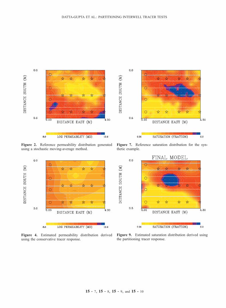
Figure 2. Reference permeability distribution generatedusing a stochastic moving-average method.

Figure 4. Estimated permeability distribution derivedusing the conservative tracer response.

Figure 7. Reference saturation distribution for the syn-thetic example.

Figure 9. Estimated saturation distribution derived usingthe partitioning tracer response.

15 - 7, 15 - 8, 15 - 9, and 15 - 10


Figure 11. Model assessment using resolution andcovariance analysis: (a) resolution of saturation estimatesand (b) variance of saturation estimates.

15 - 11 and 15 - 13

Figure 17. Hydraulic conductivity field estimated fromthe conservative tracer data for the Hill case (logpermeability scale).


Figure 21. NAPL saturation distribution estimated frompartitioning tracer data for the Hill case (cut-away view).

Figure 22. Spatial distribution of retardation factorscomputed at sampling locations.

Figure 23. Three-dimensional streamline pattern of thefinal model.

Figure 24. Tracer swept volume at various times (days).

15 - 14


15 - 15

Figure 26. Resolution of estimated NAPL saturation.

Figure 27. Region of high NAPL saturation distributionestimated using simulated annealing technique for the Hillcase.


Inverse modeling of partitioning interwell tracer … modeling of partitioning interwell tracer...

Documents

Transcript of Inverse modeling of partitioning interwell tracer … modeling of partitioning interwell tracer...