Analysis of Discontinuous Reception Power

Saving with Radio Resource Control States

Transition in LTE Networks

A THESIS Presented to

The Academic Faculty By

Cheng-Wen Hsueh

In Partial Fulfillment

of the Requirements for the Degree of

Master in Communications Engineering

Institute of Communications Engineering

College of Electrical and Computer Engineering

National Chiao Tung University

2013

Copyright c⃝2013 by Cheng-Wen Hsueh

Abstract

The 3GPP long term evolution(LTE) not only offer high bandwidth for data

transfer but also exhaust the User Equipment(UE)’s battery life quickly. In

order to save the UE’s battery Life, discontinuous reception(DRX) is speci-

fied to reduce the UE’s power consumption, DRX allow the UE to turn off

RF module when there is no data need to transfer. This work focus on anal-

ysis DRX mechanism with different RRC states, we use a simple numerically

analytical to model this. We divided the time period for power-saving opera-

tion into several independent parts to derive the power consumption and the

transmission delay. To analysis the power advisably, we introduce the real

power consumption through the power model. We evaluate the performance

that the UE is more power effectively when enters RRC IDLE in lower arrival

rate, and there is trade-off between the power and the transmission delay.

i

Acknowledgements

I would like to thank my parents and my younger sister. They always give

me endless supports. I especially thank Professor Li-Chun Wang and Li-Ping

Tung who gave me many valuable suggestions in my research during these

two years. I would not finish this work without his guidance and comments.

In addition, I am deeply grateful to my laboratory mates, Yim-Ming,

Shao-Heng, Yi-Cen, Gen-Hen, Si-Han and junior laboratory mates at Mo-

bile Communications and Cloud Computing Laboratory at the Graduate In-

stitute of Communications Engineering in National Chiao-Tung University.

They provide me with a lot of assistance and share happiness with me.

ii

Contents

Abstract i

Acknowledgements ii

Contents iii

List of Tables vi

List of Figures vii

1 Introduction 1

1.1 Problem and Solution . . . . . . . . . . . . . . . . . . . . . . . 3

1.1.1 Simple Analytical Model . . . . . . . . . . . . . . . . . 3

1.2 Thesis Outline . . . . . . . . . . . . . . . . . . . . . . . . . . . 4

2 Background 5

2.1 Literature Survey . . . . . . . . . . . . . . . . . . . . . . . . . 5

2.1.1 Discontinuous Reception(DRX) Mechanism Operation 6

2.1.2 Radio Resource Control(RRC) . . . . . . . . . . . . . . 8

2.1.3 UE’s Power Model in LTE . . . . . . . . . . . . . . . . 8

3 System Models 10

3.1 System Architecture . . . . . . . . . . . . . . . . . . . . . . . 10

iii

3.2 Active State and Sleeping State . . . . . . . . . . . . . . . . . 12

3.3 Immediate-Transmitting State and

Buffering-and-forwarding State . . . . . . . . . . . . . . . . . 13

3.4 Performance Metrics . . . . . . . . . . . . . . . . . . . . . . . 14

3.4.1 Power-saving Factor with Radio Resource Control States

Transition . . . . . . . . . . . . . . . . . . . . . . . . . 14

3.4.2 Real Power Consumption with Radio Resource Control

States Transition . . . . . . . . . . . . . . . . . . . . . 15

3.4.3 Transmission Delay with Radio Resource Control States

Transition . . . . . . . . . . . . . . . . . . . . . . . . . 15

4 Proposed Analytical Model 16

4.1 Assumptions . . . . . . . . . . . . . . . . . . . . . . . . . . . . 16

4.2 Definitions . . . . . . . . . . . . . . . . . . . . . . . . . . . . . 16

4.3 Power consumption . . . . . . . . . . . . . . . . . . . . . . . . 17

4.3.1 Power-saving Factor . . . . . . . . . . . . . . . . . . . 20

4.3.2 Real Power Consumption . . . . . . . . . . . . . . . . . 21

4.4 Transmission Delay . . . . . . . . . . . . . . . . . . . . . . . . 22

5 Simulation and Analytical Results 24

5.1 Power Consumption and Transmission Delay Verify Between

Simulation and Analytical Model . . . . . . . . . . . . . . . . 25

5.2 Analytical Parameters . . . . . . . . . . . . . . . . . . . . . . 26

5.3 Power-saving Factor with RRC States

Transition in Different CIDLE . . . . . . . . . . . . . . . . . . 27

5.4 Real Power Consumption with RRC

States Transition in Different CIDLE . . . . . . . . . . . . . . 27

iv

5.5 Transmission Delay with RRC States

Transition in Different CIDLE . . . . . . . . . . . . . . . . . . 28

5.6 Probability of the UE enters RRC IDLE . . . . . . . . . . . . 29

6 Conclusions 33

Bibliography 34

Vita 38

v

List of Tables

2.1 Comparison of Various Analytical Model in DRX operation. . 6

2.2 LTE power model. . . . . . . . . . . . . . . . . . . . . . . . . 9

vi

List of Figures

1.1 LTE network architecture between eNB and UE. . . . . . . . . 2

2.1 Illustration of LTE DRX operation in RRC CONNECTED. . 7

2.2 Different RRC states in LTE networks. . . . . . . . . . . . . . 9

3.1 3GPP LTE-A wireless networks DRX operation with RRC

states transition. . . . . . . . . . . . . . . . . . . . . . . . . . 11

5.1 Comparison between the analytical model and the simulation

results in different Power-saving factor with RRC states tran-

sition. . . . . . . . . . . . . . . . . . . . . . . . . . . . . . . . 25

5.2 Comparison between the analytical model and the simulation

results in different transmission delay with RRC states tran-

sition. . . . . . . . . . . . . . . . . . . . . . . . . . . . . . . . 26

5.3 Power-saving factor with RRC states transition (CIDLEDRX =

1000 ms). . . . . . . . . . . . . . . . . . . . . . . . . . . . . . 28

5.4 The trend of E[TL] and E[TIDLE] in different CIDLE. . . . . . 29

5.5 Real Power Consumption in 1 second. . . . . . . . . . . . . . . 30

5.6 Average packet transmission delay with RRC states transition

when N = 2 and CIDLEDRX = 1000 ms. . . . . . . . . . . . . . 31

5.7 Probability of the UE enters RRC IDLE. . . . . . . . . . . . . 32

vii

Chapter 1

Introduction

The fourth generation (4G) wireless technologies, such as Long Term Evo-

lution (LTE) of Universal Mobile Telecommunications System (UMTS) of-

fer high bandwidth for data transfer to support various applications. The

LTE has downlink peak date rate of 100Mbps and uplink peak data rate of

50Mbps by adopting some novel technologies (e.g., MIMO and OFDMA).

However, the high complexity of these new technologies may exhaust the UE

battery power quickly. Figure 1.1 shows LTE network architecture between

evolved Node B (eNB) and UE. In order to extend UE’s battery lifetime,

DRX is specified in 3GPP LTE standard to reduce the power consumption

of UE [1] [2]. In DRX operation, the UE periodically wakes up to monitor

new packet arrival in physical downlink control channel (PDCCH). If pack-

ets arrive, UE stays active until no more packets are received for a period of

time.

In [3–5], they considered the DRX operation with different channel con-

ditions, following the CQI to change the DRX parameters for performance

improvement. In [6–9], they introduced some ways to improvement VoIP

performance in the DRX operation. And the LaVoLTE is proposed in [10],

1

Figure 1.1: LTE network architecture between eNB and UE.

based on time series prediction and enhanced eNodeB architecture to deter-

mine DRX opportunities during video streaming over Real Time Protocol

(RTP) in a TDD-LTE network without compromising the QoS. In [11], to

power down energy consuming circuits in RF and BB, they proposed a Fast

Control Channel Decoding (FCCD) that the UE is not Nscheduled to receive

downlink data in the current TTI. In [12], they studied the characteristics

of different types of services. In [13], they introduced the DRX operation

under different RRC states. According to [14], RRC states has dramatically

impacts on UE’s power consumption and packet transmission delay. For the

performance of DRX, several analytical studies have been conducted. Yang

et al. [15, 16] proposed a Markov chain model of the DRX in UMTS system

where packet arrivals follow a Poisson process. Mihov et al. used semi-

Markov process to model the DRX in LTE system [17]. In [18], they use

the Markov model to build an algorithm that selects DRX parameters under

the QoS constraints. Jin and Qiao proposed an accurate analytical model to

2

avoid sophisticated steps [19].

DRX operation can manage UEs to achieve suitable battery consump-

tion in both RRC CONNECTED and RRC IDLE states in Evolved Univer-

sal Terrestrial Radio Access Network (E-UTRAN). Radio Resource Control

(RRC) is a protocol that communicates between the UE and the eNB, which

is part of LTE air interface control plane. It provides lots of functionalities,

such as paging, connection maintenance, security, QoS management, etc..

Under the same condition, UE may trigger different operations depending

on its RRC state. For example, if the signal quality from one neighboring

eNBs is better than the serving eNB, UE will trigger handover (HO) opera-

tion if the UE is in RRC CONNECTED state or perform a cell reselection if

the UE is in RRC IDLE state.

1.1 Problem and Solution

In this thesis, we focus on the DRX operation, and we also consider the

influence from RRC states transition, which is an important operation in

LTE system. We present a simple analytical model to analyze the efciency of

DRX operation and the inuence of the RRC states transition. Our proposed

model is similar to [19], but is more general in the 3GPP LTE-A power saving

operation since the RRC operation is taken into consideration.

1.1.1 Simple Analytical Model

To achieve this goal, we divide the DRX and RRC operations into several

parts, and we can derive them separately before we combine the results. As

the same as [15], we assume packet arrival intervals and transmission time

follow exponential and general distribution, respectively. The eNB allocates

3

a single-transmission RLC buffer for each UE, and the transmission buffer

size is infinite. To derive the power consumption, we divide the time period

into sleeping state with RRC states transition and active state. Then, we

can easily obtain the expected time duration of any state. Then, we can

have two results, i.e., power saving factor with RRC states transition and

real power consumption. We also derive the transmission delay by consider-

ing two states: immediate-transmitting state and buffering-and-forwarding

state. The immediate-transmitting state can be modeled by a M/G/1 queu-

ing system, and the buffering-and-forwarding state is derived, completely.

The analytical results show that there is much higher probability that the

UE enters RRC IDLE at lower packet arrival rate, and the power consump-

tion is relatively low at same time.

1.2 Thesis Outline

The rest of the article is organized as follows. We introduce the DRX op-

eration and the RRC states transition in Chapter 2. We also introduce our

system model in Chapter 3. Then, a analytical model has been proposed to

analyze the power consumption and the transmission delay in Chapter 4. To

verify our analytical, we simulate the DRX and RRC operation in Chapter 5.

The numerically results of analytical model are shown in Chapter 6. Finally,

Chapter 7 concludes this thesis.

4

Chapter 2

Background

In this chapter, we firstly survey related works to Discontinuous Recep-

tion(DRX) operation and Radio Resource Control(RRC) in LTE network.

Then, we introduce their operation in next two sections. And the power

model of UE is introduced in last section.

2.1 Literature Survey

DRX and RRC mechanisms will operate in different forms, which depends

on the characteristics of traffic. Consequently, it has impacts on UE’s power

consumption. For an effective investigation on the sufficiency of the LTE

DRX mechanisms, traffic analysis is of high importance. Thus, in [12], they

studied the characteristics of different types of services. In [13], they in-

troduced the DRX operation under different RRC states. According to [14],

RRC states has dramatically impacts on UE’s power consumption and packet

transmission delay. For the performance of DRX, several analytical studies

have been conducted. Yang et al. [15, 16] proposed a Markov chain model

of the DRX in UMTS system where packet arrivals follow a Poisson pro-

5

Table 2.1: Comparison of Various Analytical Model in DRX operation.

DRX Operation Queueing [15–17] Numerical [19] Our Proposed

DRX Parameters ◦ ◦ ◦

Power-saving Factor ◦ ◦ ◦

Transmission Delay ◦ ◦ ◦

Real Power Consumption × × ◦

Cross Layer Analysis × × ◦

cess. Mihov et al. used semi-Markov process to model the DRX in LTE

system [17]. In [18], they use the Markov model to build an algorithm that

selects DRX parameters under the QoS constraints. Jin and Qiao proposed

an accurate analytical model to avoid sophisticated steps [19].

2.1.1 Discontinuous Reception(DRX) Mechanism Op-

eration

In Evolved Universal Terrestrial Radio Access Network (E-UTRAN) Discon-

tinuous reception (DRX) is managed by the Radio Resource Control(RRC)

[1]. DRX is a process of turning off a radio receiver when it does not expect

to receive incoming messages. DRX can be enabled for UEs in RRC IDLE or

RRC CONNECTED mode. Here focus on the DRX in RRC CONNECTED

since in RRC IDLE state the UE does not have any sessions.

In RRC CONNECTED state, RRC controls DRX by configuring the

following parameters [2]: DRX inactivity timer (CI), DRX retransmission

timer, DRX start offset, On duration timer, long DRX cycle (CL), number

of short DRX cycle (N) and short DRX cycle (CS).

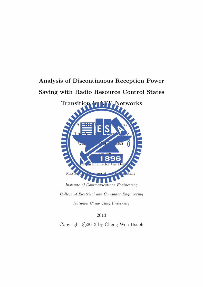
Figure 2.1 shows the LTE DRX operation in RRC CONNECTED.

6

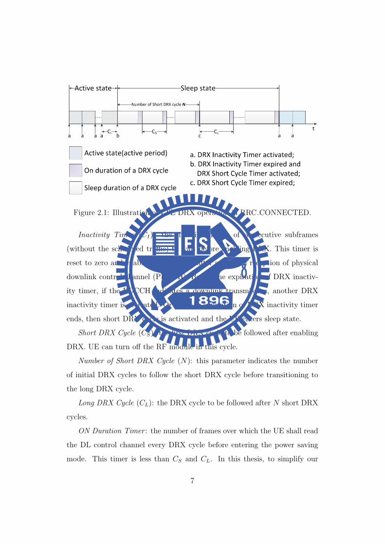
Figure 2.1: Illustration of LTE DRX operation in RRC CONNECTED.

Inactivity Timer (CI): the time in number of consecutive subframes

(without the scheduled traffic) to wait before enabling DRX. This timer is

reset to zero and enabled immediately after successful reception of physical

downlink control channel (PDCCH). Before the expiration of DRX inactiv-

ity timer, if the PDCCH indicates a downlink transmission, another DRX

inactivity timer is activated. Or else, the expiration of DRX inactivity timer

ends, then short DRX cycle is activated and the UE enters sleep state.

Short DRX Cycle (CS): the first DRX cycle to be followed after enabling

DRX. UE can turn off the RF module in this cycle.

Number of Short DRX Cycle (N): this parameter indicates the number

of initial DRX cycles to follow the short DRX cycle before transitioning to

the long DRX cycle.

Long DRX Cycle (CL): the DRX cycle to be followed after N short DRX

cycles.

ON Duration Timer : the number of frames over which the UE shall read

the DL control channel every DRX cycle before entering the power saving

mode. This timer is less than CS and CL. In this thesis, to simplify our

7

analytical model, we don’t consider this parameter.

DRX Offset : to obtain the starting subframe number for DRX cycle.

Retransmission Timer : the maximum number of subframes the UE should

wait before turning off the circuits if a retransmission of data is expected from

the eNB.

2.1.2 Radio Resource Control(RRC)

Radio Resource Control(RRC) protocol layer exists in UE and evolved node-

B(eNB), it is part of LTE air interface control plane. In DRX mode, the

UE powers down most of its circuitry when there are no packets to be trans-

mitted/received. During this time UE listens to the downlink (DL) occa-

sionally and may not keep in sync with uplink (UL) transmission depending

on whether the UE is registered with an eNB (RRC CONNECTED) or not

(RRC IDLE). In the RRC IDLE state, the UE is registered with the evolved

packet system (EPS) mobility management (EMM) but does not have an

active session. In this state the UE can be paged for DL traffic. UE can also

initiate UL traffic by requesting RRC connection with the serving eNB. In

the RRC CONNECTED state DRX mode is enabled during the idle periods

during the packet arrival process. Figure 2.2 shows different RRC states in

LTE networks.

2.1.3 UE’s Power Model in LTE

To calculate the real power consumption, we introduce a power model in

Table 2.2 [14]. We notice that the power consumption in RRC IDLE is much

lower than that in RRC CONNECTED. In addition, the network re-entry

time is denoted as TREENTRY to indicate the delay of the UE entering network

from RRC IDLE to RRC CONNECTED.

8

Figure 2.2: Different RRC states in LTE networks.

Table 2.2: LTE power model.

Power (mW) Duration (ms)

Short DRX On in RRC CONNECTED 1680.2±15.7 1.0±0.1

Long DRX On in RRC CONNECTED 1680.1±14.3 1.0±0.1

Off Duration in RRC CONNECTED 1060.0±3.3 N/A

Low power state in RRC IDLE 11.4±0.4 N/A

DRX On in RRC IDLE 594.3±8.7 TREENTRY :260.1

9

Chapter 3

System Models

Figure 3.1 shows the DRX operation with RRC state transition in 3GPP

LTE, we use active and sleeping (with RRC states transition) states to derive

the power consumption. As shown in this figure, we define four operational

states for proper analysis which is introduced upon. Additionally, we de-

fine activity period by the time duration from time instant that the Radio

Network Controller(RNC) begins to transmit packets under the condition

that the RNC is not transmitting packets in either active or sleeping state to

the time instant that RNCs buffer becomes empty due to the completion of

packet transmissions. The first activity period is defined by the activity pe-

riod, following DRX cycles. Meanwhile, the 3GPP LTE Advanced standard

specifies that the inactivity period is the time duration when an inactivity

timer is activated.

3.1 System Architecture

Two results are obtained as follow: One is the power-saving factor with RRC

states transition which is defined as the sleeping time over overall operation

10

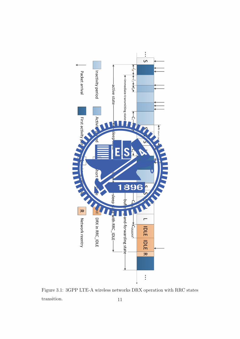
Figure 3.1: 3GPP LTE-A wireless networks DRX operation with RRC states

transition. 11

time. Furthermore, immediate-transmitting and buffering-and-forwarding

states are introduced to derive the transmission delay with RRC states tran-

sition.

3.2 Active State and Sleeping State

We first consider power-saving operation in the steady state. The steady-

state power-saving operation is divided into two stationary parts, i.e., the

operation in active and sleeping (with RRC states transition) states, respec-

tively. As we will explain later, the proposed approach gives us an easy way

to derive the expected time duration that the UE spends in each station-

ary part. Once we obtain the time durations in active and sleeping (with

RRC states transition) states, it is simple to have the power-saving factor.

Then, we continue to use these time durations to derive the average packet

transmission delay.

In active state, the UE receives packets during activity periods or waits

for new packet arrivals until inactivity timer timeout. For example, when

RNC’s buffer becomes empty after completing buffered packet transmissions,

the UE activates an inactivity timer prior to the beginning of sleeping state.

Unless there arrives a new packet within the timer expiration, the UE enters

sleeping state. Otherwise, a new activity period begins for the UE to receive

the newly arrived packets. The activity period can be extended as long as

more packets arrive at the RNC during ongoing packet transmission times.

Therefore, in active state, the activity period interleaved with the inactivity

period repeats until the inactivity timer expires.

And sleeping (with RRC states transition) state begins with the inactivity

timer’s expiration. In sleeping (with RRC states transition) states, the UE

12

monitors new packet arrivals by periodically receiving indication messages

every DRX cycle. If the UE notices new packet arrivals, the operational

state transits to active state for the UE to receive those packet during the

activity period. Optionally, a short cycle can be employed for more fre-

quent packet arrivals than a long DRX cycle. Long DRX cycle begins after

maximum number (N) of short DRX cycles has no receive any new packet.

When there is still no transmission of packets for an extended period of time,

(CIDLE), the eNB initiates RRC connection release. Accordingly, the UE

enters RRC IDLE state at same time.

3.3 Immediate-Transmitting State and

Buffering-and-forwarding State

After considering the power-saving operation in the steady state, we also

consider the transmission delay which is divided into two stationary parts,

i.e., immediate-transmitting state and buffering-and-forwarding state.

When the UE is in immediate-transmitting state, the packets suffers de-

lay due to residual time. Residual time is defined by the time required to

complete packet transmissions of all packets remaining in the transmission

buffer, as well as ongoing packet transmission when a packet arrives at an

arbitrary time. We find out that the delay due to the residual time is mod-

eled by a M/G/1 queuing system. The Pollaczek-Khinchine (PK) formula

presents packet transmission delay for a typical M/G/1 queuing system [20].

In buffering-and-forwarding state, the RNC does not transmit but buffers

packets during sleeping state and thereafter transmits the buffered pack-

ets during active state. By using the feature, we derive the delay for the

case when the UE is in buffering-and-forwarding state. Again, we apply the

13

M/G/1 queuing model to the derivation of packet transmission delay when

the RNC forwards buffered packets in buffering-and-forwarding state.

3.4 Performance Metrics

To analyze the DRX operation with RRC states transition aptly, we intro-

duce three types of definition, power-saving factor with radio resource control

states, transition, real power consumption with radio resource control states

transition and transmission delay with radio resource control states transi-

tion.

3.4.1 Power-saving Factor with Radio Resource Con-

trol States Transition

In the previous study [15–17,19,21], they use power-saving factor to analyze

the power consumption. The definition of the power-saving factor is the

percentage of time UE spends in sleep, which is an indicator of the power

saving performance the DRX mechanism achieves. It is formulated by

E[TD]

E[TA] + E[TD](3.1)

where TA is the time of UE stays in the active state, and TD is the UE stays

in DRX operation in RRC CONNECTED.

However, there has some different in our case. Due to consider the RRC

effect, we modify this factor and dene power saving factor with RRC states

transition as the sleeping time ratio, compared with the overall operation

time. Then, it can be formulated by

E[TD] + E[TIDLE]

E[TA] + E[TD] + E[TIDLE](3.2)

where TIDLE is the UE stays in RRC IDLE.

14

3.4.2 Real Power Consumption with Radio Resource

Control States Transition

In addition to power saving factor, we introduce a simple way to calculate the

real power consumption. pactive, pdrx and pidle are the power consumption in

three different states: active state, DRX in RRC CONNECTED, and DRX

in RRC IDLE, respectively, which can be obtained from the truly power

consumption, as shown in TABLE 2.2. Then, the real power consumption

with RRC states transition can be formulated by

1E[TA]+E[TD]+E[TIDLE ]

×(pactiveE[TA] + pdrxE[TD] + pidleE[TIDLE]).(3.3)

3.4.3 Transmission Delay with Radio Resource Con-

trol States Transition

The original definition of transmission delay is the waiting time of a packet

call delivery experiences before UE wakes up. In our case, we also consider

the RRC states transition in the transmission delay. To analyze delay more

aptly, the network re-entry time is denoted as TREENTRY to indicate the

delay of the UE entering network from RRC IDLE to RRC CONNECTED.

15

Chapter 4

Proposed Analytical Model

4.1 Assumptions

We assume that packet arrival intervals are modeled as an exponentially dis-

tributed random variable with mean 1/λ, and transmission times are general

distribution with E[X] = τ for a single packet. The traffic intensity ρ = λτ .

In addition, we know that the number of packet arrivals can be modeled

with the Poisson process since packet arrivals follow an exponential distribu-

tion. Then, we simply derive the average number packet arrivals during the

transmission time for a single packet by∞∑n=0

(λτ)n

n!e−λτ = λτ = ρ.

4.2 Definitions

Random variable t̂I represents the time of inactivity timer which starts when

there is no data to transmit but stops due to a new packet arrival. Random

variable tB represents the subsequent activity period after the inactivity timer

stops. Random variable t̃B represents the transmission time for the buffered

packets during the last sleep state before the first activity period. Random

16

variable TA, TD and TIDLE indicate the times that the UE stays in active

state, DRX operation state, and RRC IDLE state. According to 3GPP LTE

specification, CI , CS, CL, CIDLEDRX represent inactivity timer, short DRX

cycle, long DRX cycle, and DRX cycle in RRC IDLE. Considering the impact

of situation where the UE enters RRC IDLE state, we adopt CIDLE as the

control timer from RRC CONNECTED to RRC IDLE.

4.3 Power consumption

To analyze the power aptly, we introduce two types of definitions, power-

saving factor with RRC states transition and real power consumption. For

this purpose, we have to derive E[TA], E[TD], and E[TIDLE]. First, the power-

saving factor with RRC states transition is formulated by

E[TD] + E[TIDLE]

E[TA] + E[TD] + E[TIDLE]. (4.1)

The duration of active state will be extended when there are some packets

arrived before inactivity timer (CI) expires, and the inactivity timer will

restart again. Accordingly, we can derive the new packet arrival probability

by∫ CI

0λe−λtdt = 1− e−λCI . The duration of sleep state can be derived in the

similar way. When there are some packets arrived within the short DRX cycle

(CS) or long DRX cycle (CL), the UE will enter active state and the timer will

stop counting. Otherwise, the time period of sleeping state will be extended.

Thus, we can derive the probability of the UE staying in short DRX cycle by∫∞CS

λe−λtdt = e−λCS on the condition of no packet arrived within the short

DRX cycle. The probability of the UE staying in long DRX cycle can be

derived by∫∞CL

λe−λtdt = e−λCL , similarly. The probabilities of the UE leaving

active state, short DRX cycle, and long DRX cycle can also be derived by 1−

17

∫ CI

0λe−λtdt = e−λCI , 1−e−λCS , and 1−e−λCL , respectively. Additionally, we

derive the probability of the UE leaving RRC IDLE by 1−∫∞CIDLE

λe−λtdt =

1 − e−λCIDLE . The sleeping state with RRC IDLE consists of short DRX

cycle, long DRX cycle, and the duration of RRC IDLE. After figuring out

these independent probabilities, we can represent the probabilities of active

state and sleeping state with RRC IDLE, respectively.

Probability of active state αi

we adopt i to indicate how many times of inactivity timer restarts, which

means there is still new packet arrived before inactivity timer expires. The

probability of active state can be derived by

αi = (1− e−λCI )ie−λCI (4.2)

where i ≥ 0.

Probability of sleeping state with RRC IDLE δj

we adopt j to indicate the number of short and long DRX cycles. To indicate

CIDLE by unit of short DRX cycle, L = (CIDLE −CS)/CL is used to replace

the time of the UE staying in long DRX cycle, then N +L is the total cycle

of short and long DRX cycles. The probabilities of the sleep state can be

derived by (4.3).

δ

λ λ

j

C j Ce eS S

=

−− − −( ) ( ),

11 1 << ≤

− < ≤ +− − − + −

−

j N

e e e N j N L

e

C N C j N C

C

S L L

S

( ) ( ) ( ),

(

( )λ λ λ

λ

11

)) ( ) ( ),N C L C

e e N L jL IDLE− −− + <

λ λ

1

(4.3)

18

Now, to derive the time durations for active state and sleeping state with

RRC IDLE, we assume that E[tS] and E[tL] are the average time where short

and long DRX cycles last, and E[tIDLE] is the average time of the UE staying

in RRC IDLE. Therefore, we have

E[TA] = E[t̃B] +∞∑0

iαi(E[t̂I ] + E[tB]) + CI

= E[t̃B] + (E[t̂I ] + E[tB])(eλCI − 1) + CI

(4.4)

E T E T E t E t E t

j e e C

D IDLE S L IDLE

C j C

SS S

[ ] [ ] [ ] [ ] [ ]

( ) ( )

+ = + +

= −− − −λ λ1

1jj

N

C N C j N

j N

N L

C

L

j N e e

e C

j

S L

L

=

− − − +

= +

+

−

∑

∑+ −

× −

+

1

1

1

1

( )( ) ( )

( )

(

( )λ λ

λ

−− +

× −

−

= + +

∞

− −

∑ ( ))( )

( ) ( )

N L e

e e C

C N

j N L

C L C

IDLEDRX

S

L IDLE

λ

λ λ

1

1

(4.5)

Now, we proceed to derive E[t̂I ], E[t̃B] and E[tB]. Since t̂I follows a

truncated exponential distribution, the probability density function (pdf)

f(t) is given by

f t ee t C

C t

C

t

I

I

I( ),

, .

= −≤ ≤

<

−

−1

10

0

λ

λλ

(4.6)

19

Then, we can derive E[t̂I ] by

E[t̂I ] =∫∞0

tf(t)dt

= 1λ− 1

eλCI−1CI .

(4.7)

Random variable tB starts when there is a new packet arrived and it will

continue until all the buffered packets have been transmitted. Besides, we

can model the number of packet arrivals as the Poisson process since packet

arrivals follow an exponential distribution. Then, we can derive the av-

erage packet arrivals during the transmission time for a single packet by∞∑n=0

(λτ)n

n!e−λτ = λτ = ρ. It means that a single packet transmission produces

additional ρ packets. In addition, it need τρ transmission time. Eventually,

we got E[tB] by

E[tB] =∞∑n=0

τρn =τ

1− ρ. (4.8)

Accordingly, random variable t̃B can be derived as the same way. t̃B indi-

cates the first time period to transmit the packets buffered during the DRX

cycle or RRC IDLE state. We introduce λ(E[TD]+E[TIDLE]) to indicate the

number of packets buffered at the beginning during the sleeping state with

RRC IDLE, and we can derive E[t̃B] by

E[t̃B] = λ(E[TD] + E[TIDLE])τ

1− ρ= (E[TD] + E[TIDLE])

ρ

1− ρ(4.9)

4.3.1 Power-saving Factor

Now, we can summarize the power-saving factor with RRC states transition

as

20

E T E T

E T E T E T

E T E T

E

D IDLE

D IDLE A

D IDLE

[ ] [ ]

[ ] [ ] [ ]

( [ ] [ ])( )

(

++ +

=+ −1 ρ

[[ ] [ ]) ( )

( ) ( )

(

T E T e

j e e C

j

D IDLE

C

C j C

S

j

N

I

S S

+ + −

=

−

+ −

− − −

=∑

11

11

1

λλ

λ λ

NN e e e C

j N L e

C N C j N C

j N

N L

LS L L)( ) ( ) ( )

( ( ))(

( )− − − + −

= +

+

−

−

+ − +

∑ λ λ λ1

1

1

λλ λ λC N C L C

j N L

IDLEDRXS L IDLEe e C) ( ) ( )

− −

= + +

∞

−

∑ 11

−

−

+ −

− − −

=

− −

∑

( )

( ) ( )

( )( ) (

1

11

1

ρ

λ λ

λ λ

j e e C

j N e e

C j C

S

j

N

C N C

S S

S L )) ( )

( ( ))( ) ( ) (

( )j N C

j N

N L

L

C N C L

e C

j N L e e

L

S L

− + −

= +

+

− −

−

+ − + −

∑ 1

1

1

1

λ

λ λee C

e

C

j N L

IDLEDRX

C

IDLE

I

−

= + +

∞

∑

+ −

λ

λ

λ

)

( )

1

11

..

(4.10)

4.3.2 Real Power Consumption

In addition to power-saving factor, we introduce a simple way to calculate the

real power consumption. pactive, pdrx and pidle are the power consumption in

three different states: active state, DRX in RRC CONNECTED, and DRX

in RRC IDLE, respectively, which can be obtained from the truly power

consumption, as shown in TABLE 2.2. Then, the real power consumption

with RRC states transition can be formulated by

1E[TA]+E[TD]+E[TIDLE ]

×(pactiveE[TA] + pdrxE[TD] + pidleE[TIDLE]).(4.11)

21

4.4 Transmission Delay

In order to analyze the transmission delay with RRC states transition, we

adopt the methodology proposed in [19] to divide whole operation into immed-

iate-transmitting state and buffering-and-forwarding state. In immediate-

transmitting state, we introduce a typical M/G/1 queuing system with Pollac-

zek-Khinchine formula to simply derive the average packet transmission delay

(E[DI ]) [20]. The result is

E[DI ] =λE[X2]

2(1− ρ). (4.12)

In buffering-and-forwarding state, we consider two types of delay: the

residual time, which can be solved as (4.12), similarly, and the packet buffer-

ing operation during the DRX cycle or RRC IDLE state. These two types of

delay resulted from the packets arrived during the DRX cycle or RRC IDLE.

To calculate the average number of waiting packet, we introduce two nota-

tions, E[K] and E[W ]. E[K] is the average number of waiting packet in

transmission buffer, and E[W ] is the average waiting time since packet ar-

rived during the DRX cycle or RRC IDLE. Then we can derive the packet

buffering operation by

E[DB] = E[W ] + E[X]E[K] (4.13)

where E[K] = λE[DB], which is obtained from Little’s Law. And we can

derive E[DB] by

E[DB] = E[W ] + E[X]E[K]

= E[W ] + λτE[DB]

= E[W ] + ρE[DB]

= E[W ]1−ρ

.

(4.14)

When there are one or more packet arrivals during the DRX cycle or

RRC IDLE, it will start the first active period after the cycle ends. Such

22

cycle becomes the last DRX cycle in sleeping state (with RRC IDLE). So we

need to derive the average time that the arrival packets in the last DRX cycle

until the first active period starts. The packet arrival time in the last cycle is

uniform distribution, which follows the property of the Poisson process [22].

According to the packets arrive at the DRX cycle or RRC IDLE, we can

obtain E[W ] = CS/2 (or CL/2) or CIDLEDRX/2. In addition, the network

re-entry time is denoted as TREENTRY to indicate the delay of the UE entering

network from RRC IDLE to RRC CONNECTED. The probabilities of the

packets suffering from delay can be derived by

PS =E[tS]

E[TA] + E[TD] + E[TIDLE](4.15)

PL =E[tL]

E[TA] + E[TD] + E[TIDLE](4.16)

PIDLE =E[tIDLE]

E[TA] + E[TD] + E[TIDLE](4.17)

From (4.12)-(4.17), we can obtain the average transmission delay with

RRC states transition by

E D P P P E D

P E DC

P E DC

S L IDLE I

S I

S

L I

L

[ ] ( ) [ ]

( [ ]( )

) ( [ ](

= − − −

+ +−

+ +

1

2 1 2ρ 11

2 1

1

2

−

+ +−

+

= +

ρ

ρ

))

( [ ]( )

)

[ ][ ]

P E DC

T

E DE t C

IDLE I

IDLEDRX

REENTRY

I

S SS L L IDLE IDLEDRX

D IDLE

C

ID

E t C E t C

E T E T e

P

I

+ +

+ + −

+

[ ] [ ]

( [ ] [ ] ( ))1 1λ λ

LLE RNENTRYT .

(4.18)

23

Chapter 5

Simulation and Analytical

Results

To confirm correctness of the analytical model, we verify the analytical model

by comparing analytical results with simulation results. We develop a simula-

tor to simulate DRX operation with RRC states transition which is written by

Java. For Simulation parameters, we have expected transmission time(τ), av-

erage packet arrival rate(λ),InactivityTimer(CI), short DRX cycle(CS), long

DRX cycle(CL), number of short DRX cycle(N), expended period of time

that UE enters RRC IDLE when there is no transmission of packets(CIDLE),

DRX cycle in RRC IDLE(CIDLEDRX) and network re-entry time TREENTRY .

24

5.1 Power Consumption and Transmission De-

lay Verify Between Simulation and Ana-

lytical Model

We simulate different CIDLE to compare with the analytical model. As shown

in Figure 5.1 and Figure 5.2, acceptable-matched results show that numerical

equations are correctly derived. But there still has some mismatch which is

caused by our simulator neglects some complicate factor. So the simulator

still have to be improved actuality.

0.8

0.82

0.84

0.86

0.88

0.9

0.92

0.94

0.96

0.0005 0.001 0.0015 0.002 0.0025

Pow

er

Savin

g F

acto

r

Packet Arrival Rates (1/ms)

Ana. at CIDLE=1.2sSim. at CIDLE=1.2sAna. at CIDLE=2.4sSim. at CIDLE=2.4sAna. at CIDLE=3.6sSim. at CIDLE=3.6s

Figure 5.1: Comparison between the analytical model and the simulation

results in different Power-saving factor with RRC states transition.

25

100

150

200

250

300

350

400

450

500

0.0005 0.001 0.0015 0.002 0.0025

Tra

nsm

issio

n D

ela

y (

ms)

Packet Arrival Rates (1/ms)

Ana. at CIDLE=1.2sSim. at CIDLE=1.2sAna. at CIDLE=2.4sSim. at CIDLE=2.4sAna. at CIDLE=3.6sSim. at CIDLE=3.6s

Figure 5.2: Comparison between the analytical model and the simulation

results in different transmission delay with RRC states transition.

5.2 Analytical Parameters

To evaluate the impact of condition where UE enters RRC IDLE state; in

this chapter, we use MATLAB tool to obtain the numerical results from our

derived model.The corresponding parameters are set as follows. We have

packet transmission time τ = 0.1ms, DRX InactivityTimer CI = 100ms,

short DRX cycle CS = 200ms, long DRX cycle CL = 400ms, and network

re-entry time TREENTRY = 260ms, which is setting by [14].

26

5.3 Power-saving Factor with RRC States

Transition in Different CIDLE

The power-saving factor with RRC states transition is illustrate in Figure 5.3.

When CIDLE = 1.2s, the UE will enter RRC IDLE with higher probability

at lower packet arrival rate. Nevertheless, when CIDLE = 4.8s, the UE will

enter RRC IDLE with lower probability even at lower packet arrival rate.

So we can manifest the UE is more power efficiency when CIDLE = 1.2s.

The effect of E[TIDLE] can be neglected when packet arrival rate increase

gradually. According to the reason that the power consumption is dramatic

different between RRC IDLE and RRC CONNECTED, which is illustrated

in TABLE 2.2, we propose another way to indicate the power consumption

appropriately.

To explain the reason why the power-saving factor in CIDLE = 1.2s, Figure

5.4 shows the trend of E[TL] and E[TIDLE] in different CIDLE, we can realize

E[TL] is more outstanding than E[TIDLE] when the DRX effect increases.

5.4 Real Power Consumption with RRC

States Transition in Different CIDLE

To indicate the effect of power consumption, we calculate the real power

consumption based on TABLE 2.2. In Figure 5.5, we observe that the time

for the UE to enter RRC IDLE become longer at lower packet arrival rate;

it implies real power consumption is relatively low. In addition, power con-

sumption is increased when CIDLE = 4.8s, which is different from the trend

of power-saving factor, as shown in Figure 5.3. It is obviously to see that the

real power consumption model can express more reality than power-saving

27

0.8

0.82

0.84

0.86

0.88

0.9

0.92

0.94

0.96

0.0005 0.001 0.0015 0.002 0.0025

Pow

er

Savin

g F

acto

r

Packet Arrival Rates (1/ms)

CIDLE=1.2sCIDLE=2.4sCIDLE=3.6sCIDLE=4.8s

Figure 5.3: Power-saving factor with RRC states transition (CIDLEDRX =

1000 ms).

factor in this situation. And we can know if the user uses some applications

like web or other some non-GBR(Guranteed Bit Rate) services, we suggest

the CIDLE can set in 1 or 2 seconds which can be more power-saving when

the UE can stays in RRC IDLE for longer time.

5.5 Transmission Delay with RRC States

Transition in Different CIDLE

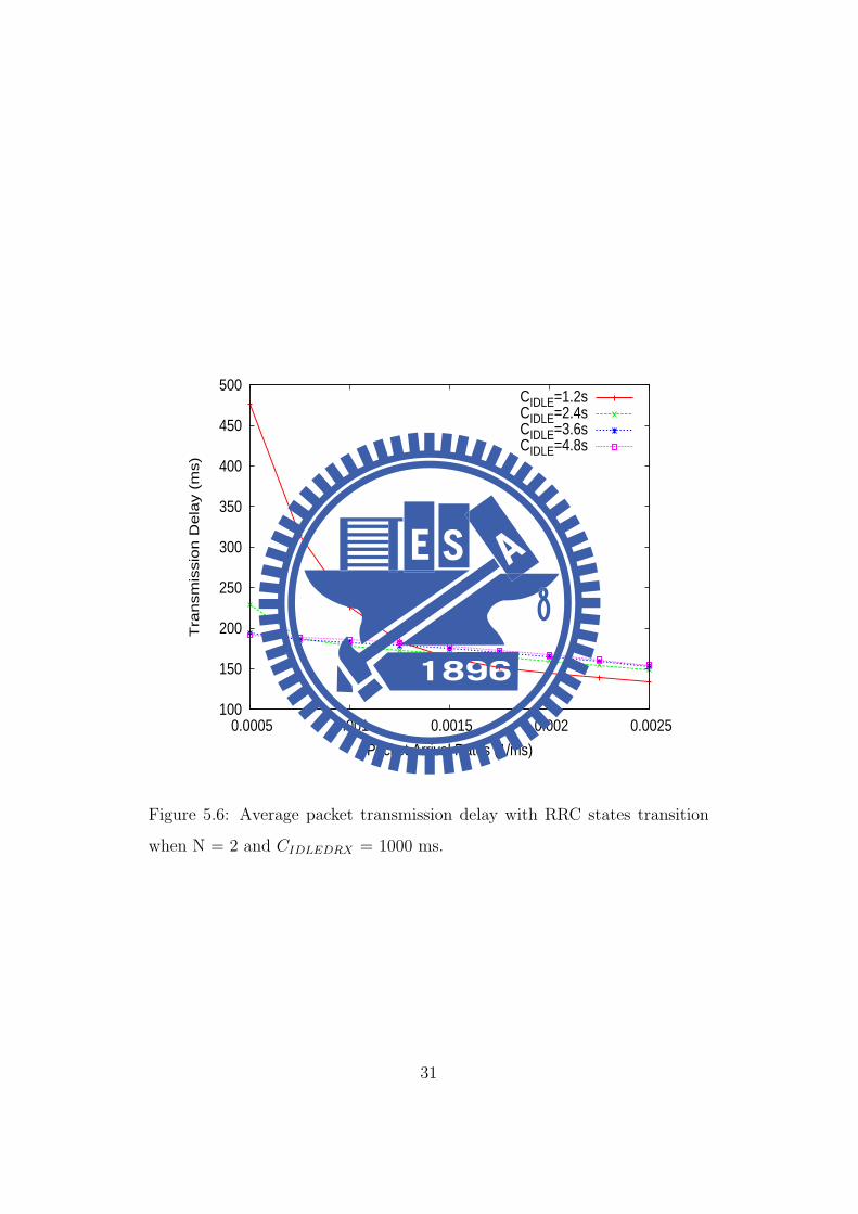
Figure 5.6 depicts the average transmission delay under different packet ar-

rival rate λ. The average transmission delay decreases as the packet arrival

28

0

500

1000

1500

2000

2500

1500 2000 2500 3000 3500 4000 4500

Tim

e P

eriod(m

s)

CIDLE Time(ms)

TLTIDLE

Figure 5.4: The trend of E[TL] and E[TIDLE] in different CIDLE.

rate increases since the UE stays in RRC IDLE state for shorter time. Fur-

thermore, Figure 5.5 and Figure 5.6 show that there is a trade-off between

the transmission delay and the real power consumption. And due to there

is much higher delay when the UE enters RRC IDLE, the applications like

VoIP or other some GBR services do not aptly to enters RRC IDLE.

5.6 Probability of the UE enters RRC IDLE

We use Figure 5.7 as an evidence to show that the probability of staying in

RRC IDLE state for UE decreases as the the packet arrival rate increases.

It implies that there is a high probability of entering the RRC IDLE state

when UE with lower packet arrival rate.

29

600

700

800

900

1000

1100

1200

1300

0.0005 0.001 0.0015 0.002 0.0025

Real P

ow

er

Consum

ption (

J)

Packet Arrival Rates (1/ms)

CIDLE=1.2sCIDLE=2.4sCIDLE=3.6sCIDLE=4.8s

Figure 5.5: Real Power Consumption in 1 second.

30

100

150

200

250

300

350

400

450

500

0.0005 0.001 0.0015 0.002 0.0025

Tra

nsm

issio

n D

ela

y (

ms)

Packet Arrival Rates (1/ms)

CIDLE=1.2sCIDLE=2.4sCIDLE=3.6sCIDLE=4.8s

Figure 5.6: Average packet transmission delay with RRC states transition

when N = 2 and CIDLEDRX = 1000 ms.

31

0

0.1

0.2

0.3

0.4

0.5

0.6

0.0005 0.001 0.0015 0.002 0.0025

Pro

babili

ty

Packet Arrival Rates (1/ms)

CIDLE=1.2sCIDLE=2.4sCIDLE=3.6sCIDLE=4.8s

Figure 5.7: Probability of the UE enters RRC IDLE.

32

Chapter 6

Conclusions

In this thesis, in order to realize the impact of RRC states transition on

DRX mechanism, we derive some numerical functions to model this effect

from simple probability theory. By dividing the DRX and RRC operations

into several independent parts, we can calculate them separately and then

combine the result eventually. We obtain the power saving factor with RRC

effect, real power consumption, and packet transmission delay. The analyt-

ical results show that there is a trade-off between the power consumption

and transmission delay, which has also been verified. Furthermore, under

lower packet traffic arrival rate, the UE enters RRC IDLE states with higher

probability, thus it can save much more power. This work can be extended

to determine the best DRX and RRC operation parameters.

33

Bibliography

[1] 3GPP TR 36.321 V11.2.0, Evolved Universal Terrestrial Radio Access

(E-UTRA); Medium Access Control (MAC) Protocol Specification (Re-

lease 11), 3rd Generation Partnership Project Std., March 2013.

[2] 3GPP TR 36.331 V11.3.0, Evolved Universal Terrestrial Radio Access

(E-UTRA); Radio Resource Control (RRC); Protocol specification (Re-

lease 11), 3rd Generation Partnership Project Std., March 2013.

[3] L. Liu, X. She, and L. Chen, “Multi-user and Channel Dependent

Scheduling Based Adaptive Power Saving for LTE and Beyond System,”

in 16th Asia-Pacific Conference on Communications (APCC), 2010, pp.

118–122.

[4] K. Aho, J. Puttonen, T. Henttonen, and L. Dalsgaard, “Channel Quality

Indicator Preamble for Discontinuous Reception,” in IEEE 71st Vehic-

ular Technology Conference(VTC Spring), 2010, pp. 1–5.

[5] S. Gao, H. Tian, J. Zhu, and L. Chen, “A more Power-efficient Adaptive

Discontinuous Reception Mechanism in LTE,” in Proc. IEEE Vehicular

Technology Conference (VTC Fall), 2011, pp. 1–5.

34

[6] Y. Fan, P. Lunden, M. Kuusela, and M. Valkama, “Efficient Semi-

persistent Scheduling for VoIP on Eutra Downlink,” in Vehicular Tech-

nology Conference, 2008. VTC 2008-Fall. IEEE 68th, 2008, pp. 1–5.

[7] K. Aho, I. Repo, T. Nihtila, and T. Ristaniemi, “Analysis of VoIP Over

HSDPA Performance With Discontinuous Reception Cycles,” in Sixth

International Conference on Information Technology: New Generations(

ITNG ’09), 2009, pp. 1190–1194.

[8] K. Aho, T. Henttonen, J. Puttonen, and T. Ristaniemi, “Trade-off Be-

tween Increased Talk-time and LTE Performance,” in Ninth Interna-

tional Conference on Networks (ICN), 2010, pp. 371–375.

[9] M. Polignano, D. Vinella, D. Laselva, J. Wigard, and T. Sorensens,

“Power Savings and QoS Impact for VoIP Application with DRX/DTX

Feature in LTE,” in Proc. IEEE 73rd Vehicular Technology Confer-

ence(VTC Spring), 2011, pp. 1–5.

[10] R. Kalle, A. Nandan, and D. Das, “La VoLTE: Novel Cross Layer Opti-

mized Mechanism of Video Transmission Over LTE for DRX,” in Proc.

IEEE 75th Vehicular Technology Conference(VTC Spring), 2012, pp.

1–5.

[11] M. Lauridsen, A. Jensen, and P. Mogensen, “Fast Control Channel De-

coding for LTE UE Power Saving,” in Proc. IEEE 75th Vehicular Tech-

nology Conference(VTC Spring), 2012, pp. 1–5.

[12] S. Baghel, K. Keshav, and V. Manepalli, “An Investigation Into Traf-

fic Analysis for Diverse Data Applications on Smartphones,” in Proc.

National Conference Communications (NCC), 2012, pp. 1–5.

35

[13] C. Bontu and E. Illidge, “DRX Mechanism for Power Saving in LTE,”

Communications Magazine, IEEE, vol. 47, no. 6, pp. 48–55, 2009.

[14] J. Huang, F. Qian, A. Gerber, Z. M. Mao, S. Sen, and O. Spatscheck, “A

Close Examination of Performance and Power Characteristics of 4G LTE

Networks,” in Proc. 10th International Conference on Mobile Systems,

Applications, and Services, 2012, pp. 225–238.

[15] S.-R. Yang and Y.-B. Lin, “Modeling UMTS Discontinuous Reception

Mechanism,” IEEE Transactions on Wireless Communications,, vol. 4,

no. 1, pp. 312–319, 2005.

[16] S.-R. Yang, S.-Y. Yan, and H.-N. Hung, “Modeling UMTS Power Sav-

ing with Bursty Packet Data Traffic,” IEEE Transactions on Mobile

Computing, vol. 6, no. 12, pp. 1398–1409, 2007.

[17] Y. Mihov, K. Kassev, and B. Tsankov, “Analysis and Performance Eval-

uation of the DRX Mechanism for Power Saving in LTE,” in IEEE 26th

Convention of Electrical and Electronics Engineers in Israel (IEEEI),

2010, pp. 000 520–000 524.

[18] Y.-P. Yu and K.-T. Feng, “Traffic-based DRX Cycles Adjustment

Scheme for 3GPP LTE Systems,” in Proc. IEEE 75th Vehicular Tech-

nology Conference(VTC Spring), 2012.

[19] S. Jin and D. Qiao, “Numerical Analysis of the Power Saving in 3GPP

LTE Advanced Wireless Networks,” IEEE Transactions Vehicular Tech-

nology, vol. 61, no. 4, pp. 1779–1785, 2012.

[20] H. Takagi, Queueing Analysis: A Foundation of Performance Evalua-

tion. North-Holland, 1991.

36

[21] L. Zhou, H. Xu, H. Tian, Y. Gao, L. Du, and L. Chen, “Performance

Analysis of Power Saving Mechanism with Adjustable DRX Cycles in

3GPP LTE,” in Vehicular Technology Conference, 2008. VTC 2008-Fall.

IEEE 68th, 2008, pp. 1–5.

[22] S. M. Ross, Stochastic Processes. Wiley, 1983.

37

Vita

Cheng-Wen Hsueh

He was born in Taiwan, R. O. C. in 1989. He received a B.S. in De-

partment of Electronic Engineering from Chung Yuan Christian University

in 2011. From July 2011 to August 2013, he worked his Master degree in

the Mobile Communications and Cloud Computing Lab in the Department

of Communication Engineering at National Chiao-Tung University. His re-

search interests are in the field of wireless communications and mobile com-

puting.

38