Analysis of biological networks:Random Models∗

Lecturer: Roded Sharan Scribe: Ori Folger and Keren Yizhak

Lecture 2, March 11, 2009

In this lecture we discuss fundamental concepts in network analysis and present random network models.

1 Concepts

We begin with introducing important concepts in network analysis.

1.1 Random (ER) graphs

The Erdos-Renyi (ER) random graphs model, also called simply random graphs, was presented by Erdosand Renyi [4] in the 1950s and 1960s. Erdos and Renyi characterized random graphs and showed that manyof the properties of such networks can be calculated analytically.

Construction of an ER random graph with parameter 0 ≤ p ≤ 1 and N nodes is by connecting everypair of nodes with probability p. Note that the resulting graph is a simple graph.

Figure 1: Source [4]. Degree distribution of a random graph, and an example of such a graph.

1.2 Scale-free networks

Many complex networks found in the real world feature an important property - most nodes have a fewlinks to other nodes, but a small number of nodes are highly connected and have a huge number of links toother nodes. This leads to the observation that these networks do not have nodes with a typical number ofneighbors, and in this sense these networks are scale-free. The modern investigation of scale-free networksbegan with Barabasi and Albert[2].

In order to analyze these networks, we require several definitions. The degree sequence for a graph isdefined as the vector (d(1), d(2), . . . , d(n)) holding the degree information d(v) of each node v in the graph.

∗Based on a scribe by: Elena Kyanovsky, David Hadas, Lior Gavish and Ory Samorodnitzky.

1

The degree distribution for a graph, denoted by P (k), is defined to be the fraction of nodes in the graph witha degree k. The degree distribution can be calculated thus:

P (k) =| {v|d(v) = k} |

N(1)

where d(v) is the degree of node v and N is the number of nodes in the graph. A network can be characterizedin terms of its degree distribution. A directed graph has two separate degree distributions, namely the in-degree distribution and the out-degree distribution.

The average degree in a graph is denoted d ≡∑

k kP (k). Note that the number of edges in the graph isgiven by m = Nd

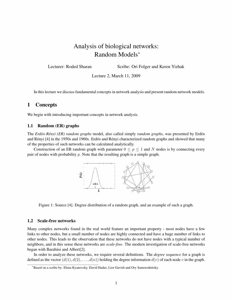
2 .The degree distribution of several real networks is shown in Figure 2. All of these networks display a

power-law degree distribution, which is defined by:

P (k) ∝ k−c, k 6= 0, c > 1 (2)

The constraint c > 1 ensures the proper convergence of the total probability, i.e. the sum∑∞

k=1 P (k). Intypical networks, c takes values in the range 2 ≤ c ≤ 3.

Figure 2: Source: [1]. The degree distributions of several real networks. The graphs are log-log graphswhere both axes use a logarithmic scale. (a) Internet router connections; (b) movie actor collaborations; (c)co-authorship network of high-energy physicists; (d) co-authorship network of neuroscientists. Note howthe graphs are near linear, indicating a power-law function.

And just as in the real networks, in a power-law degree distribution there are many nodes with lowdegrees and a small number of nodes with high degrees. The high degree nodes are highly important to thenetwork connectivity and serve as hubs.

The term scale-free is also justified by the power-law degree distribution, since it can be scaled withoutaltering the distribution. If we denote the distribution by p(k), scaling the distribution by a factor a resultsin p(ak) = g(a)p(k), which means that the distribution looks the same in every range of k. Thus, thepower-law distribution has no natural scale and is scale-invariant (in fact, this is the only distribution withthis property).

2

1.3 Clustering coefficient

An important measure of network cohesiveness is the clustering coefficient. As shown in Watts and Stro-gatz [10], in many complex networks we find clusters which are subsets of the network that display a highlevel of inner connectivity. The clustering coefficient measures the degree of clustering of a typical node’sneighborhood. It is defined as the likelihood that any two nodes with a common neighbor are themselvesconnected. For example, in a friends network, it is the likelihood that two persons who have a common ac-quaintance also know each other. The clustering coefficient is a local property which describes the networkstructure of nodes which are close to each other.

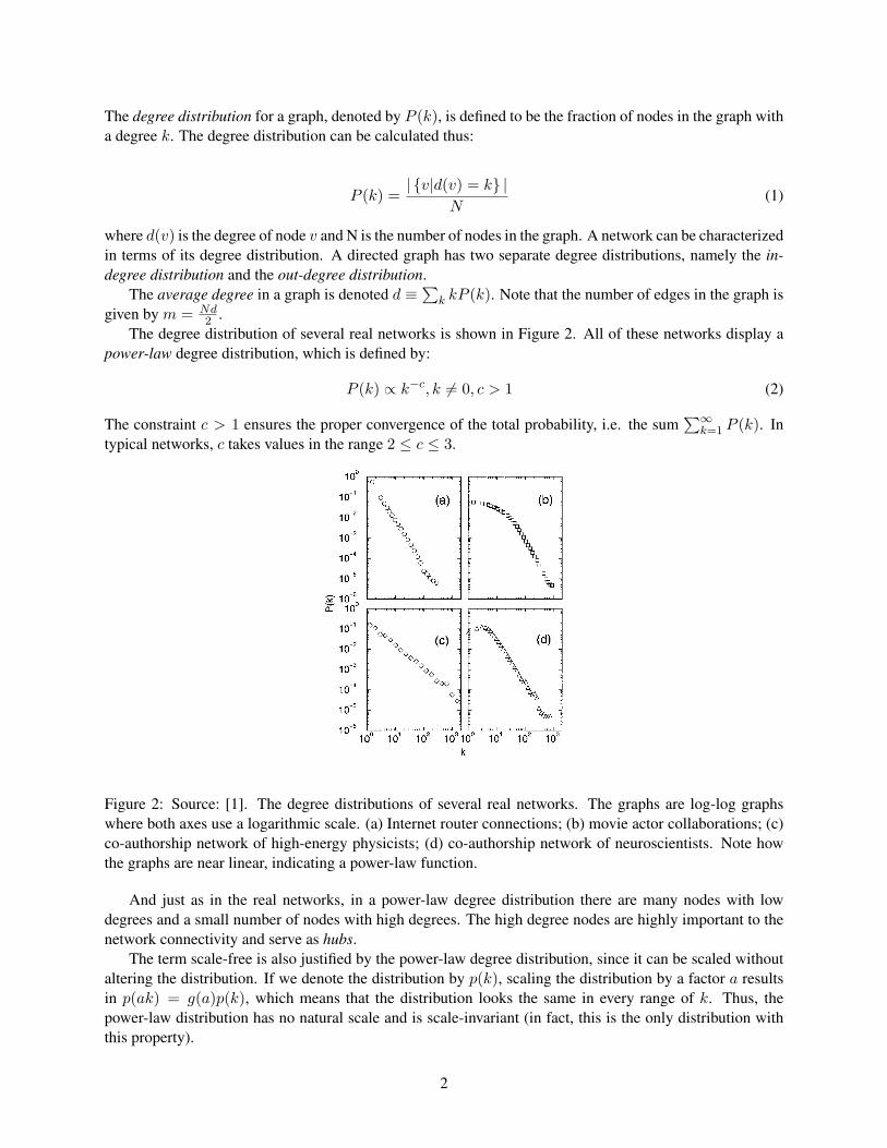
To calculate the clustering coefficient, we first define the node clustering coefficient, C(v), of a node v,as the proportion of pairs of connected neighbors of v out of the total number of pairs of neighbors of v.Every such pair of neighbors, for example u and w, forms a triangle with v, a cycle of length 3 (see figure3). Let t(v) be the number of triangles containing v. Then C(v) can be calculated by

C(v) =t(v)

12d(v)(d(v)− 1)

(3)

Where we define for d(v) = 0 and for d(v) = 1 that C(v) = 0.

Figure 3: Calculating the clustering coefficient of a node. The node v has degree d = 6, and participates int(v) = 3 triangles. Therefore, C(v) = 3

12∗6∗5 = 1

5 .

The network clustering coefficient, C, is defined as the average of C(v) over all nodes in the network:

C =1N

∑v

C(v) (4)

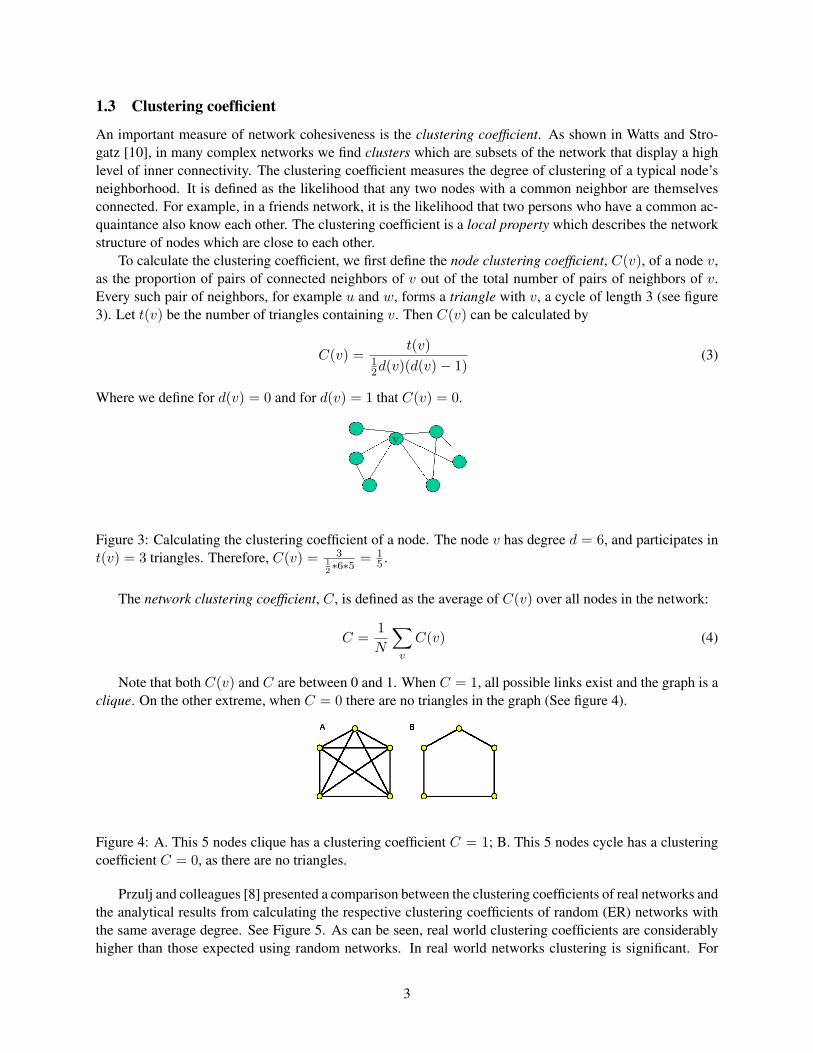
Note that both C(v) and C are between 0 and 1. When C = 1, all possible links exist and the graph is aclique. On the other extreme, when C = 0 there are no triangles in the graph (See figure 4).

Figure 4: A. This 5 nodes clique has a clustering coefficient C = 1; B. This 5 nodes cycle has a clusteringcoefficient C = 0, as there are no triangles.

Przulj and colleagues [8] presented a comparison between the clustering coefficients of real networks andthe analytical results from calculating the respective clustering coefficients of random (ER) networks withthe same average degree. See Figure 5. As can be seen, real world clustering coefficients are considerablyhigher than those expected using random networks. In real world networks clustering is significant. For

3

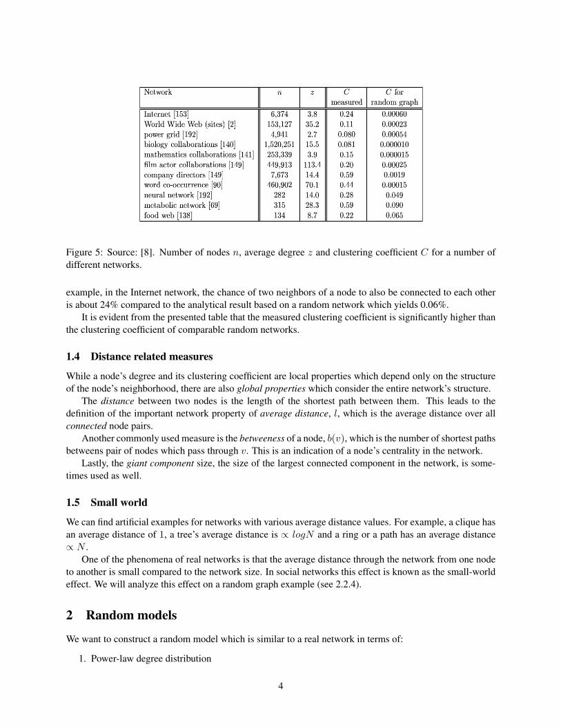
Figure 5: Source: [8]. Number of nodes n, average degree z and clustering coefficient C for a number ofdifferent networks.

example, in the Internet network, the chance of two neighbors of a node to also be connected to each otheris about 24% compared to the analytical result based on a random network which yields 0.06%.

It is evident from the presented table that the measured clustering coefficient is significantly higher thanthe clustering coefficient of comparable random networks.

1.4 Distance related measures

While a node’s degree and its clustering coefficient are local properties which depend only on the structureof the node’s neighborhood, there are also global properties which consider the entire network’s structure.

The distance between two nodes is the length of the shortest path between them. This leads to thedefinition of the important network property of average distance, l, which is the average distance over allconnected node pairs.

Another commonly used measure is the betweeness of a node, b(v), which is the number of shortest pathsbetweens pair of nodes which pass through v. This is an indication of a node’s centrality in the network.

Lastly, the giant component size, the size of the largest connected component in the network, is some-times used as well.

1.5 Small world

We can find artificial examples for networks with various average distance values. For example, a clique hasan average distance of 1, a tree’s average distance is ∝ logN and a ring or a path has an average distance∝ N .

One of the phenomena of real networks is that the average distance through the network from one nodeto another is small compared to the network size. In social networks this effect is known as the small-worldeffect. We will analyze this effect on a random graph example (see 2.2.4).

2 Random models

We want to construct a random model which is similar to a real network in terms of:

1. Power-law degree distribution

4

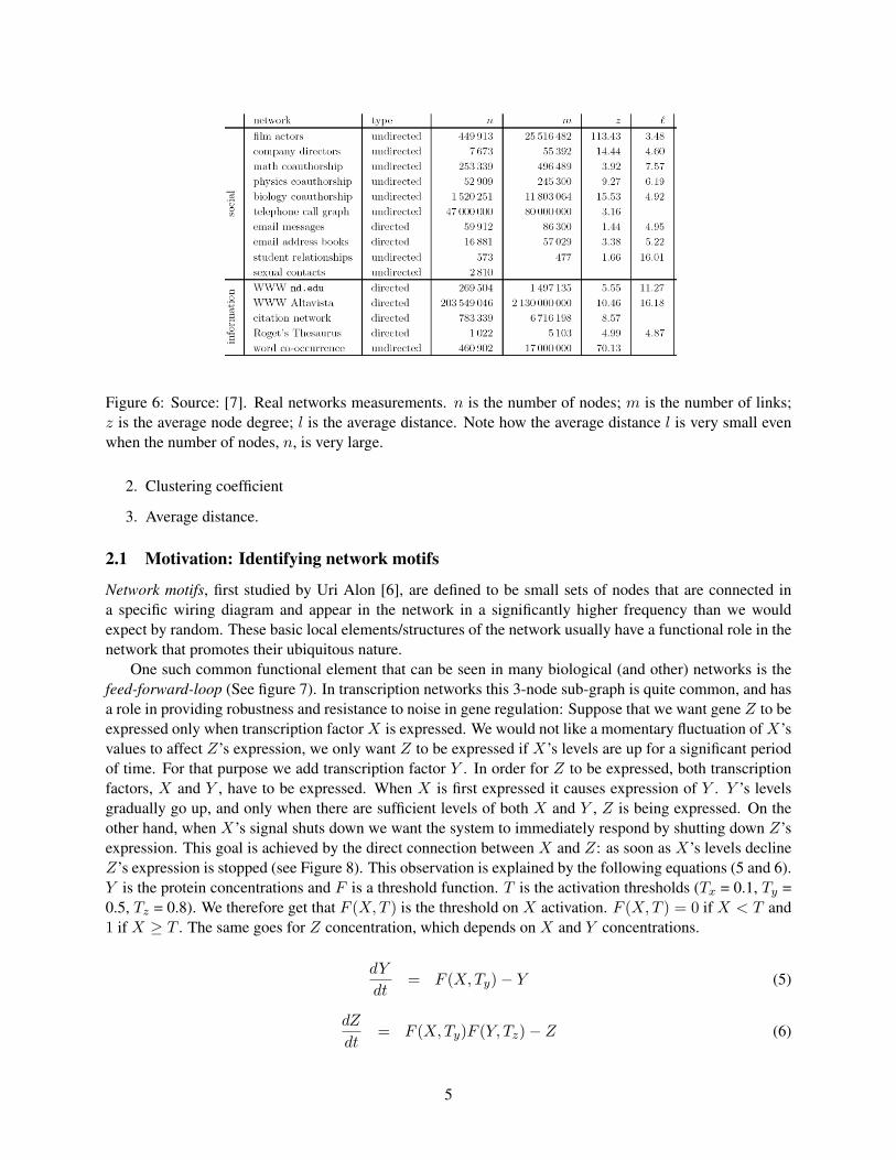
Figure 6: Source: [7]. Real networks measurements. n is the number of nodes; m is the number of links;z is the average node degree; l is the average distance. Note how the average distance l is very small evenwhen the number of nodes, n, is very large.

2. Clustering coefficient

3. Average distance.

2.1 Motivation: Identifying network motifs

Network motifs, first studied by Uri Alon [6], are defined to be small sets of nodes that are connected ina specific wiring diagram and appear in the network in a significantly higher frequency than we wouldexpect by random. These basic local elements/structures of the network usually have a functional role in thenetwork that promotes their ubiquitous nature.

One such common functional element that can be seen in many biological (and other) networks is thefeed-forward-loop (See figure 7). In transcription networks this 3-node sub-graph is quite common, and hasa role in providing robustness and resistance to noise in gene regulation: Suppose that we want gene Z to beexpressed only when transcription factor X is expressed. We would not like a momentary fluctuation of X’svalues to affect Z’s expression, we only want Z to be expressed if X’s levels are up for a significant periodof time. For that purpose we add transcription factor Y . In order for Z to be expressed, both transcriptionfactors, X and Y , have to be expressed. When X is first expressed it causes expression of Y . Y ’s levelsgradually go up, and only when there are sufficient levels of both X and Y , Z is being expressed. On theother hand, when X’s signal shuts down we want the system to immediately respond by shutting down Z’sexpression. This goal is achieved by the direct connection between X and Z: as soon as X’s levels declineZ’s expression is stopped (see Figure 8). This observation is explained by the following equations (5 and 6).Y is the protein concentrations and F is a threshold function. T is the activation thresholds (Tx = 0.1, Ty =0.5, Tz = 0.8). We therefore get that F (X, T ) is the threshold on X activation. F (X, T ) = 0 if X < T and1 if X ≥ T . The same goes for Z concentration, which depends on X and Y concentrations.

dY

dt= F (X, Ty)− Y (5)

dZ

dt= F (X, Ty)F (Y, Tz)− Z (6)

5

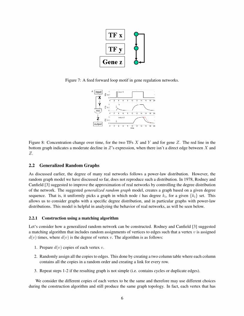
Figure 7: A feed forward loop motif in gene regulation networks.

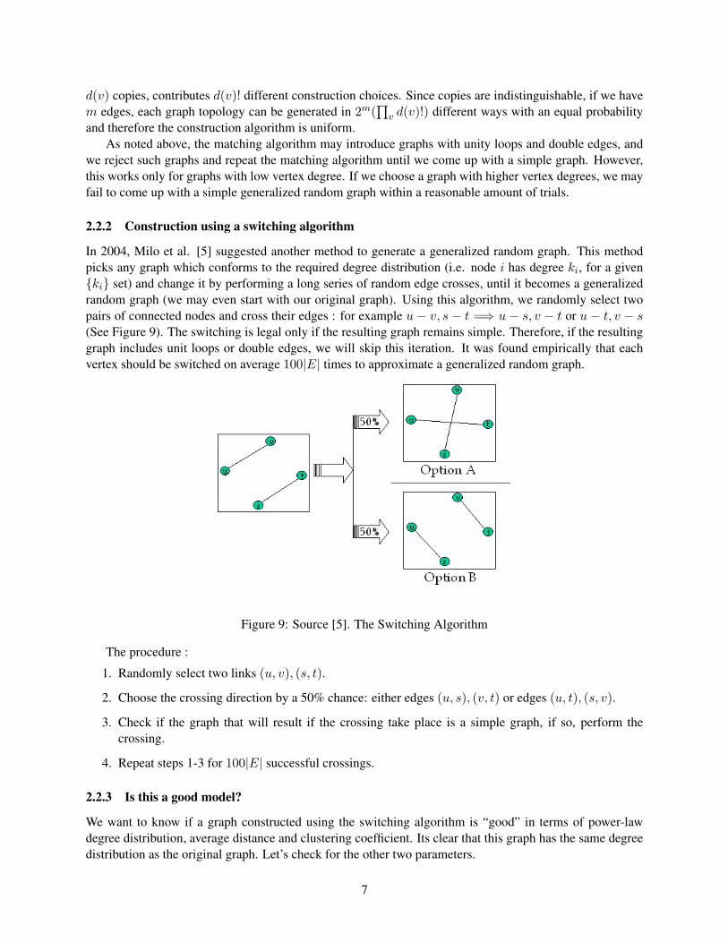
Figure 8: Concentration change over time, for the two TFs X and Y and for gene Z. The red line in thebottom graph indicates a moderate decline in Z’s expression, when there isn’t a direct edge between X andZ.

2.2 Generalized Random Graphs

As discussed earlier, the degree of many real networks follows a power-law distribution. However, therandom graph model we have discussed so far, does not reproduce such a distribution. In 1978, Rodney andCanfield [3] suggested to improve the approximation of real networks by controlling the degree distributionof the network. The suggested generalized random graph model, creates a graph based on a given degreesequence. That is, it uniformly picks a graph in which node i has degree ki, for a given {ki} set. Thisallows us to consider graphs with a specific degree distribution, and in particular graphs with power-lawdistributions. This model is helpful in analyzing the behavior of real networks, as will be seen below.

2.2.1 Construction using a matching algorithm

Let‘s consider how a generalized random network can be constructed. Rodney and Canfield [3] suggesteda matching algorithm that includes random assignments of vertices to edges such that a vertex v is assignedd(v) times, where d(v) is the degree of vertex v. The algorithm is as follows:

1. Prepare d(v) copies of each vertex v.

2. Randomly assign all the copies to edges. This done by creating a two column table where each columncontains all the copies in a random order and creating a link for every row.

3. Repeat steps 1-2 if the resulting graph is not simple (i.e. contains cycles or duplicate edges).

We consider the different copies of each vertex to be the same and therefore may use different choicesduring the construction algorithm and still produce the same graph topology. In fact, each vertex that has

6

d(v) copies, contributes d(v)! different construction choices. Since copies are indistinguishable, if we havem edges, each graph topology can be generated in 2m(

∏v d(v)!) different ways with an equal probability

and therefore the construction algorithm is uniform.As noted above, the matching algorithm may introduce graphs with unity loops and double edges, and

we reject such graphs and repeat the matching algorithm until we come up with a simple graph. However,this works only for graphs with low vertex degree. If we choose a graph with higher vertex degrees, we mayfail to come up with a simple generalized random graph within a reasonable amount of trials.

2.2.2 Construction using a switching algorithm

In 2004, Milo et al. [5] suggested another method to generate a generalized random graph. This methodpicks any graph which conforms to the required degree distribution (i.e. node i has degree ki, for a given{ki} set) and change it by performing a long series of random edge crosses, until it becomes a generalizedrandom graph (we may even start with our original graph). Using this algorithm, we randomly select twopairs of connected nodes and cross their edges : for example u − v, s − t =⇒ u − s, v − t or u − t, v − s(See Figure 9). The switching is legal only if the resulting graph remains simple. Therefore, if the resultinggraph includes unit loops or double edges, we will skip this iteration. It was found empirically that eachvertex should be switched on average 100|E| times to approximate a generalized random graph.

Figure 9: Source [5]. The Switching Algorithm

The procedure :

1. Randomly select two links (u, v), (s, t).

2. Choose the crossing direction by a 50% chance: either edges (u, s), (v, t) or edges (u, t), (s, v).

3. Check if the graph that will result if the crossing take place is a simple graph, if so, perform thecrossing.

4. Repeat steps 1-3 for 100|E| successful crossings.

2.2.3 Is this a good model?

We want to know if a graph constructed using the switching algorithm is “good” in terms of power-lawdegree distribution, average distance and clustering coefficient. Its clear that this graph has the same degreedistribution as the original graph. Let’s check for the other two parameters.

7

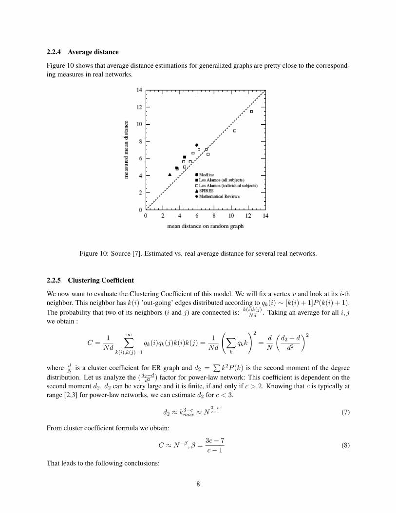
2.2.4 Average distance

Figure 10 shows that average distance estimations for generalized graphs are pretty close to the correspond-ing measures in real networks.

Figure 10: Source [7]. Estimated vs. real average distance for several real networks.

2.2.5 Clustering Coefficient

We now want to evaluate the Clustering Coefficient of this model. We will fix a vertex v and look at its i-thneighbor. This neighbor has k(i) ’out-going’ edges distributed according to qk(i) ∼ [k(i) + 1]P (k(i) + 1).The probability that two of its neighbors (i and j) are connected is: k(i)k(j)

Nd . Taking an average for all i, jwe obtain :

C =1

Nd

∞∑k(i),k(j)=1

qk(i)qk(j)k(i)k(j) =1

Nd

(∑k

qkk

)2

=d

N

(d2 − d

d2

)2

where dN is a cluster coefficient for ER graph and d2 =

∑k2P (k) is the second moment of the degree

distribution. Let us analyze the (d2−dd2 ) factor for power-law network: This coefficient is dependent on the

second moment d2. d2 can be very large and it is finite, if and only if c > 2. Knowing that c is typically atrange [2,3] for power-law networks, we can estimate d2 for c < 3.

d2 ≈ k3−cmax ≈ N

3−cc−1 (7)

From cluster coefficient formula we obtain:

C ≈ N−β , β =3c− 7c− 1

(8)

That leads to the following conclusions:

8

• When c = 7/3 there is a phase transition.

• When c > 7/3 - C tends to 0 with increasing of N

• When c < 7/3 - C increases with graph size

Thus, for a good random graph network model we expect cluster coefficient to be 2 < c < 3.

2.2.6 Summary

We have given an introduction to the use of random graphs as models of real-world networks and evaluateddifferent properties for such a model. Most scale-free networks have cluster coefficient between 2 < c < 3and a giant component emerges when c > 3.4788 (see [7]). Though there are certain drawbacks that differrandom graphs from real networks, this model is very popular and is the best studied model.

2.3 A biologically motivated scale-free random model

The models described so far focus on the topology of the network and not on its dynamics. Some of thesemodels predict scale-free features and some of them do not; the random graph model do not reproduce apower-law degree distribution. However, we can construct generalized random graphs that have a power-lawdegree distribution, but not proper clustering coefficients.

All of these models leave open an important question: what is the mechanism responsible for the emer-gence of scale-free networks? The scale-free model, suggested by Barabasi and Albert [2], tries to answerthis question and is based on two observations:

• Real networks are hardly fixed, and they evolve and grow through time.

• In real networks, connections are not uniform and some vertices tend to have more connections asnew vertices prefer to attach themselves to them. E.g., in a citation network (where each vertex is anarticle and there is a directed edge from an article to another article iff it refers to it) a popular articletends to have more references from new articles as compared to non-popular ones.

Barabasi and Albert introduced a model that is based upon these two definitions:

1. Growth - The network starts from m0 vertices and it grows as new nodes are added. Each addedvertex has degree m (m0 ≥ m). The fixed degree is a reasonable assumption for some networks, suchas the scientific citation network. In that network, most articles have a fixed number of referenceswhich does not vary much. In case the degree for the new vertex is fixed (m), the average degree inthe graph after growth is 2m, as each of the new m edges is counted for two vertices (after growth,the initial degrees of the first m0 vertices can be ignored, as m0 � N ).

2. Preferential attachment - The probability that a new vertex will connect to an existing vertex, is notuniform. Rather, it is proportional to its degree. I.e, if d(v) is the degree of vertex v, then:

P (u connects to v) =d(v)∑d(v)

(9)

Preferential attachment can be explained in biological networks by gene duplication. For example,we take the protein-protein interaction (PPI) network, where each protein is a vertex, and two proteinsare connected iff they can interact with each other. During evolution, a gene may be duplicated,leading to a duplication of the protein it encodes. Assuming duplication preserves interactions, thenew duplicated protein will have interactions with all the neighbors of the original protein. This leadsto preferential attachment, as more connected proteins will gain more new neighbors.

9

2.3.1 Empirical evidences

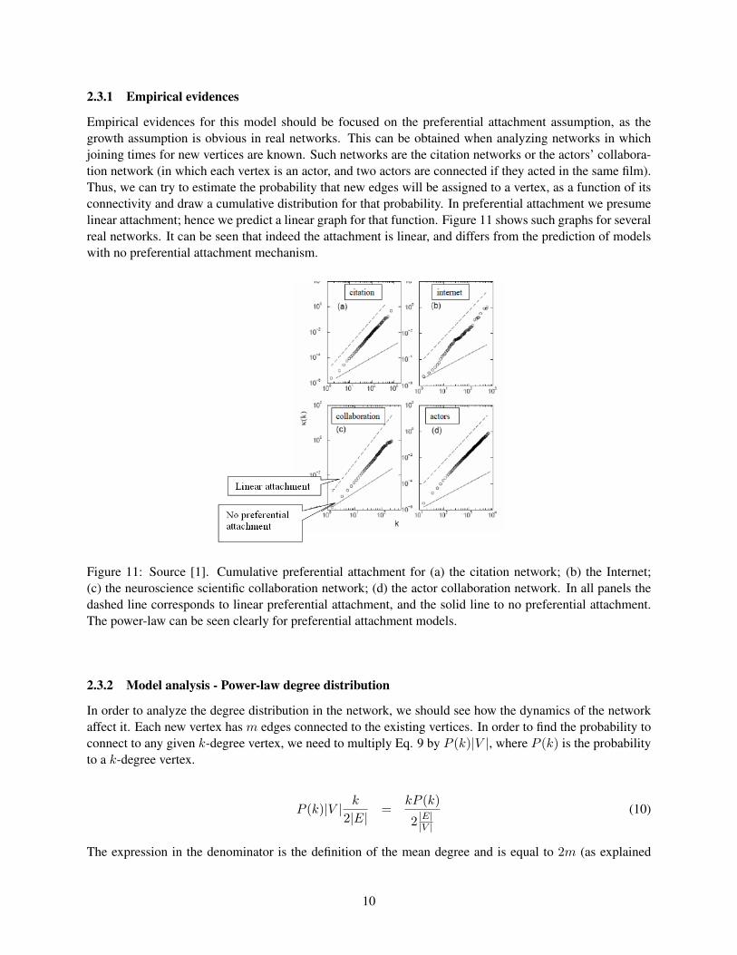
Empirical evidences for this model should be focused on the preferential attachment assumption, as thegrowth assumption is obvious in real networks. This can be obtained when analyzing networks in whichjoining times for new vertices are known. Such networks are the citation networks or the actors’ collabora-tion network (in which each vertex is an actor, and two actors are connected if they acted in the same film).Thus, we can try to estimate the probability that new edges will be assigned to a vertex, as a function of itsconnectivity and draw a cumulative distribution for that probability. In preferential attachment we presumelinear attachment; hence we predict a linear graph for that function. Figure 11 shows such graphs for severalreal networks. It can be seen that indeed the attachment is linear, and differs from the prediction of modelswith no preferential attachment mechanism.

Figure 11: Source [1]. Cumulative preferential attachment for (a) the citation network; (b) the Internet;(c) the neuroscience scientific collaboration network; (d) the actor collaboration network. In all panels thedashed line corresponds to linear preferential attachment, and the solid line to no preferential attachment.The power-law can be seen clearly for preferential attachment models.

2.3.2 Model analysis - Power-law degree distribution

In order to analyze the degree distribution in the network, we should see how the dynamics of the networkaffect it. Each new vertex has m edges connected to the existing vertices. In order to find the probability toconnect to any given k-degree vertex, we need to multiply Eq. 9 by P (k)|V |, where P (k) is the probabilityto a k-degree vertex.

P (k)|V | k

2|E|=

kP (k)

2 |E||V |

(10)

The expression in the denominator is the definition of the mean degree and is equal to 2m (as explained

10

above). We therefore get:

kP (k)2m

(11)

As each new vertex has m edges, in order to estimate the number of vertices with k-degree that will gainnew edges from the new vertex, we should multiply the expression in (11) by m. Thus, we get:

mkP (k)2m

=kP (k)

2(12)

which is independent of m. From the above expression we can learn about the dynamics of the degreedistribution in the network. We shall now investigate the degree distribution in the transition between anetwork with N vertices to a network of N + 1 vertices. Denote P (k, N) as the probability for a k-degreevertex in a network with N vertices. When a new vertex is added, kp(k)/2 vertices with k degree will gainanother edge and will become (k+1)-degree vertices, and the new network will contain N +1 vertices. If wetake k = m (the minimal degree), we deduce that in the transition from N to N + 1 vertices, mP (m,N)/2vertices become with degree m + 1, and one m-degree vertex is added - the new vertex. Therefore, fork = m, the net change in the above transition is:

(N + 1)P (m,N + 1)−NP (m,N) = 1− mP (m, N)2

(13)

For k > m two effects should be considered: the number of k− 1 degree vertices that gained a new edge tobecome k-degree vertices and the number of k-degree vertices that gained a new edge and became of degreek + 1. Therefore, for k > m the net change in the transition is:

(N + 1)P (k, N + 1)−NP (k, N) =(k − 1)P (k − 1, N)− kP (k, N)

2(14)

When looking for a stationary degree distribution, which is independent of N , we have

P (k, N + 1) = P (k, N) = P (k)

Solving this recursive formulae yields to the following expression:

P (k) =

(k−1)P (k−1)−kP (k)

2 k > m

1− mP (m)2 k = m

(15)

From Eq. 15 we get

2P (k) + kP (k) = (k − 1)P (k − 1) (16)

P (k) =(k − 1)P (k − 1)

(k + 2)(17)

11

Eq. 17 is the recursion formula and if we expand the recursion up till k = m we will come up with:

P (k) =k − 1k + 2

P (k − 1) =k − 1k + 2

· k − 2k + 1

P (k − 2) =

k − 1k + 2

· k − 2k + 1

k − 3k

P (k − 3) =k − 1k + 2

· k − 2k + 1

k − 3k

k − 4k − 1

P (k − 4) =

k − 1k + 2

· k − 2k + 1

k − 3k

k − 4k − 1

· · · m

m + 2· 2m + 2

=

2m(m + 1)k(k + 1)(k + 2)

We can see that expressions eliminate each other and in the limit of large k this gives a power-law degreedistribution, P (k) ∼ k−3.

2.3.3 Model analysis - Clustering coefficient

Empirical analysis of the Barabasi-Albert model shows that the clustering coefficient C decreases with thenetwork size, following approximately a power-law C ∼ N− 3

4 . Figure 12 shows that this is a more moderateslope to that observed in random graphs (where C ∼ N−1). However, it is still converges to 0 when weincrease N .

Figure 12: Source [1]. Clustering coefficient versus size of the Barabasi- Albert model with k = 4,compared with the clustering coefficient of a random graph.

2.4 Geometric Random Graphs

2.4.1 Definition

We define a geometric graph, G(V, r) above a metric space S and a distance measure δ, to be the graph withnode set V of points in S and edge set:

E = {(u, v)|(u, v ∈ V ) ∧ (0 < δ(u, v) ≤ r)} (18)

12

That is, points in a metric space correspond to nodes and two nodes are adjacent if the distance betweenthem is at most r. r is called the radius of the graph.A random geometric graph, G(n, r) above a metric space S and a distance measure δ, is a geometric graphwith radius r on n nodes which were chosen randomly and independently from a uniform distribution overthe points in S. For example, we can choose the two dimensional unit square to be our metric space and theEuclidean distance (2-norm) as the distance measure.

2.4.2 Global graph properties

As usual, we evaluate how good of a real-world network model a geometric random graph is by taking intoconsideration three global graph properties: degree distribution, average distance and clustering coefficient.Two out of these three standard network parameters show an improved fit to a GRN (Geometric RandomNetwork) than to the popular scale-free model.

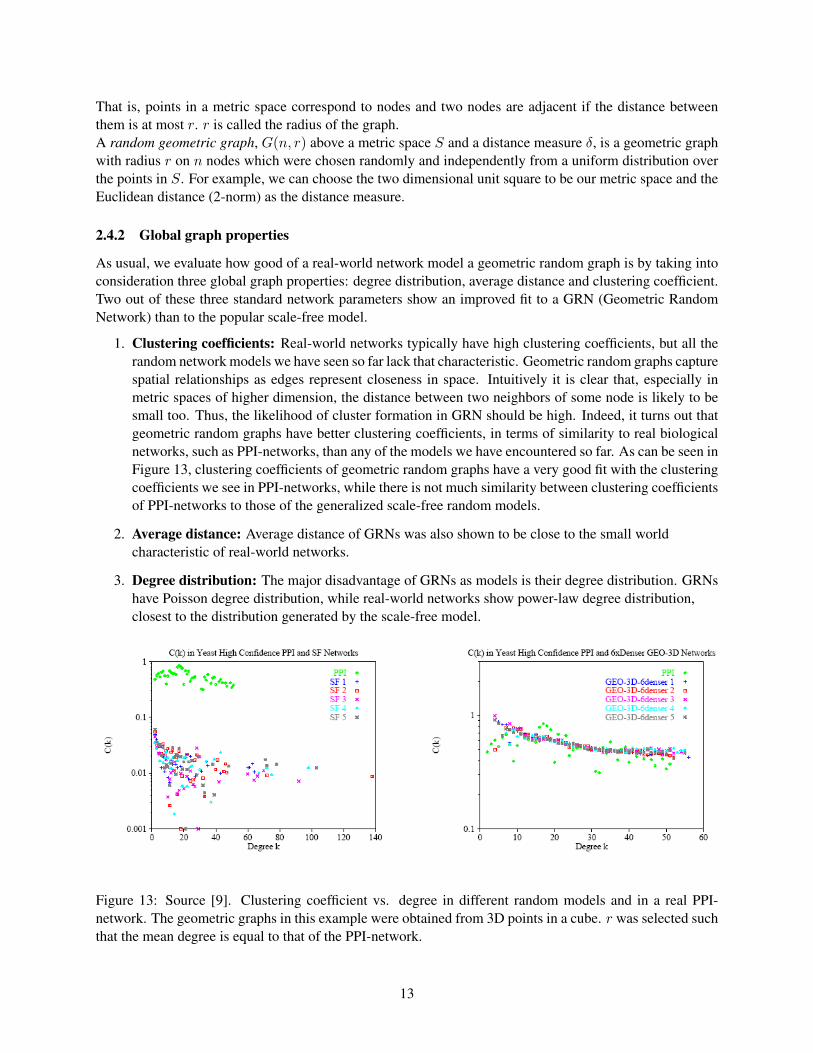
1. Clustering coefficients: Real-world networks typically have high clustering coefficients, but all therandom network models we have seen so far lack that characteristic. Geometric random graphs capturespatial relationships as edges represent closeness in space. Intuitively it is clear that, especially inmetric spaces of higher dimension, the distance between two neighbors of some node is likely to besmall too. Thus, the likelihood of cluster formation in GRN should be high. Indeed, it turns out thatgeometric random graphs have better clustering coefficients, in terms of similarity to real biologicalnetworks, such as PPI-networks, than any of the models we have encountered so far. As can be seen inFigure 13, clustering coefficients of geometric random graphs have a very good fit with the clusteringcoefficients we see in PPI-networks, while there is not much similarity between clustering coefficientsof PPI-networks to those of the generalized scale-free random models.

2. Average distance: Average distance of GRNs was also shown to be close to the small worldcharacteristic of real-world networks.

3. Degree distribution: The major disadvantage of GRNs as models is their degree distribution. GRNshave Poisson degree distribution, while real-world networks show power-law degree distribution,closest to the distribution generated by the scale-free model.

Figure 13: Source [9]. Clustering coefficient vs. degree in different random models and in a real PPI-network. The geometric graphs in this example were obtained from 3D points in a cube. r was selected suchthat the mean degree is equal to that of the PPI-network.

13

2.4.3 Local graph properties

Local graph properties, such as small, over represented patterns, may be important and characteristic to thenetwork’s (biological) function. Thus, it is important that our model will be able to imitate local propertiesof real-life networks too.

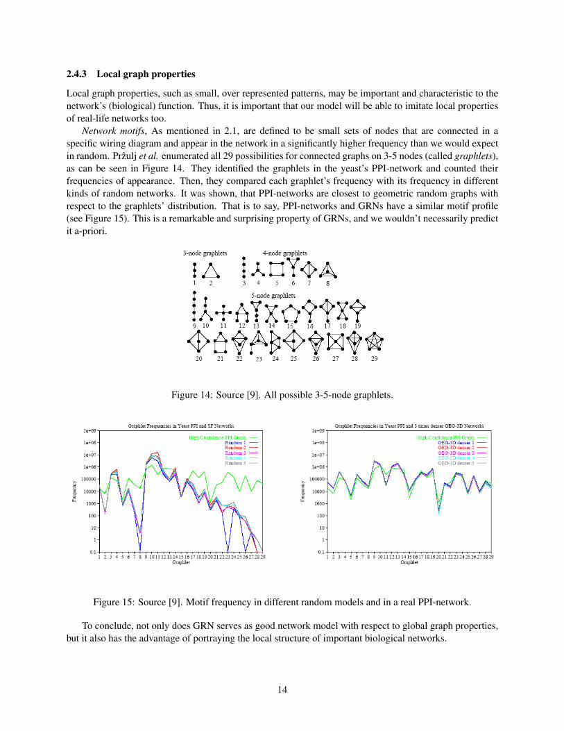
Network motifs, As mentioned in 2.1, are defined to be small sets of nodes that are connected in aspecific wiring diagram and appear in the network in a significantly higher frequency than we would expectin random. Przulj et al. enumerated all 29 possibilities for connected graphs on 3-5 nodes (called graphlets),as can be seen in Figure 14. They identified the graphlets in the yeast’s PPI-network and counted theirfrequencies of appearance. Then, they compared each graphlet’s frequency with its frequency in differentkinds of random networks. It was shown, that PPI-networks are closest to geometric random graphs withrespect to the graphlets’ distribution. That is to say, PPI-networks and GRNs have a similar motif profile(see Figure 15). This is a remarkable and surprising property of GRNs, and we wouldn’t necessarily predictit a-priori.

Figure 14: Source [9]. All possible 3-5-node graphlets.

Figure 15: Source [9]. Motif frequency in different random models and in a real PPI-network.

To conclude, not only does GRN serves as good network model with respect to global graph properties,but it also has the advantage of portraying the local structure of important biological networks.

14

2.5 Exponential Random Graphs

2.5.1 Definition

By now we have seen a variety of random network models, yet each and every one of them lacked one ormore of the properties we would like our network model to have. Is it possible to find a random networkmodel to fulfill all our demands? We will now present a general method for developing such random networkmodel.

According to our observations of real-world networks, we can come up with a set of constrains we wouldlike our network model to satisfy (number of edges/nodes, clustering coefficients, degree distribution, localgraph properties, etc.). All the random network models we have seen so far were generative ones: theydefined a randomized procedure creating a graph to (hopefully) fulfill these constrains. Exponential randomgraphs present a different approach: instead of creating a graph, define a distribution over some ensemble ofgraphs, and sample from this distribution. To make a good model we would like to ensure that the expectedvalue of each property will be equal to its observed value.

We denote our set of observations over m graph properties, {X1, X2, . . . , Xm} as X = {x1, x2, . . . , xm}.Our model contains a large finite set of graphs, G = {G1, G2, . . . , Gn}, and a probability function over theset G,

∑i P (Gi) = 1, such that

∑j P (Gj)Xi(Gj) = xi, where xi is the observed value of property Xi and

Xi(Gj) is the value of property Xi in the graph Gj . Sampling graphs from G according to P ensures thatin expectation we will get a graph which posses all qualities {x1, . . . , xm}.

2.5.2 Choosing the distribution

We have m observations (or constraints) and n graphs. Since usually n is much larger than m, there aremany degrees of freedom in determining a probability function over G that will fulfill our m constraints.That is, there are many distribution functions to choose from. Which one of them should we take?

Out of all choices we pick the probability function that maximizes the entropy. The entropy, S, of adistribution is defined to be:

S(P ) = −∑G

P (G) ln P (G) (19)

This approach is based on the assumption, borrowed from physics, that natural systems tend to maximizetheir entropy. By choosing the probability function with the maximal entropy, we choose the probabilityfunction that assumes as little excessive information as possible.

Another way of looking at it is to think of the following experiment: suppose we have n bins, a binfor each graph in G, and q infinitesimal identical particles of size 1/q each. We throw each of the particlesindependently, with equal probability to fall in each of the bins. The result of such an experiment defines adistribution over G (e.g., if r particles fell into bin i than P (Gi) = r/q). We repeat the experiment until thedistribution we obtain satisfies {x1, . . . , xm}. This is a simple experiment with multinomial distribution. Ifwe calculate which of the valid results it is most likely to obtain in the experiment, we will see that it is theprobability function that has the maximum entropy: The probability to obtain an outcome {k1, k2, . . . , kn},where ki denotes the number of particles that fell into bin i, is:

Pr({k1, k2, . . . , kn}) = W · (1q)q (20)

where

W =q!

k1!k2!...kn!(21)

15

The most probable result is the one which maximizes W . Rather than maximizing W directly we canequivalently maximize any monotonic increasing function of W . We choose to maximize

lnW = lnq!

k1!k2!...km!(22)

= ln q!−n∑

i=1

ln ki! (23)

We take the limit q →∞. Using Stirling’s approximation, we get:

limq→∞

lnW = q ln q −n∑

i=1

ki ln ki

We devide it by q:

ln q −n∑

i=1

ki

qln ki

= ln q −n∑

i=1

P (Gi) ln ki

= ln q −n∑

i=1

P (Gi) ln(qP (Gi))

= ln q −n∑

i=1

P (Gi) ln q −n∑

i=1

P (Gi) ln P (Gi)

=

(1−

n∑i=1

P (Gi)

)ln q −

n∑i=1

P (Gi) ln P (Gi)

= −n∑

i=1

P (Gi) ln P (Gi)

= −∑G

P (G) ln P (G)

= S(P )

Meaning, in order to maximize W , we should maximize the entropy.

2.5.3 The entropy-maximizing distribution

We chose the probability function for our model, P (G), and now we wish to write it explicitly. We seek adistribution P that maximizes S (entropy) while ensuring

∑i P (Gi) = 1 (i.e., P is a probability function

over G) and for each 1 ≤ i ≤ m, E(i) = xi. To do that we apply the Lagrange Multipliers technique. Weget:

∂

∂P (G)

[S + α

(1−

∑G

P (G)

)+∑

i

θi

(xi −

∑G

P (G)Xi(G)

)]= 0 (24)

16

where α and {θi} are Lagrange multipliers. This gives

lnP (G) + 1 + α +∑

i

θiXi(G) = 0 (25)

which yields

P (G) =1Z

exp

(−∑

i

θiXi(G)

)(26)

where Z is a normalization factor.Clearly, Z = e1+α. Since P (G) is a probability function we can also write Z as−(

∑G

∑i θi ·Xi(G)).

Calculating Z analytically is impossible since it requires summing over all the graphs in G (G’s size isenormous). Since we cannot write Z explicitly we have a problem writing P (G) explicitly. In complexmodels the θi’s also cannot be calculated analytically, but they can be estimated using numerical methods.

2.5.4 Sampling

Seemingly we have come to a dead end: we know which distribution we want for our model, and we knowhow to write its equation, but we cannot express it explicitly. However, it turns out that though we cannotcalculate the distribution explicitly, we can sample graphs from G according to this distribution. This isdone using the Markov Chain Monte-Carlo (MCMC) technique. For practical purposes sampling accordingto the desired distribution is sufficient.

2.6 Monte Carlo Markov Chains (MCMC)

Markov chains are useful in a variety of calculation and optimization problems in bioinformatics which atfirst look seem unrelated to the technique. The methods used are described as Markov Chain Monte-Carlo(MCMC) methods. We apply a basic MCMC method called Metropolis, in order to sample according toa distribution without knowing explicitly its values. The idea is to construct a Markov chain on the set ofgraphs G and use the chain’s statistics to estimate the distribution P (G).

2.6.1 Markov chain

We introduce discrete-time finite Markov chains in abstract terms as follows. Consider some finite discreteset S of possible “states”, labeled {E1, E2, . . . , Es}. At each of the unit time points t = 0, 1, 2, 3, . . . , aMarkov chain process occupies one of these states. In each time step t to (t + 1), the process either stays inthe same state or moves to some other state in S according to some well-defined probabilistic rule describedin more detail below. The process is called Markovian, and follows the requirements of a Markov chain if ithas the following distinguishing characteristics:

1. The memoryless property. If at some time t the process is in state Ei, the probability that one timeunit later it is in state Ej depends only on Ei, and not on the past history of the states it was in beforetime t. That is, the current state is all that matters in determining the probabilities for the states thatthe process will occupy in the future.

Pr(Si|Si−1 . . . S1) = Pr(Si|Si−1) (27)

where Si is the state occupied at time i.

17

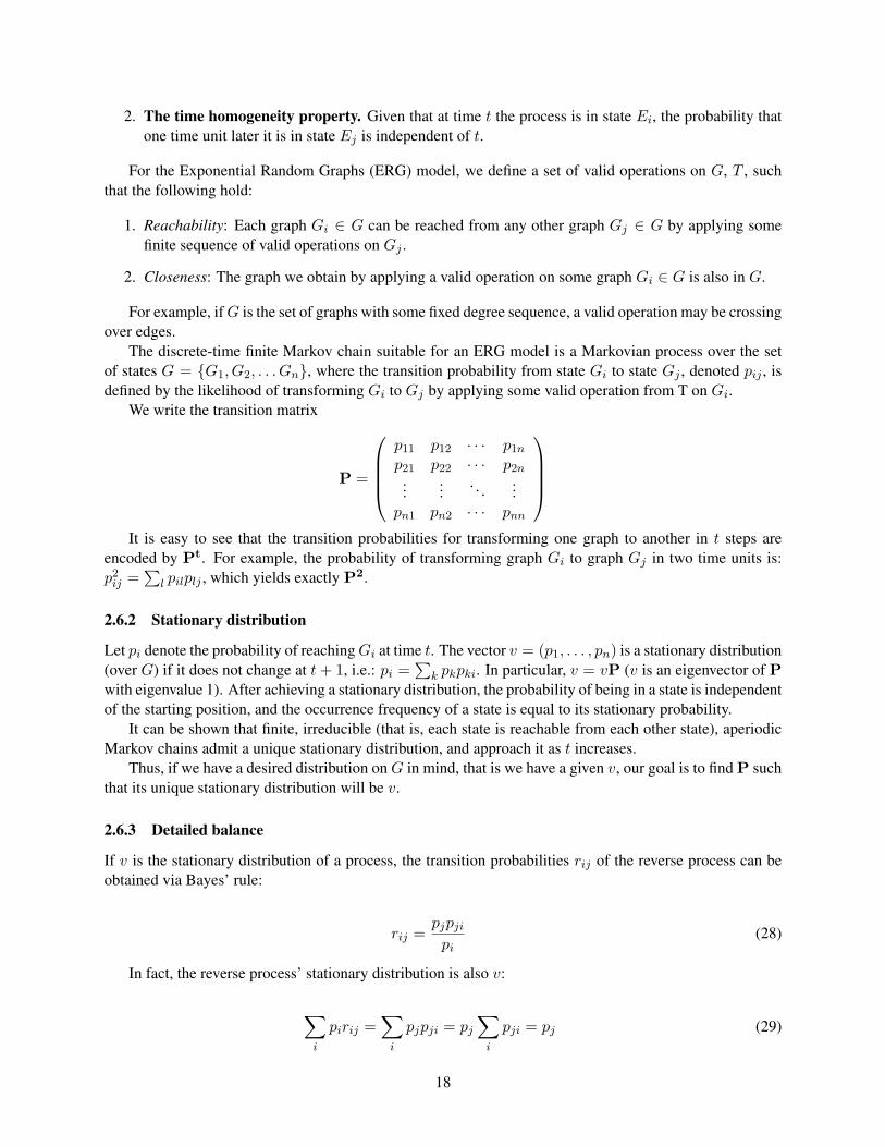
2. The time homogeneity property. Given that at time t the process is in state Ei, the probability thatone time unit later it is in state Ej is independent of t.

For the Exponential Random Graphs (ERG) model, we define a set of valid operations on G, T , suchthat the following hold:

1. Reachability: Each graph Gi ∈ G can be reached from any other graph Gj ∈ G by applying somefinite sequence of valid operations on Gj .

2. Closeness: The graph we obtain by applying a valid operation on some graph Gi ∈ G is also in G.

For example, if G is the set of graphs with some fixed degree sequence, a valid operation may be crossingover edges.

The discrete-time finite Markov chain suitable for an ERG model is a Markovian process over the setof states G = {G1, G2, . . . Gn}, where the transition probability from state Gi to state Gj , denoted pij , isdefined by the likelihood of transforming Gi to Gj by applying some valid operation from T on Gi.

We write the transition matrix

P =

p11 p12 · · · p1n

p21 p22 · · · p2n...

.... . .

...pn1 pn2 · · · pnn

It is easy to see that the transition probabilities for transforming one graph to another in t steps are

encoded by Pt. For example, the probability of transforming graph Gi to graph Gj in two time units is:p2

ij =∑

l pilplj , which yields exactly P2.

2.6.2 Stationary distribution

Let pi denote the probability of reaching Gi at time t. The vector v = (p1, . . . , pn) is a stationary distribution(over G) if it does not change at t + 1, i.e.: pi =

∑k pkpki. In particular, v = vP (v is an eigenvector of P

with eigenvalue 1). After achieving a stationary distribution, the probability of being in a state is independentof the starting position, and the occurrence frequency of a state is equal to its stationary probability.

It can be shown that finite, irreducible (that is, each state is reachable from each other state), aperiodicMarkov chains admit a unique stationary distribution, and approach it as t increases.

Thus, if we have a desired distribution on G in mind, that is we have a given v, our goal is to find P suchthat its unique stationary distribution will be v.

2.6.3 Detailed balance

If v is the stationary distribution of a process, the transition probabilities rij of the reverse process can beobtained via Bayes’ rule:

rij =pjpji

pi(28)

In fact, the reverse process’ stationary distribution is also v:

∑i

pirij =∑

i

pjpji = pj

∑i

pji = pj (29)

18

Suppose that at some time point t, our Markov chain reaches a distribution q = (q1, . . . , qn), whereqi is the probability of occupying Gi at time t, so that for all pairs i, j: qipij = qjpji. This property of(q1, . . . , qn) is called detailed balance. Summing over all i we get:

∑i

qipij =∑

i

qjpji = qj

∑i

pji = qj (30)

That is, for every j, the probability of occupying Gj at time t+1 is equal to the probability of occupyingGj at time t. In other words, q is a stationary distribution of our Markov chain. If our chain is irreducibleand aperiodic, we conclude that a distribution q that satisfies the detailed balance equations is necessarilythe stationary distribution.

The last conclusion is important, since many times we cannot calculate the stationary distribution ofa Markov chain directly, but we do know how to find it via calculating a distribution which satisfies thedetailed balance equations.

A Markov chain is considered reversible if the probability to reach state Si from state Sj is equal to theprobability of reaching Sj from Si. It is easy to see, that a Markov chain has a distribution which satisfiesthe detailed balance equations if and only if it is reversible. i.e., pij = pji.

rij =pjpji

pi=

pipij

pi= pij (31)

Clearly, the reversibility of the Markov chain we construct for an ERG model is determined by thecharacter of the valid operations set, T , and the probability assigned to each operation. Hence, choosing anadequate operation set ensures that the ERG’s Markov chain has a distribution which satisfies the detailedbalance equations.

We wish to sample from the distribution v = (p1, . . . , pn) which is not computable analytically. Ifwe knew how to construct a chain whose transition probabilities satisfy the detailed balance equations whenreaching distribution v, then, since v is the stationary distribution, sampling from this Markov chain through-out a long enough period of time is equivalent to sampling according to the distribution v. In the next sectionit will be shown that it is possible to construct a Markov chain so that its stationary distribution is exactlythe one we are interested in sampling from, P (G).

2.6.4 The Metropolis algorithm

The Metropolis algorithm is a sampling algorithm. It is one of the simplest MCMC methods. The aimof the Metropolis algorithm is to construct an aperiodic irreducible Markov chain having some prescribedstationary distribution. In our case the desired stationary distribution is P (G).

The Metropolis algorithm requires two components:

1. A symmetric proposal mechanism: the probability to move from state Ei to state Ej is equal to theprobability to move from state Ej to state Ei. This can be achieved by defining the set of valid opera-tions, T , to be symmetrical. Formulated using the notations we use for ERG models the requirementis pij = pji.

2. Acceptance of a move with probability min(1, P r(Ej)/Pr(Ei)). In our notation, min(1, P (Gj)/P (Gi))

The Metropolis algorithm defines the sampling distribution (the transition probability over the Markovchain), as follows: the probability of moving to state Ej from state Ei is the product of the transition

19

probability from Ei to Ej and the probability of accepting a move from Ei to Ej . Formulated in our termswe get that the metropolis transition probability is:

q(Gj |Gi) = pij ·min(1, P (Gj)/P (Gi)) (32)

Metropolis has characteristics of a greedy algorithm: if P (Gi) is bigger than P (Gj) accept this movewith probability 1. Otherwise accept the move with some probability related to the ratio between P (Gj)and P (Gi):

Pr(accept move from Gi to Gj) ={

1 P (Gj) > P (Gi)P (Gj)/P (Gi) otherwise

(33)

Claim: Metropolis sampling satisfies detailed balance.Proof:

P (Gi)q(Gj |Gi) = P (Gi) · pij ·min(1, P (Gj)/P (Gi)) (34)

= pij ·min(P (Gi), P (Gj)) = pji ·min(P (Gj), P (Gi)) = P (Gj)q(Gi|Gj)

Recall (2.6.3) that the fact that the probability function P (G) satisfies detailed balance with the transitionfunction, shows it to be the stationary distribution of our Markov chain. That means that if we use theMetropolis transition probability in our Markov chain, after some sufficient time, we will sample graphsfrom G according to the desired distribution P (G).

Note, that in order to write the transition function, q, explicitly we only need to be able to calculateexpressions of the form P (Gi)/P (Gj). Since in these expressions the normalization factor, Z, cancels out,calculating them is easy. Luckily, Monte Carlo algorithms of this type are straightforward to implement andappear to converge quickly allowing us to study quite large graphs.

3 Conclusions

Considering all the models described above, we conclude that no model perfectly fits the networks weobserve in practice. In other words, every model captures only some of the attributes of real networks.We have also seen that statistical methods, such as exponential random graphs, pose an alternative to thegenerative techniques. Nevertheless, generalized random graphs are the most popular in the field, and arecommonly used in the (applied) literature.

References

[1] R. Albert and A. L. Barabasi. Statistical mechanics of complex networks. Reviews of Modern Physics,74:47–97, 2002.

[2] Albert-Laszlo Barabasi and Reka Albert. Emergence of Scaling in Random Networks. Science,286(5439):509–512, 1999.

[3] E. A. Bender and E. R. Canfield. The asymptotic number of labeled graphs with given degree se-quences. J. Comb. Theory, Ser. A, 24(3):296–307, 1978.

[4] P. Erdos and A. Renyi. On the evolution of random graphs. MTA Mat. Kut. Int. K ozl., 5:17–61, 1960.

20

[5] R. Milo, N. Kashtan, S. Itzkovitz, M. E. J. Newman, and U. Alon. On the uniform generation ofrandom graphs with prescribed degree sequences. May 2004.

[6] R. Milo, S. Shen-Orr, S. Itzkovitz, N. Kashtan, D. Chklovskii, and U. Alon. Network motifs: Simplebuilding blocks of complex networks. Science, 298:824–827, 2002.

[7] M. E. J. Newman. The structure and function of complex networks. SIAM Review, 45:167–256, 2003.

[8] N. Przulj. Graph theory analysis of protein-protein interactions. 2005.

[9] N. Przulj, D. G. Corneil, and I. Jurisica. Modeling interactome: Scale free or geometric? arXiv:q-bio.MN/0404017, 2004.

[10] Duncan J. Watts and Steven H. Strogatz. Collective dynamics of ‘small-world’ networks. Nature,393:440–42, 1998.

21