Analysis of Biological Networks:

Network Modules Identi�cation∗

Lecturer: Roded Sharan Scribe: Regina Ring and Constantin Radchenko

Lecture 4, March 25, 2009

In this lecture we complete the discussion of Global Methods of Functional Annotation and present Net-work Modules Identi�cation methods: Protein Complexes Identi�cation (MCODE, NetworkBLAST, Modu-larity and Community Structure in Networks) and Biclustering(SAMBA) and CoIP data analysis(CODEC).

1 Functional Annotation - Global Methods

In the previous lecture we saw several local methods of �nding functions. Similar to local methods, globalmethods are based on the assumption that proteins involved in similar functions are more likely to interact.However, global methods use di�erent strategies for the prediction of protein function and some of them willbe described here.

1.1 Functional �ow

The local methods that we saw in the previous lecture [15, 10] do not consider the global topology of theprotein interaction graphs. Therefore, considering the 2 instances shown in Figure 1, all local methods willproduce the same result for protein a in both instances. These methods ignore information on the numberof independent paths between protein a and the annotated proteins, in addition, these methods treat alldistances equally. The method described in Nabieva et al. [13] is a network �ow, where every protein withknown function is a source of �ow to the other proteins, and the edges are weighted according to theirreliability. The functional �ow algorithm generalized the principle of �guilt by association� to groups ofproteins that may or may not interact with each other physically. A general outline of this algorithm is asfollows:

• Each protein with known function is treated as a source of �ow for that function.

• For each function, �ow spread is simulated by an iterative algorithm using discrete time steps.

• The capacity of an edge is de�ned to be its weight and will represent its reliability.

• The reservoir of a node is the amount of �ow the node can pass to its neighbors. Source nodes havein�nite reservoir; for all others it is initially zero.

• The algorithm is run for several iterations.

• Each iteration a node pushes �ow residing in its reservoir such that:

� Flow is proportional to edge capacities of the node.

� Capacity constraints are satis�ed.

� Flow only spreads from more �lled to less �lled reservoirs.

• Functional score: amount of �ow that entered the protein's reservoir throughout the algorithm.

∗Based on a previous scribes by Udi Ben Porat, Ophir Blieberg, Shaul Karni And Aharon Sharim.

1

Figure 1: Source [13].Two protein interaction graphs that are treated identically by Neighborhood-Countingwith radius 2 when annotating protein a. Dark colored nodes correspond to proteins that are known to takepart in the same process.

1.1.1 The formal algorithm

• R(u) reservoir of u. In�nite for sources; otherwise it is initiated as zero .

• g(u, v) �ow from u to v. Initially, on time 0, there is no �ow on all edges. At each subsequent timestep, the reservoir of each protein is recomputed by considering the amount of �ow that has enteredthe node and the amount that has left:

Rat (u) = Ra

t−1(u) +∑

v:(u,v)∈E

(gat (v, u)− ga

t (u, v)) (1)

At each subsequent time step, the �ow proceeding downhill and satisfying the capacity constraints:

gat (v, u) =

{0 if Ra

t−1(u) < Rat−1(v),

min(wu,v,wu,v∑

(u,y)∈E wu,y) otherwise

(2)

• The algorithm is run for d=6 iterations (enough to propagate �ow from the source to all recipients).

• The �nal functional score for u is the sum of all �ows which entered into the vertex during the wholealgorithm run:

fa(u) =d∑

t=1

∑v:(u,v)∈E

gat (v, u) (3)

1.1.2 Comparison to previous approaches

There are several methods for performance evaluation. One of the methods uses Receiver Operator Charac-teristic (ROC) curves to compare the number of correctly predicted proteins vs number of proteins predictedincorrectly. A protein is considered to be predicted correctly if at least half of the predicted functions arecorrect. An example of such comparison we can see at Figure 2 (Nabieva et al.[13]). It shows that theFunctional Flow algorithm identi�es more true-positives (TPs) over the entire range of false positives (FPs)than either GenMultiCut or Chi-square, using radius 1,2 and 3.

Another method for performance comparison is to show a relation between precision: percentage ofpredictions of the algorithm that are really correct, and recall : percentage of real functions that the algorithm

2

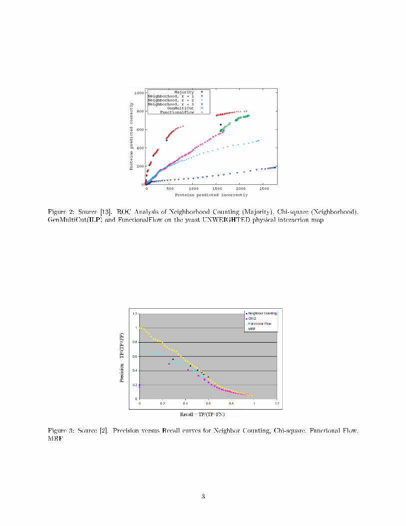
Figure 2: Source [13]. ROC Analysis of Neighborhood Counting (Majority), Chi-square (Neighborhood),GenMultiCut(ILP) and FunctionalFlow on the yeast UNWEIGHTED physical interaction map

Figure 3: Source [2]. Precision versus Recall curves for Neighbor Counting, Chi-square, Functional Flow,MRF

3

Figure 4: Illustration of the basic idea of probabilistic methods. The function of the red node is independentof all the nodes in the graph except its direct neighbors (yellow)

succeeded to predict, like in Figure 3 (Chua et. al. [2]). From this �gure one can assume that the complicatedmethods using global network data (Chi-square, Functional Flow) have lower performance than simplemethods like Neighborhood Counting, whereas the MRF method (which is not explained here) has the bestperformance in comparison to Neighbor Counting, Chi-square and Functional Flow.

1.2 Probabilistic methods

Another approach for predicting functional annotations is using probabilistic modeling.The basic idea of the probabilistic methods is that a node's function is independent of the function of non-

direct neighbors given the function of its direct neighbors. A protein's function depends on its neighbors'function, the neighbors' functions depend on their neighbors and so on. This means that if we label anode in a particular function - it is conditionally independent of all other nodes given its neighbors (Seeillustration in Figure 4). Conditional independence of all other nodes given a vertex's neighbors is calledMarkovian property. In a simpler model a Markov chain is a sequence x1, x2, x3, ... of random variables inwhich the conditional probability distribution of xn+1 on past states (values of previous variables, x1, ..., xn)is a function of xn alone, i.e:

P (xn+1 = an+1|x1 = a1, x2 = a2, ..., xn = an) = P (xn+1 = an+1|xn = an) (4)

In other words, the chain satis�es the Markovian property, in any state it �remembers� only the previousstate. Similarly we can de�ne Markov Random Field (MRF) as an undirected graph in which the verticesrepresent the random variables and the edges re�ect the relation between these random variables. The graphwill also maintain the short memory property (Markovian property). The state of a given vertex xt givenits immediate neighbors states is independent of all the other vertices states, i.e:

P (xt = at|xs = as, s 6= t) = P (xt = at|xs = as, s ∈ Nei(t)) (5)

as Nei(t) is the group of indexes of the t 'th vertex neighbors.In order to �nd protein function we can de�ne a random variables in such a way that each random variable

corresponds to a protein, and its states correspond to certain functional annotations. The joint distributionof the random variables can be shown to factorize over the cliques of the network [1]. Gibbs sampling can beused to infer the unknown functional annotations. Gibbs Sampling is an algorithm for generating a sequenceof samples from the joint distribution of multiple random variables when the distribution is unknown butthe conditional distribution of each variable is known.

1.3 Module based methods

A trivial usage of modules in order to predict gene function will be �guilt by association�. In other words,given a module that some of its proteins are known to have a certain function we can predict that theother proteins of the module also have this function. In the following sections we will describe a number ofalgorithms for automatic module detection.

4

2 Network Modules Identi�cation - Clustering

2.1 Introduction

The main topic of this lecture is the discovery of gene/protein modules in a given network. A module isa set of genes/proteins performing a distinct biological function in an autonomous manner. The genes ina module are characterized by coherent behavior with respect to certain biological property. Examples ofmodules:

• Transcriptional module: a set of co-regulated genes sharing a common function.

• Protein complex : assembly of proteins that build up some cellular machinery; commonly spans a densesub-network of proteins in a protein interaction network.

• Signaling pathway : a chain of interacting proteins propagating a signal in the cell.

The following discussion focuses on �nding protein complexes.

2.2 Clustering

2.2.1 Introduction

The goal of clustering algorithms is to partition the elements (genes) into sets, or clusters, while attemptingto optimize:

• Homogeneity - Elements inside a cluster are highly similar (connected) to each other.

• Separation - Elements from di�erent clusters have low similarity (are sparsely connected) to each other.

In real biology, however, clusters may overlap and need not cover the entire proteome.

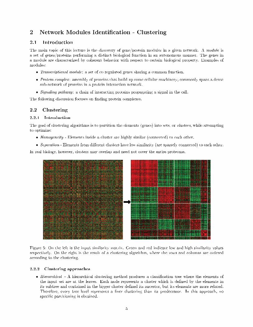
Figure 5: On the left is the input similarity matrix. Green and red indicate low and high similarity valuesrespectively. On the right is the result of a clustering algorithm, where the rows and columns are orderedaccording to the clustering.

2.2.2 Clustering approaches

• Hierarchical - A hierarchical clustering method produces a classi�cation tree where the elements ofthe input set are at the leaves. Each node represents a cluster which is de�ned by the elements inits subtree and contained in the bigger cluster de�ned its ancestor, but its elements are more related.Therefore, every tree level represents a �ner clustering than its predecessor. In this approach, nospeci�c partitioning is obtained.

5

• Non-hierarchical - A non hierarchical method generates a partition of the elements into (generally)non-overlapping groups.

2.2.3 Selected methods

• MCODE: Molecular Complex Detection [3].

• NetworkBLAST[12]

• Modularity and Community Structure in Networks[11].

2.3 MCODE

The MCODE clustering algorithm is a greedy algorithm which detects densely connected regions in largeprotein-protein interaction networks that may represent molecular complexes. The method is based on vertexweighting by local neighborhood density and outward traversal from a locally dense seed protein to isolatethe dense regions according to given parameters[3]. The MCODE algorithm operates in three stages: vertexweighting, complex prediction and postprocessing.

2.3.1 Vertex weighting

For a given graph G(V,E) (|V | number of vetrices and |E| number of edges) we de�ne several terms:

• The open neighborhood of a vertex v ∈ V (G) is de�ned as NG(v) = {u ∈ V (G)|uv ∈ E}, the set of allvertices adjacent to v. The closed neighborhood of a vertex v ∈ V (G) is de�ned as NG[v] = {v}∪NG(v),the set of all vertices adjacent to v including v.

• k−core is a graph of minimal degree k: graph G(V,E) s.t. for all v ∈ V (G), deg(v) ≥ k.

• Highest k-core corresponds to highest k which yields a non-empty graph.

• Density of a graph with no loop is fraction of edges out of all possible vertex pairs: DG = 2|E||V |(|V |−1) .

• The density of the k-core of vertex v is 2nkv(kv−1) where kv is the vertex size of the neighborhood of

vertex v and n is the number of edges in the neighborhood.

The weight of a vertex v ∈ V (G) is de�ned as the density of the highest k-core of its closed neighborhood(the immediate neighborhood density of v including v), multiplied by the corresponding k. This weightingscheme further boosts the weight of densely connected vertices.

2.3.2 Molecular Complex Prediction

The second stage, molecular complex prediction:

• Takes as input the vertex weighted graph

• Seeds a complex with the highest weighted vertex

• Recursively moves outward from the seed vertex, including vertices in the complex whose weight isabove a given threshold w

� w is a given percentage away from the weight of the seed vertex v or vertex weight percentageparameter.

� if a vertex is included, its neighbors are recursively checked in the same manner to see if they arepart of the complex. A vertex is not checked more than once.

• The process stops once no more vertices can be added to the complex based on the given threshold w.

• The process is repeated for the next highest unseen weighted vertex in the network.

In this way, the densest regions of the network are identi�ed. The vertex weight threshold parameter de�nesthe density of the resulting complex. A threshold that is closer to the weight of the seed vertex identi�es asmaller, denser network region around the seed vertex.

6

2.3.3 Postprocessing

The goal of this stage is to �lter or to add proteins in the resulting complexes by certain connectivity criteria.Complexes are �ltered if they do not contain at least a 2-core(graph of minimum degree 2). If the algorithmis run using the 'haircut' option, the resulting complexes are 2-cored, thereby removing the vertices that aresingly connected to the core complex. The algorithm may be run with the '�u�' option, which increases thesize of the complex according to a given '�u�' parameter between 0.0 and 1.0. For every vertex v in thecomplex, its neighbors are added to the complex if they have not yet been seen and if the density of theneighborhood that they create with v is higher than the given '�u�' parameter. Vertices that are added bythe '�u�' parameter are not marked as seen, so there can be overlap among predicted complexes with the'�u�' parameter set.

Resulting complexes from the algorithm are scored and ranked. The complex score is de�ned as theproduct of the density of the complex subgraph and the number of vertices in the complex subgraph. Thisranks larger more dense complexes higher in the results.

MCODE may also be run in a directed mode where a seed vertex is speci�ed as a parameter. In thismode, MCODE only runs once to predict the single complex that the speci�ed seed is a part of. Whenanalyzing complexes in a given network, one would �nd all complexes present (undirected mode) and thenswitch to the directed mode for the complexes of interest. The directed mode allows one to experiment withMCODE parameters to �ne tune the size of the resulting complex according to existing biological knowledgeof the system. In directed mode, MCODE will �rst pre-process the input network to ignore all vertices withhigher vertex weight than the seed vertex. A seed vertex for directed mode should always be the highestdensity vertex among the suspected complex.

2.3.4 MCODE Limitations

There are several limitations in MCODE: the algorithm is heuristic and do not based on a probabilisticmodel. Without using the '�u�' parameter the resulting complexes cannot overlap. Another problem is howto determine the threshold parameters in order to receive good results.

2.4 NetworkBLAST[12]

Opposite to MCODE 2.3 that is completely heuristic approach, the NetworkBLAST method is based onprobability analysis, nevertheless, it still uses some �greedy� heuristic steps (as the problem is NP-hard).

2.4.1 A world of likelihood

Firstly, we are going to de�ne term of Likelihood. For some experimental data, determination of its proba-bilistic model means estimation of the data values distribution, e.g. data D is estimated by distribution thatis de�ned by probabilistic modelM (Θ). So, for probabilistic modelM (Θ) we de�ne likelihood as probabilityto observe our data D.

L (M (Θ)) = P (D|M (Θ)) (6)

So, one of the acceptable approaches to de�ne the parameter Θ, i.e. data distribution, is to maximizethe likelihood of our data, given the probabilistic model M (Θ). Nevertheless, we are going to deal with aslightly di�erent parameter that is called likelihood ratio and is de�ned by Neyman-Pearson as

Λ =L (M1 (Θ))L (M0 (Θ))

(7)

where M0 (Θ) is a default random (null) model and M1 (Θ) is called alternative model and it is morestructured to our data.

So, our purpose is to compare the two models and to conclude which one is more preferential for our dataset. We use this likelihood ratio as a scoring function to assign a score to protein complexes we inferred,i.e. we compare probability of the inferred complexes in the alternative model vs probability of the samecomplex in the random model.

7

2.4.2 Scoring, take I

Now assume that we found proteins complexes (we will show very simple algorithm that �nds such com-plexes), i.e. we found some set of proteins that we expect it to be complex, and we want to give it score.When assigning a score to a complex, in the alternative model, every possible interaction in the subnetworkexists with some high probability p, independently of other protein pairs. This approach to assign probabili-ties is correct due to our assumption that in the complex each node is connected to all other ones. In the nullmodel, every two proteins u, v are connected with probability p (u.v) that depends on their degrees. p (u.v)can be estimated by generating a collection of random networks preserving the degree of every protein andcalculating the fraction of networks in which an interaction between u and v exists. The likelihood ratio ofthe two alternatives for a set of proteins C with a set of interactions E′ is thus

Λ (C) =∏

(u,v)∈E′

p

p(u, v)

∏(u,v)/∈E′

1− p1− p(u, v)

(8)

Pay attention, that if we apply logarithmic function on both sides and set the weight of each edge (u, v)to be log p

p(u,v) > 0 and the weight of each non-edge (u, v) to be log 1−p1−p(u,v) < 0 , we have that the score of

a subgraph is the sum of weights of its vertex pairs.This approach is simpli�ed as model assumes that both edges and not-edged are the same, but we saw

that this is not correct and in previous sections we showed di�erent edge probabilities. Now we want toincorporate edge reliabilities also into our model.

2.4.3 Scoring, take II

Let's treat interactions between vertices in our model not as real, but rather as noisy observations, and de�neOu,v as set of such observations on interactions between u, v. Now likelihood ratio will be represented as

Λ (C) =∏

(u,v)∈V ′×V ′

Pr (Ou,v |MC)Pr (Ou,v |MN )

(9)

where MC is alternative model of complexes and MN is null model. Given that in model M the pro-tein pair u, v interacts with probability Pr (Ou,v | Tu,v,M) and does not interact with Pr (Ou,v | Fu,v,M),likelihood ratio is de�ned as

Λ (C) =∏

(u,v)∈V ′×V ′

p · Pr (Ou,v | Tu,v,MC) + (1− p) · Pr (Ou,v | Fu,v,MC)p (u, v) · Pr (Ou,v | Tu,v,MN ) + (1− p (u, v)) · Pr (Ou,v | Fu,v,MN )

(10)

According to Bayes rule, Pr (O | T,M) = Pr (T,M | O) Pr(O)Pr(T,M) where Pr (T,M | O) can be calculated

from observations on model M and Pr (Tu,v,M) is an apriori knowledge if edge between u, v exists in modelM. For example if we have 20000 true PPI, so Pr (Tu,v) = 20000

(60002 )≈

2000060002 . The only unknown parameter is

Pr (O), but as we use fraction, it is dropped.

2.4.4 Search algorithm

In order to calculate the score of the complex, we still need to �nd it before, and here we use some �greedy�algorithm. Starting from all the �heaviest� pairs or triangles in graph as seed, try in �greedy� manner to adda new vertex, such that it increases complex score, or remove a vertex, such that removal also increases thecomplex score. We continue these steps until some local maximum is reached, i.e. found a local complexthat is quite �good� and cannot be improved through local changes (adding/removing of a single protein).The main catch is that the algorithm starts from many similar seeds, so it may �nally get similar complexes.To avoid this, the �nal stage of the algorithm comprises �ltering of the overlapping complexes: calculatesintersection between complexes and drops the one with smaller score. In fact, we leave complexes with not toolarge intersections, e.g. no more than half of complex size. Such an approach for complexes �ltering exposesone of the algorithm's drawbacks: in real world we can, obviously, �nd complexes pairs with overlappingover 90% between them, but the algorithm �lters such complexes and keeps only one of them.

8

Figure 6: The vertices in many networks fall naturally into groups or communities, sets of vertices (shaded)within which there are many edges, with only a smaller number of edges between vertices of di�erent groups.

2.5 Modularity and Community Structure in Networks[11]

The previous approach NetworkBLAST (2.4) overcomes most of MCODE(2.3) drawbacks, but this algorithmstill works locally.

Now consider another way that de�nitely has its own advantages, like global view on the system, but ithas greater complexity and also prevents from clusters to be overlapped, that, usually, does not happen innature.

2.5.1 Modularity of a division

Many real-world networks including social networks, computer networks, and metabolic and regulatorynetworks, are found to divide naturally into communities or modules. The problem of detecting and charac-terizing this community structure is one of the outstanding issues in the study of networked systems. We willdiscuss an approach that optimizes the quality function known as ``modularity'' over the possible divisionsof a network. We will also show that the modularity can be expressed in terms of the eigenvectors of acharacteristic matrix for the network, which is called modularity matrix, and that this expression leads tocommunity detection algorithm.

2.5.2 Division into two groups

Suppose then that we are given, or discover, the structure of some network and that we want to determinewhether there exists any natural division of its vertices into non overlapping groups or communities, wherethese communities may be of any size.

Let us approach this question in stages and focus initially on the problem of whether any good division ofthe network exists into just two communities. The problem is that simply counting edges is not a good wayto quantify the intuitive concept of community structure. A good division of a network into communities isnot merely one in which there are few edges between communities; it is one in which there are fewer thanexpected edges between communities. So we are looking not for cases that the number of edges betweentwo groups is expected on basis of random chance, but rather for ones that the number of edges within thegroups is signi�cantly more than we expect by chance.

This idea, that true community structure in a network corresponds to a statistically surprising arrange-ment of edges, can be quanti�ed by using the measure known as modularity [14]. The modularity is, upto a multiplicative constant, the number of edges falling within groups minus the expected number in anequivalent network with edges placed at random. If community sizes are unconstrained then we are, forinstance, at liberty to select the trivial division of the network that puts all of the vertices in one of our

9

two groups and none in the other, which guarantees we will have zero intergroup edges and our modularityparameter will be zero too. Clearly, this division does not tell us anything of any worth.

Suppose our network contains n vertices. For a particular division of the network into two groups letsi = 1 if vertex i belongs to group 1 and si = −1 if it belongs to group 2. And let the number of edgesbetween vertices i and j be Aij , which will normally be 0 or 1, although larger values are possible in networkswhere multiple edges are allowed. (The quantities Aij are the elements of the so-called adjacency matrix.)At the same time, the expected number of edges between vertices i and j if edges are placed at random iskikj

M , where ki and kj are the degrees of the vertices and M =∑ki = 2|E| is the total number of edges

degrees in the network. Thus the modularity Q is given by the sum of Aij − ki ∗ kj/M over all pairs ofvertices i, j that fall in the same group.

Observing that the quantity 12 (sisj + 1) is 1 if i and j are in the same group and 0 otherwise, we can

then express the modularity as

Q =∑

(Aij − ki ∗ kj/M | i, j in the same group) = (11)

= 12

∑ij

(Aij − kikj

M

)(sisj + 1) = 1

2

∑ij

(Ai,j − ki∗kj

M

)sisj

where the second equality follows from the observation that M =∑

i ki =∑

ij Aij .Eq. 11 can conveniently be written in matrix form as

Q =12sTBs (12)

where s is the column vector whose elements are the si and we have de�ned a real symmetric matrix Bwith elements

Bij = Aij −kikj

M(13)

which we call the modularity matrix. Observing this matrix properties, it is easy to note that the elementsof each of its rows and columns sum to zero, so that it always has an eigenvector (1,1,1, . . .) with eigenvaluezero. Matrix B is also symmetric, so it is diagnosable, i.e. it has real eigenvalues.

Given Eq. 12, we proceed by writing s as a linear combination of the normalized eigenvectors ui of B sothat s =

∑ni=1 aiui with ai = uT

i � s. Then we �nd

Q =12sTBs =

12

∑i

(aiu

Ti

)B∑

j

(ajuj) =12

∑i

(aiu

Ti

)∑j

aj (Buj) =12

∑i

(aiu

Ti

)∑j

aj (βjuj) = (14)

= 12

∑i

∑j aiu

Ti ajβjuj = 1

2

∑i a

2iβi

where βi is the eigenvalue of B corresponding to eigenvector ui. Note that ∀i 6= j : uTi uj = 0 as ui are

orthonormal basis of B.Assume that the eigenvalues are labeled in decreasing order, β1 ≥ β2 ≥ . . . ≥ βn. We want to maximize

the modularity by choosing an appropriate division of the network, or equivalently by choosing the value ofthe index vector s. This means choosing s so as to concentrate as much weight as possible in terms of thesum in Eq. 14 involving the largest (most positive) eigenvalues. If there were no other constraints on ourchoice of s (apart from normalization), this would be an easy task: we would simply chose s proportionalto the eigenvector u1. This places all of the weight in the term involving the largest eigenvalue β1, the otherterms being automatically zero, because the eigenvectors are orthogonal.

Unfortunately, there is another constraint on the problem imposed by the restriction of the elements ofs to the values ±1, which means s cannot normally be chosen parallel to u1. Let us do our best, however,and make it as close to parallel as possible, which is equivalent to maximizing the dot product uT

1 � s. It isstraightforward to see that the maximum is achieved by setting si = 1 if the corresponding element of ui ispositive and si = −1 otherwise. In other words, all vertices whose corresponding elements are positive goin one group and all of the rest in the other. This then gives us the algorithm for dividing the network: we

10

compute the leading eigenvector of the modularity matrix and divide the vertices into two groups accordingto the signs of the elements in this vector.

We immediately notice some satisfying features of this method. First, as has been made clear, it workseven though the sizes of the communities are not speci�ed. Unlike conventional partitioning methods thatminimize the number of betweengroup edges, there is no need to constrain the group sizes or arti�cially forbidthe trivial solution with all vertices in a single group. There is an eigenvector (1,1,1, . . .) correspondingto such a trivial solution, but its eigenvalue is zero. All other eigenvectors are orthogonal to this one andhence must possess both positive and negative elements. Thus, as long as there is any positive eigenvaluethis method will not put all vertices in the same group.

It is, however, possible for there to be no positive eigenvalues of the modularity matrix. In this case theleading eigenvector is the vector (1,1,1, . . .) corresponding to all vertices in a single group together. Butthis is precisely the correct result: the algorithm is in this case telling us that there is no division of thenetwork that results in positive modularity, as can immediately be seen from Eq. 14, because all terms inthe sum will be zero or negative. The modularity of the undivided network is zero, which is the best thatcan be achieved. This is an important feature of the algorithm. The algorithm has the ability not only todivide networks e�ectively, but also to refuse to divide them when no good division exists. The networks inthis latter case will be called indivisible. That is, a network is indivisible if the modularity matrix has nopositive eigenvalues.

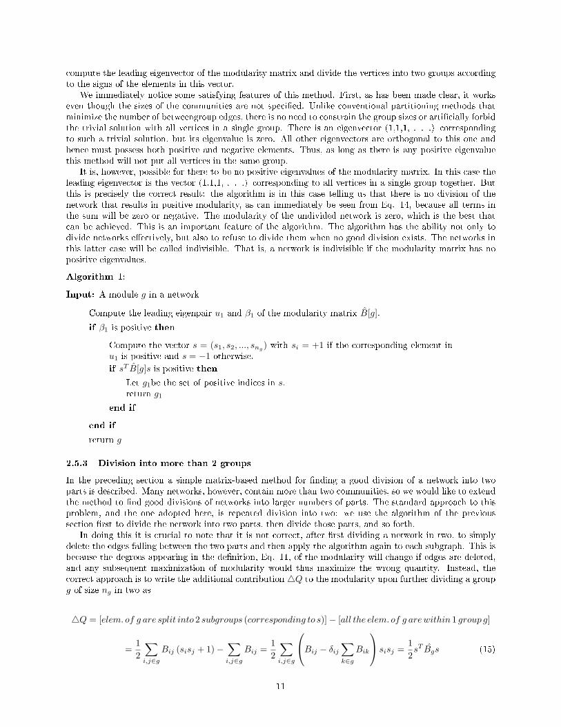
Algorithm 1:

Input: A module g in a network

Compute the leading eigenpair u1 and β1 of the modularity matrix B̂[g].

if β1 is positive then

Compute the vector s = (s1, s2, ..., sng) with si = +1 if the corresponding element in

u1 is positive and s = −1 otherwise.

if sT B̂[g]s is positive then

Let g1be the set of positive indices in s.return g1

end if

end if

return g

2.5.3 Division into more than 2 groups

In the preceding section a simple matrix-based method for �nding a good division of a network into twoparts is described. Many networks, however, contain more than two communities, so we would like to extendthe method to �nd good divisions of networks into larger numbers of parts. The standard approach to thisproblem, and the one adopted here, is repeated division into two: we use the algorithm of the previoussection �rst to divide the network into two parts, then divide those parts, and so forth.

In doing this it is crucial to note that it is not correct, after �rst dividing a network in two, to simplydelete the edges falling between the two parts and then apply the algorithm again to each subgraph. This isbecause the degrees appearing in the de�nition, Eq. 11, of the modularity will change if edges are deleted,and any subsequent maximization of modularity would thus maximize the wrong quantity. Instead, thecorrect approach is to write the additional contribution 4Q to the modularity upon further dividing a groupg of size ng in two as

4Q = [elem. of g are split into 2 subgroups (corresponding to s)]− [all the elem. of g arewithin 1 group g]

=12

∑i,j∈g

Bij (sisj + 1)−∑i,j∈g

Bij =12

∑i,j∈g

Bij − δij∑k∈g

Bik

sisj =12sT B̂gs (15)

11

where δij is 1 for i = j and 0 otherwise, we have made use the fact that s2i = 1, and B̂g is the ng × ng

matrix with elements indexed by the labels i,j of vertices within group g and having values

B̂(g)ij = B(g)ij − δij∑k∈g

Bik = B(g)ij − δijf(g)i (16)

Because Eq. 15 has the same form as Eq. 12 we can now apply the approach to this generalized modularitymatrix, just as before, to maximize 4Q. Note that the rows and columns of Bg still sum to zero and that4Q is correctly zero if group g is undivided. Note also that for a complete network Eq. 16 reduces to theprevious de�nition of the modularity matrix, Eq. 13, because

∑k Bik is zero in that case.

In repeatedly subdividing the network, an important question we need to address is at what point to haltthe subdivision process. A nice feature of this method is that it provides a clear answer to this question: ifthere exists no division of a subgraph that will increase the modularity of the network, or equivalently thatgives a positive value for 4Q, then there is nothing to be gained by dividing the subgraph and it shouldbe left alone; it is indivisible in the sense of the previous section. This happens when there are no positiveeigenvalues to the matrix Bg, and thus the leading eigenvalue provides a simple check for the terminationof the subdivision process: if the leading eigenvalue is zero, which is the smallest value it can take, then thesubgraph is indivisible.

Thus the algorithm is as follows. We construct the modularity matrix, (Eq. 13), for the network and �ndits leading (most positive) eigenvalue and the corresponding eigenvector. We divide the network into twoparts according to the signs of the elements of this vector, and then repeat the process for each of the parts,using the generalized modularity matrix, (Eq. 16). If at any stage we �nd that a proposed split makes a zeroor negative contribution to the total modularity, we leave the corresponding subgraph undivided. When theentire network has been decomposed into indivisible subgraphs in this way, the algorithm ends.

Algorithm 2:

Input: A network with n vertices, n > 1

P ← {{1, 2, .., n}}Mark the single group in P as divisible

while there are divisible group in P do

g ←a divisible group in P

g1 ←the return value of Algorithm 1 on the module g

if |g1| = 0 or |g1| = |g| thenMark gi as indivisible

else

g2 ← g\g1P = P\{g} ∪ {g1, g2}for i = 1 to 2 do

if |gi| = 1 thenMark gi as indivisible

else

Mark gi as divisible

end if

end for

end if

end while

12

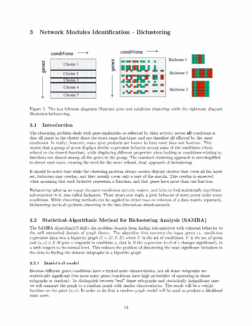
3 Network Modules Identi�cation - Biclustering

Figure 7: The two leftmost diagrams illustrate gene and condition clustering while the rightmost diagramillustrates biclustering.

3.1 Introduction

The clustering problem deals with gene similarities as re�ected by their activity across all conditions isthat all genes in the cluster share the exact same functions, and are therefore all e�ected by the sameconditions. In reality, however, many gene products are known to have more than one function. Thismeans that a group of genes displays similar expression behavior across some of the conditions (thoserelated to the shared function), while displaying di�erent properties when looking at conditions relating tofunctions not shared among all the genes in the group. The standard clustering approach is oversimpli�edto detect such cases, creating the need for the more re�ned, local, approach of biclustering.

It should be noted that while the clustering problem always creates disjoint clusters that cover all the inputset, biclusters may overlap, and they usually cover only a part of the matrix. This overlap is expectedwhen assuming that each bicluster represents a function, and that genes have more than one function.

Biclustering takes as an input the same conditions activity matrix, and tries to �nd statistically signi�cantsub-matrices in it, also called biclusters. These structures imply a joint behavior of some genes under someconditions. While clustering methods can be applied to either rows or columns of a data matrix separately,biclustering methods perform clustering in the two dimensions simultaneously.

3.2 Statistical-Algorithmic Method for Biclustering Analysis (SAMBA)

The SAMBA algorithm[17] shifts the problem domain from �nding sub-matrices with coherent behavior tothe well researched domain of graph theory. The algorithm �rst converts the input genes vs. conditionsexpression data into a bipartite graph G = (U, V,E) where U is the set of conditions, V is the set of genesand (u, v) ∈ E i� gene v responds in condition u, that is, if the expression level of v changes signi�cantly inu with respect to its normal level. This reduces the problem of discovering the most signi�cant biclusters inthe data to �nding the densest subgraphs in a bipartite graph

3.2.1 Statistical model

Because di�erent genes/conditions have a typical noise characteristics, not all dense subgraphs arestatistically signi�cant (the more noisy genes/conditions have high probability of appearing in densesubgraphs at random). To distinguish between �real� dense sub-graphs and statistically insigni�cant oneswe will compare the graph to a random graph with similar characteristics. The result will be a weightfunction on the pairs (u, v). In order to do that a random graph model will be used to produce a likelihoodratio score.

13

Figure 8: Illustration of biclustering approach: �nding high similarity submatrices and dense subgraphs

Random graph model. The null hypothesis model, or random graph mode, assumes that each vertexpair (u, v) forms an edge with probability p(u, v), independently of all other edges. p(u, v) is de�ned to bethe probability of observing an edge (u, v) in a random degree-preserving bipartite graph. p(u, v) is well

approximated by dudvm , where du is the degree of U , dv is the degree of V , and m is the total number of

edges.

Bicluster model. The alternative hypothesis model, or bicluster model, assumes that each edge of abicluster appears with a constant high probability pc.

Likelihood ratio score. The likelihood ratio score L of a sub-graph B = (U ′, V ′, E′) is

L(B) =∏

(u,v)∈E′

pc

p(u, v)

∏u,v/∈E′

1− pc

1− p(u, v)(17)

logL(B) =∑

(u,v)∈E′

logPc

p(u, v)+

∑(u,v)/∈E′

log1− Pc

1− p(u, v)(18)

Setting the weights of the edges to log pc

p(u,v) and the non edges to log 1−pc

1−p(u,v) will result in the score of

B being simply the sum of weights of its edges and non-edges.

3.2.2 Finding the heaviest biclique in a bipartite graph

Theorem 1 Finding the heaviest biclique in a bipartite graph is NP-hard

Proof: This is shown by reduction from CLIQUE. Given a graph G = (V,E) transform it to G′ = (V, V, V ×V,w) such that w(u, v) = 0 for each original edge (u, v) and w(u, v) = −|V |2 for each non-edge, andw(v, v) = 1. If the larges clique is of size k in the original graph there is a biclique of weight k in thebipartite graph. There is no heavier biclique because this will result in a larger click in the original graph aswill be shown next.

If the heaviest biclique in the bipartite graph is k for some k > 0 there is a clique of size k in the originalgraph, this is because there is clearly no edge that was not in the original graph in the biclique because thiswill produce k < 0, hence, the same group of vertices is a clique in the original graph.

14

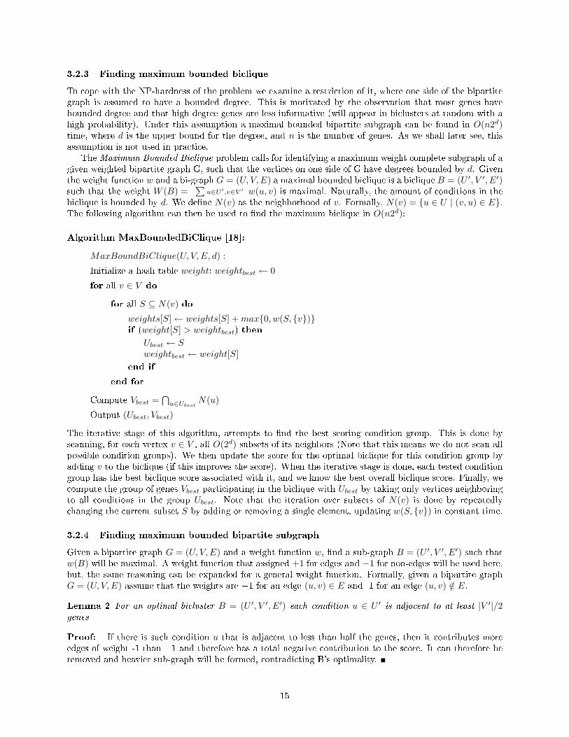
3.2.3 Finding maximum bounded biclique

To cope with the NP-hardness of the problem we examine a restriction of it, where one side of the bipartitegraph is assumed to have a bounded degree. This is motivated by the observation that most genes havebounded degree and that high degree genes are less informative (will appear in biclusters at random with ahigh probability). Under this assumption a maximal bounded bipartite subgraph can be found in O(n2d)time, where d is the upper bound for the degree, and n is the number of genes. As we shall later see, thisassumption is not used in practice.

The Maximum Bounded Biclique problem calls for identifying a maximum weight complete subgraph of agiven weighted bipartite graph G, such that the vertices on one side of G have degrees bounded by d. Giventhe weight function w and a bi-graph G = (U, V,E) a maximal bounded biclique is a biclique B = (U ′, V ′, E′)such that the weight W (B) =

∑u∈U ′,v∈V ′ w(u, v) is maximal. Naturally, the amount of conditions in the

biclique is bounded by d. We de�ne N(v) as the neighborhood of v. Formally, N(v) = {u ∈ U | (v, u) ∈ E}.The following algorithm can then be used to �nd the maximum biclique in O(n2d):

Algorithm MaxBoundedBiClique [18]:

MaxBoundBiClique(U, V,E, d) :

Initialize a hash table weight; weightbest ← 0

for all v ∈ V do

for all S ⊆ N(v) do

weights[S]← weights[S] +max{0, w(S, {v})}if (weight[S] > weightbest) then

Ubest ← Sweightbest ← weight[S]

end if

end for

Compute Vbest =⋂

u∈UbestN(u)

Output (Ubest, Vbest)

The iterative stage of this algorithm, attempts to �nd the best scoring condition group. This is done byscanning, for each vertex v ∈ V , all O(2d) subsets of its neighbors (Note that this means we do not scan allpossible condition groups). We then update the score for the optimal biclique for this condition group byadding v to the biclique (if this improves the score). When the iterative stage is done, each tested conditiongroup has the best biclique score associated with it, and we know the best overall biclique score. Finally, wecompute the group of genes Vbest participating in the biclique with Ubest by taking only vertices neighboringto all conditions in the group Ubest. Note that the iteration over subsets of N(v) is done by repeatedlychanging the current subset S by adding or removing a single element, updating w(S, {v}) in constant time.

3.2.4 Finding maximum bounded bipartite subgraph

Given a bipartite graph G = (U, V,E) and a weight function w, �nd a sub-graph B = (U ′, V ′, E′) such thatw(B) will be maximal. A weight function that assigned +1 for edges and −1 for non-edges will be used here,but, the same reasoning can be expanded for a general weight function. Formally, given a bipartite graphG = (U, V,E) assume that the weights are +1 for an edge (u, v) ∈ E and -1 for an edge (u, v) /∈ E.

Lemma 2 For an optimal bicluster B = (U ′, V ′, E′) each condition u ∈ U ′ is adjacent to at least |V ′|/2genes

Proof: If there is such condition u that is adjacent to less than half the genes, then it contributes moreedges of weight -1 than +1 and therefore has a total negative contribution to the score. It can therefore beremoved and heavier sub-graph will be formed, contradicting B's optimality.

15

Lemma 3 For an optimal bicluster B = (U ′, V ′, E′) each gene v ∈ V ′ is adjacent to at least |U ′|/2 condi-tions.

Proof: The same argument as the proof of the previous Lemma.

Lemma 4 For an optimal bicluster B = (U ′, V ′, E′), |U ′| ≤ 2d

Proof: This is an immediate result of the previous Lemma: If each gene is adjacent to at least |U ′|/2conditions and each gene has a bounded neighborhood of d conditions then |U ′| ≤ 2d.

Lemma 5 For any subset X ⊆ U ′ there exist a gene v ∈ V ′ such that v is adjacent to at least |X|/2 membersof X.

Proof: Assume X such that each gene v ∈ V ′ is connected only to < |X|/2 members of X. This leads tothe conclusion that U ′\X induces a heavier bicluster than U ′ because each gene contributes a negative scoreto X.

Corollary 1 For an optimal bicluster B = (U ′, V ′, E′), U ′ can be covered with at most log(2d) sets eachcontained in the neighborhood of some v ∈ V ′. This allows an O((n2d)log(2d)) algorithm that can be gener-alized to produce k heaviest biclusters by storing the k heaviest in a heap (and adding a multiplicative factorof log(k)).

3.2.5 The SAMBA Algorithm

Although the algorithm described above is polynomial in n, it is still infeasible with today's computationalpower, due to the fact that d is too large. The SAMBA algorithm attempts to address this problem.

SAMBA proceeds in three phases. First, the model bipartite graph is formed and the weights of vertexpairs are computed. Second, several heavy subgraphs are sought around each vertex of the graph. This isdone by starting with good seeds around the vertex and expanding them using local search. The seeds arefound using the hashing technique of the MaxBoundedBiClique algorithm, for all subsets of neighborsof size 4-6 (e�ectively restricting the algorithm complexity). The local improvement procedure iterativelyapplies the best modi�cation to the current bicluster (addition or deletion of a single vertex) until no scoreimprovement is possible.

To avoid similar biclusters whose vertex sets di�er only slightly, a �nal step greedily �lters similar biclus-ters with more than some threshold overlap (usually 20%). The following summarizes the second phase:

1. Find heavy bicliques using algorithm 3.2.3, while restricting to 4-6 neighbors of each gene.

2. Greedy expansion of heaviest bicliques to contain each gene/condition.

3. �lter overlapping biclusters, this is done to avoid similar biclusters whose vertex set di�er only slightly.

3.3 Results obtained with SAMBA

3.3.1 Quality Evaluation when a classi�cation of the genes or conditions is known

The quality of a bicluster solution is determined using a given classi�cation of the conditions or genes asfollows: suppose prior knowledge partitions the m conditions into k classes, C1, ...., Ck . Let B be a biclusterwith b conditions, out of which bj belong to class Cj . The p-value of B, assuming its most signi�cant classis Ci, is calculated as

P (B) =∑

bi≤k≤b

(|Ci|k

)(m− |Ci|b− k

)(mb

) (19)

16

Hence, the p-value measures the probability of obtaining at least bi elements from the class in a randomset of size b (This is also known as a hypergeometric score).

The main tool in evaluating biclustering results using prior biological knowledge is a correspondenceplot. The plot depicts the distribution of p-values of the produced biclusters, using for evaluation a knownclassi�cation of conditions or a given gene annotation. The plot is generated as follows: For each value of pthe plot presents the fraction of biclusters whose p-value is at most p out of the top biclusters. One shouldnote that high quality biclusters can also identify phenomena that are not covered by the given classi�cation.This, theoretically, can result in a biologically �true� bicluster which seems to have a random overlap withknown annotations. Nevertheless, it is expected that a large fraction of the biclusters will conform to theknown classi�cation.

3.3.2 Comparative Analysis

Tanay et al. applied SAMBA to a dataset that contained the expression levels of 4,026 genes over 96 humantissue samples, which are classi�ed into 9 classes of lymphoma and normal ones [17]. The authors comparedtheir performance to:

1. Cheng and Church's algorithm on the lymphoma dataset [20].

2. Random annotation of the 96 samples (preserving class sizes).

Correspondence plots for the biclusters are shown in the next �gure. The plots demonstrate that the biclustersgenerated by SAMBA are much more statistically signi�cant than those obtained with the Cheng-Churchalgorithm.

Figure 9: Source: [17]. Correspondence plots for SAMBA, the algorithm of Cheng and Church (2000), andrandom biclusters.

3.3.3 Combined Yeast Dataset

Modern experimental techniques in biology collect massive amounts of information on the behavior andinteraction of thousands of genes and proteins across diverse conditions. These techniques are used tointerrogate complex biological systems. It is impossible to fully characterize such complex cellular systemsby focusing completely on a single control mechanism, as measured by a single experimental technique. Togain deeper understanding of the systems, it is appropriate to analyze heterogeneous data sources in a truly

17

integrated fashion and shape the analysis results into one body of knowledge. Tanay et al. [16] appliedSAMBA to a diverse sources of biological information from yeast:

• 1,000 expression pro�les, representing 70 sets of conditions from 27 di�erent publications.

• 110 transcription factor binding location pro�les [6].

• 30 growth pro�les [4].

• 1,031 protein interactions [8].

• 4,177 complex interactions and [5].

• 1,175 known interactions from the MIPS (Munich Information center for Protein Sequences) database[7].

An extensive collection of identi�ed modules can improve our understanding of speci�c biological processes.The authors used transcription factor binding pro�les and their correspondence to modules to create adetailed representation of the yeast transcriptional program. They have also automatically generated morethan 800 function predictions for uncharacterized yeast genes and veri�ed some of them experimentally.

3.3.4 Quality Evaluation when the classi�cation is unknown

The statistical signi�cance of the modules was validated by performing a randomized control test (see Figure[18]). SAMBA was applied to real and shu�ed data sets and the distributions of the module were compared:Randomly shu�ed graphs were used to test the statistical signi�cance of the module: Random shu�es of theoriginal graph G were obtained by repeatedly selecting two random edges and crossing them (i.e., replacingedges (g1, p1) and (g2, p2) by (g1, p2) and (g2, p1)), provided that the latter two edges were not alreadyin the graph. This process preserves all of the degrees in the graph. Because the graph includes edgeswith di�erent probabilities, only pairs of edges with nearly identical probabilities were crossed the expectednumber of crosses for each edge was 10. For each module size (size is de�ned as the size of its gene set) thedistribution of the scores was computed. The 90%, 80%, and 50% percentiles for true modules and the 95%,90% and 50% percentiles for modules in randomized data were plotted. The score distribution was computedon the largest 300 modules not exceeding the given size. It is evident that the scores of a large fraction ofthe modules detected in the original data exceed the maximal random score. For each module size the valueof the random 95 percentile was used as a threshold for true module acceptance. The graph also shows thatmodules with 40-70 genes carry a particularly high information content. Indeed, many biological processesin yeast consist of several dozens of interacting proteins or co-regulated genes.

18

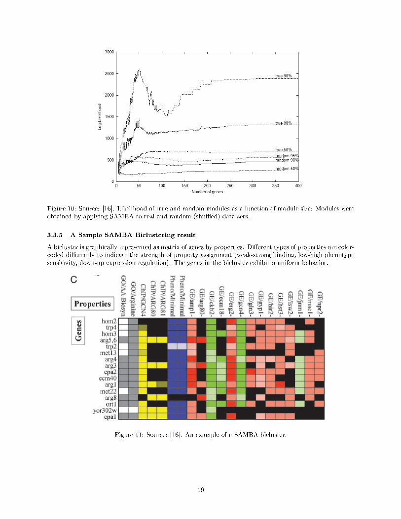
Figure 10: Source: [16]. Likelihood of true and random modules as a function of module size: Modules wereobtained by applying SAMBA to real and random (shu�ed) data sets.

3.3.5 A Sample SAMBA Biclustering result

A bicluster is graphically represented as matrix of genes by properties. Di�erent types of properties are color-coded di�erently to indicate the strength of property assignment (weak-strong binding, low-high phenotypesensitivity, down-up expression regulation). The genes in the bicluster exhibit a uniform behavior.

Figure 11: Source: [16]. An example of a SAMBA bicluster.

19

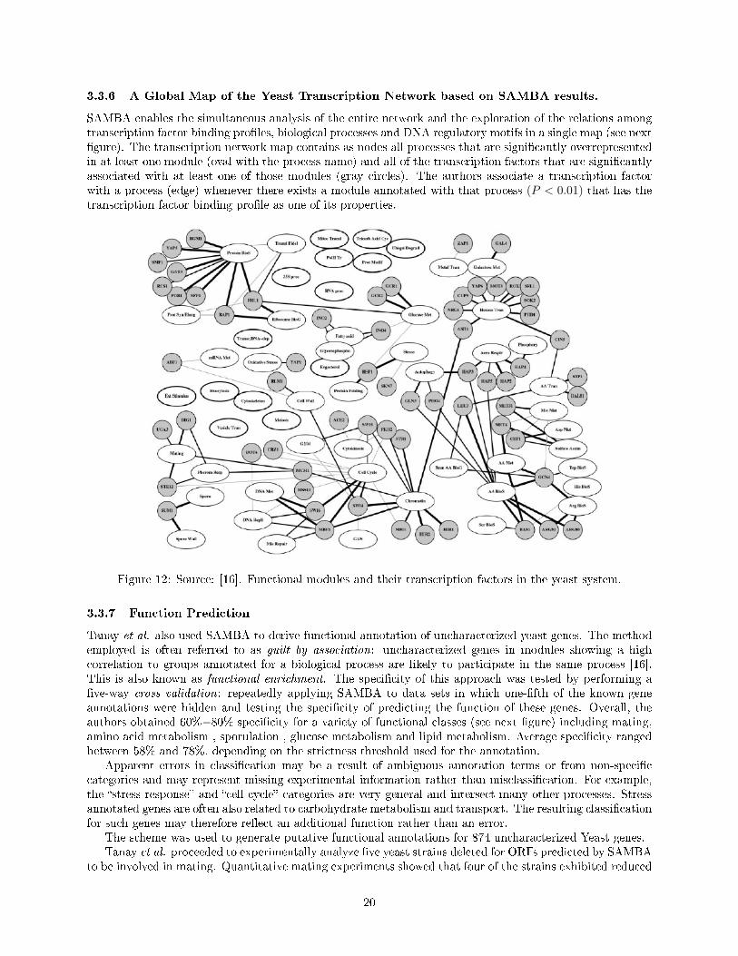
3.3.6 A Global Map of the Yeast Transcription Network based on SAMBA results.

SAMBA enables the simultaneous analysis of the entire network and the exploration of the relations amongtranscription factor binding pro�les, biological processes and DNA regulatory motifs in a single map (see next�gure). The transcription network map contains as nodes all processes that are signi�cantly overrepresentedin at least one module (oval with the process name) and all of the transcription factors that are signi�cantlyassociated with at least one of those modules (gray circles). The authors associate a transcription factorwith a process (edge) whenever there exists a module annotated with that process (P < 0.01) that has thetranscription factor binding pro�le as one of its properties.

Figure 12: Source: [16]. Functional modules and their transcription factors in the yeast system.

3.3.7 Function Prediction

Tanay et al. also used SAMBA to derive functional annotation of uncharacterized yeast genes. The methodemployed is often referred to as guilt by association: uncharacterized genes in modules showing a highcorrelation to groups annotated for a biological process are likely to participate in the same process [16].This is also known as functional enrichment. The speci�city of this approach was tested by performing a�ve-way cross validation: repeatedly applying SAMBA to data sets in which one-�fth of the known geneannotations were hidden and testing the speci�city of predicting the function of these genes. Overall, theauthors obtained 60%−80% speci�city for a variety of functional classes (see next �gure) including mating,amino acid metabolism , sporulation , glucose metabolism and lipid metabolism. Average speci�city rangedbetween 58% and 78%, depending on the strictness threshold used for the annotation.

Apparent errors in classi�cation may be a result of ambiguous annotation terms or from non-speci�ccategories and may represent missing experimental information rather than misclassi�cation. For example,the �stress response� and �cell cycle� categories are very general and intersect many other processes. Stressannotated genes are often also related to carbohydrate metabolism and transport. The resulting classi�cationfor such genes may therefore re�ect an additional function rather than an error.

The scheme was used to generate putative functional annotations for 874 uncharacterized Yeast genes.Tanay et al. proceeded to experimentally analyze �ve yeast strains deleted for ORFs predicted by SAMBA

to be involved in mating. Quantitative mating experiments showed that four of the strains exhibited reduced

20

mating ability, con�rming the involvement of these genes in the mating process.

Figure 13: Source: [16]. Each sub�gure plots the distribution of true functions in genes annotated bySAMBA with a speci�c function. Sub�gures that show partition into several sizeable functions are often aresult of overlapping biological processes.

3.4 CODEC: Complex detection from CoIP data[9]

The discovery of protein complexes based on yeast two hybrid data is a challenging task, since a proteincomplex may share common members with other complexes, and not all members of a certain protein complexdirectly interact with one another. CoIP data, however, can be used for �nding complexes by itself sinceco-immunoprecipitation experiments directly test complex co-membership: a bait protein is tagged and apuri�cation of its complex co-members (prey proteins) is made followed by mass spectrometry.

CODEC is based on reformulating the protein complex identi�cation problem as that of �nding signif-icantly dense subgraphs in a bipartite graph. We construct a bipartite graph whose vertices on one siderepresent prey proteins, and vertices on the other side represent bait proteins. Edges connect a bait pro-tein to its associated preys obtained by tagging it, into binary interactions using the spoke model, where apuri�cation is translated into a set of pairwise interactions between the bait and each of the precipitatedpreys.

In addition, we impose a consistency requirement: some proteins occur in the data both as baits andas preys. For such proteins we require that if a certain prey (bait) vertex is included in the subgraph, somust be the corresponding bait (prey). These de�nitions are exempli�ed in Figure14. The example dataset contains 10 proteins marked as P1-P10 (Figure 14a). The proteins used as baits are P3, P4, P5 and P7.There are two sets of preys that are supported by more than one bait: {P2,P3,P4,P5} and {P5, P6, P7,P8}. It can be hypothesized that these sets correspond to two protein complexes, shown in Figure 1b. Inboth cases the consistency requirement is satis�ed.

We use a variant SAMBA algorithm to �nd complexes where unlike SAMBA, the search procedurealso ensures that the consistency requirement is met by coupling together the prey and bait instances of aprotein. The signi�cance of the identi�ed clusters is evaluated by comparing their scores to those obtainedon randomized instances where the edges of the bipartite graph are shu�ed while maintaining node degrees.Finally, only signi�cant clusters will be kept and all redundant clusters with high overlap among them willbe eliminated similarly to the original SAMBA algorithm.

21

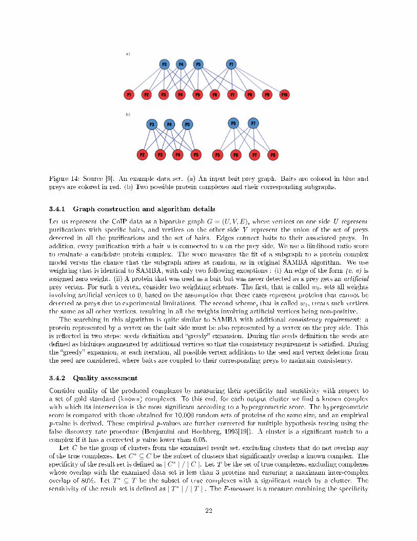
Figure 14: Source [9]. An example data set. (a) An input bait-prey graph. Baits are colored in blue andpreys are colored in red. (b) Two possible protein complexes and their corresponding subgraphs.

3.4.1 Graph construction and algorithm details

Let us represent the CoIP data as a bipartite graph G = (U, V,E), where vertices on one side U representpuri�cations with speci�c baits, and vertices on the other side V represent the union of the set of preysdetected in all the puri�cations and the set of baits. Edges connect baits to their associated preys. Inaddition, every puri�cation with a bait u is connected to u on the prey side. We use a likelihood ratio scoreto evaluate a candidate protein complex. The score measures the �t of a subgraph to a protein complexmodel versus the chance that the subgraph arises at random, as in original SAMBA algorithm. We useweighting that is identical to SAMBA, with only two following exceptions : (i) An edge of the form (v, v) isassigned zero weight. (ii) A protein that was used as a bait but was never detected as a prey gets an arti�cialprey vertex. For such a vertex, consider two weighting schemes. The �rst, that is called w0, sets all weightsinvolving arti�cial vertices to 0, based on the assumption that these cases represent proteins that cannot bedetected as preys due to experimental limitations. The second scheme, that is called w1, treats such verticesthe same as all other vertices, resulting in all the weights involving arti�cial vertices being non-positive.

The searching in this algorithm is quite similar to SAMBA with additional consistency requirement : aprotein represented by a vertex on the bait side must be also represented by a vertex on the prey side. Thisis re�ected in two steps: seeds de�nition and �greedy� expansion. During the seeds de�nition the seeds arede�ned as bicluiqes augmented by additional vertices so that the consistency requirement is satis�ed. Duringthe �greedy� expansion, at each iteration, all possible vertex additions to the seed and vertex deletions fromthe seed are considered, where baits are coupled to their corresponding preys to maintain consistency.

3.4.2 Quality assessment

Consider quality of the produced complexes by measuring their speci�city and sensitivity with respect toa set of gold standard (known) complexes. To this end, for each output cluster we �nd a known complexwith which its intersection is the most signi�cant according to a hypergeometric score. The hypergeometricscore is compared with those obtained for 10,000 random sets of proteins of the same size, and an empiricalp-value is derived. These empirical p-values are further corrected for multiple hypothesis testing using thefalse discovery rate procedure (Benjamini and Hochberg, 1995[19]). A cluster is a signi�cant match to acomplex if it has a corrected p-value lower than 0.05.

Let C be the group of clusters from the examined result set, excluding clusters that do not overlap anyof the true complexes. Let C∗ ⊆ C be the subset of clusters that signi�cantly overlap a known complex. Thespeci�city of the result set is de�ned as | C∗ | / | C |. Let T be the set of true complexes, excluding complexeswhose overlap with the examined data set is less than 3 proteins and ensuring a maximum inter-complexoverlap of 80%. Let T ∗ ⊆ T be the subset of true complexes with a signi�cant match by a cluster. Thesensitivity of the result set is de�ned as | T ∗ | / | T ||. The F-measure is a measure combining the speci�city

22

Figure 15: CoIP datasets

and sensitivity measures. It is de�ned as the harmonic average of these two measures:

2 ∗ specificity ∗ sensitivityspecificity + sensitivity

(20)

In addition, let's de�ne also accuracy measure. This measure also evaluates the quality of complexpredictions against a gold standard set. The accuracy measure is the geometric mean of two other measures:positive predictive value (PPV) and sensitivity. PPV measures how well a given cluster predicts its bestmatching complex. Let Ti,j be the size of the intersection between the ith annotated complex and the jth

complex prediction. Denote

PPVi,j =Ti,j∑ni=1 Ti,j

=Ti,j

Tj(21)

where n is the number of annotated complexes, and Tj is the sum of the sizes of all of cluster j intersectionsizes. The PPV of a single cluster j is de�ned as

PPVj =n

maxi=1

PPVi,j (22)

The general PPV of the complex prediction set is de�ned by

PPV =

∑mj=1 TjPPVj∑m

j=1 Tj(23)

where m is the number of complex predictions.The accuracy measure can be in�uenced by small and insigni�cant intersections of a predicted complex

and an annotated one. For example, if a predicted complex intersects only one annotated complex, and thesize of the intersection is 1, the PPV of that predicted complex will be 1.0. Thus, we could de�ne a thresholdto limit the e�ect of such small intersections, and evaluate the di�erent solutions under varying thresholds.

3.4.3 Datasets used

• Gold standard complexes

� 229 complexes from the MIPS database

� 193 Gene Ontology complexes from the Saccharomyces Genome Database

• CoIP datasets (Figure 15)

3.4.4 Results comparison

Now, let's show results of comparison of protein complex identi�cation approaches with CODEC algorithm.For each method we show the sensitivity of the output solution as a function of one minus its speci�city. ForCODEC we show two receiver operating characteristic (ROC) curves, corresponding to di�erent weightingstrategies (w0 and w1). The evaluation is based on a comparison to known protein complexes. The CODECplots are smoothed using a cubic spline.

23

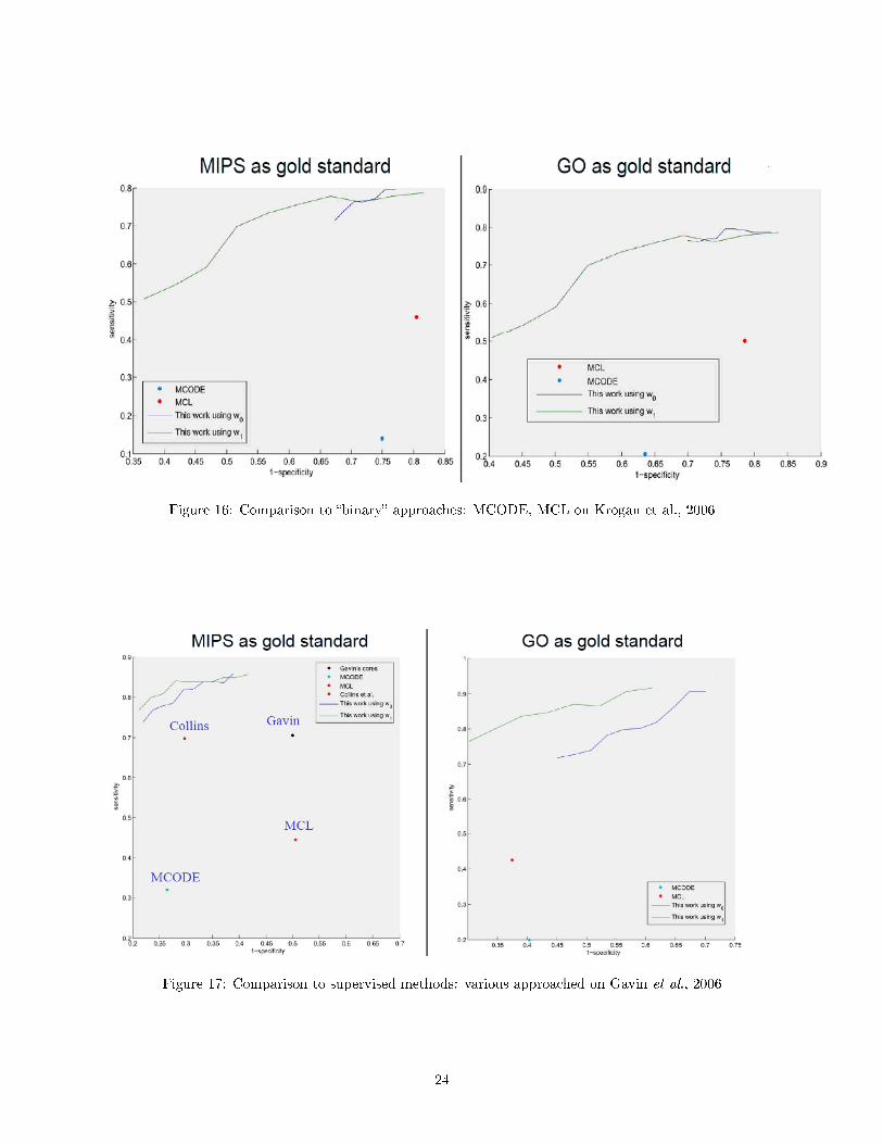
Figure 16: Comparison to �binary� approaches: MCODE, MCL on Krogan et al., 2006

Figure 17: Comparison to supervised methods: various approached on Gavin et al., 2006

24

References

[1] J. Besag. Spatial interaction and statistical analysis of lattice systems. J. Royal Statistical Society,36(2):192�236, 1974.

[2] H.N. et al Chua.

[3] Bader Gary D. and Hogue Christopher WV. An automated method for �nding molecular complexes inlarge protein interaction networks. Bioinformatics, 4(2), 2003.

[4] Giaever G. et. al. Functional pro�ling of the saccharomyces cerevisiae genome. Nature, 418:387�391,2002.

[5] Ho Y. et. al. Systematic identi�cation of protein complexes in saccharomyces cerevisiae by mass spec-trometry. Nature, 415:180�183, 2002.

[6] Lee T.I. et. al. Transcriptional regulatory networks in saccharomyces cerevisiae. Science, 298:799�804,2002.

[7] Mewes H.W. et. al. Mips: analysis and annotation of proteins from whole genomes. Nucleic Acids Res.,32:D41�D44, 2004.

[8] Uetz P. et. al. A comprehensive analysis of protein-protein interactions in saccharomyces cerevisiae.Nature, 403:623�627, 2000.

[9] Geva G. and Sharan R. Identi�cation of protein complexes from co-immunoprecipitation data. Bioin-formatics, 2009.

[10] H. Hishigaki, K. Nakai, T. Ono, A. Tanigami, and T. Takagi. Assessment of prediction accuracy ofprotein function from protein-protein interaction data. Yeast, 18(6):523�31, 2001.

[11] Newman M. E. J. Modularity and community structure in networks. PNAS, 103(23):8577�8582, 2006.

[12] Bafna V. Kalaev M. and Sharan R. Fast and accurate alignment of multiple protein networks. RECOMB,2008.

[13] E. Nabieva, K. Jim, A. Agarwal, B. Chazelle, and M. Singh. Whole-proteome prediction of proteinfunction via graph-theoretic analysis of interaction maps. Bioinformatics, 21:302�310, 2005.

[14] Girvan M. Newman M. E. J. Fast algorithm for detecting community structure in networks. Phys. Rev.E, 69(6):026113, 2004.

[15] B. Schwikowski, P. Uetz, and S. Fields. A network of protein-protein interactions in yeast. Nat Biotech-nol, 18(12):1257�61, 2000.

[16] Kupiec M. Tanay A., Sharan R. and Shamir R. Revealing modularity and organization in the yeastmolecular network by integrated analysis of highly heterogeneous genome-wide data. Proceedings of theNational Academy of Sciences, 101(9):2981�2986, March 2004.

[17] Sharan R. Tanay A. and Shamir R. Discovering statistically signi�cant biclusters in gene expressiondata. Bioinformatics, 18:136�144, 2002.

[18] Sharan R. Tanay A. and Shamir R. Biclustering algorithms: A survey. Handbook of ComputationalMolecular Biology, 2005.

[19] Benjamini Y. and Hochberg Y. Controlling the false discovery rate: A practical and powerful approachto multiple testing. J. Roy. Stat. Soc. B Met., 57:289�300, 1995.

[20] Cheng Y. and Church G.M. Biclustering of expression data. In Proc, ISMB'00 AAAI Press:93�103,2000.

25