Analysis of an Exact Fractional Step Method - University of

Art Checklist

Journal Code: JCPHArticle No: 7087

Disk Recd Disk Disk UsableArt # Y/N Format Y/N RemarksFig.1 NFig.2 NFig.3 NFig.4 Y WMF YFig.5 Y WMF YFig.6a Y WMF Y Fig.6b Y WMF YFig.7 Y WMF Y

Note:1. .eps and .tif are preferred file formats.2. Preferred resolution for line art is 600 dpi and that for Halftones is 300 dpi.3. Art in the following formats is not supported: .jpeg, .gif, .ppt, .opj, .cdr, .bmp, .xls, .wmf and pdf.4. Line weight should not be less than .27 pt.

P1: HAB Qu: 1, 3, 6, 11, 13, 18, 21

May 21, 2002 19:12 APJ/Journal of Computational Physics jcph7087

Journal of Computational Physics179,1–17 (2002)doi:10.1006/jcph.2002.7087

Analysis of an Exact Fractional Step Method

Wang Chang,∗ Francis Giraldo,† and Blair Perot∗∗Department of Mechanical and Industrial Engineering, University of Massachusetts, Amherst, Massachusetts

01003-2210; and†Naval Research Laboratory, Monterey, California Au: Pls give zip codeE-mail: [email protected]

Received June 1, 2001; revised January 8, 2002

An exact fractional step or projection method for solving the incompressibleNavier–Stokes equations is analyzed. The method is applied to both structured andunstructured staggered mesh schemes. There are no splitting errors associated withthe method; it satisfies the incompressibility condition to machine precision and re-duces the number of unknowns. The exact projection technique is demonstrated ona two-dimensional cavity flow and a multiply connected moving domain with a freesurface. Its performance is compared directly to classic fractional step methods andshown to be roughly twice as efficient. Boundary conditions and the relationship of themethod to streamfunction-vorticity methods are discussed.c© 2002 Elsevier Science (USA)

Key Words:fractional step method; projection method; incompressible; numerical;unstructured; Navier–Stokes.

1. INTRODUCTION

The incompressible Navier–Stokes equations in primitive variables are well-known andgiven by the equations

∂u∂t+ u · ∇u = −∇ p+ n∇2u,

(1)∇ · u = 0,

whereu is the velocity vector,p is the pressure (divided by density), andn is the kinematicviscosity. The numerical solution of these equations represents a difficult computationalchallenge. The problem stems largely from the pressure term in the momentum equations,which couples the momentum equations and which must be implicitly updated for incom-pressibility to be satisfied. The resulting discrete system of equations for the pressure andtwo or three velocity components is elliptic, large, indeterminate, and generally difficult tosolve efficiently. Projection methods or fractional step methods were conceived to remove

1

0021-9991/02 $35.00c© 2002 Elsevier Science (USA)

All rights reserved.

P1: HAB


2 CHANG, GIRALDO, AND PEROT

most of these computational difficulties, and to allow the system to be solved as a seriesof individual uncoupled advection–diffusion equations for each of the velocity componentsand as a Poisson equation for the pressure or for a pressurelike variable. Fractional stepmethods allow existing computational machinery for advection–diffusion equations andthe Poisson equation to be rapidly applied to solving the Navier–Stokes equations. Theprice is a certain loss of temporal accuracy in the solution, which is the subject of manyarticles [1–3] and some debate about how boundary conditions should be specified [4–6],which may now be largely resolved [7, 8], and some difficulties if convection is treatedimplicitly [9]. These are minor issues in most respects compared to the computationalsavings and code simplicity that the method produces, and so it is not surprising that frac-tional step methods are a popular technique for solving the incompressible Navier–Stokesequations.

This work focuses on the application of a new type of fractional step (or projection)method that is exact in the sense that it does not display any “splitting error,” and whichmay result in reduced computation costs. It is believed that the method is quite general andapplicable to systems based on almost any spatial discretization scheme. When appropriate,general statements about the method are made. However, some of the specific details of themethod are intricate, and for the sake of concreteness, the formal analysis and computationalresults that are presented herein focus on exact fractional step methods in the context ofstaggered mesh spatial discretizations. Staggered mesh discretizations are very frequentlyused in conjunction with fractional step methods because they do not require pressurecoupling terms to stabilize the pressure solution.

Section 2 presents a review of classic fractional step methods, since this is the standardAu: okay?

against which this new methodology is compared. Section 3 discusses some importantdetails of the staggered mesh spatial discretization, which are necessary for the reader tofully understand the motivation behind the exact projection method discussed in Section 4.Section 5 shows an example of the method applied to a complex flow problem, and Section 6discusses the accuracy and efficiency of the method. A discussion of the exact projectionmethod and its relation to other numerical techniques is presented in Section 7.

2. CLASSIC FRACTIONAL STEP METHODS

Fractional step methods (or projection methods) were originally presented and analyzedas semidiscrete approximations to the Navier–Stokes equations [10, 11]. The semidiscreteapproach discretizes the equations in time but leaves spatial derivatives as continuous oper-ators. The appeal of such a formulation is that the analysis is independent of any particularspatial discretization. It can be applied equally well to finite elements, staggered meshes, orspectral methods. The primary disadvantage of the semidiscrete approach (and one whichnecessitates that the current analysis be applied to the fully discrete system) is that it alsoleads to a great deal of confusion. Continuous differential operators require boundary con-ditions whereas discrete operators (basically matrices) do not. If the semidiscrete systemis analyzed, then boundary conditions on intermediate variables must be posed and areinvariably ambiguous. Intermediate variables in the fully discrete analysis (vectors) areunambiguously defined. Furthermore, continuous differential operators have commutativeand associative properties which are rarely shared by their discrete counterparts. This leadsto deceptive conclusions about the order of accuracy of the method when it is applied inpractice to fully discrete systems [12].

P1: HAB


AN EXACT FRACTIONAL STEP METHOD 3

When fully discretized the incompressible Navier–Stokes equations shown in Eq. (1) canbe represented in the generic matrix form,[

A GD 0

][un+1

q

]=[

r n

0

]+[

bc1

bc2

], (2)

whereA is the implicit operator for the advection–diffusion part of the momentum equations,G is the gradient operator,D is the divergence operator,r n is the explicit right-hand side ofthe momentum equations,bc1 is the boundary condition vector for the momentum equations,andbc2 is the boundary condition vector for the incompressibility constraint. Note thatAis a square matrix butG andD are not. The goal of any numerical method is to solve forthe vector of velocity unknownsun+1 and pressure unknownsq. No time level is placed onthe pressure unknown to emphasize that this unknown is simply a Lagrange multiplier thatis present so that the discrete incompressibility constraint is satisfied. Ifr n does not containan explicit pressure gradient term thenq ≈ pn+1/2. If r n has a term of the form−Gpn, thenq ≈ pn+1/2− pn. This latter form can reduce the subsequent fractional step splitting errorso that it is second order in time [8, 13].

The advantage of the semidiscrete analysis (independent of any particular spatial dis-cretization) is retained in the fully discrete analysis represented by Eq. (2), since the discretematrix operators described above can represent any discretization scheme. Eventually, wewill need to be much more specific about the exact form of the gradient and divergenceoperators, but for the purpose of understanding the classic fractional step method, they mayremain quite generic.

The detailed structure of the matrixA depends a great deal on the specifics of the timeadvancement scheme and the mesh. The most common formulation is to keep convectionexplicit and require diffusion to be implicit to avoid the stringent time-step restrictionsassociated with that term. In that case,A can be written asI/1t − nL , whereI is the identitymatrix,L is the Laplacian operator, andn is the kinematic viscosity. If the mesh is Cartesianand staggered, or unstructured and colocated, then velocity components are uncoupled ineach direction andA is block diagonal with one block for each coordinate direction. If afinite element discretization is assumed, then the identity matrix becomes a mass matrix,A = M/1t − nL , whereM is the mass matrix. If convection is also made implicit thenA = M/1t − nL + N, whereN is a linearized convection operator. The convection operatorN can be specified so thatA is still block diagonal, but this reduces the temporal accuracyof the method to first order.

As shown in Refs. [7, 14], fractional step methods are related to the block LU factorizationor Eq. (2), [

A 0D −DA−1G

][I A −1G

I

][un+1

q

]=[r n

0

]+[

bc1

bc2

]. (3)

While Eq. (3) is exact, and is sometimes referred to as the Uzawa method, it is not the basisfor a practical computational method because computing the inverse of the matrixA is veryexpensive. Practical methods for solving Eq. (2) usually approximateA−1 with the matricesB1 andB2, and then (3) can be rewritten as

Aw = r n + bc1,

DB1Gq = Dw, (4)

un+1 = w − B2Gq.

P1: HAB



Different approximations to the two matrix inverses result in different classes of frac-tional step methods. The classic fractional step method approximation isB1 = B2 = 1t I .If q ≈ pn+1/2 this results in a first-order error term in the momentum equation, and ifq ≈ pn+1/2− pn this results in a second-order error term in the momentum equation. Ifthe approximate inverses are equal (B1 = B2), then all the error in the approximation ap-pears in the momentum equation and discrete continuity is satisfied exactly. However, ifthe approximate inverses are chosen to be different (such asB1 = 1t I andB2 = A−1),then the splitting error term can be moved entirely from the momentum equation so that itAu: okay?

appears only in the incompressibility constraint. It is not entirely clear which type of error(momentum or divergence error) is the least detrimental. In all probability, the answer tothat question is problem dependent. However, the most frequent assessment is that massshould be conserved and the splitting error is best placed in the momentum equation (withB1 = B2). Antidotal evidence which confirms the detrimental nature of mass conservationerror (versus momentum errors) is found in Section 6 of this paper, where we look at theerror that results from solving the elliptic Possion equation with an iterative method tosome small but finite error tolerance. Higher order splitting methods can be constructedby constructing higher order approximations toA−1 [7]. It is also important to note thatthe intermediate variable,w, does not require boundary conditions; it is simply a way ofrewriting Eq. (3).

Fractional step methods are also referred to as projection methods because the system ofequations given by (4) can be interpreted as projection in velocity space. The “trial velocity,”w, is an approximate solution to the momentum equations, but because the trial velocityis obtained with an explicit pressure it cannot satisfy the incompressibility constraint atthe next time level. The Poission equation (second equation) determines the minimumperturbation that will make the trial velocity incompressible, and the final equation perturbsthe trial velocity to obtain the final velocity. Only ifB1 = B2 = A−1 is the classical fractionalstep method free from splitting errors. Because the exact projection method presented inSection 4 is constructed in a manner entirely different from classic fractional step methodsit remarkably avoids the need for constructingA−1 or any approximations toA−1 whileeliminating any splitting error.

3. STAGGERED MESH DISCRETIZATION

Fractional step methods are a technique for dealing with the pressure and the incom-pressibility constraint and can be applied to any discretization scheme. However, for claritywe need to discuss a particular discretization scheme. Staggered mesh schemes of the typeintroduced by Harlow & Welch [15] are frequently used in conjunction with fractional stepmethods. The exact projection method and accompanying examples will therefore be pre-sented in the context of the staggered mesh discretization. We consider both unstructuredtwo-dimensional and three-dimensional staggered meshes in order to keep the discussionas general as possible. The unstructured analysis is, of course, applicable to structuredCartesian meshes as a subclass.

Staggered mesh schemes display a number of mathematical and physical properties whichmake them attractive for solving the incompressible Navier–Stokes equations. Foremost inthe context of incompressibility is the fact that these discretizations do not display spuriouspressure oscillations and therefore do not require pressure coupling terms. In addition,they have low memory requirements, are computationally efficient, and display a number

P1: HAB



FIG. 1. Location of face normal velocity components and pressure unknowns in a two-dimensional unstruc-tured mesh.

of interesting conservation properties, including conservation of mass, momentum, kineticenergy, and vorticity [16]. Unstructured staggered mesh schemes are still under development[17, 18] but can also possess very attractive numerical properties [19].

The common aspect of both Cartesian and unstructured staggered mesh methods is that theprimary unknowns of the method are the normal velocity components, located at mesh faces.Pressure and other scalar variables are located at the center of mesh cells in a manner akin tostandard finite volume methods. The velocity vector in the mesh cell must be reconstructedfrom the face normal components, and it is the different reconstruction methods that lead todifferent types of staggered mesh methods with different numerical properties. The locationof variables in a two-dimensional staggered mesh is shown in Fig. 1.

On a staggered mesh, the incompressibility constraint is imposed on average in each meshcell. Gauss’s divergence theorem can be used to convert the incompressibility constraintinto integration over the cell faces:

0=∫

cell

∇ · u dV =cell

faces∑ ∫facei

u · n dS. (5)

If the normal velocity is assumed to vary linearly on the face (a second-order approximation),then the integration can be performed analytically and the incompressibility constraintbecomes a simple summation over the primary velocity unknowns,

0=cell

faces∑u Af, (6)

whereAf is the cell face area and the circumflex (hat) on the velocity indicates that this isthe normal velocity component pointingout of the cell in question. If Eq. (6) is applied toevery cell in the mesh at the final time level, then a matrix system is obtained,DUn+1

f = 0,whereUf = u Af is the mass flux through the face. The matrixD is sparse and nonsquare.For the simple mesh shown in Fig. 1, the matrixD has the form

D =[

1 0 0 1 1−1 1 1 0 0

]. (7)

In generalD has nonzero entries that are either+1 or−1 (−1 if the face normal vector pointsinto the cell). It hasNf columns, whereNf is the number of faces in the mesh, andNc rows,

P1: HAB



whereNc is the number of cells. Every column ofD that corresponds to an internal meshfaces will have a single+1 and a single−1 entry. Every column ofD that corresponds to amesh face on the boundary of the computational domain will only have one nonzero entry,and if the normal vector is assumed to point out of the computational domain that entrywill be +1. The matrixD will behave like a discrete divergence operator, but it should benoted that it has been stripped of its geometric variables (the face area and cell volume). Thenegative transpose of the divergence operator is a gradient operator,G = −DT . On interiorfaces this operator takes the difference of the two neighboring cell values. On boundaryfaces it takes the negative of the value of the interior cell. The gradient operator for Fig. 1 is

G =

−1 10 −10 −1−1 0−1 0

. (8)

A discrete system, in the form of Eq. (2), is constructed by discretizing the line integralof the momentum equation at each cell face [19, 20] and constructing a discrete equationfor the time evolution of

∫u · n dl. This gives a single equation at each mesh face; one

equation for each velocity unknown. For Cartesian meshes and unstructured meshes usingcell circumcenters, the line connecting the two neighboring cell centers is normal to theface, and the time derivative produces a diagonal matrix contribution toA. Each element ofthe diagonal matrix is1

1tL fAf

, whereL f is the distance between neighboring cell centers. Forunstructured staggered meshes using a cell position other than the cell circumcenter, thediscretization of the time derivative results in a mass matrix. The mass matrix is similar, butnot identical, to a finite element mass matrix. In either case, the matrixA is square and hasa sizeNf by Nf . It should also be noted that the line integral of the pressure gradient in themomentum equation is exactly equal to the difference of the pressure at the two cell centers,so the pressure discretization is, in some sense, exact for staggered mesh formulations.

With this discretization scheme, the matrix equations that must be solved are written as[A G−D 0

][Un+1

f

q

]=[

r n

0

]−[

qb

0

]. (9)

It should be noted that for simplicity, the matrix system as it is now posed includes all themesh faces, including those on the boundary that may actually be known. This eliminatesany explicit boundary condition treatment of the incompressibility constraint. We have alsochosen (purely for aesthetic reasons) to multiply the divergence-free constraint by−1. Thismeans that ifA is symmetric (explicit convection), then the entire system is also symmetric.The entire system is also square and has a sizeNc+ Nf by Nc+ Nf . On a boundary wherethe normal velocity is not known, such as a moving free surface or an outflow boundary, itis often convenient to specify the boundary pressure. This boundary pressure is located atthe cell faces, or more logically in infinitesimally thin virtual boundary cells that surround thedomain. These boundary pressures are explicitly represented in Eq. 9 by the vectorqb. Theminus sign on this term assumes that boundary normals point outward. This notation alsoimplies that the right-hand-side vectorr n now only has contributions from the velocity field,not the pressure field. A more detailed discussion of specific staggered mesh discretizationscan be found in Refs. [17–21].

P1: HAB



4. EXACT PROJECTION METHOD

Classic fractional step methods can never be exact because each conservation equa-tion (momentum, then continuity) is satisfied sequentially. Satisfaction of one equationproduces error in the solution of the other equation. One way to enforce both mass andmomentum conservation and evolve the system at the same time (and without any associ-ated error) is to assume the solution lies in a function space that is already incompressible.In the finite element context this is equivalent to assuming basis functions which alreadysatisfy incompressibility. However, standard conforming basis functions which satisfy theincompressibility constraint have never been particularly popular because they require basisfunctions which are at least fourth-order polynomials [22]. Nonconforming (discontinuous)finite element spaces have been proposed [23] that have some similarities to the proposedmethod. In this section, we show that low-order finite volume basis functions can be easilyconstructed which satisfy the constraint ofdiscreteincompressibility.

The method relies on the fact that matrixD is wider than it is tall and therefore defines anull space. The null space is the maximal set of linearly independent vectors that equal zerowhen they are multiplied by the matrixD. The null space ofD is therefore another nonsquarematrix with a heightNf . There are many possible null spaces, but we define an easilyconstructed null spaceC. In two dimensions,C hasNn columns, whereNn is the numberof nodes (vertices) in the mesh. In three dimensions, it hasNe columns, whereNe is thenumber of edges. The matrixC acts like a discrete curl operator. In two dimensions it has twoentries in every row, one+1 and one−1. The+1 corresponds to the node 90 degrees fromthe normal vector at the face in question, and the−1 corresponds to the node that is−90 degrees from the normal vector. In three dimensions there is one entry for each edgewhich forms the face in question, and the entry is+1 if that edge points counterclockwisewith respect to the face normal, and it is−1 if the edge points clockwise with respect tothe face normal. In the interior of the domain, both the edge directions and face normals arechosen arbitrarily from the two possible choices for each. There is no logical way to choosethese directions in three dimensions. The curl matrix,C, for the mesh shown in Fig. 1 is

C =

1 0 −1 01 −1 0 00 1 −1 00 0 1 −1−1 0 0 1

. (10)

Using the curl matrix, we can guarantee by construction thatDC = 0. The result is alwayszero, because each row is a closed summation over differences, and the differences allcancel out with one positive and one negative. The presence of the matrixC is not exclusiveto staggered mesh discretizations. All discrete divergence operators have a null space. Thestaggered mesh discretization just makes the construction of the null space very simple andmakes it clear that the null space,C, is a discrete curl operator. An example of the curloperator for irregular quadrilateral meshes is discussed in Hyman and Shashkov [24]. Thebasic idea of using a null space dates back to Hallet al. [25].

The discrete curl operator allows us to define a discrete streamfunction vector. We willassume thatUf = Cs, wheres is the discrete streamfunction. In two dimensions the stream-function points out of the two-dimensional plane and is located at the mesh nodes. In three

P1: HAB



dimensions the discrete variable,s, actually represents the streamfunction vector integratedalong the edge,s= ∫edge9 · dl. Irrespective of its physical interpretation, this mathematicalconstruction guarantees discrete incompressibility (DUf = DCs= 0s= 0).

It is important that the curl operator be complete. That is, its columns should spanthe entire null space which has a sizeNf − Nc. In two dimensions, one of Euler’s manyAu: as meant?

formulas tells us thatNf − Nc = Nn− 1+ Nh, whereNh is the number of holes in a possiblymulticonnected domain. In three dimensions we haveNf − Nc = Ne− Nn− 1+ Nh. SinceC hasNn columns in two dimensions andNe columns in three dimensions there are alwaysmore columns than necessary to span the null space if the domain does not contain holes.The−1 in the 2D formula is an indication that the streamfunction is only defined up toan arbitrary constant; the−Nn− 1 in 3D is a reflection that the streamfunction in threeAu: as meant?

dimensions is only defined up to an arbitrary gradient. These properties of the discretestreamfunction are true for the continuous streamfunction as well. When holes are presentin the domain, the presence ofNh indicates that certain other constraints are automaticallysatisfied by this particular construction. In particular, the net mass flux into or out of a holein the domain must always be zero using this construction for the velocity.

Automatically satisfying the incompressibility constraint is only half the goal of the exactprojection procedure. The other goal is to eliminate the pressure. This is done by notingthat the gradient operator is the negative transpose of the divergence operator. The gradientoperator is therefore the null space of another matrix operator,R, (0T = (DC)T = CTDT =−RG). The rotation operatorR = CT is another type of curl operator. It hasNf columnsand Ne (or Nn in 2D) rows. Each column has one nonzero entry for every edge (in 3D)or node (in 2D) which the face touches. The sign is given by the same convention as thecurl operator. For interior edges, the rotation operator defines a complete counterclockwisecircuit around and edge (in 3D) or node (in 2D). At boundary edges or nodes, these circuitsare not complete, but begin and end with the boundary faces touching that edge or node.

Applying these operators to the discrete system given by Eq. (9) gives

[RA RG−D 0

][Csn+1

q

]=[

Rr n

0

]−[

Rqb

0

]. (11)

The off-diagonal terms in the matrix are now zero, so the exact fractional step method is

RACsn+1 = R(r n − qb),(12)

un+1f = 1

AfCsn+1.

This is an exact projection which inverts both the matrixA and the Poisson equation (RC)at the same time. There are no approximations to any of the matrices and so there is nosplitting error. Note that all the matrix operators involved are sparse and only require nearest-neighbor communication. IfA is symmetric (explicit convection), then the total system isalso symmetric. IfA is positive semidefinite (implicit upwind convection), then the totalsystem is also positive semidefinite. So any matrix inversion technique which is appropriatefor A is also appropriate for the total system,RAC. In the example problems described inSection 5, this system is solved using a Jacobi preconditioned conjugate gradient solver,but the exact matrix solution choice is not critical to the exact projection method.

P1: HAB



4.1. Comparison with Classical Fractional Step Methods

Classic fractional step methods require inverting the matrixA and then solving a separatePoisson equation for the pressure variable. If the viscosity is small and the convection termis explicit, then the matrixA is highly diagonally dominant (due to the time derivative term)and an iterative solution can be obtained in very few iterations. Large viscosity or implicitconvection will require more iterations. Cartesian meshes speed the solution by allowingAto be decomposed for each velocity direction, and allowing the diffusion to be approximatedby a series of tridiagonal matrices in each coordinate direction. The bulk of the computationaleffort of classic fractional step methods therefore lies in the solution of the Poisson equation.The solution of the Poisson equation can only be simplified in very special geometries(periodic uniform Cartesian meshes). Usually, it requires solution via iterative methods,either Krylov subspace methods (typically conjugate gradients) or multigrid relaxationschemes. The Krylov methods will require on the order of

√Nc iterations in 2D and onAu: as meant?

the order ofNc work per iteration, since there areNc pressurelike unknowns in the Poissonequation.

The work involved in solving the exact projection method will be very similar to solvinga simple Poisson equation ifA is very diagonally dominant, which it frequently is. However,the number of iterations and the work per iteration now scales with the number of nodes,Nn

(in 2D), or the number of edges,Ne (in 3D). Table I shows a comparison of the number ofstreamfunction unknowns versus the number of pressure unknowns for various dimensionsand meshes. This gives a good indication of the relative cost per iteration, and some idea asto the number of iterations required to achieve convergence. Note that the exact projectionmethod is equal or lower in cost per iteration for unstructured meshes or 2D Cartesianmeshes but requires more work per iteration for Cartesian meshes in three dimensions.

The number of iterations is also an important issue. The exact method requires slightlymore work per iteration because the matrixA is imbedded in the inversion. However, thePoisson equation in the classic fractional step method must be converged to very tighttolerances requiring numerous iterations. In the classic fractional step method small errorsin the Poisson solution lead to relative large numerical divergence or local mass creation, andto significant errors in the resulting velocity field. It is hypothesized (with some evidencegiven in Section 6) that far fewer iterations are required for the exact projection method. Theexact projection maintains exact incompressibility (local mass conservation), even when thesolution is not fully converged. Error appears as error in the vorticity, not the dilatation, and isexpected to be less detrimental to the final solution in most cases. Therefore, the convergencetolerances acceptable in the exact projection method are larger (and the number of iterationsfewer) than what is required to obtain solutions via the classical fractional step method.

While the exact method introduces a new variable, it also eliminates the need to store thepressure in the domain (however boundary pressures may still be retained). So the overall

TABLE I

Number of Edges (3D) or Nodes (2D) Divided

by the Number of Cells

Cartesian Unstructured

2D 1 0.53D 3 ≈1

P1: HAB



storage requirements are not expected to be fundamentally different. If pressure is required,it can still be obtained from the exact projection method. However, it is a postprocessingstep, which can occur as infrequently as desired and which does not affect the velocity fieldevolution.

One final advantage of classic fractional step methods may be their conceptual simplic-ity. However, while the novelty of the exact projection method may make it appear lessstraightforward, it is not fundamentally more complex to understand or implement thanclassic fractional step methods.

4.2. Boundary Conditions

The use of the streamfunction,s, as the primary unknown rather than the normal ve-locity components complicates some boundary conditions and simplifies others. There aretwo types of boundary conditions on the velocity: the inviscid boundary condition on thenormal velocity, and the viscous condition applied to the tangential velocity components.The viscous boundary condition is the boundary condition that disappears when the Euler(inviscid Navier–Stokes) equations are solved and it is not affected by the change in theprimary variable. It is the inviscid boundary condition that is of concern in this section.

Boundary conditions in which the streamfunction is known are trivial to implement inthe exact projection method. A solid wall (without transpiration) or a stationary free sur-face is streamline and can be represented by a constant streamfunction value. A knowninflow velocity (or transpiration velocity) can often be analytically converted into a knownstreamfunction profile (by numerical or analytical integration). Note that where the stream-function or normal velocity is fixed on the boundaries, the boundary pressure does notaffect the solution and is not required. However, outflow boundary conditions and mov-ing free surfaces are easily implemented by fixing the boundary pressure and allowing theboundary streamfunction (and resulting boundary normal velocity) to be left as unknowns.Inflow boundaries (potential inflow) can also be implemented by specifying the dynamicpressure rather than the streamfunction; this allows fluid to be sucked into the domain bya momentum source in the interior. Walls in the interior of the domain (causing multiplyconnected domains) are the most difficult to specify. These walls have a constant stream-function value, but that value is unknown and can change with time. An example is the high-Reynolds-number flow perpendicular to a long cylinder. The streamfunction on the cylinderchanges as the resulting Von Karman vortex street oscillates back and forth. The systemof equations for this boundary condition is created by allowing one streamfunction on theinterior wall to remain unknown and specifying that all other streamfunction values on thewall are equal to that unknown value. Careful examination of such a boundary conditionsshows that this approach is equivalent to specifying the line integral around the object.Consequently, boundary pressure on interior objects is not required. In summary, pressureboundary conditions can be specified if so desired (often they are very convenient), but theyare not required. The second example problem in Section 5 demonstrates most of theseboundary conditions, including the difficult case of an interior wall and a moving boundary.

5. EXAMPLE PROBLEMS

A test of the exact projection method was performed on two-dimensional cavity flow ata Reynolds number of 100. This is a test case that has been computed extensively in thepast and is well understood. An unstructured mesh containing roughly 4024 triangles and

P1: HAB



FIG. 2. Unstructured mesh and boundary conditions used to calculate driven cavity flow at a Reynolds numberof 100.

2013 nodes was used for the calculation and is shown in Fig. 2. Since no fluid leaves thecavity, the streamfunction is zero on the boundary. The primary vortex center was computedto be at (0.6166, 0.7477) when the coordinate system is located at the bottom left corner ofthe cavity. This compares well with the predictions of Ghiaet al. [26], who report a vortexcenter at (0.6172, 0.7344) using 128× 128 Cartesian mesh resolution. Cross sections ofthe steady state velocity profiles at the two midlines are shown in Fig. 3. Figure 3a showsthe horizontal velocity on the liney = 0.5, and Fig. 3b shows the vertical velocity on theline x = 0.5. The agreement with Ref. [26] is what would be expected from this level ofmesh resolution.

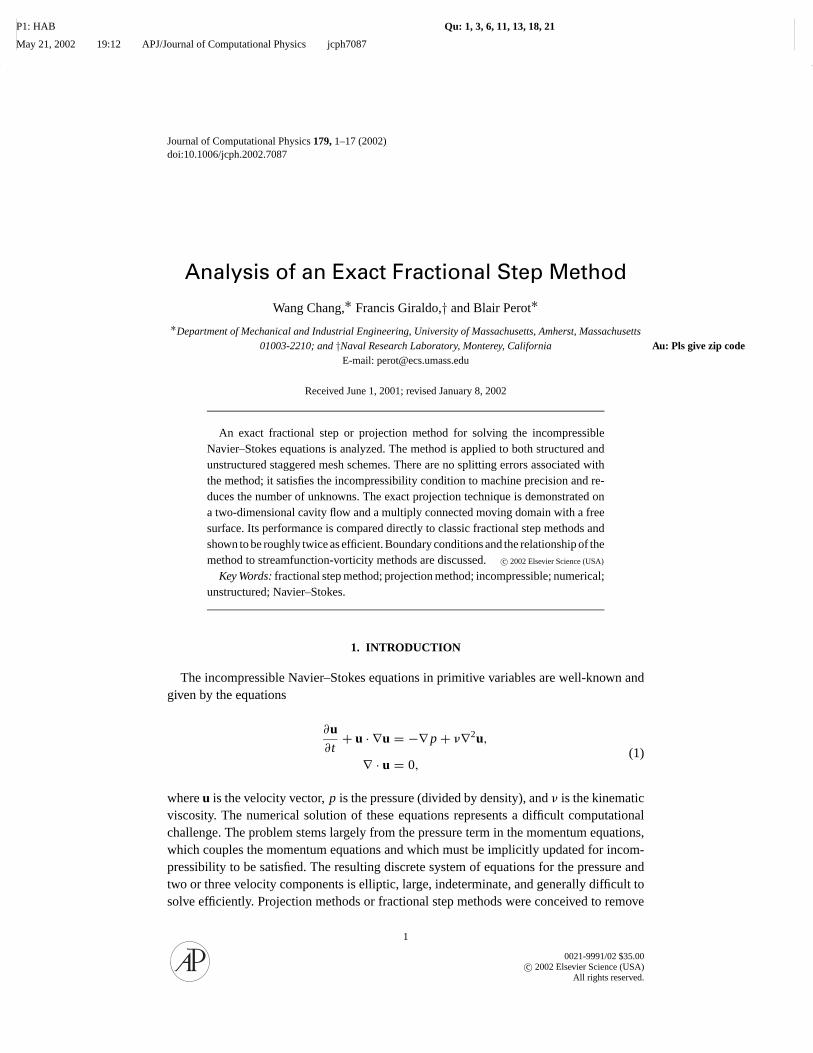
The time accuracy of the method was analyzed by looking at the cavity flow start-upprocess. The flow was initialized with zero velocity and allowed to evolve to a time of20 using different-size time steps. It takes 1000 time units for the flow to move from thetop left to the top right corner of the domain. The total kinetic energy was evaluated attime= 20 and its error is plotted in Fig. 4 versus the time step for both the exact and thefirst-order classic projection method. The exact solution was obtained by extrapolating theresults to zero time step. Since the total kinetic energy grows monotonically during this

FIG. 3. Mean flow predictions along the midlines. Lines are the exact projection method and symbols are thehigh resolution data from Ghiaet al. (a) u, Velocity parallel to moving wall; (b) v, velocity perpendicular to themoving wall.

P1: HAB



Kin

etic

En

erg

y E

rro

r

0.05 0.1 0.5 1

∆t

52E-15

1E-14

1E-13

1E-12

1E-11

1E-10

2E-10

Classic Fractional StepExact Fractional Step2nd order1st order

FIG. 4. Error in the total kinetic energy at time= 20 versus the time step.

initial start-up process it is a good global indicator of the overall accuracy of the method.The exact method shows second-order accuracy over the entire range of time steps. Theclassic method shows second-order convergence for the larger time steps (greater than 1)and then first-order convergence when the time step is very small (less than 1). Note thata time step of 1 corresponds to a maximum CFL of 0.05, which is smaller than one wouldnormally use. In the practical operating range the classic method is second-order accurate,and the splitting error only begins to dominate in this case when the CFL number is verysmall. Therefore, in this particular flow, the primary advantage of the proposed method isnot its temporal accuracy but its numerical efficiency. The classic method required very tighterror tolerances on the conjugate gradient solver in order to obtain these results. Even mode-rate tolerances resulted in erratic convergence behavior of the classical method, becausesmall errors in the Poisson solution for the pressure correction result in large errors in thevelocity. This point is discussed further in the next section.

In order to demonstrate the ability of the method to predict flows in complex domains andwith a variety of boundary conditions, the exact projection method was used to compute theflow of water around a square cylinder which is below a free surface. The mesh and initialcomputational domain are shown in Fig. 5. The flow is laminar and two dimensional butdisplays fairly complex behavior in time. An unsteady Von Karman vortex street developsbehind the cylinder with a shedding frequency that depends on the Reynolds number. Thefree-surface response to the cylinder depends on the Froude number. The simulation usesan unstructured mesh, and the mesh moves with the free surface to retain an accurate repre-sentation of the free-surface motion. The interior mesh moves and occasionally reconnectsusing a flipping algorithm to maintain a high-quality mesh in the interior. The first calcu-lation, shown in Fig. 6a, has a Reynolds number of 1000 based on the inlet velocity and

P1: HAB



FIG. 5. Mesh and initial domain for the calculation of free-surface channel flow with a submerged squarecylinder cross section.

cylinder height and a supercritical Froude number of 1.5 based on the inlet velocity andinitial channel height. The second calculation, shown in Fig. 6b, uses the same Reynoldsnumber but a subcritical Froude number of 0.75. Figures 6a and 6b show contours of thestreamwise velocity at one instant in time.

It should be noted that the streamfunction on the cylinder is constant on the cylinderbut varies in time and is therefore a more difficult boundary condition than the bottom ofthe domain, which is a slip wall (constant-in-time streamfunction). The free surface is nota streamline because it is not steady. The free surface uses a constant pressure boundarycondition (zero gage pressure in this case), and the outflow uses a constant hydrostaticpressure assumption (pressure proportional to distance below the waterline). The inflow isuniform velocity. The unsteady nature of this particular flow is a good example of whereone might be particularly concerned about time accuracy of the simulation, and where exactprojection could be of significant value. The complexity of the algorithm and resulting codeis equivalent to the classic projection method.

FIG. 6a. Prediction of the free-surface location and streamwise velocity field at Re= 1000, Fr= 1.5.

P1: HAB



FIG. 6b. Prediction of the free-surface location and streamwise velocity at Re= 1000, Fr= 0.75.

6. ANALYSIS OF CONVERGENCE ERROR

The solution of the Poisson equation, in either the classic or the exact fractional stepmethods, is almost always computed using an iterative method. Whether the iterative methodis a Krylov-based method or a multigrid scheme this invariably results in what is calledconvergence error. There is a direct trade-off between the convergence error that is toleratedand the speed of the Poisson solver (which dominates the overall solution time). It isclear from the analysis of Section 2 that convergence error in the classic fractional stepmethod appears as nonzero dilatation (or local mass creation/destruction). On the otherhand, the exact projection method maintains dilatation at machine precision at all timesand convergence error appears as erroneous vorticity. It was suggested earlier that vorticityerrors may be less detrimental to the overall flow solution than dilatation errors, therebyallowing fewer iterations for the exact projection and a faster solution than when usingthe classical projection method. In all likelihood, the exact impact of the error is problemdependent, but the test below suggests that errors in the mass cause larger errors in thevelocity field than do errors in the vorticity. So exact projection often requires far feweriterations to achieve the same accuracy in the velocity field.

To test this idea, one time step of the cavity flow problem was calculated using a fixednumber of Jacobi preconditioned CG iterations. The solution was calculated using both theproposed exact fractional step method and the classic (second order) projection method ofDukowitcz and Dvinsky [8]. All other aspects of the code remained identical. The error afterone time step was taken to be the L2 (or RMS) error of the normal velocity components overall the cell faces. The exact solution for the error calculation was assumed to be the solutionobtained after a very large number of iterations (128 iterations for the exact method and512 iterations for the classic method). Because of the splitting error in the classic method,the “exact” solutions for the two methods are not identical. The error is defined this wayon purpose. The affect of the splitting error has already been discussed. We wish to focusexclusively in this test on convergence error. This error norm gives a precise indication ofthe convergence error that results from solving an elliptic system with a finite number ofiterations. While convergence error has not been discussed in prior publications concerningfractional step methods it is of very real practical importance, since the elliptic Poisson

P1: HAB



CG iterations

L2

erro

r

0 60 120 180 240 3001E-9

1E-8

1E-7

1E-6

1E-5

0.0001

0.001

Exact ProjectionClassic Projection

FIG. 7. Error in the velocity field for a fixed number of iterations of the CG solver and one time step.

equation and the tolerances that are imposed on its solution dominate the overall solutiontimes of these methods.

A plot of the velocity error versus the number of iterations is shown in Fig. 7, for boththe exact projection method and the classic projection method. The plot indicates that theclassic projection method requires at least four times as many iterations to achieve the samelevel of accuracy in the velocity as the exact projection method. Taking into account thefact that the exact method requires more work per iteration (multiplying by the matrixA Au: bf okay? (as used in

beginning?)at each iteration) suggests that the computational advantages of the exact method will besomewhat less than this figure implies. If it is estimated that the computation ofA is roughlyequivalent to the computation of the Laplacian, then the exact projection method will beroughly twice as computationally efficient as the classic projection method for the sameconvergence error. Because the classic method solves for pressurelike variables at cells andthe exact method solves for the streamfunction at nodes (2D) or edges (3D) this statement isreally only correct for 2D Cartesian meshes and 3D unstructured meshes (see Table I). Thecomputational advantages of the exact method are actually enhanced for 2D unstructuredmeshes and possibly almost completely removed for 3D Cartesian meshes.

7. DISCUSSION

An exact projection or fractional step method for solving the incompressibleNavier–Stokes equations has been demonstrated which does not have any splitting error.The details of the method were discussed in the context of a staggered mesh discretization,but there appear to be no fundamental difficulties in applying this type of projection to otherspatial discretization schemes. The greatest hurdle of generalizing this method to otherdiscretization schemes is the construction of the divergence null space and its transpose.The null space and its transpose should preferably be sparse and explicit. It is unclear atthis time whether other discretization schemes display simple null spaces like the staggeredmesh does, but the authors would be surprised if a finite element scheme (possibly Petrov–Galerkin) could not be manipulated to do so.

The method was demonstrated on a two-dimensional cavity flow and a relatively com-plex unsteady flow in a multiconnected domain involving a moving free surface and a

P1: HAB



Von Karman vortex street. The cavity flow showed good agreement with other numericalsimulations and the free surface showed qualitatively correct behavior at both subcriticaland supercritical Froude numbers. While the demonstrations in this work are for two-dimensional flows, the exact projection scheme is currently being used in research forthree-dimensional unstructured staggered mesh simulations.

Analyses of the errors associated with using iterative solvers for the Poisson equationwere performed. The results suggest that, at least for some flows, the convergence error inthe exact method (extraneous vorticity) is more benign than that created by classic fractionalstep methods (extraneous dilatation). This allows fewer iterations of the solver and fastersolution times for a given level of accuracy.

It is obvious that the exact projection method has some relationship to streamfunctionmethods. The essential distinction is that classic streamfunction methods manipulate theNavier–Stokes equations first and then discretize those equations. The exact projectionmethod discretizes the Navier–Stokes equations first (and their boundary conditions) andonly then manipulates the equations discretely into a form very similar to a streamfunctionmethod (and using similar, but discrete, operators). This second approach eliminates twovery important disadvantages of classic streamfunction methods [27]. First, in three dimen-sions the computational effort does not grow by a factor of three from the two-dimensionalcase. This is because exact projection does not solve for the whole streamfunction vector;it just solves for the component of streamfunction along each edge. In this way, the exactprojection method applied to three-dimensional simulations is not fundamentally differentfrom two-dimensional simulations. The other advantage is that boundary conditions are ap-plied to the Navier–Stokes equations in primitive variables, so it is not necessary to specifythe streamfunction or the vorticity on the boundaries. One can specify the streamfunctionif one so desires, but it is also possible to specify the pressure or a normal velocity condi-tion. This was demonstrated by the second test problem, where the streamfunction on thecylinder, the free surface, and the outflow are not specified.

Another possible advantage of the exact projection scheme over classic fractional stepmethods (but one that is not demonstrated herein) is that implicit convection may causefewer difficulties. In classic fractional step methods, implicit convection often leads to largesplitting errors (even if the order of the error is not low). Exact projection avoids splittingerrors and therefore circumvents any problems associated with implicit convection.

While the purpose of the proposed exact method is equivalent to fractional step or pro-jection methods it is clearly no longer well described by either moniker. If there is anyprojection going on, it is a projection of the basis functions into a discretely incompressiblefunction space, rather than a projection of the solution. A more apt description of the methodwould be to refer to it as a discrete streamfunction method, or perhaps an incompressiblebasis function method.

ACKNOWLEDGMENTS

This work was supported in part by the Office of Naval Research, the Air Force Office of Scientific Research,and a grant from Aquasions Inc.

REFERENCES

1. R. Rannacher,The Navier–Stokes Equations II—Theory and Numerical Methods, Lecture Notes inMathematics (Springer-Verlag, Berlin, 1992), Vol. 1530.

P1: HAB



2. J. C. Strikwerda and Y. S. Lee, The accuracy of the fractional step method,SIAM J. Numer. Anal.37, 37(1999).

3. D. Brown, R. Cortez, and M. Minion, Accurate projection methods for the incompressible Navier–Stokesequations,J. Comput. Phys.168, 464 (2001).

4. M. Lee, B. D. Oh, and Y. B. Kim, Canonical fractional-step methods and consistent boundary conditions forthe incompressible Navier–Stokes equations,J. Comput. Phys.168, 73 (2001).

5. R. Temam, Remark on the pressure boundary condition for the projection method,Theor. Comput. Fluid Dyn.3, 181 (1991).

6. W. E. and J. Liu, Projection method. I: Convergence and numerical boundary layers,SIAM J. Numer. Anal.Au: pls spell out last name32, 1017 (1995).

7. J. B. Perot, An analysis of the fractional step method,J. Comput. Phys.108, 51 (1993).

8. J. K. Dukowitcz and A. S. Dvinsky, Approximation factorization as a high order splitting for the implicitincompressible flow equations,J. Comput. Phys.102, 336 (1992).

9. J. B. Bell, P. Collela, and H. M. Glaz, A second order projection method for the incompressible Navier–Stokesequations,J. Comput. Phys.85, 257 (1989).

10. A. J. Chorin, Numerical solution of the Navier–Stokes equations,Math. Comput.22, 745, (1968).

11. P. M. Gresho and S. T. Chan, On the theory of semi-implicit projection methods for viscous incompressibleflow and its implementation via a finite element method that also introduces a nearly consistent mass matrix.Part 2: Implementation,Int. J. Numer. Methods Fluids11, 621 (1990).

12. J. Kim and P. Moin, Application of the fractional-step method to the incompressible Navier–Stokes equations,J. Comput. Phys.59, 108 (1985).

13. J. Van Kan, A second order accurate pressure-correction scheme for viscous incompressible flow,SIAMJ. Sci. Comput.7, 870 (1986).

14. J. B. Perot, Comments on the fractional step method,J. Comput. Phys.121, 190 (1995).

15. F. H. Harlow and J. E. Welch, Numerical calculations of time dependent viscous incompressible flow of fluidwith a free surface,Phys. Fluids8(12), 2182 (1965).

16. D. K. Lilly, On the computational stability of numerical solutions of time-dependent non-linear geophysicalfluid dynamics problems,Mon. Weather Rev.93, 11 (1965).

17. R. A. Nicolaides, The covolume approach to computing incompressible flows, inAlgorithmic Trends inComputational Fluid Dynamics, edited by M. Y. Hussaini, A. Kumar, and M. D. Salas (Springer-Verlag,Berlin/New York, 1993), p. 295.

18. S. H. Chou, Analysis and convergence of a covolume method for the generalized Stokes problem,Math.Comput.66 (217), 85 (1997).

19. J. B. Perot, Conservation properties of unstructured staggered mesh schemes,J. Comput. Phys.159, 58 (2000).

20. X. Zhang, D. Schmidt, and J. B. Perot, Accuracy and conservation properties of a three-dimensional staggeredmesh scheme, submitted for publication.

21. R. A. Nicolaides, The covolume approach to computing incompressible flow, inIncompressible ComputationalFluid Dynamics, edited by M. D. Gunzburger and R. A. Nicolaides (Cambridge Univ. Press, Cambridge, UK,1993), p. 295.

22. V. Girault and P. Raviart,Finite Element Approximation of the Navier–Stokes Equations(Springer-Verlag,Berlin, 1986).

23. S. Turek, Tools for simulating non-stationary incompressible flow via discretely divergence-free finite elementmodels,Int. J. Numer. Methods Fluids18, 71 (1994).

24. J. M. Hyman and M. Shashkov, The orthogonal decomposition theorems for mimetic finite difference methods,SIAM J. Numer. Anal.36(3), 788 (1999).

25. C. A. Hall, J. C. Cavendish, and W. H. Frey, The dual variable method for solving fluid flow differenceequations on Delaunary Triangulations,Comput. Fluids20(2), 145 (1991).

26. U. Ghia, K. N. Ghia, and C. T. Shin, High Re solutions for incompressible flow using the Navier–Stokesequation and multigrid methods,J. Comput. Phys.48, 387 (1982).

27. R. Peyret and T. Taylor,Computational Methods for Fluid Flow(Springer-Verlag, Berlin, 1983).

Analysis of an Exact Fractional Step Method - University of

Documents

Transcript of Analysis of an Exact Fractional Step Method - University of