Journal of Fractional Calculus and Nonlinear Systems J Frac Calc & Nonlinear Sysjfcns.sabapub.com (2021)1(1) : 46-74ISSN : 2709-9547 doi:10.48185/jfcns.v1i1.148

On a new type of fractional differenceoperators on h-step isolated time scales

THABET ABDELJAWADa,b ,FAHD JARAD c,b,∗ , ABDON ATANGANA d ,

PSHTIWAN OTHMAN MOHAMMED e

aDepartment of Mathematics and General Sciences, Prince Sultan UniversityP. O. Box 66833, 11586 Riyadh, Saudi Arabia

b Department of Medical Research, China Medical University, Taichung 40402, Taiwanc Department of Mathematics, Çankaya University, Ankara 06790, Turkey

d Institute for Groundwater Studies, Faculty of Natural and Agricultural Sciences, Universityof the Free State, 9301, Bloemfontein, South Africa

e Department of Mathematics, College of Education, University of Sulaimani, Sulaimani,Kurdistan Region, Iraq

• Received: 17.02.2021 • Accepted: 02.03.2021 • Published Online: 06.03.2021

Abstract

In this article, a new type of fractional sums and differences called the discrete weighted fractionaloperators are presented. The weighted backward and forward difference operators are defined on anisolated time scale with arbitrary step size and they obey the power law.

Keywords: weighted fractional sum, weighted fractional difference, Caputo fractional weighteddifference, Q-operator, Leibniz rule, isolated time scale, integration by parts, nabla discrete Mittag-Lefflerfunction.2010 MSC: 34A08, 26A33, 39A12.

1. Introduction

The continuous fractional calculus is a rich field of research and it has attracted theattention of several researchers working in diverse fields of science, engineering, eco-nomics and medicine [1, 2]. In order to meet the requirements of researchers dealingwith models, it becomes essential to present new fractional operators with different ker-nels and weights. Very recently, the authors in [3] presented new generalized fractionaloperators with kernel depending on a function and by using a weight function acting

∗Corresponding author: fahd@cankaya.edu.tr c© 2020 SABA. All Rights Reserved.

T. Abdeljawad et al. J Frac Calc & Nonlinear Sys 47

inside and outside the integral operator used in the definition. Moreover, they studiedmany basic properties that are essential for researchers to apply theoretically and use intheir modelling problems.

On the flipside, the discrete counterpart of the continuous fractional calculus hasbeen playing an important role in meeting the modelling of many discrete emergingproblems [4, 5, 6, 7, 8, 9, 10, 11, 12, 13, 14].

Motivated by these, in this article and by the help of the time scale theory [15, 16], wepresent a detailed study that set the main concepts of the weighted discrete fractionalcalculus on the hZ time scale in the setting of nabla and delta differences for both leftand right cases.

Our manuscript is organized as follow. In Section 2 we give the basic terminologyand tools divided into three subsections (the rising and falling functions, Mittag-Lefflerfunctions on hZ within nabla, the delta and nabla fractional sums and differences onhZ, where the action of the Q-operator has been stated ), in Section 3, the left andright weighted fractional sums and differences into delta and nabla are proposed withsome basic essential properties. In Section 4, left and right nabla and delta weightedCaputo fractional differences are defined and related to the weighted Rieman-Liouvillesense ones. In Section 5, the Leibniz type rules showing the action of the weightedfractional sums on the Caputo fractional sums are discussed into nabla and delta andan initial value weighted difference problem is proposed in the Riemann-Liouville case.In Section 6, the integration by parts allowing the interchange between the weightedRiemann-Liouville and and Caputo fractional differences from left to right are proposedin both the nabla and delta cases. In Section 7, some examples are given in the nablasense, where the solution of the linear nonhomogeneous equation is given explicitly byusing a transformation method via the non-weighted case and expressed by means of thenabla discrete Mittag-Leffler function on the isolated time scale. Finally, we summarizeour conclusions in Section 8.

2. Preliminary tools and definitions

This section contains the basic essential terms and tools that will be vital to proceedin the main results. Mainly, it sets the basic concepts on the time scale hZ [16] in thenabla sense. We borrow most of the notations from [9, 11, 12].

2.1. The rising and falling factorials and nabla discrete Mittag-Leffler functionsThis subsection includes the basic concepts that are necessary to define the kernels

of the nabla and delta fractional sums and differences. In addition, it contains thedefinition of the the nabla discrete Mittag-Leffler function that will be used in solvingnabla linear fractional difference equations.

Definition 2.1. [5] The following identities are valid.

(i) Let i be a natural number, then the i rising factorial of τ is written as

τi =

i−1∏k=0

(τ+ k), τ0 = 1. (2.1)

T. Abdeljawad et al. J Frac Calc & Nonlinear Sys 48

(ii) For any real number, the α rising function becomes

τα =Γ(+α)

Γ(t), such that τ ∈ C \ {...,−2,−1, 0}, 0α = 0. (2.2)

In addition, we have

∇(τα) = ατα−1. (2.3)

Hence τα is increasing on N0.

The backward difference operator on hZ is given by ∇hξ(τ) = ξ(τ)−ξ(τ−h)h and the

forward operator by ∆hξ(τ) =ξ(τ+h)−ξ(τ)

h . For h = 1, we get the backward and forwarddifference operators ∇ξ(τ) = ξ(τ) − ξ(τ− 1) and ∆ξ(τ) = ξ(τ+ 1) − ξ(τ), respectively.The forward jumping operator on the time scale hZ is σ(τ) = τ+ h and the backwardjumping operator is ρ(τ) = τ− h. For a,b ∈ R and h > 0 we use the notation Na,h ={a,a+ h,a+ 2h, . . . } and b,hN = {b,b− h,b− 2h, . . . }.

Definition 2.2. For arbitrary τ,α ∈ R and h > 0, the nabla h−factorial function isdefined by

tαh = hαΓ( τh +α)

Γ( τh).

For h = 1, we write τα =Γ(τ+α)Γ(τ) .

A straightforward verification leads to

∇hταh = ατα−1h . (2.4)

Definition 2.3. [6] For arbitrary s,α ∈ R and h > 0, the delta h−factorial function isdefined by

s(α)h = hα

Γ( sh + 1)Γ( sh + 1 −α)

.

For h = 1, we write s(α) = Γ(s+1)Γ(s+1−α) . The division by a pole yields to zero.

Notice that(s+ hα− h)

(α)h = sαh .

The Q−operator (Qf)(t) = f(a+ b− t) was used in [7, 8] to connect left and rightfractional sums and differences. In our manuscript, we also use the discrete Q−operatorto relate left and right fractional sums and differences and their generalizations to theweighted case.

Definition 2.4. (Nabla h−discrete Mittag–Leffler)[9] For λ ∈ R, such that |λhα| < 1 andα,β, z ∈ C with Re(α) > 0, the nabla discrete Mittag–Leffler functions is

hEα,β(λ, z) =∞∑k=0

λkzkα+β−1h

Γ(αk+β), |λhα| < 1. (2.5)

T. Abdeljawad et al. J Frac Calc & Nonlinear Sys 49

For β = 1, we have

hEα(λ, z) , hEα,1(λ, z) =∞∑k=0

λkzkαh

Γ(αk+ 1), |λhα| < 1. (2.6)

For more details regarding the Mittag–Leffler functions, we refer to [1, 2].If we set α = 1 in (2.6) we recover a representation for the nabla exponential function

on hZ [16].We shall not give the definition of the delta analogue of Mittag-Leffler function in

this article, since we only solve linear equations of nabla type.

2.2. Left and right delta fractional sums and differences on the isolated time scaleDefinition 2.5. (Delta h− fractional sums) [6] Let ψ be defined on T = Na,h ∩ b,hN

and assume b = a+ kh for some k ∈N. Then the left and right delta h−fractional sumsof order α > 0 are given by

( a∆−αh ψ)(τ) =

1Γ(α)

∫σ(τ−αh)a

(τ− σ(s))(α−1)h ψ(s)∆hs

=1Γ(α)

τ/h−α∑k=a/h

(τ− σ(kh))(α−1)h ψ(kh)h (2.7)

for τ ∈ {τ+αh : τ ∈ T} and

( h∆−αb ψ)(τ) =

1Γ(α)

∫bρ(τ+αh)

(ρ(s) − τ)(α−1)h ψ(s)∇hs

=1Γ(α)

b/h∑k=τ/h+α

(kh− σ(τ))(α−1)h ψ(kh)h, (2.8)

for τ ∈ {τ−αh : τ ∈ T}, respectively, where b,hN = {b,b− h,b− 2h, ...}.

The next terminology and concepts are borrowed from [9].

Definition 2.6. [9](Delta h− RL fractional differences) Let ψ be defined on Na,h andb,hN, respectively. Then the left and right delta h−fractional differences of order α > 0are defined by

• ( a∆αhψ)(τ) = (∆nh a∆

−(n−α)h ψ)(τ), τ ∈Na+(n−α)h,h.

• ( h∆αbψ)(τ) = (∇nh h∆

−(n−α)b ψ)(τ), τ ∈ b−(n−α)h,hN,

where n = [α] + 1. For the order 0 < α < 1 compare with Definition 2.8 in [6]. The rightfractional difference is here defined different to fit with the dual identities. We shalluse the notations ∇nh = (−1)n∇nh and ∆nh = (−1)n∆nh , where ∇nh and ∆nh mean theiteration of the operators ∇h and ∆h n-times, respectively.

T. Abdeljawad et al. J Frac Calc & Nonlinear Sys 50

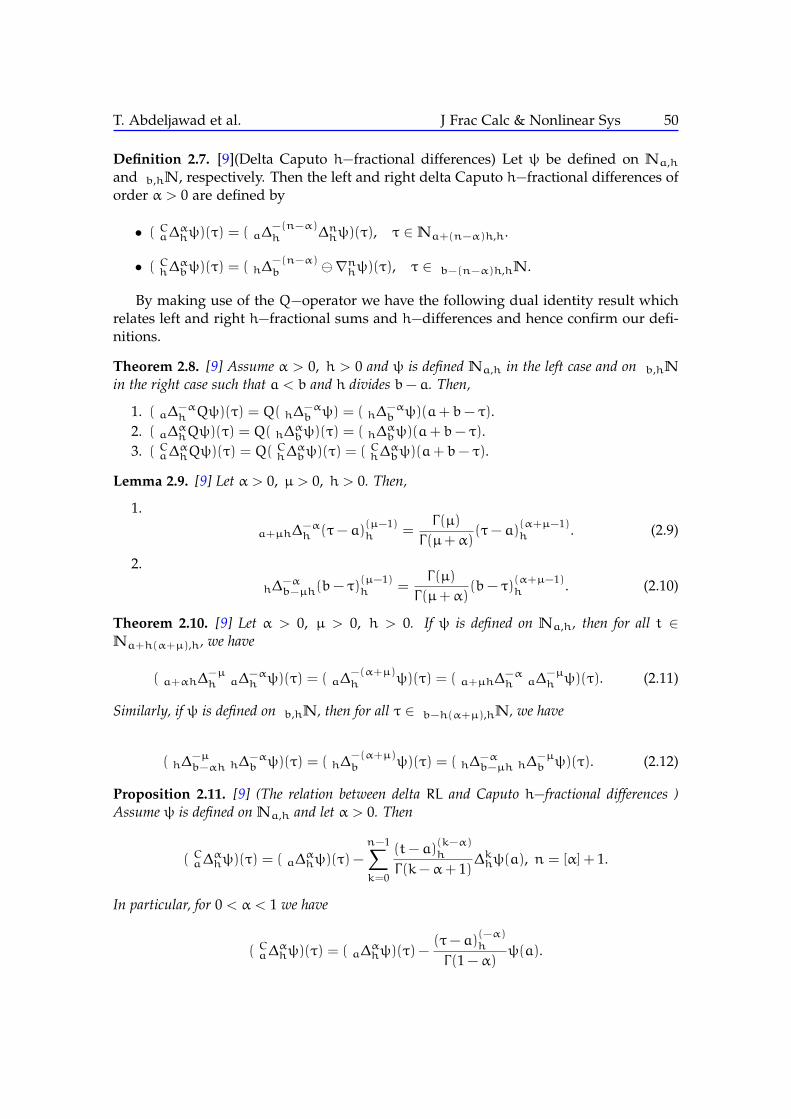
Definition 2.7. [9](Delta Caputo h−fractional differences) Let ψ be defined on Na,hand b,hN, respectively. Then the left and right delta Caputo h−fractional differences oforder α > 0 are defined by

• ( Ca∆αhψ)(τ) = ( a∆

−(n−α)h ∆nhψ)(τ), τ ∈Na+(n−α)h,h.

• ( Ch∆αbψ)(τ) = ( h∆

−(n−α)b ∇nhψ)(τ), τ ∈ b−(n−α)h,hN.

By making use of the Q−operator we have the following dual identity result whichrelates left and right h−fractional sums and h−differences and hence confirm our defi-nitions.

Theorem 2.8. [9] Assume α > 0, h > 0 and ψ is defined Na,h in the left case and on b,hN

in the right case such that a < b and h divides b− a. Then,

1. ( a∆−αh Qψ)(τ) = Q( h∆

−αb ψ) = ( h∆

−αb ψ)(a+ b− τ).

2. ( a∆αhQψ)(τ) = Q( h∆

αbψ)(τ) = ( h∆

αbψ)(a+ b− τ).

3. ( Ca∆αhQψ)(τ) = Q( Ch∆

αbψ)(τ) = ( Ch∆

αbψ)(a+ b− τ).

Lemma 2.9. [9] Let α > 0, µ > 0, h > 0. Then,

1.

a+µh∆−αh (τ− a)

(µ−1)h =

Γ(µ)

Γ(µ+α)(τ− a)

(α+µ−1)h . (2.9)

2.

h∆−αb−µh(b− τ)

(µ−1)h =

Γ(µ)

Γ(µ+α)(b− τ)

(α+µ−1)h . (2.10)

Theorem 2.10. [9] Let α > 0, µ > 0, h > 0. If ψ is defined on Na,h, then for all t ∈Na+h(α+µ),h, we have

( a+αh∆−µh a∆

−αh ψ)(τ) = ( a∆

−(α+µ)h ψ)(τ) = ( a+µh∆

−αh a∆

−µh ψ)(τ). (2.11)

Similarly, if ψ is defined on b,hN, then for all τ ∈ b−h(α+µ),hN, we have

( h∆−µb−αh h∆

−αb ψ)(τ) = ( h∆

−(α+µ)b ψ)(τ) = ( h∆

−αb−µh h∆

−µb ψ)(τ). (2.12)

Proposition 2.11. [9] (The relation between delta RL and Caputo h−fractional differences )Assume ψ is defined on Na,h and let α > 0. Then

( Ca∆αhψ)(τ) = ( a∆

αhψ)(τ) −

n−1∑k=0

(t− a)(k−α)h

Γ(k−α+ 1)∆khψ(a), n = [α] + 1.

In particular, for 0 < α < 1 we have

( Ca∆αhψ)(τ) = ( a∆

αhψ)(τ) −

(τ− a)(−α)h

Γ(1 −α)ψ(a).

T. Abdeljawad et al. J Frac Calc & Nonlinear Sys 51

On the other hand if ψ is defined on b,hN then

( Ch∆αbψ)(τ) = ( h∆

αbψ)(τ) −

n−1∑k=0

(b− τ)(k−α)h

Γ(k−α+ 1)∇khψ(b), n = [α] + 1.

In particular, for 0 < α < 1 we have

( Ch∆αbψ)(τ) = ( h∆

αbψ)(τ) −

(b− τ)(−α)h

Γ(1 −α)ψ(b).

Proposition 2.12. [9] For α > 0, h > 0 and ψ defined on Na,h we have for t ∈Na+nh,h ⊂Na,h

( a+αh∆αh a∆

−αh ψ)(τ) = ψ(τ) (2.13)

and( a+(n−α)h−h∆

−αh a∆

αhψ)(τ) = ψ(τ), α /∈N, (2.14)

( a∆−αh a∆

αhψ)(τ) = ψ(τ) −

n−1∑k=0

(τ− a)(k)h

k!∆khψ(a), α ∈N, (2.15)

where n = [α] + 1.

Proposition 2.13. [9] For α > 0, h > 0 andψ defined on b,hN, we have for t ∈ b−nh,hN ⊂b,hN

( h∆αb−αh h∆

−αb ψ)(τ) = ψ(τ) (2.16)

and( h∆

−αb−(n−α)h+h h∆

αbψ)(τ) = ψ(τ), α /∈N, (2.17)

( h∆−αb h∆

αbψ)(τ) = ψ(τ) −

n−1∑k=0

(b− τ)(k)h

k!∇khψ(b), α ∈N. (2.18)

Lemma 2.14. [9] For any α > 0 we have

( a∆−αh ∆hψ)(τ) = (∆h a∆

−αh ψ)(t) −

(τ− a)(α−1)h

Γ(α)ψ(a), (2.19)

where ψ is defined on Na,h. On the other hand, if ψ is defined on b,hN, then

( h∆−αb (−∇h)ψ)(τ) = (−∇h h∆−α

b ψ)(τ) −(b− τ)

(α−1)h

Γ(α)ψ(b). (2.20)

Similar to Theorem 4.10 in [18] and by the help of (2.19) and the observation that

a∆−(1−α)h ψ(τ) |τ=a+(1−α)h= h

1−αψ(a),

we can state the following delta discrete fractional Leibniz rule in the sense of Riemann-Liouville.

T. Abdeljawad et al. J Frac Calc & Nonlinear Sys 52

Lemma 2.15. For ψ defined on Na,h, h > 0 and 0 < α 6 1, we have the following identity.

a+(1−α)h∆−αh a∆

αhψ(τ) = ψ(τ) − h

1−α (t− a− (1 −α)h)(α−1)h ψ(a)

Γ(α). (2.21)

Proposition 2.16. Assume that α > 0, h > 0 andψ is defined on Na,h and b,hN, respectively.Then

( a+(n−α)h∆−αh

Ca∆

αhψ)(τ) = ψ(τ) −

n−1∑k=0

(τ− a)(k)h

k!∆khψ(a) (2.22)

and

( h∆−αb−(n−α)h

Ch∆

αbψ)(τ) = ψ(τ) −

n−1∑k=0

(b− τ)(k)h

k!∇khψ(a). (2.23)

2.3. The nabla fractional sums and differences on the isolated time scaleIn this part, we borrow our notations and their related basics from [9].

Definition 2.17. (Nabla h−fractional sums) Let ρ(τ) = τ− h, h > 0 be backward jumpoperator. Then, for a function f : Na,h = {a,a + h,a + 2h, . . .} → R, the nabla lefth−fractional sum of order α > 0 is given by

(a∇−αh f)(τ) =

1Γ(α)

∫τa

(τ− ρh(s))α−1h f(s)∇h

=1Γ(α)

τ/h∑k=a/h+1

(τ− ρh(kh))α−1h f(kh)h, t ∈Na+h,h.

The nabla right h−fractional sum of order α > 0 (ending at b)for f : b,hN = {b,b−h,b− 2h, . . .}→ R is written as

(h∇−αb f)(τ) =

1Γ(α)

∫bτ

(s− ρh(τ))α−1h f(s)∆hs =

1Γ(α)

b/h−1∑k=τ/h

(kh− ρh(τ))α−1h f(kh)h.

Definition 2.18. (Nabla h−RL fractional differences) The nabla left h−fractional differenceof order α > 0 (starting from a) has the form

(a∇αhf)(τ) = (∇nh a∇−(n−α)h f)(τ)

=∇nh

Γ(n−α)

τ∑k=a/h+1

(τ− ρh(kh))n−α−1h f(kh)h, τ ∈Na+h,h

and the nabla right h−fractional difference of order α > 0 (ending at b) is defined as

(h∇αbf)(τ) = (∆nhh∇−(n−α)b f)(τ)

=∆nh

Γ(n−α)

b/h−1∑k=τ

(kh− ρh(τ))n−α−1h f(kh)h, τ ∈ b−h,hN.

T. Abdeljawad et al. J Frac Calc & Nonlinear Sys 53

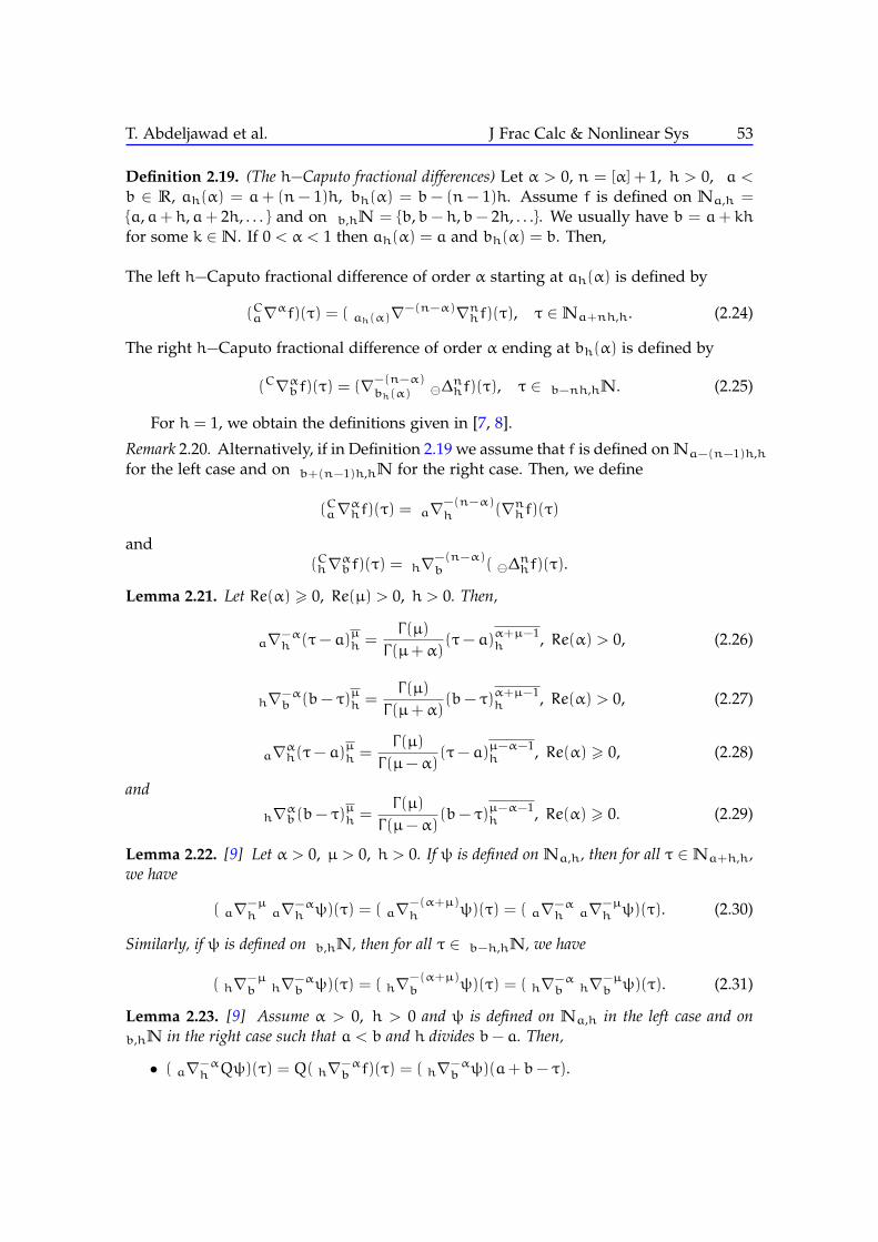
Definition 2.19. (The h−Caputo fractional differences) Let α > 0, n = [α] + 1, h > 0, a <

b ∈ R, ah(α) = a+ (n− 1)h, bh(α) = b− (n− 1)h. Assume f is defined on Na,h ={a,a+ h,a+ 2h, . . . } and on b,hN = {b,b− h,b− 2h, . . .}. We usually have b = a+ khfor some k ∈N. If 0 < α < 1 then ah(α) = a and bh(α) = b. Then,

The left h−Caputo fractional difference of order α starting at ah(α) is defined by

(Ca∇αf)(τ) = ( ah(α)∇−(n−α)∇nhf)(τ), τ ∈Na+nh,h. (2.24)

The right h−Caputo fractional difference of order α ending at bh(α) is defined by

(C∇αbf)(τ) = (∇−(n−α)bh(α) ∆

nhf)(τ), τ ∈ b−nh,hN. (2.25)

For h = 1, we obtain the definitions given in [7, 8].

Remark 2.20. Alternatively, if in Definition 2.19 we assume that f is defined on Na−(n−1)h,hfor the left case and on b+(n−1)h,hN for the right case. Then, we define

(Ca∇αhf)(τ) = a∇−(n−α)h (∇nhf)(τ)

and(Ch∇αbf)(τ) = h∇

−(n−α)b ( ∆

nhf)(τ).

Lemma 2.21. Let Re(α) > 0, Re(µ) > 0, h > 0. Then,

a∇−αh (τ− a)µh =

Γ(µ)

Γ(µ+α)(τ− a)α+µ−1

h , Re(α) > 0, (2.26)

h∇−αb (b− τ)µh =

Γ(µ)

Γ(µ+α)(b− τ)α+µ−1

h , Re(α) > 0, (2.27)

a∇αh(τ− a)µh =

Γ(µ)

Γ(µ−α)(τ− a)µ−α−1

h , Re(α) > 0, (2.28)

and

h∇αb(b− τ)µh =

Γ(µ)

Γ(µ−α)(b− τ)µ−α−1

h , Re(α) > 0. (2.29)

Lemma 2.22. [9] Let α > 0, µ > 0, h > 0. If ψ is defined on Na,h, then for all τ ∈Na+h,h,we have

( a∇−µh a∇−α

h ψ)(τ) = ( a∇−(α+µ)h ψ)(τ) = ( a∇−α

h a∇−µh ψ)(τ). (2.30)

Similarly, if ψ is defined on b,hN, then for all τ ∈ b−h,hN, we have

( h∇−µb h∇−α

b ψ)(τ) = ( h∇−(α+µ)b ψ)(τ) = ( h∇−α

b h∇−µb ψ)(τ). (2.31)

Lemma 2.23. [9] Assume α > 0, h > 0 and ψ is defined on Na,h in the left case and onb,hN in the right case such that a < b and h divides b− a. Then,

• ( a∇−αh Qψ)(τ) = Q( h∇−α

b f)(τ) = ( h∇−αb ψ)(a+ b− τ).

T. Abdeljawad et al. J Frac Calc & Nonlinear Sys 54

• ( a∇αhQψ)(τ) = Q( h∇αbψ)(τ) = ( h∇αbψ)(a+ b− τ).

• ( Ca∇αhQψ)(τ) = Q( Ch∇αbψ)(τ) = ( Ch∇αbψ)(a+ b− τ).

Lemma 2.24. (Nabla Leibniz for left Caputo fractional differences) Assume α,h > 0 and ξ isdefined on a suitable domain Na−(n−1)h, n = [α] + 1. Then,

( a∇−αh

Ca∇αhψ)(τ) = ψ(τ) −

n−1∑k=0

(τ− a)khk!

∇khψ(a). (2.32)

Alternatively, above we can define on Na and obtain the following form of Leibniz

( ah(α)∇−αh

Cah(α)

∇αhψ)(τ) = ψ(τ) −n−1∑k=0

(τ− a)khk!

∇khψ(a), (2.33)

where ah(α) = a+ (n− 1)h.

Lemma 2.25. (Nabla Leibniz for left Caputo fractional differences) Assume α,h > 0 and ψ isdefined on a suitable domain Na−(n−1)h, n = [α] + 1. Then,

( a∇−αh

Ca∇αhψ)(τ) = ψ(τ) −

n−1∑k=0

(t− a)khk!

∇khψ(a). (2.34)

Alternatively, above we can define ψ on Na and obtain the following form of Leibniz

( ah(α)∇−αh

Cah(α)

∇αhψ)(τ) = ψ(τ) −n−1∑k=0

(t− ah(α))kh

k!∇khψ(ah(α)), (2.35)

where ah(α) = a+ (n− 1)h.

Lemma 2.26. (Nabla Leibniz for right Caputo fractional differences) Assume α,h > 0 and ψ isdefined on a suitable domain b+(n−1)hN, n = [α] + 1. Then,

( h∇−αb

Ch∇αbψ)(τ) = ψ(τ) −

n−1∑k=0

(τ− a)khk!

∆khψ(b). (2.36)

Alternatively, above we can define ψ on b−(n−1)hN and obtain the following formof Leibniz rule

( bh(α)∇−αh

Cbh(α)

∇αhψ)(τ) = ψ(τ) −n−1∑k=0

(bh(α) − t)kh

k!∆khψ(bh(α)), (2.37)

where bh(α) = b− (n− 1)h.If we let ρ = 1 in Proposition 5.1 of [11] we obtain the following essential tool lemma.

T. Abdeljawad et al. J Frac Calc & Nonlinear Sys 55

Lemma 2.27. For any α ∈ C with Re(α) > 0 , n = [Re(α)] + 1 and f defined on a suitabledomain, we have

( Ca∇αhf)(τ) = ( a∇αhf)(τ) −n−1∑k=0

(τ− a)k−αh

Γ(k+ 1 −α)(∇khf)(a). (2.38)

Similarly, by applying the Q−operator, we have

( Ch∇αbf)(τ) = ( h∇αbf)(τ) −n−1∑k=0

(b− t)k−αh

Γ(k+ 1 −α)( ∆

khf)(b), (2.39)

where ∆kh = (−1)k∆kh.

3. Weighted left and right fractional sums and differences

3.1. In the nabla settingDefinition 3.1. (Left weighted fractional sums into nabla) The left nabla weighted frac-tional sum of a function η defined on Na,h = {a,a + h,a + 2h, ...} via a function ω

defined on Na,h of order α, Re(α) > 0 and starts at a, is defined by

( a∇−αω,hη)(t) =

1ω(t)

a∇−αh [ω(t)η(t)] =

1ω(t)Γ(α)

∫ta

(t− ρh(s))α−1h ω(s)η(s)∇hs. (3.1)

Definition 3.2. (Left weighted fractional difference into nabla) The left nabla weightedfractional difference of a function η defined on Na,h = {a,a+h,a+ 2h, ...} via a functionω defined on Na,h of order α, Re(α) > 0 and starts at a, is defined by

( a∇αω,hη)(t) =1

ω(t)a∇αh[ω(t)η(t)] =

1ω(t)Γ(−α)

∫ta

(t− ρh(s))−α−1h ω(s)η(s)∇hs.

(3.2)

Next, as usual, we give the definitions in the right case so that it can be verified bythe role of summation by parts.

Definition 3.3. (Right weighted fractional sums into nabla) The right nabla weightedfractional sum of a function η defined on b,hN = {b,b− h,a− 2h, ...} via a function ωdefined on b,hN of order α, Re(α) > 0 and ends at b, is defined by

( ω,h∇−αb η)(t) = ω(t) h∇−α

b [ω−1(t)η(t)] =ω(t)

Γ(α)

∫bt

(s− ρh(t))α−1h ω−1(s)η(s)∆hs.

(3.3)

Definition 3.4. (Right weighted fractional difference into nabla) The right nabla weightedfractional difference of a function η defined on b,hN = {b,b−h,a− 2h, ...} via a functionω defined on b,hN of order α, Re(α) > 0 and ends at b, is defined by

( ω,h∇αbη)(t) = ω(t) h∇αb [ω−1(t)η(t)] =ω(t)

Γ(−α)

∫bt

(s− ρh(t))−α−1h ω−1(s)η(s)∆hs.

(3.4)

T. Abdeljawad et al. J Frac Calc & Nonlinear Sys 56

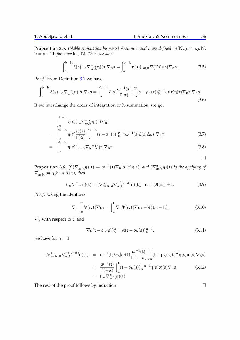
Proposition 3.5. (Nabla summation by parts) Assume η and ξ are defined on Na,h ∩ b,hN,b = a+ kh for some k ∈N. Then, we have∫b−h

a

ξ(s)( a∇−αω,hη)(s)∇hs =

∫b−ha

η(s)( ω,h∇−αb ξ)(s)∇hs. (3.5)

Proof. From Definition 3.1 we have∫b−ha

ξ(s)( a∇−αω,hη)(s)∇hs =

∫b−ha

ξ(s)ω−1(s)

Γ(α)[

∫sa

(s− ρh(r))α−1h ω(r)η(r)∇hr]∇hs.

(3.6)If we interchange the order of integration or h-summation, we get

∫b−ha

ξ(s)( a∇−αω,hη)(s)∇hs

=

∫b−ha

η(r)ω(r)

Γ(α)[

∫b−hr

(s− ρh(r))α−1h ω−1(s)ξ(s)∆hs]∇hr (3.7)

=

∫b−ha

η(r)( ω,h∇−αb ξ)(r)∇hr. (3.8)

Proposition 3.6. If (∇1ω,hη)(t) = ω−1(t)∇h[ω(t)η(t)] and (∇nω,hη)(t) is the applying of

∇1ω,h on η for n times, then

( a∇αω,hη)(t) = (∇nω,h a∇−(n−α)ω,h η)(t), n = [<(α)] + 1. (3.9)

Proof. Using the identities

∇h∫ta

Ψ(s, t)∇hs =∫ta

∇hΨ(s, t)∇hs−Ψ(t, t− h), (3.10)

∇h with respect to t, and

∇h(t− ρh(s))αh = α(t− ρh(s))α−1h , (3.11)

we have for n = 1

(∇1ω,h a∇

−(n−α)ω,h η)(t) = ω−1(t)∇h[ω(t)

ω−1(t)

Γ(1 −α)

∫ta

(t− ρh(s))−αh η(s)ω(s)∇hs]

=ω−1(t)

Γ(−α)

∫ta

(t− ρh(s))−α−1h η(s)ω(s)∇hs (3.12)

= ( a∇αω,hη)(t).

The rest of the proof follows by induction.

T. Abdeljawad et al. J Frac Calc & Nonlinear Sys 57

Proposition 3.7. If (∇1ω,hη)(t) = −ω(t)∆h[ω

−1(t)η(t)] and (∇nω,hη)(t) is the applying of

∇1ω,h on η for n times, then

( ω,h∇αbη)(t) = (∇nω,h ω,h∇

−(n−α)b η)(t), n = [<(α)] + 1. (3.13)

Proof. The proof is similar to that in Proposition 3.30 and follows by the identities

∆h

∫bt

Ψ(s, t)∆hs =∫bt

∆hΨ(s, t)∆hs−Ψ(t, t+ h), (3.14)

∆h with respect to t, and

∆h(s− ρh(t))αh = −α(s− ρh(t))

α−1h . (3.15)

In fact, Proposition 3.5 is also valid when we replace α by −α. Hence, the followingintegration by parts is also valid.

Proposition 3.8. (Nabla by parts the weighted fractional differences) Assume η and ξ are definedon Na,h ∩ b,hN, b = a+ kh for some k ∈N. Then, we have∫b−h

a

ξ(s)( a∇αω,hη)(s)∇hs =∫b−ha

η(s)( ω,h∇αbξ)(s)∇hs. (3.16)

Alternatively, we can define them by verifying via the action of the Q-operator whichis defined by Qη(t) = η(a+ b− t).

Definition 3.9. (Q-Right weighted fractional sums into nabla) The left nabla weightedfractional sum of a function η defined on b,hN = {b,b− h,a− 2h, ...} via a function ωdefined on b,hN of order α, Re(α) > 0 and ends at b, is defined by

( Qω,h∇−αb η)(t) =

1(Qω)(t)

h∇−αb [(Qω)(t)η(t)]

=1

(Qω)(t)Γ(α)

∫bt

(s− ρh(t))α−1h (Qω)(s)η(s)∆hs. (3.17)

Definition 3.10. (Q-Right weighted fractional difference into nabla) The right nablaweighted fractional difference of a function η defined on b,hN = {b,b − h,a − 2h, ...}via a function ω defined on b,hN of order α, Re(α) > 0 and ends at b, is defined by

( Qω,h∇αbη)(t) =

1(Qω)(t)

h∇αb [(Qω)(t)η(t)]

=1

(Qω)(t)Γ(−α)

∫bt

(s− ρh(t))−α−1h (Qω)(s)η(s)∆hs. (3.18)

Remark 3.11. The weighted fractional sums and differences have the following proper-ties:

T. Abdeljawad et al. J Frac Calc & Nonlinear Sys 58

1. If ω satisfies ω(t)ω(a+ b− t) = 1, the weighted fractional sums and differencesdefined in by the verification of by parts coincide with the corresponding Q−ones.In particular, it is the case when ω(t) = 1, which gives the classical discrete frac-tional operators. Another example, when ω(t) = t

b−t and a = 0. Notice that, thisω(t) is strictly increasing on b−h,hN.

2. The following Q−relations are valid:

• Q( a∇−αω,hη)(t) = ( Qω,h∇

−αb Qη)(t).

• Q( a∇αω,hη)(t) = ( Qω,h∇αbQη)(t).

• ( a∇−µω,h a∇

−αω,hη)(t) = a∇−(α+µ)

ω,h η(t).

• ( ω,h∇−αb ω,h∇−µ

b η)(t) = ω,h∇−(α+µ)b η(t).

• ( Qω,h∇−αb

Qω,h∇

−µb η)(t) = Q

ω,h∇−(α+µ)b η(t), provided that

ω(t)ω(a+ b− t) = 1. (3.19)

3. If the weighted function ω(t) satisfies the following tempered type conditions(a) ω(t+ s) = ω(t)ω(s)(b) ω(−t) = ω−1(t) and ω−1(−t) = ω(t),

then, we have

• ( a∇−αω,hQψ)(t) = Q( ω,h∇−α

b f)(t) = ( ω,h∇−αb ψ)(a+ b− t).

• ( a∇αω,hQψ)(t) = Q( ω,h∇αbf)(t) = ( ω,h∇αbψ)(a+ b− t).

• ( Ca∇αω,hQψ)(t) = Q( Cω,h∇αbf)(t) = ( Cω,h∇αbψ)(a+ b− t).The proof can be done by definition and Lemma 2.23. For example, to prove thefirst part, by the help of the first part of Lemma 2.23 and the properties of ω(t),we have

Q( ω,h∇−αb ψ)(t) = Q

[ω(t) h∇−α

b

(ω−1(t)ψ(t)

)]= ω(a+ b− t) a∇−α

h

(ω−1(a+ b− t)ψ(a+ b− t)

)= ω(a)ω(b)ω(−t)ω−1(a)ω−1(b) a∇−α

h

(ω−1(−t)Qψ(t)

)= ω−1(t) a∇−α

h

(ω1(t)Qψ(t)

)= ( a∇−α

ω,hQψ)(t).

The proof the other parts is similar. However, in the proof of the second part, wemake use of the second part of Lemma 2.23 and the third part by making use ofthe third part of Lemma 2.23.

Above, we called this weighted by tempered type, since we can choose ω(t) the nablaexponential function and ω−1(t) its minus circle exponential function [16].

Theorem 3.12. (The semi-group property for tempered sums) Let α > 0, µ > 0, h > 0. If ψ isdefined on Na,h, then for all t ∈Na+h,h, we have

( a∇−µω,h a∇

−αω,hψ)(t) = ( a∇−(α+µ)

ω,h ψ)(t) = ( a∇−αω,h a∇

−µω,hψ)(t). (3.20)

T. Abdeljawad et al. J Frac Calc & Nonlinear Sys 59

Similarly, if ψ is defined on b,hN, then for all t ∈ b−h,hN, we have

( ω,h∇−µb ω,h∇−α

b ψ)(t) = ( ω,h∇−(α+µ)b ψ)(t) = ( ω,h∇−α

b ω,h∇−µb ψ)(t). (3.21)

Proof. By the help of Lemma 2.22, we have

( a∇−µω,h a∇

−αω,hψ)(t) = ω−1(t) a∇−µ

ω,h[ω(t) a∇−αω,hψ(t)]

= ω−1(t) a∇−µω,h(ω(t)ω−1(t)

× a∇−αh [ω(t)ψ(t)])

= ω−1(t) a∇−µω,h( a∇

−αh [ω(t)ψ(t)])

= ω−1(t) a∇−(α+µ)h [ω(t)ψ(t)]

= ( a∇−(α+µ)ω,h ψ)(t).

The proof of (3.21) is similar.

3.2. In the delta settingDefinition 3.13. (Left weighted fractional sums into delta) The left delat weighted frac-tional sum of a function η defined on Na,h = {a,a + h,a + 2h, ...} via a function ω

defined on Na,h of order α, Re(α) > 0 and starts at a, is defined by

( a∆−αω,hη)(t) =

1ω(t)

a∆−αh [ω(t)η(t)]

=1

ω(t)Γ(α)

∫σh(t−αh)a

(t− σh(s))(α−1)h ω(s)η(s)∆hs, t ∈Na+αh,h.(3.22)

Definition 3.14. (Left weighted fractional difference into delta) The left delta weightedfractional difference of a function η defined on Na,h = {a,a+h,a+ 2h, ...} via a functionω defined on Na,h of order α, Re(α) > 0 and starts at a, is defined by

( a∆αω,hη)(t) =

1ω(t)

a∆αh[ω(t)η(t)]

=1

ω(t)Γ(−α)

∫σh(t−αh)a

(t− σh(s))(−α−1)h ω(s)η(s)∆hs, (3.23)

where t ∈Na+(n−α)h,h.

Definition 3.15. (Right weighted fractional sums into delta) The right delta weightedfractional sum of a function η defined on b,hN = {b,b− h,a− 2h, ...} via a function ωdefined on b,hN of order α, Re(α) > 0 and ends at b, is defined by

( ω,h∆−αb η)(t) = ω(t) h∆

−αb [ω−1(t)η(t)]

=ω(t)

Γ(α)

∫bρh(t+αh)

(s− σh(t))(α−1)h ω−1(s)η(s)∇hs, (3.24)

where t ∈ b−αh,hN.

T. Abdeljawad et al. J Frac Calc & Nonlinear Sys 60

Definition 3.16. (Right weighted fractional difference into delta) The right delta weightedfractional difference of a function η defined on b,hN = {b,b−h,a− 2h, ...} via a functionω defined on b,hN of order α, Re(α) > 0 and ends at b, is defined by

( ω,h∆αbη)(t) = ω(t) h∆

αb [ω

−1(t)η(t)]

=ω(t)

Γ(−α)

∫bρh(t+αh)

(s− σh(t))(−α−1)h ω−1(s)η(s)∇hs, (3.25)

where t ∈ b−(n−α)h,hN.

Remark 3.17. For ω(t) = t in Definition 3.13 and Definition 3.15, we get the definitionsin Section 1.3 in [9].

The following fractional summation by parts is a modification of Proposition 4.5 in[8] to h−step and under a weight function.

Proposition 3.18. (Delta summation by parts) Assume η and ξ are defined on Na,h ∩ b,hN,b = a+ kh for some k ∈N. Then, we have∫b

a+hξ(s)( a+h∆

−αω,hη)(s+αh)∆hs =

∫ba+h

η(s)( ω,h∆−αb−hξ)(s−αh)∆hs. (3.26)

Proof. The proof is similar to that in Proposition 3.5 and follows by definition, inter-changing the order of h-summations and by noting that s − σh(r − αh) = s + αh −σh(r).

Proposition 3.19. If (∆1ω,hη)(t) = ω−1(t)∆h[ω(t)η(t)] and (∆nω,hη)(t) is the applying of

∆1ω,h on η for n times, then

( a∆αω,hη)(t) = (∆nω,h a∆

−(n−α)ω,h η)(t), n = [<(α)] + 1. (3.27)

Proof. The proof is similar to that in Proposition 3.7. In fact, it follows by employing theidentities Using the identities

∆h

∫t+αha

Ψ(s, t)∆hs =∫t+αh+ha

∆hΨ(s, t)∆hs+Ψ(t+αh, t+ h), t ∈Na+(1−α)h,h,

(3.28)∇h with respect to t, and

∆h(t− σh(s))(α)h = α(t− σh(s))

(α−1)h . (3.29)

Proposition 3.20. If (∆1ω,hη)(t) = −ω(t)∇h[ω−1(t)η(t)] and (∆n

ω,hη)(t) is the applying of∆1ω,h on η for n times, then

( ω,h∆αbη)(t) = (∆n

ω,h ω,h∆−(n−α)b η)(t), n = [<(α)] + 1. (3.30)

T. Abdeljawad et al. J Frac Calc & Nonlinear Sys 61

Proof. The proof is similar to that in Proposition 3.19 and follows by the identities

∇h∫bt−αh

Ψ(s, t)∇hs =∫bt−αh

∇hΨ(s, t)∇hs−Ψ(t−αh, t), (3.31)

∇h with respect to t, and

∇h(s− σh(t))(α)h = −α(s− σh(t))

(α−1)h . (3.32)

In fact, Proposition 3.18 is also valid when we replace α by −α. Hence, the followingintegration by parts is also valid.

Proposition 3.21. (Delta by parts of the weighted fractional differences) Assume η and ξ aredefined on Na,h ∩ b,hN, b = a+ kh for some k ∈N. Then, we have∫b

a+hξ(s)( a+h∆

αω,hη)(s−αh)∆hs =

∫ba+h

η(s)( ω,h∆αb−hξ)(s+αh)∆hs. (3.33)

Remark 3.22. The same steps can be carried to the delta case as done in Definition 3.9,Definition 3.10 and in Remark 3.11. However, nabla will be replaced by delta and theaction of the Q−operator for delta fractional sums and differences will be used. Also,we have to care about the domain of the delta defined fractional difference and sumoperators.

4. The weighted Caputo fractional differences and sums

4.1. In the nabla settingDefinition 4.1. (The weighted h−Caputo fractional differences) Let α > 0, n = [α] + 1, h >0, a < b ∈ R, and assume f and ω are defined on Na−(n−1)h,h for the left case and onb+(n−1)h,hN for the right case. Then the left weighted h−Caputo fractional differenceof order α starting at a and via ω is defined by

(Ca∇αω,hf)(t) = a∇−(n−α)ω,h (∇nω,hf)(t),

and the right one ending at b by

(Cω,h∇αbf)(t) = ω,h∇−(n−α)b (∇n

ω,hf)(t),

where (∇nω,hη(t)) is the application of (∇1ω,hη)(t) = ω

−1(t)∇h[ω(t)η(t)] n− times,and (∇n

ω,hη)(t) is the application of (∇1ω,hη)(t) = −ω(t)∆h[ω

−1(t)η(t)], n− times.

For h = 1,ω(t) = 1, we obtain the definitions given in [7, 8].

T. Abdeljawad et al. J Frac Calc & Nonlinear Sys 62

Remark 4.2. Alternatively, if in Definition 4.1 we assume that f is defined on Na−(n−1)h,hfor the left case and on b+(n−1)h,hN for the right case, the weighted left and right h-Caputo differences via ω are defined by

(Ca∇αω,hf)(t) = ω−1(t) Ca∇αh[ω(t)f(t)], t ∈Na−h,h. (4.1)

The right ω−weighted h−Caputo fractional difference of order α ending at b is definedby

(Cω,h∇αbf)(t) = ω(t) Ch∇αb [ω−1(t)f(t)], t ∈ b−h,hN. (4.2)

This clear by splitting (∇nω,hη(t)) in the left case and (∇nω,hη(t)) in the right case.

Theorem 4.3. (The relation between weighted Riemann and Caputo types) For any α ∈ C, withRe(α) > 0 , n = [Re(α)] + 1 and ξ, ω defined on a suitable domain, we have

( Ca∇αω,hξ)(t) = ( a∇αω,hξ)(t) −ω−1(t) (4.3)

×n−1∑k=0

(t− a)k−αh

Γ(k+ 1 −α)(∇kh[ω(t)ξ(t)])(a).

Similarly, for the right case, we have

( Cω,h∇αbξ)(t) = ( ω,h∇αbξ)(t) (4.4)

− ω(t)

n−1∑k=0

(b− t)k−αh

Γ(k+ 1 −α)( ∆

kh[ω

−1(t)ξ(t)])(b).

Proof. In (2.38) set f(t) = ω(t)ξ(t) to get

( Ca∇αhω(t)ξ(t))(t) = ( a∇αh ω(t)ξ(t))(t) (4.5)

−

n−1∑k=0

(t− a)k−αh

Γ(k+ 1 −α)(∇kh[ω(t)ξ(t)])(a).

The multiplication of (4.5) by ω−1(t) will imply that

( Ca∇αω,hξ(t))(t) = ( a∇αω,hξ)(t) (4.6)

− ω−1(t)

n−1∑k=0

(t− a)k−αh

Γ(k+ 1 −α)(∇kh[ω(t)ξ(t)])

To prove the right case set f(t) = ω−1(t)ξ(t) in (2.39) and then multiply by ω(t).

T. Abdeljawad et al. J Frac Calc & Nonlinear Sys 63

4.2. In the delta settingDefinition 4.4. (Left weighted Caputo fractional difference into delta) The left deltaweighted fractional difference of a function η defined on Na,h = {a,a+h,a+ 2h, ...} viaa function ω defined on Na,h of order α, Re(α) > 0 and starts at a, is defined by

( Ca∆αω,hη)(t) =

1ω(t)

Ca∆

αh[ω(t)η(t)], (4.7)

where t ∈Na+(n−α)h,h and Ca∆

αh is the delta Caputo fractional difference.

Definition 4.5. (Right Caputo weighted fractional differences into delta) The right deltaweighted fractional sum of a function η defined on b,hN = {b,b− h,a− 2h, ...} via afunction ω defined on b,hN of order α, Re(α) > 0 and ends at b, is defined by

( Cω,h∆αbη)(t) = ω(t) Ch∆

αb [ω

−1(t)η(t)], (4.8)

where t ∈ b−(n−α)h,hN and Ch∆

αb is the right Caputo fractional difference.

Theorem 4.6. (The relation between weighted Riemann and Caputo types) For any α ∈ C withRe(α) > 0 , n = [Re(α)] + 1 and ξ, ω defined on a suitable domain, we have

( Ca∆αω,hξ)(t) = ( a∆

αω,hξ)(t) −ω

−1(t) (4.9)

×n−1∑k=0

(t− a)(k−α)h

Γ(k+ 1 −α)(∆kh[ω(t)ξ(t)])(a).

Similarly, for the right case, we have

( Cω,h∆αbξ)(t) = ( ω,h∆

αbξ)(t) (4.10)

− ω(t)

n−1∑k=0

(b− t)(k−α)h

Γ(k+ 1 −α)( ∇kh[ω−1(t)ξ(t)])(b).

Proof. In Proposition 2.11 set f(t) = ω(t)ξ(t) to get

( Ca∆αhω(t)ξ(t))(t) = ( a∆

αhω(t)ξ(t))(t) (4.11)

−

n−1∑k=0

(t− a)k−αh

Γ(k+ 1 −α)(∆kh[ω(t))ξ(t)])(a).

The multiplication of (4.11) by ω−1(t) will imply that

( Ca∆αω,hξ(t))(t) = ( a∆

αω,hξ)(t) (4.12)

− ω−1(t)

n−1∑k=0

(t− a)(k−α)h

Γ(k+ 1 −α)(∆kh[ω(t)ξ(t)])

To prove the right case set f(t) = ω−1(t)ξ(t) in the right identity in Proposition 2.11 andthen multiply by ω(t).

T. Abdeljawad et al. J Frac Calc & Nonlinear Sys 64

5. The Leibniz type rules

This section provides the tool to transform fractional for nabla and delta weighteddifference equations to summation equations so that the method of successive approxi-mation can be applied.

The first theorem is dealing with the Caputo case in the nabla setting.

Theorem 5.1. (The application of the sum on the Caputo weighted difference- Leibniz Rule)Assume α,h > 0 and ξ, ω are defined on Na−(n−1)h,h in the left case and on b+(n−1)h,hN

in the right case. Then, we have

a∇−αω,h

Ca∇αω,hξ(t) =

[ξ(t) −ω−1(t)

n−1∑k=0

(t− a)khk!

(∇khω(t)ξ(t)

)(a)

], (5.1)

and

ω,h∇−αb

Cω,h∇αbξ(t) =

[ξ(t) −ω(t)

n−1∑k=0

(b− t)khk!

((∆

khω

−1(t)ξ(t)))(b)

]. (5.2)

In particular, if 0 < α 6 1, we have

a∇−αω,h

Ca∇αω,hξ(t) = ξ(t) −ω

−1(t)ω(a)ξ(a), (5.3)

andω,h∇−α

b ω,h∇αbξ(t) = ξ(t) − ω(t)ω−1(b)ξ(b). (5.4)

Proof. Using the ω−weighted fractional sum and Caputo difference definitions and byapplying the Leibniz rule (2.34), we obtain

a∇−αω,h

Ca∇αω,hξ(t) = ω−1(t) a∇−α

h

[ω(t) Ca∇αω,hξ(t)

]= ω−1(t) a∇−α

h

[ω(t)ω−1(t) Ca∇αh(ω(t)ξ(t))

]= ω−1(t) a∇−α

hCa∇αh [ω(t)ξ(t)]

= ω−1(t)

[ω(t)ξ(t) −

n−1∑k=0

(t− a)khk!

(∇khω(t)ξ(t)

)(a)

]

=

[ξ(t) −ω−1(t)

n−1∑k=0

(t− a)khk!

(∇khω(t)ξ(t)

)(a)

]The right case is similar and can be proved by making use of (2.36).

Remark 5.2. Using the definitions and the fact that a∇−αh a∇αhξ(t) = ξ(t), it is straight-

forward to show that

a∇−αω,h a∇

αω,hξ(t) = ξ(t). (5.5)

Indeed, we have

T. Abdeljawad et al. J Frac Calc & Nonlinear Sys 65

a∇−αω,h a∇

αω,hξ(t) = ω−1(t) a∇−α

h [ω(t)( a∇αhξ)(t)]

= ω−1(t) a∇−αh [ω(t)ω−1(t)( a∇αhω(t)ξ)(t)]

= ω−1(t)ω(t)ξ(t)

= ξ(t).

Hence, it logical to generate fractional ω−weighted initial value difference equationsin the setting of Riemann by starting at a− 1. For example the following system is ofinterest

a−h∇αω,hξ(t) = f(t, x(t)), ξ(a) = c0, 0 < α 6 1, h > 0. (5.6)

For the h = 1, ω(t) = 1 case we refer to [8]. For the hZ case with ω(t) = 1 we refer to[12]. Indeed, in [12], for α ∈ (0, 1], it was proved that

a∇−αh a−h∇αhξ(t) = ξ(t) −

h1−α

Γ(α)(t− a+ h)α−1

h ξ(a). (5.7)

As a result of (5.7), it is straight froward to show that

a∇−αω,h a−h∇

αω,hξ(t) = ξ(t) −

h1−α

Γ(α)(t− a+ h)α−1

h ω−1(t)ω(a)ξ(a). (5.8)

The next theorem is about the delta Caputo weighted Leibniz rule whose proof issimilar to the nabla case and can be proved by the help of the delta Caputo Leibniz rulein the non-weighted case as stated in Proposition 2.16.

Theorem 5.3. (The application of the sum on the Caputo weighted difference- Leibniz Rule)Assume α,h > 0 and ξ, ω are defined on Na,h in the left case and on b,hN in the right case.Then, we have

a+(n−α)h∆−αω,h

Ca∆

αω,hξ(t) =

[ξ(t) −ω−1(t)

n−1∑k=0

(t− a)(k)h

k!(∆khω(t)ξ(t)

)(a)

], (5.9)

and

ω,h∆−αb−(n−α)h

Cω,h∆

αbξ(t) =

[ξ(t) −ω(t)

n−1∑k=0

(b− t)(k)h

k!((∇khω−1(t)ξ(t)

))(b)

].

(5.10)In particular, if 0 < α 6 1, we have

a+(n−α)h∇−αω,h

Ca∇αω,hξ(t) = ξ(t) −ω

−1(t)ω(a)ξ(a), (5.11)

andω,h∇−α

b−(n−α)hCω,h∇αbξ(t) = ξ(t) − ω(t)ω−1(b)ξ(b). (5.12)

T. Abdeljawad et al. J Frac Calc & Nonlinear Sys 66

Making use of Lemma 2.15, we can state the following Leinbniz rule in the frame ofRiemann-Lioulle.

Proposition 5.4. For α ∈ (0, 1], h > 0 and ξ define on Na,h, we have

a+(1−α)h∆−αω,h a∆

αω,hξ(t) = ψ(t) − h

1−α (t− a− (1 −α)h)(α−1)h ω(a)ω−1(t)ξ(a)

Γ(α).

(5.13)In particular, if ω(t) is of tempered type, then we have

a+(1−α)h∆−αω,h a∆

αω,hξ(t) = ψ(t) − h

1−α (t− a− (1 −α)h)(α−1)h ω−1(t− a)ξ(a)

Γ(α). (5.14)

6. More integration by parts

6.1. In the nabla settingThe following h-discrete tempered integration by parts are to interchange between

the Caputo and Riemann differences. In fact, by use the nabla integration by parts onthe hZ time scale [16]:

∫ba

f(t)∇hg(t)∇ht = f(t)g(t)|ba −∫ba

g(t− h)∇hf(t)∇ht, b− a = kh, k ∈N. (6.1)

Proposition 6.1. (Nabla by parts for the tempered fractional differences from left Caputo to rightRiemann ) Assume η and ξ are defined on Na,h ∩ b,hN, b = a+ kh for some k ∈ N. Then,we have∫b−h

a

ξ(s)( Ca∇αω,hη)(s)∇hs = η(s) ω,h∇−(1−α)b ξ(s) |b−ha (6.2)

+

∫b−2h

a−hη(s) ω,h∇αbξ(s)(s)∇sh

(6.3)

Proof. From Remark 4.2, Proposition 3.5 with ω(t) = 1, (6.1), and Definition 3.4 , weproceed by

T. Abdeljawad et al. J Frac Calc & Nonlinear Sys 67

∫b−ha

ξ(s)( Ca∇αω,hη)(s)∇hs

=

∫b−ha

ξ(s)ω−1(s) Ca∇αh(ω(s)η(s))∇hs

=

∫b−ha

ξ(s)ω−1(s) a∇−(1−α)h ∇h[ω(s)η(s)]∇hs

=

∫b−ha

h∇−(1−α)b [ω−1(s)ξ(s)]∇h[ω(s)η(s)]∇hs

= η(s)ω(s)∇−(1−α)b [ω−1(s)ξ(s)] |b−ha

−

∫b−ha

η(s− h)ω(s− h)∇h h∇−(1−α)b [ω−1(s)ξ(s)]∇hs

= η(s) ω,h∇−(1−α)b ξ(s) |b−ha

+

∫b−ha

η(s− h)ω(s− h)(−∆h) h∇−(1−α)b [ω−1(s)ξ(s)](s− h)∇hs

= η(s) ω,h∇−(1−α)b ξ(s) |b−ha

+

∫b−ha

η(s− h)ω(s− h) h∇αb [ω−1(s)ξ(s)](s− h)∇hs

= η(s) ω,h∇−(1−α)b ξ(s) |b−ha

+

∫b−2h

a−hη(s) ω,h∇αbξ(s)(s)∇sh

(6.4)

Remark 6.2. If we let ω(t) = 1 and h = 1 in Proposition 6.1, then we recover Theorem 43in [7].

In the next result, we use the following version of integration by parts [16]:

∫ba

fρ(t)∇hg(t)∇ht = f(t)g(t)|ba −∫ba

g(t)∇hf(t)∇ht, b− a = kh, k ∈N, (6.5)

where fρ(t) = f(t− h).

Proposition 6.3. (Nabla by parts for the tempered fractional differences from left Reimann toright Caputo ) Assume η and ξ are defined on Na,h ∩ b,hN, b = a+ kh for some k ∈ N.Then, we have∫b−h

a

ξ(s)( a∇αω,hη)(s)∇hs

= ω−1(s+ h) a∇−(1−α)h [η(s)ω(s)]ξ(s+ h) |b−ha

+

∫b−ha

η(s) Cω,h∇αbξ(s)∇sh. (6.6)

T. Abdeljawad et al. J Frac Calc & Nonlinear Sys 68

Proof. From Definition 3.2, (6.5), Proposition 3.5 with ω(t) = 1, and Remark 4.2, weproceed by

∫b−ha

ξ(s)( a∇αω,hη)(s)∇hs

=

∫b−ha

ξ(s)ω−1(s) a∇αh(ω(s)η(s))∇hs

=

∫b−ha

(ξσ)ρ(s)((ω−1)σ)ρ∇h a∇−(1−α)h [ω(s)η(s)]∇hs

= ω−1(s+ h) a∇−(1−α)h [η(s)ω(s)]ξ(s+ h) |b−ha

−

∫b−ha

a∇−(1−α)h [ω(s)η(s)]∇h[ξσ(s)(ω−1)σ(s)]∇sh

= ω−1(s+ h) a∇−(1−α)h [η(s)ω(s)]ξ(s+ h) |b−ha

−

∫b−ha

a∇−(1−α)h [ω(s)η(s)]∆h[ξ(s)ω

−1(s)]∇sh

= ω−1(s+ h) a∇−(1−α)h [η(s)ω(s)]ξ(s+ h) |b−ha

+

∫b−ha

η(s)ω(s) h∇−(1−α)b (−∆h)[ξ(s)ω

−1(s)]∇sh

= ω−1(s+ h) a∇−(1−α)h [η(s)ω(s)]ξ(s+ h) |b−ha

+

∫b−ha

η(s)ω(s) Ch∇αb [ξ(s)ω−1(s)]∇sh

= ω−1(s+ h) a∇−(1−α)h [η(s)ω(s)]ξ(s+ h) |b−ha

+

∫b−ha

η(s) Cω,h∇αbξ(s)∇sh

Remark 6.4. Other integration by parts can be formulated by changing the rule betweenω−weighted left and right and Rieman and Caputo settings. Also, all including theabove ones can be generalized for the higher order.

6.2. In the delta settingThe following h-discrete tempered integration by parts are to interchange between

the Caputo and Riemann differences. In fact, by use the nabla integration by parts onthe hZ time scale [15]:

∫ba

f(t)∆hg(t)∆ht = f(t)g(t)|ba −

∫ba

g(t+ h)∆hf(t)∆ht, b− a = kh, k ∈N. (6.7)

T. Abdeljawad et al. J Frac Calc & Nonlinear Sys 69

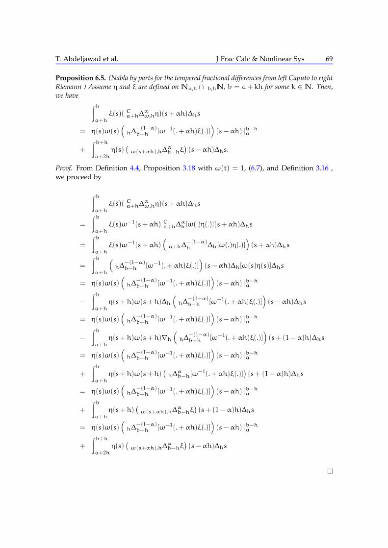
Proposition 6.5. (Nabla by parts for the tempered fractional differences from left Caputo to rightRiemann ) Assume η and ξ are defined on Na,h ∩ b,hN, b = a+ kh for some k ∈ N. Then,we have ∫b

a+hξ(s)( Ca+h∆

αω,hη)(s+αh)∆hs

= η(s)ω(s)(h∆

−(1−α)b−h [ω−1(. +αh)ξ(.)]

)(s−αh) |b−ha

+

∫b+ha+2h

η(s)(ω(s+αh),h∆

αb−hξ

)(s−αh)∆hs.

Proof. From Definition 4.4, Proposition 3.18 with ω(t) = 1, (6.7), and Definition 3.16 ,we proceed by

∫ba+h

ξ(s)( Ca+h∆αω,hη)(s+αh)∆hs

=

∫ba+h

ξ(s)ω−1(s+αh) Ca+h∆αh[ω(.)η(.)](s+αh)∆hs

=

∫ba+h

ξ(s)ω−1(s+αh)(a+h∆

−(1−α)h ∆h[ω(.)η(.)]

)(s+αh)∆hs

=

∫ba+h

(h∆

−(1−α)b−h [ω−1(. +αh)ξ(.)]

)(s−αh)∆h[ω(s)η(s)]∆hs

= η(s)ω(s)(h∆

−(1−α)b−h [ω−1(. +αh)ξ(.)]

)(s−αh) |b−ha

−

∫ba+h

η(s+ h)ω(s+ h)∆h

(h∆

−(1−α)b−h [ω−1(. +αh)ξ(.)]

)(s−αh)∆hs

= η(s)ω(s)(h∆

−(1−α)b−h [ω−1(. +αh)ξ(.)]

)(s−αh) |b−ha

−

∫ba+h

η(s+ h)ω(s+ h)∇h(h∆

−(1−α)b−h [ω−1(. +αh)ξ(.)]

)(s+ (1 −α)h)∆hs

= η(s)ω(s)(h∆

−(1−α)b−h [ω−1(. +αh)ξ(.)]

)(s−αh) |b−ha

+

∫ba+h

η(s+ h)ω(s+ h)(h∆αb−h[ω

−1(. +αh)ξ(.)])(s+ (1 −α)h)∆hs

= η(s)ω(s)(h∆

−(1−α)b−h [ω−1(. +αh)ξ(.)]

)(s−αh) |b−ha

+

∫ba+h

η(s+ h)(ω(s+αh),h∆

αb−hξ

)(s+ (1 −α)h)∆hs

= η(s)ω(s)(h∆

−(1−α)b−h [ω−1(. +αh)ξ(.)]

)(s−αh) |b−ha

+

∫b+ha+2h

η(s)(ω(s+αh),h∆

αb−hξ

)(s−αh)∆hs

T. Abdeljawad et al. J Frac Calc & Nonlinear Sys 70

Remark 6.6. If we let ω(t) = 1 and h = 1 in Proposition 6.5, then we recover the deltaversion of Theorem 43 in [7].

In the next result, we use the following version of integration by parts [15]:

∫ba

fσ(t)∇hg(t)∆ht = f(t)g(t)|ba −∫ba

g(t)∆hf(t)∆ht, b− a = kh, k ∈N, (6.8)

where fσ(t) = f(t+ h).

Proposition 6.7. (Nabla by parts for the tempered fractional differences from left Reimann toright Caputo ) Assume η and ξ are defined on Na,h ∩ b,hN, b = a+ kh for some k ∈ N.Then, we have∫b

a+hξ(s)( a+h∆

αω(s−αh),hη)(s+αh)∆hs

= ξ(s− h)ω−1(s− h)(a+h∆

−(1−α)h [ω(. −αh)η(.)]

)(s+αh)|ba+h

+

∫ba+h

η(s)(Cω,h∆

αb−hξ(s)

)(s−αh)∆hs.

Proof. From Definition 3.14, (6.8), Proposition 3.18 with ω(t) = 1, and Definition 4.5, weproceed by

∫ba+h

ξ(s)( a+h∆αω(s−αh),hη)(s+αh)∆hs

=

∫ba+h

ξ(s)ω−1(s) a+h∆αh[ω(. −αh)η(.)](s+αh)∆hs

=

∫ba+h

(ξ)ρσ(s)(ω−1)ρσ(s)(∆h a+h∆

−(1−α)h [ω(. −αh)η(.)]

)(s+αh)∆hs

= ξ(s− h)ω−1(s− h)(a+h∆

−(1−α)h [ω(. −αh)η(.)]

)(s+αh)|ba+h

−

∫ba+h∇h[ξ(s)ω−1(s)]

(a+h∆

−(1−α)h [ω(. −αh)η(.)]

)(s+αh)∆hs

= ξ(s− h)ω−1(s− h)(a+h∆

−(1−α)h [ω(. −αh)η(.)]

)(s+αh)|ba+h

+

∫ba+h

(Ch∆

αb−h[ξ(s)ω

−1(s)])(s−αh)ω(s−αh)η(s)∆hs

= ξ(s− h)ω−1(s− h)(a+h∆

−(1−α)h [ω(. −αh)η(.)]

)(s+αh)|ba+h

+

∫ba+h

η(s)(Cω,h∆

αb−hξ(s)

)(s−αh)∆hs

Above we have used the observations that ∆hg(s+αh) = (∆hg)(s+αh) and ∆hgρ(s) =∇hg(s).

T. Abdeljawad et al. J Frac Calc & Nonlinear Sys 71

Remark 6.8. Other integration by parts can be formulated by changing the rule betweenω−weighted left and right and Rieman and Caputo settings. Also, all including theabove ones can be generalized for the higher order.

7. Some examples and solutions linear equations

Example 7.1. Let α,β ∈ C such that Re(α) > 0 and Re(β) > 0. Then, we have

1. (a∇−αω,hω

−1(t)(t− a)β−1h )(τ) =

Γ(β)Γ(β+α)ω

−1(τ)(τ− a)α+β−1h , Re(α) > 0.

2. (ω,h∇−αb ω(t)(b− t)β−1

h )(τ) =Γ(β)Γ(β+α)ω(τ)(b− τ)α+β−1

h , Re(α) > 0.

3. (a∇αω,hω−1(t)(t− a)β−1

h )(τ) =Γ(β)Γ(β−α)ω

−1(τ)(τ− a)β−1−αh , Re(α) > 0.

4. (ω,h∇αbω(t)(b− t)β−1h )(τ) =

Γ(β)Γ(β−α)ω(τ)(b− τ)β−1−α

h , Re(α) > 0.

Proof. The proofs follow by definitions and Lemma 2.21.

Example 7.2. Let α,β ∈ C be such that Re(α) > 0 and Re(β) > 0. Then, for any weightedfunction ω is defined on Na−(n−1)h,h for the left case and on b+(n−1)h,hN for the rightcase and n = [Re(α)] + 1 we have

1. (Ca∇αω,hω−1(t)(t− a)β−1

h )(τ) =Γ(β)Γ(β−α)ω

−1(τ)(τ− a)β−1−αh , Re(β) > n.

2. (Cω,h∇αbω(t)(b− t)β−1h )(τ) =

Γ(β)Γ(β−α)ω(τ)(b− τ)β−1−α

h , Re(β) > n.

For k = 0, 1, . . . ,n − 1, we have (Ca∇αω,hω−1(t)(t − a)kh)(τ) = 0 and (Cω,h∇αbω(t)(b −

t)kh)(τ) = 0. In particular, (Ca∇αω,hω−1(t))(τ) = 0 and (Cω,h∇αbω(t))(τ) = 0.

Proof. The proofs follow by definitions and Lemma 2.21.

Remark 7.3. From Example 1 in [9], after correcting the typo mistake by changing sum-mation

∑ts=a+1 there in (53-55) by

∫ta∇hs (see the definition of the h-nabla fractional

sum in Definition 10 there), recall that the solution of the system

Ca∇αhu(t) = ru(t) + g(t), u(a) = ua, 0 < α 6 1, (7.1)

has the solution

u(t) = u0 hEα(r, t− a) +∫tahEα,α(r, t− s+ h)g(s)∇hs.

Example 7.4. Consider the linear Caputo discrete ω− weighted h−fractional initialvalue problem

( a∇αω,hξ)(τ) − rξ(τ) = f(τ), ξ(a) = c0, r, 0 < α 6 1. (7.2)

Then, ξ(t) is a solution of (7.2) if and only if it satisfies the h−integral equation

T. Abdeljawad et al. J Frac Calc & Nonlinear Sys 72

ξ(τ) = c0ω−1(τ) hEα(r, τ− a) +ω−1(τ)

×∫τahEα,α(r, τ− s+ h)ω(s)f(s)∇hs. (7.3)

In fact, system (7.2) is equivalent to the system

Ca∇αhu(τ) = ru(τ) +ω(τ)f(τ), u(τ) = ω(τ)ξ(τ), u(a) = c0ω(a). (7.4)

By Remark 7.3, we conclude that

u(τ) = u(a) hEα(r, τ− a) +∫τahEα,α(r, τ− s+ h)ω(s)f(s)∇hs. (7.5)

Then, substituting u(τ) = ω(τ)ξ(τ), u(a) = c0ω(a) in (7.5) will imply the solutionrepresentation (7.3).

If ω(t) is of discrete exponential type or the equation (7.2) is of tempered type, thenthe solution representation in (7.3) will have the form

ξ(τ) = c0ω−1(τ) hEα(r, τ− a) +

×∫τahEα,α(r, τ− s+ h)ω−1(τ− s)f(s)∇hs. (7.6)

Alternatively, this example can be solved by the successive approximation method viathe Leinbniz rule (5.3) and by making use of the semigroup property (3.20).

8. Conclusions

In this work we have accomplished the following:

• To make our generalization easy and understandable for the readers, we haverecalled some basics about the delta and nabla discrete fractional calculus on theisolated time scale with step h ∈ (0, 1].

• We have proposed the left and right weighted fractional sums and differences witha study of the action of the Q-operator. In the right case Q-versions of weightedfractional sums and differences and some conditions on the weight ω(t) have beengiven to have coincidence with those verifying the integration by parts rule.

• The left and right weighted Caputo fractional differences have been defined andrelated to the Riemann-Liouville ones into nabla and delta.

• In order to provide a weighted fractional summation transformation method tosolve the Caputo difference type equations, we proposed the Liblniez rule facilitat-ing the action of the weighted fractional sum, either left or right, on the weightedCaputo fractional difference.

T. Abdeljawad et al. J Frac Calc & Nonlinear Sys 73

• A shifted nabla Leinbniz type rule has been formulated to solve a weighted frac-tional difference initial value problem within Riemann allowing the appearance ofan initial condition.

• Some examples are given in the case of nabla weighted and a weighted Caputofractional equation has been solved using a change of variable allowing the use ofthe non-weighted case. The solutions are then expressed by means of the gener-alized discrete Mittag-Leffler function designed for the insolated time scales withstep h.

• By the use of the weighted summation by parts we have proved integration byparts formulas in the senses nabla and delta. such by parts formulas allow thepass from the left weight Caputo to weighted right Riemann-Liouville and thepass from left weighted Riemann-Liouville to the right weighted Caputo. In thedelta case we observed that the dependency of the domain of the fractional sumand difference operator on the order α is reflected on the dependency of the weightfunction ω on the order as well.

• The particular case ω(t) = 1 throughout the weighted study results in the classicaldiscrete fractional calculus into nabla and delta which have been studied by manyauthors in literature. some other particular cases of the weight function ω mayresult into interesting discrete fractional operators and of special interest the use ofthe discrete exponential type functions which discretesizes the tempered calculus.Such special case, due the nice symmetric properties of the discrete delta and nablaexponential functions and their minus circle analogues, deserves to be studiedseparately.

References

[1] Kilbas AA, Srivastava HM, Trujillo JJ (2006). "Theory and Application of Fractional Differential Equa-tions". North Holland Mathematics Studies, 204.

[2] Podlubny I (1999). "Fractional Differential Equations". Academic Press, San Diego CA.[3] Jarad F, Abdeljawad T, Shah K (2020). On the Weighted Fractional Operators of a Function with Respect to

Another Function. Fractals 28(8):2040011 https://doi.org/10.1142/S0218348X20400113[4] Goodrich C, Peterson A (2015). "Discrete Fractional Calculus". Springer.[5] Atıcı FM, Eloe PW (2009). Discrete fractional calculus with the nabla operator. Electr. J. Qualit. Theor.

Differ. Equ. 2009(3):1–12.[6] Bastos NRO, Ferreira RAC, Torres DFM (2011). Discrete-time fractional variational problems. Signal Pro-

cessing 91(3):513-524. https://doi.org/10.1016/j.sigpro.2010.05.001[7] Abdeljawad T (2013). On delta and nabla Caputo fractional differences and dual identities. Discr. Dynam.

Nat. Soc. 2013 Article ID 406910: 12 pages.[8] Abdeljawad T (2013). Dual identities in fractional difference calculus within Riemann. Adv. Differ. Equ.

2013:36. https://doi.org/10.1186/1687-1847-2013-36[9] Abdeljawad T (2018). Different type kernel h−fractional differences and their fractional h−sums. Chaos

Solitons Fractals 116: 146-156. https://doi.org/10.1016/j.chaos.2018.09.022[10] Mozyrska D, Girejko E (2013). "Overview of Fractional h-difference Operators, Operator Theory: Ad-

vances and Applications book series". Springer Basel, 229.[11] Abdeljawad T, Jarad F, Alzabut J (2017). Fractional proportional differences with memory. The European

Physical Journal Special Topics, 226(16-18): 3333-3354 (2017).[12] Suwan I, Owies S, Abdeljawad T (2018). Monotonicity results for h-discrete fractional operators and appli-

cation. Adv. Differ. Equ. 2018:207. https://doi.org/10.1186/s13662-018-1660-5

T. Abdeljawad et al. J Frac Calc & Nonlinear Sys 74

[13] Wu GC, Baleanu D (2014). Discrete fractional logistic map and its chaos. Nonlinear Dyn. 75: 283-287.https://doi.org/10.1007/s11071-013-1065-7

[14] Wu GC, Baleanu D, Zeng SD (2014). Discrete chaos in fractional sine and standard maps. Phys. Lett. A 378:484-487.

[15] Bohner M, Peterson A (2001). "Dynamic Equations on Time Scales". Birkhäuser.[16] Bohner M, Peterson A (2003). "Advances in Dynamic Equations on Time Scales". Birkhäuser.[17] Cao J, Li C, Chen Y (2014). "On tempered and substantial fractional calculus", in: 2014 IEEE/ASME

10th International Conference on Mechatronic and Embedded Systems and Applications (MESA),IEEE, pp. 1-6.

[18] Atici FM, Uyanik M (2015). Analysis of discrete fractional operators. Appl. Anal. Discrete Math. 9:139-149.https://doi.org/10.2298/AADM150218007A