An observational study of ECCO Finishing’s selling channels · STATISTICS One Year Master’s...
25
STATISTICS One Year Master’s Thesis 2008 Dalarna University An observational study of ECCO Finishing’s selling channels Author: Li Li Register number: 820125-T025 Supervisor: Kenneth Carling
-
Upload
truongthuy -
Category
Documents
-
view
217 -
download
1
Transcript of An observational study of ECCO Finishing’s selling channels · STATISTICS One Year Master’s...

STATISTICS
One Year Master’s Thesis 2008
Dalarna University
An observational study of ECCO
Finishing’s selling channels
Author: Li Li
Register number: 820125-T025
Supervisor: Kenneth Carling

Abstract This paper focuses on a strategic decision of a Swedish company. The company is
ECCO Finishing and it sells its products in many countries. It assembles and installs
painting guns and sells them through two main channels: one is via its own
subsidiaries based on the targeted countries and the other is via distributors. And for
the distributors, some sell exclusively ECCO products and some sell many other
products as well. All of these channels have advantages and disadvantages and which
one should be used in a particular country is of great interest to the management. In
this paper an advanced causal inference method named propensity score on three/two
level treatments is applied for discussing this question. Based on the results of the
Generalized Linear Mixed models as well as a simple linear model, conclusions have
been drawn about which country should be treated in which channel.
Key words: observational study; casual inference; potential outcome;
propensity score; generalized linear mixed model; matching
i

Content
ABSTRACT ............................................................................................................................................ I
1. INTRODUCTION ..............................................................................................................................1
1.1 BACKGROUND INFORMATION .......................................................................................................1 1.2 THE PROBLEMS .............................................................................................................................2
2. DATA...................................................................................................................................................3
2.1 PROCESSING OF THE FINANCIAL RECORDS ..................................................................................4 2.2 A LOOK AT THE RESPONSE VARIABLES.........................................................................................5 2.3 COLLECTING THE INFLUENCING VARIABLES ...............................................................................6
3. METHOD AND MODEL SPECIFICATION..................................................................................8
3.1 THE OVERALL ANALYSIS FRAMEWORK ........................................................................................8 3.1.1 The potential outcomes ........................................................................................................8 3.1.2 Matching method .................................................................................................................9
3.2 EMPIRICAL ANALYSIS .................................................................................................................11 3.2.1 Three level treatment analysis ..........................................................................................11 3.2.2 Two level treatment analysis .............................................................................................15
4. DISCUSSION AND FURTHER IMPROVEMENT......................................................................18
REFERENCE .......................................................................................................................................20
APPENDIX ...........................................................................................................................................21
ii

1. Introduction
1.1 Background information ECCO Finishing is a former subsidiary to Atlas Copco. It is manufacturing, marketing
and selling equipments for paint distribution systems, both manually and
automatically (equipment sitting on robots). It purchases the equipments’ parts, apply
its particular techniques to assemble the parts and sell the finished goods to all over
the world. The company is located in Skara of Sweden and it has a long history and
worldwide reputation for its good quality and its ability to satisfy customers’ special
requirements. Though there are only eight workers doing all the assembling work, the
company gets a big total return as well as big profit every year because of its top level
technique and high quality after selling service.
ECCO Finishing sells its products through distributors or subsidiaries in different
countries. Distributor refers to the company ECCO cooperates with and subsidiary
refers to the selling office owned by ECCO. The fundamental difference of the two is
whether it is owned by ECCO or not.
An overlook of the whole company’s business is presented in Figure 1. As one can
see, ECCO works through exclusive distributors in Germany, Spain and Italy which
sell exclusively its products. In Britain, Poland, Portugal and Bulgaria it has general
distributors, which sell many other products as well. It began to cooperate with a
general distributor in China in October 2005. The distributors then sell its products to
the end customers in each country.
It has its subsidiaries in Belgium and France. While in Holland it closed the
subsidiary in March 2007 and began to work through a general distributor by January
2007.
It sells products directly to the end customers in Sweden. Because the selling office
in Sweden is wholly owned by ECCO, Sweden will in this thesis be considered as a
subsidiary country for the mother company.
1 1
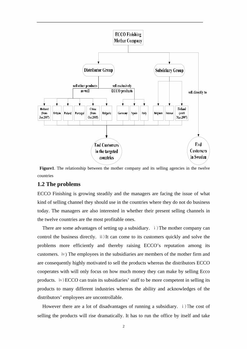
Figure1. The relationship between the mother company and its selling agencies in the twelve
countries
1.2 The problems ECCO Finishing is growing steadily and the managers are facing the issue of what
kind of selling channel they should use in the countries where they do not do business
today. The managers are also interested in whether their present selling channels in
the twelve countries are the most profitable ones.
There are some advantages of setting up a subsidiary. ⅰ)The mother company can
control the business directly. ⅱ)It can come to its customers quickly and solve the
problems more efficiently and thereby raising ECCO’s reputation among its
customers. ⅲ) The employees in the subsidiaries are members of the mother firm and
are consequently highly motivated to sell the products whereas the distributors ECCO
cooperates with will only focus on how much money they can make by selling Ecco
products. ⅳ)ECCO can train its subsidiaries’ staff to be more competent in selling its
products to many different industries whereas the ability and acknowledges of the
distributors’ employees are uncontrollable.
However there are a lot of disadvantages of running a subsidiary. ⅰ)The cost of
selling the products will rise dramatically. It has to run the office by itself and take
2

care of the expenses of running the office. ⅱ)There will be some monetary flow risk
as well as some operating risk. ⅲ)It needs time to build up its own reputation and get
enough loyal customers. ⅳ)It will be costly and difficult to work through its
subsidiaries to cover the whole market in the targeted country.
In order to obtain the target of maximum profit, the managers have to make the
correct decision on whether they should set up new subsidiary in the targeted
countries. This is exactly what this paper focuses on. The twelve countries will be
divided into two/three groups and endowed with two/three levels of treatments
according to different purposes of analysis. The definition of the levels of treatments
and explanations will be presented in detail in the following sections.
I take the “contribution margin” as the response variable and try to quantify all the
influencing factors by asking the main manager to give the scores of them. At the
same time I collect the data on the national basis for all the twelve countries, like
GNP, the average consumer prices and so on. I firstly apply a recently developed
method named propensity score to group the data and then using the refined dataset to
construct generalized linear mixed models (GLMMs). I also use the propensity score
to do the matching and analyse the differences of the outcome of the matched pairs
against the score.
The conclusion is that most of the twelve countries have been treated as they
should be treated, in a way which they can provide the maximum profit to the mother
company whereas in France and Germany exclusive distributors should be found for
them. Another conclusion is that theoretically speaking the higher the matching scores
the better the mother company should have a subsidiary in that country.
This paper is divided into four sections. In the next section the process of
smoothing the original financial data: the turnover and the contribution margin and
the data collected as the pre-treatment variables will be described. The third part is the
section describing the methods going to be used for this case. And in the very last
some strategic suggestions will be given based on the empirical findings.
2. Data In this section I firstly describe how I process the financial records into a smooth one
in order to facilitate the following analysis. Then I choose the response variable and
3

present a general description of it. Lastly I collect the influencing variables and
present explanations of them.
2.1 Processing of the financial records The original financial file contains two groups of data: turnover and contribution
margin from January 2004 to March 2008 on monthly basis. It is natural to have a
positive turnover and contribution margin on the book after one month hard working.
Whereas in the original data files sometimes the turnover is positive and the
contribution margin is negative followed with a negative margin ratio, and sometimes
the turnover is zero and a contribution margin is negative followed with a nonexistent
margin ratio.
After examination of another more detailed file which is on the daily basis, I figure
out the causes of the abnormal values. As the Table 1 show there are five kinds of
data records besides the daily transaction, which may have some impacts on the
turnover and contribution margin.
• KR = returned sales credit invoice (Both the turnover and contribution margin
are negative but they are not same.)
• KF = sales allowance credit invoice (Both the turnover and contribution
margin are negative and same.)
• FF = free text invoice (Used for example on advanced payments. Both the
turnover and contribution margin are positive.)
• Zero Sum invoices (Turnover equals to zero and contribution margin is
negative. This can be for example warranty, products fairs, tests etc)
• Discount selling (Turnover is positive whereas contribution margin is negative.
This can be for example get rid of old style products etc, and they sell products
at the price lower than the production cost)
These invoices are responsible for the negative month profit when the total regular
business’s profit in that month is less than the expenses. The invoices like KF, FF and
Zero Sum invoices should not be taken into account as that month’s expenses, instead
they should be considered as an expense throughout the whole year. So I decide to
add all the daily data back into monthly data and having the total of three types of
invoices spread out over the twelve months. I consider the KR as the regular
transaction with just the opposite direction. The “discount selling” has been left alone,
4
unless it is really big and liable for causing the negative profit. In that case I have to
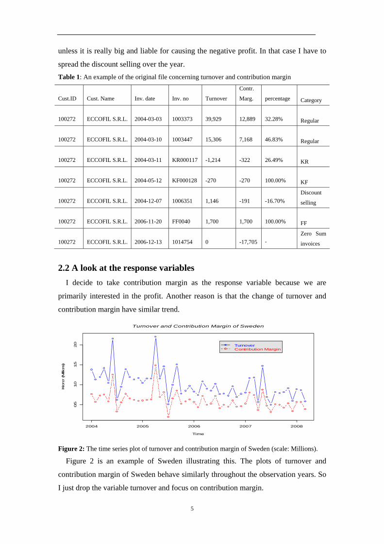
spread the discount selling over the year. Table 1: An example of the original file concerning turnover and contribution margin
Cust.ID Cust. Name Inv. date Inv. no Turnover
Contr.
Marg. percentage
Category
100272 ECCOFIL S.R.L. 2004-03-03 1003373 39,929 12,889 32.28%
Regular
100272 ECCOFIL S.R.L. 2004-03-10 1003447 15,306 7,168 46.83%
Regular
100272 ECCOFIL S.R.L. 2004-03-11 KR000117 -1,214 -322 26.49%
KR
100272 ECCOFIL S.R.L. 2004-05-12 KF000128 -270 -270 100.00%
KF
100272 ECCOFIL S.R.L. 2004-12-07 1006351 1,146 -191 -16.70% Discount
selling
100272 ECCOFIL S.R.L. 2006-11-20 FF0040 1,700 1,700 100.00%
FF
100272 ECCOFIL S.R.L. 2006-12-13 1014754 0 -17,705 - Zero Sum
invoices
2.2 A look at the response variables I decide to take contribution margin as the response variable because we are
primarily interested in the profit. Another reason is that the change of turnover and
contribution margin have similar trend.
Turnover and Contribution Margin of Sweden
Time
Krono
r (M
illions
)
2004 2005 2006 2007 2008
0.5
1.0
1.5
2.0 Turnover
Contribution Margin
Figure 2: The time series plot of turnover and contribution margin of Sweden (scale: Millions).
Figure 2 is an example of Sweden illustrating this. The plots of turnover and
contribution margin of Sweden behave similarly throughout the observation years. So
I just drop the variable turnover and focus on contribution margin.
5
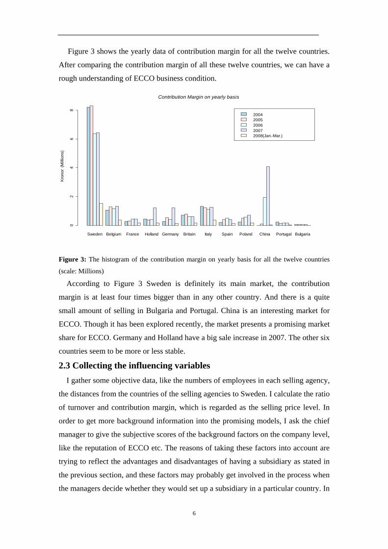
Figure 3 shows the yearly data of contribution margin for all the twelve countries.
After comparing the contribution margin of all these twelve countries, we can have a
rough understanding of ECCO business condition.
Sweden Belgium France Holland Germany Britain Italy Spain Poland China Portugal Bulgaria
20042005200620072008(Jan.-Mar.)
Kro
nor
(Mill
ions
)
02
46
8
Contribution Margin on yearly basis
Figure 3: The histogram of the contribution margin on yearly basis for all the twelve countries
(scale: Millions)
According to Figure 3 Sweden is definitely its main market, the contribution
margin is at least four times bigger than in any other country. And there is a quite
small amount of selling in Bulgaria and Portugal. China is an interesting market for
ECCO. Though it has been explored recently, the market presents a promising market
share for ECCO. Germany and Holland have a big sale increase in 2007. The other six
countries seem to be more or less stable.
2.3 Collecting the influencing variables I gather some objective data, like the numbers of employees in each selling agency,
the distances from the countries of the selling agencies to Sweden. I calculate the ratio
of turnover and contribution margin, which is regarded as the selling price level. In
order to get more background information into the promising models, I ask the chief
manager to give the subjective scores of the background factors on the company level,
like the reputation of ECCO etc. The reasons of taking these factors into account are
trying to reflect the advantages and disadvantages of having a subsidiary as stated in
the previous section, and these factors may probably get involved in the process when
the managers decide whether they would set up a subsidiary in a particular country. In
6
other words, these factors might largely affect the decision making process. By asking
the arbitrary scores, all the qualitative variables are quantified. At the same time some
variables of the twelve countries on the national level are found on the homepage of
the International Monetary Fund. They are annual data. All of these variables will be
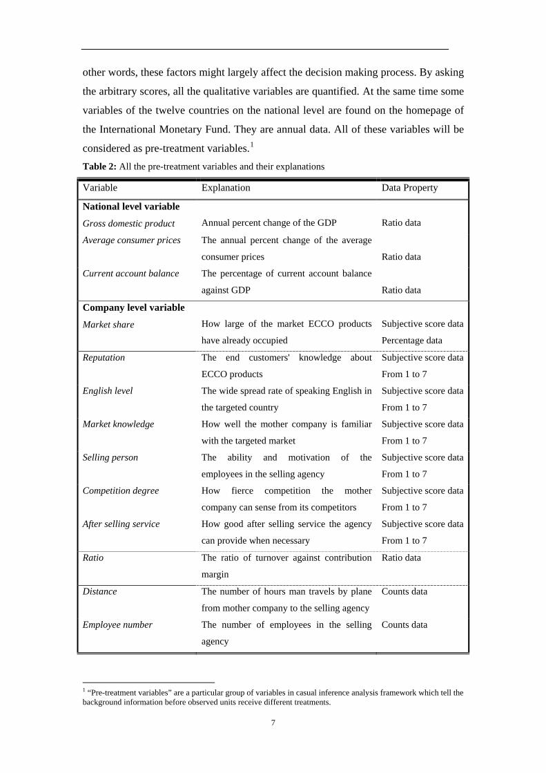
considered as pre-treatment variables.1
Table 2: All the pre-treatment variables and their explanations
Variable Explanation Data Property
National level variable
Gross domestic product
Annual percent change of the GDP
Ratio data
Average consumer prices The annual percent change of the average
consumer prices
Ratio data
Current account balance The percentage of current account balance
against GDP
Ratio data
Company level variable
Market share
How large of the market ECCO products
have already occupied
Subjective score data
Percentage data
Reputation The end customers' knowledge about
ECCO products
Subjective score data
From 1 to 7
English level The wide spread rate of speaking English in
the targeted country
Subjective score data
From 1 to 7
Market knowledge How well the mother company is familiar
with the targeted market
Subjective score data
From 1 to 7
Selling person The ability and motivation of the
employees in the selling agency
Subjective score data
From 1 to 7
Competition degree How fierce competition the mother
company can sense from its competitors
Subjective score data
From 1 to 7
After selling service How good after selling service the agency
can provide when necessary
Subjective score data
From 1 to 7
Ratio The ratio of turnover against contribution
margin
Ratio data
Distance The number of hours man travels by plane
from mother company to the selling agency
Counts data
Employee number The number of employees in the selling
agency
Counts data
1 “Pre-treatment variables” are a particular group of variables in casual inference analysis framework which tell the background information before observed units receive different treatments.
7

3. Method and model specification In this section I will first introduce the analysis framework of the casual inference
including its main concept “potential outcomes”, its potential problems “lack of
overlap”, “lack of balance” and the solving methods “propensity score”, “matching”.
Then I will apply this framework to my analysis and construct models for this
particular “selling channels” issue.
3.1 The overall analysis framework 3.1.1 The potential outcomes
This paper is interested in finding out which treatments: having their own
subsidiaries or working through distributors in some particular countries will bring
more profit to the mother company in Skara. This is an observational study for casual
effects. The first idea of the model to fit these data is to use generalized linear mixed
model (GLMM). But for the observational study we have to do the analysis with
caution when we are making causal inference. The problem is that in the
observational study there may be some kind of non-randomly intervention in the
treatment assignment process. In that case it is possible that for some units they will
be more likely to receive the treatment and for some other units they will be more
likely to receive the control treatment. Thus, if one just applies GLMM based on the
original dataset to fit these data the estimate will always be biased one. This is
because failing to get more concerned variables involved into the model. However, if
manages to do that, one probably can not get a significant estimate of the “treatment”
against the “outcome” which is the most important concern of this thesis.
Actually this is a typical potential outcome analysis framework which is introduced
by Rubin (1974). Let me take the two selling channels: subsidiary and distributor for a
two-level-treatment case as an example2. I state “having their own subsidiaries” as the
treated group with value “1” and the other “working through distributors” as the
control group with value “0”. The variable “contribution margin” is what the thesis is
concerned about and it is naturally taken as the outcome of the treatment. We are
eager to see how the treatment influences the outcome, or whether it makes some
differences for the outcome, which can be presented in the following way.
)0()1( iii YY −=τ (1)
Where means the th unit receives the b level treatment, b=1,0. )(bYi i 2 The three-level-treatment analysis can be extended in the similar way.
8

More specifically, the average treatment effect on all the units (ATE) is defined as
))0()1(()( iii YYEEATE −== τ (2)
And the average treatment effect on treated or control can be stated as ATT and
ATC respectively:
)1|)0(()1|)1(()1|( =−==== iiiiii TYETYETEATT τ (3)
)0|)0(()0|)1(()0|( =−==== iiiiii TYETYETEATC τ (4)
And this is the statistic for the estimates of (2)-(4):
∑=
−=−
N
i
ii
NYYYY
1
)0()1()0()1( jNi K2,1= (5)
Where )(bY means the average outcome which receives the b level treatment, b=1, 0.
is the number of the j units when j= “all”, “control” or “treated”. jN
The difficulty in this framework is that we will never know for sure what the
outcomes of control units are if they instead received the treatment and what the
outcomes of treated units are if they instead received the control treatment. In
equation (3) the estimate of expected non-treatment outcomes for the treated
is unknown and either is)1|)0(( =ii TYE )0|)1(( =ii TYE in equation (4). The key
issue is to find out a method to value these potential outcomes. It can be considered as
a missing value problem and that is why this framework is called potential outcomes
framework.
3.1.2 Matching method
Some talented people have figured out a feasible way to solve this systematic
problem by matching the similar units coming from different treatment groups. By
saying “similar” I mean the background information of each unit. In this paper it
should refer to the influencing variables I collect from ECCO Finishing as well as on
the Internet.
In order to do the matching and make reliable casual inference we have to make
an assumption in the beginning called ignorability.
Ignorability means when conditioned on confounding covariates in the analysis, X,
the potential outcomes are independent with the treatment variable. This concept is
always presented in the following formula:
.|)1(),0( XTYY ⊥ (6)
9

This assumption means the distribution of under )0(Y 1=T is same with the
distribution of under . And so is the case for . )0(Y 0=T )1(Y
This assumption gives us a theoretical support to find valid substitutes of
as )1|)0(( =ii TYE )0|)0(( =ii TYE and )0|)1(( =ii TYE as which is
an efficient approach to solve the systematic problem of the potential outcome
framework. Besides when the ignorability holds we are assured to model the data with
the pre-treatment variables and need not to bother ourselves about the treatment
assignment process. This is exactly what we can do in the complete randomized
experiments.
)1|)1(( =ii TYE
However in the observational experiment, it is always not as simple as that. “In
general, one can never prove that the treatment assignment process in an
observational study is ignorable—it is always possible that the choice of treatment
depends on relevant information that has not been recorded.”3 For the sake of
simplicity an assumption is made in this paper that this case satisfies the ignorability.
I ask the managers as many background variables as possible in order to assure most
of “the relevant information” has been recorded.
The assumption needs to be fulfilled to make the casual inference valid in using the
matching approach. Nonetheless, there are some other practical problems which
matching method is good at solving. The background variables are, more often than
not, more than one for each unit and thus they may have different characteristics
across the two groups. The typical phenomena for these differences are imbalance and
lack of complete overlap.
Imbalance means the distributions of the confounding covariates are not same
across groups. Lack of complete overlap refers to the condition when the ranges of the
data from different groups are not same. Figure 4 and 5 illustrate these concepts
fully.4
Figure 4: Two cases of imbalance of confounding covariates. The left case has different averages
and thus different distributions. The right one has same average but still different distributions.
3 Quoted sentence refer to the book Data Analysis Using Regression and Multilevel/ Hierarchical Model Page 184 4 Graphs refer to the book Data Analysis Using Regression and Multilevel/ Hierarchical Model Page 200-201
10

Figure 5: Three cases of lack of overlap. When in the partial overlap cases, one can only make
inference in the overlap ranges.
The presentation of these two situations will yield biased estimates of the causal
inference. Thus we have to appeal to matching or grouping in which process we get
similar units together in order to adjust for the pre-treatment differences across
groups.
In order to realize the matching or grouping, we have to appeal to another concept:
propensity score. Propensity score is the probability of being treated for each unit.
; )|()|1Pr( XTEXT == 1)|1Pr(0 <=< XT (7)
The calculation of the propensity score in practice can use the GLMM models
taking “treatment” as the response variable and the pre-treatment variables as the
covariates. And the link function can be the logit. In this paper, because of the three
level treatments, the multinomial model is used.
The propensity score sums up all the information of the pre-treatment variables to a
single number. We can match and group the observations according to this number
assuming that we will get matched pairs and groups having the similar backgrounds.
3.2 Empirical analysis 3.2.1 Three level treatment analysis
I decide to consider the twelve countries receiving treatments at three levels when I
explore the fact of the treatment effects, by dividing the distributor group into another
two subgroups. This is because it is natural to believe that different levels of
concentration in selling ECCO products may influence the profit the mother company
can earn. In addition from the variable “Employee number” I get to know that the
exclusive distributors are all small ones with no more than three employees whereas
the general distributors tend to be big ones. I define “T2” as the treatment level the subsidiary group receive which contains
countries: Sweden, Belgium, France and Holland (until 2007). “T1” is defined as
another treatment level group for the exclusive distributors which contains Italy,
Germany and Spain. And “C” is defined as the control group for the general
11
distributors which contains Holland (after 2007), Britain, China, Portugal, Bulgaria
and Poland.
First the multinomial model is used for calculating the propensity score which has
the treatments as the response variable and the pre-treatment variables as explanatory
variables. Thus each observation unit should have three probabilities of receiving
three levels treatments and their sum should be equal to one. I define the probability
of receiving treatment level “T2”, “T1” and “C” as “P2”, “P1 and “P0” respectively.
It is perfect if all the pre-treatment variables can be imposed into the model but due to
the high correlation among them I finally choose seven which are “English Level”,
“Distance”, “Employee number”, “log (Average Consumer Prices)”, “Ratio”, “After
Selling Service” and “Market Share”.
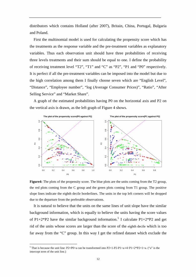
A graph of the estimated probabilities having P0 on the horizontal axis and P2 on
the vertical axis is drawn, as the left graph of Figure 4 shows.
0.0 0.2 0.4 0.6 0.8 1.0
0.0
0.2
0.4
0.6
0.8
1.0
The plot of the propensity score(P0 against P2)
P0
P2
0.0 0.2 0.4 0.6 0.8
0.0
0.2
0.4
0.6
0.8
1.0
The plot of the propensity score(P1 against P2)
P1
P2
Figure4: The plots of the propensity score. The blue plots are the units coming from the T2 group,
the red plots coming from the C group and the green plots coming from T1 group. The positive
slope lines indicate the eighth decile borderlines. The units in the top left corners will be dropped
due to the departure from the preferable observations.
It is natural to believe that the units on the same lines of unit slope have the similar
background information, which is equally to believe the units having the score values
of P1+2*P2 have the similar background information.5 I calculate P1+2*P2 and get
rid of the units whose scores are larger than the score of the eighth decile which is too
far away from the “C” group. In this way I get the refined dataset which exclude the
5 That is because the unit line: P2=P0+a can be transformed into P2=1-P2-P1+a P1+2*P2=1+a. (“a” is the intercept term of the unit line.)
⇒
12
units quite different from the common control observations and get its covariates
balanced to some degree. I call this refined dataset as “dataset 1”. Then I am assured
to fit the data with GLMM which I state as model 1.
The same process can be done with P1 replacing of P0 and I construct another
GLMM (model 2) with the refined dataset 2. In this dataset the score C+2*P2 should
be calculated, and the model is targeted for the T1 group.
The GLMMs have had the variable “treat” and all the seven pre-treatment variables
as the explanatory variables and log (contribution margin) as the response variable.
The random variable I choose is the country by each year, for example, Sweden2004,
Sweden2005 are two groups. The reason is that all the pre-treatment variables stay
constant through out the year for each country. Another reason is that during each
year the mother company and the selling agencies’ operating condition tend to stay
same, for example appointing another CEO or a change of strategy plan happens
probably in the end of each year. Thus grouping in this way can also include some
main factors which are difficult to detect or quantify but have potential crucial
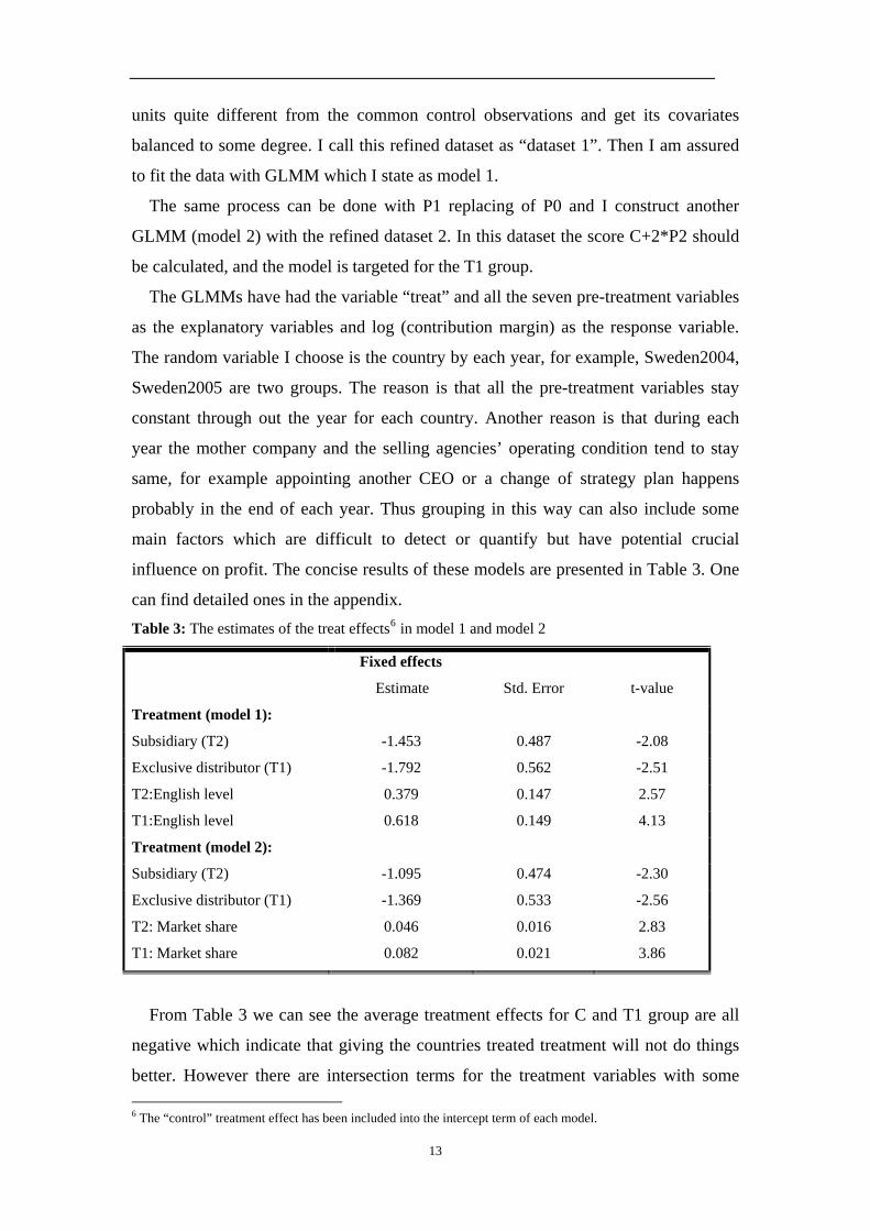
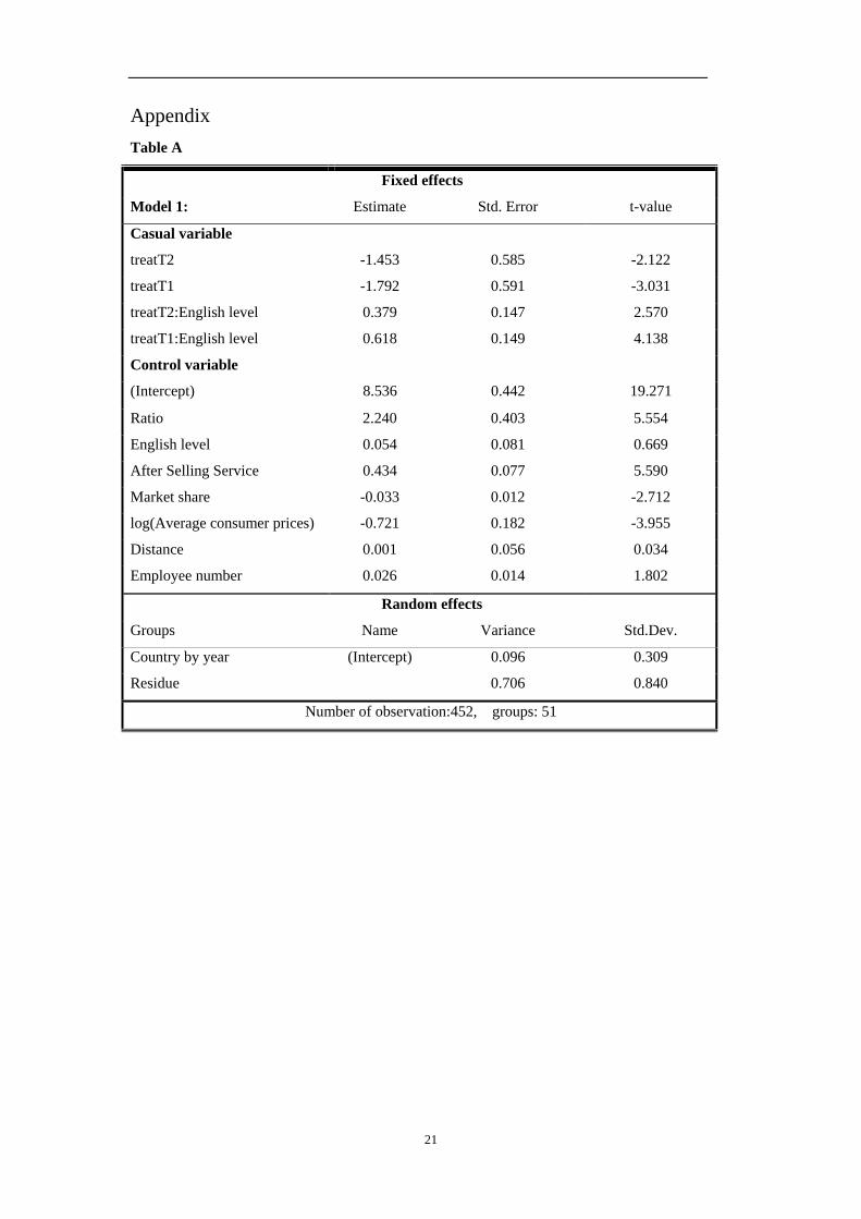
influence on profit. The concise results of these models are presented in Table 3. One
can find detailed ones in the appendix. Table 3: The estimates of the treat effects6 in model 1 and model 2
Fixed effects
Estimate Std. Error t-value
Treatment (model 1):
Subsidiary (T2) -1.453 0.487 -2.08
Exclusive distributor (T1) -1.792 0.562 -2.51
T2:English level 0.379 0.147 2.57
T1:English level 0.618 0.149 4.13
Treatment (model 2):
Subsidiary (T2) -1.095 0.474 -2.30
Exclusive distributor (T1) -1.369 0.533 -2.56
T2: Market share 0.046 0.016 2.83
T1: Market share 0.082 0.021 3.86
From Table 3 we can see the average treatment effects for C and T1 group are all
negative which indicate that giving the countries treated treatment will not do things
better. However there are intersection terms for the treatment variables with some 6 The “control” treatment effect has been included into the intercept term of each model.
13
other key variables, in this case English level and Market share, the estimates of
which are positive. Thus we can conclude that given high enough value of the key
pre-treatment variables the treat effect can turn into a positive one for some particular
countries. For example, the estimates of “subsidiary (T2)” and “T2: English level” are
-1.453 and 0.379. If the value of “English level” of a particular country is 4, the “T2”
treatment effect can be positive: -1.453+0.379*4=0.063>0. From which we can
conclude that the countries with the value of “English level” equal or bigger than 4
can do better given the “T2” treatment.
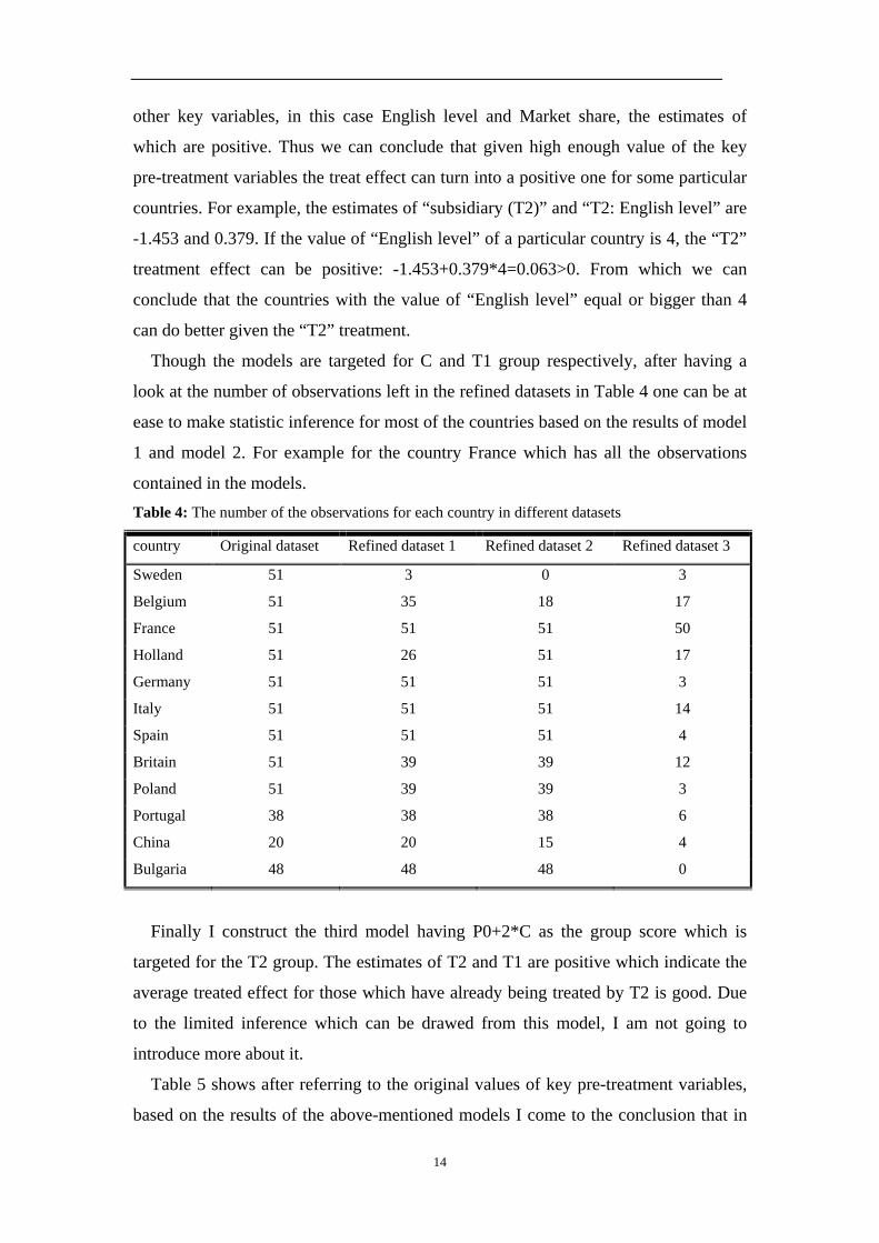
Though the models are targeted for C and T1 group respectively, after having a
look at the number of observations left in the refined datasets in Table 4 one can be at
ease to make statistic inference for most of the countries based on the results of model
1 and model 2. For example for the country France which has all the observations
contained in the models. Table 4: The number of the observations for each country in different datasets
country Original dataset Refined dataset 1 Refined dataset 2 Refined dataset 3
Sweden 51 3 0 3
Belgium 51 35 18 17
France 51 51 51 50
Holland 51 26 51 17
Germany 51 51 51 3
Italy 51 51 51 14
Spain 51 51 51 4
Britain 51 39 39 12
Poland 51 39 39 3
Portugal 38 38 38 6
China 20 20 15 4
Bulgaria 48 48 48 0
Finally I construct the third model having P0+2*C as the group score which is
targeted for the T2 group. The estimates of T2 and T1 are positive which indicate the
average treated effect for those which have already being treated by T2 is good. Due
to the limited inference which can be drawed from this model, I am not going to
introduce more about it.
Table 5 shows after referring to the original values of key pre-treatment variables,
based on the results of the above-mentioned models I come to the conclusion that in
14
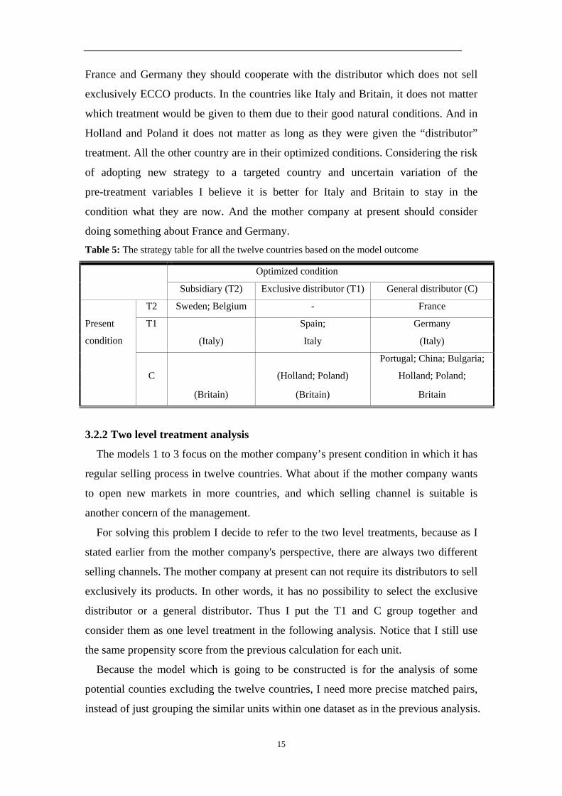
France and Germany they should cooperate with the distributor which does not sell
exclusively ECCO products. In the countries like Italy and Britain, it does not matter
which treatment would be given to them due to their good natural conditions. And in
Holland and Poland it does not matter as long as they were given the “distributor”
treatment. All the other country are in their optimized conditions. Considering the risk
of adopting new strategy to a targeted country and uncertain variation of the
pre-treatment variables I believe it is better for Italy and Britain to stay in the
condition what they are now. And the mother company at present should consider
doing something about France and Germany. Table 5: The strategy table for all the twelve countries based on the model outcome
Optimized condition
Subsidiary (T2) Exclusive distributor (T1) General distributor (C)
T2 Sweden; Belgium - France
T1 Spain; Germany Present
condition (Italy) Italy (Italy)
Portugal; China; Bulgaria;
C (Holland; Poland) Holland; Poland;
(Britain) (Britain) Britain
3.2.2 Two level treatment analysis
The models 1 to 3 focus on the mother company’s present condition in which it has
regular selling process in twelve countries. What about if the mother company wants
to open new markets in more countries, and which selling channel is suitable is
another concern of the management.
For solving this problem I decide to refer to the two level treatments, because as I
stated earlier from the mother company's perspective, there are always two different
selling channels. The mother company at present can not require its distributors to sell
exclusively its products. In other words, it has no possibility to select the exclusive
distributor or a general distributor. Thus I put the T1 and C group together and
consider them as one level treatment in the following analysis. Notice that I still use
the same propensity score from the previous calculation for each unit.
Because the model which is going to be constructed is for the analysis of some
potential counties excluding the twelve countries, I need more precise matched pairs,
instead of just grouping the similar units within one dataset as in the previous analysis.
15
In other words, for the sake of universality I need matched pairs having the similar
background in a much more refined dataset. I first get rid of extreme observations by
drawing an inscribed circle of the triangle in the left score plot of figure 4. The units
within the circle have been preserved. 272 units out of 565 units have been dropped in
this stage. Then I use the score T1+2*T2 as the matching score and do the matching
with replacement. In this matching process the two observations coming from
different levels of treatments will be put into a match according to the value of
T1+2*T2, the R program will find the nearest unit for each treated unit. “Matching
with replacement” means same control units can be matched to different treated units
more than once. I set the caliper equalled to 0.25 which means that if the difference of
the scores of the treated unit with its nearest matched control unit is more than 0.25,
the treated unit will be dropped. Now the dataset has only 133 observations with 82
matched pairs.
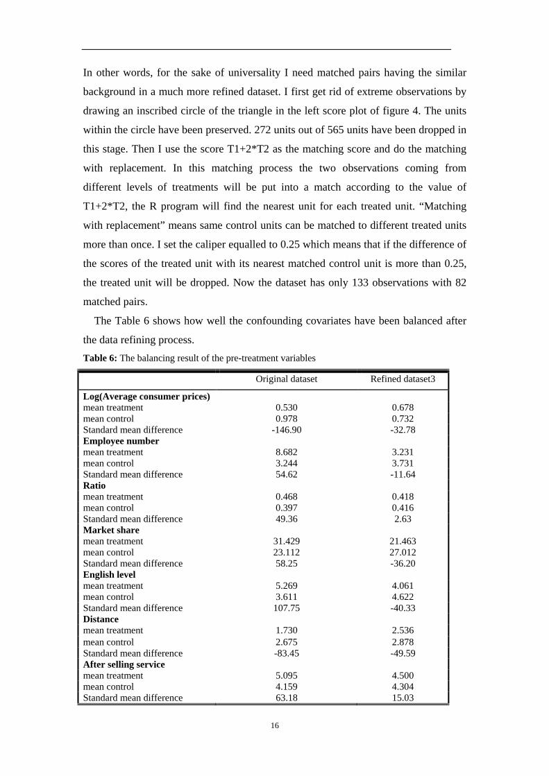
The Table 6 shows how well the confounding covariates have been balanced after
the data refining process. Table 6: The balancing result of the pre-treatment variables
Original dataset Refined dataset3
Log(Average consumer prices) mean treatment 0.530 0.678 mean control 0.978 0.732 Standard mean difference -146.90 -32.78 Employee number mean treatment 8.682 3.231 mean control 3.244 3.731 Standard mean difference 54.62 -11.64 Ratio mean treatment 0.468 0.418 mean control 0.397 0.416 Standard mean difference 49.36 2.63 Market share mean treatment 31.429 21.463 mean control 23.112 27.012 Standard mean difference 58.25 -36.20 English level mean treatment 5.269 4.061 mean control 3.611 4.622 Standard mean difference 107.75 -40.33 Distance mean treatment 1.730 2.536 mean control 2.675 2.878 Standard mean difference -83.45 -49.59 After selling service mean treatment 5.095 4.500 mean control 4.159 4.304 Standard mean difference 63.18 15.03
16
As one can see the standard mean differences have been reduced greatly and the
means of the variables coming from treatment and control groups tend to come closer
to each other.
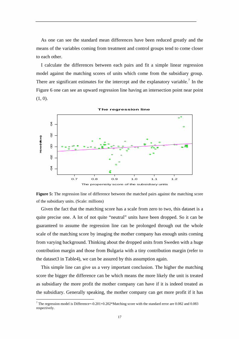
I calculate the differences between each pairs and fit a simple linear regression
model against the matching scores of units which come from the subsidiary group.
There are significant estimates for the intercept and the explanatory variable.7 In the
Figure 6 one can see an upward regression line having an intersection point near point
(1, 0).
0.7 0.8 0.9 1.0 1.1 1.2
-0.4
-0.2
0.0
0.2
0.4
The regression line
The propensity score of the subsidiary units
Krono
r (Millions)
Figure 5: The regression line of difference between the matched pairs against the matching score
of the subsidiary units. (Scale: millions)
Given the fact that the matching score has a scale from zero to two, this dataset is a
quite precise one. A lot of not quite “neutral” units have been dropped. So it can be
guaranteed to assume the regression line can be prolonged through out the whole
scale of the matching score by imaging the mother company has enough units coming
from varying background. Thinking about the dropped units from Sweden with a huge
contribution margin and those from Bulgaria with a tiny contribution margin (refer to
the dataset3 in Table4), we can be assured by this assumption again.
This simple line can give us a very important conclusion. The higher the matching
score the bigger the difference can be which means the more likely the unit is treated
as subsidiary the more profit the mother company can have if it is indeed treated as
the subsidiary. Generally speaking, the mother company can get more profit if it has 7 The regression model is Difference=-0.201+0.202*Matching score with the standard error are 0.082 and 0.083 respectively.
17

more subsidiaries given a high matching score and has more distributors given a low
matching score. From another perspective this model actually is in line with the
results I get from GLMMs that most of the countries have been treated in a way which
they should be treated.
4. Discussion and further improvement Because of the characteristics of the data this research rely more on the model
specification rather than the data itself. That is why using different models one can
come to different conclusions. Comfortingly they all support the common general
conclusions which are in the following. Firstly, most countries are being treated in a
way which they should be treated. Secondly, France and Germany should switch to
general distributors which sell many other products as well. In practice it may be
difficult for the mother company to find such distributors in these two countries.
However this conclusion at least reminds the management that having subsidiaries in
these two countries is not a good idea. Thirdly, the higher the matching score
T1+2*T2 the better if the countries were treated as subsidiaries which provide the
management a auxiliary tool for their decision for some other new targeted markets in
the future. But because the present countries are all European countries except China
this conclusion should be safely used in the similar countries in the Europe or big
country in Asia like India.
Of course in this paper there are still some problems which are difficult to solve. In
this case we have access to the book data. However, the problems like the strategic
decision sometimes difficult to solve if just using the book data. The unusual events,
through they are not common to occur, as long as they occurred they would impose
great influence greatly on the result, for example in Germany there is only one person
being responsible of selling ECCO products and when he can not work due to some
personal reasons, the profit earned in Germany would be influenced. Another example
is there is a big customer in Sweden who will have the new production line every four
years and for ECCO it can make an extra profit equals to four million. Such random
factors are difficult to comprise in a model.
For further improvement, we should improve the quality of the background
variables by collecting more reliable data instead of just the subjective score and
come to detail about the distributors’ operating conditions. It maybe difficult to get
18

precise data from the distributors due to their confidential concern, but we can record
daily tiny activities like the frequency the selling persons in the mother company
come to visit the distributors and how many times there have the products fairs in the
countries and arrange the data on fixed time intervals. Another improvement in the
model may be skipping the assumption of ignorability and considering other method
like instrument variable to solve this “selling channels” problem.
19

Reference [1] Andrew Gelman, Jennifer Hill. (2007). Data Analysis Using Regression and Multievel/ Hierarchical Models. Cambridge University Press. 3rd printing. [2] Wang, I.J.W., Alam, M. (2007). When are non-experimental estimates close to experimental estimates? Evidence from a study of summer job effects in Sweden. Presented paper at the EALE Conference 2007, URL: http://www.eale.nl/conference2007/programme/Papers%20Friday%2014.00%20-%2016.00/add45429.pdf[3] Wang-Sheng Lee. (2006). Propensity Score Matching and Variations on the Balancing Test. https://editorialexpress.com/cgi-bin/conference/download.cgi?db_name=esam06&paper_id=217 [4] Rajeev H. Dehejia, Sadek Wahba. (2002). Propensity score-matching methods for nonexperimental causal studies. The Review of Economics and Statistics. 84(1): 151–161. [5] P. McCullagh, John A. Nelder. (1989). Generalized Linear Models, Second Edition, Chapman & Hall/CRC. [6] Ulf Olsson. (2002). Generalized Linear Models: An Applied Approach. Student literature AB. [7] Paul R. Rosenbaum, Donald B. Rubin. (1983). The Central Role of the Propensity Score in Observational Studies for Causal Effects. Biometrika. 70,1,pp.41-55. [8] Donald R. Rubin. (1974). Estimating casual effects of treatments in randomized and nonrandomized studies. Journal of Education Psychology. 66, 688-701. [9] Donald R. Rubin. (2004). Causal Inference Using Potential Outcomes: Design, Modeling, Decisions. Journal of the American Statistical Association. 100,3, pp.322-331.
20
Appendix Table A
Fixed effects
Model 1: Estimate Std. Error t-value
Casual variable
treatT2 -1.453 0.585 -2.122
treatT1 -1.792 0.591 -3.031
treatT2:English level 0.379 0.147 2.570
treatT1:English level 0.618 0.149 4.138
Control variable
(Intercept) 8.536 0.442 19.271
Ratio 2.240 0.403 5.554
English level 0.054 0.081 0.669
After Selling Service 0.434 0.077 5.590
Market share -0.033 0.012 -2.712
log(Average consumer prices) -0.721 0.182 -3.955
Distance 0.001 0.056 0.034
Employee number 0.026 0.014 1.802
Random effects
Groups Name Variance Std.Dev.
Country by year (Intercept) 0.096 0.309
Residue 0.706 0.840
Number of observation:452, groups: 51
21
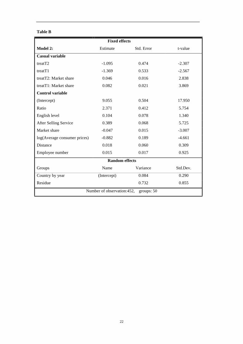
Table B
Fixed effects
Model 2: Estimate Std. Error t-value
Casual variable
treatT2 -1.095 0.474 -2.307
treatT1 -1.369 0.533 -2.567
treatT2: Market share 0.046 0.016 2.838
treatT1: Market share 0.082 0.021 3.869
Control variable
(Intercept) 9.055 0.504 17.950
Ratio 2.371 0.412 5.754
English level 0.104 0.078 1.340
After Selling Service 0.389 0.068 5.725
Market share -0.047 0.015 -3.007
log(Average consumer prices) -0.882 0.189 -4.661
Distance 0.018 0.060 0.309
Employee number 0.015 0.017 0.925
Random effects
Groups Name Variance Std.Dev.
Country by year (Intercept) 0.084 0.290
Residue 0.732 0.855
Number of observation:452, groups: 50
22