An Introduction to Stochastic Multi-armed Bandits
70
1/21 An Introduction to Stochastic Multi-armed Bandits Shivaram Kalyanakrishnan [email protected] Department of Computer Science and Automation Indian Institute of Science August 2014 Shivaram Kalyanakrishnan (2014) Multi-armed Bandits 1 / 21
Transcript of An Introduction to Stochastic Multi-armed Bandits

1/21
An Introduction to Stochastic Multi-armed Bandits
Shivaram [email protected]
Department of Computer Science and AutomationIndian Institute of Science
August 2014
Shivaram Kalyanakrishnan (2014) Multi-armed Bandits 1 / 21

2/21
Today’s Talk
� What we will cover
Shivaram Kalyanakrishnan (2014) Multi-armed Bandits 2 / 21

2/21
Today’s Talk
� What we will cover
- Stochasticbandits
Shivaram Kalyanakrishnan (2014) Multi-armed Bandits 2 / 21

2/21
Today’s Talk
� What we will cover
- Stochasticbandits
� What we will not cover
Shivaram Kalyanakrishnan (2014) Multi-armed Bandits 2 / 21

2/21
Today’s Talk
� What we will cover
- Stochasticbandits
� What we will not cover
- Adversarialbandits
Shivaram Kalyanakrishnan (2014) Multi-armed Bandits 2 / 21

2/21
Today’s Talk
� What we will cover
- Stochasticbandits
� What we will not cover
- Adversarialbandits- Duelingbandits
Shivaram Kalyanakrishnan (2014) Multi-armed Bandits 2 / 21

2/21
Today’s Talk
� What we will cover
- Stochasticbandits
� What we will not cover
- Adversarialbandits- Duelingbandits- Contextualbandits
Shivaram Kalyanakrishnan (2014) Multi-armed Bandits 2 / 21

2/21
Today’s Talk
� What we will cover
- Stochasticbandits
� What we will not cover
- Adversarialbandits- Duelingbandits- Contextualbandits- Mortal bandits
Shivaram Kalyanakrishnan (2014) Multi-armed Bandits 2 / 21

2/21
Today’s Talk
� What we will cover
- Stochasticbandits
� What we will not cover
- Adversarialbandits- Duelingbandits- Contextualbandits- Mortal bandits- Sleepingbandits
Shivaram Kalyanakrishnan (2014) Multi-armed Bandits 2 / 21

2/21
Today’s Talk
� What we will cover
- Stochasticbandits
� What we will not cover
- Adversarialbandits- Duelingbandits- Contextualbandits- Mortal bandits- Sleepingbandits- Realbandits
Shivaram Kalyanakrishnan (2014) Multi-armed Bandits 2 / 21

3/21
A Game
Coin 1 Coin 2 Coin 3
P{heads} = p1 P{heads} = p2 P{heads} = p3
� p1, p2, andp3 areunknown.
� You are given a total of 20 tosses.
� Maximise the total number of heads!
Shivaram Kalyanakrishnan (2014) Multi-armed Bandits 3 / 21

4/21
To Explore or to Exploit?
� On-line advertising: Template optimisation
CARS
CARS
Cars?
Shivaram Kalyanakrishnan (2014) Multi-armed Bandits 4 / 21

4/21
To Explore or to Exploit?
� On-line advertising: Template optimisation
CARS
CARS
Cars?
� Clinical trials (Robbins, 1952)
Shivaram Kalyanakrishnan (2014) Multi-armed Bandits 4 / 21

4/21
To Explore or to Exploit?
� On-line advertising: Template optimisation
CARS
CARS
Cars?
� Clinical trials (Robbins, 1952)
� Packet routing in communication networks (Altman, 2002)
Shivaram Kalyanakrishnan (2014) Multi-armed Bandits 4 / 21

4/21
To Explore or to Exploit?
� On-line advertising: Template optimisation
CARS
CARS
Cars?
� Clinical trials (Robbins, 1952)
� Packet routing in communication networks (Altman, 2002)
� Game playing and reinforcement learning (Kocsis and Szepesvári, 2006)
Shivaram Kalyanakrishnan (2014) Multi-armed Bandits 4 / 21
5/21
Overview
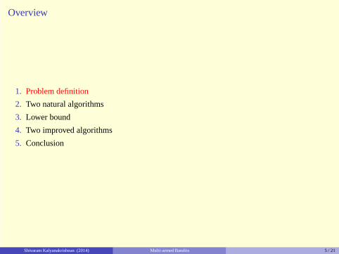
1. Problem definition
2. Two natural algorithms
3. Lower bound
4. Two improved algorithms
5. Conclusion
Shivaram Kalyanakrishnan (2014) Multi-armed Bandits 5 / 21

6/21
Stochastic Multi-armed Bandits
R
1
0
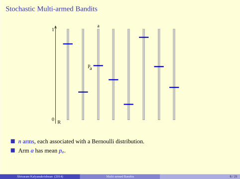
� n arms, each associated with a Bernoulli distribution.
Shivaram Kalyanakrishnan (2014) Multi-armed Bandits 6 / 21
6/21
Stochastic Multi-armed Bandits
pa
a
R
1
0
� n arms, each associated with a Bernoulli distribution.
� Arm a has meanpa.
Shivaram Kalyanakrishnan (2014) Multi-armed Bandits 6 / 21
6/21
Stochastic Multi-armed Bandits
pa
a
R
1
0
p*
� n arms, each associated with a Bernoulli distribution.
� Arm a has meanpa.
� Highest mean isp∗.
Shivaram Kalyanakrishnan (2014) Multi-armed Bandits 6 / 21

7/21
One-armed Bandits
Shivaram Kalyanakrishnan (2014) Multi-armed Bandits 7 / 21

8/21
Regret Minimisation
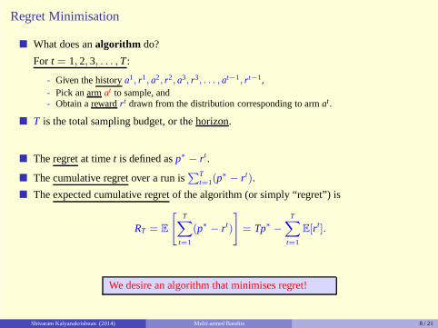
� What does analgorithm do?
Shivaram Kalyanakrishnan (2014) Multi-armed Bandits 8 / 21

8/21
Regret Minimisation
� What does analgorithm do?
For t = 1, 2, 3, . . . , T :
- Given the historya1, r1, a2, r2, a3, r3, . . . , at−1, rt−1,- Pick an armat to sample, and- Obtain a rewardrt drawn from the distribution corresponding to armat.
� T is the total sampling budget, or the horizon.
� The regretat timet is defined asp∗ − rt.
� The cumulative regretover a run isPT
t=1(p∗ − rt).
� The expected cumulative regretof the algorithm (or simply “regret”) is
RT = E
"
TX
t=1
(p∗ − rt)
#
= Tp∗ −T
X
t=1
E[rt].
Shivaram Kalyanakrishnan (2014) Multi-armed Bandits 8 / 21
8/21
Regret Minimisation
� What does analgorithm do?
For t = 1, 2, 3, . . . , T :
- Given the historya1, r1, a2, r2, a3, r3, . . . , at−1, rt−1,- Pick an armat to sample, and- Obtain a rewardrt drawn from the distribution corresponding to armat.
� T is the total sampling budget, or the horizon.
� The regretat timet is defined asp∗ − rt.
� The cumulative regretover a run isPT
t=1(p∗ − rt).
� The expected cumulative regretof the algorithm (or simply “regret”) is
RT = E
"
TX
t=1
(p∗ − rt)
#
= Tp∗ −T
X
t=1
E[rt].
We desire an algorithm that minimises regret!
Shivaram Kalyanakrishnan (2014) Multi-armed Bandits 8 / 21

9/21
Overview
1. Problem definition
2. Two natural algorithms
3. Lower bound
4. Two improved algorithms
5. Conclusion
Shivaram Kalyanakrishnan (2014) Multi-armed Bandits 9 / 21
10/21
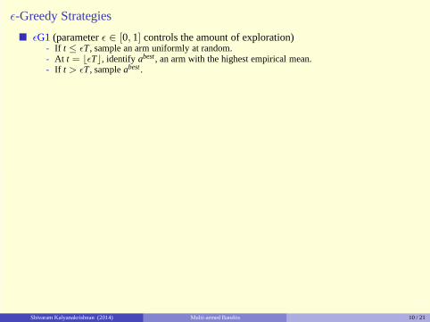
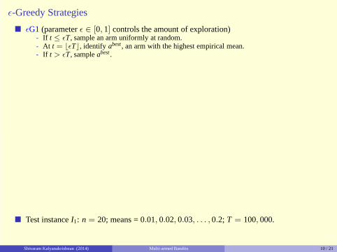
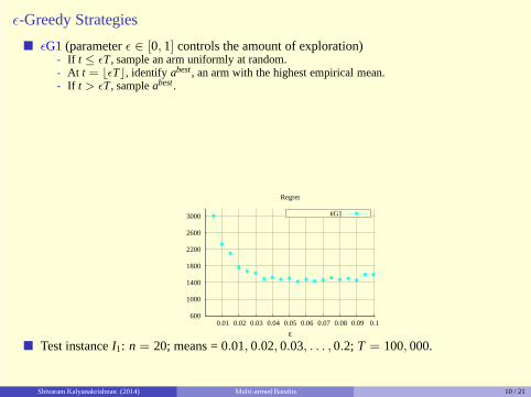
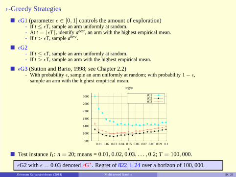
ǫ-Greedy Strategies
� ǫG1(parameterǫ ∈ [0, 1] controls the amount of exploration)- If t ≤ ǫT, sample an arm uniformly at random.- At t = ⌊ǫT⌋, identify abest , an arm with the highest empirical mean.- If t > ǫT, sampleabest .
Shivaram Kalyanakrishnan (2014) Multi-armed Bandits 10 / 21
10/21
ǫ-Greedy Strategies
� ǫG1(parameterǫ ∈ [0, 1] controls the amount of exploration)- If t ≤ ǫT, sample an arm uniformly at random.- At t = ⌊ǫT⌋, identify abest , an arm with the highest empirical mean.- If t > ǫT, sampleabest .
� Test instanceI1: n = 20; means = 0.01, 0.02, 0.03, . . . , 0.2; T = 100, 000.
Shivaram Kalyanakrishnan (2014) Multi-armed Bandits 10 / 21
10/21
ǫ-Greedy Strategies
� ǫG1(parameterǫ ∈ [0, 1] controls the amount of exploration)- If t ≤ ǫT, sample an arm uniformly at random.- At t = ⌊ǫT⌋, identify abest , an arm with the highest empirical mean.- If t > ǫT, sampleabest .
3000
2600
2200
1800
1400
1000
600 0.1 0.09 0.08 0.07 0.06 0.05 0.04 0.03 0.02 0.01
ε
Regret
εG1
� Test instanceI1: n = 20; means = 0.01, 0.02, 0.03, . . . , 0.2; T = 100, 000.
Shivaram Kalyanakrishnan (2014) Multi-armed Bandits 10 / 21

10/21
ǫ-Greedy Strategies
� ǫG1(parameterǫ ∈ [0, 1] controls the amount of exploration)- If t ≤ ǫT, sample an arm uniformly at random.- At t = ⌊ǫT⌋, identify abest , an arm with the highest empirical mean.- If t > ǫT, sampleabest .
� ǫG2- If t ≤ ǫT, sample an arm uniformly at random.- If t > ǫT, sample an arm with the highest empirical mean.
3000
2600
2200
1800
1400
1000
600 0.1 0.09 0.08 0.07 0.06 0.05 0.04 0.03 0.02 0.01
ε
Regret
εG1εG2
� Test instanceI1: n = 20; means = 0.01, 0.02, 0.03, . . . , 0.2; T = 100, 000.
Shivaram Kalyanakrishnan (2014) Multi-armed Bandits 10 / 21

10/21
ǫ-Greedy Strategies
� ǫG1(parameterǫ ∈ [0, 1] controls the amount of exploration)- If t ≤ ǫT, sample an arm uniformly at random.- At t = ⌊ǫT⌋, identify abest , an arm with the highest empirical mean.- If t > ǫT, sampleabest .
� ǫG2- If t ≤ ǫT, sample an arm uniformly at random.- If t > ǫT, sample an arm with the highest empirical mean.
� ǫG3(Sutton and Barto, 1998; see Chapter 2.2)- With probabilityǫ, sample an arm uniformly at random; with probability 1− ǫ,
sample an arm with the highest empirical mean.
3000
2600
2200
1800
1400
1000
600 0.1 0.09 0.08 0.07 0.06 0.05 0.04 0.03 0.02 0.01
ε
Regret
εG1εG2εG3
� Test instanceI1: n = 20; means = 0.01, 0.02, 0.03, . . . , 0.2; T = 100, 000.
Shivaram Kalyanakrishnan (2014) Multi-armed Bandits 10 / 21
10/21
ǫ-Greedy Strategies
� ǫG1(parameterǫ ∈ [0, 1] controls the amount of exploration)- If t ≤ ǫT, sample an arm uniformly at random.- At t = ⌊ǫT⌋, identify abest , an arm with the highest empirical mean.- If t > ǫT, sampleabest .
� ǫG2- If t ≤ ǫT, sample an arm uniformly at random.- If t > ǫT, sample an arm with the highest empirical mean.
� ǫG3(Sutton and Barto, 1998; see Chapter 2.2)- With probabilityǫ, sample an arm uniformly at random; with probability 1− ǫ,
sample an arm with the highest empirical mean.
3000
2600
2200
1800
1400
1000
600 0.1 0.09 0.08 0.07 0.06 0.05 0.04 0.03 0.02 0.01
ε
Regret
εG1εG2εG3
� Test instanceI1: n = 20; means = 0.01, 0.02, 0.03, . . . , 0.2; T = 100, 000.
ǫG2 with ǫ = 0.03 denotedǫG∗. Regret of822± 24 over a horizon of 100, 000.
Shivaram Kalyanakrishnan (2014) Multi-armed Bandits 10 / 21

11/21
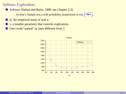
Softmax Exploration� Softmax(Sutton and Barto, 1998; see Chapter 2.3)
- At time t, Sample arma with probability proportional toexp“
αp̂taTt
”
.
� p̂ta the empirical mean of arma.
� α a tunable parameter that controls exploration.
� One could “anneal” at rates different from1t .
Shivaram Kalyanakrishnan (2014) Multi-armed Bandits 11 / 21
11/21
Softmax Exploration� Softmax(Sutton and Barto, 1998; see Chapter 2.3)
- At time t, Sample arma with probability proportional toexp“
αp̂taTt
”
.
� p̂ta the empirical mean of arma.
� α a tunable parameter that controls exploration.
� One could “anneal” at rates different from1t .
600
800
1000
1200
1400
1600
1800
2000
2200
20 40 60 80 100 120 140 160 180 200
α
Regret
Softmax
Shivaram Kalyanakrishnan (2014) Multi-armed Bandits 11 / 21

11/21
Softmax Exploration� Softmax(Sutton and Barto, 1998; see Chapter 2.3)
- At time t, Sample arma with probability proportional toexp“
αp̂taTt
”
.
� p̂ta the empirical mean of arma.
� α a tunable parameter that controls exploration.
� One could “anneal” at rates different from1t .
600
800
1000
1200
1400
1600
1800
2000
2200
20 40 60 80 100 120 140 160 180 200
α
Regret
Softmax
Softmax withα = 100 denotedSoftmax∗. Regret of720± 13 onI1 over a horizon ofT = 100, 000.
Shivaram Kalyanakrishnan (2014) Multi-armed Bandits 11 / 21
12/21
Overview
1. Problem definition
2. Two natural algorithms
3. Lower bound
4. Two improved algorithms
5. Conclusion
Shivaram Kalyanakrishnan (2014) Multi-armed Bandits 12 / 21

13/21
A Lower Bound on Regret
Paraphrasing Lai and Robbins (1985; see Theorem 2).
LetA be an algorithm such that for everybandit instanceI and for everya > 0, asT → ∞:
RT(A, I) = o(Ta).
Shivaram Kalyanakrishnan (2014) Multi-armed Bandits 13 / 21

13/21
A Lower Bound on Regret
Paraphrasing Lai and Robbins (1985; see Theorem 2).
LetA be an algorithm such that for everybandit instanceI and for everya > 0, asT → ∞:
RT(A, I) = o(Ta).
Then, for everybandit instanceI, asT → ∞:
RT(A, I) ≥
0
@
X
a:pa(I) 6=p∗(I)
p∗(I) − pa(I)KL(pa(I), p∗(I))
1
A log(T).
Shivaram Kalyanakrishnan (2014) Multi-armed Bandits 13 / 21

14/21
Overview
1. Problem definition
2. Two natural algorithms
3. Lower bound
4. Two improved algorithms
5. Conclusion
Shivaram Kalyanakrishnan (2014) Multi-armed Bandits 14 / 21

15/21
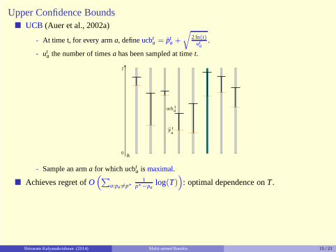
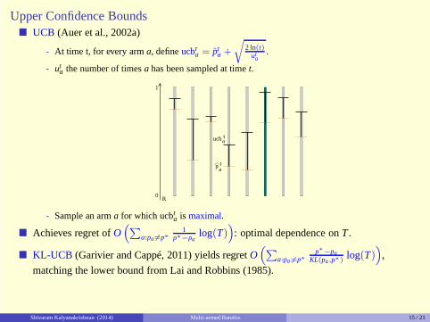
Upper Confidence Bounds� UCB (Auer et al., 2002a)
- At time t, for every arma, defineucbta = p̂t
a +
r
2 ln(t)ut
a.
- uta the number of timesa has been sampled at timet.
R
1
0
pat
ucbat
Shivaram Kalyanakrishnan (2014) Multi-armed Bandits 15 / 21

15/21
Upper Confidence Bounds� UCB (Auer et al., 2002a)
- At time t, for every arma, defineucbta = p̂t
a +
r
2 ln(t)ut
a.
- uta the number of timesa has been sampled at timet.
R
1
0
pat
ucbat
- Sample an arma for which ucbta is maximal.
Shivaram Kalyanakrishnan (2014) Multi-armed Bandits 15 / 21

15/21
Upper Confidence Bounds� UCB (Auer et al., 2002a)
- At time t, for every arma, defineucbta = p̂t
a +
r
2 ln(t)ut
a.
- uta the number of timesa has been sampled at timet.
R
1
0
pat
ucbat
- Sample an arma for which ucbta is maximal.
Shivaram Kalyanakrishnan (2014) Multi-armed Bandits 15 / 21
15/21
Upper Confidence Bounds� UCB (Auer et al., 2002a)
- At time t, for every arma, defineucbta = p̂t
a +
r
2 ln(t)ut
a.
- uta the number of timesa has been sampled at timet.
R
1
0
pat
ucbat
- Sample an arma for which ucbta is maximal.
� Achieves regret ofO“
P
a:pa 6=p∗1
p∗−palog(T)
”
: optimal dependence onT .
� KL-UCB (Garivier and Cappé, 2011) yields regretO“
P
a:pa 6=p∗p∗−pa
KL(pa,p∗)log(T)
”
,
matching the lower bound from Lai and Robbins (1985).
Shivaram Kalyanakrishnan (2014) Multi-armed Bandits 15 / 21

15/21
Upper Confidence Bounds� UCB (Auer et al., 2002a)
- At time t, for every arma, defineucbta = p̂t
a +
r
2 ln(t)ut
a.
- uta the number of timesa has been sampled at timet.
R
1
0
pat
ucbat
- Sample an arma for which ucbta is maximal.
� Achieves regret ofO“
P
a:pa 6=p∗1
p∗−palog(T)
”
: optimal dependence onT .
� KL-UCB (Garivier and Cappé, 2011) yields regretO“
P
a:pa 6=p∗p∗−pa
KL(pa,p∗)log(T)
”
,
matching the lower bound from Lai and Robbins (1985).
Regret on instanceI1 (with T = 100, 000)–UCB:1168± 16; KL-UCB: 738± 18.
Shivaram Kalyanakrishnan (2014) Multi-armed Bandits 15 / 21

16/21
Thompson Sampling� Thompson(Thompson, 1933)
- At time t, let arma havesta successes (ones) andf t
a failures (zeroes).
Shivaram Kalyanakrishnan (2014) Multi-armed Bandits 16 / 21

16/21
Thompson Sampling� Thompson(Thompson, 1933)
- At time t, let arma havesta successes (ones) andf t
a failures (zeroes).
- Beta(sta + 1, f t
a + 1) represents a “belief” about the true mean of arma.
- Mean =sta+1
sta+f t
a+2 ; variance =(st
a+1)(f ta+1)
(sta+f t
a+2)2(sta+f t
a+3).
R
1
0
- Computational step: For every arma, draw a samplexta ∼ Beta(st
a + 1, f ta + 1).
- Sampling step:Sample an arma for which xta is maximal.
� Achievesoptimal regret(Kaufmann et al., 2012); isexcellent in practice(Chapelle and Li, 2011).
On instanceI1 (with T = 100, 000), regret is463± 18.
Shivaram Kalyanakrishnan (2014) Multi-armed Bandits 16 / 21

17/21
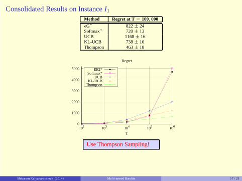
Consolidated Results on InstanceI1
Method Regret at T = 100, 000
ǫG∗ 822± 24Softmax∗ 720± 13UCB 1168± 16KL-UCB 738± 16Thompson 463± 18
Shivaram Kalyanakrishnan (2014) Multi-armed Bandits 17 / 21

17/21
Consolidated Results on InstanceI1
Method Regret at T = 100, 000
ǫG∗ 822± 24Softmax∗ 720± 13UCB 1168± 16KL-UCB 738± 16Thompson 463± 18
0
1000
2000
3000
4000
5000
106105104103102
T
Regret
EE2*Softmax*
UCBKL-UCB
Thompson
Shivaram Kalyanakrishnan (2014) Multi-armed Bandits 17 / 21
17/21
Consolidated Results on InstanceI1
Method Regret at T = 100, 000
ǫG∗ 822± 24Softmax∗ 720± 13UCB 1168± 16KL-UCB 738± 16Thompson 463± 18
0
1000
2000
3000
4000
5000
106105104103102
T
Regret
EE2*Softmax*
UCBKL-UCB
Thompson
Use Thompson Sampling!
Shivaram Kalyanakrishnan (2014) Multi-armed Bandits 17 / 21

17/21
Consolidated Results on InstanceI1
Method Regret at T = 100, 000
ǫG∗ 822± 24Softmax∗ 720± 13UCB 1168± 16KL-UCB 738± 16Thompson 463± 18
0
1000
2000
3000
4000
5000
106105104103102
T
Regret
EE2*Softmax*
UCBKL-UCB
Thompson
Use Thompson Sampling!
Principle: “Optimism in the face of uncertainty.”
Shivaram Kalyanakrishnan (2014) Multi-armed Bandits 17 / 21

18/21
Overview
1. Problem definition
2. Two natural algorithms
3. Lower bound
4. Two improved algorithms
5. Conclusion
Shivaram Kalyanakrishnan (2014) Multi-armed Bandits 18 / 21

19/21
Discussion
� Challenges and extensions
Shivaram Kalyanakrishnan (2014) Multi-armed Bandits 19 / 21

19/21
Discussion
� Challenges and extensions
- Set of arms can change over time.
Shivaram Kalyanakrishnan (2014) Multi-armed Bandits 19 / 21
19/21
Discussion
� Challenges and extensions
- Set of arms can change over time.
- On-line updates not feasible; batch updating needed.
Shivaram Kalyanakrishnan (2014) Multi-armed Bandits 19 / 21

19/21
Discussion
� Challenges and extensions
- Set of arms can change over time.
- On-line updates not feasible; batch updating needed.
- Rewards are delayed.
Shivaram Kalyanakrishnan (2014) Multi-armed Bandits 19 / 21
19/21
Discussion
� Challenges and extensions
- Set of arms can change over time.
- On-line updates not feasible; batch updating needed.
- Rewards are delayed.
- Arms might bedependent; “context” can be modeled (Li et al., 2010).
Shivaram Kalyanakrishnan (2014) Multi-armed Bandits 19 / 21

19/21
Discussion
� Challenges and extensions
- Set of arms can change over time.
- On-line updates not feasible; batch updating needed.
- Rewards are delayed.
- Arms might bedependent; “context” can be modeled (Li et al., 2010).
- Nonstationary rewards; adversarial modeling possible (Auer et al., 2002b).
� Summary
- Adaptive sampling of options, based on stochastic feedback, to maximise total reward.
- Well-studied problem with long history.
- Thompson Sampling is an essentially optimal algorithm.
- Modeling assumptions typically violated only slightly in practice.
Shivaram Kalyanakrishnan (2014) Multi-armed Bandits 19 / 21

20/21
References
W. R. Thompson, 1933. On the likelihood that one unknown probability exceeds another in view of the evidence of two samples.Biometrika, 25(3-4):285–294, 1933.
Herbert Robbins, 1952. Some aspects of the sequential design of experiments.Bulletin of the American Mathematical Society, 58(5):527–535, 1952.
T. L. Lai and Herbert Robbins, 1985. Asymptotically Efficient Adaptive Allocation Rules.Advances in Applied Mathematics, 6(1):4–22, 1985.
Richard S. Sutton and Andrew G. Barto, 1998. Reinforcement Learning: An Introduction. MIT Press, 1998.
Eitan Altman, 2002. Applications of Markov Decision Processes in Communication Networks.Handbook of Markov DecisionProcesses: International Series in Operations Research & Management Science, 40: 489–536, Springer, 2002.
Peter Auer, Nicolò Cesa-Bianchi, and Paul Fischer, 2002a. Finite-time Analysis of the Multiarmed Bandit Problem.MachineLearning, 47(2–3):235–256, 2002.
Peter Auer, Nicolò Cesa-Bianchi, Yoav Freund, and Robert E.Schapire, 2002b. The Nonstochastic Multiarmed Bandit Problem.SIAM Journal on Computing, 32(1):48–77, 2002.
Levente Kocsis and Csaba Szepesvári, 2006. Bandit Based Monte-Carlo Planning. InProceedings of the Seventeenth EuropeanConference on Machine Learning (ECML 2006), pp. 282–293, Springer, 2006.
Lihong Li, Wei Chu, John Langford, and Robert E. Schapire, 2010. A contextual-bandit approach to personalized news articlerecommendation. InProceedings of the Nineteenth International Conference on the World Wide Web (WWW 2010), pp. 661–670, ACM,2010.
Olivier Chapelle and Lihong Li, 2011. An Empirical Evaluation of Thompson Sampling. InAdvances in Neural InformationProcessing Systems 24 (NIPS 2011), pp. 2249–2257, Curran Associates, 2011.
Aurélien Garivier and Olivier Cappé . The KL-UCB Algorithm for Bounded Stochastic Bandits and Beyond.Journal of MachineLearning Research (Workshop and Conference Proceedings), 19: 359–376, 2011.
Emilie Kaufmann, Nathaniel Korda, and Rémi Munos, 2012. Thompson Sampling: An Asymptotically Optimal Finite-TimeAnalysis. InProceedings of the Twenty-third International Conference on Algorithmic Learning Theory (ALT 2012), pp. 199–213,Springer, 2012.
Shivaram Kalyanakrishnan (2014) Multi-armed Bandits 20 / 21

21/21
Upcoming Talks
� PAC Subset Selection in Stochastic Multi-armed Bandits- 4.00 p.m. – 5.30 p.m.; Thursday,August 14, 2014; CSA 254.
� RoboCup: A Grand Challenge for AI- 4.00 p.m. – 5.00 p.m.; Wednesday,August 20, 2014; CSA 254.
� An Introduction to Reinforcement Learning- 4.00 p.m. – 5.15 p.m.; Wednesday,August 27, 2014; CSA 254.
Shivaram Kalyanakrishnan (2014) Multi-armed Bandits 21 / 21

21/21
Upcoming Talks
� PAC Subset Selection in Stochastic Multi-armed Bandits- 4.00 p.m. – 5.30 p.m.; Thursday,August 14, 2014; CSA 254.
� RoboCup: A Grand Challenge for AI- 4.00 p.m. – 5.00 p.m.; Wednesday,August 20, 2014; CSA 254.
� An Introduction to Reinforcement Learning- 4.00 p.m. – 5.15 p.m.; Wednesday,August 27, 2014; CSA 254.
Thank you!
Shivaram Kalyanakrishnan (2014) Multi-armed Bandits 21 / 21


![Non-Stochastic Multi-Player Multi-Armed Bandits: Optimal ...proceedings.mlr.press/v125/bubeck20c/bubeck20c.pdfT-regret, see e.g. [Theorem 4.3,Bubeck and Cesa-Bianchi(2012)]. In other](https://static.fdocuments.us/doc/165x107/610c3cbe44fa111ee467c452/non-stochastic-multi-player-multi-armed-bandits-optimal-t-regret-see-eg.jpg)