Accepted Manuscript

An Intermodal Hub Location Problem for Container Distribution inIndonesia

Hamid Mokhtar, A.A.N. Perwira Redi, Mohan Krishnamoorthy,Andreas T. Ernst

PII: S0305-0548(18)30239-9DOI: https://doi.org/10.1016/j.cor.2018.08.012Reference: CAOR 4548

To appear in: Computers and Operations Research

Received date: 26 November 2017Revised date: 22 August 2018Accepted date: 29 August 2018

Please cite this article as: Hamid Mokhtar, A.A.N. Perwira Redi, Mohan Krishnamoorthy,Andreas T. Ernst, An Intermodal Hub Location Problem for Container Distribution in Indonesia, Com-puters and Operations Research (2018), doi: https://doi.org/10.1016/j.cor.2018.08.012

This is a PDF file of an unedited manuscript that has been accepted for publication. As a serviceto our customers we are providing this early version of the manuscript. The manuscript will undergocopyediting, typesetting, and review of the resulting proof before it is published in its final form. Pleasenote that during the production process errors may be discovered which could affect the content, andall legal disclaimers that apply to the journal pertain.

ACCEPTED MANUSCRIPT

ACCEPTED MANUSCRIP

T

An Intermodal Hub Location Problem for Container Distribution in

Indonesia

Hamid Mokhtar∗1, A. A. N. Perwira Redi†2,3, Mohan Krishnamoorthy‡1,2, and Andreas T.Ernst§3

1Faculty of Engineering, Architecture and IT, The University of Queensland, St Lucia QLD 4072, Australia2Department of Mechanical & Aerospace Engineering, Monash University, Clayton VIC 3800, Australia

3School of Mathematical Sciences, Monash University, Clayton VIC 3800, Australia

Abstract

In this paper, we extend traditional hub location models for an intermodal network design on asparse network structure. While traditional hub location problems have been employed for developingnetwork designs for many specific applications, their general assumptions – such as full connectivity,uniform transfer mode, and direct connections between access nodes and hubs – restrict their directapplicability to real-world logistics problems in several ways. In many network design contexts, theusage of versatile transfer modes and hubs is required due to different pricing of modes and topologicalconsiderations. In this paper, we extend the traditional hub location problem by incorporatingthree transfer modes and two kinds of hubs. As an important additional modification, we do notassume that the underlying network is fully connected, or that hubs and access nodes are directlyconnected. The context for our modelling is intermodal container movements in an archipelago.We develop and formulate an intermodal hub location problem. We show that this problem is NP-hard. Furthermore, a dataset for intermodal hub location problem is provided, based on a real-worldcontainer distribution problem in Indonesia. This dataset involves three modes of transport and asparse network structure. We perform computational experiments and analyse our computationalresults. Our model provides insights for decision making and determining pricing policies for thedesired levels of network flow.

Keywords Hub location, intermodal network design, container logistics, network design

1 Introduction

Hubs and other versatile commodity transfer modes arise in several network design contexts which

involve commodity flow interchange between nodes and transfer modes. Hubs are centralised facilities

for aggregation and dis-aggregation of flow between nodes, and/or handling goods for change of transfer

mode. The design of container delivery networks, freight forwarding systems, airline networks, and

∗Corresponding author. email: h.mokhtar@uq.edu.au†email: wira.redi@monash.edu‡email: m.krishnamoorthy@uq.edu.au§email: andreas.ernst@monash.edu

1

ACCEPTED MANUSCRIPT

ACCEPTED MANUSCRIP

T

telecommunication systems are examples where hub network designs are required. In such network

design problems, the transfer modes may represent different transport vehicle types that carry goods

between nodes and hubs and between hubs. Hubs are equipped with special facilities that enable the

interchange of commodity between such transport modes. Each pair of nodes in the network (also

referred to as access nodes) have a flow demand for which a route or path in the network must be

chosen. The routes take advantage of hubs for cost effective transfers between hubs. Therefore, the

employment of hubs reduces network operational and installation costs through delivering economy of

scale (see Campbell and O’Kelly (2012)), and utilising the different transport modes. A hub location

problem (also called hub-and-spoke network design) determines the location of the hubs and designs a

set of routes through hubs to fulfil the origin-destination flow demands at minimum cost. In traditional

hub location problems, the network design is restricted to one transfer mode, and a few essential

assumptions. A common assumption in many of these networks is that hubs are fully connected. It

is also assumed that each access node can only be directly connected to one or many hubs, but that

it must be directly connected to a hub. In this context, for a given positive integer p, a hub location

problem in which the number of hubs is fixed to p is called the p-hub median problem. Then, we either

get the uncapacitated single allocation p-hub median problem (USApHMP), in which each access-node

must be allocated to exactly one hub, or the uncapacitated multiple allocation p-hub median problem

(UMApHMP) if access nodes can be allocated to multiple hubs.

Variants of the hub location problem (HLP) have been well-studied in the literature. Following seminal

works of O’Kelly (1986, 1987), a few hub median problems were introduced and formulated by Campbell

(1994, 1996). HLPs have been studied in several contexts including telecommunications, parcel delivery

systems, airline hub design and transportation networks (see Klincewicz (1998); Sen et al. (2015, 2016);

Ernst and Krishnamoorthy (1996, 1998a,b); Cetiner et al. (2010); Jaillet et al. (1996); Powell and

Sheffi (1983)). There have been many well-known complex network design problems which have been

analysed and implemented using a hub location model/framework. Ernst and Krishnamoorthy (1996,

1998a,b) analysed the Australia Post delivery system using UMApHMP and USApHMP. O’Kelly (1987)

implemented USApHMP in order to analyse the 25-city airline passengers network, known as Civil

Aeronautics Board (CAB) dataset. Tan and Kara (2007) analysed Turkey’s Cargo Delivery network of

81 cities through the implementation of a hub location model. Gelareh et al. (2010) used hub network

design to address a liner shipping problem. There are a few surveys which review early and recent

works on HLP including classification, modelling, real-life case studies, and solution methodologies

(see Farahani et al. (2013); Campbell et al. (2002); Alumur and Kara (2008)).

Although traditional hub location problems have been used for modelling and solving hub-and-spoke

problems, it is not comprehensive to model and analyse all real world problems, in general. These

problems often arise when hubs are not fully connected, an access node is not necessarily directly

connected to a hub, or any route can interchange flow between multiple transfer modes. In order

to overcome such requirements, research works have been carried out in which some of the underlying

assumptions have been relaxed. The resulting models, while retaining the essential characteristics of hub

location models, have become increasingly general and applicable. For instance, a common assumption

in HLP is that flow demands must be routed only through hubs. However, it is not rational to exclude

cheaper direct links between access nodes in the model for some practical applications. Aykin (1995)

and Jaillet et al. (1996) considered hub network design in which direct connections are possible while

Kartal et al. (2017) considered multi-node routes for each vehicle. Another assumption, which has been

2

ACCEPTED MANUSCRIPT

ACCEPTED MANUSCRIP

T

relaxed in previous works, is around the full connectivity of hub networks (see Campbell (2009); Labbe

and Yaman (2008); Akgun and Tansel (2018)). The traditional HLP models are not directly applicable

for delivering network designs in which the network of hubs is sparse, or when several transfer modes are

possible. Therefore, while the traditional HLP has been helpful in modelling and solving hub network

designs, there is room for more general hub location problems to be developed and used. Furthermore,

since existing datasets cannot be fully utilised for these generalisations of the HLP, new datasets are

also needed to allow evaluation and comparison of alternative formulations and algorithms.

The most popular benchmark datasets in the HLP literature are the Civil Aviation Board (CAB)

dataset, the Australia Post (AP) dataset, and the Turkish Cargo Delivery (Turkey) datasets. Most

tests of HLP models have been carried out on these datasets. In such tests, the transfer mode is

assumed to be the same throughout the whole network design. However, different modes of flow are

involved in many transportation problems in practice. In such problems, there are multiple transport

modes available and often interchange between modes is allowed but occurs at some cost.

For example, logistics companies usually operate various transportation modes such as air, ground, and

sea. In the literature, intermodal network designs address the combinations of modes that logistics

companies need to employ in order to be efficient and effective. Some of these intermodal network

design models have employed a hub location problem perspective. Note that in multimodal hub location

problems, while several modes are involved, the transfer mode for each route is uniform between its

origin and destination (see for example Alumur et al. (2012)), which is different with the intermodal

case. In many studies on intermodal network design, the graph model is partitioned into two subgraphs,

each for one mode of transfer, and possibly a set of arcs to connect the two subgraphs. Arnold et al.

(2004) gave an integer linear programming model for a problem with two modes (rail and road), where

transfer costs using two modes is minimised and the number of hubs is fixed. In this work, hubs are not

utilised to bring about a change of mode. They argued that intermodal network design is a worthwhile

substitute for unimodal network flow, in which a smaller ratio of rail to road costs results in a larger

portion of traffic flow to be routed through rail links. Ishfaq and Sox (2010), generalised UMApHMP

to model an intermodal hub location problem. In their model, hubs are fully connected in three modes,

but direct paths between pairs of nodes is allowed only in one mode. Ishfaq and Sox (2011) studied a

p-hub median model in which two copies of hubs are considered to facilitate mode changes between two

modes, and the network of hubs is fully connected. In their work, a service time at hubs is incorporated,

although costs of mode changes are not considered. Ishfaq (2012) considered UMApHMP for intermodal

networks, with a focus on incorporating delay at hubs, and developed a nonlinear ILP for the problem.

In their experiments on a dataset (that was generated with 15 nodes, and sea-road modes), they found

that there is a trade-off between the number of inland ports and operational costs. Limbourg and

Jourquin (2009) also extended the p-hub median model for the intermodal hub location problem with

single allocation for determining the locations for European transfer terminals in a rail-road network.

An intermodal hub location model is implemented on the CAB dataset by Dukkanci and Kara (2017).

Ghane-Ezabadi and Vergara (2016) proposed a model for intermodal network design, in which a set

of routes for each flow demand is calculated in advance. As a result, the proposed model is relatively

large, even when their implementation was on a sparse demand matrix.

In most of the intermodal hub location studies, it is assumed that demand nodes can access any hub

node. Furthermore, it is assumed that all hubs are homogeneous in their operations and interchange

3

ACCEPTED MANUSCRIPT

ACCEPTED MANUSCRIP

T

capabilities. However, we may have different types of hubs when there are more than two transfer

modes. Ishfaq and Sox (2011) generated a dataset from CAB dataset to examine their intermodal

network design model. They consider two modes and defined a cost ratio to prioritise one over the

other (in terms of costs).

Here, we present a dataset for the intermodal hub location problem that is drawn from a real-world

case study. It involves a sparse network, three different transport modes, and two types of hubs. We

introduce and study an intermodal hub location problem, with the archipelago of Indonesia as the

context. Our study provides a strategic solution for flow through the integrated use of two or more

modes of transportation for delivering goods.

The problem of designing an optimal Indonesia Container Distribution (ICD) network is a hub location

problem that cannot be modelled by traditional hub location models. The major Indonesian cities are

located in six main ‘areas’ (islands) and are connected through a sparse network of road, rail, and sea

links. Trucks, trains and ships are three major large volume transfer modes. Each route may use any

combination of these three modes, with hubs facilitating the intermodal transfer. Because of the sparse

nature of the ICD network, the assumption that hubs are fully connected is not valid. Also there may

not be a direct link from any access node to a hub node. Furthermore, direct connections of access

nodes in ICD may sometimes result in a cheaper route design. Thus, considering these characteristics,

the traditional HLP is not an appropriate model to accommodate models for ICD. Therefore, we need

to develop and evaluate a new kind of hub model that draws on elements from traditional hub models.

Existing hub location models in the literature do not offer adequate mathematical formulations that

take into account sparse networks and the specific intermodal requirements of the ICD example. Thus,

apart from introducing ICD, a new dataset to the HLP literature, through this paper, we also contribute

to the HLP literature by providing a new formulation and model that looks at container flows via a

mix of intermodal container hubs in a sparse network.

This paper extends the existing research in the field of hub location problems by utilising intermodal

flow transfers on sparse networks. We also provide a new dataset and introduce a new modelling

approach for the intermodal hub location problem. In Section 2, we describe the ‘Indonesian Container

Distribution’ (ICD) dataset, in which three transfer modes are included on a sparse network. The

network has unique characteristics based on the topology of Indonesia and includes both existing and

potential new infrastructure. In Section 3, we introduce the intermodal p-hub median problem, and

we prove that this problem is NP-hard. Our computational results are provided in Section 4. We then

analyse the results in great detail in Section 5.

2 The ICD Dataset

The movement of goods between islands in the archipelago of Indonesia relies heavily on maritime

transport. The volume of Indonesian container traffic has been increasing steadily. The prediction is

that the total volume of container traffic in 2020 will be four times the volume that was experienced

4

ACCEPTED MANUSCRIPT

ACCEPTED MANUSCRIP

T

in 2009. Further, the expectation is that this volume will double again in the period 2020–20301.

The future development of Indonesian transportation infrastructure is moving strongly towards the

utilisation of an intermodal transport strategy2. Thus it is vitally important to model and analyse

the network infrastructure and configurations at the strategic level before making capital investment

decisions. Given the large capacity and the cost-effectiveness of sea-based container transportation, and

the throughput effectiveness of equipment at ports, there is a need to improve and augment the efficiency

of inland transportations modes substantially. Due to the flexibility (and the inexpensive nature) of

road transportation in Indonesia, trucks have been a major vehicle for the transfer of containers to

and from seaports. This has the effect of creating large amounts of traffic at the seaports and road

networks that surround the seaports. Since seaports are mostly located in medium to large cities, road

congestion has become a major issue in these cities in Indonesia. This has, not surprisingly, impacted

many aspects of livability. The trucks queue up at ports, clog the surrounding road networks and

cause significant traffic problems in the cities. Thus, even though most of the ports in Indonesia are

modern and efficient, the large vehicular traffic around the ports means that these modern ports are

under-utilised. It leaves some of the high-capacity and expensive ship loading/unloading equipment

idle for some of the time.

As opposed to trucks, trains are able to transfer large volume of containers without causing significant

congestion problems in the cities that these ports are located in. Apart from ensuring that container

cargo are quickly moved away from the port, trains are also able to provide the modern Indonesian ports

with substantially increased throughput that means that the ship loading/unloading capital investment

is more usefully and productively utilised. Therefore, there are good reasons to look for ways to use

trains and inland container depots much more than they currently are in Indonesia. The motivation is

that through the use of trains and inland container depots, along with new rail links that need to be

constructed, the result will be: (a) be greater port capital efficiency, and (b) along with incentives and

taxes for greater utilisation of rail transportation, there will be a reduction in congestion in port cities.

The Network Structure

We first develop and describe the ICD dataset, based on real data from the Indonesian container

transportation network. The demand pattern is asymmetric, with some areas having higher levels of

production than consumption due to the presence of industry, while other areas have a net inflow of

containers. The network is rather sparse, particularly the availability of rail and maritime links is

limited for obvious reasons. We also look at utilisation levels and future development of infrastructure

to facilitate efficient intermodal transportation.

The ICD dataset represents the Indonesian container distribution network. It is useful to consider that

Indonesia is an archipelago country with a total area of 1,913,579 square kilometres. It consists of

approximately 17, 500 islands in 34 provinces3. The ICD dataset contains an origin-destination flow

demand matrix, operational and fixed costs, a set of potential hub locations, and a set of links with three

1Australian Aid-Indonesia Infrastructure Initiatives (IndII). Academic Paper to Support National Port Master PlanDecree: Creating an Efficient, Competitive and Responsive Port System for Indonesia, Technical Report, 2012

2Masterplan Percepatan dan Perluasan Pembangunan Ekonomi Indonesia 2011-2025, Kementerian koordinator BidangPerekonomian Republik Indonesia, 2011

3Badan Pusat Statistik Indonesia (BPS), 2017. https://www.bps.go.id/. Accessed: 2018-08-18.

5

ACCEPTED MANUSCRIPT

ACCEPTED MANUSCRIP

T

transfer modes in the network. The network consists of 225 nodes, which represent 195 demand nodes

and 30 potential hubs. The demand nodes correspond to 195 administrative districts in 34 provinces

of Indonesia. The potential hubs are selected in accordance with the strategy identified in the Master

Plan for Acceleration and Expansion of Indonesias Economic Development4. The potential hubs include

five inland terminals, which are hubs that enable transfers between road and rail modes of transport.

Inland terminals play a vital role in the network. They offer intermodal transportation opportunities,

increase the usage of rail transport and cause a substantial increase in container throughput into the

seaports by train. Through this, they also cause a reduction in road traffic around seaports. The rest

of the potential hubs are selected based on a visionary plan to connect the major islands, and the

West-East corridors (Maritime Highway Initiative and Pendulum Nusantara program) for container

shipping5. Reduced ICD datasets have also been created that have the same flow volumes (but with

nodes aggregated) to produce solvable instances. Illustrations for the distribution of demand nodes

with 225 nodes and 53 nodes are presented in Figures 1 and 2.

Figure 1: Illustration of demand nodes in the ICD dataset with 225 nodes

The Demand Matrix

The traffic flow demand matrix is based primarily on a survey of Indonesian origin-destination trans-

port6, in which the pattern of goods delivery for origin-destination pairs in Indonesia is estimated. The

survey data is broken up by three zones (main islands, provinces, and districts) and 33 commodity

types. The ICD dataset is based on the data at the provincial level, and uses 11 out of 33 commodities

to estimate the volume of containerised good transport in Indonesia. In order to map this demand data

at provincial level down to a higher spatial resolution, the population density data from the Indonesian

National Statistical Bureau3 is used as a proxy for the relative level of demand in different cities.

4Kementerian Koordinator Bidang Perekonomian.Masterplan Percepatan dan Perluasan Pembangunan Ekonomi In-donesia 2011-2025. Kementerian Koordinator Bidang Perekonomian, 2011.

5Indonesia Ministry of National Development Planning: National Medium Term Development Plan of Indonesia20152019 (RPJMN 20152019). Kementerian Perencanaan Pembangunan Nasional/Badan Perencanaan PembangunanNasional (Kementrian PPPN/BAPPENAS), Indonesia, 2015

6Indonesia Ministry of Transportation: Survei Asal Tujuan Transportasi Nasional Barang, 2016. URL attn-barang.dephub.go.id/data. Accessed: 2018-08-18

6

ACCEPTED MANUSCRIPT

ACCEPTED MANUSCRIP

T

Figure 2: Illustration of demand nodes in the ICD dataset with 53 nodes

Figure 3: Demand distribution in the ICD dataset

The Distance Matrix and Costs

The third element of the ICD dataset is the utilisation of three transport modes in the network, namely,

sea, road and rail links. The weight of rail and sea links in the dataset is based on the distances from

publicly available information provided by Indonesian Ministry of Transportation7 and PT Kereta Api

Logistics (KALOG) 8. Meanwhile, the lengths of road links are produced by using the Google Maps

API9 as a primary reference. The weight of rail, sea, and road links are measured in travel distance. It

is simply because a distance matrix can be easily transformed into cost and travel time. Any ferry link

is considered as a road link to reserve sea transportation as a high volume aggregation and discounted

transfer mode.

The distance matrix in the ICD dataset is asymmetric. In other words, we may not have dij = dji

7Kementrian Perhubungan Republik Indonesia (Kemenhub), 2017. URL www.dephub.go.id. Accessed: 2018-04-18.8PT Kereta Api Logistik (KALOG), 2017. URL http://www.kalogistics.co.id/. Accessed: 2018-08-18.9Google maps, 2017. URL developers.google.com/maps/documentation/distance-matrix/. Accessed: 2018-08-18.

7

ACCEPTED MANUSCRIPT

ACCEPTED MANUSCRIP

T

Figure 4: Demand distribution in the ICD dataset

in general, where dij is the length of arc (i, j). In practice, the ICD network is sparse. However, by

using the Google Maps API to produce the road distance matrix, we obtained the shortest path length

making the road network appear to be fully connected. Therefore, we use the triangular inequality to

filter the arcs which are not physical links in the network. A direct link from i to j is considered in the

dataset if and only if |dij − (dik + dkj)| ≥ ε for all nodes k distinct from both i and j, for some ε > 0.

At a strategic level, logistics planning in the sparse Indonesian archipelago network with intermodal

transportation requires the consideration of rail and inland container depots. This is likely to result

in a cost structure in which rail and sea transportation are prioritised over road-based transportation.

Since rail-based transportation benefits from high throughput, such a design leads to more efficient

ports and less road traffic congestion issues. Recall that economy of scale in the traditional HLP

occurs through the same transportation method. As opposed to the traditional HLP, the application

of economy of scale in ICD is through different transportation methods, with lower per container costs

for rail and ship transport. The marginal costs of road, sea, and rail transport modes depend on many

factors. Therefore, we collect the price of container distribution from relevant sources to select the most

appropriate cost factors for each mode (Prasetyo and Hadi, 2013; Limbourg and Jourquin, 2009). The

cost factors and distance matrix are used to calculate the cost of flow.

The original dataset on 225 nodes is a large instance and hub location models are unable to solve

problems of this size. Therefore, we generate smaller instances from the original dataset. The smaller

instances are produced on 53, 66, 73, 115, 147, 158 and 195 nodes. In generating a smaller instance

with n nodes, a subset of n nodes from 225 nodes is selected. In order to maintain the same pattern and

distribution of the original problem, each province is represented by at least one node. Therefore, the

smallest instance has 53 nodes and consists of 34 demand nodes (each of which represents a province)

and 19 potential hubs. The flow demand of each node is the aggregation of flow demands of the district

8

ACCEPTED MANUSCRIPT

ACCEPTED MANUSCRIP

T

they represent. Nodes in the instances with 66 to 195 nodes represent districts with highest density

and flow demands. A summary of features of these ICD instances is given in Table 1.

instance size no. arcsno. demand

nodesno. potential

hubsno. potentialinland hubs

|A1| |A2| |A3|

ICD53.19 53 652 34 19 5 182 444 26ICD66.19 66 782 47 19 5 182 574 26ICD73.19 73 814 54 19 5 182 606 26ICD97.19 97 1270 78 19 5 182 1062 26ICD115.19 115 1620 96 19 5 182 1412 26ICD158.30 158 3290 128 30 5 600 2664 26ICD193.30 193 4178 163 30 5 600 3552 26ICD225.30 225 4910 195 30 5 600 4284 26

Table 1: Characteristics of instances in the ICD dataset

The ICD Dataset Characteristics

As has been discussed already, the hub location literature has a few well-known and highly cited

datasets, including CAB, AP, and Turkey datasets. Here we compare how these differ from the new

ICD dataset. The flow demand matrix in the CAB dataset is symmetric. The flow demands in the

Turkey dataset are never more than 6% different in opposite directions except for one node (that is,

Istanbul) for which the difference is only at most 15%. Thus, the flow demand matrix in the Turkey

dataset can be interpreted as ‘almost symmetric’. However, flow demands in AP and ICD datasets

are asymmetric. In fact, real-world problems do present us with asymmetric flow demands. Here, we

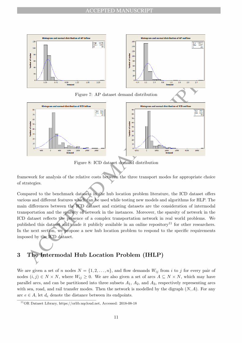
provide an analysis of the flow demand distribution for these different datasets. As shown in Figures 5-

8, the demand distributions in most cases are skewed due to the concentration of the demand flows

amongst a small subset of nodes. In other words, the flow demands have higher concentration in some

areas but less in many of the other areas. The example of this pattern can be seen from the AP dataset.

The flows of mail delivery to nodes that are close to the central business district are larger compared

to the nodes that are further away from the centre.

Table 2 gives an overview of flow demand concentrations between nodes with highest flow demands in

the CAB, AP, Turkey, and ICD datasets. Around 50% of the total demand is concentrated between

less than 25% of all nodes with highest flow demands in all cases except the Turkey dataset. Among

these four datasets, the ICD dataset has the most unbalanced demand distribution: nearly 80% of the

total demand is allocated to less than 40% of the nodes. In contrast to the case that the network is

fully connected and the transfer mode is uniform, the concentration of flow demands in a small portion

of nodes in the ICD dataset does not necessarily result in easier problems in general since the network

is sparse, and the high demand nodes may not be potential hubs.

Moreover, the distance matrix in the CAB, AP, and Turkey datasets are symmetric. In the CAB and

AP datasets, the geographical coordinates of nodes are given, and the distances are Euclidean distances

in the plane. However, due to traffic regulations and topological considerations, this assumption may

not be valid in practice. In sparse networks, we are more likely to encounter asymmetric distance

matrices because pairs of nodes are connected through intermediate nodes and links may have different

9

ACCEPTED MANUSCRIPT

ACCEPTED MANUSCRIP

T

Demandportion

CABAP

inflowAP

outflowTurkeyinflow

Turkeyoutflow

ICDinflow

ICDoutflow

50% 24.0 17.5 10.5 44.4 17.3 13.3 12.360% 32.0 24.5 17.0 54.3 24.7 19.0 16.970% 44.0 33.0 25.0 65.4 34.6 27.2 24.680% 60.0 43.0 37.0 76.5 46.9 39.0 37.4

Table 2: Demand concentration between high-demand nodes in a few HLP datasets

Figure 5: CAB demand distribution Figure 6: Turkey demand distribution

traffic when travel time is used for the selection of paths with different length. Note that, in this

context, an asymmetric distance matrix may also be realised in practice for a fully connected network.

In addition, the cost of a routing in the network is directly related to the distances of nodes and the cost

factors of the arcs that are used in the actual flow-routing. In the AP dataset, because of using distinct

transfer, collection and distribution cost factors, the cost matrix is asymmetric. Meanwhile, the CAB

and Turkey datasets have a symmetric cost matrix because of the application of the same collection

and distribution cost factors and the use of a symmetric distance matrix, which means only the travel

in one direction has to be considered. In the ICD dataset, different cost factors are associated with

different transfer modes. Also, since the distance matrix is asymmetric, the cost matrix is asymmetric.

Table 3 summarises the characteristics of these datasets. Note that the features of each dataset reflect

the characteristics of the corresponding original practical problem.

The flow demands in the ICD dataset are not evenly distributed through the regions of Indonesia. As

reported in 2009, a total of 8.8 million Twenty-foot Equivalent Unit (TEU) containers were handled

at Indonesian ports in total, 84% of which was concentrated in only 5 ports. These ports, located in

Java and Sumatera islands, are Tanjung Priok (3.9 million TEU), Tanjung Perak (1.7 million TEU),

Belawan (0.9 million TEU), Tanjung Emas (0.6 million TEU), and Panjang (0.3 million TEU) 10. There

is, thus, a high concentration of flow demand in a small number of ports. This has led to substantial

congestion on access roads near these ports because road transportation is mainly used for inland

transportation in Indonesia. Thus, most intermodal transport strategies encourage a greater usage of

the rail transport mode in order to ease road congestions. On the other hand, road transportation in

Indonesia currently enjoys fuel subsidies, which causes a reduction in the cost-competitiveness of rail

transportation. Increased rail transport is also expected to lead to environmental benefits and reduced

road accidents. Hence, there is a need for developing strategies, such as subsidising the utilisation

of rail, introducing new road pricing schemes, and road congestion taxes, in order to foster a more

competitive environment for more efficient intermodal transportations. The ICD dataset provides a

10Australian Aid-Indonesia Infrastructure Initiatives (IndII). Multimodal Transport Strategy: Java Corridor - FinalReport of Scoping Study, Technical Report, 2012.

10

ACCEPTED MANUSCRIPT

ACCEPTED MANUSCRIP

TFigure 7: AP dataset demand distribution

Figure 8: ICD dataset demand distribution

framework for analysis of the relative costs between the three transport modes for appropriate choice

of strategies.

Compared to the benchmark datasets in the hub location problem literature, the ICD dataset offers

various and different features which can be used while testing new models and algorithms for HLP. The

main differences between the ICD dataset and existing datasets are the consideration of intermodal

transportation and the sparsity of network in the instances. Moreover, the sparsity of network in the

ICD dataset reflects the presence of a complex transportation network in real world problems. We

published this dataset and made it publicly available in an online repository11 for other researchers.

In the next section, we propose a new hub location problem to respond to the specific requirements

imposed by the ICD dataset.

3 The Intermodal Hub Location Problem (IHLP)

We are given a set of n nodes N = {1, 2, . . . , n}, and flow demands Wij from i to j for every pair of

nodes (i, j) ∈ N × N , where Wij ≥ 0. We are also given a set of arcs A ⊆ N × N , which may have

parallel arcs, and can be partitioned into three subsets A1, A2, and A3, respectively representing arcs

with sea, road, and rail transfer modes. Then the network is modelled by the digraph (N,A). For any

arc e ∈ A, let de denote the distance between its endpoints.

11OR Dataset Library, https://orlib.uqcloud.net, Accessed: 2018-08-18

11

ACCEPTED MANUSCRIPT

ACCEPTED MANUSCRIP

T

DatasetFlow

demandNetwork

sizeCost

matrixDistancematrix

no.modes

Network Application

CAB Sym 25 Sym Sym 1 complete USA passenger airline networkAP Asym. 200 Asym. Sym. 1 complete Australia Post delivery systemTurkey ∼Sym. 81 Sym. Sym. 1 complete Turkey cargo delivery systemICD Asym. 225 Asym. Asym. 3 sparse Indonesian container distribution

Table 3: A comparison of a few hub location problem datasets

Any oriented path in the network connecting a pair of nodes can consist of arcs in A with different

modes. However, any two adjacent arcs in a path must be either in the same mode, or be incident to a

hub node. A hub is a node which facilitates a transfer mode interchange. A hub can be selected from

a given subset H ⊆ N of nodes. In other words H is a subset of nodes which represents the set of

potential hubs in the network. Changing the mode for each unit of flow incurs some cost. Furthermore,

the establishment of a node as a hub is only possible if a fixed cost is incurred. The problem of locating

a set of hubs among n nodes, and routing each flow demand with minimum total cost is called the

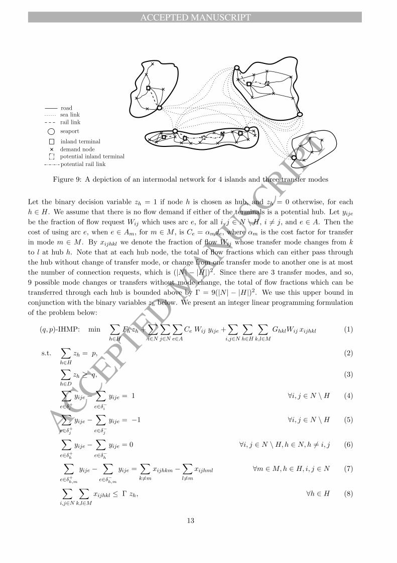
intermodal hub location problem (IHLP). Figure 9 illustrates an intermodal network for 4 islands with

three different transfer modes. Figure 9 also contains potential inland terminals and rail links. As we

discuss in Sections 4 and 5, we may include potential inland terminals and rail links in our dataset to

study the impact of network expansions.

In the IHLP, the number of located hubs, including seaports and inland terminals is to be decided in

such a way that the total cost is minimised. Inland terminals enable transfer between road and rail

while seaports provide transfer to ships. For a given pair of integers (q, p), where q ≤ p, the intermodal

multiple allocation hub location problem is one in which the total number of hubs is fixed to p and

the minimum number of inland terminals is set to q. We denote this problem as the (q, p)-intermodal

hub median problem ((q, p)-IHMP). As specified earlier, this problem is important for a few practical

reasons. At a strategic level, we use this model to understand the infrastructure budget that needs

to be allowed for capital and infrastructure works that are required to facilitate efficient container

flows in the network. We use this model to also understand the impact that various permutations of

inland terminals and seaports has on both traffic congestion as well as infrastructure costs. We expect

that there is a trade-off that needs to be struck between reduced congestion and costs of establishing

inland terminals. We expect to use this model to ascertain what the optimal balance is through the

provisioning of appropriate incentives that encourage rail transfers. We formulate and discuss this

particular problem in this paper from here on in, noting that there are many other interesting variants

of this problem that may also be explored. However, for the remainder of this paper we focus specifically

on the (q, p)-IHMP.

Mathematical formulation for (q, p)-IHMP

Let δ+i,m denote the subset of arcs with transfer mode m ∈M whose tails are i, and δ+i is the subset of

arcs whose tails are i, where M = {1, 2, 3}. In other words, δ+i,m = {e ∈ Am : e = (i, j) for some j ∈ N},for i ∈ N andm ∈M , and δ+i = ∪m∈Mδ+i,m. Analogously, define δ−i,m = {e ∈ Am : e = (j, i) for some j ∈N} and δ−i = ∪m∈Mδ−i,m. Denote by Ghkl the cost of changing transfer mode from k to l at hub h, for

each unit of flow and k, l ∈ M . Denote by Fh the cost of establishing node h as hub. We denote the

subset of inland terminal potential hubs by D, where D ⊂ H.

12

ACCEPTED MANUSCRIPT

ACCEPTED MANUSCRIP

T

roadsea linkrail link

seaport

inland terminal

demand node

potential rail link

potential inland terminal

Figure 9: A depiction of an intermodal network for 4 islands and three transfer modes

Let the binary decision variable zh = 1 if node h is chosen as hub, and zh = 0 otherwise, for each

h ∈ H. We assume that there is no flow demand if either of the terminals is a potential hub. Let yijebe the fraction of flow request Wij which uses arc e, for all i, j ∈ N \H, i 6= j, and e ∈ A. Then the

cost of using arc e, when e ∈ Am, for m ∈ M , is Ce = αmde, where αm is the cost factor for transfer

in mode m ∈ M . By xijhkl we denote the fraction of flow Wij whose transfer mode changes from k

to l at hub h. Note that at each hub node, the total of flow fractions which can either pass through

the hub without change of transfer mode, or change from one transfer mode to another one is at most

the number of connection requests, which is (|N | − |H|)2. Since there are 3 transfer modes, and so,

9 possible mode changes or transfers without mode change, the total of flow fractions which can be

transferred through each hub is bounded above by Γ = 9(|N | − |H|)2. We use this upper bound in

conjunction with the binary variables zh below. We present an integer linear programming formulation

of the problem below:

(q, p)-IHMP: min∑

h∈HFh zh +

∑

i∈N

∑

j∈N

∑

e∈ACe Wij yije +

∑

i,j∈N

∑

h∈H

∑

k,l∈MGhklWij xijhkl (1)

s.t.∑

h∈Hzh = p, (2)

∑

h∈Dzh ≥ q, (3)

∑

e∈δ+i

yije −∑

e∈δ−i

yije = 1 ∀i, j ∈ N \H (4)

∑

e∈δ+j

yije −∑

e∈δ−j

yije = −1 ∀i, j ∈ N \H (5)

∑

e∈δ+h

yije −∑

e∈δ−h

yije = 0 ∀i, j ∈ N \H,h ∈ N,h 6= i, j (6)

∑

e∈δ+h,m

yije −∑

e∈δ−h,m

yije =∑

k 6=mxijhkm −

∑

l 6=mxijhml ∀m ∈M,h ∈ H, i, j ∈ N (7)

∑

i,j∈N

∑

k,l∈Mxijhkl ≤ Γ zh, ∀h ∈ H (8)

13

ACCEPTED MANUSCRIPT

ACCEPTED MANUSCRIP

T

zh ∈ {0, 1}, xijhkl ≥ 0, yije ≥ 0 ∀i, j ∈ N,h ∈ H, k, l ∈M, e ∈ A. (9)

Equation (2) fixes the number of located hubs to p, and equation (3) ensures that the required minimum

number of inland terminals are located. The equations (4)-(6) are flow conservation constraints for flow

between demand nodes. Equations (4) and (5) ensure that the total flow for any flow demand is

sourced and terminated at corresponding terminals, and the set of constraints (6) ensures that inflow

and outflow of a demand at any intermediate node are equal. Through the set of constrains (7), xijhklcaptures the exact amount of flow portion for demand (i, j) which changes transfer mode from k to l

at hub h, for all i, j ∈ N, k, l ∈ M , and h ∈ H. The right term of constraints (7) gives the increased

fraction of flow Wij in transfer mode m at hub h. In (7), for a fixed (i, j) and h, there are |M | equations

and |M |(|M | − 1) variables xijhkl (we already excluded xijhmm for m ∈ M). In any optimal solution,

at most |M |(|M | − 1)/2 of these variables are positive. When |M | = 3, the set of equations in (7) has

a unique solution for the variables xijhkl for fixed yije for e ∈ A. Thus xijhkl captures the fraction of

Wij with mode change from k to l at hub h in any feasible solution. From xijhkl we can assess the

congestion at links incident to hubs in different modes, and congestion at facilities for transfer mode

changes. The set of constraints (8) guarantees that all mode changes only occur at the selected hubs.

This constraint can be disaggregated to create a tighter but larger formulation. Finally, the objective

function reflects the total cost of fulfilling flow demands. The cost of locating hubs, the cost of flow

through links, and the cost of transfer mode changing in all paths are respectively considered in the

first, second and third terms of (1).

Note that (1)-(9) provides a rigorous and straightforward mathematical formulation for (q, p)-IHMP,

which differs from the existing formulations in the literature (for example, see Ishfaq and Sox (2011);

Arnold et al. (2004)) in several ways. Our formulation allows three distinct transfer modes and the

transfer mode changes at hubs, and relaxes the full-connectivity assumption for the hub network.

Our formulation is partly based on the original hub location formulations, and partly based on the

choice of variables xijhkl, which bring about these advantages. But the number of variables in (q, p)-

IHMP remains in the same order as in existing formulations for the hub location problems. When the

underlying network is sparse, the number of arcs can be considered to be of linear order in the number

of nodes, that is |A| = O(n). The number of origin destination pairs is at most O(n2). In formulation

(1)-(9), the number of binary variables is |H|, the number of real variables is O(n3), and the number of

constraints is O(n3). Interestingly, for any feasible set of p hubs by which a path for every flow demand

exists in the network, there is an optimal solution in which the real variables yije and xijhkl are either

0 or 1. In fact, if there are two fractional flow paths between two nodes (i, j), say P1 and P2, then we

can always choose the cheaper path since there is no capacity on links/nodes. If the total cost of one

of them is larger, then the fraction of flow through that path is zero. If P1 and P2 have the same cost,

then either of them can be chosen to have zero flow. Hence, since the coefficients of all variables in the

objective function are positive, there is an optimal solution in which all variables have integer values.

Theorem 3.1. (q, p)-IHMP is NP-hard.

Proof. To prove this claim, we show that a given instance of UMApHMP can be reduced to an instance

of (q, p)-IHMP. Since the p-hub median problems are NP-hard (Love et al., 1988), this reduction proves

that (q, p)-IHMP is NP-hard. Suppose we are given an instance of symmetric UMApHMP, denoted by

14

ACCEPTED MANUSCRIPT

ACCEPTED MANUSCRIP

T

P1, on the set of nodes {1, 2, . . . , n} to locate p hubs, in which Wij is the flow request for pair (i, j),

and dij is the distance between i and j. Let N = {1, 2, . . . , n} × {0, 1}, and let A be the set of arcs

{((i, 0), (j, 1)), ((i, 1), (j, 0)), ((i, 1), (j, 1)) : i, j = 1, 2, . . . , n, i 6= j}. Now we construct a network on the

set of nodes N and the set of arcs A. Any arc ((i, 0), (j, 1)) or ((i, 1), (j, 0)) is considered to be in mode

2, and any arc ((i, 1), (j, 1)) is considered to be in mode 3, where i, j = 1, 2, . . . , n. This network does

not contain any arc in mode 1. Then we construct P2, an instance of (q, p)-IHMP, in which q = 0 and

the set of potential hubs H is the set of nodes {(i, 1) : i = 1, 2, . . . , n} (see Figure 10 for an illustration).

We set the flow demands for ((i, oi), (j, oj)) to be Wij if oi = oj = 0, and zero otherwise. Moreover, we

set the distance of (i, oi) and (j, oj) to be dij , for oi, oj ∈ {0, 1}, and (oi, oj) 6= (0, 0). We set mode cost

factors α2 to be the collection/distribution factor, and α3 to be the transfer cost between hubs in P1.

We set the cost of change modes and installation fixed costs to zero in P2.

(i, 1)

(i, 0)

(j, 1)

(j, 0)

Figure 10: Construction of a (q, p)-IHMP instance from a UMApHMP instance

We show that any optimal solution of P1 corresponds to an optimal solution of P2 with the same

optimal value, and vice versa. For a given feasible solution of P1, suppose {kt : t = 1, 2, . . . , p} is the

set of located hubs, and (ksij)s is the ordered visited hubs on the route from i to j. This is equivalent

to a solution of P2, in which {(kt, 1) : t = 1, 2, . . . , p} is the set of located hubs. Moreover, there is a

route from (i, 0) to (j, 0) which visits hubs ((ksij , 1))s in order. It is obvious that the cost of the two

path in P1 and P2 are the same.

On the other hand, clearly any set of p hubs in P2 gives rise to a set of p hubs in P1. Suppose

Pij = (i, 0), (k1, o1), . . . , (kt, ot), (j, 0) is the shortest path in P2 between (i, 0) and (j, 0). Note that

ol = 1 for l = 1, 2, . . . , t. Otherwise the path (i, 0), (k1, 1), . . . , (kt, 1), (j, 0) is less expensive than Pij .

Then i, k1, . . . , kt, j is an equivalent path of Pij in P1 with the same cost. Therefore, any optimal

solution of P1 corresponds to an optimal solution of P2 with the same cost, and vice versa. This

completes the proof.

The (q, p)-IHMP is an interesting extension of the traditional hub location problem for intermodal

versions. In (q, p)-IHMP, (a) hubs serve consolidations/unconsolidations of goods and facilitate transfer

mode changes, and (b) two types of hubs are distinguished so that any requirement for prioritising the

installation of one type of hub can be accommodated. A similar discussion holds for the IHLP, in which

the optimal number of hubs is determined by optimal solutions. A formulation for IHLP can be obtained

from the (q, p)-IHMP formulation by dropping (2) and (3). However, IHLP and (q, p)-IHMP are only

15

ACCEPTED MANUSCRIPT

ACCEPTED MANUSCRIP

T

two of many possible extensions of the traditional hub location problems in the intermodal networks.

Other extensions, including the capacitated hub location problem (see Ernst and Krishnamoorthy

(1999)), single allocation problem (see Ernst and Krishnamoorthy (1996)), and hub center problem

(see Ernst et al. (2009)) could be explored. We leave these investigations for the future.

In the following we use a commercial solver to solve instances of (q, p)-IHMP and analyse the solutions

thus produced. Due to computational restrictions, we are not able to solve the very large problem

instances. Because of the inherent complex nature of (q, p)-IHMP we can borrow from the literature

on traditional hub location problems, and employ many effective approaches for solving the problem.

These would include heuristics (see Ernst and Krishnamoorthy (1998b)) and Benders decomposition

(see Mokhtar et al. (a,b,c)). Future research should explore these approaches for solving larger instances

of (q, p)-IHMP efficiently. In our current work, we wished to motivate our research, indicate why new

models were required, present a new dataset, provide a formulation for the new problem, provide initial

computational results to simply demonstrate what sorts of analyses could be carried out, and present

our computational analysis. In the next sections, we present our computational results using CPLEX

and the analyse these results.

4 Computational Results

In this section we present extensive computational results of our experiments on the ICD dataset and

intermodal hub location problems 11. We consider different scenarios in which the cost factors, or the

network structure in the ICD dataset is modified. We then analyse our computational results using

different scenarios in Section 5. We show how inland terminals, congestion taxes and rail subsidies can

actually improve intermodal network flow and reduce road congestion in large cities. In Table 4, we

first summarise the notations that we will use throughout this section.

notation description

time the computational time in secondsObj the optimal value of objective function divided by 1.0e13πs number of 100,000 containers routed through sea linksπd number of 100,000 containers routed through road links incident to seaports with rail terminalsπl number of 100,000 routed through rail links incident to seaports with rail terminalsRR% percentage of containers routed through road links incident to seaports with rail terminalsd<>l number of 100,000 containers interchanged modes between road and rail at a seaport with rail terminald<>s number of 100,000 containers interchanged modes between sea and road at a seaport with rail terminall<>s number of 100,000 containers interchanged modes between sea and rail at a seaport with rail terminal

Table 4: Notations used in computational results

All computations were performed on a computer with 8 cores of 2.5 GHz processors and 32 Gb

memory, with 64-bit Linux RedHat operating system. All methods were coded in C++ using the

Concert Technology CPLEX 12.6. To improve computational efficiency, we set a few parameters in

CPLEX empirically, based on limited numerical experiments with small instances. We set the rule for

selecting the branching variable to be based on pseudo-shadow prices, and the solution algorithm at

root nodes to be the dual simplex method. We also switched off the usage of ‘heuristic in nodes’. The

time limit for all computations was fixed to 7200 seconds. If within the specified time limit, a method

is able to find the optimal solution, the corresponding CPU time is presented in seconds (sec). If the

16

ACCEPTED MANUSCRIPT

ACCEPTED MANUSCRIP

T

Figure 11: An optimal solution for the instance with n = 73, p = 12, q = 4 (road links are not shown)

method only finds a feasible non-optimal solution, the gap between the best solution is presented in

the ‘time’ column.

We present our computational results for (q, p)-IHMP for the ICD dataset in Tables 6 and 7. Since

the instances on 53 nodes are not representative of distribution for demand nodes in the high demand

area Java, we have only present results on instances with more than 60 nodes. The largest instance

we could solve optimally with our settings was the 73-node instance. An optimal location of hubs and

inland terminals for an instance with 73 nodes is illustrated in Figure 11. In fact, we experimented

our program on instances with 97 nodes or more with the 3-hour time limit. In most cases, no feasible

solution was found, and in a few cases, the quality of solutions were not satisfactory for presentation

here. Over the last two decades the hub location research community has made significant progress in

solving larger instances, in part due to the challenge provided by larger realistic data sets such as the

Australia Post and Turkey datasets. This paper is in part providing a similar challenge to push the

boundaries of what problems can be solved in the hub location area. Also, there are many ways to

extend the computational experiments and analyse solutions. We believe that further research, newer

algorithms and more experiments will be needed to solve these larger problem instances more effectively.

In the archipelago of Indonesia, there are five main islands which can only be connected thorough sea

links. Therefore, p ≥ 5 and q ranges between 0 and p − 5. Note that for p larger than the number

of potential seaports, at least p − k inland terminals are already included, where k is the number of

seaports. Therefore, problems with q = 0, 1, . . . , p − k are equivalent. Thus, we only consider one of

the equivalent problems in our computational experiment.

Congestion along roads that lead to seaports is a major issue in Indonesia7. Thus, we analyse the

number of containers transferred to seaports through road links, either for shipping, loading trains, or

bypassing seaports. Tables 6 and 7 respectively present our computational results for instances with 66

and 73 nodes respectively. In the first scenario, the original pricing of all modes are used (see Section 2).

17

ACCEPTED MANUSCRIPT

ACCEPTED MANUSCRIP

T

scenario/cost factors sea links road links rail links

ICD, ICD+10%, ICD+25% 5.47 12.98 3.92ICD-66%-discnt 5.47 12.98 1.3044ICD-99%-discnt 5.47 12.98 0.0392

Table 5: Cost factors of different modes in different scenarios

In scenarios ICD-66%-discnt and ICD-99%-discnt, respectively, the pricing of train transportation is

discounted by 66% and 99%, respectively (see Table 5). Of course ICD-99%-discnt is not a realistic

scenario. So, we use it only for the purpose of analysis. The corresponding results are presented in the

columns ICD-66% and ICD-99% in Tables 6 and 7. Also we assess the effect of increasing the number

of rail links too. We add more rail links to the existing rail network to the 10%, and 25% highest

demand nodes (explained later). Since the rail network in Indonesia is very sparse, these scenarios are

helpful in the analysis of the impact of the rail network expansion on throughput and congestion. The

corresponding results are presented in the columns ICD+10% and ICD+25% in Tables 6 and 7 respectively

(where we were able to solve the instances). In total, our computational experiments are performed on

680 instances. All computation results are available in an online repository 11.

As shown in Tables 6 and 7, the computational time for (q, p)-IHMP increases with the number of

nodes because of the sharp increase in the number of variables in the model. Generally, there is an

increase in the computational effort as p decreases and n, q are fixed, or when q increases and n, p are

fixed (due to more intense competitions for the location of hubs). Also, for smaller differences of p

and q (that is p − q), the computational effort surges because of the high competition for resolving

potential hub locations. As the number of p-hub combinations increase, the search space grows and the

computational effort increases. For fixed n and increasing p, the fixed costs increase and the network

flow costs decreases (since flow costs dominate the fixed costs) and the objective value decreases as p

increases. For fixed (n, p), the feasible set of the problem shrinks as q grows, and the objective value

increases. Intuitively, with larger q, there is a tougher competition between seaports (and also inland

terminals) to be chosen, and hence the computational time increases in general. In most cases, the

computational effort is dominated by these trade-offs.

In Tables 6 and 7, the number of containers routed through road links incident to some seaport which

have rail terminals, indicated by πd, has a decreasing trend as q grows and p or p−q are fixed in general.

This is due to the presence of more inland terminals and deviation of transportations from seaports to

inland terminals. It is interesting that very few inland (rail only) hubs are selected by the model. The

first time that this happens is for p = 12, as can be seen by the fact that the cost does not increase

when the use of an inland terminal is forced (q = 1). d<>s, πd and πl demonstrate the usage of road

for sea transfer, the road congestion and usage of trains respectively. d<>s and πd decrease while πlgrows as q increases and p− q is fixed in general (see Figures 14-18).

When the number of inland hubs is small, seaports are used not only for shipping through sea links,

but also for change of transfer modes between road and rail. It can be observed from Tables 6 and

7 that for larger numbers of inland hubs, that is q ≥ 3 and p ≤ 11, there is a significant drop in the

volume of πd, πl, and d<>l. This is justified by the smaller number of containers that change mode

to sea using roads and more usage of inland terminals to change mode between land modes instead of

using seaport facilities. This observation can also be a signal to the significant importance of inland

18

ACCEPTED MANUSCRIPT

ACCEPTED MANUSCRIP

T

terminals in (q, p)-IHMP. When the number of inland terminals is small (generally when q is small),

a larger number of transfer mode interchanges to sea are delivered by trucks, and seaports play the

role of inland terminals to facilitate the interchange between land modes, especially for routes between

nodes in the same island. There are cases in which a few seaports in the optimal solutions are solely

used to facilitate d<>l interchanges. Note that in many instances with q ≤ 2, inland hubs are mostly

used for transportation between two parts of large demand nodes rather than facilitating transfer of

containers to seaports. For q ≥ 3, there are a few inland terminals which have direct rail links to some

seaports. Thus, such inland terminals support a cheaper transfer of containers to seaports. As a result,

road congestion at seaports is also avoided. This leads us to a conclusion that the installation of inland

terminals can help easing the traffic congestions at seaport roads, and a more comprehensive utilisation

of infrastructure at seaports for sea shipments (as a result of capacity-reduction inducing queuing) at

seaports for shipments through sea links.

For the scenarios with discounted rail costs, we make similar observations to those in the above para-

graphs. In both scenarios ICD-66%-discnt and ICD-99%-discnt, a larger number of inland terminals

– up to the case when q ≤ p − 6 – causes reductions in congestion at seaport roads and the number

of interchange of modes at seaports. Due to less expensive train transportation, the transportation

through seaport by roads decreases from over 46% to about 34% in ICD-66%-discnt on average. Using

the ICD-99%-discnt scenario, we obtain a lower bound on the number of containers routed through

road, and interchanges at seaports in this given network structure.

In our experiments, we further included more rail links to analyse how a denser rail network could

help the network flow in this problem since the number of rail links in Indonesia is quite small. We

considered demand nodes with the highest flow amounts in the network which contribute to 10% of

total flow in the problem. An inland terminal for each of such demand nodes is added. Then we

added a tree of rail links to connect potential hubs. We repeated the same procedure for demand nodes

with highest flow amounts contributing to 25% of total containers. We denote these two scenarios by

ICD+10% and ICD+25% respectively.

In these two experiments, the total rail and road transportations and d<>s at seaports reduces, while

the portion of rail transportation and l<>s increases. In scenarios with more rail links or discounted

train transportation, the usage of trains is enhanced. However, a larger portion of demands in the

scenarios with new rail links are fulfilled by trains which reduced the usage of trucks at seaports in

general.

There are many interesting variations of IHLP and, in particular (q, p)-IHMP. We leave the exploration

of these variants for subsequent work on this topic. One interesting variant of (q, p)-IHMP is one in

which the number of hubs is not fixed. We get a different intermodal hub location problem when we

consider this option.

In this free-hubs variant of (q, p)-IHMP, the optimal number of hubs is left to be determined by the

optimisation based on fixed costs for hubs. We also experiment with this version of the intermodal hub

location problem, and present the computational results in Table 8. The number of tested instances for

this variation is smaller since the argument on experimentation for different combinations of p and q is

not valid. In this table, computational results on instances with 66 and 73 nodes are presented to be

19

ACCEPTED MANUSCRIPT

ACCEPTED MANUSCRIP

T

ICD ICD-66% ICD-99% ICD+10% ICD+25%

p q time Obj πs πd πl RR% d<>l d<>s l<>s time Obj πs πd πl RR% d<>l d<>s l<>s time Obj πs πd πl RR% d<>l d<>s l<>s time Obj πs πd πl RR% d<>l d<>s l<>s time Obj πs πd πl RR% d<>l d<>s l<>s

5 0 8% 19.0 107 66 0 100% 35 31 35 t 16% 19.5 95 66 0 100% 35 31 35 t t6 0 4000 17.1 101 87 58 60% 61 26 50 7116 16.5 101 94 69 58% 69 26 51 3% 16.3 101 98 74 57% 72 26 51 5964 14.9 61 87 80 52% 80 7 31 7% 15.6 59 87 74 54% 80 7 27

1 20% 21.2 92 68 32 68% 40 28 38 t t 6494 15.1 59 60 48 56% 52 8 25 t 0.07 0 2% 16.3 99 87 53 62% 60 27 47 2% 15.8 100 94 68 58% 69 26 49 6830 15.5 100 98 72 58% 73 26 49 1% 14.1 61 87 77 53% 80 7 29 1% 14.2 61 87 77 53% 80 7 29

1 3% 16.8 98 88 88 50% 63 25 49 4% 16.2 101 101 85 54% 77 25 52 t 5491 14.3 59 60 48 56% 52 8 25 2% 14.5 59 60 48 56% 53 8 252 t 9% 17.5 90 60 44 58% 35 25 41 6% 16.5 107 60 38 61% 37 23 43 t t 0.0

8 0 4919 15.6 99 80 53 60% 58 21 45 5304 15.1 100 87 68 56% 67 20 47 3537 14.8 100 92 75 55% 68 25 50 4493 13.6 68 113 127 47% 107 6 30 3213 13.7 68 113 127 47% 107 6 301 2% 15.9 99 88 64 58% 63 25 49 4% 15.6 100 73 84 46% 68 5 41 2832 14.8 100 92 75 55% 68 25 50 2% 13.8 65 82 91 48% 77 5 28 3243 13.8 65 82 91 48% 77 5 282 4691 16.5 101 91 81 53% 67 24 53 5950 15.7 101 95 86 52% 71 24 53 4597 15.2 101 94 87 52% 70 24 53 6709 13.9 59 57 54 51% 52 5 27 t 0.03 6711 17.3 107 60 44 58% 35 25 41 6266 16.5 107 64 51 55% 42 22 44 5% 16.1 107 62 53 54% 41 22 45 5877 14.5 59 57 54 51% 52 5 27 5348 14.6 59 57 54 51% 52 5 27

9 0 668 15.1 109 106 115 48% 85 20 46 1674 14.5 100 112 141 44% 92 20 48 2097 14.2 100 85 75 53% 66 19 48 1617 13.3 68 116 133 47% 111 5 32 3339 13.4 68 116 133 47% 111 5 321 2695 15.3 99 81 64 56% 61 20 47 4170 14.6 100 86 73 54% 66 20 48 3739 14.2 100 85 75 53% 66 19 48 2765 13.3 68 116 133 47% 111 5 32 6017 13.4 68 116 133 47% 111 5 322 6896 15.7 99 91 77 54% 67 24 50 3332 14.9 100 95 85 53% 71 24 51 3283 14.5 100 94 86 52% 70 23 52 4987 13.4 61 90 91 50% 86 4 32 1628 13.5 61 90 91 50% 86 4 323 4% 16.4 101 86 90 49% 63 23 54 4197 15.5 101 90 96 48% 67 23 54 3% 15.2 101 74 144 34% 67 7 69 4% 14.0 74 38 85 31% 33 5 28 3875 13.8 59 57 54 51% 52 5 274 t 7097 16.5 107 44 77 36% 38 6 60 10% 16.7 90 54 61 47% 38 16 50 3083 14.3 59 52 61 46% 48 3 29 5166 14.5 59 52 61 46% 48 3 29

10 0 474 14.8 109 109 127 46% 89 19 48 1808 14.2 100 114 153 43% 95 19 49 1521 13.8 100 87 86 50% 68 18 50 724 13.0 68 120 138 46% 115 5 32 909 13.1 68 120 155 44% 115 5 321 603 14.8 109 109 127 46% 89 19 48 696 14.2 100 114 153 43% 95 19 49 4277 13.8 100 87 86 50% 68 18 50 1545 13.0 68 120 138 46% 115 5 32 2106 13.1 68 120 155 44% 115 5 322 2119 15.0 99 84 77 52% 65 19 48 1291 14.2 100 87 85 51% 69 18 49 785 13.8 100 87 86 50% 68 18 50 1159 13.1 68 111 140 44% 108 3 33 2634 13.3 61 94 114 45% 90 4 323 6561 15.5 99 86 86 50% 63 23 51 5819 14.7 100 90 94 49% 68 23 52 6613 14.3 100 89 95 48% 67 22 53 1438 13.3 61 85 99 46% 82 3 33 4134 13.4 61 85 99 46% 82 3 334 5% 16.6 150 39 62 39% 31 9 50 4209 15.4 101 70 121 37% 64 6 70 3273 14.9 101 70 123 36% 63 6 70 3151 13.6 59 52 61 46% 48 3 29 2046 13.7 59 52 61 46% 48 3 295 3658 17.2 107 51 51 50% 32 19 47 6173 16.5 107 38 74 34% 33 6 61 3321 16.0 107 43 79 35% 38 6 61 3315 14.2 59 32 86 27% 28 3 29 1971 14.4 59 31 69 31% 28 3 29

11 0 492 14.6 109 113 136 45% 95 18 49 371 13.9 100 118 161 42% 101 17 50 704 13.5 100 91 94 49% 74 17 51 279 12.8 69 118 138 46% 113 5 30 456 12.9 69 120 155 44% 115 5 321 342 14.6 109 113 136 45% 95 18 49 325 13.9 100 118 161 42% 101 17 50 1040 13.5 100 91 94 49% 74 17 51 386 12.8 69 118 138 46% 113 5 30 320 12.9 69 120 155 44% 115 5 322 1047 14.7 109 104 136 43% 86 18 49 1329 14.0 100 91 93 50% 74 17 51 807 13.5 100 91 94 49% 74 17 51 1522 12.9 68 115 145 44% 112 3 33 1272 13.0 68 115 162 42% 112 3 333 1760 14.9 99 79 86 48% 61 18 49 2242 14.1 100 83 94 47% 66 17 50 2288 13.7 100 82 95 46% 65 17 51 3718 13.0 68 91 164 36% 87 3 33 1934 13.1 61 89 121 42% 86 3 334 3258 15.5 99 66 111 37% 59 7 67 4514 14.6 100 70 120 37% 64 6 69 2547 14.2 100 70 121 36% 63 6 69 691 13.2 61 65 123 34% 61 3 33 3019 13.3 61 65 107 38% 61 3 335 2879 16.3 101 55 108 34% 48 6 70 3203 15.4 101 65 118 36% 59 6 70 3816 14.9 101 70 123 36% 64 6 70 1987 13.5 59 32 86 27% 28 3 29 3964 13.7 59 31 69 31% 28 3 29

12 0 561 14.5 109 108 144 43% 91 17 50 891 13.8 100 114 170 40% 98 16 51 1054 13.3 100 113 177 39% 97 17 51 500 12.7 69 113 145 44% 110 4 31 452 12.8 69 115 162 42% 112 4 331 562 14.5 109 108 144 43% 91 17 50 527 13.8 100 114 170 40% 98 16 51 834 13.3 100 113 177 39% 97 17 51 382 12.7 69 113 145 44% 110 4 31 698 12.8 69 115 162 42% 112 4 332 427 14.5 109 108 144 43% 91 17 50 1556 13.8 100 114 170 40% 98 16 51 2027 13.3 100 113 177 39% 97 17 51 376 12.7 69 113 145 44% 110 4 31 460 12.8 69 115 162 42% 112 4 333 839 14.6 152 90 154 37% 83 7 60 1026 13.8 100 87 103 46% 71 16 52 690 13.3 100 86 104 45% 70 16 52 781 12.8 67 108 143 43% 105 3 33 1158 12.9 67 108 160 40% 105 3 334 1426 14.9 142 65 105 38% 59 7 60 767 14.0 143 70 113 38% 63 6 61 569 13.5 143 69 115 38% 63 6 62 868 12.9 67 84 162 34% 81 3 33 1018 13.1 64 75 118 39% 72 3 305 1765 15.5 99 55 104 35% 48 6 68 1056 14.6 100 65 117 36% 59 6 69 1099 14.2 100 70 122 37% 64 6 69 784 13.1 64 50 120 30% 47 3 30 1554 13.3 64 50 103 33% 47 3 30

13 0 257 14.4 108 108 145 43% 91 17 50 597 13.6 100 108 183 37% 92 16 52 760 13.1 100 109 186 37% 93 16 52 473 12.6 69 113 146 44% 110 4 31 426 12.7 69 115 162 42% 112 4 331 274 14.4 108 108 145 43% 91 17 50 708 13.6 100 108 183 37% 92 16 52 751 13.1 100 109 186 37% 93 16 52 789 12.6 69 113 146 44% 110 4 31 922 12.7 69 115 162 42% 112 4 332 255 14.4 108 108 145 43% 91 17 50 473 13.6 100 108 183 37% 92 16 52 767 13.1 100 109 186 37% 93 16 52 756 12.6 69 113 146 44% 110 4 31 763 12.7 69 115 162 42% 112 4 333 595 14.4 108 104 144 42% 88 16 51 463 13.6 100 108 183 37% 92 16 52 501 13.1 100 109 186 37% 93 16 52 937 12.6 68 106 143 43% 103 3 31 519 12.7 68 109 159 41% 105 3 344 651 14.6 151 86 154 36% 79 7 60 820 13.7 143 72 122 37% 67 5 63 659 13.3 143 71 123 37% 66 5 63 1004 12.7 82 83 161 34% 80 3 31 987 12.9 67 86 166 34% 83 3 335 643 14.9 142 54 97 36% 48 6 60 885 14.0 143 65 110 37% 59 6 62 456 13.5 143 69 115 38% 63 6 62 587 12.9 78 50 119 30% 46 3 28 973 13.0 64 60 112 35% 57 3 30

14 0 385 14.3 108 108 146 43% 91 17 50 390 13.5 100 108 183 37% 92 16 52 426 13.0 100 109 186 37% 93 16 52 374 12.5 67 106 143 43% 103 3 31 347 12.6 67 109 160 40% 105 3 341 247 14.3 108 108 146 43% 91 17 50 337 13.5 100 108 183 37% 92 16 52 398 13.0 100 109 186 37% 93 16 52 518 12.5 67 106 143 43% 103 3 31 616 12.6 67 109 160 40% 105 3 342 264 14.3 108 108 146 43% 91 17 50 1170 13.5 100 108 183 37% 92 16 52 528 13.0 100 109 186 37% 93 16 52 751 12.5 67 106 143 43% 103 3 31 945 12.6 67 109 160 40% 105 3 343 374 14.3 107 104 145 42% 88 16 51 419 13.5 100 108 183 37% 92 16 52 627 13.0 100 109 186 37% 93 16 52 407 12.5 67 106 143 43% 103 3 31 276 12.6 67 109 160 40% 105 3 344 393 14.4 151 88 163 35% 83 5 62 434 13.5 143 93 202 32% 88 5 63 653 13.0 143 94 205 31% 89 5 63 559 12.5 82 86 169 34% 82 3 31 400 12.6 82 88 165 35% 85 3 345 518 14.6 151 75 144 34% 69 7 60 673 13.7 143 67 119 36% 62 5 63 439 13.2 143 71 123 37% 67 5 63 548 12.7 78 52 127 29% 49 3 28 682 12.8 64 60 112 35% 57 3 30

15 1 295 14.2 119 111 151 42% 94 17 50 451 13.4 101 108 183 37% 92 16 52 449 13.0 143 94 206 31% 89 5 63 1136 12.4 81 86 170 34% 82 3 31 261 12.5 67 109 160 40% 105 3 342 204 14.2 119 111 151 42% 94 17 50 494 13.4 101 108 183 37% 92 16 52 2096 13.0 143 94 206 31% 89 5 63 823 12.4 81 86 170 34% 82 3 31 443 12.5 67 109 160 40% 105 3 343 288 14.2 107 104 146 42% 88 16 51 506 13.4 101 108 183 37% 92 16 52 2658 13.0 143 94 206 31% 89 5 63 447 12.4 81 86 170 34% 82 3 31 353 12.5 67 109 160 40% 105 3 344 234 14.3 150 88 164 35% 83 5 62 316 13.4 143 93 202 32% 88 5 63 190 13.0 143 94 206 31% 89 5 63 270 12.4 81 86 170 34% 82 3 31 775 12.6 81 88 166 35% 85 3 345 277 14.4 151 78 153 34% 73 5 62 431 13.5 143 88 197 31% 84 5 63 363 13.0 143 94 205 31% 89 5 63 479 12.5 82 74 158 32% 71 3 31 407 12.6 82 77 154 33% 73 3 34

16 2 391 14.2 118 107 151 41% 91 16 51 256 13.4 144 93 202 32% 88 5 63 154 12.9 144 94 206 31% 89 5 63 173 12.4 81 86 170 33% 82 3 31 105 12.5 71 111 180 38% 108 3 343 626 14.2 118 107 151 41% 91 16 51 225 13.4 144 93 202 32% 88 5 63 125 12.9 144 94 206 31% 89 5 63 74 12.4 81 86 170 33% 82 3 31 117 12.5 71 111 180 38% 108 3 344 402 14.2 150 88 165 35% 83 5 62 70 13.4 144 93 202 32% 88 5 63 66 12.9 144 94 206 31% 89 5 63 110 12.4 81 86 170 33% 82 3 31 116 12.5 81 88 166 35% 85 3 345 179 14.3 150 78 153 34% 73 5 62 301 13.4 143 88 197 31% 84 5 63 198 13.0 143 94 206 31% 89 5 63 202 12.4 81 74 158 32% 71 3 31 426 12.5 81 77 154 33% 73 3 34

17 3 314 14.2 118 101 152 40% 87 14 53 227 13.3 117 108 191 36% 94 14 54 226 12.9 144 109 221 33% 104 5 63 554 12.3 71 90 166 35% 87 3 31 264 12.4 71 99 174 36% 96 3 344 260 14.2 118 101 152 40% 87 14 53 146 13.3 117 108 191 36% 94 14 54 212 12.9 144 109 221 33% 104 5 63 119 12.3 71 90 166 35% 87 3 31 505 12.4 71 99 174 36% 96 3 345 242 14.2 150 78 154 34% 73 5 62 204 13.4 144 88 197 31% 84 5 63 239 12.9 144 94 206 31% 89 5 63 124 12.3 81 74 159 32% 71 3 31 200 12.5 81 77 155 33% 73 3 34

18 4 91 14.2 118 91 141 39% 77 14 53 92 13.3 117 108 217 33% 94 14 54 219 12.9 144 109 247 31% 104 5 63 110 12.3 71 78 155 34% 75 3 31 198 12.4 71 88 163 35% 85 3 345 179 14.2 118 91 141 39% 77 14 53 85 13.3 117 104 187 36% 90 14 54 190 12.9 144 109 221 33% 104 5 63 93 12.3 71 78 155 34% 75 3 31 57 12.4 71 88 163 35% 85 3 34

19 5 17 14.2 118 91 141 39% 77 14 53 17 13.3 117 104 212 33% 90 14 54 25 12.9 144 109 247 31% 104 5 63 222 12.3 71 78 166 32% 75 3 31 107 12.4 71 88 176 33% 85 3 34

Table 6: Computational results on the ICD dataset for n = 6620

ACCEPTED MANUSCRIPT

ACCEPTED MANUSCRIP

T

ICD ICD-66% ICD-99% ICD+10%

p q time Obj πs πd πl RR% d<>l d<>s l<>s time Obj πs πd πl RR% d<>l d<>s l<>s time Obj πs πd πl RR% d<>l d<>s l<>s time Obj πs πd πl RR% d<>l d<>s l<>s

5 0 9.95% 19.8 111 68 0 100% 36 32 36 t t t6 0 6033 17.7 106 89 60 60% 62 27 53 17.58% 19.9 95 64 32 67% 39 25 43 16% 19.3 95 38 36 51% 30 8 31 6898 15.5 66 89 83 52% 82 7 33

1 14.31% 20.2 97 67 14 82% 38 28 40 14.31% 19.7 111 62 28 69% 37 25 43 22% 20.8 95 48 28 63% 34 15 53 5550 15.7 63 62 49 56% 54 8 277 0 5253 16.9 104 89 55 62% 62 27 50 2.56% 16.6 106 123 153 44% 97 26 54 4% 16.2 105 72 75 49% 66 6 42 5987 14.7 66 89 80 53% 82 7 31

1 7148 17.4 106 91 72 56% 65 26 54 3.80% 16.6 106 94 77 55% 69 25 54 3% 16.2 106 94 79 54% 69 25 54 4445 14.9 64 62 49 56% 54 8 272 6.02% 18.6 95 60 48 56% 35 25 43 t 6% 17.4 99 62 45 58% 36 26 42 7217 15.8 61 59 56 51% 53 6 29

8 0 3594 16.2 105 82 55 60% 60 22 48 5197 15.7 105 90 70 56% 69 21 49 5311 15.4 105 94 75 56% 73 21 49 4291 14.2 73 116 131 47% 110 6 321 6339 16.5 104 91 67 57% 65 26 51 5023 15.8 105 94 75 56% 69 25 52 5534 15.4 105 94 77 55% 69 25 53 4344 14.3 69 85 94 48% 80 5 302 6849 17.1 106 95 84 53% 70 25 55 3.11% 16.4 106 68 88 44% 64 4 46 6451 15.9 106 97 90 52% 73 24 55 6470 14.5 64 59 56 51% 53 6 293 9.23% 18.6 95 59 42 58% 33 26 42 6063 17.2 111 66 52 56% 44 23 46 6506 16.7 111 65 54 55% 42 22 46 5228 15.1 63 59 56 51% 53 6 29

9 0 2858 15.7 115 109 119 48% 88 21 49 2902 15.1 105 115 147 44% 95 20 50 2648 14.8 105 87 77 53% 67 20 50 2134 13.9 73 120 138 47% 115 5 341 3376 15.9 105 83 67 55% 63 21 49 3840 15.1 105 87 75 54% 67 20 50 3483 14.8 105 87 77 53% 67 20 50 2007 13.9 73 120 138 47% 115 5 342 5360 16.3 104 95 80 54% 70 25 52 4066 15.5 105 97 87 53% 73 24 53 5425 15.1 105 97 89 52% 73 24 54 4061 14.0 66 94 95 50% 89 5 343 5029 17.0 106 89 93 49% 66 23 56 6416 16.1 106 93 98 49% 70 23 56 3% 15.7 106 93 100 48% 70 23 57 4728 14.3 64 59 56 51% 53 6 294 4437 17.9 111 52 56 48% 32 19 49 3889 17.1 111 46 80 36% 40 5 63 3860 16.6 111 45 82 35% 40 5 63 3555 15.0 63 54 65 45% 50 4 31

10 0 1515 15.4 115 113 132 46% 93 20 50 2443 14.8 105 118 158 43% 99 19 51 3415 14.4 105 90 89 50% 71 19 51 1322 13.6 73 124 143 46% 119 5 341 1546 15.4 115 113 132 46% 93 20 50 2411 14.8 105 118 158 43% 99 19 51 2972 14.4 105 90 89 50% 71 19 51 1436 13.6 73 124 143 46% 119 5 342 2891 15.6 105 88 80 52% 68 20 50 2510 14.8 105 90 87 51% 71 19 51 2403 14.4 105 90 89 50% 71 19 51 1789 13.8 73 115 146 44% 111 4 353 5092 16.2 104 90 89 50% 66 24 53 5428 15.3 105 93 96 49% 70 23 55 2% 14.9 105 93 98 49% 70 23 55 1703 13.9 66 88 104 46% 85 3 354 3846 17.0 106 81 102 44% 63 18 62 5685 16.0 106 73 126 37% 67 6 73 3118 15.6 106 73 128 36% 67 6 74 1992 14.2 64 82 65 45% 50 4 305 3834 17.9 111 51 55 48% 32 19 49 3137 17.1 111 41 79 34% 36 5 63 3762 16.6 111 45 82 35% 40 5 63 2476 14.9 63 33 92 26% 29 4 31

11 0 634 15.2 115 117 140 45% 98 18 51 1001 14.5 105 122 167 42% 104 18 52 1463 14.1 105 94 97 49% 77 17 53 701 13.4 74 122 143 46% 117 5 321 904 15.2 115 117 140 45% 98 18 51 1119 14.5 105 122 167 42% 104 18 52 1860 14.1 105 94 97 49% 77 17 53 681 13.4 74 122 143 46% 117 5 322 2021 15.3 115 108 140 43% 89 19 51 1756 14.5 105 94 95 50% 76 18 53 1352 14.1 105 94 97 49% 77 17 53 1426 13.5 73 119 152 44% 116 4 353 2448 15.5 105 82 89 48% 64 18 51 2744 14.7 105 85 96 47% 68 18 52 2848 14.2 105 85 98 46% 68 18 53 1592 13.6 66 92 109 46% 89 3 354 2672 16.2 104 81 98 45% 63 18 59 2576 15.2 105 73 125 37% 67 6 72 3062 14.8 105 73 127 37% 67 6 72 1558 13.8 66 68 132 34% 64 3 355 3453 17.0 106 72 96 43% 54 17 62 3900 16.0 106 69 124 36% 63 6 74 4330 15.6 106 73 128 36% 67 6 74 1528 14.1 64 33 92 26% 29 4 31

12 0 757 15.0 115 112 148 43% 95 17 52 1118 14.3 105 118 176 40% 101 17 53 1192 13.9 105 117 182 39% 100 17 53 562 13.3 74 117 152 44% 113 4 331 855 15.0 115 112 148 43% 95 17 52 1304 14.3 105 118 176 40% 101 17 53 1125 13.9 105 117 182 39% 100 17 53 517 13.3 74 117 152 44% 113 4 332 1259 15.0 115 112 148 43% 95 17 52 1428 14.3 105 118 176 40% 101 17 53 1483 13.9 105 117 182 39% 100 17 53 592 13.3 74 117 152 44% 113 4 333 1578 15.2 113 103 140 42% 85 18 51 1296 14.4 105 89 105 46% 73 16 54 1969 13.9 105 89 106 46% 73 16 54 1498 13.4 67 90 109 45% 86 4 334 2164 15.5 148 68 110 38% 62 6 63 980 14.6 149 72 118 38% 66 6 64 1296 14.1 149 72 120 38% 66 6 65 1331 13.5 81 67 130 34% 63 4 335 2409 16.1 104 72 92 44% 54 17 60 1975 15.2 105 69 122 36% 63 6 72 2556 14.8 105 73 127 37% 67 6 72 956 13.8 68 52 127 29% 49 3 31

13 0 737 14.9 114 112 149 43% 95 17 52 1073 14.2 105 111 186 37% 94 16 54 1157 13.7 105 112 191 37% 96 16 54 746 13.2 74 117 152 43% 113 4 331 639 14.9 114 112 149 43% 95 17 52 1109 14.2 105 111 186 37% 94 16 54 1095 13.7 105 112 191 37% 96 16 54 811 13.2 74 117 152 43% 113 4 332 612 14.9 114 112 149 43% 95 17 52 1208 14.2 105 111 186 37% 94 16 54 1027 13.7 105 112 191 37% 96 16 54 801 13.2 74 117 152 43% 113 4 333 801 15.0 113 107 148 42% 90 17 53 765 14.2 105 111 186 37% 94 16 54 1497 13.7 105 112 191 37% 96 16 54 782 13.2 73 109 149 42% 106 3 334 1059 15.2 157 89 161 36% 83 6 63 1353 14.3 149 73 126 37% 69 4 66 1435 13.8 149 73 128 36% 69 4 66 1076 13.3 87 86 169 34% 83 3 335 1231 15.5 148 59 105 36% 53 6 64 1015 14.6 149 68 116 37% 62 6 65 1041 14.1 149 72 120 38% 67 6 65 800 13.5 83 51 125 29% 48 3 30

14 0 524 14.9 113 112 150 43% 95 17 52 736 14.1 106 111 187 37% 94 16 54 916 13.6 106 112 191 37% 96 16 54 770 13.1 73 109 149 42% 106 3 331 477 14.9 113 112 150 43% 95 17 52 881 14.1 106 111 187 37% 94 16 54 990 13.6 106 112 191 37% 96 16 54 802 13.1 73 109 149 42% 106 3 332 564 14.9 113 112 150 43% 95 17 52 745 14.1 106 111 187 37% 94 16 54 1022 13.6 106 112 191 37% 96 16 54 750 13.1 73 109 149 42% 106 3 333 559 14.9 113 107 149 42% 90 17 53 760 14.1 106 111 187 37% 94 16 54 1360 13.6 106 112 191 37% 96 16 54 823 13.1 73 109 149 42% 106 3 334 948 15.0 113 98 152 39% 86 12 57 605 14.1 149 95 208 31% 90 4 66 847 13.6 149 96 213 31% 92 4 66 706 13.1 87 88 178 33% 84 3 335 803 15.2 157 80 152 35% 74 6 63 1157 14.3 149 69 124 36% 65 4 66 1178 13.8 149 74 129 36% 69 4 66 801 13.3 83 53 134 28% 49 3 30

15 1 402 14.8 112 107 149 42% 90 17 53 989 14.0 149 95 208 31% 90 4 66 949 13.5 149 96 213 31% 92 4 66 636 13.0 87 88 179 33% 84 3 332 432 14.8 112 107 149 42% 90 17 53 1108 14.0 149 95 208 31% 90 4 66 953 13.5 149 96 213 31% 92 4 66 609 13.0 87 88 179 33% 84 3 333 482 14.8 112 107 149 42% 90 17 53 832 14.0 149 95 208 31% 90 4 66 935 13.5 149 96 213 31% 92 4 66 674 13.0 87 88 179 33% 84 3 334 600 14.9 113 98 153 39% 86 12 57 475 14.0 149 95 208 31% 90 4 66 344 13.5 149 96 213 31% 92 4 66 416 13.0 87 88 179 33% 84 3 335 949 15.0 113 90 144 38% 77 12 57 600 14.1 149 91 205 31% 87 4 66 761 13.6 149 96 213 31% 92 4 66 656 13.1 87 79 169 32% 75 3 33

16 2 262 14.8 121 109 154 41% 92 17 53 374 13.9 149 95 208 31% 90 4 66 255 13.5 149 96 213 31% 92 4 66 140 12.9 87 88 179 33% 84 3 333 286 14.8 121 109 154 41% 92 17 53 240 13.9 149 95 208 31% 90 4 66 246 13.5 149 96 213 31% 92 4 66 137 12.9 87 88 179 33% 84 3 334 303 14.8 112 98 154 39% 86 12 57 192 13.9 149 95 208 31% 90 4 66 246 13.5 149 96 213 31% 92 4 66 113 12.9 87 88 179 33% 84 3 335 435 14.9 113 90 145 38% 77 12 57 459 14.0 149 91 205 31% 87 4 66 351 13.5 149 96 213 31% 92 4 66 355 13.0 87 79 169 32% 75 3 33

17 3 177 14.8 121 104 158 40% 90 14 56 199 13.9 123 109 197 36% 96 13 57 176 13.4 149 111 228 33% 107 4 66 155 12.9 75 92 175 34% 89 3 334 175 14.8 121 104 158 40% 90 14 56 165 13.9 123 109 197 36% 96 13 57 194 13.4 149 111 228 33% 107 4 66 109 12.9 75 92 175 34% 89 3 335 226 14.8 112 90 146 38% 77 12 57 196 13.9 149 91 205 31% 87 4 66 180 13.5 149 96 213 31% 92 4 66 108 12.9 87 79 170 32% 75 3 33

18 4 169 14.8 121 95 149 39% 81 14 56 159 13.9 123 109 221 33% 96 13 57 148 13.4 149 111 253 31% 107 4 66 145 12.9 75 83 166 33% 80 3 335 141 14.8 121 95 149 39% 81 14 56 150 13.9 123 106 193 35% 93 13 57 180 13.4 149 111 228 33% 107 4 66 107 12.9 75 83 166 33% 80 3 33

19 5 32 14.7 121 95 149 39% 81 14 56 51 13.9 123 106 218 33% 93 13 57 31 13.4 149 111 253 31% 107 4 66 109 12.9 75 83 180 32% 80 3 33

Table 7: Computational results on the ICD dataset for n = 7321

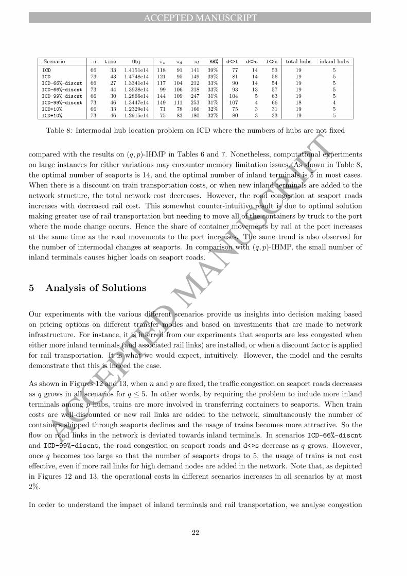
ACCEPTED MANUSCRIPT

ACCEPTED MANUSCRIP

T

Scenario n time Obj πs πd πl RR% d<>l d<>s l<>s total hubs inland hubs

ICD 66 33 1.4151e14 118 91 141 39% 77 14 53 19 5ICD 73 43 1.4748e14 121 95 149 39% 81 14 56 19 5ICD-66%-discnt 66 27 1.3341e14 117 104 212 33% 90 14 54 19 5ICD-66%-discnt 73 44 1.3928e14 99 106 218 33% 93 13 57 19 5ICD-99%-discnt 66 30 1.2866e14 144 109 247 31% 104 5 63 19 5ICD-99%-discnt 73 46 1.3447e14 149 111 253 31% 107 4 66 18 4ICD+10% 66 33 1.2329e14 71 78 166 32% 75 3 31 19 5ICD+10% 73 46 1.2915e14 75 83 180 32% 80 3 33 19 5

Table 8: Intermodal hub location problem on ICD where the numbers of hubs are not fixed

compared with the results on (q, p)-IHMP in Tables 6 and 7. Nonetheless, computational experiments

on large instances for either variations may encounter memory limitation issues. As shown in Table 8,

the optimal number of seaports is 14, and the optimal number of inland terminals is 5 in most cases.

When there is a discount on train transportation costs, or when new inland terminals are added to the

network structure, the total network cost decreases. However, the road congestion at seaport roads

increases with decreased rail cost. This somewhat counter-intuitive result is due to optimal solution

making greater use of rail transportation but needing to move all of the containers by truck to the port

where the mode change occurs. Hence the share of container movements by rail at the port increases

at the same time as the road movements to the port increases. The same trend is also observed for

the number of intermodal changes at seaports. In comparison with (q, p)-IHMP, the small number of

inland terminals causes higher loads on seaport roads.

5 Analysis of Solutions

Our experiments with the various different scenarios provide us insights into decision making based

on pricing options on different transfer modes and based on investments that are made to network

infrastructure. For instance, it is inferred from our experiments that seaports are less congested when

either more inland terminals (and associated rail links) are installed, or when a discount factor is applied

for rail transportation. It is what we would expect, intuitively. However, the model and the results

demonstrate that this is indeed the case.

As shown in Figures 12 and 13, when n and p are fixed, the traffic congestion on seaport roads decreases

as q grows in all scenarios for q ≤ 5. In other words, by requiring the problem to include more inland

terminals among p hubs, trains are more involved in transferring containers to seaports. When train

costs are well-discounted or new rail links are added to the network, simultaneously the number of

containers shipped through seaports declines and the usage of trains becomes more attractive. So the

flow on road links in the network is deviated towards inland terminals. In scenarios ICD-66%-discnt

and ICD-99%-discnt, the road congestion on seaport roads and d<>s decrease as q grows. However,

once q becomes too large so that the number of seaports drops to 5, the usage of trains is not cost

effective, even if more rail links for high demand nodes are added in the network. Note that, as depicted

in Figures 12 and 13, the operational costs in different scenarios increases in all scenarios by at most

2%.

In order to understand the impact of inland terminals and rail transportation, we analyse congestion

22

ACCEPTED MANUSCRIPT

ACCEPTED MANUSCRIP

T

20%

30%

40%

50%

60%

1 2 3 4 5 6 7 8

ICD ICD-99%-dscnt ICD-66%-dscnt ICD10xtra

(a) Road usage percentage

40

52

64

76

88

100

112

1 2 3 4 5 6 7 8

x 10

0000

ICD ICD-99%-dscnt ICD10xtra ICD-66%dscnt

(b) Road Load

110

120

130

140

150

160

170

2 3 4 5 6 7 8

Trill

ions

ICD ICD-99%-dscnt ICD+10% ICD-66%-dscnt

(c) Total costs

Figure 12: Comparison of road and rail usage at seaports as q increases for n = 66 and p = 15

20%

30%

40%

50%

60%

0 1 2 3 4 5

ICD ICD-99%-dscnt ICD-66%-dscnt ICD10xtra

(a) Road usage percentage

6.3E+06

7.5E+06

8.7E+06

9.9E+06

1.1E+07

0 1 2 3 4 5q

ICD ICD-99%-dscnt ICD-66%dscnt

(b) Road Load

1.2E+14

1.3E+14

1.4E+14

1.5E+14

1.6E+14

0 1 2 3 4 5

ICD ICD-99%-dscnt ICD-66%-dscnt

(c) Total costs

Figure 13: Comparison of road and rail usage at seaports as q increases for n = 73 and p = 14

and also, costs for the case when the total number of hubs p and the minimum number of inland

terminals, q, are incremented together. This way, we can observe the impact when the problem itself is

not forced to sacrifice a seaport for an inland terminal. Hence, we can observe the impact of adding an

inland terminal to the set of hubs. As shown in Figures 14 and 15, the proportion of road congestion at

seaport links is considerably decreased and the total operational and fixed costs decreases by at most

5%. Figures 14-18 indicate that the number of containers transferred by trucks to seaports for transfer

through sea links is considerably decreased. There is an increase in road transfer to seaports (mostly

for l<>d) in most scenarios when the number of inland terminals reaches to 2 because there is a better

opportunity to substitute road transfer by rail transfer in a few islands, but the proportion of road

usage remains declining as q grows. Besides installing more inland terminals, the facilities of rail usage

(by new rail links, or discounted rails) promotes the ratio of the rail usage to the road usage. As shown

in Figures 16 and 17, there is a shift in the number of containers shipped to seaports by road to rail as

q grows. Furthermore, the total operations of modal interchange at seaports is significantly deviated

from seaports as shown in Figure 18.

In the following, we compare the fixed costs and congestion costs in seaports. The congestion cost

is associated with the opportunity cost of delays on roads. It is proportional to the number of road

users and reciprocal of the average speed on roads when the capacity of roads is fixed. Since container

transport by trucks increases the number of road users and decreases the average speed, we expect

that the deviation of container transport to rail improves the congestion cost. There are many sophis-

ticated models to incorporate variable traffic flow, network flow equilibrium conditions, and speed-flow

23

ACCEPTED MANUSCRIPT

ACCEPTED MANUSCRIP

T

20%

30%

40%

50%

60%

0 1 2 3 4 5 6 7 8

ICD ICD-99%-dscnt ICD+10% ICD-66%-dscnt

(a) Road usage percentage

45

65

85

105

125

145

0 1 2 3 4 5 6 7 8

x 10

0000

ICD ICD-99%-dscnt ICD+10% ICD-66%-dscnt

(b) Road load

1.1E+14

1.2E+14

1.3E+14

1.4E+14

1.5E+14

1.6E+14

0 1 2 3 4 5 6 7 8

ICD ICD-99%-dscnt ICD+10% ICD-66%-dscnt

(c) Total costs

Figure 14: Comparison of road and rail usage at seaports as q increases for n = 66 and p− q = 9

20%

40%

60%

0 1 2 3 4 5

ICD ICD-99%-dscnt ICD+10% ICD-66%-dscnt

(a) Road usage percentage

5.00E+06

6.00E+06

7.00E+06

8.00E+06

9.00E+06

1.00E+07

1.10E+07

1.20E+07

1.30E+07

0 1 2 3 4 5

ICD ICD-99%-dscnt ICD+10% ICD-66%-dscnt

(b) Road load

1.2E+14

1.3E+14

1.4E+14

1.5E+14

1.6E+14

0 1 2 3 4 5

ICD ICD-99%-dscnt ICD+10% ICD-66%-dscnt

(c) Total costs

Figure 15: Comparison of road and rail usage at seaports as q increases for n = 73 and p− q = 10

5

8

11

0 1 2 3 4 5

Mill

ions

Truck Train

(a) ICD

5

8

11

14

0 1 2 3 4 5

Mill

ions

Truck Train

(b) ICD-66%-dscnt

5

8

11

14

0 1 2 3 4 5 6 7 8

Mill

ions

Truck Train

(c) ICD+25%

Figure 16: Comparison of road and rail usage at seaports in different scenarios as q increases for n = 66and p− q = 8

relationship to come up with optimum congestion costs (Yang and Huang, 1998; Verhoef, 1999). To

measure the cost of congestion in seaports in our study, we use an economic model for congested roads,

which is simple to interpret and requires few parameters. Evans (1992) proposed congestion costs as

follows:

W = β

(1

1− QCap

− 1

)+

βQ

Cap× 1

(1− QCap)2

,

24

ACCEPTED MANUSCRIPT

ACCEPTED MANUSCRIP

T

0.00E+00

3.00E+06

6.00E+06

9.00E+06

1.20E+07

1.50E+07

1.80E+07

0 1 2 3 4 5

Truck Train

(a) ICD

0.00E+00

3.00E+06

6.00E+06

9.00E+06

1.20E+07

1.50E+07

1.80E+07

2.10E+07

2.40E+07

0 1 2 3 4 5

Truck Train

(b) ICD-66%-dscnt

Figure 17: Comparison of road and rail usage at seaports in different scenarios as q increases for n = 73and p− q = 10

where β is a parameter that reflects the monetary value of the equation, and Q and Cap are the total

number of containers using roads and the overall capacity of the road system, respectively. We also

associate cost factors Crr and Crs for the number of containers which change transfer modes between

road and rail (denote it by Xrr), and road to ship (denoted by Xrs), respectively, in order to measure

avoidable usage of seaport infrastructures by using inland terminals. All together, we use the congestion

cost function W +CrrXrr+CrsXrs. Since queues at seaport facilities are not desired, we set Crs � CrrAs shown in Figure 19, with larger number of inland terminals, the total cost of congestion and fixed

costs is minimum for q = 4. In other words, when the intermodal hub location problem parameters

are set to have at least 4 inland terminals, the cost of installations and road congestion at large cities

(in other words, seaports), is minimum. In this way the modelling can give some guidance as to the

level of investment in rail infrastructure that can be justified by the reduction in congestion, though

the practical difficulty is that the congestion costs are carried by all road users, while the infrastructure

has to be paid for by the state or transport companies.

0

20

40

60

80

100

120

140

160

0 5 0 5 0 5

ICD ICD10xtra ICD3

x 10

0000

d<>l d<>s l<>s

ICD + 10% ICD - 66%

q:

(a) n = 66 and p− q = 8

0

20

40

60

80

100

120

140

160

180

0 5 0 5 0 5

ICD ICD10xtra ICD3

x 10

0000

d<>l d<>s l<>s

ICD + 10% ICD - 66%

q:

(b) n = 73 and p− q = 10

Figure 18: Comparison of interchanges at seaports for q = 0, 5

25

ACCEPTED MANUSCRIPT

ACCEPTED MANUSCRIP

T0

50

100

150

200

250

300

350

400

0 1 2 3 4 5

x 10

0000

000

Fixed Costs (inland terminals) Congstion Costs Total Costs

(a) n = 66

0

50

100

150

200

250

300

350

400

0 1 2 3 4 5

x 10

0000

000

Fixed Costs (inland terminals) Congestion Costs Total Costs

(b) n = 73

Figure 19: Trend of congestion costs and fixed costs for new inland hubs

6 Conclusions

In this paper, we present a network design framework as an extension of the traditional hub location

problem. Here, a few important restrictions of the traditional hub location problem are relaxed in order

to model the intermodal network design problem for container transportation. We relax the assumption

that the network is complete. We assume that the cost of interchanges between modes is non-trivial.

The (q, p)-IHMP presented and formulated in this paper is such a network design problem. It includes

3 transport modes and 2 types of hubs. Network flow costs and fixed costs are also incorporated.

We then proved that (q, p)-IHMP is equivalent to the traditional hub location problem in terms of

computational complexity. Furthermore, a dataset based on a real-world problem for intermodal hub

location problems is provided. This includes a sparse network structure, 3 types of links, 2 types of

hubs, cost factors, and flow demands.

An analysis on our computational results on (q, p)-IHMP provides an insight into some of the most

influential factors for decision making in this case study. It is shown that by investing in the estab-

lishment of inland container hubs, the total congestion cost and fixed cost is reduced. Furthermore,

it is shown that the introduction of discounted pricing on rail transportation can influence network

flow, throughput and can lead to congestion reduction at roads around seaports. Through these capital

investment instruments, a larger volume of containers are transferred to seaports through the rail net-

work. This causes shorter queues at ports for loading ships, and a better utilisation of port facilities.

However, not all seaports automatically see reduced congestion due to increased rail facilities, as the

rail station can attract additional truck traffic to transfer containers to rail. Hence careful analysis

using the type of hub location models proposed here is required. In general, a better pricing policy

results in a more efficient usage of port facilities at seaports, and also causes far less road congestion

at the corresponding cities.

The intermodal hub location problem is an important extension of the general hub location problem.

Also, the sparsity of the underlying network reflects a more practical framework for further research.

There is room to extend the intermodal hub location problem to other interesting variations. A varia-

26

ACCEPTED MANUSCRIPT

ACCEPTED MANUSCRIP

T

tion of the problem that considers specific allocation strategies and capacities on arcs and nodes will be

particularly interesting and practically relevant. In addition, the ICD dataset provided in this paper

can be used in the literature of intermodal hub location problems (and hub location problems, in gen-

eral) to design more complex and interesting problems. The new problem also creates a new challenge

as solving the full sized instance, or even medium to large sized instances in the ICD dataset is beyond

the capability of standard integer linear programming solvers (in a reasonably short time) using the

formulation presented here. We are confident that several alternative and more sophisticated mathe-

matical models are possible for the problem that we have presented. We also believe that it is possible

to develop a more tailored, powerful and specialised solution method (or methods) for the problem that

we presented. Indeed, given the potential practical importance of the model, further research is needed

to develop such methods for this problem. The current literature on solutions to hub location problems

suggests that decomposition methods and/or heuristic methods could well be employed as promising

directions. Furthermore, different transfer modes and types of hubs can be exploited for interesting

experimentations and solution analyses with the aim of advising strategic investment decisions and

tactical flow management arrangements. We also believe that future approaches should incorporate

more sophisticated congestion models.

References

I. Akgun and B. Tansel. p-hub median problem for non-complete networks. Comput Oper Res, 95:56–72, 2018.S. Alumur and B. Y. Kara. Network hub location problems: The state of the art. Eur J Oper Res, 190(1):1–21, 2008.S. A. Alumur, B. Y. Kara, and O. E. Karasan. Multimodal hub location and hub network design. Omega, 40(6):927–939,

2012.P. Arnold, D. Peeters, and I. Thomas. Modelling a rail/road intermodal transportation system. Transport Res E-Log, 40

(3):255–270, 2004.T. Aykin. Networking policies for hub-and-spoke systems with application to the air transportation system. Transport

Sci, 29(3):201–221, 1995.J. F. Campbell. Integer programming formulations of discrete hub location problems. Eur J Oper Res, 72(2):387–405,

1994.J. F. Campbell. Hub location and the p-hub median problem. Oper. Res., 44(6):923–935, 1996.J. F. Campbell and M. E. O’Kelly. Twenty-five years of hub location research. Transport Sci, 46(2):153–169, 2012.J. F. Campbell, A. T. Ernst, and M. Krishnamoorthy. Hub location problems. Facility location: applications and theory,

1:373–407, 2002.J. F. Campbell. Hub location for time definite transportation. Comput Oper Res, 36(12):3107–3116, 2009.S. Cetiner, C. Sepil, and H. Sural. Hubbing and routing in postal delivery systems. Ann Oper Res, 181(1):109–124, 2010.O. Dukkanci and B. Y. Kara. Routing and scheduling decisions in the hierarchical hub location problem. Comput Oper

Res, 85:45–57, 2017.A. T. Ernst and M. Krishnamoorthy. Efficient algorithms for the uncapacitated single allocation p-hub median problem.

Location science, 4(3):139–154, 1996.A. T. Ernst and M. Krishnamoorthy. An exact solution approach based on shortest-paths for p-hub median problems.

INFORMS J. Comput., 10(2):149–162, 1998a.A. T. Ernst and M. Krishnamoorthy. Exact and heuristic algorithms for the uncapacitated multiple allocation p-hub

median problem. Eur J Oper Res, 104(1):100–112, 1998b.A. T. Ernst and M. Krishnamoorthy. Solution algorithms for the capacitated single allocation hub location problem. Ann

Oper Res, 86:141–159, 1999.A. T. Ernst, H. Hamacher, H. Jiang, M. Krishnamoorthy, and G. Woeginger. Uncapacitated single and multiple allocation

p-hub center problems. Comput Oper Res, 36(7):2230–2241, 2009. doi: 10.1016/j.cor.2008.08.021.A. W. Evans. Road congestion pricing: when is it a good policy? Journal of transport economics and policy, pages

213–243, 1992.R. Z. Farahani, M. Hekmatfar, A. B. Arabani, and E. Nikbakhsh. Hub location problems: A review of models, classification,

solution techniques, and applications. Computers and Industrial Engineering, 64(4):1096–1109, 2013.S. Gelareh, S. Nickel, and D. Pisinger. Liner shipping hub network design in a competitive environment. Transport Res

E-Log, 46(6):991–1004, 2010.

27

ACCEPTED MANUSCRIPT

ACCEPTED MANUSCRIP

T

M. Ghane-Ezabadi and H. A. Vergara. Decomposition approach for integrated intermodal logistics network design.Transport Res E-Log, 89:53–69, 2016.

R. Ishfaq. LTL logistics networks with differentiated services. Comput Oper Res, 39(11):2867–2879, 2012.R. Ishfaq and C. R. Sox. Intermodal logistics: The interplay of financial, operational and service issues. Transport Res

E-Log, 46(6):926–949, 2010.R. Ishfaq and C. R. Sox. Hub location–allocation in intermodal logistic networks. Eur J Oper Res, 210(2):213–230, 2011.P. Jaillet, G. Song, and G. Yu. Airline network design and hub location problems. Location science, 4(3):195–212, 1996.Z. Kartal, S. Hasgul, and A. T. Ernst. Single allocation p-hub median location and routing problem with simultaneous

pick-up and delivery. Transport Res E-Log, 108:141–159, 2017.J. G. Klincewicz. Hub location in backbone/tributary network design: a review. Location Science, 6(1):307–335, 1998.M. Labbe and H. Yaman. Solving the hub location problem in a star–star network. Networks, 51(1):19–33, 2008.S. Limbourg and B. Jourquin. Optimal rail-road container terminal locations on the european network. Transport Res

E-Log, 45(4):551–563, 2009.R. F. Love, J. G. Morris, and G. O. Wesolowsky. Facilities location. 1988.H. Mokhtar, M. Krishnamoorthy, and A. T. Ernst. The 2-allocation p-hub median problem and a modified Benders

decomposition method for solving hub location problems. Submitted, a.H. Mokhtar, M. Krishnamoorthy, and A. T. Ernst. A modified Benders method for the single and multiple allocation

p-hub median problem. (to appear), b.H. Mokhtar, M. Krishnamoorthy, and A. T. Ernst. A new Benders decomposition acceleration procedure for large scale

multiple allocation hub location problems. (to appear), c.M. E. O’Kelly. The location of interacting hub facilities. Transport Sci, 20(2):92–106, 1986.M. E. O’Kelly. A quadratic integer program for the location of interacting hub facilities. Eur J Oper Res, 32(3):393–404,

1987.W. B. Powell and Y. Sheffi. The load planning problem of motor carriers: Problem description and a proposed solution

approach. Transportation Research Part A: General, 17(6):471–480, 1983.A. E. Prasetyo and F. Hadi. Analisis pemindahan moda angkutan barang di jalan raya pantura pulau jawa (studi kasus:

Koridor surabaya-jakarta). Jurnal Teknik ITS, 2(1):E17–E22, 2013.G. Sen, M. Krishnamoorthy, N. Rangaraj, and V. Narayanan. Exact approaches for static data segment allocation problem

in an information network. Comput. Oper. Res., 62:282–295, 2015.G. Sen, M. Krishnamoorthy, N. Rangaraj, and V. Narayanan. Mathematical models and empirical analysis of a simulated

annealing approach for two variants of the static data segment allocation problem. Networks, 68(1):4–22, 2016.P. Z. Tan and B. Y. Kara. A hub covering model for cargo delivery systems. Networks, 49(1):28–39, 2007.E. T. Verhoef. Time, speeds, flows and densities in static models of road traffic congestion and congestion pricing. Regional

Science and Urban Economics, 29(3):341–369, 1999.H. Yang and H.-J. Huang. Principle of marginal-cost pricing: how does it work in a general road network? Transportation

Research Part A: Policy and Practice, 32(1):45–54, 1998.

28