An interactive simulation program for visualizing complex...

Computer Physics Communications 124 (2000) 60–75www.elsevier.nl/locate/cpc

An interactive simulation program for visualizing complexphenomena in solids

J. Merimaa, L.F. Perondi∗,1, K. KaskiLaboratory of Computational Engineering, Helsinki University of Technology, P.O. Box 9400, FIN-02015 HUT, Finland

Received 16 February 1999; received in revised form 2 June 1999

Abstract

In the present article an interactive simulation program illustrating grain boundary and fracture phenomena in solids isdescribed. The dynamical behaviour of a two-dimensional Lennard-Jones model system under stress, with either a grainboundary or an initial crack, is simulated through a molecular dynamics algorithm. All parameters defining the system andthe dynamical load are set through a graphical user interface. A run-time representation of the system is displayed on a graphicswindow, which has been endowed with magnification and other visualization aid tools. The program runs on a UNIX-X11Window System platform. The graphical part relies on the MOTIF library. The program has been devised for illustrativepurposes. It displays the main elements of an interactive simulation and may be regarded as giving an illustration of the conceptof interactivity. Due to the power of run-time animations in conveying ideas and concepts, it may prove to be useful, as well, asan instructional tool. 2000 Elsevier Science B.V. All rights reserved.

PACS:07.05.T; 79.20.A; 01.50.H; 62.20MKeywords:Computer modeling and simulation; Grain boundaries; Fracture; Dislocations; Molecular dynamics; Graphical interface

PROGRAM SUMMARY

Title of program: Fracture

Catalogue identifier:ADKS

Program Summary URL:http://www.cpc.cs.qub.ac.uk/cpc/summaries/ADKS

Program obtainable from:CPC Program Library, Queen’s Univer-sity of Belfast, N. Ireland

Computer for which the program is designed and others on which itis operable:

∗ Corresponding author; e-mail: [email protected] Permanent address: Instituto Nacional de Pesquisas Espaciais –

INPE, P.O. Box 515, 12-227-010 São José dos Campos SP, Brazil.

Computers:DEC ALPHA 300 and equivalent or superior machines

Installations: Lab. of Computational Engineering, Helsinki Univer-sity of Technology, Helsinki, Finland

Operating systems under which the program has been tested:UNIX

Programming language used:C with MOTIF and standard libraries

Memory required to execute with typical data:Minimum of2 Mbytes but depends on system size

No. of bytes in distributed program, including test data, etc.:37 629bytes

Distribution format: uuencoded compressed tar file

0010-4655/00/$ – see front matter 2000 Elsevier Science B.V. All rights reserved.PII: S0010-4655(99)00264-7

J. Merimaa et al. / Computer Physics Communications 124 (2000) 60–75 61

Keywords: Lennard-Jones, molecular dynamics, fracture, crack,dislocations

Nature of physical problemIn a typical research activity involving simulations of complex phys-ical systems, one is often faced with a ‘research loop’, which maybe loosely described as follows: definition of input data; runningof a simulation, outputting data to a storage disk; post-processingof the accumulated data for extracting relevant information withthe eventual aid of graphics and numerical packages; definition ofnew input parameters and, closing the loop, starting a new simu-lation run. Advances in computer hardware, mainly faster proces-sors, and the increased availability of software development tools,with plenty of graphics resources, have been markedly increas-ing the feasibility of alternative solutions for improving the abovescheme.

Method of solutionInteractive simulations offer an attractive option for the study of sys-tems in which a great deal of feedback, in the sense described above,is required. They are also ideal for teaching purposes. The presentprogram gives an illustration of an interactive simulation environ-ment. The dynamical behaviour of a two-dimensional Lennard-Jones ‘solid’ under stress, with either a grain boundary or an initialcrack, is simulated through a molecular dynamics algorithm.

Restrictions on the complexity of the problemThe interactiveness concept strongly relies on the display of ananimated graphical representation of the system. The quality of theanimation depends on the rate with which frames are displayedon the graphical display window. This rate, in its turn, dependson the iteration time of the simulation algorithm. Hence, the sizeof the systems which may be investigated, while maintaining anacceptable animation quality, depends on the machine processor.Systems with up to 50 000 atoms give fair animations for thetarget machine given above. Subjecting the system to strain ratessufficiently high for inducing atomic displacements of the order ofthe mean inter-atomic distance in one integration step will causethe program to collapse. Studies at such high rates will requiremodifications of the MD algorithm. The implementation of anadaptive integration method will, most possibly, be enough for mostapplications.

Typical running timeThe typical running time is machine and system size dependent.

Unusual features of the programAlthough the program has been originally designed for illustrativepurposes, its final version incorporates features which, we believe,render it in a good standard for research work in two-dimensionalmodels, provided a better treatment is given to thermal effects. Inparticular, it has been endowed with a control button which allowsthe user to generate an instantaneous ‘snapshot’ of the graphicsscreen. The image is stored in a bitmap file (X11 standard), createdunder the same directory in which the program is running.

LONG WRITE-UP

1. Introduction

The application of computers and computationaltechniques to the study of physical phenomena isby now a well-established and important branch ofmodern science. The course of its development hasclosely followed the improvement on the availabil-ity of hardware and software resources. In the wakeof these developments, applications evolved, in ma-terials research, for example, from the numerical so-lution of small scale systems of algebraic equationsto the currentmulti-million atomsmolecular dynam-ics (MD) simulations of various phenomena in liq-uids and solids [1–3]. The current availability of com-puter resources, with desktop machines exhibiting theperformance of the supercomputers of yesterday, hasbeen stimulating new developments at an impressiverate [4]. Confining ourselves to examples directly re-lated to the subject of this article, we quote the de-velopment of interactive simulations of many-particlesystems [5] and of specially-tailored techniques andtools for the analysis of data arising from the simula-tion of complex physical phenomena [6,7].

Conceptually, interactive simulations may be envis-aged as the association of visualization tools with anumerical simulation code in a message-oriented orevent-driven environment. They present very distinc-tive advantages when compared toconventionalsimu-lations. In the latter, the way simulation data are gener-ated and analyzed may schematically be described asfollows: define initial parameters, run the simulationand output the data to a storage medium and in a post-processing phase analyze the results with the even-tual aid of numerical and graphics packages; eventu-ally, define a new set of initial parameters and performa new run. In an interactive simulation environment,otherwise, the simulation data may be output directlyto a graphics environment and simulation parametersmay be changed at any time. In a many-particle sys-tem, for instance, it is then possible to visually accom-pany the time evolution of the system and to imposechanges to it at run-time by assigning new values toimportant parameters. This ability to drive the systeminto new states, guided by a visual feedback, createsa rich research environment, which offers several pos-

62 J. Merimaa et al. / Computer Physics Communications 124 (2000) 60–75

sibilities, ranging from a sensitivity analysis of rele-vant parameters to the emulation of situations that maygive valuable insight into phenomena of great com-plexity.

Simulations aimed at the study of the mechanicalproperties of solids, for the richness of the phenom-ena they exhibit, are natural candidates for being en-dowed with an interactive interface. In the present ar-ticle we illustrate some of the potentialities of an in-teractive simulation environment by considering phe-nomena associated to fracture and grain boundary insolids. More specifically, we will describe a programspecially designed for illustrating such phenomenaand give a concise guide about its use. Despite the sim-plicity of the implemented model – a two-dimensionalLennard-Jones solid – it has proved to be rich enoughto illustrate important phenomena such as emissionand propagation of dislocations, ductile and brittlefracture behaviour and grain boundary relaxation.

The program has been developed as part of an effortto assess the relevance of the interactive approachto molecular dynamics simulations of solid statephenomena. Despite this background, the presentationgiven here is centred on a description of the developedprogram and its use, rather than on a descriptionand analysis of the interactive approach itself. Onlythose aspects of interactivity which are relevant to anunderstanding of the program have been consideredin some detail. The program has been devised forillustrative purposes. It displays the main elementspresent in an interactive simulation and is intendedto give an illustration of the value of interactivity incomputer simulations. Owing to the physical modelimplemented and the help animation may give in theexplanation of physical phenomena, it may prove tobe useful, as well, as an instructional tool in materialsscience and solid-state physics courses.

The article is organized as follows. In Section 2 wegive the main definitions and some physical motiva-tions related to the study of grain boundaries and frac-ture in solids. Main technical aspects relative to theimplemented algorithm are also addressed. Section 3is dedicated to a general description of the program,its structure and the graphical interface. Some exam-ples are described in Section 4. Final comments andconclusions are given in Section 5.

2. Model

In this section we address some conceptual aspectsrelative to the program. The exposition is dividedin two parts. Firstly, we give a brief introductionto physical concepts related to grain boundaries andfracture in solids. Only very general aspects, which arerelated to the implemented model and the examplesin Section 4, are contemplated. Detailed informationmay be found in the references. Since we will bedealing with a two-dimensional model we emphasizethe role of dimensionality. Secondly, an overview ofthe simulation model and a description of the mainvisualization tools are given in Sections 2.2 and 2.3,respectively.

2.1. Fracture and grain boundaries

The subjects of fracture and interfaces in solids, to-gether with their associated phenomena, are currentlyamong the central research themes in materials sci-ence.

Single-phase interfaces, such as those present inpolycrystalline materials, are generally referred to asgrain boundaries [8]. Understanding the structure andthe dynamics of grain boundaries and their interactionwith defects is one of the major challenges in settingup realistic models for the mechanical behaviour ofmaterials. While in three dimensions there are five de-grees of freedom in the formation of a boundary be-tween two crystallites, in two dimensions (2D) thereare only two. In this latter case, for equal crystallites,it suffices to define the rotation of each crystallite withrespect to the interface line to characterize any possi-ble boundary. Such boundaries are termed tilt bound-aries. In three dimensions (3D), a tilt boundary, par-alleling the 2D case, may be thought as formed bythe rotation of two initially equally oriented crystal-lites through a common rotation axis. Tilt boundariesmay be classified into symmetric or asymmetric, de-pending upon whether each crystallite is or is not themirror image of the other.

The imperfections at a low angle 3D tilt grainboundary may be interpreted asedge dislocations[9].A perfect edge dislocation is a line defect associatedwith the abrupt end of a plane of atoms inside the bulkregion of an otherwise perfect crystal. The dislocationline is given by the faulty edge of this plane. Simi-


larly, imperfections at a 2D grain boundary may be re-garded as the 2D equivalent of an edge dislocation. Incomplete analogy with the 3D case, 2D edge disloca-tions are formed by the abrupt end of a line of atoms inthe internal part of a 2D layer of atoms. The 2D edgedislocation is the defect associated with the tip of thefaulty line. Appendix 5 gives further details about 2Ddislocations in a triangular lattice. Great interest existsin the microscopic structure of grain boundaries. It de-pends on geometric parameters, such as the orientationof the crystallites, as well as on the interatomic poten-tial. Studies of grain boundary structure are generallycarried out by initially generating the boundary in ac-cordance with the geometrical constraints and then let-ting the resulting system to relax.

The understanding of fracture phenomena is ofgreat relevance from both the scientific and techno-logical points of view [10]. The literature on the sub-ject is quite extensive [11]. We will limit ourselves toa brief description of the main facts about fracture incrystalline materials. The way a macroscopic fracturesprings up and evolves in a strained sample is stronglydependent on thebrittlenessof the solid. In very brit-tle materials a crack with a sharp tip propagates at veryhigh speeds, leading invariably to cleavage of the sam-ple. The crack path may show irregularities, the originof which has been the subject of some debate [12,13].At the other extreme, in ductile materials, a crack maynot propagate at all. Up to comparatively high strainlevels, there is only the emission of dislocations, thenet effect of which is to causeblunting of the cracktip. Most of the current research focus on the mod-eling of the ductile/brittle behaviour of the crack tipin terms of a microscopic, atomistic level, model po-tential. Two-dimensional models have attracted a greatdeal of attention [2,3,14–16].

The program, object of this article, allows thedefinition of a two-dimensional system containingeither a grain boundary or an initial crack (or both).Both symmetric and asymmetric tilt boundaries maybe generated. The implemented resources permit thesimulation of grain boundary relaxation and the studyof the effect of stress and temperature on it. Thefracture-related implementation permits the placing ofan initial crack, with chosen rectangular dimensions,anywhere in the simulation area. The main objective isto follow what happens to the resulting structure whenit is subjected to strain at a given temperature. To this

effect, the user may specify at run-time a given strainlevel and the rate at which it is applied. Also, makinguse of run-time controls, the user may set, at anymoment, a new temperature value. The program alsofeatures controls which allow the study of the effectof changes in the inter-atomic potential on the thegrain boundary and fracture phenomena. Next we givedetails of the simulation and visualization algorithms.

2.2. Simulation model

Inter-atomic interactions have been modelled by aLennard-Jones pair potential

U(r)= e((

σ

r

)12

−(σ

r

)6), (1)

where r is the inter-atomic distance,σ defines theequilibrium distancere through the expressionre =21/6σ and e fixes the value of the potential at theequilibrium distance. Owing to the symmetry of thepotential the equilibrium atomic arrangement is atriangular lattice. A conventional molecular dynamics(MD) algorithm has been implemented [17,18]. Inorder to speed up the computations the interactionrange has been limited in the usual way, by settingthe potential to zero beyond a maximum inter-atomicdistancer = rc. To avoid an anomalous behaviourof the force atr = rc, a linear term with the form(r − rc) dUdr |r=rc has been subtracted fromU . Forreasonable values ofrc this approximation has theminor side effect of slightly changing the equilibriumdistance. The user may adjust the values ofe and rcin order to endow the model with a brittle or ductilecharacter. Generally, large values ofe and small valuesof rc favour a brittle behaviour.

The simulations are carried out in the micro-canon-ical ensemble. Temperature is equated to kinetic en-ergy, even when the system is far from thermo-dynamical equilibrium. In each run the system startswith a given instantaneous value of the kinetic energy,which is fed in by assigning an initial velocity to eachparticle. The velocity vectors have equal magnitudeand are given a random orientation. The excess kineticenergy in any of the directions is then removed. Theuser may change at any moment the energy contentof the system by specifying a new instantaneous valuefor the kinetic energy. Arrow buttons are provided for


this purpose. The new value is enforced by simultane-ously re-scaling the magnitude of the velocity vectorsof all particles. Alternatively, the temperature duringa whole simulation run may be kept below a certainvalue (the default value is 20 K) by checking a boxcontrol specially set for this purpose. The operativemechanism triggered by this control is equivalent to acontinual pressing of the down temperature arrow but-ton when the temperature exceeds the threshold valuein effect. These features have been implemented withthe purpose of controlling the total energy in the sys-tem, which can substantially increase when the sys-tem is strained. We emphasize that this scheme gives apoor representation of thermal effects. A proper treat-ment would involve the use of some intrinsic mecha-nism for emulating the heat exchange with an externalheat reservoir [18].

When attempting to study the dynamics of bulk phe-nomena through simulations in a finite system, even-tual boundary effects have to be taken into account. Inthe present simulations, reflection of strain waves atthe boundaries are the main visible effect. Reflectedwaves may have a noticeable influence on the waycracks evolve, mainly due to interference. They mayalso significantly affect the way relaxation takes placeat grain boundaries. No special features have been in-corporated in order to minimize such effects. Addi-tionally, since no intrinsic dissipative mechanism hasbeen implemented wave coherency is longer lived,giving enhanced interference effects. The only avail-able way for limiting the influence of such effects isto control the total energy content of the system in themanner discussed above.

Strain is applied to the system by changing itsx-dimension (parallel to the screen bottom edge)by an amount and at a rate specified by the user.Practically, this is accomplished by rigidly moving,at a constant velocity, the atoms belonging to a fewcolumns of the external vertical (y-direction) bordersof the simulation area. In order to avoid undesirededgereconstructions, the atoms in these ‘fixed’ borders arenot allowed to move in thex-direction as a resultof interactions. Their movement in they-direction,however, is completely unconstrained. The user maychoose the width of the fixed borders. Thefixed borderfeature may be switched on/off at any moment. Freeboundaries are important, for instance, when studyingrelaxation at grain boundaries.

2.3. Feature highlighting

Extracting the desired information from a batch ofdata is an important aspect when setting up an inter-active simulation. Interesting phenomena are usuallyhiddenin the data and a feature extraction algorithmhas the objective of searching for and isolating theirdata structure for subsequent processing.

In the present case, the most direct way of display-ing system features is to show a graphical represen-tation of the atoms on the screen. This is, in fact, themain graphical output of the code at hand. Visualiza-tion of phenomena may be enhanced by secondarytools, which operate directly on the graphics screen.Independent transverse and longitudinal (x- and y-directions, respectively) magnification (zooming) toolsare examples. Their implementation is quite straight-forward and they proved to be ideal for visualizing linedefects. By a careful tuning of the magnification fac-tor they may also greatly improve the visualization ofextended phenomena, such as strain waves. Further in-sight into the complexities of the exhibited phenomenamay be achieved by arranging the particles into groupsaccording to some criterion and then differently repre-senting each group on the screen. A common schemeis to assign different colours to different groups. Thecode includes one such feature. The atoms are strati-fied into categories according to the value of their ki-netic energy. A relative scale, in which the averagekinetic energy is set to the midpoint, is used for thispurpose. Particles are then displayed on the screen ac-cording to a colour scheme which associates light redto the most energetic particles and black to the leastenergetic ones. The intermediate cases are shown withdifferent shades of red. Such scheme enhances the vis-ibility of phenomena taking place near boundaries anddefects.

In addition to the particle representation discussedabove, afield representationhas also been imple-mented. The user may switch between the two repre-sentations at any moment. In the latter representationthe velocity field at different length scales is displayed.The length scale may be continuously changed fromthe microscopicto themacroscopic(i.e., comparableto the size of the system) limits. In themicroscopiclimit, an arrow in the direction of the velocity of aparticle is drawn directly at the particle position. Thisgives a clear view of the dynamical behaviour of the


microscopic velocity field. The representation at largerscales is constructed through an averaging process: thesimulation area is covered with a grid having a latticeparameter size specified by the user; an average posi-tion and velocity is then computed for each grid squareby averaging over the particles which are within itsborders; finally, at each of the computed average posi-tions an arrow giving the direction of the average ve-locity is drawn on the screen. The final picture is alarger scale representation of the velocity field.

3. Description of the interface

As already mentioned, the program consists essen-tially of three modules: an MD simulation algorithm,a graphics window for output of data and a user in-terface for input of parameters. In a very schematicdescription, we may say that these modules have beenintegrated in an event-driven environment which han-dles the exchange of information between them, andprocesses any actions requested by the user at run-time. Fig. 1 schematically illustrates the flow of infor-mation.

The program has been written in C and developedfor an X11 Window System platform. All graphicsare based on the MOTIF library. A great deal ofUNIX workstations make use of this platform. A de-tailed description of the programming environmentmay be found in Refs. [19–21]. In this section welimit the discussion to a description of the user inter-face.

Figs. 2 and 3 show the two initial windows whichshow up at startup. The window shown in Fig. 2,labelled ‘Parameters’, allows the user to select the‘fixed’ parameters of the simulation. These are generalparameters which define the main characteristics of

Fig. 1. Schematic structure of an interactive simulation program.The window manager handles the exchange of data among thedifferent modules.

the simulated system, and which are held constantthroughout a simulation run. They are organized intogroups, under a descriptive header. The groups, in theirturn, are aligned into columns. Table 1 gives a generaldescription of each group.

The second window, shown in Fig. 3 and named‘Fracture’, contains, in a broad sense, four categoriesof elements: a text window displaying run-time data;a graphics window giving a run-time graphical rep-resentation of the system; control widgets giving theuser some control on the way data are displayed onthe graphics window and control widgets allowing thechange of simulation parameters at run-time. All ele-ments in this window are described in Table 2.

The program has, essentially, two operating modes:a initialization mode and a running mode. In the ini-tialization mode, the user defines the general charac-teristics of the system to be simulated by setting thecontrols in the window ‘Parameters’. Notice that thegraphics window, in the window ‘Fracture’, is activeeven in this mode and displays an updated representa-tion of the system. The text pane is also active. Whenthe user presses theOK button at the lower right cor-ner, only the window ‘Fracture’ remains open. Press-ing the Run button in this latter window causes theprogram to enter the running mode. In this mode thesimulation algorithm is active and the graphics win-dow is updated at a rate given by theUpdate stepcon-trol widget setting.

The user may suspend/resume the simulation at anymoment by pressing thePause/Runbutton. Whenthe buttonNew is pressed, the program is suspendedand the window ‘Parameters’ is popped up. At thispoint, the user may either select new settings andbegin a new simulation run by pressing theOK buttonor cancel the operation, through theCancel button.The pressing of either buttonpops downthe window‘Parameters’. When the buttonQuit is pressed allwindows are closed and the program ends. Finally,the buttonSnapshotallows the user to dump to afile the current image in the graphics window. Theimage is stored in a file with X11 standard bitmapformat. Consecutive files generated during the samesession are labelled with consecutive letters. The fileshave names with the formatFracture_L.img, whereLstands for any letter of the alphabet, either capital orlower case.


Fig. 2. Window ‘Parameters’. Initialization window with controls for definition of the ‘fixed’ parameters of the simulated system.

Normalization constants have been chosen such thatthe default (initial) settings for the lattice parameter(a = 1) and the potential (e= 1) reproduce a LJ pair-potential appropriate for the study of copper, as givenin Ref. [22]. Distances are given in units of the latticeparameter for copper (a0= 3.60×10−10 m [23]); timehas been normalized to one picosecond (t0= 10−12 s);the integration step is equal to four femtoseconds, i.e.,each MD step corresponds to the elapsing of one suchtime interval; the elapsed time displayed in the mainwindow is given in units of one femtosecond; energiesare given in units ofm0(a0/t0)

2= 1.37736× 10−20 J,wherem0 is the mass of one atom of copper (m0 =1.055206× 10−25 kg [23]). Finally, temperatures aregiven directly in Kelvin units. Table 3 gives a summaryof the main equations and units.

Details about the program files and command lineoptions are given in Appendices 5 and 6.

4. Examples

In this section we describe and comment on somefew illustrative examples. The presentation has twopurposes, namely giving a brief introduction to the useof the program and displaying some of the potentiali-ties of an interactive simulation environment.

4.1. Tilt grain boundary

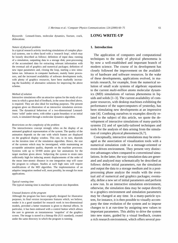
By adjusting the settings according to the valuesgiven in Table 4 under the headingsymmetricandletting the resulting system to relax, a 12◦ symmetrictilt boundary is formed. Please, note that theFix edgescheck box in the Strain pane should be uncheckedin this example. The stable configuration shown inFig. 4 is reached after 21.2 picoseconds (21 200 in thetime display). Note that the defects appearing in theboundary region are 2D dislocations, of the same type


Fig. 3. Window ‘Fracture’. Contains the graphics window, the text pane and the controls which allow the change of parameters at run-time.

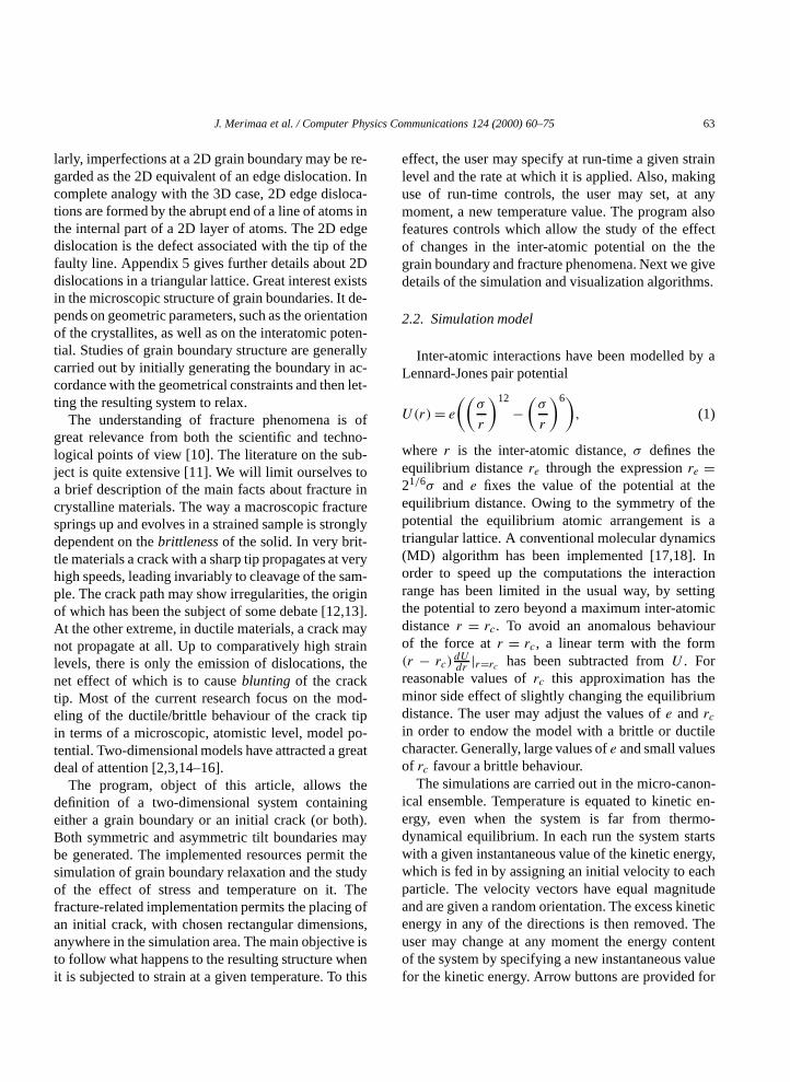
as the ones described in Appendix 5. The observedvertical piling of the dislocations, highlighting theposition of the boundary, may be interpreted as a resultof the interaction between similar dislocations [9].A close look at one of the dislocations may beachieved by settingx = 5 andy = 5 in theView sizepane and setting theAtom diam.scale to 93. If thevisible dislocation is then repositioned at the centre ofthe graphics window, through the sliding bar controls,the obtained image will resemble the one shown inFig. 5.

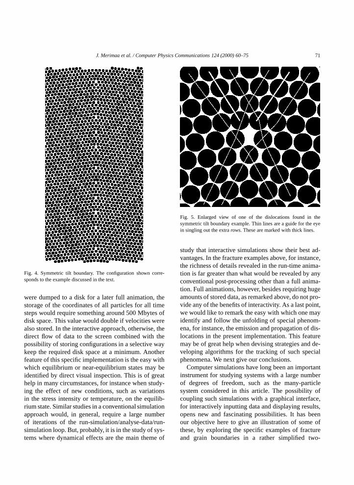
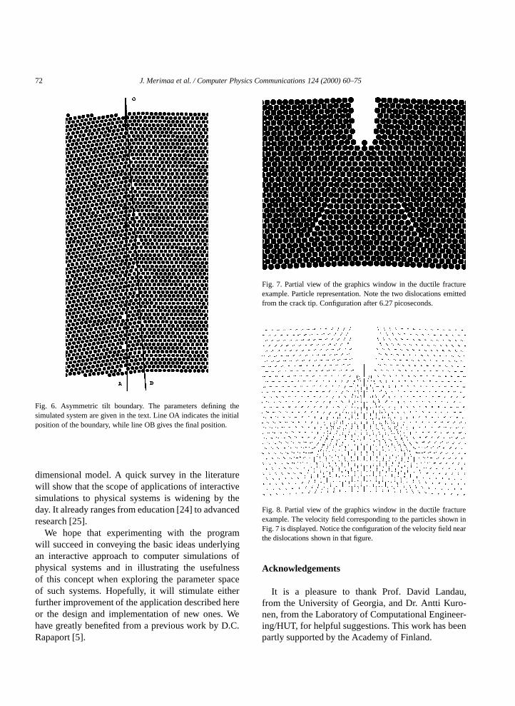
The settings under the headingasymmetricin Ta-ble 4 give an initial configuration for the formationof a 9◦ asymmetric tilt boundary. After about 28.0 pi-coseconds, the structure relaxes to the configurationshown in Fig. 6. Most of the dislocations are now ontop of a line which deviates from the vertical by an

angle around 4.5◦. If we take the aforementioned lineas reference it is easily seen that both crystallites aresymmetrically oriented with respect to it. The finalconfiguration, therefore, is again that of a symmetri-cal tilt boundary. This is an example of grain bound-ary movement. The vacancies seen at the bottom partare due to the non-conservative movement of some ofthe dislocations (see Appendix 5). A close look at thevacancies and dislocations may be achieved with thezoomingsettings given in the previous example.

Grain boundaries tend to become unstable with in-creasing temperature. One may get some insight intothis phenomenon by repeating the above examples andimposing changes to the temperature of the system af-ter the initial equilibrium boundary has been formed.Also, the application of stress, be it compressive ortensile, causes changes in the equilibrium configura-


Table 1Description of the controls in the window ‘Parameters’. The symbols in parenthesis give the unit in which the corresponding control is expressed.Please refer to Table 3 for a definition of the used units

Column 1 – General parameters

Sim. area

x, y initial x- andy-dimensions of simulation area (a0).

Lattice parameter lattice parameter size.

Potential

e minimum value of the LJ pair-potential (Eq. (1)) (u0);

rc cut-off radius of the pair-potential (a0).

Border width defines a stripe at the external longitudinal borders with the specified width, inside which all atoms are constrainedto move only along they-direction; when strain is applied, all atoms inside this stripe are rigidly moved with thespecified strain rate (a0).

Column 2 – Definition of the boundary

Boundary when the box is checked the system is split into two independent sub-lattices, right and left, of equal area. Sinceeach sub-lattice may be rotated independently of the other, boundaries with an arbitrary orientation may beformed.

Rotations

l, r angle of rotation in degrees of the left and right sub-lattices, respectively.

Displacement

x boundary gap as measured from the centre of the closest edge atoms (a0);

y microscopicy-displacement of one sub-lattice with respect to the other (a0).

Column 3 – Crack geometry and positioning

Init. crack checking of the box causes a rectangular crack to be inserted into the system. This is the initial crack for afracture ‘experiment’. The remaining controls in this column define the crack position in the simulation area, itsrectangular dimensions and the angle itsx-edge makes with thex-edge of the simulation area. All distances arein units of (a0).

Crack centre

x, y x- andy-positions of the crack centre (a0).

Crack size

x, y x- andy-lengths of the crack area (a0).

Crack angle angle, in degrees, between thex-edges of crack and simulation area.

tion of the boundary. These changes may be followedby checking theFix edgesbox and setting values forthe total strain and the time duration of its applicationin the corresponding controls. All these controls are inthe Strain pane.

4.2. Brittle versus ductile fracture

Here we briefly consider two examples which illus-trate the limiting cases of brittle and ductile fracture.Table 4, under the headingfracture, gives the settingsfor both cases. In both cases, strain is applied at thevery beginning of the simulation.

In the ductile fracture example, it is observed thatthe crack tip initially advances for a few atomiclayers and then a pair of dislocations is emitted. Afterthis event, the crack tip position remains practicallystationary and undergoes an accentuated blunting asfurther dislocations are emitted. Several processes aretriggered by the dislocation emission. Among them,the heating up of the system and the generation ofstrain waves are particularly noticeable. These effectsmay be better appreciated by repeating theexperimentbut now accompanying the unfolding of events in thevelocity fieldrepresentation (Vectorsbutton). Figs. 7and 8 display the configuration after 6.27 picoseconds


Table 2Main Elements of the window ‘Fracture’. The symbols in parenthesis give the unit in which the corresponding control is expressed. Please referto Table 3 for a definition of the used units

Text window and its elements

Text window displays static and run-time data about the system. The displayed data are:

Step elapsed time (10−3× t0);

Atoms total number of atoms in the system;

Size x- andy-dimensions of the simulation area (a0);

Centre coordinates of the position in the simulation area which is at the centre of the graphics window (a0);

Etot, Ek total energy and kinetic energy per particle, respectively (u0);

Temp temperature in Kelvin degrees.

Graphics window and related elements

Graphics window displays a run-time graphical representation of the system. The sliding bars allow repositioning the simulationarea in the graphics window.

View size pane the two controls in this pane define the scale factors for thex- andy-axis. Their precise meaning are:x- andy-dimensions of the part of the simulation area which is being shown in the graphics window (a0).

Atom diam. control allows the user to change the size of the objects (vectors or circles) displayed in the graphics window;

Vectors box when checked the graphics window display afield representation(see text) of the system;

Averaging control coarse grid size for the vector representation (Section 3) (a0).

Run-time parameters

Strain pane the controls in this pane define the total strain and the strain rate to which the system will be subjected when theApply button is pressed.

Fix edges when checked the external longitudinal borders are fixed (as described in Section 3);

% total strain;

t time interval in which the strain defined in the control above is applied to the system (in femtoseconds)(10−3× t0).

Pressure defines the intensity of a force applied to each particle at the transversal borders (f0).

Temperature allows the user to control the kinetic energy content of the system (as discussed in Section 3).

Table 3Normalization constants and main equations. The variablescut , a and e hold the settings of the corresponding controls in the window‘Parameters’

Main equations: rc = cut a/√

2

σ =(

1

2

(1− (1/cut)7

1− (1/cut)13

))1/6

a/√

2

d2r

dt2= 110.09e

((σ

r

)13− 1

2

(σ

r

)7−((

σ

rc

)13− 1

2

(σ

rc

)7))

U(r)= 9.17e

((σ

r

)12−(σ

r

)6− 12

r − rcσ

((σ

rc

)13− 1

2

(σ

rc

)7))Units: a0= 3.608× 10−10 m (unit of distance)

t0 = 10−12 s (unit of time)

f0= 3.806× 10−11 N (unit of force)

m0= 1.055× 10−25 kg (unit of mass)

u0= 1.37736× 10−20 J (unit of energy)


Table 4Settings for the examples discussed in the text

Grain boundary Fracture

Symmetric Asymmetric Ductile Brittle

Sim. area x: 80 80 Sim. area x: 60 60

y: 40 45 y: 20 30

Lat. param. 1.0 1.0 Lat. param. 1.0 1.0

Potential e: 1 1 Potential e: 1 20

rc: 2.1 2.1 rc: 2.1 2.1

Rotations l: 6 9 Crack center x: 0 0

r: −6 0 y: 7.5 12.5

Displacements x: 0.5 0.6 Crack size x: 1.0 1.0

y: 0.6 −0.3 y: 5.0 10.0

Crack angle 0 0

Obs.: Obs.:In the grain boundary examples the check boxFix edgesshouldbe unchecked. Convenient settings for theView size pane forthese particular examples arex = 32 andy = 43.

In the first example, appropriate settings for the strain rate are:% 5, t 8000. Corresponding settings for the second case are% 10, t 16000. In both cases, for a close look at the crack tip,convenient settings of theView sizepane arex = 30 andy = 30,with repositioning of the crack at the centre of the graphics area.

in the particle and field representations, respectively.A close view of the events taking place near thecrack tip may be achieved through the magnificationtools described in Section 3 (View sizepane). Forinstance, in the present example, the settings30and 10 for the x- and y-directions, respectively,enhances the visualization of the family ofmostdense linesparallel to thex-direction. With thesesettings and positioning the crack tip at the centreof the display window it is possible to follow ingreat detail the events preceding the emission ofthe pair of dislocations. The enhanced visibility ofdislocations and their movement is one of the specialfeatures of thiszoomingscheme. Toggling between theparticle and vector representations further enhancesthe visibility of the phenomena taking place.

The brittle fractureexperimentis conducted in asimilar way as in the ductile case, except for one im-portant difference – in order to enhance the brittle be-haviour the extra heat generated by thebreakingofbonds must be continually removed. This is accom-plished by checking the boxLow temperature. Con-trary to the ductile case, the crack tip now continues

advancing until the test sample undergoes a completebreakage. Figs. 9 and 10 show the system configura-tion after 7.68 picoseconds in the particle and fieldrepresentations, respectively. Here, as in the previouscase, a rich variety of phenomena is observed as thesystem is strained. As examples, we quote two: as thecrack tip advances dislocations are emitted along thetip’s propagation direction, and each time a disloca-tion is emitted, the direction in which the crack propa-gates switches from oneeasy slipdirection to another.It is instructive repeating this same experiment for asmaller value of the cut-off radius of the potential (forexample,rc = 1.1). It will be observed that no dis-locations are emitted in this case. The final breakagepattern resembles that of a shattered fragile flat sam-ple.

5. Final comments and conclusions

In the above examples, some of the advantages ofthe interactive approach are already apparent. For in-stance, in the symmetric tilt boundary example, if data


Fig. 4. Symmetric tilt boundary. The configuration shown corre-sponds to the example discussed in the text.

were dumped to a disk for a later full animation, thestorage of the coordinates of all particles for all timesteps would require something around 500 Mbytes ofdisk space. This value would double if velocities werealso stored. In the interactive approach, otherwise, thedirect flow of data to the screen combined with thepossibility of storing configurations in a selective waykeep the required disk space at a minimum. Anotherfeature of this specific implementation is the easy withwhich equilibrium or near-equilibrium states may beidentified by direct visual inspection. This is of greathelp in many circumstances, for instance when study-ing the effect of new conditions, such as variationsin the stress intensity or temperature, on the equilib-rium state. Similar studies in a conventional simulationapproach would, in general, require a large numberof iterations of the run-simulation/analyse-data/run-simulation loop. But, probably, it is in the study of sys-tems where dynamical effects are the main theme of

Fig. 5. Enlarged view of one of the dislocations found in thesymmetric tilt boundary example. Thin lines are a guide for the eyein singling out the extrarows. These are marked with thick lines.

study that interactive simulations show their best ad-vantages. In the fracture examples above, for instance,the richness of details revealed in the run-time anima-tion is far greater than what would be revealed by anyconventional post-processing other than a full anima-tion. Full animations, however, besides requiring hugeamounts of stored data, as remarked above, do not pro-vide any of the benefits of interactivity. As a last point,we would like to remark the easy with which one mayidentify and follow the unfolding of special phenom-ena, for instance, the emission and propagation of dis-locations in the present implementation. This featuremay be of great help when devising strategies and de-veloping algorithms for the tracking of such specialphenomena. We next give our conclusions.

Computer simulations have long been an importantinstrument for studying systems with a large numberof degrees of freedom, such as the many-particlesystem considered in this article. The possibility ofcoupling such simulations with a graphical interface,for interactively inputting data and displaying results,opens new and fascinating possibilities. It has beenour objective here to give an illustration of some ofthese, by exploring the specific examples of fractureand grain boundaries in a rather simplified two-


Fig. 6. Asymmetric tilt boundary. The parameters defining thesimulated system are given in the text. Line OA indicates the initialposition of the boundary, while line OB gives the final position.

dimensional model. A quick survey in the literaturewill show that the scope of applications of interactivesimulations to physical systems is widening by theday. It already ranges from education [24] to advancedresearch [25].

We hope that experimenting with the programwill succeed in conveying the basic ideas underlyingan interactive approach to computer simulations ofphysical systems and in illustrating the usefulnessof this concept when exploring the parameter spaceof such systems. Hopefully, it will stimulate eitherfurther improvement of the application described hereor the design and implementation of new ones. Wehave greatly benefited from a previous work by D.C.Rapaport [5].

Fig. 7. Partial view of the graphics window in the ductile fractureexample. Particle representation. Note the two dislocations emittedfrom the crack tip. Configuration after 6.27 picoseconds.

Fig. 8. Partial view of the graphics window in the ductile fractureexample. The velocity field corresponding to the particles shown inFig. 7 is displayed. Notice the configuration of the velocity field nearthe dislocations shown in that figure.

Acknowledgements

It is a pleasure to thank Prof. David Landau,from the University of Georgia, and Dr. Antti Kuro-nen, from the Laboratory of Computational Engineer-ing/HUT, for helpful suggestions. This work has beenpartly supported by the Academy of Finland.


Fig. 9. Partial view of the graphics window in the brittle fractureexample. Configuration after 7.58 picoseconds. Notice that thefracture propagates without any blunting.

Fig. 10. Partial view of the graphics window in the brittle fractureexample. The velocity field corresponding to the particles shown inFig. 9 is displayed.

Appendix A. Two-dimensional dislocations

The two-dimensional counterpart of a 3D edgedislocation is the defect arising from the combinationof one or more incomplete rows of atoms (lines) ina 2D structure. In a triangular lattice there are three

families of most dense lines. Lines from one familyare rotated 60◦ with respect to lines from the othertwo families. The most simple edge dislocation isformed by an incomplete line from any of the families.Combinations two at a time of incomplete lines fromdifferent families, however, give origin to a set ofdislocations which have more stability than the abovedislocation. Only these are seen in a triangular lattice,after equilibrium is reached. Both types of dislocationsare illustrated in Fig. A.1. It may be noticed that thereare three possible combinations of incomplete lines,giving origin to three different classes of dislocations.The dislocations in one class formed by two mostdense incomplete lines can move in a conservativeway2 only along the direction of the third most denseline, which is not interrupted at the dislocation. This isalso shown in Fig. A.1. These lines are theslip linesfor the movement of stable dislocations in a triangularlattice.

Appendix B. Description of files

The program is distributed in nine files. An ad-ditional Makefile automates compiling and linkingtasks. The filegraphics.cholds the main loop as wellas the definition of all graphical elements displayed inthe windows ‘Parameters’ and ‘Fracture’. The associ-ations of specific events (pushing of a button, changeof a parameter, etc. . .) with routines (call-backs) arealso defined ingraphics.c. The filecallback.ccontains,as its name already suggests, thecall-back routinescalled out from thegraphics.cmodule. Filessimu.cand calc.c contain the MD algorithm and the latticegenerating routines (triangular lattices with edges arbi-trarily oriented), respectively. The files with termina-tion h hold definitions of macros, main types, variablesand constants. Default values for most parameters areto be found in these files. In particular, units and mainsimulation parameters (integration time step, for ex-ample) are defined in the filesimu.h.

2 It is said that a dislocation moves in a conservative way when itsmovement takes place without the generation of any defects.


Fig. A.1. Dislocations in a triangular lattice. The figure on the left-hand side shows a unstable dislocation, while that on the right-hand sideshows a stable one. Notice the existence of two extrarows in the latter. These have been marked with thick lines. The thin line indicates the linealong which the dislocation can move (slip line).

6. Command line options

Some default values and definitions may be changedby adding options to the command line. The generalformat of the command line is

Fracture-ssize -bpp 16 -c0colour -c1colour

-c2colour

where

-ssize defines thesizein pixels of the graphics area;

-bpp 16 enables the colour scheme described in Sec-tion 2.3. This feature is operative only in systemswith a 16-bit or superior graphics card;

-c0colour the background colour of the graphics areais set tocolour;

-c1colour colour of the atoms represented in thegraphics area is set tocolour;

-c2colour colour of the atoms in the ‘fixed borders’are set tocolour.

The default size of the graphics area has been set for14 inch monitors. For larger monitors, as is standardin most workstations, the option-s 800 improvesvisualization effects.

References

[1] S.J. Zhou, D.L. Preston, P.S. Lomdhal, D.M. Beazley, Science279 (1998) 1525.

[2] F. Abraham, Phys. Rev. Lett. 77 (1996) 869.[3] S.J. Zhou, D.M. Beazley, P.S. Lomdhal, B.L. Holian, Phys.

Rev. Lett. 78 (1997) 479.[4] Theme edition: Advancing Interactive Visualization, IEEE

Comput. Sci. & Eng. 4 (1996).[5] D.C. Rapaport, Comput. Phys. 11 (1997) 337.[6] V.M. Fernandez, D. Silver, N.J. Zabusky, Comput. Phys. 10

(1996) 463.[7] D. Levine, M. Facello, P. Hallstrom, G. Reeder, B. Walenz,

F. Stevens, IEEE Comput. Sci. & Eng. 4 (1997) 55.[8] A.P. Sutton, R.W. Balluffi, Interfaces in Crystalline Materi-

als, Monographs on the Physics and Chemistry of Materials(Clarendon Press, Oxford, 1995).

[9] J.P. Hirth, J. Lothe, Theory of Dislocations (Wiley, New York,1982).

[10] V.L. Fitch, D.R. Marlow, M.A.E. Dementi, eds., CriticalProblems in Physics, Princeton Series in Physics (PrincetonUniversity Press, Princeton, NJ, 1997).


[11] B. Lawn, Fracture in Solids, Cambridge Monographs inPhysics (Cambridge University Press, Cambridge, 1997).

[12] E. Sharon, S.P. Gross, J. Fineberg, Phys. Rev. Lett. 74 (1995)5096.

[13] P. Heino, K. Kaski, Phys. Rev. B 54 (1996) 6150.[14] S. Ramanathan, D.S. Fisher, Phys. Rev. B 58 (1998) 6026.[15] S.J. Zhou, P.S. Lomdhal, R. Thomson, B.L. Holian, Phys. Rev.

Lett. 76 (1996) 2318.[16] B.L. Holian, R. Ravelo, Phys. Rev. B 51 (1995) 11275.[17] D.C. Rapaport, The Art of Molecular Dynamics Simulation

(Cambridge Univ. Press, Cambridge, 1995).[18] M.P. Allen, D.J. Tildesley, Computer Simulation of Liquids

(Oxford University Press, Oxford, 1987).

[19] D. Heller, P.M. Ferguson, Motif Programming Manual(O’Reilly & Associates, USA, 1994).

[20] E. Cutler, D. Gilly, T. O’Reilly, The X Window System in aNutshell (O’Reilly & Associates, USA, 1992).

[21] D. Flanagan, Motif Tools (O’Reilly & Associates, USA, 1994).[22] D. Greenspan, Particle Modeling (Birkhäuser, Boston, 1997).[23] D.R. Lide, Handbook of Chemistry and Physics (CRC Press,

USA, 1994).[24] R.H. Silsbee, Jörg Dräger, Simulations for Solid State Physics

(Cambridge University Press, UK, 1997); see also http://www.ph.biu.ac.il/∼rapaport.

[25] W.-F. Ihlenfeldt, J. Mol. Model. 3 (1997) 386.

An interactive simulation program for visualizing complex...

Documents

Transcript of An interactive simulation program for visualizing complex...