
An interactive approach for Bayesian network learning using domain/expert knowledge
14
International Journal of Approximate Reasoning 54 (2013) 1168–1181 Contents lists available at SciVerse ScienceDirect International Journal of Approximate Reasoning journal homepage: www.elsevier.com/locate/ijar An interactive approach for Bayesian network learning using domain/expert knowledge Andrés R. Masegosa ∗ , Serafín Moral Department of Computer Science and Artificial Intelligence, University of Granada, Spain ARTICLE INFO ABSTRACT Article history: Received 13 February 2012 Revised 13 March 2013 Accepted 18 March 2013 Available online 8 April 2013 Keywords: Probabilistic graphical models Bayesian networks Interactive structure learning Domain expert knowledge Stochastic search Using domain/expert knowledge when learning Bayesian networks from data has been con- sidered a promising idea since the very beginning of the field. However, in most of the previously proposed approaches, human experts do not play an active role in the learning process. Once their knowledge is elicited, they do not participate any more. The interactive approach for integrating domain/expert knowledge we propose in this work aims to be more efficient and effective. In contrast to previous approaches, our method performs an active interaction with the expert in order to guide the search based learning process. This method relies on identifying the edges of the graph structure which are more unreliable consider- ing the information present in the learning data. Another contribution of our approach is the integration of domain/expert knowledge at different stages of the learning process of a Bayesian network: while learning the skeleton and when directing the edges of the directed acyclic graph structure. © 2013 Elsevier Inc. All rights reserved. 1. Introduction Bayesian networks (BN) [26] are a state-of-the-art model for reasoning under uncertainty in the machine learning field. They are especially useful in real-world problems composed by many different variables with a complex dependency struc- ture. Examples of areas where these models have been successfully applied include genomics, text classification, automatic robot control, fault diagnostic, etc. (see [28] for a good review of practical applications). Every Bayesian network (BN) has a qualitative part and a quantitative part. The qualitative part (i.e., the structure of the BN) consists of a directed acyclic graph (DAG) where the nodes correspond to the variables in the domain problem and the edges between two variables correspond to direct probabilistic dependencies. On the other hand, the quantitative part consists of the specification of the conditional probability distributions that are stored in the nodes of network. One of the main challenges in this research field is the problem of learning the structure (the qualitative part) of a Bayesian network from a previously given set of observational data. This problem has been the subject of a great deal of research [13, 24, 32]. In many of these approaches, humans only participate in the definition of the problem and the structural learning is carried out automatically, without human intervention, like usually happens with most of the machine learning models [11]. However, Bayesian networks provide a graphical representation of the dependencies among the variables that can be easily interpreted by humans [26]. This key property opened the possibility of human intervention during the learning process. In fact, from the very beginning of the field [13, 6] and until recent years [10, 3, 2], many approaches have been proposed to introduce domain or expert (d/e) knowledge for boosting the reliability of the automatic learning methods. This is also becoming a new emerging trend in other relevant fields, like gene expression data mining [3] where there is an ∗ Corresponding author. E-mail addresses: [email protected] (A.R. Masegosa), [email protected] (S. Moral). 0888-613X/$ - see front matter © 2013 Elsevier Inc. All rights reserved. http://dx.doi.org/10.1016/j.ijar.2013.03.009
Transcript of An interactive approach for Bayesian network learning using domain/expert knowledge

International Journal of Approximate Reasoning 54 (2013) 1168–1181
Contents lists available at SciVerse ScienceDirect
International Journal of Approximate Reasoning
j o u r n a l h o m e p a g e : w w w . e l s e v i e r . c o m / l o c a t e / i j a r
An interactive approach for Bayesian network learning using
domain/expert knowledge
Andrés R. Masegosa ∗, Serafín Moral
Department of Computer Science and Artificial Intelligence, University of Granada, Spain
A R T I C L E I N F O A B S T R A C T
Article history:
Received 13 February 2012
Revised 13 March 2013
Accepted 18 March 2013
Available online 8 April 2013
Keywords:
Probabilistic graphical models
Bayesian networks
Interactive structure learning
Domain expert knowledge
Stochastic search
Using domain/expert knowledgewhen learning Bayesian networks from data has been con-
sidered a promising idea since the very beginning of the field. However, in most of the
previously proposed approaches, human experts do not play an active role in the learning
process. Once their knowledge is elicited, they do not participate any more. The interactive
approach for integrating domain/expert knowledgewepropose in thiswork aims to bemore
efficient and effective. In contrast to previous approaches, our method performs an active
interactionwith the expert in order to guide the search based learning process. Thismethod
relies on identifying the edges of the graph structure which are more unreliable consider-
ing the information present in the learning data. Another contribution of our approach is
the integration of domain/expert knowledge at different stages of the learning process of a
Bayesian network: while learning the skeleton andwhen directing the edges of the directed
acyclic graph structure.
© 2013 Elsevier Inc. All rights reserved.
1. Introduction
Bayesian networks (BN) [26] are a state-of-the-art model for reasoning under uncertainty in the machine learning field.
They are especially useful in real-world problems composed by many different variables with a complex dependency struc-
ture. Examples of areas where these models have been successfully applied include genomics, text classification, automatic
robot control, fault diagnostic, etc. (see [28] for a good review of practical applications).
Every Bayesian network (BN) has a qualitative part and a quantitative part. The qualitative part (i.e., the structure of the
BN) consists of a directed acyclic graph (DAG) where the nodes correspond to the variables in the domain problem and
the edges between two variables correspond to direct probabilistic dependencies. On the other hand, the quantitative part
consists of the specification of the conditional probability distributions that are stored in the nodes of network.
One of themain challenges in this researchfield is the problemof learning the structure (the qualitative part) of a Bayesian
network from a previously given set of observational data. This problem has been the subject of a great deal of research
[13,24,32]. Inmany of these approaches, humans only participate in the definition of the problem and the structural learning
is carried out automatically, without human intervention, like usually happens with most of the machine learning models
[11]. However, Bayesian networks provide a graphical representation of the dependencies among the variables that can
be easily interpreted by humans [26]. This key property opened the possibility of human intervention during the learning
process. In fact, from the very beginning of the field [13,6] and until recent years [10,3,2], many approaches have been
proposed to introduce domain or expert (d/e) knowledge for boosting the reliability of the automatic learning methods.
This is also becoming a new emerging trend in other relevant fields, like gene expression data mining [3] where there is an
∗ Corresponding author.
E-mail addresses: [email protected] (A.R. Masegosa), [email protected] (S. Moral).
0888-613X/$ - see front matter © 2013 Elsevier Inc. All rights reserved.
http://dx.doi.org/10.1016/j.ijar.2013.03.009

A.R. Masegosa, S. Moral / International Journal of Approximate Reasoning 54 (2013) 1168–1181 1169
growing interest in exploiting the large amount of domain knowledge available in the literature, but especially in knowledge
repositories such as KEGG [25] or MIPS [22].
However, the methodologies for introducing d/e knowledge that have been proposed so far demand or request this
knowledgeapriori. In somecases, this knowledge is providedpursuing aBayesian approachwith thedefinitionof informative
priordistributionsover themodel space [6,13,15]. Forexample, ina recentwork [2], authorsemploystochastic logicprograms
to define these priors. In other cases the knowledge is given by defining fixed restrictions in the model space by explicitly
enumerating the existence/absence of some edges between the variables [10] or, as proposed in [5], by defining directed path
constraints which encode some previously known causal relationships between variables of the domain problem. This kind
of knowledge is extracted from experimental data or from some previously built ontology [4]. Other works [29] also explore
the problem of unreliable d/e knowledge and propose methods which combine (unreliable) knowledge of independent
sources as an effective way to improve the overall quality of the elicited information. But in all of these works the role of the
expert in the learning process ends once s/he has provided the required knowledge.
The problem we find in these approaches is that human experts do not receive any support from the learning system
when they introduce their d/e knowledge. As mentioned before, this knowledge is usually introduced by giving information
about particular edges. But the number of possible edges in a domain problem with many variables is very large, and the
elicitation of this knowledge could be quite costly [3] (for any elicited edge, a direct dependency relationship between two
variables needs to be asserted). Furthermore, the presence of a particular link is not an isolated event that can be asserted
separately from the rest of the graph structure. The simplest restriction is that it is not allowed to create directed cycles, but
it could also happen that the existence of a link between two variables depends on the absence of an alternative path joining
them. So, context information (what it is already known about the graph structure) can be useful in order to introduce
d/e knowledge. What we show in this paper is that many edges can be reliably inferred by simply analyzing the learning
data; we do not need to elicit any prior d/e knowledge about them, while other edges remain very uncertain using only the
information present in the data sample and introduce a lot of noise in the inferred DAG structure. In this work we argue
that the efforts of experts should be focused on these conflictive edges in order to boost the quality of the learnt Bayesian
networks, and that the certain information already extracted from the data can be useful in this interactive phase.
Following similar ideas, the so-called active learning approaches use experimental data as a complementary source of
information to the given observational data [23,33,21]. These methods assume that some variables in the domain problem
can be intervened (i.e. their value can be fixed to a predetermined value) when collecting data samples. Hence, the collected
data are experimental, not observational. The above reference proposes alternative strategies to decide how to perform these
interventions and the number of experimental samples that must be collected. They show that the request of experimental
data can be minimized by firstly analyzing the observational data that we have available, and conclude that using exper-
imental data is only worthy if it contains information that is not already present in the observational data. For example,
[23] proposed a decision theoretic approach for deciding which interventions should be performed. This decision approach
translates to selecting in each step the intervention which most reduces the conditional entropy of the posterior over the
graph structures given the experimental data. They apply an online Markov Chain Monte Carlo (MCMC) method to estimate
the posterior over the alternative graph structures, and use importance sampling to find the best action to perform in each
step.
Our work is along the lines of these last mentioned works. We propose an interactive methodology to identify which
edges of the DAG model cannot be reliably inferred with the information present in the given observational data. We then
assume that this information can be obtained from an expert (who might not be fully reliable) and integrated in our data
learning process. Under this methodology, there is a close direct interaction between the human and the learning system,
since the human answers questions submitted by the system, and the system performs the structure learning guided by
the information provided by the expert. As mentioned before, one of the main advantages of this interactive procedure is
that the system only requests information about those edges whose presence in the inferred model cannot be discerned
with the information present in the data. Therefore, this procedure reduces the amount of d/e knowledge that must be
requested.
This paper also shows that the integration of d/e knowledge can be carried out at different levels of the model space.
In the first level, a skeleton (i.e., an undirected graph which may contain cycles) is learnt with the help of d/e knowledge
and then, with the constraint of this initial skeleton, a BN model is inferred, using d/e knowledge as well. We will show
that the integration of d/e knowledge in every level boosts the quality of the learnt BN w.r.t. the model inferred using
only the information present in the data or integrating d/e knowledge in only one of the levels. This way, we extend the
ideas previously presented in [7,8] for this problem. In particular, we remove the restriction imposed by the previously
presentedmethods, where the BN learning process has to be carried assuming that a total order of the variables is previously
given. This change is quite relevant, since now the model space is much larger (i.e., from an exponential size space to a
super-exponential size space) and the learning problem is much more challenging. In addition to this, the methodology to
integrate d/e knowledge is also extended to refine the initial skeleton structure that is inferred to constrain the BN model
space. The presentedmethodology is only developed formultinomial Bayesian networks, but it can be extended to deal with
continuous Gaussian variables.
The paper is structured as follows. Section 2 exposes the previous knowledge. Our approach is presented in Section 3 and
experimentally validated in Section 4. Finally, Section 5 includes the main conclusions and future work.
1170 A.R. Masegosa, S. Moral / International Journal of Approximate Reasoning 54 (2013) 1168–1181
2. Previous knowledge
2.1. The Bayesian score of a BN
Let us assume we are given a vector of n random variables X = (X1, . . . , Xn) each taking values in some finite domain
Val(Xi). A BN is defined by a directed acyclic graph, denoted by G, which represents the dependency structure among the
variables in the BN. More precisely, this graph G is represented by means of a vector G = (�1, . . . , �n) where �i ⊂ X is
the parent set of variable Xi (those variables with an edge pointing to Xi). The definition of a BN model is complete with the
set, denoted by �, of the conditional probability distributions of each variable Xi given its parents �i.
Let us also assume we are given a fully observed multinomial data set D. To compute the marginal likelihood of the data
given the graph structure, P(D|G) = ∫P(D|G, �)P(�|G)d�, the most common settings as provided in [13] assume a prior
Dirichlet distribution for each parameter defining the different conditional probability table distributions. They also assume
a set of parameter independence assumptions in order to factorize the joint probabilities and make the computation of the
multidimensional integral feasible. In that way, the marginal likelihood of data given a graph structure has the following
well-known closed-form equation:
P(D|G) =n∏i
|�i|∏j=1
�(αij)
�(αij + Nij)
|Xi|∏k=1
�(αijk + Nijk)
�(αijk)(1)
whereNijk are thenumberof data instances inD consistentwith the jth joint assignment of the variables in�i andwith the
kth value of Xi; Nij = ∑k Nijk; |Xi| is the number of values of Xi; |�i| = ∏
Xj∈�i|Xj| is the total number of joint assignments
of the variables in �i; (αij1, . . . , αij|Xi|) is the set of parameters of the prior Dirichlet distribution of the probabilities with
which Xi takes its values given that �i takes the jth assignment; and αij = ∑k αijk . In the case of the Bayesian Dirichlet
equivalent metric, or BDeu metric, these αijk are set to αijk = S|�i||Xi| , where S is the so-called equivalent sample size [13].
Finally, we employ a non-uniform prior distribution for the graph structures, P(G) = ∏i P(�i) ∝ ∏
i
(i
|�i|)−1
, in order
to account for the problem of “multiplicity correction” [31]. So, the Bayesian score of a graph structure, G, is computed as the
product of this prior and the marginal likelihood, score(G|D) = P(D|G)P(G), while the posterior probability is computed by
normalizing this score as follows:
P(G|D) = score(G|D)∑G′∈G score(G′|D)
(2)
where G denotes the space of all possible DAG structures over the variables in X.
The score of a graph can be decomposed as a product of factors, one for each variable:
score(G|D) = ∏Xi∈X
score(G, Xi|D)
where
score(G, Xi|D) =(
i
|�i|)−1 |�i|∏
j=1
�(αij)
�(αij + Nij)
|Xi|∏k=1
�(αijk + Nijk)
�(αijk). (3)
The value score(G, Xi|D) only depends on the data, variable Xi, and its set of parents�i in G, and thereforewill be denoted
as score(Xi, �i|D).If two graphs, G and G′, are equal except for the set of parents of one variable Xi, which is �i in G and �′
i in G′, then the
ratio of their probabilities can be easily computed as
P(G|D)
P(G′|D)= score(Xi, �i|D)
score(Xi, �′i|D)
(4)
2.2. Automatic learning of Bayesian networks
Most of the previously proposed methods for automatic learning of BNs retrieve one single structure after the learning
process. For the induction of this structure, most of these learning methods fall into any of these two families: constraint
based (CB) methods, which carry out several independence tests on the learning data set to find a Bayesian network in
agreement with the test results [32]; and score based methods, which employ a specialized search method in the DAG space
that tries to recover the structure with the highest Bayesian score.

A.R. Masegosa, S. Moral / International Journal of Approximate Reasoning 54 (2013) 1168–1181 1171
One of the most successful methods, the so-called MaxMin HillClimbing (MM-HC) algorithm [34], combines these two
basic procedures. This method employs a CB approach to elicit a skeleton of the BN (i.e., a graph with undirected edges).
This skeleton is then used to restrict or constrain the DAG space of a hill climbing search procedure which looks for a BN
model maximizing a Bayesian score. The advantages of this approach are that, firstly, the search of the structure of the BN is
less prone to errors and far more efficient than non-restricted score and search approaches, especially if this skeleton is not
very dense. And, secondly, the elicitation of the skeleton can be approached using methods that search locally the part of
the skeleton around each single variable, which makes this problemmuchmore efficient and scalable for high-dimensional
data sets [1].
There is another family of BN learning methods based on the claim that the selection of a single model may give rise
to unwarranted inferences about the structure if the Bayesian scores give support to several DAG models (i.e., they explain
the data similarly well). Therefore, the employment of a full Bayesian solution is desirable. Now, the goal is to compute the
posterior probability of some structural feature f (e.g. the presence of a directed edge between two variables X and Y) as an
expected posterior mean:
P(f |D) = ∑G∈G
f (G)P(G|D) (5)
where f (G) = 1 if the structural feature holds in G (e.g. G contains the edge) and f (G) = 0 otherwise.
In this case, the underlying problem for getting a Bayesian solution is mainly caused by the super-exponential size of
the DAG space G. Several Markov chain Monte Carlo (MCMC) approaches have been proposed in the literature to overcome
this issue [12,18]. However, when the stationary distribution is too complex, it is really hard for MCMC methods to achieve
convergence in a limited number of iterations [30,17]. In order to approach this problem, other methods based on stochastic
search have been proposed [30,17]. In contrast to MCMC, where the goal is to converge to a stationary distribution, these
methods simply list and score a collection, G ⊂ G, of high-scoring models. As shown in [20] by the authors of this work,
good approximations of the aforementioned posterior probabilities of structural features, P(f |D), can be obtained using this
set G if it contains all the models with a non-negligible Bayesian score.
3. Interactive learning of Bayesian networks
Thismethod is along the lines of a previously proposed approach [8] to integrate d/e knowledgewhile learning BNswhich
is consistentwith a previously given causal order of the variables. In thisworkwego further and omit this strong requirement
(in many domain problems, is not clear how this causal order can be elicited from an expert), which makes the problem
much more difficult. For this reason, this method approaches the interactive learning of BNs by decomposing the learning
process in different levels. In a first level, the learning process is focused on inferring a skeleton of the BN (i.e., an undirected
graphwhichmay contain cycles). More precisely, the skeleton is built by combining theMarkov boundaries of each variable,
which are independently induced from the data using d/e knowledge. We point out that, in this case, the queries for the
expert are directly related to the structure of the skeleton, not the edges of the DAG. In a second level, we also use d/e
knowledge to try to learn DAGs constrained by the previously inferred skeleton. That is to say, we assume the expert is able
to answer whether two variables should be connected by a directed edge. This does not always imply that the expert has to
elicit causal relationships, since the direction of an edge can be determined inmany cases by the conditional independencies
encoded in the alternative graphs. In a third level, we try to learn DAGs with the help of d/e knowledge, but in this case the
DAGs are not constrained by any skeleton. This additional learning step, which starts from the approximation obtained in
the second level, tries to further improve the overall result. The idea is that, when learning, decisions made at a given point
of the process depend on the available knowledge. So, while starting an unconstrained search from the beginning can be a
bad idea considering the huge size of the search space, it can be useful to extend a given solution constrained by the skeleton,
since now we have more knowledge about the presence an orientation of the edges, and this can help to override previous
decisions about the skeleton. This method will be referred as multi-level stochastic search (ML-SS). A graphic description of
this approach is depicted in Fig. 1. In [20] we give empirical arguments in favor of this multi-level approach as a robust
method for approximating the posterior over the graphs, P(G|D), and over the structural features, P(f |D) (see Section 2.2).
In the next subsection,we firstly detail ourmethod for interactive integration of d/e knowledge,which is valid to integrate
knowledge either when learning the Markov boundary of a given variable or when learning the DAG structure of a BN. In
Section 3.2, we finally detail how this methodology is applied to learn BNs from data using the ML-SS method.
3.1. Interactive integration of domain/expert knowledge
The setup of the problem is as follows. We are given a data set D and a family of statistical models, denoted by M.
We also denote by M a single statistical model. Moreover, each model is defined by a different vector of components,
M = (m1, . . . ,mT ), where T is the number of possible components. This framework is flexible enough to embrace different
learning problems. For example, when inferring the Markov boundary (MB) of a target variable X , then T is the number of
candidate variables (T = n − 1), and mk = 1 if the kth variable is in the true Markov boundary of X , or mk = 0 otherwise.

1172 A.R. Masegosa, S. Moral / International Journal of Approximate Reasoning 54 (2013) 1168–1181
Fig. 1. Multi-level stochastic search with expert interaction.
Fig. 2. Influence diagram modelling the interaction process.
If we are learning BNs then T is the total number of possible edges, mk corresponds to the kth edge and takes values in
{0, −1, 1} depending on whether the edge is absent or in any of the possible directions, respectively.
Themethodology proposed in thiswork requires interactingwith an expert to infermore accurate statisticalmodels from
the learning data. We model this interaction process as a decision making problem (Fig. 2 shows a graphical description
using an influence diagram [16]) composed by the following elements:
• M refers to a random variable whose state space is the family of statistical models used for learning.• D denotes the observed data set. It depends on the variable M, under the assumption that the available learning data
set has been generated by one of these models. The incoming and outgoing arcs are plotted as dashed lines to denote
that the decision making problem is only solved for the particular data set given. D is then a variable which is always
observed in this decision problem.• me
k refers to the information provided by the expert about the kth component, mk , of a model M. This variable is only
observed if the expert is asked. This condition is expressed by the incoming arc from the decision variable Askk . Its
conditional distribution also depends on the model which generates the data and on variable Rk .• Rk models if the expert is reliable or not when providing information about component mk . If the expert is reliable, the
conditional probability of mek given M is a deterministic function: P(me
k = i|Rk = yes,M = M) = 1 if mk = i. If the
expert is not reliable, then we assume the expert’s answer is distributed uniformly over the wrong values of mk (e.g. if
the model contains a link between X and Y , and the expert is wrong, then we assume her/his answer will be either that
there is a link from Y to X or that there is no link, with equal probability). We assume that the reliability of the expert is
independent of the model and specific for each component in the model (i.e., in the case of BNs, there are probabilistic
relationships that might be much harder to elicit than others, and the reliability of the expert might vary).• Askk is a decision variable with two states: ‘ask’ or ‘do not ask’ the expert about her/his belief on the model component
mk which s/he thinks is generating the learning data. This decision only depends on the data sample and, as mentioned
above, it determines if the variable mek is observed or not (i.e., it is only observed if we decide to ask the expert).
• Uk refers to the utility associated to the decision Askk , which also depends on modelM, on the information provided by
the expert mek and, implicitly, on data D.
Since our primary goal is recovering the true model structure, a natural choice for the utility function is the logarithm of
the posterior, Uk(Askk,mek, M,D) = ln P(M|me
k,D) (i.e., the larger this value, the stronger our belief in M) minus the cost

A.R. Masegosa, S. Moral / International Journal of Approximate Reasoning 54 (2013) 1168–1181 1173
of asking the expert about component mk: Ck . In this case, the value or expected utility associated to the decision of asking
the expert is computed as follows:
V(Askk) = ∑me
k
∑M
P(M|D)P(mek|M,D) ln P(M|me
k,D) − CAk (6)
Similarly, the value of not asking aboutmk would also be computed as follows:
V(Askk) = ∑M
P(M|D) ln P(M|D) (7)
In this case, the posterior P(M|D) does not depend on mek because this information will not be available (i.e., this can be
modelled in the influence diagram by fixing the variable mek to an artificially added “not-observed” state when Askk = No)
and there is no additional cost because no action is performed.
Our strategy is then to find the asking decision with themaximum value or expected utility, and submit this query to the
expert if the value of asking is higher than the value of not asking, V(Askk) > V(Askk). Because the value of not asking is the
same for all the asking decisions, the above strategy can be reduced to finding the decision, Askk , with the highest difference
between both actions, V(Askk) − V(Askk), and this difference turns out to be equal to the information gain between M and
mek minus the cost of asking:
V(Askk) − V(Askk) = IG(M : mek|D) − CAk
= H(M|D) − ∑me
k
P(mek|D)H(M|me
k,D) − CAk (8)
The computation of the information gain of componentmek can be simplified to computing its entropy plus some constant
terms due to the following equality:
IG(M : mek|D) = H(me
k|D) − H(Rk) + (1 − τk) ln(|mk| − 1) (9)
where |mk| is the number of values of a component (e.g. in the case of BNs, a component has 3 different values) and τk is
the probability that the expert is reliable when giving information aboutmk, P(Rk = reliable) = τk.The computation ofH(me
k|D) requires estimating the posterior probability of the answer provided by the expert, P(mek =
i|D), which is computed by marginalizing out Rk: P(mek = i|D) = τkP(mk = i|D) + (1 − τk)P(mk �= i|D). The posterior
of a component P(mk = i|D) is computed by summing up the posterior of the models M that contain this component, as
previously mentioned in Eq. (5):
P(mk = i|D) = ∑M
I[mk=i](M)P(M|D) (10)
where I[mk=i](M) is the indicator function for component mk in model M. This posterior probability indicates how many
hypotheses support the presence/absence of these components. In that way, when the entropy of this posterior is high, we
are in a situationwhere a similar number of hypotheses ormodels support either the presence or absence of this component
in the model that generates the data.
So, according to Eq. (8), we finally select the component about which we are going to ask the expert, denoted bymemax , as
the componentwith thehighest information gainminus the cost of the query. If this difference is positive, IG(M : memax|D) >
CAmax (i.e., the expected utility of asking is higher than the expected utility of not asking) we submit the query to the expert.
If we decide to submit the query to the expert, the answer is gathered and this new evidence is integrated in the inference
process by updating the posterior P(M|D). We use E to denote the set of answers given by the expert so far. The posterior
update is made using Bayes rule and assuming that the probability of the data is independent of the expert knowledgewhen
the model is given (this assumption is encoded in Fig. 2):
P(M|E,D) = P(D|M)P(M|E)∑M′∈M P(D|M′)P(M′|E) (11)
As can be seen in the above equation, the integration of expert knowledge is achieved by updating the prior probability
over the model space, P(M|E), with the information provided by the expert. This updating is made as follows:
P(M|E) ∝ P(M)P(E|M) = P(M)∏
mek∈E
P(mek|M) (12)

1174 A.R. Masegosa, S. Moral / International Journal of Approximate Reasoning 54 (2013) 1168–1181
Fig. 3. Interactive integration of D/E knowledge.
where P(M) is the initial prior and P(E|M) is the likelihood of the expert answers given that the real model generating
the data is M. These answers are assumed to be independent given the model M. The probability of an expert’s answer is
computed by marginalizing out the expert reliability variable, Rk: P(mek|M) = ∑
RkP(me
k|M, Rk)P(Rk).After the above description, we jointly detail the different steps of our proposed methodology to interact with an expert.
To simplify the exposition, we have assumed a constant cost of answering to an expert for any componentmk , which will be
denoted by λ (λ = CAk, ∀k). A flowchart of this process is shown in Fig. 3. Details about the different steps and conditions
are given in the following paragraphs:
Step 0:Apriori, there is no information given by the expert: E = ∅.We have to fix aminimum information gain threshold,
λ, to submit a query (i.e., λ is related to the cost associated to submitting a query). Then, the method starts at Step 1.
Step 1: Compute an approximation of P(M|D, E) using any Monte Carlo or stochastic search method (see Section 2.2) to
compute a set of models containing all the models with a non-negligible conditional probability. When E is not empty, the
approximation is computed as usual by employing the posterior conditioned to this information: P(M|E), as shown in Eqs.
(11) and (12). Next, go to Step 2.
Step 2: Using the current estimation of P(M|D, E), compute the component memax with the highest information gain
measure with respect toM. Then go to Condition 1.
Condition 1: If the information gain of the previously selected memax is lower than the information gain threshold,
IG(memax) < λ, go to Condition 2. Otherwise, go to Step 3.
Step 3: Ask the expert about the value of componentmemax . Using Eqs. (11) and (12), update the posterior probability with
the new expert knowledge: Update E to E ∪ E(memax) (E is the previous set of submitted answers and E(me
max) is the last
answer of the expert about mmax) and compute the new conditional information about the models P(M|D, E). Next, go to
Step 2.
Condition 2: If immediately after getting a new approximation of P(M |D, E) in Step 1 we did not perform any query
because there was no mek component whose information gain was higher than λ (i.e., the process went from Step 1 to
Condition 2 without passing through Step 3), the interaction is finished and we will return the estimation of the posterior,
P(M|D, E). Otherwise, go to Step 1 and recompute a new approximation of the posterior over the model space using the
new set of answers given by the expert so far.
As we have seen, within the inner loop (i.e., Step 2, Condition 1 and Step 3), we try to recursively fix those uncertain
components found in a first approximation of the posterior. After that, we use the new knowledge provided by the expert
to recompute again this approximation (Step 1). As new information is available apart from the learning data, a better
approximation of the posterior should be obtained and new uncertain components can be found in this new iteration (Step
2, Condition 1). So, once again the systemasks the expert about them (Step 3).We iterate until there are nomore components
with information gain above the threshold λ (Condition 2).
So, this methodology uses the interaction with the expert to guide the learning process, since for each iteration the new
updated prior P(M|E) discards the models which are not in agreement with the information provided by the expert.
3.2. Multi-level stochastic search of BNs with the help of an expert
As mentioned before, this method decomposes the BN learning problem in three different levels (see Fig. 1). This same
multi-level approach for learning BNs, but without using d/e knowledge, was firstly proposed and evaluated in [20]. In that
work two different approacheswere proposed, one based onMarkov ChainMonte Carlo techniques, and the other one based
on a stochastic search algorithm, labelled skeleton-based stochastic search of BNs (SS-BN), which is the one that we employ
in this work. In addition to this, we also use other previously proposed method for learning Markov boundaries, labelled
Bayesian stochastic search of Markov boundaries (SS-MB) [19]. We employ this method in order to integrate d/e knowledge
when inferring the skeleton of the BN (which is built by joining the Markov boundary of each variable). The SS-MB method
scales very well to problems with hundred of thousands of variables, while the SS-BN method has been shown to give

A.R. Masegosa, S. Moral / International Journal of Approximate Reasoning 54 (2013) 1168–1181 1175
accurate approximations for problems up to one hundred of variables, further details about the computational efficiency of
these approaches can be found in [20,19].
In the next subsections we give the details about how d/e knowledge is included in each level and we also briefly revise
the fundamentals of the SS-BN and SS-MB methods.
3.2.1. Level 1: interactive learning of the skeleton of a BN
As previously mentioned, the aim of this first level is to induce a skeleton of the BN as a preliminary step, in order to
constrain the subsequent search in the DAG space. A skeleton, denoted by SK , is composed by a set of undirected edges
between a pair of variables, SK = {X − Y : X, Y ∈ X}. More precisely, this skeleton will be induced by joining the Markov
boundary (MB) of every variable: X − Y ∈ SK iff X ∈ MB of Y or Y ∈ MB of X. These MBs are in turn inferred individually
from the data. We recall that a Markov boundary of a variable X is a minimal variable subset, conditioned on which all
other variables are probabilistically independent of X . When these MBs are joined together, they form a moral graph (the
moralized counterpart of a DAG by connecting nodes that have a common child [26]) which acts in our case as the desired
skeleton. As pointed out in [27], the main property that this skeleton should satisfy in order to define a correct constrained
DAG search space, denoted by GSK , is that it must be a super-structure of the true DAG that generates the data. We say that SK
is a super-structure of a graph G if, for any directed edge in G, X → Y ∈ G, there is an undirected edge in SK , X − Y ∈ SK , (SK
can contain edges which are not included in G). In that way, a subsequent search method in the space of DAGs constrained
by this skeleton, GSK , has the possibility of finding the true DAG. In our case, it is straightforward to verify that the moral
graph satisfies this super-structure property.
Thus, our goal now is to infer the MB of each variable X ∈ X from the learning data with the help of an expert. For this
purpose we employ the previously defined interactive scheme detailed in Section 3.1. Then, the model space is denoted by
MBX and is composed by all the alternative MBs for random variable X ∈ X. One particular MB of X is denoted byMBX and
it is defined by a particular subset of the variables in X \ X . EachMBX can be defined by a vector of T = n − 1 components
where mk = 1 if the kth candidate variable of X is included in MBX and mk = 0 otherwise.
The next step is defining a method to compute the posterior probability over the space of the alternative MBs of X ,
P(MBX |D). Aswe alreadymentioned,method SS-MB [19] is employed for this purpose. The SS-MBmethoduses the following
formalization of a Markov boundary in terms of conditional independence statements. A MB of a variable X is a subset of
variables MBX ⊆ X \ X satisfying the following two sets of conditional independence statements: {X ⊥ Z|MBX : Z ∈X \ (X ∪ MBX)} ∪ {X �⊥ Y |(MBX \ {Y}) : Y ∈ MBX} (the first set guarantees that X is independent of the rest of variables
givenMBX while the second set guarantees that thisMBX is minimal). Instead of employing classic hypothesis tests in order
to accept/reject each of the previous conditional independence statements, thismethod employs a Bayesian perspective and
computes the posterior probability of each conditional independence statement: P([X ⊥ Z|C]|D).These posterior probabilities can be easily computed if they are interpreted as the comparison of two alternative models
generating the data, one in which the parents of variable X are MBX (independence) and other in which the parents of X
are C ∪ {Z} (dependence). The normalized ratio of these two probabilities can be computed according to expression (4),
obtaining
P([X ⊥ Z|C]|D) = score(X, C|D)
score(X, C|D) + score(X, C ∪ {Z}|D)(13)
These probabilities are then employed to perform random movements (i.e., adding/removing candidate variables) fol-
lowing a specific stochastic search method with the aim of visiting different alternative MBs of variable X . The search [19]
produces first a randomordering of the variables, and setsMBX to the empty set. Then it visits the variables in the given order.
If Z is not in the current Markov boundary, it decides about including it, taking into account the probability of dependence
(oneminus the value computed in (13) where C isMBX ). If Z is already in the currentMarkov boundary, then it decides about
excluding the variable, taking into account the probability of independence given in expression (13), where C isMBX \ {Z}.In this way, several alternative MBs are generated, since the conditional independencies are accepted/rejected with a
given probability. The final result is a set of plausible Markov boundaries. We then associate a score value, score(X,MBX |D),to each visitedMB which can be computed as in (3) (in [19] we give arguments and more specific details on this approach).
If we normalize these score values, we can obtain an approximation of the posterior probability for each MBX , under the
assumption that the Markov boundaries found by SS-MB are the only ones with a non-negligible score, which is computed
as follows:
P(MBX |D) = score(X,MBX |D)∑MB′
X∈MBXscore(X,MB′
X |D)(14)
where MBX is the set of different MBs of X found by SS-MB, and score(X, MBX |D) is computed as in expression (3) where
�i is set toMBX , the current Markov boundary.
So, our interactive methodology can now be applied to this problem. The expert will be asked if a particular variable
belongs or not to the trueMBofX . This interactivemethodologywill provide us an approximation of the posterior probability
over the space of the alternativeMBs ofX , P(MBX |D, E), with thehelp of the answers submitted by the expert.Wealso have to

1176 A.R. Masegosa, S. Moral / International Journal of Approximate Reasoning 54 (2013) 1168–1181
consider that, due to the symmetries present in the variables inside aMB, Y ∈ MBX ↔ X ∈ MBY ,1 the answers of an expert
about theMB of a given target variable can be used as expert knowledgewhen recovering theMB of other variables (i.e., if an
expert says that Y belongs to the MB of X , when inferring the MB of Y wewill directly included X in the MB of Y as available
expert knowledge). The final output of this level is a set of posterior probabilities {P(MBX1 |D, E), . . . , P(MBXn |D, E)} overthe different MBs of the variables.
3.2.2. Level 2: interactive learning of constrained DAG structures
In this new level we try to build an approximation for the posterior probability P(GSK |D), where GSK is the DAG search
space constrained by a skeleton, SK . We need these approximations in order to integrate d/e knowledge in this new level
using the interactive methodology described in Section 3.1.
As mentioned at the beginning of this section, we employ for this purpose a specific skeleton-based stochastic search
method, the SS-BNmethod [20]. The aim of this stochastic search method is to find a set of high-scoring models, GSK ⊂ GSK .If GSK contains all the DAGmodels with a non-negligible score, good approximations of the posterior probability of the DAGs
can be computed as follows:
P(GSK |D) = score(GSK |D)∑G′∈GSK
score(G′|D)(15)
A rough description of this method for collecting models of high-scoring constrained DAGs is as follows: The method
begins by sampling a skeleton, SK . This is made by sampling a MB for each variable Xi according to P(MBXi |D), which was
computed in the previous level, and joining all the MBs together. Then, the stochastic search starts from an empty graph G0
and, in a first phase, each edge of the skeleton, X − Y ∈ SK , is evaluated for being added to the currently visited graph G
in any of the directions. In a second phase, several iterations are carried out to evaluate new edge additions (if the edge is
present in SK but it is not included in the currently visited graph G) or new edge reversals or removals (if the edge is present
in G). Each of these movements (i.e., add/remove/reverse an edge) are randomly carried out with probability equal to the
normalized Bayesian score of the alternative DAGs they generate. This whole process is repeated a large number of times
and the set of different visited constrained DAGs are collected in the GSK to compute the posterior P(GSK |D).In that way, we perform the expert interaction in order to learn a constrained DAG structure. Now the model space, GSK ,
is composed by all the possible constrained DAG structures over the set of variables in X. Any given DAG structure can also
be defined by a vector of T = n(n−1)2
components corresponding to every possible pair of variables (Xi, Xj). Thus, each single
component has three possible states: no edge between Xi and Xj , and the two states corresponding to the two alternative
directions of the edge. So, the expert will be inquired about if there is (and in which direction) or not an edge between a
given pair of variables. We point out that in this step the expert will not receive questions about any edges that are not
contained in SK .
Once the interaction process ends, the output of this level is an approximation of the posterior P(GSK |D, E) using d/e
knowledge.
3.2.3. Level 3: interactive learning of unconstrained DAG structures
In the last level we try to build a final approximation for the posterior probability P(G|D, E) over the whole DAG space
with the help of d/e knowledge. Following the SS-BNmethod [20], in this level a new stochastic searchmethod is run starting
from the DAGs found in the previous level. It will try to add new edges without the constraints defined by the skeletons of
the previous level. A rough description is as follows: The method begins by sampling a new graph GSK from the posterior of
the previous level, P(GSK |D, E). The edges included in GSK are copied to the initial graph G0. These sampled edges are fixed
and will not be evaluated anymore in the search. Then, several iterations are carried out to evaluate new edge additions (if
the edge is not present in the currently visited graph G) or new edge reversals or removals (if the edge is present in G but
not in GSK ). Similarly to the previous level, each of these movements are randomly carried out with probability equal to the
normalized Bayesian score of the alternative DAGs they generate. This whole process is repeated a large number of times
and the set of different visited DAGs are collected in a new set Gwhich is used to compute the posterior P(G|D) as in Eq. (15).
In this case, we also perform expert interaction in order to learn a new DAG structure. Once the interaction process ends,
the output of this level is the final approximation of the posterior P(G|D, E) using d/e knowledge.
4. Experimental validation
4.1. Experimental set-up
We validate experimentally our interactive approach to learn BNs using d/e knowledge with synthetic data samples
generated from five BNs which are commonly used in this kind of experimental settings [24]: Alarm network with 37
1 This symmetry is always satisfied for positive probabilities in which there is only one Markov boundary for each variable. This will always be our case, as the
estimation of probabilities from data will always be positive.

A.R. Masegosa, S. Moral / International Journal of Approximate Reasoning 54 (2013) 1168–1181 1177
variables; boblo network with 23 variables; boerlage92 network with 23 variables; hailfinder network with 56 variables; and
insurance networkwith 27 variables. For each of these networks and bymeans of logic sampling [14], we randomly generated
100 data samples with the same size, and we considered different sample sizes: 100, 500, 1000 and 5000 cases (these are
displayed on the X-axes of the figures). The different methods were evaluated for each data sample, and averaged values
across the different BNs are displayed.
One of the main advantages of using artificially generated data samples is that we know the model that generated the
data, so we can simulate the interaction with an expert by accessing the true BNmodel and looking if the inquired edge was
actually absent or present in the model. Thus, although we assume that in this experimental validation experts never give
wrong answers, this methodology can be adapted to deal with this issue, as previously detailed in [8].
We employ different errormeasures to evaluate the quality of an inferred BNwith andwithout expert interaction. Firstly,
we evaluate the quality of the maximum a posteriori (MAP) DAG structure using the structural hamming distance (“SHD”)
which is equal to the number of edge deviations (missing plus additional plus orientation errors) between the learnt and the
true PDAGmodels. An acyclic partially directed graph (PDAG) is an extension of a DAGwhere some edges can be undirected if
any of the alternative directions of those undirected edges create DAGs which encode the same conditional independencies
[9]. However, this last metric does not allow us to evaluate if, apart of an improvement in the number of structural errors,
there is any reduction in the uncertainty of the posterior probability over the edge features (i.e., if Xi → Xj is in the true
model and the posterior of an edgewith no expert interaction is 0.8 but it becomes equal to 1 after the interaction, this effect
is not measured by this metric as both MAP models, before and after the interaction, contain this edge). For this purpose
we also consider the so-called L1 edge error to compare the structural errors of a mixture of models [23,33]; and the overall
edge entropy tomeasure to what extent the posterior is concentrated around a singlemodel. L1 error is computed as follows:
L1(P(G|D)) = ∑i,j<i IG∗(Xi → Xj)(1 − Pj→i) + IG∗(Xi � Xj)Pj→i. Similarly, the edge entropy is computed as follows:
EdgeEntropy(P(G|D)) = ∑i,j<i Pi→j ln Pi→j + Pj→i ln Pj→i + Pi�j ln Pi�j . Where Pj→i refers to the posterior probability that
there is an edge from Xj to Xi, Pj→i to the probability that there is no edge between Xi and Xj , G∗ is the true graph and
IG∗(A) = 1 if A holds in G∗ and is zero otherwise.
Furthermore, in this experimental validation we also try to evaluate the effect of the integration of the d/e knowledge
when inferring the skeleton of the BN (see Section 3.2.1). To this aimwe employ a combination of the precision and recall of
the DAG edges, but without considering the direction of the edges (i.e., only the presence/absence of an undirected edge).
More precisely, it is considered the Euclidean distance from the perfect precision/recall, which is labelled in the figures as
“P/R SK Distance”, distance =√
(1.0 − precision)2 + (1.0 − recall)2.
The SS-BN and SS-MB methods are run with default settings as detailed in [19,20].
4.2. Evaluating the effect of the interaction methodology
In this first analysis, we aim to measure the effect of applying the proposed interactive methodology to integrate d/e
knowledge. The first results of this evaluation are displayed in Fig. 4, in which we plot the three different error measures
employed in these experiments for the following methods (we now simulate an expert who always gives the right answer):
NoQuery: It refers to the baseline method SS-BN, where only stochastic search is employed with no expert inter-
action.
DAGQuery.Q0.8: It refers to the learningmethodwhere the interaction is carried out only about the DAG structure (Level
2 andLevel 3), not about the skeleton (i.e., the skeleton is learnt in the samewayas in theSS-BNmethod).
We stop the interaction if the information gain of any edge is lower than λ0.8 = 0.8 ln 0.8+ 0.2 ln 0.2.SKDAGQuery.Q0.8: It refers to the learning method where the interaction is carried out firstly about the graph skeleton
and, subsequently, about the DAG structure. We stop the interaction about the skeleton or about the
DAG if the information gain of any elementmk (i.e., an edge or a variable Y ∈ MB(X)) is lower than λ0.8
SKDAGQuery.Q0.9: Same as the previousmethod, but with a lower entropy level, λ0.9 = 0.9 ln 0.9+0.1 ln 0.1, as the stopcondition for DAG queries.
As can be see in Fig. 4, any of the interaction methods reduces the structural errors of the inferred models both for
the MAP model (SHD measure) and the mixture of models (L1 edge error). At the same time, this reduction is stronger for
lower sample sizes, which is somewhat expected since for low sample sizes the model uncertainty is higher. In addition,
we can see that there is an improvement when we ask about the DAG and the skeleton, compared to only asking about the
DAG structure. This improvement is especially significant if we look at the P/R SK distance. As can be seen, when asking
only about the DAG there is hardly any improvement in the skeleton of the BN with respect to the case where there is no
interaction. That is to say, in this case the information of the expert mainly affects the structural errors of the DAG edges
which are included in the initial skeleton inferred using the SS-BN method (we recall that in this method there is a step of
the stochastic search that is not constrained by the initial skeleton). However, when there is interaction about the skeleton,
there is a larger improvement in this error measure. Finally, if we fix a lower information gain threshold, from I0.8 to I0.9, as
the stop point for the expert interaction process, the difference error metrics improve, especially for lower sample sizes. In

1178 A.R. Masegosa, S. Moral / International Journal of Approximate Reasoning 54 (2013) 1168–1181
Fig. 4. Querying about the DAG structure versus Querying about the DAG and the skeleton.
Table 1
Comparison between themethods of Fig. 4 using a paired t-testwith p = 0.05 for 100 data samples. Each entry in the
table indicates for howmany BNs, out of the five BN employed in the analysis, the method in the row is significantly
different with respect to the method in the column. A positive value indicates differences in favor of the method
of the row while a negative value indicates differences in favor the method of the colum. This comparison is made
for the three error measure of the above figure: Structural Hamming Distance (SHD), L1 Error and P/R SK Distance,
respectively. For example, the “−4/−5/−3” entry in the third column of the second row of the table indicates that
NoQuery method has a statistically significantly higher SHD than DAGQuery0.8 in four out of the five analyzed BNs;
a statistically significantly higher L1 Error than DAGQuery0.8 in five out of the five analyzed BNs; and a statistically
significantly higher P/R SK Distance in three BNs.
SHD/L1/PR NoQuery DAGQuery0.8 SKDAGQuery0.8 SKDAGQuery0.9
NoQuery −4/−5/−3 −4/−5/−5 −5/−5/−5
DAGQuery0.8 +4/+5/+3 −4/−4/−4 −5/−5/−5
SKDAGQuery0.8 +4/+5/+5 +4/+4/+4 −5/−5/−5
SKDAGQuery0.9 +5/+5/+5 +5/+5/+5 +5/+5/+5
Fig. 5. Effect in the number of queries with respect to sample size.
Table 1 we give support to the above conclusions by comparing the methods with a paired t-test with p = 0.05 (full details
of the comparison are given in the table header).
In Fig. 5(a), we plot the number of queries submitted to an expert using the different methods with respect to the size of
the learning data samples. The DAGQuery and SKDAGQuery series refers to the number of queries about the DAG structure
while the SKQuery refers to the number of queries about the skeleton (see Section 3.2.1). In Fig. 5(b), we plot the percentage
of interactions over the total number of possible queries, which is equal ton(n−1)
2, either about theDAGor about the skeleton.
As can be seen, the number of queries in any case is small because we only ask about a few edges, which represent a small
percentage of the total number of possible queries. Moreover, the number of interactions decreases as more data samples
are available. This is in agreement with the previous results where the interaction seems to have no impact on the quality
of the inferred models.
In Fig. 6we show the effect of our interactionmethodologywhen the query threshold is increased.We also evaluate in this
analysis the impact of an unreliable expert on the performance of our methodology (series “DAGQuery-UnreliableExpert”).

A.R. Masegosa, S. Moral / International Journal of Approximate Reasoning 54 (2013) 1168–1181 1179
Fig. 6. Analyzing the effect of the query threshold and of an unreliable expert.
This last case is simulated by providing wrong answers to the system with probability 0.1. To simplify the analysis we only
display the results using 100 data samples.
Looking at the above figures we can see that higher query thresholds reduce the structural errors of the inferred models,
but increase the number of queries submitted to the expert. At the same time, the edge entropy is also reduced and our
certainty about the MAP model increases, which is one of the positive effects of our interaction methodology. Same con-
clusions can be obtained when dealing with an unreliable expert. More specifically, the presence of an unreliable expert
increases the number of submitted queries with the same query threshold. This is an expected behavior since the expert’s
answers are less informative and, in consequence, more queries are needed to obtain the same information gain. Curiously,
this increment in the number of queries means that, in some cases, the averaged number of structural errors will be lower
than for a fully reliable expert.
4.3. Evaluating the efficiency of the interaction methodology
In the previous subsection we have looked at the effect of the interaction measured via different error metrics and we
have seen that the interaction with an expert can help to discover more accurate BN models. In this subsection, we try to
evaluate the efficiency of this interactive methodology compared to standard approaches that were propose previously, as
mentioned in the introduction, which take advantage of the d/e knowledge by fixing some parts of the DAG model a priori,
before the learning process takes place. That is to say, we try to answer the following question: What is more efficient?
Trying to collect, before analyzing any data, as much d/e knowledge as possible and employ it as prior knowledge using
a given BN learning algorithm, or running first an interactive learning algorithm and collecting d/e knowledge only about
queries submitted by this interactive system? We consider efficiency in terms of the improvement in the structural errors
of the inferred model with respect to the quantity of d/e knowledge needed to achieve this improvement.
In order to answer the above question,we conduct the following experiment.We randomly pick 10% of then(n−1)
2possible
edges of a DAG (i.e., some are really present in the true model and some are not), and denote the resulting set by K. As we
seek the true model that generates the data, we define a prior P(G|K) which gives probability 0 to any graph which is not in
agreement with the answers to the queries in K. So, this prior encodes the d/e expert knowledge that we have simulated.
We then run the so-called SS-BN algorithm without any further expert interaction but using this informative prior. At the
same time, we also run the SS-BN algorithmwith a non-informative prior and allow for interaction about the DAG structure
with λ0.9. However, in this case, the only interactive queries that can be answered are the ones in K. Both executions, using
the same K, were run over 10 data sets with 500 samples and averaged values across the five different gold-standard BNs
were considered. The whole experiment was repeated five times with different randomly built Ki sets, i ∈ {1, . . . , 5}. Theresults of this evaluation are displayed in Table 2. Prior-Knowledge refers to the L1 edge error obtained using the Ki sets as
prior knowledge while Interactive-Knowledge refers to the error obtained using the interactive methodology where queries
are restricted to the ones in the corresponding Ki. For this last method, we also displayed the percentage of queries over
the whole possible number of queries that are really submitted to the expert. For both methods we also compute the range
of the L1 error over the different Ki at each BN, rangeBN = maxKi(L1(BN)) − minKi
(L1(BN)), where L1(BN) refers to the
average L1 error over the 10 data sets of 500 data samples for one of the five gold-standard BNs (see Section 4.1). In the
column “Range” of Table 2, we report the mean of the rangeBN values over the five gold-standard BNs for both methods.
The results of this evaluation are quite clear. Interactive-Knowledge’s performance is quite similar performance to that
of Prior-Knowledge, but it uses a much smaller quantity of d/e knowledge. As can be seen in Table 2, in any case, method
Interactive-Knowledge asks to the expert less than 0.5% of the possible queries, in contrast with the 10% of queries employed
by the Prior-Knowledge method. Moreover, the performance of Prior-Knowledge is muchmore dependent on the particular
Ki, as can be seen in the range values for both methods.
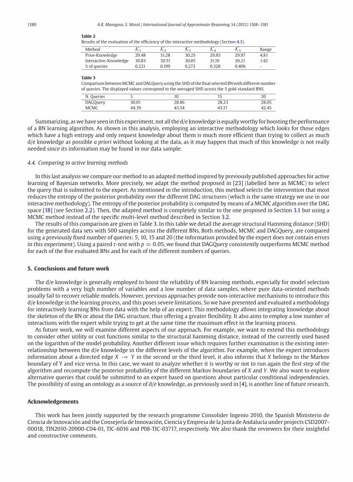
1180 A.R. Masegosa, S. Moral / International Journal of Approximate Reasoning 54 (2013) 1168–1181
Table 2
Results of the evaluation of the efficiency of the interactive methodology (Section 4.3).
Method K1 K2 K3 K4 K5 Range
Prior-Knowledge 29.48 31.28 30.25 29.85 29.97 4.81
Interactive-Knowledge 30.83 30.51 30.85 31.19 30.21 1.42
% of queries 0.221 0.199 0.273 0.328 0.406 -
Table 3
ComparisonbetweenMCMCandDAGQueryusing the SHDof thefinal selectedBNwithdifferent number
of queries. The displayed values correspond to the averaged SHD across the 5 gold-standard BNS.
N. Queries 5 10 15 20
DAGQuery 30.01 28.86 28.23 28.05
MCMC 44.39 43.54 43.17 42.45
Summarizing, aswehaveseen in this experiment,notall thed/eknowledge isequallyworthy forboosting theperformance
of a BN learning algorithm. As shown in this analysis, employing an interactive methodology which looks for those edges
which have a high entropy and only request knowledge about them is much more efficient than trying to collect as much
d/e knowledge as possible a priori without looking at the data, as it may happen that much of this knowledge is not really
needed since its information may be found in our data sample.
4.4. Comparing to active learning methods
In this last analysiswe compare ourmethod to an adaptedmethod inspired by previously published approaches for active
learning of Bayesian networks. More precisely, we adapt the method proposed in [23] (labelled here as MCMC) to select
the query that is submitted to the expert. As mentioned in the introduction, this method selects the intervention that most
reduces the entropy of the posterior probability over the different DAG structures (which is the same strategy we use in our
interactivemethodology). The entropy of the posterior probability is computed bymeans of aMCMC algorithm over the DAG
space [18] (see Section 2.2). Then, the adapted method is completely similar to the one proposed in Section 3.1 but using a
MCMC method instead of the specific multi-level method described in Section 3.2.
The results of this comparison are given in Table 3. In this table we detail the average structural Hamming distance (SHD)
for the generated data sets with 500 samples across the different BNs. Both methods, MCMC and DAGQuery, are compared
using a previously fixed number of queries: 5, 10, 15 and 20 (the information provided by the expert does not contain errors
in this experiment). Using a paired t-test with p = 0.05, we found that DAGQuery consistently outperforms MCMCmethod
for each of the five evaluated BNs and for each of the different numbers of queries.
5. Conclusions and future work
The d/e knowledge is generally employed to boost the reliability of BN learning methods, especially for model selection
problems with a very high number of variables and a low number of data samples, where pure data-oriented methods
usually fail to recover reliable models. However, previous approaches provide non-interactive mechanisms to introduce this
d/e knowledge in the learning process, and this poses severe limitations. Sowe have presented and evaluated amethodology
for interactively learning BNs from data with the help of an expert. This methodology allows integrating knowledge about
the skeleton of the BN or about the DAG structure, thus offering a greater flexibility. It also aims to employ a low number of
interactions with the expert while trying to get at the same time the maximum effect in the learning process.
As future work, we will examine different aspects of our approach. For example, we want to extend this methodology
to consider other utility or cost functions similar to the structural hamming distance, instead of the currently used based
on the logarithm of the model probability. Another different issue which requires further examination is the existing inter-
relationship between the d/e knowledge in the different levels of the algorithm. For example, when the expert introduces
information about a directed edge X → Y in the second or the third level, it also informs that X belongs to the Markov
boundary of Y and vice versa. In this case, we want to analyze whether it is worthy or not to run again the first step of the
algorithm and recompute the posterior probability of the different Markov boundaries of X and Y . We also want to explore
alternative queries that could be submitted to an expert based on questions about particular conditional independencies.
The possibility of using an ontology as a source of d/e knowledge, as previously used in [4], is another line of future research.
Acknowledgements
This work has been jointly supported by the research programme Consolider Ingenio 2010, the Spanish Ministerio de
Ciencia de Innovación and the Consejería de Innovación, Ciencia y Empresa de la Junta de Andalucía under projects CSD2007-
00018, TIN2010-20900-C04-01, TIC-6016 and P08-TIC-03717, respectively. We also thank the reviewers for their insightful
and constructive comments.

A.R. Masegosa, S. Moral / International Journal of Approximate Reasoning 54 (2013) 1168–1181 1181
References
[1] C.F. Aliferis, A.R. Statnikov, I. Tsamardinos, S. Mani, X.D. Koutsoukos, Local causal and Markov blanket induction for causal discovery and feature selectionfor classification part i: Algorithms and empirical evaluation, Journal of Machine Learning Research 11 (2010) 171–234.
[2] N. Angelopoulos, J. Cussens, Bayesian learning of Bayesian networkswith informative priors, Annals ofMathematics and Artificial Intelligence 54 (1) (2008)53–98.
[3] R. Bellazzi, B. Zupan, Towards knowledge-based gene expression data mining, Journal of Biomedical Informatics 40 (6) (2007) 787–802.[4] M. Ben Messaoud, P. Leray, N. Ben Amor, Integrating ontological knowledge for iterative causal discovery and visualization, Symbolic and Quantitative
Approaches to Reasoning with Uncertainty (2009) 168–179.
[5] G. Borboudakis, I. Tsamardinos. Incorporating causal prior knowledge as path-constraints in Bayesian networks and maximal ancestral graphs, arXivpreprint arXiv:1206.6390, 2012.
[6] W. Buntine, Theory refinement on Bayesian networks, in: Proceedings of the seventh conference on uncertainty in artificial intelligence, San Francisco, CA,USA, 1991, pp. 52–60.
[7] A. Cano, A. Masegosa, S. Moral, An importance sampling approach to integrate expert knowledge when learning Bayesian networks from data, in: IPMU’10,13th International Conference on Processing and Management of Uncertainty in Knowledge-Based Systems, Dortmund, Germany, June 28–July 2, 2010,
pp. 685–695.
[8] A. Cano, A. Masegosa, S. Moral, A method for integrating expert knowledge when learning Bayesian networks from data, IEEE Transactions on Systems,Man, and Cybernetics – Part B: Cybernetics 41 (2011) 1382–1394.
[9] D.M. Chickering, Optimal structure identification with greedy search, Journal of Machine Learning Research 3 (2003) 507–554.[10] L.M. de Campos, J.G. Castellano, Bayesian network learning algorithms using structural restrictions, International Journal of Approximate Reasoning 45 (2)
(2007) 233–254.[11] R.O. Duda, P.E. Hart, Pattern Classification and Scene Analysis, John Wiley Sons, New York, 1973.
[12] N. Friedman, D. Koller, Being Bayesian about Bayesian network structure: A Bayesian approach to structure discovery in Bayesian networks, Machine
Learning 50 (1–2) (2003) 95–125.[13] D. Heckerman, D. Geiger, D. Chickering, Learning Bayesian networks: the combination of knowledge and statistical data, Machine Learning 20 (3) (1995)
197–243.[14] M. Henrion, Propagating uncertainty by logic sampling in Bayes’ networks, in: J. Lemmer, L. Kanal (Eds.), Uncertainty in Artificial Intelligence, vol. 2,
Amsterdam, 1988, pp. 149–164.[15] S. Imoto, T. Higuchi, T. Goto, K. Tashiro, S. Kuhara, S. Miyano, Combining microarrays and biological knowledge for estimating gene networks via Bayesian
networks, in: CSB’03: Proceedings of the IEEE Computer Society Conference on Bioinformatics, IEEE Computer Society, Washington, DC, USA, 2003, p. 104.
[16] F.V. Jensen, Bayesian Networks and Decision Graphs. Statistics for Engineering and Information Science, Springer-Verlag, New York, USA, 2001.[17] B. Jones, C. Carvalho, A. Dobra, C. Hans, C. Carter, M.West, Experiments in stochastic computation for high dimensional graphical models, Statistical Science
20 (2004) 388–400.[18] D. Madigan, J. York, Bayesian graphical models for discrete data, International Statistical Review 63 (1995) 215–332.
[19] A.R. Masegosa, S. Moral, A Bayesian stochastic search method for discovering Markov boundaries, Knowledge-Based Systems 35 (2012) 211–223.[20] A.R. Masegosa, S. Moral, New skeleton-based approaches for Bayesian structure learning of Bayesian networks, Applied Soft Computing 13 (2) (2013)
1110–1120.[21] S. Meganck, P. Leray, B. Manderick, Learning causal Bayesian networks from observations and experiments: a decision theoretic approach, Modeling
Decisions for Artificial Intelligence (2006) 58–69.
[22] H.W. Mewes, D. Frishman, K.F.X. Mayer, M. Mnsterktter, O. Noubibou, T. Rattei, M. Oesterheld, V. Stmpflen, Mips: analysis and annotation of proteins fromwhole genomes, Nucleic Acids Research 32 (2004) 41–44.
[23] K.P. Murphy, Active learning of causal Bayes net structure, Technical report, 2001.[24] R.E. Neapolitan, Learning Bayesian Networks, Prentice Hall, 2004.
[25] H. Ogata, S. Goto, K. Sato, W. Fujibuchi, H. Bono, M. Kanehisa, Kegg: Kyoto encyclopedia of genes and genomes, Nucleic Acids Research 27 (1) (1999) 29–34.[26] J. Pearl, Probabilistic Reasoning with Intelligent Systems, Morgan & Kaufman, San Mateo, 1988.
[27] E. Perrier, S. Imoto, S. Miyano, Finding optimal Bayesian network given a super-structure, Journal of Machine Learning Research 9 (2008) 2251–2286.
[28] O. Pourret, P. Naim, B. Marco, Bayesian Networks: A Practical Guide to Applications, John Wiley Sons, New York, 2008.[29] M. Richardson, P. Domingos, Learningwith knowledge frommultiple experts, in:Machine Learning-InternationalWorkshop then Conference, vol. 20, 2003,
p. 624.[30] G. Scott, C.M. Carvalho, Feature-inclusion stochastic search for Gaussian graphical models, Journal of Computational and Graphical Statistics 17 (2008)
790–808.[31] J.G. Scott, J.O. Berger, An exploration of aspects of Bayesian multiple testing, Journal of Statistical Planning and Inference 136 (7) (2006) 2144–2162.
[32] P. Spirtes, C. Glymour, R. Scheines, Causation, Prediction and Search, Springer Verlag, Berlin, 1993.
[33] S. Tong, D. Koller, Active learning for structure in Bayesian networks, in: International Joint Conference on Artificial Intelligence, 2001, pp. 863–869.[34] I. Tsamardinos, L.E. Brown, C.F. Aliferis, The max–min hill-climbing Bayesian network structure learning algorithm, Machine Learning 65 (1) (2006) 31–78.