An Importance Sampling Approach to Integrate Expert Knowledge When Learning Bayesian Networks From...

An Importance sampling approach tointegrate expert knowledge when learning

Bayesian Networks from data

Andrés Cano, Andrés R. Masegosa and Serafín Moral

Department of Computer Science and Artificial Intelligence

University of Granada (Spain)

Dortmund, June 2010

Information Processing and Management of Uncertainty in Knowledge-Based Systems

IPMU 2010 Dortmund (Germany) 1/32

Outline

1 Introduction

2 Learning Bayesian Networks(BN) from data

3 Importance Sampling for learning BN

4 Integration of Expert Knowledge

5 Experimental Evaluation

6 Conclusions & Future Works

Introduction

Part I

Introduction

Bayesian Networks

Excellent models to graphically represent the dependency structure of theunderlying distribution in multivariate domains.

The learning from data of this dependency structure in a multivariate problemdomain represents a very relevant source of knowledge (direct interactions,conditional independencies...)

Introduction

Learning Bayesian Networks from Data

Uncertainty in Model Selection

When learning BNs from data there usually are several models with a highscore (high posterior probability given the data).

This situation is specially common in problem domains with high number ofvariables and low sample sizes.

Introduction

Integration of Expert Knowledge

Expert Knowledge

In many domain problems expert knowledge is available.

The graphical structure of BNs greatly ease the interaction with a human expert:

Causal ordering.D-separtion criteria.

Previous Works I

There have been many attempts to introduce expert knowledge when learningBNs from data.

Via Prior Distribution [2,5]: Use of specific prior distributions over thepossible graph structures to integrate expert knowledge:

Expert assigns higher prior probabilities to most likely edges.

Introduction

Expert Knowledge

In many domain problems expert knowledge is available.

The graphical structure of BNs greatly ease the interaction with a human expert:

Causal ordering.D-separtion criteria.

Previous Works I

There have been many attempts to introduce expert knowledge when learningBNs from data.

Via Prior Distribution [2,5]: Use of specific prior distributions over thepossible graph structures to integrate expert knowledge:

Expert assigns higher prior probabilities to most likely edges.

Introduction

Previous Works II

Via structural Restrictions [6]: Expert codify his/her knowledge as structuralrestrictions.

Expert defines the existence/absence of arcs and/or edges and causalordering restrictions.Retrieved model should satisfy these restrictions.

Limitations of "Prior" Expert Knowledge

The system would ask to the expert his/her belief about any possible featureof the BN (non feasible in high domains).

The expert could be biased to provide the most “easy” or clear knowledge.

The system does not help to the user to introduce information about the BNstructure.

Introduction

Previous Works II

Via structural Restrictions [6]: Expert codify his/her knowledge as structuralrestrictions.

Expert defines the existence/absence of arcs and/or edges and causalordering restrictions.Retrieved model should satisfy these restrictions.

Limitations of "Prior" Expert Knowledge

The system would ask to the expert his/her belief about any possible featureof the BN (non feasible in high domains).

The expert could be biased to provide the most “easy” or clear knowledge.

The system does not help to the user to introduce information about the BNstructure.

Introduction

Interactive Learning of Bayesian Networks

Active Interaction with the Expert

Strategy: Ask to the expert by the presence of the edges that most reduce themodel uncertainty.

Method: Framework to allow an efficient and effective interaction with the expert.

Expert is only asked for this controversial structural features.

Introduction

Interactive Learning of Bayesian Networks

Active Interaction with the Expert

Strategy: Ask to the expert by the presence of the edges that most reduce themodel uncertainty.

Method: Framework to allow an efficient and effective interaction with the expert.

Expert is only asked for this controversial structural features.

Previous Knowledge

Part II

Learning Bayesian Networks from data

Previous Knowledge

Notation

Let be X = (X1, ...,Xn) a set of n random variables. Val(Xi ) is the set of valuesof Xi .

We assume variables are enumerated in a total causal order.We also assume a fully observed data set D.

A Bayesian Network B can be described by:

G the graph structure.θG the parameters.

A graph G can be decomposed as a vector of parent sets:

G = (Pa(X1), ...,Pa(Xn))

We also define Ui as a random variable taking values in the space of all possibleparent sets of Xi , Val(Ui ).

Let be G a random variable taking values in the set Val(G) of all possible graphstructures consistent with the total order.

Previous Knowledge

Notation

G = (Pa(X1), ...,Pa(Xn))

Previous Knowledge

Notation

G = (Pa(X1), ...,Pa(Xn))

Previous Knowledge

The Bayesian Learning Framework

Scoring a graph structure

Marginal Likelihood of a graph structure:

P(G = G|D) = P(G|D) ∝ P(G)P(D|G) =∏

score(Xi ,PaG(Xi )|D)

scoreBDeu(Xi ,Ui |D) = Pi (U)

|Ui |∏j=0

Γ(αij )

Γ(αij + Nij )

|Xi |∏k=1

Γ(αijk + Nijk )

Γ(αijk )

Pi (U) is the prior probability that U is the parent set of Xi .

Approximating the posterior P(G|D)

Our approach is supported on the approximation of P(G|D).

It allows to know which graph structures are the most likely (best explain thedata).

Exhaustive enumeration is not feasible because the space of graph structures issuper-exponential.

Previous Knowledge

The Bayesian Learning Framework

Scoring a graph structure

Marginal Likelihood of a graph structure:

P(G = G|D) = P(G|D) ∝ P(G)P(D|G) =∏

score(Xi ,PaG(Xi )|D)

scoreBDeu(Xi ,Ui |D) = Pi (U)

|Ui |∏j=0

Γ(αij )

Γ(αij + Nij )

|Xi |∏k=1

Γ(αijk + Nijk )

Γ(αijk )

Pi (U) is the prior probability that U is the parent set of Xi .

Approximating the posterior P(G|D)

Our approach is supported on the approximation of P(G|D).

It allows to know which graph structures are the most likely (best explain thedata).

Exhaustive enumeration is not feasible because the space of graph structures issuper-exponential.

Previous Knowledge

Approximating the Posterior

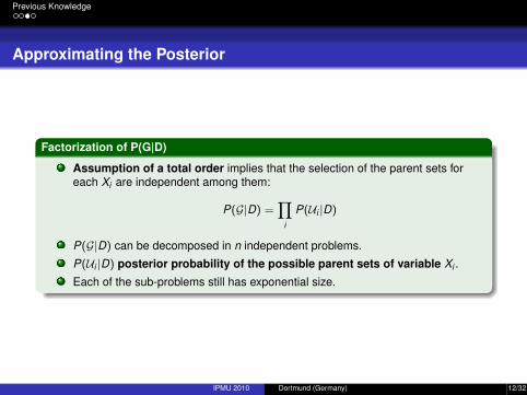
Factorization of P(G|D)

Assumption of a total order implies that the selection of the parent sets foreach Xi are independent among them:

P(G|D) =∏

P(Ui |D)

P(G|D) can be decomposed in n independent problems.

P(Ui |D) posterior probability of the possible parent sets of variable Xi .

Each of the sub-problems still has exponential size.

Previous Knowledge

Approximating the Posterior P(Ui |D)

Closed Form Solution

In [3] it was proposed a closed form solution assuming a node can have up toK parents.

It would have a polynomial efficiency O(n(K +1)).

Markov Chain Monte Carlo

Lets Val(Ui ) be the space model of the Markov Chain.

If the Markov Chain is in some state U in iteration t , a new model U′ israndomly drawn by adding, deleting of switching any edge.

The Markov Chain moves to state U′ in the iteration t + 1 with probability:

m(Ut ,Ut+1) = min{1,N (U)score(D|U′)N (U′)score(D|U)

If it not, the Markov Chain remains in state U.

This Markov Chain has an stationary distribution (t →∞) which is P(U|D).

Previous Knowledge

Approximating the Posterior P(Ui |D)

Closed Form Solution

In [3] it was proposed a closed form solution assuming a node can have up toK parents.

It would have a polynomial efficiency O(n(K +1)).

Markov Chain Monte Carlo

Lets Val(Ui ) be the space model of the Markov Chain.

If the Markov Chain is in some state U in iteration t , a new model U′ israndomly drawn by adding, deleting of switching any edge.

The Markov Chain moves to state U′ in the iteration t + 1 with probability:

m(Ut ,Ut+1) = min{1,N (U)score(D|U′)N (U′)score(D|U)

If it not, the Markov Chain remains in state U.

This Markov Chain has an stationary distribution (t →∞) which is P(U|D).

Importance Sampling

Part III

Importance Sampling

Description

Based on the employment of an auxiliary distribution Q which roughlyapproximate P, the target distribution.

Q is a distribution which is easier to sample for it.

EP(f (x)) =

∫P(x)

Q(x)f (x)Q(x)dx = EQ(w(x)f (x)) (1)

where w(x) = P(x)Q(x)

acts as a weight function.

A set of T samples {x1, ..., xT } are generated form Q and, then, it is computed

w t = P(x t )

Q(x t ).

The estimator µ̂ of EP(f (x)) is finally computed as follows:

µ̂ =

∑Tt=1 w(x t )f (t)∑T

t=1 w(x t )(2)

Key Aspect: P and Q can be known up to a multiplicative constant.

Importance Sampling

Description

Based on the employment of an auxiliary distribution Q which roughlyapproximate P, the target distribution.

Q is a distribution which is easier to sample for it.

EP(f (x)) =

∫P(x)

Q(x)f (x)Q(x)dx = EQ(w(x)f (x)) (1)

where w(x) = P(x)Q(x)

acts as a weight function.

A set of T samples {x1, ..., xT } are generated form Q and, then, it is computed

w t = P(x t )

Q(x t ).

The estimator µ̂ of EP(f (x)) is finally computed as follows:

µ̂ =

∑Tt=1 w(x t )f (t)∑T

t=1 w(x t )(2)

Key Aspect: P and Q can be known up to a multiplicative constant.

Importance Sampling

Importance Sampling for learning BNs

Step 0:

Candidate Parents are considered in arandom permutation.

Score of initial model:

score(X , {∅}|D)

Importance Sampling

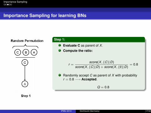
Step 1:

Evaluate C as parent of X .

Compute the ratio:

r =score(X , {C}|D)

score(X , {C}|D) + score(X , {∅}|D)= 0.8

Randomly accept C as parent of X with probabilityr = 0.8 −→ Accepted.

Q = 0.8

Importance Sampling

Step 2:

Evaluate B as parent of X .

Compute the ratio:

r =score(X , {C,B}|D)

score(X , {C,B}|D) + score(X , {C}|D)= 0.1

Randomly accept B as parent of X with probabilityr = 0.1 −→ Non Accepted.

Q = 0.8 · 0.9

Importance Sampling

Step 3:

Evaluate A as parent of X .

Compute the ratio:

r =score(X , {C,A}|D)

score(X , {C,A}|D) + score(X , {C}|D)= 0.7

Randomly accept A as parent of X with probabilityr = 0.7 −→ Accepted.

Q = 0.8 · 0.9 · 0.7 = 0.504

Weight of the final model:

W 1 =score(X , {C,A}|D)

The process is repeated T times.

Using these samples we get an approximation of P(Ui |D).

Importance Sampling

Step 3:

Evaluate A as parent of X .

Compute the ratio:

r =score(X , {C,A}|D)

score(X , {C,A}|D) + score(X , {C}|D)= 0.7

Randomly accept A as parent of X with probabilityr = 0.7 −→ Accepted.

Q = 0.8 · 0.9 · 0.7 = 0.504

Weight of the final model:

W 1 =score(X , {C,A}|D)

The process is repeated T times.

Using these samples we get an approximation of P(Ui |D).

Integrating Expert Knowledge

Part IV

Methodology Description

Prior Knowledge

Representing absence of prior knowledge

“Uniform prior over structures is usually chosen by convenience” [3].

P(G) does not grow with the data, but it matters at low sample sizes.

Let us assume that the prior probability of an edge is p and independent ofeach other. If Xi has k parents out of m nodes:

P(Pa(Xi )) = pk (1− p)(m−k)

If the number of candidate parents m grows, p should be decreased tocontrol de number of false positives edges: “multiplicity correction”.

This is solved by assuming that p has a Beta prior with parameter α = 0.5 [11]:

Pi (Pa(Xi )) =Γ(2 ∗ α)

Γ(m + 2α)

Γ(k + α)Γ(m − k + α)

Γ(α)Γ(α)

Prior Knowledge

P(Pa(Xi )) = pk (1− p)(m−k)

Pi (Pa(Xi )) =Γ(2 ∗ α)

Γ(m + 2α)

Γ(k + α)Γ(m − k + α)

Γ(α)Γ(α)

Prior Knowledge

P(Pa(Xi )) = pk (1− p)(m−k)

Pi (Pa(Xi )) =Γ(2 ∗ α)

Γ(m + 2α)

Γ(k + α)Γ(m − k + α)

Γ(α)Γ(α)

Interacting with the Expert

P(S → X |D) = 0.85 P(R → X |D) = 0.8 P(C→ X|D) = 0.45

Description

Key Idea: As lower the entropy of P(Ui |D) is, more reliable learning we have.

Expert Interaction is carried out in order to reduce the entropy H(P(Ui |D)).

System ask to the expert by those edges with higher entropy

P(S → X |D) = 0.85 P(R → X |D) = 0.8 P(C→ X|D) = 0.45

Description

Key Idea: As lower the entropy of P(Ui |D) is, more reliable learning we have.

Expert Interaction is carried out in order to reduce the entropy H(P(Ui |D)).

System ask to the expert by those edges with higher entropy.

P(S → X |D) = 0.88 P(R → X |D) = 0.77 P(C→ X|D) = 1.0

Description

The entropy of P(Ui |D) is reduced. Probability mass concentrates aroundone model.This methodology can be iteratively applied asking by the presence/absenceof more edges.

Stopping the interaction when the probability of MAP model is L times higherthe second most probable model.

Experimental Evaluation

Part V

Experimental Set-up

Bayesian Networks:

alarm (37 nodes), boblo (23 nodes), boerlage-92 (23 nodes), hailfinder (56nodes), insurance (27 nodes).

Sample Sizes:

We run 10 times the algorithms with different samples sizes: 50, 100, 500and 1000.

Evaluation Measures

Number of missing/extra links, Kullback-Leibler distance...We report average values across the five networks.

Expert Interaction is simulated:

Access to the true BN model when asking bypresence/absence of an edge.

Experimental Set-up

Bayesian Networks:

alarm (37 nodes), boblo (23 nodes), boerlage-92 (23 nodes), hailfinder (56nodes), insurance (27 nodes).

Sample Sizes:

We run 10 times the algorithms with different samples sizes: 50, 100, 500and 1000.

Evaluation Measures

Number of missing/extra links, Kullback-Leibler distance...We report average values across the five networks.

Expert Interaction is simulated:

Access to the true BN model when asking bypresence/absence of an edge.

Structure Prior Evaluation

N. of Structural Errors KL Distance

Analysis

Beta-Prior reduces the number of structural errors for both IS and MCMCM.

IS has a low number of errors than MCMC specially with low sample sizes.

Beta-Prior also reduces KL distance for both IS and MCMC.

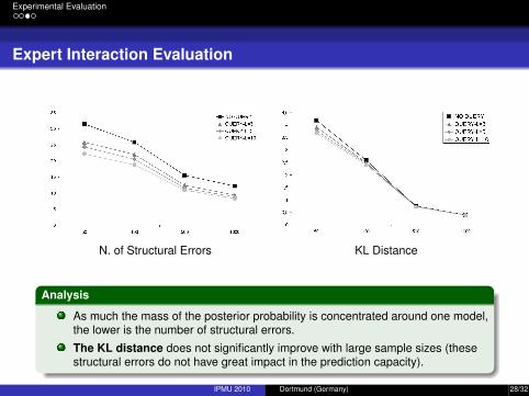
Expert Interaction Evaluation

N. of Structural Errors KL Distance

Analysis

As much the mass of the posterior probability is concentrated around one model,the lower is the number of structural errors.

The KL distance does not significantly improve with large sample sizes (thesestructural errors do not have great impact in the prediction capacity).

Expert Interaction Evaluation

N. of Interactions Interaction Accuracy

Analysis

The number of Interactions are feasible for a human expert.

Prior Exhaustive Querying: 600 questions in averaged.

The Interaction Accuracy: ratio between number of reduced structuralerrors and number of interactions.

Average Accuracy of random interactions: 1%.

Conclusions

Part VI

Conclusions & Future Works

Conclusions

A new methodology to introduce expert knowledge whenlearning BN from data.

A new Importance sampling technique for sampling BN.

System requests to the expert a feasible number of questions.

Interaction improves the quality of the inferred BN models.

Future Works

Extend these methods to the learning of BN models withoutcausal ordering assumptions.

Conclusions

A new methodology to introduce expert knowledge whenlearning BN from data.

A new Importance sampling technique for sampling BN.

System requests to the expert a feasible number of questions.

Interaction improves the quality of the inferred BN models.

Future Works

Extend these methods to the learning of BN models withoutcausal ordering assumptions.

Thanks for your attention!!

Questions?

An Importance Sampling Approach to Integrate Expert Knowledge When Learning Bayesian Networks From...

Science

Transcript of An Importance Sampling Approach to Integrate Expert Knowledge When Learning Bayesian Networks From...