An Integrated Framework for Coupling Traffic and · PDF fileAn Integrated Framework for...
130
An Integrated Framework for Coupling Traffic and Wireless Network Simulations by Yassmin Shalaby A thesis submitted in conformity with the requirements for the degree of Master of Applied Science Graduate Department of Civil Engineering University of Toronto Copyright c 2010 by Yassmin Shalaby
Transcript of An Integrated Framework for Coupling Traffic and · PDF fileAn Integrated Framework for...

An Integrated Framework for Coupling Traffic andWireless Network Simulations
by
Yassmin Shalaby
A thesis submitted in conformity with the requirementsfor the degree of Master of Applied ScienceGraduate Department of Civil Engineering
University of Toronto
Copyright c© 2010 by Yassmin Shalaby

Abstract
An Integrated Framework for Coupling Traffic and Wireless Network Simulations
Yassmin Shalaby
Master of Applied Science
Graduate Department of Civil Engineering
University of Toronto
2010
Intelligent Transportation Systems (ITS) include a wide range of applications that aim
to use state-of-the-art communication and information technologies to enhance and con-
trol the flow of traffic. The ability to communicate with cars while travelling on the
road is crucial to the success of these systems and thus requires careful studying. This
research aims to study the feasibility of deploying wireless communication networks that
are capable of collecting data from cars as well as providing them with information about
the current traffic situation. We present a platform that integrates a microscopic traffic
simulation, Paramics, and a communication network simulator, Omnet++. The inte-
gration of both simulators is a key solution to several research problems both on the
communications side and on the transportation side. The combined simulator will allow
designing and testing ITS Applications, which rely on communication between vehicles,
before they are implemented on the streets.
ii

Dedication
In the name of Allah most gracious, most merciful.
All my success is due to Allah; in Him I trust and unto Him I look.
To my wonderful parents who guided me to the path of success and allowed me to
discover new oceans.
To my siblings and my grandparents whose love and support is endless.
To all my friends and family members who kept me motivated.
Finally, to my beloved husband, Zyad who shared with me all the tough moments with
patience, love and tenderness.
iii

Acknowledgements
I would like to express my deep gratitude towards my supervisors, Professor Baher
Abdulhai and Professor Mohamed El-Darieby, for their continuous guidance and advice
in my research and academic work.
I wish to thank my colleague Hossam Abdel Gawad who has provided guidance and
data for the research work.
Special thanks to the alumni Hoda Talaat and Mohamed Masoud for their time and
help.
My sincerest thanks to my friend and lab mate Samah Eltantawy for her knowledge
and support.
I would like to thank the instructors at the English Language and Writing Support
(ELWS) at the University of Toronto for providing international students with
outstanding courses.
Also, many thanks to the individuals at the Academic Editing Service for editing my
thesis.
Last, but not least, I express my warm appreciation to my beloved husband, Zyad who
has always been there for me through the hard times and the happy moments.
iv

Contents
1 Introduction 1
1.1 Overview . . . . . . . . . . . . . . . . . . . . . . . . . . . . . . . . . . . . 1
1.2 Motivation . . . . . . . . . . . . . . . . . . . . . . . . . . . . . . . . . . . 3
1.2.1 Modeling Vehicular Mobility in Wireless Network Simulators . . . 3
1.2.2 Feeding Back Data from Wireless Network Simulators into Traffic
Simulators . . . . . . . . . . . . . . . . . . . . . . . . . . . . . . . 4
1.3 Contributions . . . . . . . . . . . . . . . . . . . . . . . . . . . . . . . . . 5
1.3.1 Importing Vehicular Mobility Traces into Wireless Network Simu-
lators . . . . . . . . . . . . . . . . . . . . . . . . . . . . . . . . . . 6
1.3.2 Allowing Intercommunication between Wireless Network Simula-
tors and Traffic Simulators . . . . . . . . . . . . . . . . . . . . . . 7
1.4 Organization of Thesis . . . . . . . . . . . . . . . . . . . . . . . . . . . . 7
2 Background 9
2.1 Introduction . . . . . . . . . . . . . . . . . . . . . . . . . . . . . . . . . . 9
2.2 Traffic Networks . . . . . . . . . . . . . . . . . . . . . . . . . . . . . . . . 11
2.2.1 Traffic Flow Modeling . . . . . . . . . . . . . . . . . . . . . . . . 11
2.2.2 Traffic Network Simulation Categories . . . . . . . . . . . . . . . 13
2.2.3 Properties of Microscopic Traffic Simulators . . . . . . . . . . . . 15
2.3 Wireless Networks . . . . . . . . . . . . . . . . . . . . . . . . . . . . . . 17
v

2.3.1 Wireless Network Modeling . . . . . . . . . . . . . . . . . . . . . 17
2.3.2 Wireless Network Simulators . . . . . . . . . . . . . . . . . . . . . 21
3 Related Work 25
3.1 Introduction . . . . . . . . . . . . . . . . . . . . . . . . . . . . . . . . . . 25
3.2 Utilizing Wireless Communication in ITS Applications . . . . . . . . . . 26
3.2.1 Vehicular Network Access . . . . . . . . . . . . . . . . . . . . . . 26
3.2.2 Intelligent Vehicular Ad Hoc Networks (InVANET) . . . . . . . . 29
3.3 Representing Vehicular Movement in Wireless Network Simulators . . . . 31
3.3.1 Using Mathematical Models to Generate Mobility Traces . . . . . 32
3.3.2 Extracting Mobility Traces from Road Traffic Simulators . . . . . 33
3.4 Incorporating Wireless Communications in Traffic Network Simulators . . 36
3.4.1 Merging Traffic and Wireless Simulators . . . . . . . . . . . . . . 36
3.4.2 Creating a New Platform . . . . . . . . . . . . . . . . . . . . . . . 38
4 Coupling Paramics to OMNeT++ 39
4.1 Introduction . . . . . . . . . . . . . . . . . . . . . . . . . . . . . . . . . . 39
4.2 Paramics and OMNeT++ . . . . . . . . . . . . . . . . . . . . . . . . . . 40
4.2.1 Paramics . . . . . . . . . . . . . . . . . . . . . . . . . . . . . . . . 40
4.2.2 OMNeT++ . . . . . . . . . . . . . . . . . . . . . . . . . . . . . . 42
4.3 Offline Coupling of Paramics and OMNeT++ . . . . . . . . . . . . . . . 46
4.3.1 Paramics Simulation . . . . . . . . . . . . . . . . . . . . . . . . . 46
4.3.2 OMNeT++ Simulation . . . . . . . . . . . . . . . . . . . . . . . . 51
4.3.3 Applications of Offline Coupling . . . . . . . . . . . . . . . . . . . 54
4.4 Online Coupling of Paramics and OMNeT++ . . . . . . . . . . . . . . . 55
4.4.1 Overview . . . . . . . . . . . . . . . . . . . . . . . . . . . . . . . 56
4.4.2 Paramics Plugin . . . . . . . . . . . . . . . . . . . . . . . . . . . . 57
4.4.3 OMNeT++ Wireless Network . . . . . . . . . . . . . . . . . . . . 71
vi

4.4.4 Discussion . . . . . . . . . . . . . . . . . . . . . . . . . . . . . . . 79
4.4.5 Applications of Online Coupling . . . . . . . . . . . . . . . . . . . 81
5 Case Studies 82
5.1 Introduction . . . . . . . . . . . . . . . . . . . . . . . . . . . . . . . . . . 82
5.2 Testing Scenario . . . . . . . . . . . . . . . . . . . . . . . . . . . . . . . . 83
5.3 Measurement criteria . . . . . . . . . . . . . . . . . . . . . . . . . . . . . 85
5.3.1 Adjusting parameters . . . . . . . . . . . . . . . . . . . . . . . . . 85
5.3.2 Performance metrics . . . . . . . . . . . . . . . . . . . . . . . . . 88
5.4 Case Studies . . . . . . . . . . . . . . . . . . . . . . . . . . . . . . . . . . 90
5.4.1 Expressway Congestion . . . . . . . . . . . . . . . . . . . . . . . . 93
5.4.2 Surface Street Accident . . . . . . . . . . . . . . . . . . . . . . . . 101
6 Conclusions and Future Recommendations 110
6.1 Summary . . . . . . . . . . . . . . . . . . . . . . . . . . . . . . . . . . . 110
6.2 Future Work . . . . . . . . . . . . . . . . . . . . . . . . . . . . . . . . . . 111
6.2.1 Modifications . . . . . . . . . . . . . . . . . . . . . . . . . . . . . 112
6.2.2 Applications . . . . . . . . . . . . . . . . . . . . . . . . . . . . . . 113
Bibliography 114
vii

List of Tables
5.1 Paramics Queens Quay Network data . . . . . . . . . . . . . . . . . . . . 92
5.2 Comparison of the specifications of accidentLink and alternateLink . . . 94
5.3 Parameters of experiment 1-1 . . . . . . . . . . . . . . . . . . . . . . . . 95
5.4 Parameters of experiment 1-2 . . . . . . . . . . . . . . . . . . . . . . . . 100
5.5 Comparison of the specifications of accidentLink and alternateLink . . . 101
5.6 Parameters of experiment 2-1 . . . . . . . . . . . . . . . . . . . . . . . . 103
5.7 Parameters of experiment 2-2 . . . . . . . . . . . . . . . . . . . . . . . . 108
viii

List of Figures
2.1 Intercommunication is needed between traffic network simulators and wire-
less network simulators . . . . . . . . . . . . . . . . . . . . . . . . . . . 10
2.2 Fundamental diagram showing the relationships between flow, density and
speed (ideal conditions) [35][modified]. . . . . . . . . . . . . . . . . . . . 12
2.3 Illustration of shock waves [source: Lecture Notes]. . . . . . . . . . . . . 12
2.4 Traffic Simulation Software Classification [source: Lecture Notes]. . . . . 14
2.5 A snapshot from a traffic network simulator (Paramics). . . . . . . . . . 17
2.6 Wireless Network Modeling [27][modified]. . . . . . . . . . . . . . . . . . 18
2.7 Implementing a wireless system on the road. . . . . . . . . . . . . . . . 21
2.8 Wireless Host Module implemented by [25]. . . . . . . . . . . . . . . . . 22
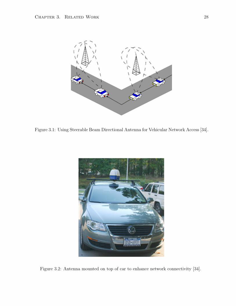
3.1 Using Steerable Beam Directional Antenna for Vehicular Network Ac-
cess [34]. . . . . . . . . . . . . . . . . . . . . . . . . . . . . . . . . . . . 28
3.2 Antenna mounted on top of car to enhance network connectivity [34]. . 28
4.1 Coupling Paramics to OMNeT++. . . . . . . . . . . . . . . . . . . . . . 40
4.2 An example of a simple OMNeT++ network simulation (by INET frame-
work [25]). . . . . . . . . . . . . . . . . . . . . . . . . . . . . . . . . . . 44
4.3 Offline Coupling. . . . . . . . . . . . . . . . . . . . . . . . . . . . . . . . 47
4.4 A Paramics traffic network showing part of the Queens Quay network in
downtown Toronto. . . . . . . . . . . . . . . . . . . . . . . . . . . . . . 48
ix

4.5 A snapshot of the original file (mobility-traces.csv) output from Paramics
showing the mobility traces of all vehicles throughout the simulation. . . 49
4.6 A snapshot of the factory.xml file showing the initial and final position of
each vehicle. . . . . . . . . . . . . . . . . . . . . . . . . . . . . . . . . . 50
4.7 A snapshot of the mobility-traces.xml file showing the mobility traces of
all vehicles throughout the simulation. . . . . . . . . . . . . . . . . . . . 50
4.8 Online Coupling. . . . . . . . . . . . . . . . . . . . . . . . . . . . . . . . 55
4.9 Communications between Paramics and OMNeT++. . . . . . . . . . . . 58
4.10 Flowchart of “callOmnet” plugin. . . . . . . . . . . . . . . . . . . . . . . 62
4.11 Snapshot of files exchanged between Paramics and OMNeT++. . . . . . 64
4.12 Cars communicating in an Ad Hoc manner. . . . . . . . . . . . . . . . . 73
4.13 The top figure shows the car-to-car mode while the bottom figure shows
the car-to-infrastructure mode. . . . . . . . . . . . . . . . . . . . . . . . 74
4.14 Broadcasting a message to all cars within range. . . . . . . . . . . . . . 75
4.15 Wireless car module. . . . . . . . . . . . . . . . . . . . . . . . . . . . . . 78
4.16 Snapshot of “TalkToParamics” simulation running on OMNeT++ plat-
form. . . . . . . . . . . . . . . . . . . . . . . . . . . . . . . . . . . . . . 80
5.1 Illustration of accident scenario. . . . . . . . . . . . . . . . . . . . . . . 84
5.2 Study area: Queens Quay West, Toronto, ON, Canada (Google Maps) . . 90
5.3 Paramics Network: Queens Quay . . . . . . . . . . . . . . . . . . . . . . 91
5.4 Zoomed area of Queens Quay map showing the positions of the two accidents 92
5.5 Accident on Gardiner [Google Maps] . . . . . . . . . . . . . . . . . . . . 93
5.6 Gardiner Accident in Paramics network . . . . . . . . . . . . . . . . . . . 93
5.7 Average Queue Length for different compliance factors . . . . . . . . . . 95
5.8 Average Total Travel Time for different compliance factors . . . . . . . . 96
5.9 Optimal Diversion Ratio . . . . . . . . . . . . . . . . . . . . . . . . . . . 97
5.10 Bar Chart of average total travel time in 4 different cases. . . . . . . . . 98
x

5.11 Comparison with average total travel time over whole network . . . . . . 99
5.12 Effect of sending time interval on number of messages received and on
total CPU time elapsed. . . . . . . . . . . . . . . . . . . . . . . . . . . . 101
5.13 Accident on Front St. W [Google Maps] . . . . . . . . . . . . . . . . . . 102
5.14 Surface Street Accident on Paramics network . . . . . . . . . . . . . . . . 102
5.15 Average Queue Length for different compliance factors . . . . . . . . . . 104
5.16 Average Total Travel Time for different compliance factors . . . . . . . . 105
5.17 Optimal Diversion Ratio . . . . . . . . . . . . . . . . . . . . . . . . . . . 106
5.18 Bar Chart of average total travel time in 4 different cases. . . . . . . . . 106
5.19 Comparison with average total travel time over whole network . . . . . . 107
5.20 Effect of sending time interval on number of messages received and on
total CPU time elapsed. . . . . . . . . . . . . . . . . . . . . . . . . . . . 109
xi
Chapter 1
Introduction
1.1 Overview
A successful transportation system contributes directly to the progress of societies. De-
ficient transportation systems can cause people to spend a great portion of their time in
traffic jams wasting their time and effort, and contributing to an increase in the level of
air pollution. This can result in lower individual productivities, higher levels of pollution
and even negative impacts on social life.
On the other hand, building a successful transportation system is a daunting task, that
requires attentive planning and management to optimize the overall performance of the
system. The success of a transportation system is characterized by safe and smooth traffic
flow with minimum congestion bottlenecks, together with the lowest possible level of
pollution emitted. Traffic congestion, the principal reason for hindering the performance
of transportation systems, occurs because of the increased demand for travel with limited
increase in supply of the transportation infrastructure. In an attempt to solve this
problem, Intelligent Transportation Systems (ITS) have emerged. ITS include a wide
range of applications which aim to control and adjust the flow of traffic in order to improve
safety, enhance travel times, reduce fuel consumption and provide seamless transportation
1

Chapter 1. Introduction 2
by using state-of-the-art communication and information technologies.
According to the Research And Innovative Technology Administration (RITA) [26],
there are 16 types of technical systems on which ITS applications are built. These systems
fall under one of two categories, intelligent infrastructure or intelligent vehicles. Intel-
ligent infrastructure systems are concerned with the management of arterials, freeways,
transits, traffic incidents, emergencies, electronic payment and pricing, road weather as
well as information management. Moreover, they provide traveler information, crash
prevention and safety and intermodal freight. On the other hand, intelligent vehicular
systems include collision avoidance, driver assistance and collision notification. The com-
mon factor in all these applications is the urgent requirement to gather real-time traffic
information, process this information and give feedback to the user whenever necessary.
Currently deployed methods used for gathering such information from roads include
point detectors for surveillance together with wired communication networks for informa-
tion transmission. Advanced Traffic Management Systems (ATMS)[46], for example,use
hard-wired surveillance equipment such as video surveillance and magnetic loop detectors
to provide: (i) traffic surveillance to assess current conditions, (ii) signals optimization
and (iii) ramp metering. Also, it is common to use optical fiber networks to transmit traf-
fic information from the roads to a central server in such management systems. However,
according to [46], installing and maintaining such a system requires about $5 billion per
year. The unreliability of loop detectors together with the high cost needed for building
and maintaining a wired network, directs researchers to find alternative methods for car
surveillance and traffic data collection.
Recently, wireless communication has been proposed for use in ITS applications. It
is anticipated that the use of wireless networks, in contrast to wired networks, would
reduce the total cost required for maintaining the system and would also facilitate up-
grades. Moreover, in many cases wireless networks can be more reliable than wired
systems. To clarify, in a typical wireless network consisting of a group of nodes commu-

Chapter 1. Introduction 3
nicating together, redundancy is assured such that if a node fails, the other nodes would
compensate for this failure. In order to offer the same redundancy in wired networks, a
huge cost would be involved.
1.2 Motivation
This section demonstrates the motivation behind the work performed in this thesis. Two
different yet closely related problems are being tackled. The first problem is related to
wireless network simulators, which are used to test the feasibility of wireless applications
in a vehicular environment. Existing simulators lack accurate modeling of vehicle move-
ment. The other problem is concerned with the modeling of newly emerging vehicular
communication systems. These systems utilize wireless communications in various traf-
fic applications and need to be modeled with a double edged simulator which combines
the capabilities of both wireless network simulators and traffic network simulators. Sec-
tion 1.2.1 explains the need for vehicular mobility modeling in wireless network simulators
and Section 1.2.2 illustrates the importance of integrating these two types of simulators.
1.2.1 Modeling Vehicular Mobility in Wireless Network Simu-
lators
Researchers are exploring the idea of providing internet access to moving vehicles [17, 13]
and are studying the use of vehicles as probes to collect data from the roads [12, 24].
Both the facility of providing vehicular internet access and the functionality of using
cars as probes, have to be supported by fixed Wireless Local Area Networks (WLAN)
such as 802.11 (Wi-Fi) [17] or by Wireless Personal Area Networks (WPAN) such as
802.15 (Bluetooth) [12]. These networks would typically consist of a group of wireless
access points mounted on street lamps that are capable of communicating with the cars,
collecting information from them, providing them with applications such as internet

Chapter 1. Introduction 4
browsing, voice over IP (VOIP) or even allowing them to download videos or movies
while on their way. However, design parameters such as the optimum distance between
access points, their positions and number, as well as the transmission power that would
satisfy the coverage area, need to be decided. It is essential to design this system using
wireless communication simulators before deploying it on roads. But, since protocols
such as 802.11 and 802.15 were primarily designed for applications with limited or no
mobility, the mobility models within these simulators, like constant speed model, linear
or circular motion models, are trivial compared to vehicular movement.
There is no doubt that testing these protocols in vehicular environments using these
simple mobility models leads to erroneous and misleading results. For example, assuming
that all cars on the highway are moving with constant speed at all times or assuming
that cars moving on arterial streets are continuously moving and not stopping at traffic
lights, could give optimistic results about the design of the wireless network, showing
that only 1 access point is enough to cover a 10 km district. While, actually, when this
system is deployed on the road, only a 5 km district would be covered due to the increased
interference at traffic lights.
In summary, there is an urgent need to model the movement of vehicles accurately in
simulations that deal with the design and performance of wireless vehicular networks.
1.2.2 Feeding Back Data from Wireless Network Simulators
into Traffic Simulators
The applications mentioned in Section 1.2.1 use wireless communication to provide ser-
vices to moving vehicles such as internet access and the downloading of files or videos.
The data sent to vehicles in these services do not carry any information about traffic
conditions and therefore simulations for these applications do not need to model the
driver responses to information received. On the other hand, there exists another cate-
gory of ITS applications which requires a change in the driver’s behavior, based on the

Chapter 1. Introduction 5
information received. For example, the Advanced Traveler Information System (ATIS)
is an ITS application that allows users to make decisions regarding alternate routes and
expected arrival times using real-time traffic information that is sent to drivers on de-
mand. Also, safety applications such as Intersection Collision Warning Systems warn
vehicles of approaching cross traffic and Road Geometry Warning Systems warn drivers,
especially those in heavy vehicles, of potentially dangerous conditions that may cause
rollovers or other crashes on ramps, curves, or downgrades [26]. In order to examine the
wireless network performance in these kinds of applications and to test the impact of
using these applications for improving the traffic situation, a special type of simulation is
needed. This simulation should integrate the capabilities of both traffic microsimulation
and wireless communication simulation.
Microscopic traffic simulation software simulates the behavior of all the individual
vehicles on a traffic network. On the other hand, wireless communication simulators are
qualified to model wireless communication protocols. The problem lies in the fact that
available microscopic traffic simulation software lacks wireless communication modeling
and at the same time wireless simulators are incapable of modeling a complete traffic
network.
In conclusion, there is an urgent need for simulators that are capable of combin-
ing the benefits of both wireless communication network simulators and traffic network
simulators.
1.3 Contributions
This section outlines the path followed towards the goal of solving the research problems
discussed in Section 1.2. To achieve this objective, we coupled a microscopic traffic
simulator, Paramics, to a wireless network simulator, OMNeT++. Section 1.3.1 explains
the steps taken towards providing an accurate vehicular mobility model to OMNeT++.

Chapter 1. Introduction 6
Section 1.3.2 demonstrates the method applied to provide intercommunication between
Paramics and OMNeT++.
1.3.1 Importing Vehicular Mobility Traces into Wireless Net-
work Simulators
In an attempt to fulfill the need for accurate mobility models to represent the movement
of vehicles in wireless communication simulators, we propose to use real mobility traces
of vehicles moving on the road. Mobility traces refer to the detailed path which vehicles
follow during their travel trip. Fortunately, it is possible to provide the vehicular mobility
model to the wireless communication simulator, OMNeT++, in the form of mobility
traces. These mobility traces can either come from GPS data associated with a certain
trip or more generally from microscopic traffic simulators. Microscopic traffic simulation
software such as Paramics simulate the behavior of all the individual vehicles on the
network. The software replicates the movement of vehicles through three main models,
namely the Car Following Model (CFM), Lane Change Model (LCM)and Route Choice
Model (RCM). Street maps can be imported with the positions of traffic lights, real
origin-destination (OD) matrices can be included that resemble the real life demand for
travel on the imported streets and properties such as speed limits can be set to different
roads and even to lanes on a road. Moreover, they mimic the behavior of drivers and
differentiate between different types of vehicles allowing for reasonable simulation of real
traffic. In summary, Paramics like other microscopic traffic simulators, is capable of
completely replicating a real traffic network.
Hence, the solution we are proposing to the problem of modeling vehicles in wireless
communication simulators is to extract mobility traces from microscopic traffic simula-
tors and to import these traces into the former simulators as a mobility module. We
extracted mobility traces from Paramics and imported them into an OMNeT++ simu-
lation. Hence, in the OMNeT++ simulation, the cars follow the same path as in the

Chapter 1. Introduction 7
Paramics simulation. This means that a node in the OMNeT++ simulation can have
a wireless interface in order to communicate wirelessly according to a certain protocol
like 802.11 and at the same time follow a mobility trace extracted from the Paramics
simulation.
1.3.2 Allowing Intercommunication between Wireless Network
Simulators and Traffic Simulators
In addition to the problem of modeling vehicular movement in wireless communication
simulations, another important question that is worth answering is how to examine the
improvement in traffic network that occurs as a result of using wireless communication
in ITS applications. As mentioned in Section 1.2.2, the problem is that available mi-
croscopic traffic simulation software lack a wireless communication modeling capability
while wireless simulators are incapable of modeling a complete traffic network. The so-
lution we propose here, is to allow the two separate simulators to communicate with
each other, such that the traffic simulator models the traffic situation and passes the
movement of vehicles to the wireless communication simulator and in return the latter
simulates message sending and provides feedback to the traffic simulator.
In this work, we have created an interface which allows the exchange of information
between OMNeT++ and Paramics simulations in such a manner that Paramics provides
the OMNeT++ simulation with the positions of the cars and, in return, OMNeT++
simulates the message sending details and sends the results back to Paramics, which
changes the routing decisions of the vehicles depending on these results. In other words,
the feedback from OMNeT++ overrides the behavior of RCM in the Paramics simulation.
1.4 Organization of Thesis
The thesis is organized as follows:

Chapter 1. Introduction 8
Chapter 2 gives a review of the necessary background and redefines the problems more
specifically. In this chapter the importance of having both a wireless network simulator
and a traffic network simulator is highlighted.
Then, Chapter 3 summarizes the literature reviewed on the thesis topic. The different
approaches proposed to solve the problem of accurately modeling the behavior of vehicles
in a wireless communication network simulator are initially presented, followed by an
explanation of the methods pursued in order to include wireless communications modeling
in traffic network simulations.
Next, the solutions proposed in this work are clarified in Chapter 4. First the details
of extracting the vehicular mobility traces from the Paramics microscopic simulation
and importing them into OMNeT are given and then the details of integrating the two
simulators are demonstrated.
In Chapter 5, case studies for testing the combined simulator are presented. Finally,
Chapter 6 concludes the thesis and gives some recommendations for future work.

Chapter 2
Background
2.1 Introduction
Wireless communication is the transfer of data and information without using wires.
When the transmitter or receiver or both are moving during communication, this is
called mobile communication. A wireless network is a network that consists of two or
more nodes exchanging information wirelessly. A node can be a device or a computer
that has a wireless interface and is thus able to send and receive messages through
the medium of air. A newly introduced type of wireless network is called a vehicular
network. Vehicular networks are wireless communication systems in which the nodes are
either collaborating vehicles communicating with each other or vehicles communicating
with roadside units.
Due to the interdisciplinary nature of these systems, it is necessary to be able to model
their behavior from two distinct points of view, the communications perspective and the
traffic perspective. In other words, we need to simulate the combined performance of
wireless system specifications and traffic conditions. Hence, we need a wireless network
simulator, a traffic network simulator and, in addition, we need an interface between
the two simulators to allow for their intercommunication and exchange of information as
9

Chapter 2. Background 10
illustrated in Figure 2.1
and
using
of
We need to
To use Wireless communications in traffic applications
Simulate the combined performance
Wireless protocols
Wireless network simulators
Traffic conditions
Traffic network simulators
Intercommunication
&
&
Figure 2.1: Intercommunication is needed between traffic network simulators and wireless
network simulators
In this chapter, we explain the importance of having a traffic network simulator and a
wireless network simulator in modeling vehicular communication systems. In Section 2.2,
we first describe what is a traffic network and then explore the different types of traffic
simulators, concluding with the need for a microscopic traffic simulator in our work.
Subsequently, Section 2.3 discusses the different aspects of a communication network
and deduces the need for a wireless network simulator.

Chapter 2. Background 11
2.2 Traffic Networks
2.2.1 Traffic Flow Modeling
A traffic network, also called a transportation network, is a network of arterial roads and
highways that allows for vehicular movement. The flow of vehicles within a transportation
network is modeled mathematically by several theories. These theories aim to represent
the interaction between vehicles and the network infrastructure such as highways, traffic
signs, traffic signals and control and information systems. Besides, some theories also
extend the models to include the cognitive behavior of drivers. The objective of mod-
eling traffic flow is to design and manage an optimum traffic network which transports
people and goods efficiently. This includes infrastructure design as well as control and
information systems design. Similarly, the management includes intersection operations,
network operations and performance (highways, arterial streets and whole networks) and
Advanced Traffic Management Systems (ATMS). A traffic flow model must prove logical
and mathematical consistency and completeness against real transportation performance.
Therefore, traffic models must be tested to ensure that they don’t contradict essential
phenomena and to ensure accuracy and transferability.
Traffic flow theory models the free flow of traffic found on freeways or expressways
at off-peak times of the day. The three variables that represent traffic are flow, density
and speed. The traffic flow (q) is simply the number of vehicles per unit time, the traffic
density (ρ) is the number of vehicles per unit length and the speed (v) is the distance
covered per unit time which is dependent on flow and density as shown in Equation 2.1.
q = ρ.v (2.1)
This spaciotemporal representation can be explained by the steady state fundamental
diagram in Figure 2.2. The top left diagram shows that, at off-peak times, with ideally
zero density, the average speed is equal to the free flow speed (vf ). As the number of cars

Chapter 2. Background 12
ρj
Density (veh/km/ln)j
ρ
Flo
w (
veh
/h/l
n)
Density (veh/km/ln)
Flow (veh/h/ln)
Sp
eed
(k
m/h
)
Sp
eed
(k
m/h
)
v0
v vf
v0
qm
q
f
m
ρ0
ρ0
Figure 2.2: Fundamental diagram showing the relationships between flow, density and
speed (ideal conditions) [35][modified].
time
Backward propagating shock wave. Forward propagating shock wave.
Figure 2.3: Illustration of shock waves [source: Lecture Notes].

Chapter 2. Background 13
per unit length increases, the average speed decreases linearly until it reaches (v0) which
represents the point of critical density (ρ0). The bottom left diagram shows that at this
critical density (ρ0), the flow reaches its maximum possible value (qm) When the density
exceeds its critical value, the flow drops and continues to drop until the jam density (ρj)
is reached. At this point, the traffic flow and speed drop to zero and the traffic is stopped
(traffic jam). Congestion occurs when the density exceeds the critical density and thus
the flow is unstable and the road capacity decreases.
Moreover, the presence of the human factor in traffic networks, the interactions be-
tween vehicles and the reactions of drivers, makes traffic flow more complicated, intro-
ducing phenomena known as shock wave propagation. The shock waves are divided into
three groups, creating and clearing traffic congestion, forward propagating, backward
propagating and stationary waves as shown in Figure 2.3.
In order to capture the real traffic behavior, it is essential to build simulation platforms
that are based on mathematical models representing traffic flow along with experimental
data. Traffic simulation is necessary in many aspects of traffic research where replicat-
ing real-life traffic scenarios is essential. These aspects include transportation planning
with demand modeling, transportation management (example: signal control) and traffic
engineering such as testing flow behavior.
2.2.2 Traffic Network Simulation Categories
Simulation models differ according to the level of details being simulated, which depends
on the purpose of the simulation. Traffic network simulation programs fall under three
main categories, Macroscopic, Mesoscopic and Microscopic Traffic models, running either
in a continuous approach or a discretized approach[39]. In addition, the components that
make up the simulation can range from a single intersection or freeway to the complete
network of a transportation system.
The primary difference between these simulation platforms is the method used to

Chapter 2. Background 14
represent traffic flow. Generally, macroscopic models represent the traffic at a high level,
where platoons of cars are modeled rather than individual cars, while microscopic models
are more concerned with the behavior of each vehicle on the network. In a macroscopic
simulation, the continuous approach is used to model the flow of cars in bundles, in
contrast to a microscopic simulation were the flow is discretized. Mesoscopic simulators
fall in between these categories and aim to benefit from the advantages of both worlds,
for example it includes a high level of detail like microscopic models and at the same
time allows to scale up to large networks like in the macroscopic approach. Mesoscopic
simulators are said to have a discretized flow with macroscopic dynamics. Figure 2.4
shows the classification of traffic simulation models with respect to dynamics and flow.
Dynamics
Microscopic Macroscopic
Flow Discrete Microscopic simulation Mesoscopic simulation
Continuous - Macroscopic simulation
Figure 2.4: Traffic Simulation Software Classification [source: Lecture Notes].
Depending on the field of application and the resolution required, the most suitable
simulation platform is selected. For instance, macroscopic simulators are mostly used
in traffic planning and traffic flow analysis, while microscopic simulators are used for
traffic engineering problems where the behavior of each single vehicle is important or
applications where driver behavior is of special interest.
In our work, we validate the utilization of wireless communication networks in ITS

Chapter 2. Background 15
applications. In these types of applications, vehicles communicate on a one-to-one level
with each other and with roadside units and thus the individual behavior of vehicles is of
great importance to the validity of the results of the simulation. Therefore, microscopic
traffic simulation software is the most suitable platform in this domain.
2.2.3 Properties of Microscopic Traffic Simulators
Microscopic traffic simulation software simulates the behavior of all the individual vehi-
cles on the network. Such software replicates the movement of vehicles according to three
main models, namely the Car Following Model (CFM), the Lane Change Model (LCM)
and the Route Choice Model (RCM). The CFM is concerned with the longitudinal move-
ment of vehicles such as accelerating, decelerating and braking, while the LCM and RCM
are concerned with the lateral movement of vehicles such as changing lanes and turning
at intersections. Moreover, driver behavior can be modeled by defining parameters such
as response and reaction times, depending for example on driver gender and age group.
Driver behavior will certainly affect the CFM, LCM and RCM.
Another set of important features of simulation models in general, and microscopic
simulations in particular, is their ability to mimic the real world. This can be achieved
by importing real maps of certain districts and in addition matching these maps with
real traffic demands. An Origin-Destination matrix provides input which defines the
distribution of cars in the network by providing the number of cars traveling from each
origin to each destination on the map. This data can be obtained from real statistics.
Furthermore, certain details can be added on the street maps. These details include
the positions of traffic lights and their method of operation, the different types of vehicles
that move on the streets (trucks, buses, cars, etc.). It also includes the properties of
certain lanes such as speed limits or restrictions for heavy cars. The modeling of incidents
in such simulation platforms is defined by three main parameters, the location of the
incident, its start time and duration and also the severity of the incident, or in other

Chapter 2. Background 16
words the reduction in capacity. There are many types of incidents, ranging from simple
ones such as the stop-go behavior of a cab or bus, to more complicated car accidents.
Microscopic simulation models also include other capabilities such as 3D animation,
pedestrian modeling, inclusion of variable message signs (VMS) and many other drawing
options.
The main capabilities of a microscopic simulator can be summarized as follows:
• Model vehicular movement
– Car Following Model
– Lane Change Model
– Route Choice Model
– Driver Behavior Model
• Model real traffic
– Import maps of real streets
– Import real-time demand data
• Simulate traffic conditions
– Traffic lights
– Different vehicle types (heavy vehicle, car, bus)
– Adjust properties/restrictions of links and lanes (speed limit)
– Incidents
• Other
– 3D animation
– Pedestrian modeling

Chapter 2. Background 17
– Variable Message sign performance
– Drawing options
Figure 2.5: A snapshot from a traffic network simulator (Paramics).
Figure 2.5 shows a snapshot of a simulation on the traffic network simulator Paramics,
showing part of Downtown Toronto. This figure shows the level of detail that can be
included in these simulators, such as the number of lanes on the road, the position of
traffic lights and the exact modeling of road geometry (loop).
2.3 Wireless Networks
2.3.1 Wireless Network Modeling
A wireless communication network is a telecommunications network where the end nodes
communicating together are not connected by wires. A telecommunications network
consists of end nodes communicating together, data processing devices in between these

Chapter 2. Background 18
nodes and communication channels connecting the nodes and devices. Wireless com-
munication devices are capable of transmitting and receiving signals through the air
(communication channel).
Figure 2.6: Wireless Network Modeling [27][modified].
Modeling a wireless network is divided into three main parts: (i) input data such as
Signal level, Noise level, etc., (ii) simulation system which replicates the functionalities of
the communication devices and (iii) outputs which judge the performance of the network
such as bit error rate, packet error rate or message success rate, throughput or any other
performance metric [27]. This is shown in Figure 2.6.
Modeling the communication devices and network performance can be broken down
into several important elements, as shown below.
Overall System Architecture: The communication system topology refers to the
number of nodes, their relative positions and distribution. For example, Wireless mesh

Chapter 2. Background 19
networking refers to communication networks in which the communicating nodes are dis-
tributed in a mesh-like structure. The most popular applications of mesh networking are
called Mobile Ad-Hoc Networks (MANET) where the nodes are mobile and communicat-
ing wirelessly, and where the links between nodes are self-forming and self-healing in case
of failure. Variants of MANET are called Vehicular Ad-Hoc Networks (VANET) where
the communicating nodes are vehicles. Intelligent VANET are vehicular ad-hoc networks
which communicate in an intelligent manner to avoid collisions and to offer several other
safety applications.
Network Layers: Each device is abstracted into a group of layers where each layer
has a specific functionality. The most popular layering abstraction is the Open System
Interconnection Reference Model (OSI Reference Model or OSI Model). In this model,
there are seven layers in descending order: Application, Presentation, Session, Transport,
Network, Data-Link, and Physical Layers. Each layer provides a service to the layer above
it and accepts service from the layer below it.
Communication Protocols: In general, communication protocols are a set of rules
that define how different nodes can communicate with each other over a network. These
include a set of standards that define the parameters and techniques followed by different
layers of the network.
• Data Link and Physical Layer Protocols
The IEEE 802.11, 802.15 standards and other standards from the IEEE 802 family
define wireless communication protocols of the first two layers, used in Wireless Lo-
cal Area Networks (WLAN), Wireless Personal Area Networks (WPAN) and other
wireless settings. For example, 802.11 (a/b/g/n) also known as Wi-Fi certification
and 802.15.1 also known as Bluetooth certification define the rules by which these
networks should abide. Communication protocols define modulation techniques,

Chapter 2. Background 20
maximum power level allowed, the radio frequency spectrum utilized and other
details depending on the requirements of the system under standardization.
• Routing Protocols (Network Layer Protocols)
These refer to the algorithm followed in routing data through the network from the
sending node to the receiving node. This is mainly handled in layer three (Network
layer). Open Shortest Path First (OSPF) is a very common routing protocol where
the shortest path between the origin and destination nodes is the preferred path.
• Other Protocols
Transport layer protocols such as Transmission Control Protocol (TCP) and User
Datagram Protocol (UDP), standardize the rules of end to end transmission. For
example, TCP guarantees reliable transmission of a stream of bytes from sender to
receiver. There are also other types of communication protocols such as Wireless
Application Protocols (WAP) that are concerned with standardizing the application
layer.
Modes of Communication: Furthermore, some communication systems define sev-
eral modes of operation. For example, in VANET, two modes of operations are defined,
vehicle-to-vehicle (V2V) and vehicle-to-infrastructure (V2I) communications.
Propagation Models: In a wireless network, the communication channel is the air
medium. In order to model the transfer of signals in the air, radio propagation is modeled
mathematically and verified empirically. These models mainly predict the path loss
between the transmitter and receiver. Many details have to be taken into account, such
as reflection and refraction of the signal as it reaches the receiver.
Electronics of Devices: All communication devices are electronic and it is sometimes
important to model the behavior of the digital communication system from the electronics

Chapter 2. Background 21
perspective.
Having explained the various elements that need to be modeled in a wireless com-
munication network, we will further explain the need for simulating the performance of
wireless networks in the discipline of vehicular communication networks.
2.3.2 Wireless Network Simulators
Figure 2.7: Implementing a wireless system on the road.
The importance of using a wireless network simulator in modeling ITS application
will be illustrated by a simple example. Figure 2.7 shows a proposed implementation of
a wireless network on the road. The system consists of three components, cars equipped
with a wireless interface, Access Points mounted on street lamps and a central server. The
access points (APs) are roadside units that are capable of communicating with the cars,
collecting information about traffic conditions and sending this information to a central
server. The central server is responsible for processing the information received and for
creating traffic reports. The central server then sends back these reports to the access
points which can communicate them to other cars upon request. In this system, there

Chapter 2. Background 22
Figure 2.8: Wireless Host Module implemented by [25].
are many objectives which need to be fulfilled. First, the APs should be able to sense
(Wi-Fi) signals from cars and send information to the central server. Second, the central
sever should be able to calculate the average road speed from the given information.
Also, cars should be able to receive traffic reports from the system. Additionally, cars
are allowed to send information directly to the system (incident in a specific location).
We need to model the system, design the system parameters, measure the performance
of the system and test its feasibility in a vehicular environment to ensure that it can fulfill
these objectives when deployed in real life.
Model the system: Modeling the system means characterizing each component in the
system by specifying the network layers which compose it and defining the protocol used
in each layer. This is very important in order to replicate the performance of the system
in real life. The system described above will be modeled as a large network module that
consists of several smaller modules (car, AP, central server) and the connection between
these modules, whether wireless or via wired connections. Each of these modules will
further consist of several modules that represent the different network layers with their

Chapter 2. Background 23
protocols. The car, for example, is considered to be a wireless host, i.e. a device capable of
communicating over a wireless interface with an AP. Figure 2.8 shows the implementation
of Wireless-Host by [25] which can be used to model the car in our example. The different
network layers are modeled and the protocols used in each layer are coded to match
standard protocols. Furthermore, there are other helper modules inside the wireless host
such as the mobility module which describes the movement of the wireless host (in our
case the car) throughout the simulation.
Design of system parameters: There are several parameters that need to be designed
before this system can be implemented on the road. These include the appropriate
distance between APs, the number of APs needed to support the total number of cars
on a lane, the maximum allowable speed for cars to be able to communicate with APs
and other system parameters such as suitable back-off time in the CSMA/CA protocol.
The selection of each of these parameters depends on the required system performance.
For example, to satisfy smooth communication between the cars and APs, the distance
between the access points needs to be adjusted such that cars can always sense a strong
signal from the nearest AP. If the APs are too far apart, there will be radio gaps or
areas without access point coverage; on the other hand, if the APs are too close together,
excessive handover takes place. The latter means that the car would need to handover its
communication excessively from one AP to another which might lead to a high number
of packets being dropped (higher Packet Error Rate (PER) than allowed). Therefore,
wireless network simulators would aid the designer in setting these parameters through
exhaustive trials.
Measurement of system performance: There are many metrics that can be mea-
sured with a wireless network simulator to assess the overall system performance. For
example, the throughput or PER would indicate the average rate of successful message
delivery, whether between cars and APs or between APs and the server.

Chapter 2. Background 24
Testing the feasibility of wireless protocols in a vehicular environment: In
this system, if we consider that we are using the Wi-Fi standard to model the wire-
less interface between cars and APs, then we must consider that this standard was not
originally designed to be used in a vehicular environment. Therefore, the feasibility of
applying these standards to a new environment should be tested and verified.
However, using a wireless communication simulator on its own is not enough, since
the traffic field introduces a new dimension that needs to be taken into account, that is
vehicular movement. Vehicle mobility needs to be captured and taken into account in
addition to all the previously described aspects of wireless communication.
Hence, there is an urgent need for simulators that are capable of combining the
benefits of both wireless communication network simulations and of traffic network sim-
ulations.

Chapter 3
Related Work
3.1 Introduction
Vehicular networks are a recently proposed class of wireless networks, in which the nodes
communicating with each other are either collaborating vehicles or vehicles with road-
side units. The information exchanged between these nodes can be either traffic-related
information or non-traffic-related information. The former includes information about
accidents,route conditions, safety information, or any other type of information that
could change driver behavior according to its content. On the other hand, examples
of non-traffic-related information include entertainment applications where a driver or a
person riding in a moving vehicle wishes to download a video or audio file or to browse
the internet while traveling from home to work.
In Chapter 2, we highlighted the importance of using a traffic network simulator to
represent the details of the transportation network consisting of arterial streets, freeways
and different types of vehicles stopping at traffic lights and abiding by traffic rules. We
also highlighted the importance of having a wireless network simulator to model commu-
nication specifications such as network protocols. Nevertheless, in vehicular networking
and ITS applications, it is necessary to simulate the wireless system performance under
25

Chapter 3. Related Work 26
realistic traffic conditions in order to get reliable results. As a result, there have been
many research attempts to combine the benefits of both these simulators. We catego-
rized the research done in this field into two groups based on the traffic application being
supported by the proposed solution. For non-traffic-related applications (e.g. vehicular
internet access), there is a great need for representing vehicular movement in wireless
network simulators, while for traffic-related applications (e.g. safety ITS applications),
it is not just enough to model the vehicular movements in wireless simulators, in fact it
is imperative to measure the improvement achieved in the traffic network.
In this chapter we highlight related work in this field. Section 3.2 gives a general
overview of the literature in the field of vehicular network access and ITS applications to
emphasize the significance of this work. Next, Section 3.3 explains the solutions proposed
in the literature to support wireless simulators with realistic vehicular movements. Lastly,
Section 3.4 describes the work done in combining the capabilities of both simulators
in order to test ITS applications, where the response of the driver after receiving the
information is important and needs to be captured and further tested and assessed.
3.2 Utilizing Wireless Communication in ITS Appli-
cations
3.2.1 Vehicular Network Access
Recently, many researchers have been exploring the idea of vehicular internet access. The
facility of providing internet access to moving vehicles requires the use of fixed WLAN
networks such as 802.11 to support it. [13, 37, 16] have studied how handover or roaming
is not directly supported by the 802.11 standard in the context of vehicular network
access. In [13] the authors developed a “ViFi” protocol which allows mobile stations to
be connected to multiple access points at the same time. Their design allows for the

Chapter 3. Related Work 27
support of interactive applications such as voice over IP (VoIP) and web browsing while
traveling in the vehicle. Another approach in [37] is to design a session protocol that
offers disconnection-tolerant transmission. Their protocol, called Persistent Connectivity
Management Protocol, is implemented in a Drive-thru client and server which act as a
link between multiple clients and servers, ensuring connection reliability. In [33], the
authors propose “iMesh”, an 802.11-based protocol that uses mesh routers at 802.11
access points such that a layer-2 handover between APs appears directly in the routing
protocol and thus can be thought of as a layer-3 handover. This connection replaces
the need for having a wired infrastructure (Distributed System) as in normal 802.11
setups [16]. On the other hand, [17] studied the possibility of using open access points
for vehicular network access rather than deploying their own network. This approach
assumes that there are multiple open APs in a district which is not completely true.
In another ITS application, a system called CarTel [24] is proposed which uses em-
bedded mobile sensors in moving cars to collect data about traffic. This data is then
opportunistically sent either through open access points or through other CarTel nodes
to a central server for further processing. After processing, this data is available on a web
portal for other users interested in knowing data about the traffic in certain districts.
Using Bluetooth technology rather than Wi-Fi [22] has also been investigated by [12,
31, 45]. Although Bluetooth has lower coverage range than Wi-Fi, it is claimed that it
is more common than Wi-Fi. Lastly, some researchers have studied the possibility of
enhancing the connectivity to APs on the road by means of physical antennas. [34] have
proposed “Mobisteer”, a new system where an antenna is mounted on top of a car as
shown in Figure 3.1 to enhance network connectivity. They have designed a handover
algorithm together with a beam steering approach to allow cars to easily connect with
APs.
However, testing the performance of wireless networking in ITS and traffic applica-
tions is not an easy task. Researchers in all the previously mentioned works had to
Chapter 3. Related Work 28
Figure 3.1: Using Steerable Beam Directional Antenna for Vehicular Network Access [34].
Figure 3.2: Antenna mounted on top of car to enhance network connectivity [34].

Chapter 3. Related Work 29
perform many drive tests and often to buy physical hardware equipment so as to vali-
date their work. For example, Figure 3.2 shows an actual antenna mounted on top of
the car to validate the theoretical results of the work done in [34] and the authors had
to perform several drive tests to get empirical results. Although the cost incurred in a
single experiment might not be very high, performing several experiments with different
parameters and possibly different hardware would be prohibitively expensive.
Alternatively, the option of using wireless network simulators would definitely save
time, money and allow for more experiments to be performed and thus the results to be
more accurately validated. But, most of these simulators are not capable of modeling
actual traffic conditions and therefore their results might be erroneous or misleading.
Likewise, all traffic network simulators lack wireless protocol modeling.
This problem has led researchers to find alternative solutions, such as providing driv-
ing traces to wireless network simulators or even combining the capabilities of both
simulators, as will be discussed in Section 3.3 and Section 3.4, respectively.
3.2.2 Intelligent Vehicular Ad Hoc Networks (InVANET)
As stated previously in Chapter 2, Intelligent VANET are vehicular ad-hoc networks that
communicate in an intelligent manner to avoid collisions and offer safety applications.
There is much ongoing research that aims to study and test the implementation of a
successful InVANET system.
For instance, [21] discusses the future of vehicle-to-vehicle communication (V2V)
based on the upcoming IEEE 802.11p protocol, also known as (WAVE), through theo-
retical studies of Dedicated Short Range Communication (DSRC) which will be provided
by the VANET standard. WAVE defines a new standard for adding wireless communica-
tions in vehicular environments to support ITS applications. This standard amendment
is still being developed and will be released in 2010. After being released, it will need to
be tested and simulated on wireless network simulators.

Chapter 3. Related Work 30
Besides, the authors of [45] are designing a Bluetooth wireless system for traffic
monitoring, management and control. They are seeking to answer the question of how
to select the best route from a certain travel trip with minimum traffic congestion or,
in other words, they are aiming to control traffic by diversion through knowledge of the
origin destination OD data for several users. Their solution involves using Bluetooth
technology to: (a) calculate the travel times of cars traveling on freeways and arterials
and (b) calculate the origin destination (OD) data for different users. Thus, their solution
can help in the planning and development of new facilities; test the effect of Dynamic
Message Signs (DMS) on traffic diversion; compare the travel times of tolled versus non-
tolled facilities thus encouraging people to use tolled facilities; and can also be used for
the accurate control of traffic signals by improving traffic signaling algorithms.
The Car-to-Car Communication Consortium [1], aims to develop and release a Euro-
pean standard for cooperative ITS that focuses on inter-vehicle communication systems
(IVC). Applications such as Traffic Congestion Warning and Merging Assistance are
proposed within the consortium.
ITS applications are primarily designed to enhance the traffic situation, consequently
it is necessary to measure the improvement achieved in the traffic network. Much ongoing
research targets the simulation of these applications on simulation platforms that include
both road transportation details and wireless communication features. In [23], the au-
thors propose a fuel consumption and pollutant emission application and [42] proposes
an incident warning and traffic jam prevention application.
In summary, there is significant interest in modeling the performance of wireless
networks in a realistic traffic environment and at the same time in observing the effect
of wireless communication fed back onto the traffic network. In this way, the future of
IVC can be validated by several simulations that closely represent the performance of
the system in real life.

Chapter 3. Related Work 31
3.3 Representing Vehicular Movement in Wireless
Network Simulators
Several commercial and non-commercial wireless communication network simulators are
available for modeling vehicular communication networks. The most popular simula-
tors available and used in this field are OMNeT++ [36], ns-2 [8], Qualnet [6] and
SWANS/Jist [7]. However, most of these simulators lack the proper representation of
vehicle movement in the models provided.
In an attempt to solve this significant problem, researchers have been exploring differ-
ent methods for including vehicular movements in these simulators. The most common
solution is to program a parser that can read vehicular mobility traces from an external
source and input it to the wireless network simulator. Vehicle mobility traces refer to
a detailed time-step by time-step record of the movement of a group of vehicles during
their travel trip. These details include the position of each vehicle for each time-step of
the whole trip. These traces should be detailed enough to capture the entire path, speed,
acceleration and all the other properties that describe the motion of the vehicle.
The source from which the vehicle mobility traces are extracted is the main difference
between research papers in this field. This source can be a mathematical model that
generates these traces based on given data, or real traces extracted from a GPS (Global
Positioning System) for several travel trips. It can also be extracted from a road traffic
simulator, either a macroscopic or microscopic one.
In this section, we discuss the various works that have approached this problem by
extracting vehicle mobility traces and importing these traces into wireless simulators.
The difference between these works and our work is either the method of extraction or
the underlying wireless simulator being used and this will be discussed whenever relevant.
Section 3.3.1 outlines the research done generating mobility traces from mathematical
models and using these traces for testing vehicular communication on wireless simulators.

Chapter 3. Related Work 32
Then, Section 3.3.2 further explains the research done in extracting mobility traces from
traffic network simulators and importing these into wireless network simulators.
3.3.1 Using Mathematical Models to Generate Mobility Traces
Mobility models are mathematical models that define the movement of nodes in a mo-
bile network. Originally, mobility models were designed for Mobile Ad Hoc Networks
(MANET), which are wireless networks that have no infrastructure, only mobile nodes
communicating together. The most popular mobility models in MANET are the random
waypoint model, the random point group mobility (RPGP), the graph-based random
walk model and the Manhattan model. However, the MANET architecture involves
nodes that have limited mobility, for example students in a classroom. Thus the mobility
models applied in Mobile Ad Hoc Networks (MANET) do not give the same network
performance when applied to Vehicular Ad Hoc Networks (VANET) where the nodes are
highly mobile. The random waypoint model, for example, generates mobility traces for
a fixed number of nodes (n), each node selects a random destination and moves to this
destination with a random speed chosen from a uniformly distributed set of speeds, then
it stops for a “wait” time at this destination and repeats the same procedure over and
over again. In this model, the movement of nodes is restricted to a rectangle and the
speed, destination and wait time are random variables with fixed limits. Therefore, this
method of generating mobility traces is not suitable for road traffic simulations.
[18] attempts to enhance the random waypoint model used in MANET to Street
Random Waypoint (STRAW) for use in VANET. STRAW includes a simple car following
model with traffic control such that traffic congestion can be included so as to model real
traffic. This model depends on street plans to assist it in building street maps for a
specific region. The results shown in this work show that STRAW clearly outperforms
the more common random waypoint model when used with different routing protocols
for VANET. Nevertheless, this model does not cover all aspects of road traffic in the way

Chapter 3. Related Work 33
that the traffic simulator in our work does. For instance, it lacks the effect of stop lights
(stop-go of cars), it doesn’t capture realistic scenarios of vehicle flow and it is not capable
of modeling car accidents.
Other attempts to enhance the random mobility model include [14] in which accel-
eration and deceleration were added around the waypoints to enhance the performance,
but this also lacks the real representation of road traffic as discussed earlier.
The freeway mobility model [20], replicates the motion behavior of vehicular nodes on
a freeway. Each node is constricted to a particular lane on the freeway and the speed of
the node is dependent on its speed in the previous time slot. It also captures the following
model in a way that a preceding node is forbidden to exceed the speed of the node in
front of it. Although this model is certainly better than the purely random waypoint
model and other MANET models, it still cannot capture all the characteristics of the
traffic road network when modeling a freeway.
In summary, mobility models that endeavor to represent the motion of vehicles on the
road are too simple to incorporate all the road traffic attributes that are embedded in road
traffic simulators. Therefore, in order to asses the efficiency of vehicular communication
networks, it is necessary to use mobility traces extracted from road traffic simulators
which apply sophisticated models calibrated using real-life data, rather than using simple
mathematical models to generate these traces.
3.3.2 Extracting Mobility Traces from Road Traffic Simulators
In order to improve the accuracy in the simulation of vehicular communication systems,
researchers proposed the idea of utilizing mobility traces from microscopic traffic simu-
lators [30, 40, 49].
[30] used two microscopic traffic simulators, namely CORSIM [2] and TRANSIMS [11],
to provide mobility trace details to a wireless network simulator called Qualnet [6]. In
this work, the authors investigate the possibility of using opportunistic Access Points

Chapter 3. Related Work 34
(APs) to enhance the communication between moving vehicles in an ad hoc network.
They use the hop distance as a metric to measure the overall performance of the system.
Moreover, they prove the fact that an accurate mobility model is essential in modeling
the real network behavior. Two simulation traces are compared in this paper. The first
is TRANSIMS, where the mobility traces used are extracted from LANL (Los Alamos
National Laboratory) data [3] and the other is CORSIM which is extracted using the
TIGER database [9]. The latter only uses street speed limits and average number of
cars/lane/time interval as inputs to the simulator and thus it has the drawback that
it does not include any information about stopping intervals and therefore the normal
go-stop behavior of cars is not captured. The shortcomings of their work is that, first,
the transmission range of the APs is assumed to be much higher than the average actual
transmission range (250 m vs. 100 m). Secondly, due to Qualnet limitations, their time
frame of study is very little (200 seconds = 3.33 minutes) and the area under study is also
very small (1× 2 km2) which means that they cannot fully benefit from the qualifications
of TRANSIMS traces. Lastly, TRANSIMS is not widely used by many universities and
thus the maps and data associated with it are limited to certain districts.
Similarly, [40] used a microscopic traffic simulator MITSIMLab [4] to generate vehicle
movement traces and then processed these traces to make them define the mobility of
the nodes in the ns-2 wireless network simulator [8]. [49] used Paramics [5] in a parallel
microscopic simulation to represent the mobility profile of nodes in an ns-2 simulation.
MITSIMLab is developed by the Intelligent Transportation Group at MIT and is designed
mainly to evaluate advanced traffic management systems (ATMS) and advanced traveler
information systems (ATIS). It consists of a traffic management simulator connected to
a microscopic traffic simulator and also has a graphical user interface (GUI) to facilitate
interaction with the user. However, the output of MITSIMLab depends on the shape of
the roads (links, junctions) and thus cannot be directly imported into an ns-2 simulation.
The authors had to convert the format of the traces to a form readable by ns-2.

Chapter 3. Related Work 35
Comparing Paramics, which we also used in our work, to MITSIMLab and TRAN-
SIMS, Paramics is more popular among universities and government agencies [5] and thus
is capable of representing many parts of the world’s street maps through contributions
from these universities. Moreover, Paramics consists of several components (Modeler,
Processor, Estimator, Analyzer, Programmer, Designer, Converter, etc.) which together
provide a powerful and integrated platform that is capable of modeling a wide variety
of real world traffic and transportation problems. The Paramics software is designed to
handle scenarios ranging from a single intersection to a congested freeway, or the mod-
eling of a complete traffic system, which means that many types of traffic traces can be
extracted from it [5]. A very recent and comprehensive comparison between different
road traffic simulators can be found in [39].
On the other hand, comparing OMNeT++ [36], the wireless simulator we utilized,
to ns-2, OMNeT++ has many advantages over the latter [47]. First, unlike ns-2, OM-
NeT++ has a simulation kernel that is separate from the models, which means that it
is more flexible and allows research groups to design their own simulation frameworks.
Moreover, OMNeT++ is designed to support network simulation on large scales and it
has a hierarchical structure and modular design which makes it easier for a programmer
to design and program the network. Besides, it allows components to be reused from one
network to another and this means that a component designed and published by a certain
research group can be reused by another group. Other properties of OMNeT++ include
methods to facilitate traceability and debugging, a graphical editor, GUI-based execu-
tion environment, graphical analysis tools and simulation library features (for example,
multiple RNG streams). For more advantages, refer to [47].

Chapter 3. Related Work 36
3.4 Incorporating Wireless Communications in Traf-
fic Network Simulators
In this section, we explain the work done towards providing a complete system that
is proficient at simulating the vehicular communication network as a whole. Two ap-
proaches were followed towards this goal, the first is discussed in Section 3.4.1 and is
concerned with integrating two currently available simulators. The other is discussed in
Section 3.4.2 and involves the creation of a standalone platform which combines both
capabilities from scratch.
3.4.1 Merging Traffic and Wireless Simulators
In the last couple of years, many research papers have discussed the idea of combining
the capabilities of wireless network simulators and road traffic simulators. Most of these
papers have focused primarily on the open loop coupling of simulators and have then
gone one step further by trying to close the interconnnection loop between the two simu-
lators. Open loop coupling refers to the extraction of mobility traces from a road traffic
simulator, then the conversion of these traces into a form readable by wireless simulators,
as described in Section 3.3.2, while closed loop coupling refers to the continuous exchange
of information between the two simulators.
Simulation of Urban Mobility (SUMO) [43] is an open source microscopic road traffic
simulator that is quite popular in the field of vehicular communication networks. Many
researchers [38, 48, 41, 42] have contributed interfaces to allow SUMO to actively interact
with different wireless network simulators, as described below. The reason for this is that
SUMO is a non-commercial tool that keeps the door wide open for external contributions.
Yet, being open source software, it lacks many major capabilities that can be found in
commercial micro-simulators such as Paramics. For example, it does not have a graphical
editor for the network, it does not support a time-step finer than a second, it does not

Chapter 3. Related Work 37
support lefthand-drive traffic and moreover it does not support multi modal traffic flow
(different types of vehicle at the same time: buses, heavy traffic, etc. ). In addition to
these shortcomings, SUMO users have reported crashes in memory due to segmentation
faults while building the network, other problems with NETCONVERT, the tool used
to import maps, and several memory problems in debug mode [44].
In [38], the authors designed “TraNS” (Traffic and Network Simulation environment)
which combines a traffic network simulator (SUMO) and a wireless traffic simulator (ns-
2). Their design allows for both modes of operation, offline or open loop mode and
online or closed loop mode. In their paper, they call the two modes network-centric
mode and application-centric mode, respectively. The network-centric mode simply ex-
tracts mobility traces from SUMO, parses these traces into a form readable by ns-2 and
then inputs this readable form into the ns-2 simulation. The application-centric mode
additionally uses TraCI [48], a general interface that is capable of linking SUMO to an
external wireless simulator to allow for intercommunication between the two simulators
through a secure TCP connection. The drawback of their approach is that they use an
oversimplified driver behavior model where the actions of the driver are constrained to
three atomic actions (increase/decrease speed and change lane).
Also, the authors of [42] designed an interface “VEINS” (Vehicles in Network Simu-
lation) which couples SUMO to OMNeT++. The communication loop between the two
simulators is performed as follows. First, OMNET++ sends commands to SUMO and
triggers one time step. On the other side, SUMO processes the received commands and
moves all nodes according to the commands and then advances the simulation, sending
back the new instantaneous positions of vehicles. This intercommunication is also done
through a TCP connection using the TraCI interface [48].
Another work that used SUMO is [41], which coupled it to a Java-based wireless
simulator called SWANS/JIST [7]. It also utilizes TraCI [48] to make this coupling
possible. Their design incorporates four simulators, an environment generator and an

Chapter 3. Related Work 38
application interface simulator, on top of the main two simulators (SWANS and SUMO).
The environment generator is used to manage road traffic data (street maps) as well
as weather conditions and other information such as road works, while the application
interface simulator is used to add real life vehicle applications to the simulation and
ensures synchronization between the nodes.
Additionally, VISSIM, a traffic microsimulation, has also been coupled to ns-2 [28]
and Qualnet [50]. In both these works, the connection between the simulators is done
through a TCP connection. VISSIM is a commercial tool and is very similar to Paramics
in its performance. However, Qualnet and ns-2 are less powerful than OMNeT++ as
described previously in Section 3.3.2.
3.4.2 Creating a New Platform
Prior to the idea of merging two existing simulators, several research papers have pro-
posed their own platforms that combine the capabilities of traffic networks and wireless
communication simulators, in an attempt to provide a vehicular communication network
platform. These include [15, 29, 23]. These researchers have aimed to design a single
unified simulator which combines the features of both traffic and wireless simulators. The
simulation platforms that have been created often lack good modeling of either the traffic
network, or the wireless network, or even both aspects. This is because they are designed
by first creating a mathematical model for the traffic network, then another model for
the wireless network and then integrating these two models in a primitive manner. Also,
most of these simulators were designed for a specific task or to test a certain capabil-
ity and thus are application-specific and not as general as simulators that are already
available.

Chapter 4
Coupling Paramics to OMNeT++
4.1 Introduction
Recently, there has been a great deal of interest in using wireless communications in a
wide range of traffic applications. These are either ITS applications such as providing
traffic information to cars or general non-traffic-related applications such as providing
internet access to moving cars. The interdisciplinary nature of these types of applications
requires the use of both a wireless network simulator and a traffic network simulator as
elaborated in Chapter 2.
This thesis addresses the need for a simulation environment that combines the ca-
pabilities of a traffic network simulator together with wireless communication function-
alities, in order to test the feasibility and select the parameters for these applications.
In order to examine general non-traffic-related applications in a vehicular environment,
accurate mobility models that represent vehicle movements are required in wireless net-
work simulators. On the other hand, ITS applications such as Advanced Traveler In-
formation Systems (ATIS) require a more complicated simulation environment in which
intercommunication between a wireless network simulator and a traffic network simulator
is possible.
39

Chapter 4. Coupling Paramics to OMNeT++ 40
Figure 4.1: Coupling Paramics to OMNeT++.
We have chosen OMNeT++ as our wireless network simulator and Paramics as our
traffic simulator (Figure 4.1). In this chapter, we describe how we coupled them in order
to fulfill the need for a combined simulation framework. To begin with, Section 4.2
illustrates the capabilities of Paramics and the various functionalities of OMNeT++.
Then, Section 4.3 demonstrates the offline coupling mechanism we designed between
Paramics and OMNeT++, with the purpose of providing an ability to design and test
general non-traffic-related applications using OMNeT++ with real mobility traces. After
that, Section 4.4 further demonstrates how we coupled the two simulators in such a way
that OMNeT++ could give feedback to Paramics about wireless communication details,
allowing the former to take routing decisions based on the information exchanged.
4.2 Paramics and OMNeT++
4.2.1 Paramics
Paramics [5] (PARAllel MICroscopic Simulation) is a software package that consists of
several tools that aid in designing, modeling, analyzing and testing a wide range of
transportation networks. Paramics consists of several components:
1. Modeler

Chapter 4. Coupling Paramics to OMNeT++ 41
The modeler module is responsible for building the network, simulating traffic con-
ditions (possibly with 3D visualization) and providing statistical output through
a Graphical User Interface (GUI). A Pedestrian Simulation Module (PSM) is also
available as an external feature.
2. Processor
The processor module is responsible for extensive testing of a simulation. It allows
the user to run a number of simulations automatically in batch mode and thus
saves time and effort.
3. Estimator
The estimator module is used for OD matrix estimation.
4. Analyzer
The analyzer module is a post analysis tool used for generating reports and statis-
tics.
5. Programmer
The programmer module is a development application interface (API) that allows
users to attach their plugins to the modeler simulations. With this module, one can
override and extend many of the functions built in to the core Paramics modules.
It also allows users to get and set many of the variables such as vehicle positions,
directions and speed. It is a very powerful tool that makes Paramics distinctive
from other microscopic traffic simulators.
6. Designer
The designer module is used with the modeler module to design and edit 3D models
and traffic networks. It is used mainly for adding visualizations and captured movies
to presentations.
7. Converter

Chapter 4. Coupling Paramics to OMNeT++ 42
The converter module is used to convert geometric network data into a Paramics
network. Data can be accepted from emme/2, Mapinfo, ESRI and many other
sources. [5]
These components together strengthen the capabilities of the platform and allow it to
handle a wide range of scenarios from a single intersection to a congested freeway and
up to the modeling of a complete traffic system. In addition, it can model a wide variety
of real world traffic problems.
In this work, we have mainly used the modeler module, the programmer module and
the processor module. The programmer module is used to implement plugins that allow
for offline and online coupling to OMNeT++. The modeler was used to model several
scenarios and case studies using previously built Paramics transportation networks and
the processor module was used to run many simulations in batch using different seeds
and averaging the results over these seeds. The implementation details of contributed
plugins will be described in Section 4.3.1 and Section 4.4.2, while case studies will be
discussed in Chapter 5.
4.2.2 OMNeT++
OMNeT++ [36] is a C++-based discrete event simulator that is used for modeling a
wide range of systems including communication networks, multiprocessors and other
distributed or parallel systems [47].
OMNeT++ does not directly provide simulation modules for specific systems, rather
it provides the basic machinery and tools to write such simulations. It is an open source
software and thus is freely available for non-commercial use and this fact makes all
the contributed frameworks and even simple modules available to the public and allows
research groups to benefit from each others’ efforts by completing or modifying some
work rather than redoing it again. For example, simulation models and frameworks such
as the Mobility Framework [32] or the INET Framework [25] are platforms that model

Chapter 4. Coupling Paramics to OMNeT++ 43
mobile wireless communications, ad hoc networks, queuing networks and many other
computer systems are designed, built and coded using the OMNeT++ machinery and
tools and are publicly available.
According to [47], there are several important design specifications that allow OM-
NeT++ to support large-scale network simulations. First, simulation models should be
built on a hierarchical structure from reusable components. Visualization and traceabil-
ity are needed to ease the debugging of the program. Moreover, the simulation software
can be built from customizable modules, which allow simulations to be embedded in
larger applications In addition, the data interfaces are open to facilitate the exchange of
input/output files. Lastly, an Integrated Development Environment (IDE) that assists
the development of models and analysis of results is recommended. All these specifica-
tions are guaranteed by the frameworks supported by OMNeT++, such as the INET
Framework [25].
OMNeT++ Features
The main design features of OMNeT++ can be outlined as follows:
• Overall Structure
– Hierarchical Modules
∗ Simple Modules: These are building blocks of the network and are coded
in C++.
∗ Compound Modules: These are made up of several simple modules and
are used to model a network or any compound structure.
– Connection and gates: These are used to connect the various modules together.
Properties like channel delay can be included.
– Message sending: Wireless/wired message sending between modules is the
basis on which a network is built. Self-messaging is also allowed and represents

Chapter 4. Coupling Paramics to OMNeT++ 44
timers.
• Programming Model and File types
– Network Description (NED) Language: This is a topology description lan-
guage used to define the network components, external and internal structure
of compound modules, including submodule interconnections, and to declare
the parameters and gates of simple modules. Many features such as inheri-
tance, interfaces and package name space structure are supported (ned files).
– C++ Language: This models the behavior of the simple modules using the
OMNeT++ simulation library (.cc and .h files).
– INI file: This is used to store the parameters of the model/experiment (.ini
files).
Figure 4.2: An example of a simple OMNeT++ network simulation (by INET frame-
work [25]).

Chapter 4. Coupling Paramics to OMNeT++ 45
To explain the above list, consider the following example: a network which consists
of two computers communicating together over a wired channel as shown inFigure 4.2.
The network as a whole is a compound module which consists of two other compound
modules (each of type host) and a wireline connection between them described by a
ned file as shown. Note that since the hosts are connected, so each of them must have
at least one input and one output port/gate. Each host is a compound module which
internally contains four simple modules interconnected as shown in the figure and neither
one of them can be further expanded into other modules. The ned file definition of the
application server, for example, is shown in the figure and, like all other simple modules,
contains C++ files that describe its behavior. An ini file would be used to set the
parameters of the simple modules in this network as well as other experiment run options.
Other Properties of OMNeT++ include:
• Graphical Editor: It is part of the OMNeT++ Integrated Development Environ-
ment (IDE). The editor can work with arbitrary, hand-written NED code based on
NED as its native file format. It allows the user to edit the network topology either
graphically or in NED source view, and to switch between the two views at any
time.
• Simulation Library: It consists of several classes designed to cover various simula-
tion tasks, such as random number generators, queues and other container classes,
many statistical classes and message objects which consist of data structures and
other data types. It also supports routing traffic in the network by converting it
into a graphical structure and by spanning through that graph with an algorithm.
• Performing Experiments and Result Analysis: After building the network and de-
termining the experimental parameters (in the INI file), the user can define the
measurements required and the simulation can be executed and its progress mon-
itored from the IDE. On the other hand, analyzing the results with OMNeT++

Chapter 4. Coupling Paramics to OMNeT++ 46
IDE is done in an automated way, where the user only selects the data of interest
and some other rules and the results are recalculated whenever the contents of the
underlying files change.
• Animation and tracing: Debugging and traceability are made very easy with OM-
NeT++. Also, very detailed animation is offered including the flow of messages,
for example.
• Parallelism: Parallel simulation execution is supported by OMNeT++ and is very
beneficial, especially for large networks where memory problems can arise. OM-
NeT++ simulations can run on clustered computers or distribute its threads among
different cores of the same machine.
4.3 Offline Coupling of Paramics and OMNeT++
The offline coupling between Paramics and OMNeT++ is a uni-directional coupling as
shown in Figure 4.3. It is called offline, because either Paramics or OMNeT++ is
running at a time.
In the following sections we will describe the implementation details of offline coupling.
First, Section 4.3.1 describes how the mobility traces of vehicles are extracted from
Paramics and converted to XML format. Then, Section 4.3.2 explains how the XML files
are imported into the OMNeT++ simulation and how the cars follow the same path as
in Paramics. Lastly, Section 4.3.3 lists several uses and applications of offline coupling.
4.3.1 Paramics Simulation
We start by running a traffic network in the Paramics simulation. This traffic network
consists basically of a map for a certain district together with an Origin-Destination (OD)
demand matrix. The map is drawn as a group of nodes where every two adjacent nodes

Chapter 4. Coupling Paramics to OMNeT++ 47
Figure 4.3: Offline Coupling.
are connected with a link representing part of the road. Some areas on the map are
defined as sources and sinks of traffic and are called zones. The OD matrix specifies how
many vehicles will be generated from each origin-zone to each destination-zone. Other
details are also included in the traffic network such as the positions of traffic lights and
their modes of operation. Besides, the types of vehicles, link/lane restrictions and speed
limits are also set.
Figure 4.4 shows a part of the Queens Quay network in downtown Toronto in the
Paramics simulation. The red and green points represent traffic lights, the green boxes
represent zones and the links connected together represent the roads. Moreover, an API
plugin which extracts the mobility traces from all vehicles in the network throughout the
simulation is activated.
While this network is running, the mobility traces of all vehicles are extracted in the
form of a quadruple <car-id, time-stamp, x-position, y-position>. This means that the
position of each vehicle in the network is stored in every time interval which can last
minutes, seconds or even individual time-steps, depending on the accuracy required. A
snapshot of the traces file is shown in Figure 4.5 where the mobility traces where taken
every time-step (0.25 second) for maximum accuracy.
After the simulation ends, the traces file is output with the details of the mobility
traces for all the vehicles generated during the simulation. This file is converted by a
C++ program into two XML files, namely factory.xml shown in Figure 4.6 and mobility-

Chapter 4. Coupling Paramics to OMNeT++ 48
Figure 4.4: A Paramics traffic network showing part of the Queens Quay network in
downtown Toronto.
traces.xml shown in Figure 4.7. The former stores the initial and final positions and
time-stamps of each vehicle, while the latter stores the rest of the mobility traces in
between. The reason for having two separate XML files and the function of each of them
will be explained in detail in Section 4.3.2.
For now, to understand the relation between the output traces file and the two XML
files generated, consider the following example. The vehicle with car-id = 61 has first
appeared at time 7.75 at position (159,3) with speed 5.025 as shown on the first line of
the traces file Figure 4.5. This vehicle will thus be assumed to have been created at t
= 7.5 (one time-step before the first movement) and will appear in the factory XML file
as <create-module t = “7.5” car-id = “61” x = “159.174” y = “2.88646”/ >, as shown
on the first line of Figure 4.6. All the coming positions of this vehicle will be stored in
the mobility XML file shown in Figure 4.7. On the other hand, when a vehicle does not
appear any more in the traces file, a corresponding line will be written in the factory file.
For example, the last time the vehicle with car-id = 64 appeared in the traces file was at t

Chapter 4. Coupling Paramics to OMNeT++ 49
Timestamp carID X Y speed
7.75 61 159.1737 2.886459 5.025
8 61 160.5081 2.886459 5.65
8.25 61 161.9987 2.886459 6.275
8.5 61 163.6456 2.886459 6.9
8.5 62 136.1758 2.886459 5.025
8.75 61 165.4487 2.886459 7.525
8.75 62 137.5102 2.886459 5.65
9 61 167.4081 2.886459 8.15
9 62 139.0008 2.886459 6.275
9.25 61 169.5237 2.886459 8.775
9.25 62 140.6477 2.886459 6.9
9.5 61 171.7956 2.886459 9.4
9.5 62 142.4508 2.886459 7.525
9.75 61 174.2237 2.886459 10.025
9.75 62 144.4102 2.886459 8.15
10 61 176.8081 2.886459 10.65
10 62 146.5258 2.886459 8.775
10.25 61 179.5487 2.886459 11.275
10.25 62 148.7977 2.886459 9.4
10.5 61 182.4456 2.886459 11.9
10.5 62 151.2258 2.886459 10.025
10.5 63 129.5753 2.886459 5.025
10.75 61 185.4987 2.886459 12.525
. . . . .
. . . . .
. . . . .
109.25 66 1191.074 2.854286 11
109.25 64 1211.779 73.48836 14.41156
109.5 75 171.7956 2.886459 9.4
109.5 68 1002.769 2.869229 14.67036
109.5 70 779.0455 2.874115 14.67036
109.5 72 255.7552 2.885542 14.09894
109.5 67 1279.041 6.574539 14.7933
109.5 69 1459.344 6.574539 15.44896
109.5 71 1781.995 6.574539 14.99819
109.5 73 2220.716 6.574539 15.025
109.5 74 2252.49 6.574539 12.83096
109.5 63 1201.457 6.436981 7.867836
109.5 65 1149.565 6.574539 15.15716
Figure 4.5: A snapshot of the original file (mobility-traces.csv) output from Paramics
showing the mobility traces of all vehicles throughout the simulation.

Chapter 4. Coupling Paramics to OMNeT++ 50
Figure 4.6: A snapshot of the factory.xml file showing the initial and final position of
each vehicle.
Figure 4.7: A snapshot of the mobility-traces.xml file showing the mobility traces of all
vehicles throughout the simulation.

Chapter 4. Coupling Paramics to OMNeT++ 51
= 109.25, after that it does not appear any more in the traces which means it has reached
its destination. Thus it is assumed to have disappeared at t = 109.5 (one time-step after
its last movement position) as shown on line 17 (highlighted) in Figure 4.6.
4.3.2 OMNeT++ Simulation
Using OMNeT++, a simulation network called Paramics-Traffic-Network, is set up. This
network consists of two main modules which describe the network functionalities. The
main module is a factory module, called Traffic Simulator and is responsible for build-
ing the network during the simulation. The second module, called Channel Control, is
responsible for communication between wireless nodes or vehicles during the simulation.
There are other modules included in the definition of the network implicitly. First, there
is a module representing the vehicle, called car, and it is modeled here as a wireless host
that is able to communicate over a wireless interface using the 802.11 (Wi-Fi) protocol
as shown earlier in Figure 2.8 of Chapter 2. Note that this is just an example and the car
module can be represented by any other wireless module if desired. The car module itself
consists of several other modules such as an application module, TCP module, network
layer module, MAC layer module and other control modules such as the mobility module
that controls the movement of the car module. In our case, the mobility module is called
Follow External Trace Mobility and is designed to accept traces from an external
source.
In order to describe how this network is built in the OMNeT++ simulation, it must be
understood that, in Paramics, the vehicles are generated according to the OD matrix. The
OD matrix stores the number of cars that should be output from each source–destination
zone pair and the core of the Paramics simulator generates the cars randomly according
to this OD matrix. However, in the OMNeT++ simulation, we do not draw the same map
drawn in Paramics and thus there is no meaning for zones in the OMNeT++ simulation.
Thus, in order to have the cars moving the same way as in Paramics, we need to ensure

Chapter 4. Coupling Paramics to OMNeT++ 52
that the vehicles only appear in the OMNeT++ simulation when they first appear in
Paramics and that they disappear once they reach their destination. Also, we need to
ensure that the vehicles follow the same path as in the Paramics simulation.
After the traces file has been converted into two XML files as described in Sec-
tion 4.3.1, they are read by the OMNeT++ simulation as described below.
1. Traffic-Simulator module is a factory module that is responsible for building the
traffic network of Paramics in the OMNeT++ simulation. The main functions of
this module are highlighted below:
• Before the simulation starts
– Read Factory File: Reads the factory XML files and schedules the creation
and destruction time-stamps of the vehicle module together with car-id.
– Read Traces File: Reads the mobility-traces XML file at the start of the
simulation and populates the mobility module with the positions of each
vehicle in the network at each time-step.
• During the simulation, according to the scheduled tasks before the simulation
– Create-Module: Creates each car at the first time it appears in its initial
position.
– Destroy-Module: Destroys a car when it reaches its destination (no longer
needed).
– If the number of cars that were scheduled to be created is equal to the
number of cars destroyed (having reached their destination), it ends the
simulation.
• After the simulation ends
– Finish: Deletes any remaining cars in the data structure storing the cars
information.

Chapter 4. Coupling Paramics to OMNeT++ 53
– Record-Statistics: Records statistics about the simulation.
Note: Create and Destroy functions are needed or else all cars would appear in
random positions at the beginning of the simulation.
2. Follow-External-Mobility Module is associated with each vehicle and is used to
follow the trace of the car according to mobility-traces populated by the Traffic
Simulator module. The main functions of this module are highlighted below:
• Initialize Trace: Accepts the list of car positions and corresponding time-
stamps from the Traffic Simulator module.
• Set Target Position: Reads the current car position and calls Update Position
• Update Position: Changes the car position on the screen according to its
current position.
Note: The Update Position function assumes a line segment between two consecu-
tive car positions. Since the data extracted from Paramics is saved at very small
time-steps, the line segment approximation here is acceptable.
The result is an OMNeT++ simulation with vehicles following the same traces as in
the corresponding Paramics simulation; stopping in a traffic light, following each other
in a Car Following Model, changing lanes according to a Lane Change Model and so on.
The details of the OMNeT++ simulation can be adjusted as desired, by adding other
modules representing access points or a server, for example. Also, it should be noted that
the mobility traces of any map or traffic network described in Paramics can be extracted
and imported into the OMNeT++ simulation. Thus, the offline coupling of Paramics
and OMNeT++ is completely flexible with respect to both traffic network and wireless
network design.
Here, the main contributions of this work are:
• Extract-Mobility-Traces plugin on the Paramics side.

Chapter 4. Coupling Paramics to OMNeT++ 54
• A csv-to-xml converter program in C++. 1
• A factory module and mobility module which allow the vehicular mobility traces
to be followed on the OMNeT++ side.
4.3.3 Applications of Offline Coupling
As discussed earlier, there are many general applications that are not related to traffic
conditions and are proposed to be used in vehicular environments. These applications
include:
• Sending entertainment videos/images from a central server to cars, using a network
of Access Points distributed along roads.
• Offering internet browsing and VoIP to cars and buses while on the move.
• Using cars as probes to collect data about roads.
• Using antennas on top of cars to enhance connectivity.
The main benefit of having a wireless network simulation on OMNeT++, with vehicle
modules following Paramics mobility traces, is to test the feasibility of using certain
wireless protocols and to design the parameters of these systems using vehicular mobility
traces to ensure accurate results. For example, in order (i) to compare the performance of
Wi-Fi and Bluetooth as used in traffic applications, (ii) to adjust the distances between
access points and (iii) to calibrate different parameters, the vehicular mobility must be
followed. In these types of applications, there is no need to override the behavior of the
cars in Paramics, since the information received is not related to traffic and thus the
drivers do not take any decisions based on the information received. This is the reason
why only offline coupling is needed in these cases. However, if ITS applications that affect
1csv: or comma separated file is a text file format where data separated by commas can be convertedinto tabular form for easier visualization.

Chapter 4. Coupling Paramics to OMNeT++ 55
the behavior of the drivers are to be tested, online coupling will be needed as described
in Section 4.4.
4.4 Online Coupling of Paramics and OMNeT++
Figure 4.8: Online Coupling.
The online coupling of Paramics and OMNeT++ is a bidirectional coupling as shown
in Figure 4.8. It is called online, because both Paramics and OMNeT++ are running
simultaneously. The Paramics simulation is the main simulation running, but it calls the
OMNeT++ simulation whenever the latter is needed.
Section 4.4.1 gives an insight into how online coupling works through a simple exam-
ple. The details of the Paramics API plugins implementation and the OMNeT++ sim-
ulation set-up are then described in Section 4.4.2 and Section 4.4.3 respectively. Then,
Section 4.4.4 points out the advantages of the current implementation and suggests a
group of possible modifications and alterations that could enhance the performance of
the online coupling system, both from the Paramics perspective and from the OMNeT++
simulation perspective. Finally, Section 4.4.5 gives an insight into the benefits and ap-
plications of online coupling.

Chapter 4. Coupling Paramics to OMNeT++ 56
4.4.1 Overview
The online coupling between Paramics and OMNeT++ aims to combine the properties
of the two entities such that Paramics is used to simulate the behavior of cars according
to a Car Following Model (CFM), a Lane Changing Model (LCM) and a Route Choice
Model (RCM) and OMNeT++ is used to simulate the communication between the cars
according to an ad hoc wireless communication protocol. In order to test the efficiency
of this framework, we need to formulate a scenario that requires cars to communicate
together and where the result of this communication affects the reaction of drivers. In
other words, the content of the messages exchanged between the cars should be related
to the current traffic situation.
Consider the following simple example which outlines briefly how the implemented
online coupling works. An API plugin is written in the Paramics programmer module to
simulate a certain scenario in which an incident occurs some time during the simulation.
This incident can be a normal traffic jam, an accident or a severe incident. Some of the
cars that witness the incident start broadcasting warning messages so that these messages
might reach other cars in the same vicinity. Paramics then calls OMNeT++ to simulate
the communication between cars, sending the latter the current positions of the cars in
the area of the incident and the messages to be sent.
The programmer module of Paramics allows users to program a specific scenario
or functionality in an API plugin and attach it to a traffic network simulation. Our
plugin is programmed in such a way that when it is attached to a specific network,
an accident occurs on a part of a road (link-i) of this network at some time after the
start of the simulation and lasts for several minutes. The severity of the accident can
range from blocking one or several lanes of the road. During the accident, some of the
cars that observe it want to broadcast this information so that it reaches other cars
and warns them of the accident. In order to simulate the broadcasting of the message,
the plugin calls a pre-compiled OMNeT++ wireless network, bypassing a data structure

Chapter 4. Coupling Paramics to OMNeT++ 57
that contains all the identities and positions of the cars that wish to broadcast the
message, the message content to be broadcast “Accident on link-i” and the positions
of all cars near the sending cars. In turn, OMNeT++ simulates the sending of the
message according to a predetermined wireless protocol, building the network topology
according to the positions of cars sent by Paramics and then feeding back the results
of the wireless network simulation to Paramics. These results include the identities and
positions of all cars that received the message, as well as the content of the message
received by these cars. As a result, in the Paramics simulation, these cars change their
routing decisions based on the messages they receive, for example by taking another route
that avoids the blocked link “link-i” if possible. Moreover, these cars re-broadcast the
message they have received in order to warn other cars in their vicinity and the same
loop of intercommunication between Paramics and OMNeT++ is repeated. The loop of
intercommunication between the two simulators continues as long as the cars are actively
engaged in communication with each other.
Figure 4.9 summarizes the communications between Paramics and OMNeT++. The
functionality of the Paramics plugin is divided into two sets: “Information Provision”
is the set of functions that provide information to OMNeT++ and “Vehicle Control” is
the set of functions that control the behavior of the vehicles depending on feedback from
OMNeT++. This division makes it easier for the user to visualize the communications
between Paramics and OMNeT++.
The details of the implementation of the Paramics plugin are described in Sec-
tion 4.4.2, while the OMNeT++ wireless network implementation is described in Sec-
tion 4.4.3.
4.4.2 Paramics Plugin
An API plugin entitled “callOmnet” was created using the Paramics programming mod-
ule, to interface it to the OMNeT++ simulation. This plugin provides an interface to

Chapter 4. Coupling Paramics to OMNeT++ 58
Figure 4.9: Communications between Paramics and OMNeT++.
OMNeT++, such that a Paramics user who does not know how to use OMNeT++ can
still use the interface and deal with OMNeT++ as a black box.
The functions in this plugin program are classified into 3 groups. The first group is
the set of functions which provide a direct interface to OMNeT++, the second group is
the internal implementation of the interface functions which are hidden from the user
and, finally, the third group are the scenario-specific functions used to test the interface
functions and these can be overridden by the user to accommodate the desired scenario.
Other than the interface function categories, there are other initializing and finalizing
functions for the purpose of setting or getting data, or collecting statistics about network
performance. In addition, the Paramics programmer module provides built-in interface
functions which allow the programmer to interact with the underlying traffic network to
which the plugin will be applied.
In order to test the behavior of a traffic network, the user has to program the scenario

Chapter 4. Coupling Paramics to OMNeT++ 59
required using the Paramics Programmer API plugin and then attach this plugin to the
desired network. Each traffic network is composed of a group of nodes and links that
represent the streets and a group of zones that determine the origin and destination
areas. The names and identities of nodes, links and zones are unique to every network
and, in order to design a case study based on a particular traffic network, it is necessary
to write dedicated code that satisfies these requirements.
Some of the functions in our plugin depend on the topology of the underlying network;
for example the names of the links in the network can be specified in the plugin explicitly
in order to route the cars away from an accident. In an attempt to make this plugin
general enough to be run on more than one traffic network with minimum modification,
the network-specific functions are adjusted through a set of parameters that can be
altered by the user only once according to the topology of the underlying network.
The function “setParameters ()” is a key function that sets many parameters of the
specified scenario. These parameters can be altered by the user if the same plugin is to
be appended to another traffic network, or even with the same traffic network but with
a different scenario. Some of these parameters are listed below for elaboration:
• All counters, timers and accumulators are set to zero. For example: minutesCounter,
secondsCounter, carCounter and totalTravelTime.
• cFactor: This is a floating point number that represents the compliance factor and
ranges from 0 to 1. It is used to define the percentage of cars that comply with the
message content they receive and change their route accordingly.
• sendingMessageInterval: This is an integer that represents the number of seconds
elapsed between each communication cycle between Paramics and OMNeT++.
The time interval for intercommunication between Paramics and OMNeT++ can
be adjusted according to the application. It can range from 1 second to a couple
of seconds and even up to several minutes. So if we assume that Paramics calls

Chapter 4. Coupling Paramics to OMNeT++ 60
OMNeT++ every second (simulation time), this means that the information sent
between them is updated and re-sent every second.
• sendingTimestamp and checkingTimestamp: These are two integers which define
how many seconds after the accidentStartMinute to start sending and checking
for messages, respectively. These are only their values upon initialization as they
will be updated inside the sending and checking loops. The difference between
these two time-stamps is usually one second, to guarantee that the messages are
checked immediately after they have been received. The difference is kept con-
stant throughout the simulation, since they are both updated with the same value
“sendingMessageInterval” inside their corresponding loops.
• rx, ry: These are two integers that represent the range of communication between
cars. In other words, any cars falling within a rectangle around the first car in the
accident, bounded by x-rx to x+rx and y-ry to y+ry, where (x,y) is the Cartesian
position of the accident car, will be considered to lie in the communication range.
All cars in the communication range will be sent to OMNeT++ such so that they
are included in the message simulation. It is important to note that rx and ry
are just rough numbers defined by the Paramics user to limit the number of cars
being sent to OMNeT++, but it is not related to the broadcast range which will
be defined according to the transmission power of the cars sending the message
defined at the OMNeT++ end.
• accidentStartMinute and accidentDuration: These are two integers that define
when to start the accident after the cars are released into the network and for
how long the accident should last. The unit of both these values is a minute. This
can be used to adjust the severity of the accident, for example by selecting the start
time to be during the rush hour and the duration to be several minutes. Usually
they are selected to be a fraction of the total simulation time to avoid choosing

Chapter 4. Coupling Paramics to OMNeT++ 61
minutes outside the allowable range.
• numOfStoppedLanes: This is an integer value defining the number of lanes to be
stopped on the accident link. It has to be less than or equal to the number of lanes
on this link. It is also used to define the severity of the accident.
• accidentLinkName, criticalLinkName, alternateExitName, stoppedLinks: These
parameters are used to define some important links during the simulation. In
our scenario, we assume that the accident will occur on a certain link called the
accidentLink and the criticalLink is a link or set of links located before the acci-
dentLink and with exits than the accidentLink exit. The other exits are stored in
alternateExit. Lastly, the parameter stoppedLinks is used to store all the links that
might be affected by the accident and on which it is therefore interesting to collect
statistics. It is important to note that these parameters must be overridden by the
user in case the plugin is to be used with another traffic network. This is because
the names of the links differ from one network to another.
• accidentType: This is an integer used to differentiate between different accident
types. It is used in case more than one accident is defined in the same plugin
(for the same traffic network). For example, if two accidents are to be defined
for the same network, then all the above parameters might change for each acci-
dent. Instead of changing the parameters each time to simulate different accidents,
the parameter accidentType is used together with some “if” conditions to specify
different parameters and different behaviors for different accident types.
Figure 4.10 illustrates a simplified flow of the plugin program. At the start of the
program, before the vehicles are released into the traffic network, a number of functions
are called which set the parameters of the scenario, create folders and files and initialize
the files by adding comment lines that describe the purpose of the files.

Chapter 4. Coupling Paramics to OMNeT++ 62
B: Vehicle
Control
Start
Set
Parameters
Create
Folders and
Files
Minutes =
accident start
minute?
Start
Accident
Minutes =
accident stop
minute?
Seconds =
sending
timestamp?
Stop Accident
Collect
Statistics
Simulation
end?
End
A
Seconds =
checking
timestamp?
B
No
No
No
No
No
Yes
Yes
Yes
Yes
Yes
A B
Process
Messages
Send
Messages
Update sending
timestamp
Update checking
timestamp
Check for
messages
Save cars
information
Output to file:
“fromParamics.csv”
Read from file:
“toParamics.csv”
Vehicle*
received
message?
Vehicle* in
accident
range?
NoYes
Yes
No
More
Vehicles?More
Vehicles?
A B
EYes Yes
E
* For each
vehicle in the
network
No
Initialize
Files
A: Information
Provision
Figure 4.10: Flowchart of “callOmnet” plugin.

Chapter 4. Coupling Paramics to OMNeT++ 63
Next, the vehicles are released into the network and the minutesCounter and sec-
ondsCounter are incremented every minute and every second, respectively. When the
accidentStartMinute is reached, a vehicle traveling on the accidentLink is chosen to be
stopped. During the accident, at each sendingTimestamp, all the vehicles within the
accident range (positioned inside the rectangle ((x− rx −−x + rx), (y − ry −−y + ry))
where (x, y) is the position of the accidentCar) are saved in a file “fromParamics” which
will later be read by the OMNeT++ simulation. If the car knows about the accident,
then it opts to send a message bypassing its content, otherwise the message content value
is set to zero. Then the function sendMessages() is called to simulate the sending of the
message in OMNeT++ and to feed the results back to the Paramics simulation through
a file called “toParamics”. The sendingTimestamp is updated by adding the value of the
sendingMessageInterval to it.
On the other hand, at each checkingTimestamp, the file “toParamics” is read into a
data structure and then each vehicle in the network checks if it has received a message or
not. In case a message is received, it is processed so that the car will either change its route
to its destination, ignore the message or re-broadcast it. Then the checkingTimestamp
is also updated by adding the same value of sendingMessageInterval to it.
Figure 4.11 shows the information exchanged between the Paramics traffic network
simulation and the OMNeT++ wireless network simulation. The information exchanged
between the two platforms is done through text files for simplicity.
This loop of intercommunication is repeated as long as accidentStopMinute is not
reached. After the accident, the program waits until the simulation of the traffic network
ends and then collects some statistics and exits.
The rest of this section, describes the details of the functions used in this program
according to the classification stated earlier.

Chapter 4. Coupling Paramics to OMNeT++ 64
Figure 4.11: Snapshot of files exchanged between Paramics and OMNeT++.
Interface to OMNeT++ functions :
This is a set of functions that can be used by a Paramics user who wishes to program a
certain scenario using the Paramics programmer API, but without dealing directly with
OMNeT++. These functions can also be classified as the information provision functions
depicted in Figure 4.9.
• void saveCarInformation(int carId, float x, float y, int content)
This function is used by the programmer to save the positions of the vehicles in-
volved in message sending or receiving. It will be called for a car that wants to
broadcast a message or for a car that is in the vicinity of the accident but does
not know about the accident. The arguments of this function represent the id and
position of the car calling the function and an integer representing the message
content if the car wants to broadcast a message, or zero if the car does not want to
send. The message content is of type enum, which means that this integer is a code

Chapter 4. Coupling Paramics to OMNeT++ 65
for a message type. For example, message content 100 represents an accident on
link-x and message content 200 means that the accident is cleared. These numbers
will be set by the user in the function ”setParameters()” and can optionally rep-
resent the priority of the message. Internally, this function saves the information
to a file called “fromParamics.csv file” which will later be read by the OMNeT++
simulation.
• void sendMessages ()
This function can be used in the Paramics programmer module to simulate message
broadcasting in OMNeT++ without knowing internally how OMNeT++ works.
The programmer must choose where and when in the program OMNeT++ needs
to be called to simulate the sending of the message (according to the underlying
scenario and network). This function calls OMNeT++ internally with “callOmnet”
and the OMNeT++ simulation reads the information it needs from the file saved by
the previous function “fromParamics.csv file”. It also calls another hidden function
“readReceivedFile” which reads the file received from the OMNeT++ simulation.
• int getMessageContent (int car-id)
This function returns the integer representing the message content for the corre-
sponding car-id bypassed. The programmer can use this function, for example,
in an if-condition (if (getMessageContent(i) == 100) turn left). Therefore, this
function is critical because the behavior of cars in Paramics can change according
to the message they receive as simulated by OMNeT++.
Hidden functions:
• void callOmnet ()
This function is used to call the OMNeT++ simulation by its name “wireless-
network-name.exe”.

Chapter 4. Coupling Paramics to OMNeT++ 66
• readReceivedFile ()
This function reads the file “toParamics.csv” which is received from OMNeT++
and then saves it to a data structure. The function “sendMessages()” first calls the
OMNeT++ simulation by its name and then calls the function “readReceivedFile”
to ensure that the data received by OMNeT++ is directly transfered to Paramics.
The data structure it produces will be read later by the function “getMessageCon-
tent”.
• Bool isMsgReceivedBefore (int carIndex)
This function is used to check if the car with the bypassed carIndex has already
received a message. It is called by the function “processMessages”.
Scenario-specific functions:
These functions are related to the underlying scenario being simulated and can be ad-
justed through the parameters defined in the function “setParameters” as explained be-
fore, or they can be overridden by the user if a completely new scenario is to be tested.
They can either be classified as scenario-specific functions or as “vehicle control” func-
tions as depicted in Figure 4.9.
• void processMessages (VEHICLE* vehicle, LINK* link)
This function is used to change the behavior of cars depending on the messages
they receive. Its arguments are a pointer to the vehicle receiving the message
and to the link where this vehicle is currently located. The code in this function
is scenario-dependent and can be overridden by the user if another scenario is
required. In our code, we first check if the car has received a message using the
functions getMessageContent(int car-id) and isMsgReceivedBefore(int car-id) and
then check the position of the car. If the car is located on the “criticalLink”, then
it turns to the “alternateExit” with a certain probability (cFactor). In other words,
the car decides whether or not to comply with a message it has received according

Chapter 4. Coupling Paramics to OMNeT++ 67
to the compliance factor (cFactor). If the car is located on any link other than the
critical link, then it will re-broadcast the message and stay on its route.
• void accidentTime(int whichCounter)
This function is the main function in this plugin and most of its functionality is
depicted in Figure 4.10. It is used to determine when to start/stop the accident and
to adjust the actions that need to be taken during the accident. It is called each
second and each minute from the Paramics built-in functions. It has an argument
that determines whether it was called from minutesCounter or secondsCounter. In
cases where it is called from the minutes counter, the current minute is checked
against the accidentStartTime and the accidentStopTime (accidentStopTime =
accidentStartTime + accidentDuration) to determine whether it is time to start or
stop the accident.
In cases where it is called from the seconds counter, the current second is checked
against the sendingTimestamp and checkingTimestamp to determine whether this
is a sending or checking second or neither. If it is a sending second, then the
appropriate sending flags will be raised. These flags remain raised during all time-
steps of the sending second, so a check is made on each vehicle in the network to
determine whether it is within the accident range, then the information is saved
and the file containing all the vehicle information is sent to OMNeT++ at the end
of the second. On the other hand, if it is a checking second, then the appropriate
checking flags are also raised and the sending flags are lowered. During this second,
a check is made on each vehicle in the network to determine whether it has received
a message or not and if it has received a message then it either changes its route
based on the message or ignores it. If it is neither a sending nor checking second,
then all the flags are lowered.
• void startAccident ()

Chapter 4. Coupling Paramics to OMNeT++ 68
This function is called by accidentTime and is used to start the accident, by select-
ing the head car on the accident link and stopping it.
• void stopAccident ()
This function is called by accidentTime and is used to stop the accident, by moving
the car that was stopped by startAccident() function.
Initialization and Finalization functions
These are some of the functions that are called at the start and end of the simulation.
• void setParameters ()
This function is used to set all the parameters needed throughout the simulation.
These parameters are either scenario-specific parameters or general parameters used
for calculations. (The main parameters were explained in detail earlier in this
section.)
• void createFiles()
This function is used to create the output folders and files if these have not already
been created.
• void initializeOmnetFiles () and void initializeStatisticsFile()
These are used to add some comments at the start of each file to explain the purpose
of the file. The second function also outputs some general statistics about the traffic
network being run, such as the name of the network and total simulation time.
• void getQueueLengthAverage ()
This function is used to calculate the average queue length on all the links affected
by the accident (saved in stoppedLinks parameter).
• void messageCounter ()
This function is used to count the total number of messages received throughout

Chapter 4. Coupling Paramics to OMNeT++ 69
the simulation.
Paramics built-in interface functions
There are four types of Paramics built-in functions, namely getter functions (qpg), setter
functions (qps), extender functions (qpx) and overrider functions (qpo). “qp” stands for
Quadstone Paramics while the last character represents the type of function. The getter
and setter functions are used to get or set parameters for a certain data structure such
as Vehicle, Link, Zone or any other part of the Paramics network. The extender and
overrider functions are function interfaces that allow the user to write their own code
inside the header of these functions. Consider the following functions used in our codes
for a better understanding.
• Paramics Getter and Setter functions
These are used throughout the program in many functions to get and set the
parameters of the underlying network objects. Some examples of these functions
include:
– Setter Functions
∗ qps-VHC-userdata(Vehicle* vehicle, userDataStructure x) : Used to at-
tach a customized data structure, created by the user, to a specific vehicle.
∗ qps-VHC-usertag (Vehicle* vehicle, Bool x): Used to tag a vehicle of
special interest to the user, by setting the boolean variable to true.
∗ qps-VHC-stopped (Vehicle* vehicle, Bool stopped): Used to stop a vehicle
or move a stopped vehicle, by setting the boolean variable to either true
or false, respectively.
∗ qps-VHC-nextLane (Vehicle* vehicle, int lane) and qps-VHC-nextLink
(Vehicle*, int nextExit): used to change the next lane the vehicle will
take or its next exit from the current link.

Chapter 4. Coupling Paramics to OMNeT++ 70
– Getter Functions
∗ userDataStructure qpg-VHC-userdata(Vehicle*) : Used to return the cus-
tomized data structure, created by the programmer for this vehicle.
∗ Bool qpg-VHC-usertag (Vehicle*) : Used to check if a vehicle is tagged or
not. If the vehicle is tagged, the function returns the value true.
∗ qpg-POS-vehicle (Vehicle* vehicle, Link* link, &x, &y, &z,..): Used to get
the current position of the bypassed vehicle on the bypassed link.
∗ Bool qpg-UTL-randomBoolean(int type , float probability): Used to gen-
erate “true” with a certain probability using the type of probability dis-
tribution specified by the enum type.
• Paramics Extending Functions
These functions are called when a certain event happens. The type of event is
determined by the name of the function. Users are allowed to write their code
inside these functions using the pointers offered by these functions.
– void qpx-NET-postOpen () is called once after the network is loaded.
– void qpx-LNK-vehicleTimeStep(LINK* link, VEHICLE* vehicle), qpx-LNK-
timeStep(LINK* link) and void qpx-VHC-timeStep(VEHICLE* vehicle) are
called for every link and every vehicle at every time-step and give the user
pointers to the corresponding link and vehicle. One can add code that collects
data about each vehicle at each time-step or choose a vehicle for an accident
depending on the link.
– void qpx-NET-second () and void qpx-NET-minute () are called every second
and every minute. These functions are used to adjust timers or accident time
functions by calling them. For example, the accidentTime function will be
called each minute and each second by these functions.

Chapter 4. Coupling Paramics to OMNeT++ 71
– void qpx-VHC-release(VEHICLE* vehicle) is called when a vehicle is released
into the traffic network and gives the user a pointer to this vehicle.
– void qpx-VHC-arrive(VEHICLE* vehicle, LINK* link, ZONE* zone) is called
when a vehicle arrives at its destination and gives three pointers for the vehicle,
its corresponding link and the destination zone. It can be used to accumulate
the total travel time of all vehicles or of a group of vehicles with certain
properties. This accumulated value can be used at the end of the simulation
to calculate the average travel time.
– void qpx-NET-complete () is called when the network ends. It can be used to
add any code that collects final statistics about the network.
• Paramics Override Functions
These functions are used to override normal Paramics behavior by changing the
CFM, LCM or RTM. In our work, we only changed the RTM (routing model) in
order to benefit from the results of wireless communication. The following functions
were used to help reach this target.
– Bool qpo-RTM-enable () is used to enable a user-defined route choice.
– int qpo-RTM-decision(LINK* link, VEHICLE* vehicle) and
– void qpo-RTM-nextLink(LINK* link, VEHICLE* vehicle, int nextout, LINK*
*nextlink, int *newdestp) are used together to specify how to change the route
choice model for a chosen vehicle and link.
4.4.3 OMNeT++ Wireless Network
As outlined in Section 4.4.1, the implementation of the online coupling of Paramics and
OMNeT++ consists of a plugin coded with the Paramics programmer module together
with a precompiled wireless network on the OMNeT++ platform which is capable of

Chapter 4. Coupling Paramics to OMNeT++ 72
building the wireless network using information sent from Paramics. The details of the
Paramics plugin were explained thoroughly in Section 4.4.2. In this section, we will
discuss the implementation of the wireless network created on the OMNeT++ platform
which consists of several modules, most importantly, the “network-builder” module which
builds the wireless network using information sent from Paramics.
First, we start by outlining the scenario followed in this wireless network in order to
send the messages required by the Paramics simulation and then we explain the imple-
mentation of the wireless network modules in more detail.
Sending Scenario
The positions of the cars sent from Paramics are used to build the wireless network
topology in the OMNeT++ network. These cars are assumed to form a communication
network with each of them serving as a wireless node capable of sending and receiving
data over a wireless interface.
In our implementation, we were obliged to make some choices regarding the wireless
standards to follow, the protocols to use and the sending procedure to adopt. We have
chosen to follow the IEEE802.11 standard as it is the most common standard used in such
applications and it is readily available on many phones, laptops and cars and therefore can
be easily adopted if this system is applied to real life. Also, we have chosen a car-to-car
communication procedure rather than car-to-infrastructure to minimize the set-up costs
of the overall system as illustrated in Figure 4.13. The cars are assumed to communicate
in an ad hoc manner, as illustrated in Figure 4.12, according to the Mobile Ad Hoc
Network (MANeT) standards of 802.11. Lastly, we have chosen broadcast or multicast
as sending method, instead of point-to-point. Broadcasting means that a single car sends
messages to all cars on the local network, whereas Multicasting means sending messages
to all subscribers on a certain network. On the other hand, point-to-point or peer-to-
peer means that a sender sends each message to a specific receiver known by its address.

Chapter 4. Coupling Paramics to OMNeT++ 73
Broadcast and multicast use previously determined addresses as destination addresses as
defined by the standards. This choice is based on the nature of the application, which
involves sending a warning message to all cars within range, whether known or unknown
to the sender. Any car in the broadcast range shown in Figure 4.14 can receive the
message regardless of the direction of travel. However, in the Paramics simulation, only
those cars affected by the accident will respond to the message by changing their route,
while the other cars will ignore it or re-broadcast it.
Figure 4.12: Cars communicating in an Ad Hoc manner.
Based on the sending procedure chosen, the User Datagram Protocol (UDP) was
selected for the transport and thus the application protocol. “UDP” stands for User
Datagram Protocol and it is one of the core members of the Internet Protocol Suite.
With UDP, applications can send messages (datagrams) to other hosts on an Internet
Protocol (IP) network without requiring prior communications to set up special trans-
mission channels. UDP uses a simple transmission model with no guarantee of reliability,
ordering, or data integrity. Thus, UDP provides an unreliable service and datagrams may
arrive out of order, appear duplicated, or go missing without notice. On the other hand,
UDP avoids the overhead of processing the packet at the network interface level and thus
saves time which might be critical for real-time applications.
We chose UDP for our application for several reasons. First, the message sent is a
simple text message that does not need ordering, as opposed to a video for example. Sec-
ond, our application is a time-sensitive application, where dropping packets is preferable

Chapter 4. Coupling Paramics to OMNeT++ 74
wireless communication channel between 2 cars
APk
APj
APn
wireless communication channel between 2 Access Points
APi
wireless com
munication channel betw
een AP and car
Figure 4.13: The top figure shows the car-to-car mode while the bottom figure shows the
car-to-infrastructure mode.

Chapter 4. Coupling Paramics to OMNeT++ 75
Figure 4.14: Broadcasting a message to all cars within range.
to waiting for delayed packets and no acknowledgment is needed since the sender does
not wait for a confirmation from receivers. Moreover, UDP is compatible with packet
broadcast and multicast which is the method used in our scenario, since we assume that
cars have no previous knowledge of one another and are simply broadcasting the message.
The other alternative was to choose the Transmission Control Protocol (TCP) which
is a connection-oriented protocol which requires a handshake to set up end-to-end com-
munications. TCP sets up a connection once at the start of communication and then data
are sent bi-directionally over this connection. This choice would have been more suitable
if the cars were exchanging pictures or videos about the incident. However, TCP does
not support broadcasting or multicasting and thus the cars would have to send messages
to one another on a one-to-one basis.
Implementation Details
Using OMNeT++, a simulation network called “Talk-To-Paramics-Network” is first set
up and then compiled and built, in such a way that Paramics will call it by its name
“‘Talk-To-Paramics-Network.exe”. This network consists of two modules which describe

Chapter 4. Coupling Paramics to OMNeT++ 76
the network functionality. The first module is a network builder module, called Paramics
Network Builder and is responsible for building the wireless network topology from the
positions of vehicles sent by Paramics. The second module, called Channel Control,
is responsible for the wireless communication between vehicles during the simulation.
There is another fundamental module implicitly included in the definition of the network,
called wireless-car. This module represents the vehicle in the Paramics simulation and
is modeled here as a wireless host that is able to communicate, in Ad Hoc mode, over a
wireless interface using the 802.11 (Wi-Fi) protocol. The module used in this network is
a customized and simplified version of the original wireless host module shown earlier in
Figure 2.8 of Chapter 2. It is important to note that this is just an example and that
the car module can be represented by any other wireless module if desired.
The OMNeT++ modules related to online coupling to Paramics are described in more
detail in the rest of this section.
Paramics Network Builder Module
As illustrated in Figure 4.9, the “Paramics Network Builder” module is designed to accept
the “fromParamics.csv” file from the Paramics network simulation. This file contains the
identities and (x,y) positions of vehicles in the Paramics traffic network that are actively
engaged in the communication process. It also contains a field for the message content.
This field contains the content of the message that is to be broadcast by the car, or the
value zero if the car has no message to send.
The network builder module uses this file to represent the cars in their corresponding
positions such as to resemble the Paramics simulation. It also feeds each car with a
parameter called “message-content”, so that this car is later able to broadcast the message
according to a wireless protocol.

Chapter 4. Coupling Paramics to OMNeT++ 77
Wireless Car Module
This module represents the car from Paramics in the OMNeT++ simulation. It is flexible
in that it can use any communication protocol preferred by the user and it has a “null”
mobility module since, each time OMNeT++ is called, it simulates a frozen snapshot of
Paramics which means that there is no need for the car to be mobile. The car module
should be capable of sending and receiving messages from other car modules over the
wireless interface. It should also be capable of checking whether it has received a message
and of writing the details of any message it receives to the “toParamics.csv” file which
will later be read by Paramics as shown in Figure 4.9.
In our implementation, we modified the wireless host module of the Inet-Manet frame-
work created by [25] and called it the wireless-car module. The wireless-car module,
shown in Figure 4.15, is a compound module that consists of several other simple mod-
ules such as a “UDP” application module, a “UDP” transport layer module, a network
layer module, a “wlnan” MAC layer module and a radio interface. It also consists of
other control modules such as a routing table, an interface table and a host configurating
module which allow the car to recognize the presence of other cars in its area, through
their IP addresses. Most of these modules are inherited from the Inet-Manet framework
as they are, except for the “UDP application” module. We wrote a “UDP Application”
module called “UDP-Simple-Application” which is responsible for intercommunications
with Paramics. This module will be further explained below.
UDP Simple Application Module
This module inherits its basic properties from the base UDP application of the Inet-
Manet framework [25]. Therefore, it has all the properties of a UDP application, but
with added functionality allowing intercommunication with Paramics.
The network-builder module bypasses a parameter to each car it creates specifying
the message content that each car is supposed to broadcast/multicast. Each wireless-

Chapter 4. Coupling Paramics to OMNeT++ 78
Figure 4.15: Wireless car module.

Chapter 4. Coupling Paramics to OMNeT++ 79
car module created has its own instance of the UDP-simple-application module which is
responsible for sending the bypassed message content. In the case that message content is
equal to zero, this means that this module is not supposed to send any messages. However,
all cars created are expected to receive messages if they lie within the broadcast range
of senders.
The UDP-simple-application module performs these tasks using two functions:
• void sendPacket ()
This function simply broadcasts/multicasts the message content bypassed from the
network-builder module and from Paramics in the first place.
• void processPacket(cPacket* msg)
This function is responsible for processing the packet or message received. On the
OMNeT++ side, the processing simply consists in writing the identity of the car
and the message content received in the file “toParamics.csv” which will be sent
to Paramics at the end of the OMNeT++ simulation. However, each vehicle in
Paramics will re-process the message it receives on the Paramics end as described
earlier in Section 4.4.2.
Figure 4.16 shows a snapshot of an OMNeT++ wireless network simulation after the
cars have been created.
4.4.4 Discussion
In this section we highlight the advantages of this implementation and then discuss
briefly the shortcomings of coupling the two simulators together in this way and suggest
alternative methods.
The Paramics plugin code that has been written is very adaptable and most of the
functions can be easily adjusted by setting the corresponding parameters. For example,
the data collection and message sending time interval is highly flexible and can be as

Chapter 4. Coupling Paramics to OMNeT++ 80
Figure 4.16: Snapshot of “TalkToParamics” simulation running on OMNeT++ platform.
fine as a time-step, or coarser and equal to several seconds, or coarser still and equal to
several minutes. This can help the user change the degree of accuracy according to the
application being tested. Also, the incident start-time, duration, position and frequency
of occurrence are all parameters that can be easily changed by the programmer and
thus the code can be transferred from one scenario to another with minimum or no
modifications to the code. Moreover, the message content is an integer represented by
enum, so for example {ACCIDENT = 1, Good Flow = 2, ..} defines the message names
in terms of its number. A user can either use the number or the name in the code. This
method allows the number of the message to represent its priority and it also simplifies
the linking between the two simulators. Most importantly, the interface provided between
the two simulators offers convenient intercommunication between them and, as a result,
working with the coupled simulator does not require a knowledge of both simulators.
A Paramics user who does not know the details of OMNeT++ can use the interface
functions without knowing what they actually do, and at the same time, an expert user
of OMNeT++ simulations can modify the network or change the protocol used without
understanding how the Paramics functions work.
On the other hand, there are some shortcomings in the way that these simulators are
coupled together. The current implementation involves Paramics calling the OMNeT++

Chapter 4. Coupling Paramics to OMNeT++ 81
simulation by a system call. This could be modified by embedding the code that starts the
OMNeT++ simulation in the Paramics plugin, however the current version of OMNeT++
does not support the visual C++ compiler, which is the compiler used for Paramics
plugins. Another weakness of the program is the use of files to exchange information
between the two simulators. Nevertheless, if OMNeT++ code is successfully embedded
in a Paramics plugin, then the exchange of information can be done directly through
memory with no need to modify external files. The disadvantage of the file-based method
is that it slows down the performance of the coupling since the hard disk needs to fetch
data every time a new file is saved, making it impractical for large simulations.
4.4.5 Applications of Online Coupling
The usefulness of the online coupling implementation appears in ITS and traffic appli-
cations which utilize wireless communication and where the information received by a
vehicle would affect its behavior. This means that feeding the mobility traces of the vehi-
cles to a wireless communication simulator is insufficient since the results of the wireless
communication affect these traces and thus feedback is needed to the traffic network sim-
ulator to reflect the changes in the routing decisions which in turn change the wireless
network topology. This means that testing such applications requires a continuous loop
of intercommunication between the two simulators.
These applications include:
• Route guidance applications
• Traffic safety applications
• Testing new wireless protocols in a vehicular environment. 802.11p vehicular net-
works protocol, also known as WAVE, is a new protocol and requires extensive
testing in a combined simulation which is capable of modeling traffic communica-
tions.

Chapter 5
Case Studies
5.1 Introduction
This chapter presents the case studies used to test the performance of the online coupling
of Paramics and OMNeT++ discussed in Section 4.4. Section 5.2 outlines the general
scenario followed in order to test the flow of the program illustrated in Figure 4.10.
Next, Section 5.3 explains the measurement criteria used to judge the performance of the
wireless communication network embedded into the traffic network. Lastly, Section 5.4
discusses the two case studies that were tested and shows results.
As stated in Section 4.2.1, we have mainly used the modeler module, programmer
module and processor module of the Paramics microscopic traffic network simulator in
this work. The programmer module was used to implement plugins that enable the
online coupling to OMNeT++. The modeler was used to model several scenarios and
case studies using Paramics transportation networks built previously in a 3D graphics
environment with an interactive GUI. Finally, the processor module was used to run
many simulations in batch mode, while tuning different parameters and using different
seeds and then averaging the results over these seeds.
82

Chapter 5. Case Studies 83
5.2 Testing Scenario
A Traffic network is built with the Paramics modeler to replicate a part of a real traffic
network. Street maps are imported with the positions of traffic lights and properties such
as speed limits are set on different roads and even on the lanes of a road. Real origin-
destination (OD) matrices are included that resemble the real-life demand for travel on
the imported streets according to the time of day. Also, different driver behaviors and
different types of vehicle are modeled, allowing for a realistic simulation of real traffic.
The “dynamic link library” (dll) of the plugin explained in Section 4.4 is attached to the
traffic network under test, such that the plugin code could be run on this network.
The steps taken in the scenario can be outlined as follows:
1. Start the traffic network simulation:
Vehicles are released into the network according to the OD matrix.
2. Simulate an accident:
After some time of starting the simulation, an accident is simulated by stopping one
or two lanes on a predetermined link called the “Accident Link”. The start time of
the accident, its duration, its position (link) and the number of lanes to block are
parameters that can be set at the start of the simulation. Figure 5.1 provides an
illustration of an accident scenario. Three lanes are defined, namely the accident
link, the critical link and an alternate link. The accident link is the link on which
the accident will be initiated by stopping one or more of its lanes. The critical link
is an entry link to the accident link such that there exists an alternate exit from it
that bypasses the accident. This latter link is called the alternate link. There may
be more than one critical link and thus more than one alternate link relative to the
accident link as will be shown later in Section 5.4.2.
3. Simulate communication between cars:
During the accident, cars start communicating together about the accident. This

Chapter 5. Case Studies 84
Alternate Exit
Critical L
inkAlternate Link
Accident Link Lane 1
Accident Link Lane 2
Free Lane on Accident Link
Figure 5.1: Illustration of accident scenario.
takes place by calling OMNeT++ to simulate the wireless communication network
corresponding to the same traffic network. Cars that observe the accident start
broadcasting a message about the accident which reaches all the cars within the
broadcast range.
4. React to messages:
OMNeT++ feeds back to the Paramics simulation the results of communications
between cars, however routing decisions based on the messages received are taken
in Paramics according to the position of each car relative to the accident. The three
main positions are defined as follows:
• On the accident link
A car on the accident link knowing about the accident will try to change to
the free lane if possible and will re-broadcast the message to warn other cars.
• On the critical link
A car on the critical link knowing about the accident might opt to turn onto
the alternate link and change its route to the destination or to stay on the

Chapter 5. Case Studies 85
same route. It might also re-broadcast the message to warn other cars.
• On another link (not affected by the accident)
A car on any other link may receive the message if located within the broadcast
range, however there is no need to change its route based on the message and
it will therefore just ignore the message and may also opt to re-broadcast it.
These decisions are programmed in our plugin to mimic the real behaviors of drivers
in similar situations.
5. Clear the accident:
When the accident duration has elapsed, the accident is cleared and the flow of
cars returns to normal under Paramics control without intervention from the plu-
gin. Lastly, some statistics are collected about the behavior of the network before
exiting.
5.3 Measurement criteria
5.3.1 Adjusting parameters
As elaborated earlier in Section 4.4.2, a group of parameters are set at the start of the
Paramics simulation in order to define the accident more precisely. Moreover, some of
these parameters adjust several factors in order to test how the network responds to
changes in these factors. In this section we will explain the use of these parameters and
their relation to performance metrics. The parameters adjusted on the Paramics side are
listed below:
• AccidentOn: This is a boolean variable used to decide whether or not to simulate an
accident during the simulation. We use this variable to run the simulation without
an accident so that the behavior of cars during an accident can be compared to
their behavior without any accident.

Chapter 5. Case Studies 86
• OmnetActive: This is another boolean variable that controls whether or not OM-
NeT++ will be called to simulate the communication between cars. This is im-
portant so that we can measure the effect of communications between cars on the
overall traffic network performance.
• cFactor: This is a floating point number that represents the compliance factor and
it ranges from 0 to 1. It is used to define the percentage of cars that comply with
the message content they receive and change their route accordingly. Normally, not
all cars react positively to information received while on the road by changing their
route, therefore changing the compliance factor is important for us to measure the
optimum diversion ratio. In other words, running the traffic network several times
with different compliance factors can determine which compliance factor gives the
best traffic performance.
• sendingMessageInterval: This is an integer that represents the number of seconds
elapsed between each communication cycle between Paramics and OMNeT++. The
time interval for intercommunication between Paramics and OMNeT++ represents
the frequency of broadcasting the message in real life. It can range from 1 second
to several seconds and even up to several minutes. This is an important parameter
that affects the number of cars receiving the message and thus changing their route.
It also affects the total CPU time elapsed for a simulation run which in reality can
reflect the lifetime of the battery in the wireless device or the overhead on the
wireless network.
• accidentStartMinute and accidentDuration: These are two integers that define
when to start the accident after the cars are released into the network and for
how long the accident lasts. The unit of both these values is the minute. This can
be used to adjust the severity of the accident, for example by selecting the start
time to be during the rush hour and the duration to be several minutes. Usually,

Chapter 5. Case Studies 87
they are selected to be a fraction of the total simulation time to avoid choosing
minutes outside the allowable range.
• numOfStoppedLanes: This is an integer value defining the number of lanes to be
stopped on the accident link. It has to be less than or equal to the number of lanes
on this link. It is also used to define the severity of the accident.
• accidentLinkName, criticalLinkName, alternateExitName, stoppedLinks: These
parameters are used to define the links shown in Figure 5.1. The parameter
stoppedLinks is used to store all the links that might be affected by the accident
and on which it is therefore interesting to collect statistics.
• accidentType: This is an integer used to differentiate between different accident
types. It is used in case more than one accident is defined in the same plugin (for
the same traffic network). This will be explained later in Section 5.4.
The parameters on the OMNeT++ side are adjusted using the “.ini” file associated
with the wireless network simulation. These parameters are set according to the IEEE
802.11 standards in order to match the real-life performance. Some of these parameters
are listed below for elaboration:
• Channel physical parameters
– Carrier Frequency is the frequcncy of the wave carrying the sent message.
carrierFrequency = 2.4 GHz
– Maximum Transmission power is set to: pMax = 2.0 mW
– Path loss factor alpha = 2
• Physical Layer Settings (Receiver Specifications)
– bitrate = 2 Mbps
– transmitterPower = 2 mW

Chapter 5. Case Studies 88
– thermalNoise = -110 dBm
– sensitivity = -85 dBm
– pathLossAlpha = 2
– Signal to Interference and Noise Ratio: snirThreshold = 4 dB
• MAC Layer Settings
– bitrate = 2 Mbps
– retryLimit = 7
– Contention Window size: 1
∗ cwMinData = 7
∗ cwMinBroadcast = 31
• Application Layer Settings
– numUdpApps = 1
– udpAppType = ”UDPSimpleApp” (the application that links Paramics to
OMNeT++)
5.3.2 Performance metrics
The performance metrics are the criteria by which the traffic network performance is
judged. Our main aim is to measure the effect of communications between cars about
an upcoming incident on the overall system performance. The performance metrics
considered in our case studies are listed below:
1The 802.11 standard uses a MAC layer known as CSMA/CA (Carrier Sense Multiple Access/CollisionAvoidance). In CSMA/CA, when a Wireless node wants to transmit and the channel is busy, it waitsuntil transmission stops then a further contention period. The contention period is a random periodafter every transmit on every node and statistically allows every node equal access to the media.

Chapter 5. Case Studies 89
• Average total travel time of all cars involved in the accident. These include the
cars on the accident link, the critical link(s) and the alternate link(s) and all these
cars are tagged during the simulation. The average total travel time is calculated
as the summation of the time taken by every tagged car to reach its destination,
divided by the total number of tagged cars.
• Average total travel time of all cars in the network. If the traffic network size is large
relative to the part of the network in which the accident occurs, the average total
travel time of all cars is usually unaffected by the accident or by communications.
The average total travel time is calculated as the summation of the time taken by
every car to reach its destination, divided by the total number of cars.
• Average queue length on all links affected by the accident. This is used to measure
the impact of the accident and of communications between cars on the traffic situ-
ation. It is calculated as the total number of cars that are stationary or traveling
at very low speed just before the accident is cleared, averaged over the number of
links and lanes affected by the accident.
• Total number of cars receiving the message. This is calculated in order to study the
optimum frequency of broadcasting the message such that the maximum number
of cars know about the accident.
• CPU time elapsed to run the simulation. This is a trade-off because increasing
the rate of communication between cars, or the rate of calling the OMNeT++
simulation from the Paramics simulation, causes the elapsed CPU time to increase.
This reflects an increase in overhead on the wireless network and is therefore an
important metric to take into consideration.

Chapter 5. Case Studies 90
5.4 Case Studies
The study area in our work is the central waterfront area of downtown Toronto, consisting
mainly of the Queens Quay corridor between Bathurst Street and Yonge Street. More-
over, the study area is extended to include the surrounding road network. Therefore, the
model covers a larger sub-network that includes Lakeshore Boulevard, the Gardiner Ex-
pressway and Front Street corridors between Fort York Boulevard and Parliament Street
as shown on the Google map in Figure 5.2.
Figure 5.2: Study area: Queens Quay West, Toronto, ON, Canada (Google Maps)
This study area was converted into a Paramics traffic network and was populated with
origin-destination demand information, signal timing plans, transit route information and
scheduling information. Then it was caliberated to minimize the discrepancy between
model behavior and reality. The information associated with the network represents its

Chapter 5. Case Studies 91
performance in reality during AM peak hours: from 7:30 am to 9:00 am. Figure 5.3 shows
a snapshot of the whole network and Table 5.1 shows some data about the network.
Figure 5.3: Paramics Network: Queens Quay
We attached our plugin to this traffic network, so that the code of the scenario de-
scribed in Section 5.2 would be executed. However, we have chosen two different areas in
which to initiate an accident. Figure 5.4 shows a zoomed-in Google map of the study area
highlighting the position of the two accidents. We used the parameter “accidentType”,
described briefly in Section 5.3.1, to differentiate between the two accidents on the same
network. Thus, whenever accident-1 is desired, the accidentType parameter is set to 1
and whenever accident-2 is desired, accidentType is set to 2.
The first accident is on the “Gardiner Expressway”. It models congestion on an
expressway and is used to study the behavior of cars in this situation. On the other
hand, the second accident is on “Front St W” and models a surface street accident and
its effect on network performance. Section 5.4.1 and Section 5.4.2 describe the details of
each accident in turn under the shadow of the scenario described in Section 5.2 and then
outline the network performance results in terms of the performance measures discussed

Chapter 5. Case Studies 92
Table 5.1: Paramics Queens Quay Network data
Hourly Demand Rate 23792 vehicles are released from all zones per hour
Types of Vehicle 6 types of vehicle are released into the network
(Car, LGV, OGV1, OGV2, Coach and Bus) where LGV:
Large Goods Vehicles and OGV: Other Goods Vehicles.
Number of Links 1036 links
Types of link 7 link types
(Signalized, un-signalized, 2-lane highway,
multi-lane highway, freeway, ramp and weaving area).
Number of Zones 43 Zones
Number of Car Parks 72 Car Parks
Number of Bus routes 4 bus routes
Number of Bus stops 29 bus stops
Area of Accident_1: on Gardiner Expy
Alternate Exit: Spadina Exit
Area of Accident_2: on Front St. W
Alternate Exit: Blue Jays Way
Figure 5.4: Zoomed area of Queens Quay map showing the positions of the two accidents
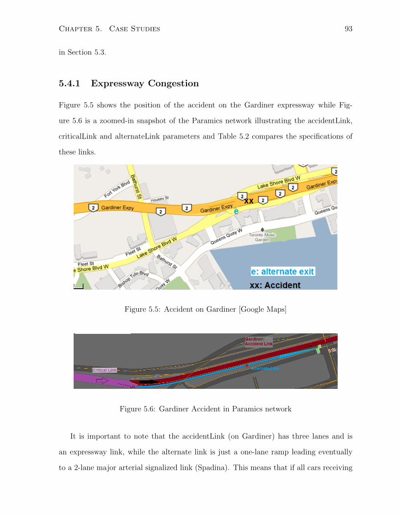
Chapter 5. Case Studies 93
in Section 5.3.
5.4.1 Expressway Congestion
Figure 5.5 shows the position of the accident on the Gardiner expressway while Fig-
ure 5.6 is a zoomed-in snapshot of the Paramics network illustrating the accidentLink,
criticalLink and alternateLink parameters and Table 5.2 compares the specifications of
these links.
Figure 5.5: Accident on Gardiner [Google Maps]
Figure 5.6: Gardiner Accident in Paramics network
It is important to note that the accidentLink (on Gardiner) has three lanes and is
an expressway link, while the alternate link is just a one-lane ramp leading eventually
to a 2-lane major arterial signalized link (Spadina). This means that if all cars receiving

Chapter 5. Case Studies 94
Table 5.2: Comparison of the specifications of accidentLink and alternateLink
accidentLink alternateExit alternateLink
Number of Lanes 3 1 2
Width 12 m 4 m 7 m
Type of Link expressway ramp signalized major arterial
Max Speed of Link 25 m/s 14 m/s 14 m/s
the message choose to turn onto the alternate link, this may lead to more congestion
than if just a portion of the cars turn. This is why we study the effect of the compliance
factor (percentage of cars changing their route as a result of the message) on network
performance. This behavior is revealed in the results discussed below.
Results
In this section, we display the results of the various experiments run on this traffic
network, however the interpretation of the parameters and performance metrics discussed
previously inSection 5.3 is not re-stated here.
Experiment 1-1: In this experiment, we test the effect of changing the compliance
factor on the average total travel time of the cars involved in the accident and on the
average queue length on all links affected by the accident (accidentLink, criticalLink
and alternateLink). A compliance factor of zero means that OMNeT++ was not called
and thus no communication took place between the cars (omnetActive = False). We
also study the case when no accident is initiated in the network as a reference for the
improvement, i.e. in order to know how much improvement is the result of communication
between cars. Table 5.3 summarizes the parameter settings for the first experiment run.
Figure 5.7 illustrates the average queue length on all links affected by the accident
for different compliance factors. The minimum average queue length is equal to 57 cars
and it occurred at 30% diversion ratio, i.e. when only 30% of the cars complied with the

Chapter 5. Case Studies 95
Table 5.3: Parameters of experiment 1-1
Total Accident Accident Number of Sending
Simulation Duration Location Lanes Message
Time Blocked Interval
90 minutes 15 minutes on Gardiner 2 out of 20 seconds
7:30 - 9:00 am 8:15 - 8:30 am expressway 3 lanes
Figure 5.7: Average Queue Length for different compliance factors

Chapter 5. Case Studies 96
message. The maximum average queue length is equal to 100 cars and it occured at 80%
diversion ratio, i.e. when 80% of the cars complied with the message.
Figure 5.8 illustrates the average total travel time of all cars involved in the accident
for different compliance factors. The minimum average total travel time is equal to 33.6
minutes and it occurred at 30% diversion ratio, i.e. when only 30% of the cars complied
with the message. The maximum average total travel time is equal to 40.6 minutes and
it occurred at 80% diversion ratio, i.e. when 80% of the cars complied with the message.
Figure 5.8: Average Total Travel Time for different compliance factors
Figure 5.9 is a merged graph of the previous two graphs. It is used to show that the
optimum diversion ratio in this case is 30% with respect to both metrics of average queue
length and average total travel time. It also shows that the worst diversion ratio is the
same and is equal to 80%. This result is expected since the accident is generated here on

Chapter 5. Case Studies 97
an expressway link of three lanes and the alternate exit is a ramp of just one lane leading
eventually to a 2-lane major arterial signalized link (Spadina). This means that there is
a trade-off between travelling on the accident link while waiting for the accident to clear
and turning onto a narrower alternate link. The more cars comply with the message by
turning onto the alternate link, the more the congestion on this link, while the fewer the
cars that comply with the message, the more the congestion on the accident link. In this
situation, the best diversion ratio is shown to be 30%.
Figure 5.9: Optimal Diversion Ratio
Figure 5.10 is a bar chart that compares the average total travel time in four different
cases. It is clear from the chart that communication between cars improved the average
total travel time in the case when the diversion percentage was 30%, however when the
diversion percentage was at its worst (80%), communication between cars led to a result
very similar to the case with no communication. Therefore, we conclude that in almost
all cases, communication between cars leads to an improvement in network performance.

Chapter 5. Case Studies 98
Figure 5.10: Bar Chart of average total travel time in 4 different cases.
Lastly, Figure 5.11 shows a comparison between the average total travel time of all
cars in the network and of only those cars involved in the accident. This is also compared
to the average total travel time of all “tagged” cars travelling on the isolated Gardiner
corridor, but in a case with no accident. The graph shows clearly that averaging over the
whole network gives a nearly constant value in all cases of accident and communication.
This is because the portion of the network affected by the accident is very small relative
to the whole network as shown previously in Figure 5.3. However, the average total
travel time of all cars in the network is much less than the average total travel time of
the cars travelling on the isolated corridor in the case with no accident. This is because
the isolated corridor is normally congested even when no accident is simulated in the
network.
Experiment 1-2: In this experiment, we test the impact of the frequency of broad-
casting the message, or in other words the sending time interval (when calling OM-
NeT++), on the number of cars successfully receiving the message and on the total CPU

Chapter 5. Case Studies 99
Figure 5.11: Comparison with average total travel time over whole network

Chapter 5. Case Studies 100
time elapsed, which represents in real life the impact on the wireless network. We fixed
the compliance factor in this experiment to 100%, because the optimum compliance fac-
tor can differ when the number of cars receiving the message changes. Therefore, we
assume that all cars receiving the message comply with it and change their route. We
also count each car only once, so if a car receives the same message more than once, only
one received message is counted. Table 5.4 summarizes the parameter settings for the
second experiment run.
Table 5.4: Parameters of experiment 1-2
Total Accident Accident Number of Compliance
Simulation Duration Location Lanes Factor
Time Blocked
90 minutes 15 minutes on Gardiner 2 out of 100%
7:30 - 9:00 am 8:15 - 8:30 am expressway 3 lanes
Figure 5.12 shows the results of this experiment. It is clear that the number of mes-
sages received decreases as the sending message interval decreases, however the decrease
rate increases as the sending message interval is widened. Therefore, in this scenario
there is no need to refine the sending message interval to a few seconds, because the
number of messages received is almost constant as long as the sending interval is less
that 45 minutes. On the other hand, the elapsed CPU time decreases exponentially as
the sending interval increases. This exponential decrease means that when the sending
interval is too short, the CPU time is too long (1.5 hours) and decreases sharply at first,
then as the sending interval increases above a minute, the CPU time almost saturates at
20 minutes. This graph shows that a sending time interval of 45 seconds is an optimum
value, since the number of messages received is almost maximum while the elapsed CPU
time is close to its minimum value.

Chapter 5. Case Studies 101
Figure 5.12: Effect of sending time interval on number of messages received and on total
CPU time elapsed.
5.4.2 Surface Street Accident
Figure 5.13 shows the position of the accident on Front St W, while Figure 5.14 is a
zoomed-in snapshot of the Paramics network illustrating the accidentLink, criticalLink
and alternateLink parameters and Table 5.5 compares the specifications of these links.
Table 5.5: Comparison of the specifications of accidentLink and alternateLink
accidentLink alternateLink-4 alternateLink-5
Number of Lanes 2 2 3
Width 7 m 7 m 10.5 m
Type of Link minor arterial collector road minor arterial
Max Speed of Link 14 m/s 11 m/s 14 m/s
The nature of this accident scenario is quite different from the scenario discussed
in Section 5.4.1. First, there are three entry links onto the accident link and therefore

Chapter 5. Case Studies 102
Figure 5.13: Accident on Front St. W [Google Maps]
Figure 5.14: Surface Street Accident on Paramics network

Chapter 5. Case Studies 103
there are three critical links and an alternate exit from each critical link as shown in
Figure 5.14. Second, the alternate links have similar or better properties than the accident
link as shown in Table 5.5 and thus, the more cars are diverted, the better the network
performance. This is reflected below in many of the results.
Results
In this section, we display the results of the various experiments run on this traffic net-
work, however the interpretation of the parameters and performance metrics discussed
previously in Section 5.3 is not re-stated here.
Experiment 2-1: In this experiment, we test the effect of changing the compliance fac-
tor on the average total travel time of the cars involved in the accident and the average
queue length on all links affected by the accident (accidentLink, criticalLink and alter-
nateLink). A compliance factor of zero means that OMNeT++ was not called and thus
no communication took place between the cars (omnetActive = False). We also study
the case when no accident is initiated in the network as a reference for the improvement,
i.e. in order to know how much improvement results from the communication between
cars. Table 5.6 summarizes the parameter settings for the first experiment run of this
accident scenario.
Table 5.6: Parameters of experiment 2-1
Total Accident Accident Number of Sending
Simulation Duration Location Lanes Message
Time Blocked Interval
45 minutes 15 minutes on Front St W 2 out of 5 seconds
7:30 - 8:15 am 7:45 - 8:00 am (surface street) 2 lanes
Figure 5.15 illustrates the average queue length on all links affected by the accident
for different compliance factors. The minimum average queue length is equal to 35 cars

Chapter 5. Case Studies 104
Figure 5.15: Average Queue Length for different compliance factors
and it occurred at 80% diversion ratio, i.e. when 80% of the cars complied with the
message. The maximum average queue length is equal to 56 cars and it occurred at 20%
diversion ratio, i.e. when only 20% of the cars complied with the message.
Figure 5.16 illustrates the average total travel time of all cars involved in the accident
for different compliance factors. The minimum average total travel time is equal to 9.2
minutes and it occurred at 80% diversion ratio, i.e. when 80% of the cars complied
with the message. The maximum average total travel time is equal to 15.1 minutes and
it occurred at 20% diversion ratio, i.e. when only 20% of the cars complied with the
message.
Figure 5.17 is a merged graph of the previous two graphs. It is used to show that
the optimum diversion ratio in this case is 80% with respect to both metrics of average
queue length and average total travel time. It also shows that the worst diversion ratio
is the same and is equal to 20%. This result is expected since the accident is generated
here on a minor arterial and the alternate links are wider than or similar to the accident

Chapter 5. Case Studies 105
Figure 5.16: Average Total Travel Time for different compliance factors
link. Therefore, the higher the diversion percentage, the better the performance of the
network.
Figure 5.18 is a bar chart that compares the average total travel time in four different
cases. It is clear from the chart that communication between cars improved the aver-
age total travel time in the case when the diversion percentage was 80%, however when
the diversion percentage was at its worst (20%), communication between cars led to a
result very similar to the case with no communication. Therefore, we conclude that com-
munication between cars led to a significant improvement in the network performance.
However, if only a few cars comply with the message, then a case with no communication
is better.
Lastly, Figure 5.19 shows a comparison between the average total travel time of all
cars in the network and of those cars involved in the accident. It is also compared to the
average total travel time of all “tagged” cars travelling on Front St and BlueJays way,
but in a case with no accident. The graph shows clearly that averaging over the whole

Chapter 5. Case Studies 106
Figure 5.17: Optimal Diversion Ratio
Figure 5.18: Bar Chart of average total travel time in 4 different cases.

Chapter 5. Case Studies 107
Figure 5.19: Comparison with average total travel time over whole network
network gives a nearly constant value in all cases of accident and communication. This
is because the portion of the network affected by the accident is very small relative to
the whole network as shown previously in Figure 5.3. Moreover, the average total travel
time of all cars in the network is almost equal to the average total travel time of cars
travelling on Front St and BlueJays way in the case with no accident.
Experiment 2-2: In this experiment, we test the impact of the frequency of broad-
casting the message, or in other words the sending time interval (when calling OM-
NeT++), on the percentage of cars receiving the message and on the total elapsed CPU
time, which represents in real life the impact on the wireless network. We fixed the com-
pliance factor in this experiment to 100% because the optimum compliance factor can
differ when the number of cars receiving the message changes. Therefore, we assume that
all cars receiving the message comply with it and change their route. We also count each
car only once, so if a car receives the same message more than once, only one received
message is counted. Table 5.7 summarizes the parameter settings for this experiment

Chapter 5. Case Studies 108
run.
Table 5.7: Parameters of experiment 2-2
Total Accident Accident Number of Compliance
Simulation Duration Location Lanes Factor
Time Blocked
45 minutes 15 minutes on Front St W 2 out of 100%
7:30 - 8:15 am 7:45 - 8:00 am (surface street) 2 lanes
Figure 5.20 shows the results of this experiment. It is clear that the percentage of
cars receiving the message decreases linearly as the sending message interval decreases.
Therefore, in this scenario it is essential to refine the sending message interval to a
few seconds, in order to make most of the cars aware of the accident and avoid the
link. Moreover, although the elapsed CPU time decreases exponentially as the sending
interval increases, the worst elapsed CPU time is less than 30 minutes which means that
the impact is very low. To conclude, this graph shows that the shorter the sending time
interval, the more messages received and thus the better the network performance. At
the same time, the elapsed CPU time is managable.

Chapter 5. Case Studies 109
Figure 5.20: Effect of sending time interval on number of messages received and on total
CPU time elapsed.

Chapter 6
Conclusions and Future
Recommendations
6.1 Summary
Vehicular communication systems enable the cooperation of vehicles traveling on roads so
that they can exchange information about accidents, traffic jams or other safety warnings
and thus enhance the overall traffic flow. These vehicular systems involve communication
between vehicles and roadside units and are developed as part of Intelligent Transporta-
tion Systems (ITS). Many ITS institutions in Europe [1] and North America [19] are
investigating the applicability of vehicular communications and are seeking to implement
these applications in real systems. Even car manufacturers and communication corpora-
tions are greatly interested in this field: for instance, Toyota and other car manufacturers
are installing Dedicated Short Range Communication (DSRC) On Board Units (OBU) in
newly developed cars to allow car-to-car and car-to-infrastructure communications [10].
Although there is ongoing interest in vehicular communication systems, there is very
little work being done to provide dedicated simulators for these types of interdisciplinary
systems. In other words, there is urgency in building simulation platforms that are capa-
110

Chapter 6. Conclusions and Future Recommendations 111
ble of testing the behavior of wireless communications in vehicular environments, so that
they can capture the finest detail of both worlds, the transportation and communication
disciplines.
In this thesis, we present a platform that combines the capabilities of a transporta-
tion network simulator and of a communication network simulator. We have chosen to
integrate two existing simulators rather than building our own combined simulator from
scratch, in order to be able to benefit from existing expertise in each field. Our micro-
scopic traffic network simulator, Paramics, and our communication network simulation
platform, OMNeT++, were chosen after extensive research.
We have designed two independent systems, an offline open loop system and an
online closed loop system. In offline mode, we extract mobility traces from Paramics and
import them into OMNeT++ to allow the latter to simulate communications between
cars moving according to a Car Following Model (from Paramics). Whereas this open
loop coupling method cannot be used to investigate applications where the information
sent to cars contains traffic content, instead it is used to design and study the performance
of entertainment applications such as vehicular internet access. As an alternative, the
online mode allows the two simulators to exchange information simultaneously in a closed
loop manner and hence is capable of testing more sophisticated applications such as traffic
congestion avoidance applications. To elaborate, the online mode allows the results of
the wireless network to be fed back to the traffic network, thereby affecting the routing
decisions of cars, which means that various traffic and ITS applications can be modeled
and tested in this mode.
6.2 Future Work
Section 6.2.1 suggests some future modifications to the current implementation of the
platform in order to adapt it to several applications. Section 6.2.2 then suggests several

Chapter 6. Conclusions and Future Recommendations 112
important ITS applications that can benefit from combining Paramics with OMNeT++.
6.2.1 Modifications
In addition to the modifications stated in Section 4.4.4, we suggest here some further
adjustments.
• Include more details on data transferred between two simulators:
Currently, the data sent from Paramics to OMNeT++ is restricted to the minimum
possible data that allows OMNeT++ to replicate Paramics (car-positions). In
future work, it may be desirable to include more data such as the type of car
(heavy vehicle, truck, bus, car, etc..) in a freight-related application. These data
can be simply included using the current plugin by adding a line that specifies the
information that needs to be sent.
• Include different message types and different behavior:
In future work, different message types could be exchanged between cars in the
network, each modeling a certain behavior. Moreover, since the messages are en-
coded by integers, the integer representing the message could be chosen to define
its priority. For example, 1 = emergency, 2 = normal accident, 3 = good flow and
so on.
• Test Different wireless protocols:
Changing the underlying wireless interface that represents a car might of interest
to future users of this platform. For example, a Bluetooth interface could be added
for some cars while leaving other cars with just the Wi-Fi interface. This can be
done easily by specifying a penetration ratio that represents the cars that have an
extra Bluetooth interface and by modeling these cars differently in the OMNeT++
simulation.

Chapter 6. Conclusions and Future Recommendations 113
• Different transportation networks with various scenarios:
Also, the transportation network under test can be changed and the basic plugins
that link Paramics and OMNeT++ can still be used. However, additional code has
to be added according to the new network topology and also to model the desired
scenario. Refer to Section 4.4.2 for more details.
6.2.2 Applications
Examples of ITS applications that can benefit greatly from the proposed simulator com-
bining Paramics with OMNeT++ include:
• Evacuation Plan: Paramics would simulate traffic conditions and OMNeT++ would
simulate the sending of messages to the targets of the evacuation plan, according
to the proposed protocol.
• Adaptive signal control application: Paramics would handle adaptive control logic
through a coded plugin and OMNeT++ would be responsible for communication
between signals at different intersections. It could also send the coordinated data
to a central server which would run optimization algorithms and help transmit the
signals, possibly through a learning process between cars and signals.
• Automatic Incident Detection (AID): The combined simulator could be used to
study the effectiveness of proposed AID techniques.

Bibliography
[1] The car-to-car communication consortium. http://www.car-2-car.org/.
[2] CORSIM. http://mctrans.ce.ufl.edu/featured/tsis/Version5/corsim.htm.
[3] Los Alamos National Laboratory (LANL). http://www.lanl.gov/.
[4] MITSIMLab. http://mit.edu/its/mitsimlab.html.
[5] Quadstone Paramics. http://www.paramics-online.com/.
[6] QualNet. http://www.qualnet.com/products/qualnet/.
[7] SWANS. http://jist.ece.cornell.edu/.
[8] The Network Simulator ns-2. http://www.isi.edu/nsnam/ns/.
[9] Topologically integrated geographic encoding and referencing system (TIGER).
http://www.census.gov/geo/www/tiger/.
[10] Toyota develops onboard DSRC unit. http://social.telematicsupdate.com/
content/toyota-develops-onboard-dsrc-unit.
[11] TRANSIMS. http://www.transims-opensource.net/.
[12] Hazem Ahmed, Mohamed EL-Darieby, Baher Abdulhai, and Yasser Morgan.
Bluetooth- and Wi-Fi-based mesh network platform for traffic monitoring. In Trans-
portation Research Board Annual Meeting, pages 192–205, January 2008.
114

Bibliography 115
[13] Aruna Balasubramanian, Ratul Mahajan, Arun Venkataramani, Brian Neil Levine,
and John Zahorjan. Interactive Wi-Fi connectivity for moving vehicles. In Proc.
ACM SIGCOMM Conf. on Data Communication, volume 38, pages 427–438, 2008.
[14] Christian Bettstetter. Smooth is better than sharp: A random mobility model for
simulation of wireless networks. In Proc. Int. Wkshp. on Modeling, Analysis, and
Simulation of Wireless and Mobile Systems, pages 19–27, 2001.
[15] Luciano Bononi, Marco Di Felice, Marco Bertini, and Emidio Croci. Parallel and
distributed simulation of wireless vehicular ad hoc networks. In Proc. of the 9th
ACM International Symposium on Modeling Analysis and Simulation of Wireless
and Mobile Systems, pages 28–35, 2006.
[16] P. Brenner. A technical tutorial on the IEEE 802.11 protocol. In BreezeCom Wireless
Communications, 1992.
[17] Vladimir Bychkovsky, Bret Hull, Allen K. Miu, Hari Balakrishnan, and Samuel
Madden. A Measurement Study of Vehicular Internet Access Using In Situ Wi-
Fi Networks. In Proc. Int. Conf. Mobile Computing and Networking, pages 50–61,
September 2006.
[18] David R. Choffnes and Fabian E. Bustamante. An integrated mobility and traffic
model for vehicular wireless networks. In VANET ’05: Proceedings of the 2nd ACM
International Workshop on Vehicular Ad Hoc Networks, pages 69–78, 2005.
[19] RITA Research And Innovative Technology Adminstration. http://www.its.dot.
gov/index.htm.
[20] Bhavyesh Divecha, Ajith Abraham, Crina Grosan, and Sugata Sanyal. Impact of
node mobility on MANET routing protocols models. Journal of Digital Information
Management, 5(1):19–24, 2007.

Bibliography 116
[21] Stephan Eichler. Performance evaluation of the IEEE 802.11p WAVE communica-
tion standard. In Proceedings of the 1st IEEE International Symposium on Wireless
Vehicular Communications WiVeC, pages 2199–2203, October 2007.
[22] E. Ferro and F. Potorti. Bluetooth and Wi-Fi wireless protocols: a survey and a
comparison. IEEE J. Wireless Communications, 12:12–26, February 2005.
[23] C. Gorgorin, V. Gradinescu, R. Diaconescu, V. Cristea, and L. Ifode. An Integrated
Vehicular and Network Simulator for Vehicular Ad-Hoc Networks. In Proc. European
Simulation and Modelling Conference (ESM), 2006.
[24] Bret Hull, Vladimir Bychkovsky, Yang Zhang, Kevin Chen, Michel Goraczko, Allen
Miu, Eugene Shih, Hari Balakrishnan, and Samuel Madden. CarTel: a distributed
mobile sensor computing system. In Proc. Int. Conf. Embedded Networked Sensor
Systems, pages 125–138, 2006.
[25] INET framework. http://www.omnetpp.org/doc/INET/neddoc/index.html.
[26] RITA Research And Innovative Technology Adminstration. http://www.
itsoverview.its.dot.gov/.
[27] William T. Kasch, Jon R. Ward, and Julia Andrusenko. Wireless network modeling
and simulation tools for designers and developers. IEEE Communications Magazine,
47(3):120–127, 2009.
[28] Christian Lochert, Andreas Barthels, Alfonso Cervantes, Martin Mauve, and Murat
Caliskan. Multiple simulator interlinking environment for IVC. In VANET ’05:
Proceedings of the 2nd ACM International Workshop on Vehicular Ad Hoc Networks,
pages 87–88, 2005.
[29] Rahul Mangharam, Daniel S. Weller, Daniel D. Stancil, Ragunathan Rajkumar, and
Jayendra S. Parikh. GrooveSim: A topography-accurate simulator for geographic

Bibliography 117
routing in vehicular networks. In Proceedings of the 2nd ACM International Work-
shop on Vehicular Ad Hoc Networks, pages 59–68, 2005.
[30] Gustavo Marfia, Giovanni Pau, Enzo De Sena, Eugenio Giordano, and Mario Gerla.
Evaluating vehicle network strategies for downtown Portland: opportunistic infras-
tructure and the importance of realistic mobility models. In MobiOpp ’07: Proceed-
ings of the 1st International MobiSys Workshop on Mobile Opportunistic Network-
ing, pages 47–51, 2007.
[31] Liam McNamara, Cecilia Mascolo, and Licia Capra. Content source selection in
Bluetooth networks. In MOBIQUITOUS ’07: Proceedings of the 2007 Fourth Annual
International Conference on Mobile and Ubiquitous Systems: Networking&Services
(MobiQuitous), pages 1–8, 2007.
[32] Mobility framework. http://mobility-fw.sourceforge.net/.
[33] V. Navda, A. Kashyap, and S. R. Das. Design and evaluation of iMesh: an
infrastructure-mode wireless mesh network. In WoWMoM ’05: Proc. Sixth IEEE
International Symposium on World of Wireless Mobile and Multimedia Networks,
pages 164–170, 2005.
[34] Vishnu Navda, Anand Prabhu Subramanian, Kannan Dhanasekaran, Andreas
Timm-Giel, and Samir Das. MobiSteer: using steerable beam directional antenna
for vehicular network access. In MobiSys ’07: Proc. Int. Conf. Mobile Systems,
Applications And Services, pages 192–205, 2007.
[35] US Department of Transportation. Traffic Control Systems Handbook. Tech-
nical report, Fedral Highway Adminstration, 2005. http://ops.fhwa.dot.gov/
publications/fhwahop06006/chapter_4.htm.
[36] OMNeT++ community site. http://www.omnetpp.org.

Bibliography 118
[37] Jorg Ott and Dirk Kutscher. A disconnection-tolerant transport for drive-thru inter-
net environments. In Proc. Int. Conf. Computer Communications, pages 1849–1862,
March 2005.
[38] Michal Piorkowski, Maxim Raya, Ada L. Lugo, Panos Papadimitratos, Matthias
Grossglauser, and Jean-Pierre Hubaux. TraNS: Realistic joint traffic and network
simulator for VANETs. ACM SIGMOBILE Mobile Computing and Communications
Review, 2007.
[39] Nedal T. Ratrout and Syed Masiur Rahman. A comparative analysis of currently
used microscopic and macroscopic traffic simulation software. The Arabian Journal
for Science and Engineering, 34(1B):121–133, 2009.
[40] Devan Bing Rehunathan, Boon-Chong Seet, and Trung-Tuan Luong. Federating
of MITSIMLab and ns-2 for realistic vehicular network simulation. In Mobility ’07:
Proceedings of the 4th International Conference on Mobile Technology, Applications,
and Systems and the 1st International Symposium on Computer Human Interaction
in Mobile Technology, pages 62–67, 2007.
[41] B. Schunemann, K. Massow, and I. Radusch. A novel approach for realistic emu-
lation of Vehicle-2-X communication applications. In Proc. IEEE Conf. Vehicular
Technology Conference, pages 2709–2713, 2008.
[42] Christoph Sommer, Zheng Yao, Reinhard German, and Falko Dressler. On the Need
for Bidirectional Coupling of Road Traffic Microsimulation and Network Simulation.
In 9th ACM International Symposium on Mobile Ad Hoc Networking and Computing
(ACM Mobihoc 2008): 1st ACM International Workshop on Mobility Models for
Networking Research (ACM MobilityModels 2008), pages 41–48, May 2008.
[43] SUMO Simulation of Urban MObility. http://sourceforge.net/apps/
mediawiki/sumo/index.php?title=Main_Page.

Bibliography 119
[44] SUMO Simulation of Urban MObility FAQ. http://sourceforge.net/apps/
mediawiki/sumo/index.php?title=FAQ.
[45] Philip John Tarnoff, Darcy M Bullock, Stanley E Young, James Wasson, Nicholas
Ganig, and James R Sturdevant. Continuing evolution of travel time data infor-
mation collection and processing. In Transportation Research Board 88th Annual
Meeting, 2009.
[46] The Diebold Institute for Public Policy Studies, Inc. Transportation Infostructures:
The Development of Intelligent Transportation Systems. Praeger, 1995.
[47] Andras Varga and Rudolf Hornig. An overview of the OMNeT++ simulation en-
vironment. In Simutools ’08: Proceedings of the 1st International Conference on
Simulation Tools and Techniques for Communications, Networks and Systems &
Workshops, pages 1–10, 2008.
[48] Axl Wegener, Micha lPiorkowski, Maxim Raya, Horst Hellbruck, Stefan Fischer, and
Jean-Pierre Hubaux. Traci: an interface for coupling road traffic and network sim-
ulators. In CNS ’08: Proceedings of the 11th Communications and Networking
Simulation Symposium, pages 155–163, 2008.
[49] Huaying Xu and Matthew Barth. A transmission-interval and power-level mod-
ulation methodology for optimizing inter-vehicle communications. In VANET ’04:
Proceedings of the 1st ACM International Workshop on Vehicular Ad Hoc Networks,
pages 97–98, 2004.
[50] Yi Yang and Rajive Bagrodia. Evaluation of VANET-based advanced intelligent
transportation systems. In VANET ’09: Proceedings of the Sixth ACM International
Workshop on VehiculAr InterNETworking, pages 3–12, 2009.