66 hf-praxis 7/2018

RF & Wireless

with a combination of available components, implementation technologies, regulatory cons-traints, requirements from the system, and signal processing.

Theory of OperationThe project in this example, Pulse_Doppler_Radar_System.emp, illustrates key models and simulation capabilities available for practical radar design. The project and resulting measure-ments highlight how to configure a pulse-Doppler (PD) radar and set up the simulation to obtain the metrics of interest for radar development. The entire PD radar system project includes a linear FM (LFM) chirp signal

generator, RF transmitter, anten-nas, clutter, RF receiver, moving target detector (MTD), constant false alarm rate (CFAR) proces-sor, and signal detector for simu-lation purposes.

PD radars produce velocity data by reflecting a microwave signal from a given target and analy-zing how the frequency of the returned signal has shifted due to the object’s motion. This variation in frequency provi-des the radial component of a target’s velocity relative to the radar. The radar determines the frequency shift by measuring the phase change that occurs in the electromagnetic (EM) pulse over a series of pulses. By mea-

suring the Doppler rate, the radar is able to determine the relative velocity of all objects returning echoes to the radar system, including planes, vehicles, and ground features.

As the reflector (target) moves between each transmit pulse, the returned signal has a phase diffe-rence or phase shift from pulse to pulse. This causes the reflector to produce Doppler modulation on the reflected signal.

System SetupThe main radar system diagram in Figure 1 includes the fol-lowing building blocks: linear chirp source, RF transmitter and

This application example show-cases how NI AWR Design Envi-ronment, specifically Visual System Simulator (VSS) system simulation software, enables radar system architects and RF component manufacturers to design, validate, and prototype a radar system. This integrated platform provides a path for digi-tal, RF, and system engineers to collaborate on complex radar system design.

Modern radar systems are com-plex and depend heavily on advanced signal processing algo-rithms to improve their detec-tion performance. At the same time, the radio front end must meet challenging specifications

An Integrated Framework for Complex Radar System Design

Figure 1: VSS main radar system diagram showing linear chirp source, RF transmitter and receiver links, target and propagation model, and receiver baseband signal processing blocks

hf-praxis 7/2018 67

RF & Wireless

receiver, and target and propa-gation models, as well as recei-ver baseband signal processing blocks, including moving tar-get indicator (MTI), MTD, and CFAR. User-defined parame-ters specifying the gain, band-

width, and carrier frequency of both the transmitter and receiver sub-blocks can be set to values based on test specifications. A detailed look at the individual components explains how this PD radar works.

The linear chirp source (first block to the far left of the system diagram) generates a linear FM chirp signal, also known as a PD signal. The linear chirp pulse source consists of basic parame-ters that can be configured accor-

ding to user specifications, such as pulse repetition frequency (PRF), pulse duty cycle, start/stop frequency, and sampling frequency. The pulse repetition interval (PRI) denotes the time difference between the starts of

Figure 2. Control parameters defining the linear chirp generator output signal

Figure 3. Components defining the RF transmitter subcircuit include an oscillator (tone source generates one or more sinusoidal tones), mixer (upconversion), filter, and amplifier

68 hf-praxis 7/2018

RF & Wireless

two consecutive pulses, shown in Figure 2. The chirp duration (pulse on) is a function of duty cycle and PRI and is calculated as the product of the two; the duty cycle is a percentage and can take any non-negative value up to and including 100%.

During the active portion of the chirp, this block outputs a signal with instantaneous frequency that changes linearly between the start and stop frequency para-meters. These two parameters can have any valid frequency value, resulting in signals that can have either increasing or decreasing frequencies at the start of the chirp. Designers are also able to specify the ratio of rise and pulse on. This parame-ter is a percentage and can have any non-negative value up to and including 100%.

The signal power during the active portion of the chirp is set by the peak power parameter of

the linear chirp signal generator. A non-zero initial delay may be defined for the chirp pulse; this delay may take on any non-negative value and a warning is generated if this delay is grea-ter than the PRI. The center fre-quency of the chirp signal may be user defined. If left empty, it is set to the average of the start and stop frequencies. Similarly, the sampling frequency may also be user defined; if left empty, it is calculated based on the global variable “_SMPFRQ”. In this example, the chirp signal level is set to 0 dBm, PRF = 2 kHz and DUTY = 25%.

The next block in the chain, a coupled correlator block, is commonly used for pulse com-pression in radar receivers. Pulse compression is a signal proces-sing technique used to increase the range resolution, as well as the signal-to-noise ratio (SNR), by modulating the transmitted

pulse and then correlating the received signal with the trans-mitted pulse. In this example, a block performs a correlation bet-ween the signal reflected from a radar target and the transmitted signal. This requires the cou-pled correlator to buffer enough samples to accommodate a full PRI before it can process the chirp. To ensure a successful simulation of such scenarios, the sampling frequency should be carefully selected. The mini-mum value for the sampling fre-quency parameter would be the bandwidth of the radar signal (FSTART-FSTOP). If spectral measurements are desired, the sampling frequency can be set to a larger value.

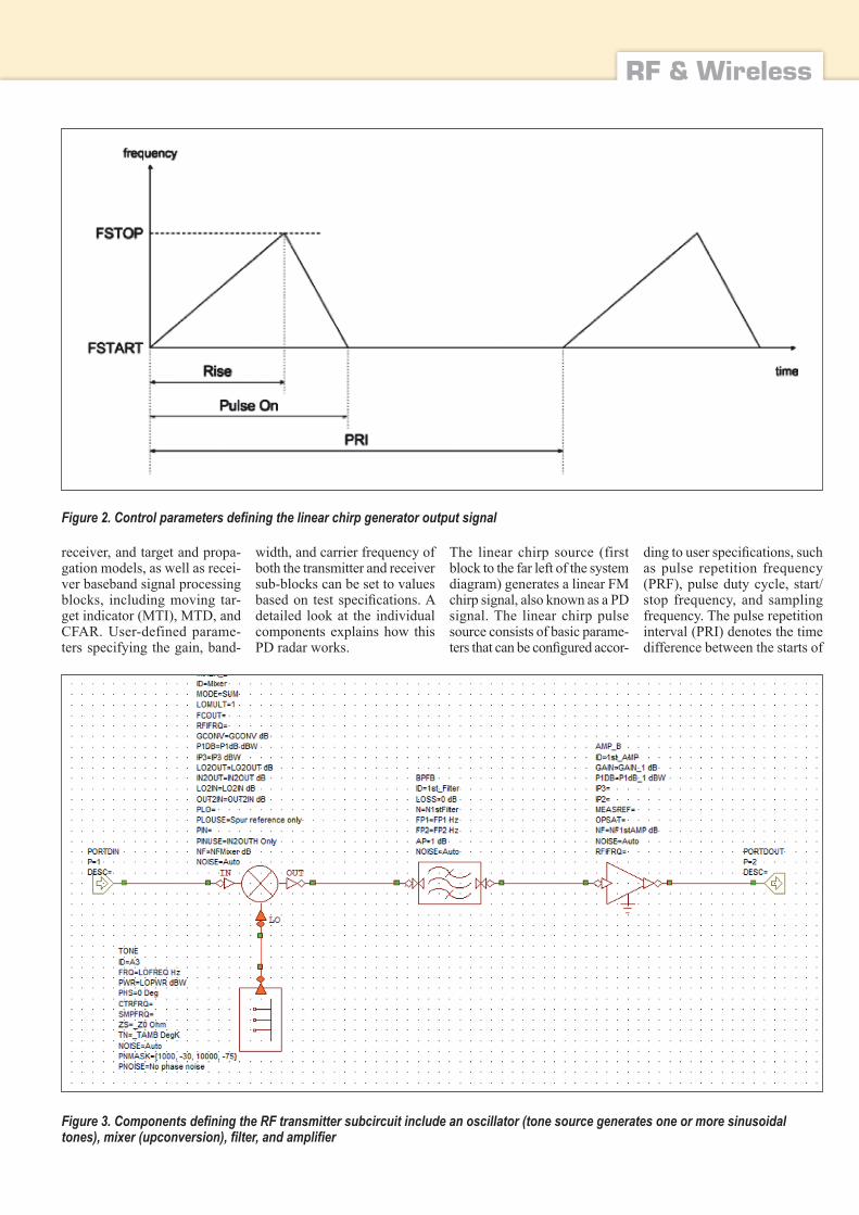
The signal next passes through the RF transmitter responsible for frequency upconversion, fil-tering, and signal amplification before being radiated through the antenna toward the target. Both

the RF transmitter and receiver subcircuits define the single stage upconverter and downcon-verter that are each composed of an oscillator, mixer, amplifier, and filter, as shown in Figure 3. Users may replace these subcir-cuits with their own particular implementations.

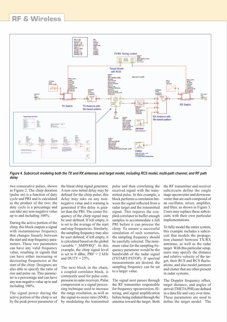
To fully model the entire system, this example includes a subcir-cuit that models the propaga-tion channel between TX/RX antennas, as well as the radar target. With this particular setup, users may specify the distance and relative velocity of the tar-get, their RCS and RCS fluctu-ations, and also model jammers and clutter that are often present in radar systems.

The Doppler frequency offset, target distance, and angles of arrival (THETA/PHI) are defined in a data file and vary over time. These parameters are used to define the target model. The

Figure 4. Subcircuit modeling both the TX and RX antennas and target model, including RCS model, multi-path channel, and RF path delay

hf-praxis 7/2018 69

RF & Wireless

clutter magnitude distribution is set to Rayleigh and the clut-ter power spectrum is formed as Weibull. The antenna radiation patterns (Figure 4) for both the transmit and receive antennas are based on filed-based data from a separate EM simula-tion, but could also be similarly modeled with measured data. The receiver filters the inco-ming reflected signal prior to amplification via a low-noise amplifier (LNA), which is then downconverted through a mixer and further filtered before input into the coupled correlator. The correlator performs correlation of the downconverted reflected signal with a coupled signal representing the input to the RF transmitter.

Radar searching, tracking, and other operations are usually car-ried out over a specified range (receive) window and defined by the difference between the radar maximum and minimum range. Reflected signals from all targets within the receive window are collected and passed through a matched filter circuitry to per-form pulse compression. The correlation processor is often

performed digitally using the fast Fourier transform (FFT).

To detect the moving object more effectively, MTD, which is based on a high-performance signal processing algorithm for PD radar, is used. A bank of Doppler filters or FFT operators cover all possible expected tar-get Doppler shifts. The output of the MTD is used for the CFAR processing. Measurements for the detection and false alarm rate are provided.

The MTI is used to remove sta-tionary objects, the MTD is used to identify the remaining moving target with the FFT size set to 64, and the CFAR performs a sliding average to ensure that the detected signal is greater than a set threshold.

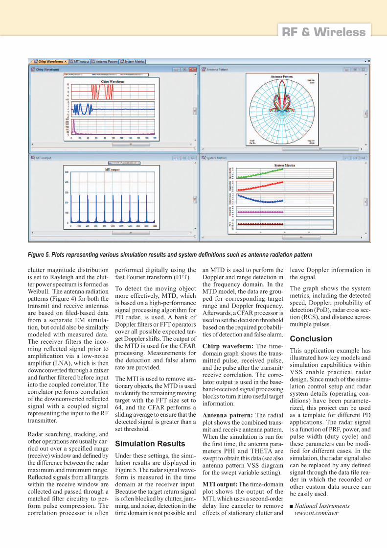
Simulation ResultsUnder these settings, the simu-lation results are displayed in Figure 5. The radar signal wave-form is measured in the time domain at the receiver input. Because the target return signal is often blocked by clutter, jam-ming, and noise, detection in the time domain is not possible and

an MTD is used to perform the Doppler and range detection in the frequency domain. In the MTD model, the data are grou-ped for corresponding target range and Doppler frequency. Afterwards, a CFAR processor is used to set the decision threshold based on the required probabili-ties of detection and false alarm.

Chirp waveform: The time-domain graph shows the trans-mitted pulse, received pulse, and the pulse after the transmit/receive correlation. The corre-lator output is used in the base-band-received signal processing blocks to turn it into useful target information.

Antenna pattern: The radial plot shows the combined trans-mit and receive antenna pattern. When the simulation is run for the first time, the antenna para-meters PHI and THETA are swept to obtain this data (see also antenna pattern VSS diagram for the swept variable setting).

MTI output: The time-domain plot shows the output of the MTI, which uses a second-order delay line canceler to remove effects of stationary clutter and

leave Doppler information in the signal.

The graph shows the system metrics, including the detected speed, Doppler, probability of detection (PoD), radar cross sec-tion (RCS), and distance across multiple pulses.

ConclusionThis application example has illustrated how key models and simulation capabilities within VSS enable practical radar design. Since much of the simu-lation control setup and radar system details (operating con-ditions) have been paramete-rized, this project can be used as a template for different PD applications. The radar signal is a function of PRF, power, and pulse width (duty cycle) and these parameters can be modi-fied for different cases. In the simulation, the radar signal also can be replaced by any defined signal through the data file rea-der in which the recorded or other custom data source can be easily used.

■  National Instruments www.ni.com/awr

Figure 5. Plots representing various simulation results and system definitions such as antenna radiation pattern