An Information Potential Approach for Tracking and...

An Information Potential Approach for Tracking andSurveilling Multiple Moving Targets using Mobile Sensor

Agents

W. Lu§, G. Zhang§, S. Ferrari§, R. Fierro†, and I. Palunko†

§Laboratory for Intelligent Systems and Control (LISC), Department of MechanicalEngineering and Materials Science, Duke University, Durham, NC, USA;

†Multi-Agent, Robotics, Hybrid, and Embedded Systems Laboratory Department of Electricaland Computer Engineering University of New Mexico, Albuquerque, NM, USA.

ABSTRACT

The problem of surveilling moving targets using mobile sensor agents (MSAs) is applicable to a variety offields, including environmental monitoring, security, and manufacturing. Several authors have shown that theperformance of a mobile sensor can be greatly improved by planning its motion and control strategies basedon its sensing objectives. This paper presents an information potential approach for computing the MSAs’motion plans and control inputs based on the feedback from a modified particle filter used for tracking movingtargets. The modified particle filter, as presented in this paper implements a new sampling method (basedon supporting intervals of density functions), which accounts for the latest sensor measurements and adapts,accordingly, a mixture representation of the probability density functions (PDFs) for the target motion. It isassumed that the target motion can be modeled as a semi-Markov jump process, and that the PDFs of theMarkov parameters can be updated based on real-time sensor measurements by a centralized processing unitor MSAs supervisor. Subsequently, the MSAs supervisor computes an information potential function that iscommunicated to the sensors, and used to determine their individual feedback control inputs, such that sensorswith bounded field-of-view (FOV) can follow and surveil the target over time.

Keywords: Target tracking, surveillance, mobile sensor networks, multi-agent systems, information value, po-tential field, particle filtering.

1. INTRODUCTION

The paradigm of the moving target surveillance using a network of mobile sensor agents (MSAs) is found ina variety of applications, including the monitoring of urban environments,1 tracking anomalies in merchandise,manufacturing plants,2 or information, and tracking of endangered species in a wild area.3 Modern surveillancesystems often consist of MSAs deployed to detect and track moving targets in a complex and unstructuredenvironment. A mobile sensor agent, comprised of an autonomous vehicle equipped with embedded wirelesssensors and communication devices, is often deployed to cooperatively track and surveil moving targets basedon limited information that only becomes available when the target enters a sensor’s field-of-view (FOV) orvisibility region. Typically, the objectives are to maximize tracking accuracy and reliability by means of limitedsensor resources, namely energy and communications. Thus, the MSAs’ performance can be greatly improved byplanning the sensor’s motion and control, and by taking into account the FOV geometry, the sensor dynamics,and the target measurements that become available over time.1,4–8 In particular, when the sensor’s FOV isbounded, the sensor’s position and orientation determine what targets can be measured at any given time.Therefore, the sensor path must be planned in concert with the measurement sequence.

Cell decomposition4,9 and probabilistic roadmap methods8 have been successfully developed for solving geo-metric sensor path planning problems with stationary targets, such as the treasure hunt. Visibility-based methods

Further author information: (Send correspondence to W.L.)W.L., G.Z., and S.F.: E-mail: {wenjie.lu, guoxian.zhang, sferrari}@duke.edu, Telephone: 1 919 660 5305R.F., and I.P.: E-mail: {rfierro, ipalunko}@ece.unm.edu, Telephone: 1 505 277 4125

Unmanned Systems Technology XIII, edited by Douglas W. Gage, Charles M. Shoemaker,Robert E. Karlsen, Grant R. Gerhart, Proc. of SPIE Vol. 8045, 80450T · © 2011 SPIE

CCC code: 0277-786X/11/$18 · doi: 10.1117/12.884116

Proc. of SPIE Vol. 8045 80450T-1

Downloaded from SPIE Digital Library on 27 Apr 2012 to 152.3.159.178. Terms of Use: http://spiedl.org/terms

have been proposed in.10–13 to account for the sensor’s dynamics and FOV. However, existing methods typicallyare not applicable to moving targets, and do not account for the uncertainty associated with target tracking,for example the uncertainty due to complex environmental conditions and online sensor measurements, where,tracking refers to the estimation of the state of a moving target through one or more sensors. The problems ofdata association and fusion that arise in tracking multiple targets by means of multiple sensors have receivedconsiderable attention.14–18 Typically, in these problems the target is modeled as a linear dynamic system withrandom disturbance inputs, and its state is predicted through frequent observations of its measurable output,which include additive random noise characterized by a Gaussian distribution. Kalman filter equations are thenused to optimally estimate the target state based on the sensor measurements collected over time. While thisapproach is well suited to long-range high-accuracy sensors, such as radars, and their applications, many of theunderlying assumptions are violated in MSAs, because the targets are non-cooperative and inherently random,and the sensor measurement errors are not additive and non-Gaussian. Furthermore, there is no systematicapproach for incorporating the results of the tracking algorithms and the effects of environmental and operatingconditions into the motion planning problem.

In this paper, a novel potential function method is developed for planning the sensor path and control inputsbased on the feedback provided by the target tracking algorithm. While the classical Kalman filter19 assumesthat the target dynamic and output equations are linear, and the random inputs can be modeled by a Gaussiandistribution, the extended Kalman filter (EKF)20 can be used when the system dynamics can be linearized aboutnominal values predicted by a Taylor expansion. The unscented Kalman filter (UKF)21 is based on the knowledgeof the mean and the covariance of a given function by the unscented transformation (UT) method,22 and canbe applied to compute the mean and covariance of a function up to the second order of the Taylor expansion.However, the efficiency of these filters tends to decrease as the system dynamics become highly nonlinear, as dueto increasingly stringent and complex operating and environmental conditions. Thus, a non-parametric methodbased on condensation and Monte Carlo simulation, known as particle filter, has been proposed23 for trackingmultiple targets exhibiting nonlinear dynamics and non-Gaussian random effects.

Particle filters are well suited to modern surveillance applications because they can be used to estimateBayesian models in which the hidden variables are connected by a Markov chain, over discrete time, but thetargets’ state is continuous, as in Markov motion models. In the particle filter method, a weighted set of particlesor point masses are used to represent the PDF of the target state by means of a superposition of weighted Diracdelta functions.24 At each iteration of the particle filter, particles representing possible target state are sampledfrom an importance density function.25 The weight associated with each particle is obtained from the target-statelikelihood function and the prior estimation PDF of the target state. When the effective particle size is smallerthan a predefined threshold, a re-sampling technique is implemented, as explained in.26 One disadvantage ofconventional particle-filtering techniques is that the target-state transition function is used as the importancedensity function to sample particles, without taking new observations into account.27 As a result, when the targetstate transition function is much broader than the likelihood function, few sampled particles have proper locationsand weights. An improved particle filter, the unscented particle filter (UPF) was proposed in,27 to overcome thisdifficulty, by combining UKF and the particle-filtering technique. The UKF generates a proposed distributionin which the current measurements are considered, and then the distribution is used as the importance densityto sample particles.

Another disadvantage of particle filters is that the point-mass representation provides limited informationabout the estimated PDF of the target state, and does not account for the targets’ dynamic equations. Toovercome both of these disadvantages of existing particle-filter tracking algorithms, this paper presents a newsampling method and a new representation for the approximation of the target state PDF that also accountsfor the target dynamics. In the proposed method, the target dynamics are modeled by a semi-Markov jumpprocess, and the particles are sampled based on the supporting intervals of the target-state likelihood functionand the prior estimation function of the target state. Where, the supporting interval of a distribution is definedas the 90% confidence interval.28 The weight for each particle is obtained by considering the likelihood functionand the transition function simultaneously. Then, the weighted expectation maximization (EM) algorithm isimplemented to use the sampled weighted particles to generate a normal mixture model of the distribution.Unlike the Dirac-delta representation, the normal mixture model of the target-state PDF can then be easily



combined with the target-dynamic equation. A potential field method is developed to plan the sensor motionand control such that each sensor can surveil a target, by maintaining a predefined distance between its platformand the target, such that the target remains inside the sensor’s FOV. The stability of the resulting sensor controllaw is guaranteed using Lyapunov stability theory.

This paper is organized as follows. Section 2 describes the tracking and surveillance problem formulationand assumptions. The background on the particle filter and the potential field methods is reviewed in Section3. Section 4 describes the new sampling method used in particle filter and the mixture Gaussian distributionrepresentation for the approximation of the target state PDF, as well as a modified potential field method. Thesimulations and results are shown in Section 5. Conclusions and future work are given in Section 6.

2. PROBLEM FORMULATION AND ASSUMPTIONS

The problem considered in this paper consists of determining the motion and control law of a MSA, indexed byi ∈ IS , deployed for the purpose of tracking and surveilling a moving point-mass target, indexed by j ∈ ITT , in aregion of interest (ROI) comprised of a bounded, two-dimensional Euclidian workspace W ∈ R

2. Where, IS andIT denote the index sets of the network of MSAs and targets, respectively, and it is assumed that the assignmentproblem has been resolved through multitarget-multisensor data association and assignment algorithms.29,30

The sensor has platform geometry Ai ∈ R2, and a bounded FOV Si ∈ R

2. FAi is a moving Cartesian frameembedded in Ai such that every point of Ai, and every point of Si, have fixed positions with respect to FAi .Then, using a suitable transformation, the ith sensor state Yκ

i = [xκi yκ

i xκi yκ

i ]T can be used to specify theposition and orientation of all points in Ai and Sj at tκ, with respect to a fixed inertial frame FW , embeddedin W. Where, xκ

i and yκi are the coordinates of the ith sensor in FW , and xκ

i and yκi are its linear velocities in

FW . Additionally, let vκi = [xκ

i , yκi ]T . Now, let ρij denote the geometric distance between the origin of FAi and

its nearest target j in W. Then, the objective of the ith MSA is to maintain ρij within a predefined range,

ρ0 < ρij < ρ1 (1)

while avoiding a set of known, fixed, and rigid obstacles in W, denoted by Bl, l ∈ IB . Where, IB is an obstacleindex set, and ρ0 and ρ1 are constant parameters specified by the user.

In this paper, it is assumed that the FOV of every sensor i ∈ IS is a disk Si ∈ R2 with radius r. The sensor

dynamics are assumed to be linear and time-invariant (LTI), and to be discretized with respect to time, suchthat the sensor state transition function can be written in state-space form as,

Yκ+1i = AYκ

i +

⎡⎣0

0δ

⎤⎦uκ

i , for κ = 0, 1, . . . , (2)

where, κ is the time index, δ is the time span between tκ+1 and tκ, ui ∈ R2 is the control vector, vκ

i = uκi , and,

A ≡

⎡⎢⎢⎣

1 0 δ 00 1 0 δ0 0 1 00 0 0 1

⎤⎥⎥⎦ (3)

For simplicity, the sensor geometry is assumed to only translate in W, such that the heading of the sensor ismaintained constant at all times.

The motion of target j ∈ IT is modeled as a continuous-time Markov motion process, also known as semi-Markov jump process,31 where, we say that xt is a continuous-time Markov process if for 0 ≤ t0 < · · · <tk−1 < tk < t we have Pr(xt ∈ B | xk = sk, xk−1 = sk−1, · · · , x0 = s0) = Pr(xt ∈ B | xk = sk) where Prdenotes the probability transition function, and s1, . . . , sk ∈ X are realizations of the state space X . Now, letthe random variables θk

j and vkj represent the jth target’s heading and velocity, respectively, during the time

interval Δtk = (tk+1 − tk), k = 1, 2, . . .. Then, the target motion can be modeled as a continuous-time Markovprocess with a family of random variables {xk

j , θkj , vk

j }, where xkj ∈ W is the jth target position at tk. A three-

dimensional real-valued vector function maps the family of random variables {θkj , vk

j } into the random vector



xj(t), representing the target position at every time t ∈ [t0, tf ], such that the value of the target motion processis given by,

xj(t) = vj(t)[cos θj(t) sin θj(t)]T , (4)

and, therefore, the motion of target j is a Markov process. The third component of the vector function is theidentity function. It follows that θj and vj are piece-wise constant, while xj has discontinuities at the timeinstants tk, when the target j changes its heading and velocity. In this paper, it is assumed that the instantswhen the target changes its heading are known a-priori, and all targets move at a constant speed vj = v. Also,it assumed that all time intervals are of constant length, i.e., Δtk = τ , for ∀k.

Now, let Xkj = [xk

j θkj ]T denote the jth target state at time step k. The probability transition function for

the target heading at the instant tk of a discontinuity, is defined as,

f(θk+1j | θk

j ) = N (θk+1j | μ + θk

j , σ2) (5)

where the mean of heading change μ and the variance of the heading change σ are constant parameters that areassumed known a-priori. The target heading remains constant during every time interval Δtk, The target statetransition function at every discontinuity is given by,

Xk+1i = Xk

j +

⎡⎣cos(θk

j )τvsin(θk

j )τvN (μ, σ2)

⎤⎦ , for ∀k. (6)

where τ is the known length of the time interval Δtk.

The MSA network attempts to obtain measurements of the targets’ positions once with a frequency of 1/δ(Hz), where δ < τ . Thus, if a time instant tκ, the jth target is inside the ith sensor’s FOV, then the ith MSAcan obtain a measurement of the jth target position,

zκi = xκ

j + νij ⇐⇒ xj(tκ) ∈ Si (7)

where xκj is the jth target’s position at time tκ, and νij is a white-noise error with standard deviation Σij . If

xj(tκ) �∈ Si, no measurements are returned to the ith sensor.

3. BACKGROUND

3.1 Particle Filter Methods

The particle filter technique is a recursive model estimation technique based on sequential Monte Carlo. It isapplicable to nonlinear system dynamics, with non-Gaussian random inputs. Moreover, because of their recursivenature, particle filters are easily applicable to online data processing and estimation. The main idea of particlefilters is to represent the PDF functions with properly weighted and relocated point-mass, known as particles.These particles are sampled from an importance density which is crucial to the particle filter algorithm. Let{xκ

j,p, wκj,p}N

p=1 denote the weighted particles that are used to approximate the posterior PDF f(xκj | Zκ

j ) for thejth target at tκ, where Zκ

j = {z0j , . . . , z

κj } denotes the set of all measurements obtained by sensor i, from target

j, up to tκ. Then, the posterior probability density function of the target state, given the measurement at tκcan be modeled as,

f(xκj | Zκ

j ) =N∑

p=1

wκj,pδ(x

κj,p),

N∑p=1

wκj,p = 1 (8)

where wκj,p is non-negative and δ is the Dirac delta function.23 Although different particle filter techniques have

been proposed,25 the techniques always consist of the recursive propagation of the particles and the particleweights. In each iteration, the particles xκ

j,p are sampled from the importance density q(x). Then, weight wkj,p

is updated for each particle by

wκj,p ∝

p(xκj,p)

q(xκj,p)

(9)



where p(xκj,p) ∝ f(xκ

j,p | Zκj ). Additionally, the weights are normalized at the end of each iteration.

The target state transition function is used as the importance density function. Thus, the sampled particlescan not fully represent the target state estimation since they are sampled without considering the new measure-ment. Another common drawback of particle filters is the degeneracy phenomenon,27 i.e., the variance of particleweights accumulates along iterations. This phenomenon indicates that a number of particles have low weightsand no contributions in approximating the probability density function f(xκ

j | zκj ) but put heavy computational

burden to the algorithm. A common way to evaluate the degeneracy phenomenon is the effective sample sizeNe,26 obtained by

Ne =1∑N

p=1(wκj,p)2

(10)

where wκj,p, p = 1, 2, . . . , N are the normalized weights. In general, a re-sampling procedure is taken when

Ne < Ns, where Ns is a predefined threshold, and is usually set as N2 . Let {xκ

j,p, wκj,p}N

p=1 denote the particleset that needs to be re-sampled, and let {xκ∗

j,p, wκ∗j,p}N

p=1 denote the particle set after re-sampling. The mainidea of this re-sampling procedure is to eliminate the particles having low weights by re-sampling {xκ∗

j,p, wκ∗j,p}N

p=1

from {xκj,p, w

κj,p}N

p=1 with the probability of p(xκ∗j,p = xκ

j,s) = wκj,s. At the end of the resampling procedure,

wκ∗j,p, p = 1, 2, . . . , N are set as 1

N . However, the resampling procedure repeats the particles with high weights anumber of times stochastically. This leads to diversity loss of particles.

In this paper, a modified particle filter approach with a new sampling method based on supporting intervalsof PDFs is proposed. The advantage of the proposed sampling method is that the latest measurement by sensorsis taken into account when particles are sampled. Moreover, a mixture Gaussian is used to represent the PDFof the target state instead of a set of properly weighted and located point-mass approximation by Dirac deltafunction in order to avoid the degeneracy phenomenon.

3.2 Potential Field

The potential field method is a robot motion planning technique that uses an artificial potential function tofind the obstacle-free path in an Euclidean workspace. The geometries and positions of the obstacles andtargets are considered as sources to construct a potential function U which represents the characteristics ofthe workspace. Although different approaches have been proposed to generate the potential function based onobstacles’ geometries,32–34 typically the potential function consists of two components, the repulsive potentialUrep generated by the obstacles,35 and the attractive potential Uatt generated by the robot goal configuration,

U(q) = Uatt(q) + Urep(q) (11)

where q = [x y θ]T is the robot configuration inW, which specifies the robot’s position (x and y coordinates) andorientation (θ) with respect to FW .35 Recently, an information potential approach was developed for generatingan attractive potential based on target geometries and information value in sensor path planning problems, suchas the treasure hunt.36 Once the potential is generated, a virtual force is applied on the robot that is proportionalto the negative gradient of U , and can be implemented through a suitable control law, such that U constitutesa Lyapunov function that may be utilized to prove closed-loop stability.

For a robot with a finite platform geometry A, the potential field is generated by taking into considerationthe robot configuration space C, and the corresponding obstacles’ geometries B. A C-obstacle is defined as thesubset of C that causes collisions with at least one obstacle in W, i.e., CBl ≡ {q ∈ C | A(q)∩Bl �= ∅}, where A(q)denotes the subset of W occupied by the platform geometry A when the robot is at the configuration q. Theunion of all C-obstacles in W is referred to as the C-obstacle region. Thus, in searching for targets in W, therobotic sensor is free to rotate and translate in the free configuration space, which is defined as the complementof the C-obstacle region CB in C, i.e., Cfree = C\CB.35

Then, the repulsive potential can be represented as,

Urep(q) =

{12η( 1

ρ(q) − 1ρ0

)2 if ρ(q) ≤ ρ0

0 if ρ(q) > ρ0

(12)



where η is a scaling factor, ρ(q) is the distance between the robot and the nearest obstacle in Euclidean space,and ρ0 is a constant parameter that is chosen by the user. The attractive potential is given by,

Uatt(q) =12ερ2

goal(q) (13)

where ε is a scaling factor, and ρgoal(q) is the distance between the robot and the goal configuration. In (12) and(13), only the obstacle closest to q is considered to generate Urep(q), and the target is assumed to be a singlepoint in Cfree. This makes the potential function difficult to update when new obstacles and targets are sensedduring the path execution, because for each value of q, the potential needs to update by computing its distancefrom the closest obstacle and target.

In this paper, a modified potential function that taking the target Markov properties into account is proposedin order to shorten sensors’ traveling distance. Furthermore, when the geometric distance ρ between the sensorplatform and nearest target is smaller than ρ0, the target is treated as an obstacle, while ρ is greater than ρ1,the target is treated as a target.

4. METHODOLOGY

The methodology presented in this paper obtains a potential-field based control law for an MSA, to surveil atarget based on the tracking information provided by a modified particle filter. For simplicity, it is assumedthat the target velocity is known and constant, and the time instants at which the discontinuities take place areknown and occur at constant intervals. However, the methodology can be generalized, and these assumptionsrelaxed, by computing the probability density functions (PDFs) of all Markov parameters using the proposedparticle filter. Here, the particle filter technique is used to obtain the PDF of the target heading, and to updateit with every new measurement zκ

j over time. In the proposed method, a finite normal mixture is utilized torepresent the PDF of the target heading,

f(θ) =m∑

�=1

π�N (θ | μ�, σ2� ),

m∑�=1

π� = 1, 0 ≤ π� (14)

where f(·) is used to denote a PDF of the arguments in parenthesis, m is the number of normal components,which is assigned a user-defined upper limit M . μ� and σ� are the mean and variance for �th normal component.Prior to obtaining target measurements, the number of components is set to m = M , μ� is uniformly sampledfrom the interval [−π π], and σ� is chosen equal to a user-defined value σ0. Let zκ

j denote the measurementobtained by sensor i at tκ, as shown in (7). Then, the PDF of the jth target’s heading at tκ, based on the setZκ

j , modeled by the finite normal mixture,

f(θκj | Zκ

j ) ←m∑

�=1

πκj,�N (θκ

j | μκj,�, (σ

κj,�)

2) (15)

is updated based on the target transition probability function (5). Since the change in the target state ischaracterized by a Gaussian distribution, i.e.,

θκ+1j − θk

j ∼ N (μ, σ2) (16)

then, the distribution of θκ+1j given Zκ

j without considering zκ+1j is given by ,

θκ+1j | Zκ

j ∼ N (μ, σ2) +m∑

�=1

πκj,�N (μκ

j,�, (σκj,�)

2)

∼m∑

�=1

πκj,�(N (μ, σ2) +N (μκ

j,�, (σκj,�)

2))

∼m∑

�=1

πκj,�N (μκ

j,� + μ, (σκj,�)

2 + σ2) (17)



Thus, the PDF of the target heading at tκ+1 is given by

f(θκ+1j | Zκ

j ) =m∑

�=1

πκj,�N (θκ+1

j | μκj,� + μ, (σκ

j,�)2 + σ2) (18)

When the measurement zκ+1j is considered, Bayes’ rule is utilized to obtain f(θκ+1

j | Zκ+1j ), based on zκ+1

j

and f(θκ+1j | Zκ

j ), as follows,

f(θκ+1j | Zκ+1

j ) ← f(θκ+1j | zκ+1

j , Zκj )

=f(zκ+1

j | θκ+1j , Zκ

j )f(θκ+1j | Zκ

j )

f(zκ+1j | Zκ

j )

∝ f(zκ+1j | θκ+1

j , Zκj )f(θκ+1

j | Zκj ) (19)

where f(zκ+1j | θκ+1

j , Zκj ) can be determined from the measurement model,

f(zκ+1j | θκ+1

j , Zκj ) ≈ f(zκ+1

j | θκ+1j , xκ

j )

=1√

2π‖∑j ‖

exp (−‖zκ

j − xκj − δv

[cos(θκ+1

j )sin(θκ+1

j )

]‖2

2‖∑j ‖2

)

where∑

j is the covariance, v is the target linear velocity, xκj is the target position estimation obtained at tκ. To

evaluate equation (19), the modified particle filter is used, in which the importance density function is based onthe supporting intervals of distributions. f(zκ

j | θκ+1j , Zκ

j ) and f(θκ+1j | Zκ

j ) are both considered as distributionsof θκ+1

j . Let S denote the support interval. Let R denote the definitive range for a distribution. S of f(x) isdefined as f(x) > γ,∀x ∈ S. Let Sm

j denote the support interval of f(zκj | θκ+1

j , Zκj ) and Sp

j denote the supportinterval of f(θκ+1

j | Zκj ). Then, S = Sm

j ∪ Spj . The importance density function for sampling particles is defined

as

f(θκ+1j ) =

{1L if θκ+1

j ∈ S

0 else(20)

where

L =∫

R

g(θκ+1j )dθκ+1

j , g(θκ+1j ) =

{1 if θκ+1

j ∈ S

0 else(21)

The weight for each particle is obtained by considering the target state likelihood function and the previoustarget state estimation together simultaneously. By considering f(zκ+1

j | θκ+1j , Zκ

j ) and f(θκ+1j | Zκ

j ), the weightwκ+1

j,p for pth particle of jth target, denoted as θκ+1j,p , is set as

wκ+1j,p = f(zκ+1

j,p | θκ+1j,p , Zκ

j )f(θκ+1j,p | Zκ

j ) (22)

The weight for each particle is normalized via

wκ+1j,p =

wκ+1j,p∑N

p=1 wκ+1j,p

(23)

Then weighted EM algorithm, shown in Table 1, is adopted to obtain a normal mixture representation of thetarget heading’s PDF, using weighted particles. After the target heading is obtained, the target position isestimated based on the sensor measurement over the latest time interval, using the least square error method.

In order to maintain the desired distance ρij between sensor i and target j within the desired range (1), anew potential function is presented, such that when the distance from the sensor to the target is less than ρ0,



Table 1. Weighted EM Algorithm

Initialize∑M

�=1 πκ+1j,� N (μκ+1

j,� , σκ+1j,� ) as

∑M�=1 πκ

j,�N (μκj,�, σ

κj,�)

Iterate until∑M

�=1 πκ+1j,� N (μκ+1

j,� , σκ+1j,� ) converges

for each particle pfp,� = πκ+1

j,� N (θκ+1j,p | μκ+1

j,� , σκ+1j,� )

cluster pth particle into group Gl if fp,� ≥ fp,r �=�

endfor each group �

μκ+1j,� =

∑wκ+1

j,p θκ+1j,p∑

wκ+1j,p

, θκ+1j,p ∈ G�

σκ+1j,� =

∑wκ+1

j,p (θκ+1j,p −μκ+1

j,� )2∑wj,p

, θκ+1j,p ∈ G�

πκ+1j,� =

∑wκ+1

j,p , θκ+1j,p ∈ G�

endif πκ+1

j,� ≤ ζ

set πκ+1j,� = 0

endend

U becomes a repulsive potential, when the distance is greater than ρ1, U becomes an attractive potential, andotherwise U is zero. Let qκ

i denote the configuration of sensor i, and qκj denote the configuration of target j at

tκ. Without considering the knowledge of targets’ Markov property, the potential function for the ith sensor attime tκ would be defined as,

U(qκi ) =

⎧⎪⎨⎪⎩

12η( 1

ρ(qκj ,qκ

i ) − 1ρ0

)2, if ρ(qκj ,qκ

i ) ≤ ρ0

0, if ρ0 < ρ(qκj ,qκ

i ) < ρ1

12ξ(ρ(qκ

j ,qκi )− ρ1)2, if ρ(qκ

j ,qκi ) ≥ ρ1

(24)

and this potential field is referred as the exact potential field. In order to shorten sensors’ travelling distance, theheading of the target during next segment, denoted as θk+1, is considered when potential field is constructed.The expectation of θk+1, denoted by θk+1, is obtained via equation (5),

θjk+1

= E{θjk+1} =

m∑�=1

πκj,�θ

κj,� + μ

Then the potential field that takes knowledge of target motion into account can be established via

U(qκi ) =

⎧⎪⎨⎪⎩

12η( 1

ρ(qκj ,qκ

i ) − 1ρ0

)2, if ρ(qκj ,qκ

i ) ≤ ρ0

0, if ρ0 < ρ(qκj ,qκ

i ) < ρ1

12ξ(ρ(qκ∗,qκ

i )− ρ1)2, if ρ(qκj ,qκ

i ) ≥ ρ1

(25)

where

qκ∗ = qκj + α

[cos θk+1

j

sin θk+1j

](ρ(qκ

j ,qκi )− ρ1) (26)

where the parameter α is a constant, qκj and qκ

i are the target and the sensor configurations respectively. Thispotential field is referred as the virtual potential field, which is different from the one established by equation(24). When the distance between the sensor and the target is in predefined interval, qκ∗ = qκ

j , which indicatesthe virtual potential field converges to the exact potential field. The artificial force is provided by the negativegradient of U ,

F(qκi ) = −�U(qκ

i ), (27)



where, from (24), the force provided by the potential field is given by,

F (qκi ) =

⎧⎪⎨⎪⎩

η( 1ρ(qκ

j ,qκi ) − 1

ρ0)�ρ(qκ∗,qκ

i )ρ2(qκ∗,qκ

i ) if ρ(qκj ,qκ

i ) ≤ ρ0

0 if ρ0 < ρ(qκj ,qκ

i ) < ρ1.

−ξ(ρ(qκ∗,qκi )− ρ1)�ρ(qκ∗,qκ

i ) if ρ(qκj ,qκ

i ) ≥ ρ1

(28)

Then, similar to,37,38 the control law u defined in terms of the artificial force is,

u(qκi ) = (xκ

j − vκi ) + F (qκ

i ). (29)

The Lyapunov function

V =12(xκ

j − vκi )T (xκ

j − vκi ) + U(qκ

i ) (30)

is considered as a possible positive semidefinite candidate, in order to analyze the stability of the control law(29). From (2), (29), and (30), the time derivative of the chosen Lyapunov function is given by:

V = (xκj − vκ

i )(−vκi )− �U(qκ

i )(xκj − vκ

i )

= (xκj − vκ

i )(−(xκj − vκ

i ) + �U(qκi ))− �U(qκ

i )(xκj − vκ

i )

= −(xκj − vκ

i )T (xκj − vκ

i ) ≤ 0 (31)

Furthermore, V ≥ 0 because U(qκi ) ≥ 0. Thus, considering V ≤ 0, the system under the control law (29) is

asymptotically stable.

5. SIMULATIONS AND RESULTS

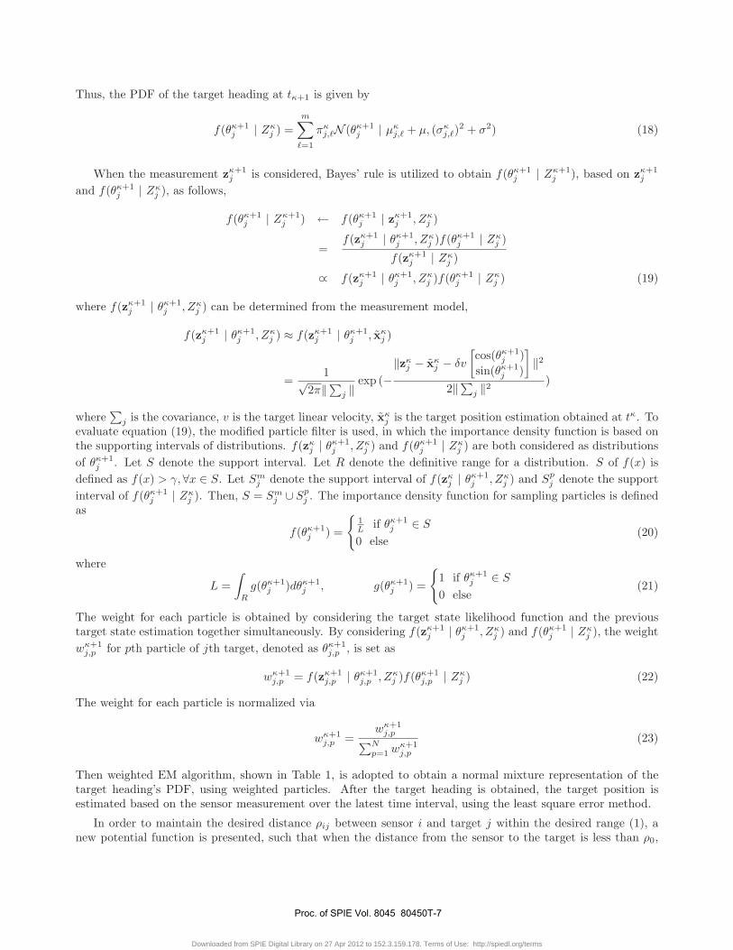
To determine the effectiveness of the proposed methodologies, simulations are run in two different scenarios. Thefirst, which is primarily used to test the modified particle filter, does not consider the geometries of the sensorand target, as they are modeled as point masses. The second scenario addresses the geometries of both sensorand target, and includes obstacles in the workspace. Scenario 1, as previously stated, models the sensor platformand the target as point masses. The workspace is defined as an obstacle free area with dimensions 50m × 50m.A single target, that changes its heading every 10 s, maneuvers the environment at a speed of 2m/s. The sensor,with an omnidirectional FOV of radius 10m, is deployed in order to track the target. The position of the targetis measured every 0.3 s by the sensor, and it is assumed that the measurements have a standard deviation, Σ =diag(0.4, 0.4). To determine the effectiveness of the modified particle filter, the estimation error of the targetheading inference is calculated. The estimation error, for a time interval, is defined as

ε = θκ − θκ (32)

where θκ is the target heading estimation, and θκ is the true value of the target heading.

The estimation error associated with the modified particle filter in the first scenario is shown Fig. 1. As seenin the plot, at the beginning of the simulation, the initial estimation of the heading varies greatly with the targetsactual heading, but converges to it quickly. The spikes denoted by k = 1 and k = 2 in the plot correspond to achange in the targets heading direction, as explained above. The estimation error grows dramatically when thetarget suddenly changes its direction. As the sensor updates its measurements, the estimation error, once again,quickly converges to zero. The simulations for the first scenario, although simple, exhibit the effectiveness of themodified particle filter in estimating the heading position of the target, and therefore the tracking abilities ofthe sensor.

The simulations of the second scenario, which consider finite target and platform geometries, also implementthe dynamics used in scenario 1. However, the workspace is expanded to 100m × 10m, and is populated withseven obstacles, modeled as convex polygons. For these simulations, the objective of the sensor is to maintainthe distance ρij , from the sensor to the target, between 3m and 4m, while avoiding the obstacles. The resultsof the simulations for scenario 2 can be found in Fig. 2, and Fig. 3 shows the path of the sensor platform, A,



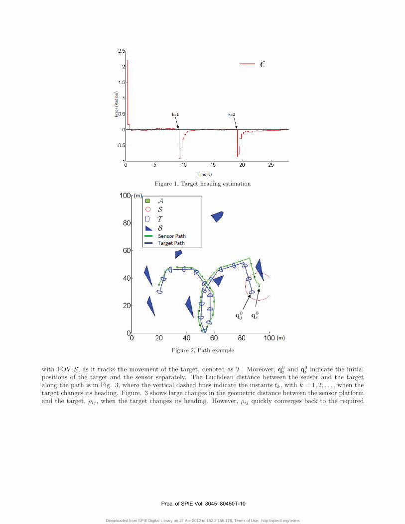
Figure 1. Target heading estimation

Figure 2. Path example

with FOV S, as it tracks the movement of the target, denoted as T . Moreover, q0j and q0

i indicate the initialpositions of the target and the sensor separately. The Euclidean distance between the sensor and the targetalong the path is in Fig. 3, where the vertical dashed lines indicate the instants tk, with k = 1, 2, . . . , when thetarget changes its heading. Figure. 3 shows large changes in the geometric distance between the sensor platformand the target, ρij , when the target changes its heading. However, ρij quickly converges back to the required



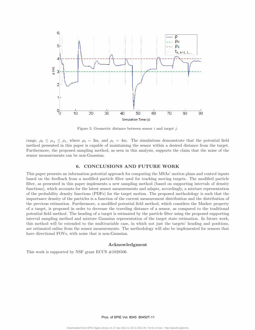
Figure 3. Geometric distance between sensor i and target j.

range, ρ0 ≤ ρij ≤ ρ1, where ρ0 = 3m, and ρ1 = 4m. The simulations demonstrate that the potential fieldmethod presented in this paper is capable of maintaining the sensor within a desired distance from the target.Furthermore, the proposed sampling method, as seen in this analysis, supports the claim that the noise of thesensor measurements can be non-Gaussian.

6. CONCLUSIONS AND FUTURE WORK

This paper presents an information potential approach for computing the MSAs’ motion plans and control inputsbased on the feedback from a modified particle filter used for tracking moving targets. The modified particlefilter, as presented in this paper implements a new sampling method (based on supporting intervals of densityfunctions), which accounts for the latest sensor measurements and adapts, accordingly, a mixture representationof the probability density functions (PDFs) for the target motion. The proposed methodology is such that theimportance density of the particles is a function of the current measurement distribution and the distribution ofthe previous estimation. Furthermore, a modified potential field method, which considers the Markov propertyof a target, is proposed in order to decrease the traveling distance of a sensor, as compared to the traditionalpotential field method. The heading of a target is estimated by the particle filter using the proposed supportinginterval sampling method and mixture Gaussian representation of the target state estimation. In future work,this method will be extended to the multivariable case, in which not just the targets’ heading and positions,are estimated online from the sensor measurements. The methodology will also be implemented for sensors thathave directional FOVs, with noise that is non-Gaussian.

Acknowledgment

This work is supported by NSF grant ECCS #1028506.



REFERENCES1. S. Ferrari, C. Cai, R. Fierro, and B. Perteet, “A multi-objective optimization approach to detecting and

tracking dynamic targets in pursuit-evasion games,” in Proc. of the 2007 American Control Conference,pp. 5316–5321, (New York, NY), 2007.

2. D. Culler, D. Estrin, and M. Srivastava, “Overview of sensor networks,” Computer 37(8), pp. 41–49, 2004.3. P. Juang, H. Oki, Y. Wang, M. Martonosi, L. Peh, and D. Rubenstein, “Energy efficient computing for

wildlife tracking: Design tradeoffs and early experiences with zebranet,” Proc. 10th International Conferenceon Architectural Support for Programming Languages and Operating Systems (ASPLOS-X) , 2002.

4. C. Cai and S. Ferrari, “Information-driven sensor path planning by approximate cell decomposition,” IEEETransactions on Systems, Man, and Cybernetics - Part B 39(3), pp. 607–625, 2009.

5. P. Cheng, G. Pappas, and V. Kumar, “Decidability of motion planning with differential contraints,” inProceedings of the 46nd IEEE International Conference on Robotics and Automation, pp. 1826–1831, (RomaItaly), 2007.

6. S. Ferrari, R. Fierro, B. Perteet, C. Cai, and K. Baumgartner, “A geometric optimization approach todetecting and intercepting dynamic targets using a mobile sensor network,” SIAM Journal on Control andOptimization 48(1), pp. 292–320, 2009.

7. K. Baumgartner and S. Ferrari, “A geometric transversal approach to anayzing track coverage in sensornetworks,” IEEE Transactions on Computers 57(8), 2008.

8. G. Zhang, S. Ferrari, and M. Qian, “Information roadmap method for robotic sensor path planning,” Journalof Intelligent and Robotic Systems 56(1-2), pp. 69–98, 2009.

9. S. Ferrari and C. Cai, “Information-driven search strategies in the board game of clue,” IEEE Transactionson Systems, Man, and Cybernetics - Part B 39(3), pp. 607–625, 2009.

10. V. Isler, C. Belta, K. Daniilidis, and G. Pappas, “Hybrid control for visibility-based pursuit-evasion games,”in Proc. of 2004 IEEE/RSJ International Conference on Intelligent Robots and Systems, pp. 1432–1437,(Sendai, Japan), 2004.

11. L. Lulu and A. Elnagar, “A comparative study between visibility-based roadmap path planning algorithms,”in IEEE/RSJ International Conference on Intelligent Robots and Systems, pp. 3263 – 3268, 2005.

12. S. Bhattacharya, R. Murrieta-Cid, and S. Hutchinson, “Optimal paths for landmark-based navigation bydifferential-drive vehicles with field-of-view constraints,” Robotics, IEEE Transactions on 23(1), pp. 47 –59,2007.

13. M. Baumann, S. Leonard, E. Croft, and J. Little, “Path planning for improved visibility using a probabilisticroad map,” Robotics, IEEE Transactions on 26(1), pp. 195 –200, 2010.

14. Y. BarShalom, X. R. Li, and T. Kirubarajan, Estimation with Applications to Tracking and Navigation:Algorithms and Software for Information Extraction, Wiley and Sons, 2001.

15. Y. BarShalom and W. D. Blair, MultitargetMultisensor Tracking: Applications and Advances, Artech House,2000.

16. Y. BarShalom and X. R. Li, MultitargetMultisensor Tracking: Principles and Techniques, YBS Publishing,1995.

17. S. S. Blackman, Multiple-Target Tracking with Radar Applications, Artech House, 1986.18. C. L. Morefiled, “Decision-directed approach to multitarget tracking,” IEEE Trans. on Automatic Con-

trol 22(3), 1977.19. G. B. G. Welch, “An introduction to the kalman filter,” tech. rep., Department of Computer Science,

University of North Carolina at Chapel Hill.



20. S. J. Julier and J. K. Uhlmann, “A new extension of the kalman filter to nonlinear systems,” Proc. AeroSense:11th Int. Symp. Aerospace/Defense Sensing, Simulation and Controls, pp. 182-197 , 1997.

21. E. Wan and R. Van Der Merwe, “The unscented kalman filter for nonlinear estimation,” in Proceedings ofthe IEEE 2000 Adaptive Systems for Signal Processing, Communications, and Control Symposium, pp. 153–158, 2000.

22. S. Julier, “The scaled unscented transformation,” in American Control Conference, 2002. Proceedings of the2002, 6, pp. 4555–4559, 2002.

23. Z. Khan, T. Balch, and F. Dellaert, “An mcmc-based particle filter for tracking multiple interacting targets,”in Computer Vision - ECCV 2004, T. Pajdla and J. Matas, eds., pp. 279–290, 2004.

24. C. Kreucher, K. Kastella, and O. Hero, “Multitarget tracking using the joint multitarget probability density,”IEEE Transactions on Aerospace and Electronic Systems 41(4), pp. 1396–1414, 2005.

25. M. Arulampalam, S. Maskell, N. Gordon, and T. Clapp, “A tutorial on particle filters for onlinenonlinear/non-gaussian bayesian tracking,” Signal Processing, IEEE Transactions on 50(2), pp. 174 –188,2002.

26. J. Carpenter, P. Clifford, and P. Fearnhead, “Improved particle filter for nonlinear problems,” in Radar,Sonar and Navigation, IEEE Proceedings, 146(1), pp. 2 –7, 1999.

27. Y. Rui and Y. Chen, “Better proposal distributions: Object tracking using unscented particle filter,” Com-puter Vision and Pattern Recognition, IEEE Computer Society Conference on 2, 2001.

28. T. W. O’Gorman, Applied adaptive statistical method: test of sigficance and condifence intervals, Societyfor Industrial and Applied Mathematics,Philadelphia, 2004.

29. H. Leung, Z. Hu, and M. Blanchette, “Evaluation of multiple radar target trackers in stressful environments,”IEEE Transactions on Aerospace and Electronic Systems 35(2), p. 663 674, 1999.

30. I. J. Cox and M. L. Miller, “On finding ranked assignments with application to multitarget tracking andmotion correspondence,” IEEE Transactions on Aerospace and Electronic Systems 31, pp. 486–489, 1999.

31. G. o. N Limnios, Semi-Markov Process and Reliability, Birkhauser, Boston, 2001.32. J. Ren and K. Mclsaac, “A hybird-systems approach to potential field navigation for a multi-robot team,”

in Proc. of IEEE International Conference on Robotics and Automation, pp. 3875–3880, (Taipei, Taiwan),2003.

33. S. Shimoda, Y. Kuroda, and K. Iagnemma, “Potential field navigation of high speed unmanned ground vehi-cles on uneven terrain,” in Proc. of IEEE International Conference on Robotics and Automation, pp. 2839–2844, 2005.

34. S. Ge and Y. Cui, “New potential functions for mobile robot path planning,” IEEE Transactions on Roboticsand Automation 16(5), 2000.

35. J. C. Latombe, Robot Motion Planning, Kluwer Academic Publishers, 1991.36. G.Zhang and S.Ferrari, “An adaptive artificial potential function approach for geometric sensing,” in Proc.

of IEEE International Conference on Decision and Control, pp. 7903–7910, 2009.37. Z. Yang, Q. Zhang, and Z. Chen, “Flocking of multi-agents with nonlinear inner-coupling function,” Non-

linear Dynamics 60(3), pp. 255–264, 2009.38. S. S. Ge and Y. J. Cui, “Dynamic motion planning for mobile robots using potential field method,” Auton.

Robots 13(3), pp. 207–222, 2002.



An Information Potential Approach for Tracking and...

Documents

Transcript of An Information Potential Approach for Tracking and...