An Experimental Evaluation on Air Conditioning Performance ...
140
An Experimental Evaluation on Air Conditioning Performance with Vairtex Air Director Applied on Residential Condenser Unit by Vien Nguyen, B.A.Sc A thesis submitted to the Faculty of Graduate and Postdoctoral Affairs in partial fulfillment of the requirements for the degree of Master of Applied Science in Mechanical Engineering Ottawa-Carleton Institute for Mechanical and Aerospace Engineering Department of Mechanical and Aerospace Engineering Carleton University Ottawa, Ontario January, 2017 c Copyright Vien Nguyen, 2017
Transcript of An Experimental Evaluation on Air Conditioning Performance ...

An Experimental Evaluation on Air Conditioning
Performance with Vairtex Air Director Applied on
Residential Condenser Unit
by
Vien Nguyen, B.A.Sc
A thesis submitted to the Faculty of Graduate and Postdoctoral Affairs
in partial fulfillment of the requirements for the degree of
Master of Applied Science
in
Mechanical Engineering
Ottawa-Carleton Institute for Mechanical and Aerospace Engineering
Department of Mechanical and Aerospace Engineering
Carleton University
Ottawa, Ontario
January, 2017
c©Copyright
Vien Nguyen, 2017

Abstract
First invented by Gerard Godbout - co-founder of VairTEX Canada Inc., the US
and Canadian patented-device called VairTEX Air Director is installed on top
the air-cooled condenser top discharge to improve the efficiency of air condition-
ing/refrigeration systems. Through tests at their industrial partners in Canada and
in the United States, the device has demonstrated its effectiveness by reducing com-
pressor power consumption, where a highest saving of 21% was recorded. However,
as VairTEX has chosen to focus on the industrial/commercial markets, no data has
been obtained for residential air conditioning system to further validate the company
claims.
An experimental study was carried out to evaluate the effectiveness of VairTEX
Air Director device on a modified 1.5-ton air conditioner located in the thermo-
dynamic laboratory at the Department of Mechanical and Aerospace Engineering -
Carleton University. The experiment was divided into two parts.
The first part included thermodynamic performance evaluations at two different
refrigerant flow rates. In particular, coefficient of performance (COP), power con-
sumption, refrigeration capacity were examined in order to provide comparisons of
these parameters with and without the Air Director device implemented. As the Air
Director was installed on the condenser unit, COP was improved by an appreciable
ii

amount of 4% and 5% on mean values while compressor power consumption was re-
duced by 3.7% and 4.5% with respect to mean values at two refrigerant flow rates,
respectively.
The second part involved three directional velocity measurements to characterize
air flow discharge from the condenser with and without the device, which then could
help to clarify why such improvement existed on condenser performance in partic-
ular and for an air conditioning system as whole. A measuring method developed
by King and modified by Janjua called - ‘Six-orientation hot-wire probe technique’,
was explored to determine three velocity components using single-normal hot-wire
probe. A compact experimental setup was also designed and constructed to perform
calibration for velocity range in this study. In addition, a temperature correction
method from Hultmark was validated and employed to make the experiment possible
in non-isothermal flow field.
By modifying profiles of three velocity components, the Air Director has straight-
ened exit flow where the radial component was significantly reduced while axial flow
was greatly improved. As a consequence, an increase of 48.7% in volume flow rate was
achieved. Tangential component at the Air Director exit resembled the profile found
in cyclone devices. Temperatures collected at the Air Director exit demonstrated an
increase in heat dissipation from the condenser unit compared to bare condenser case
and hence, increased the heat transfer between the ambient and refrigerant. Thus,
condenser performance was improved.
iii

Acknowledgments
First and foremost, I would like to thank my supervisor, Dr. Edgar Matida, for giving
me the opportunity to pursue graduate studies. Thank you for your endless support,
guidance, and encouragement throughout these few years.
I am also truly grateful to Debra and Gerard Godbout, as well as Therese and Leo
Donlevy from VairTEX Ottawa Inc. for their collaboration and willingness to sponsor
the project even during their company’s financially challenging start-up phase. Thank
you for always believing in me. Without their sacrifices, my study would not be
completed, neither would I have the opportunity to obtain knowledge which I have
today. I would also like to thank Ross Cowan (also from VairTEX) for helping me in
proofreading the draft.
I would also like to extend my thanks to the technologists in the department:
especially Stephan Biljan, Steve Truttman, first for giving permission to use the air
conditioning system in the thermodynamic lab for my study. Thank you Stephan for
his assistance in 3D print parts of my ‘desktop’ wind tunnel. To Steve, thank you
for answering all technical matters related to the equipment that you allowed me to
borrow. A special mention has to go to Ian Lloy in the machine shop for his help, not
only in manufacturing the six-axis rotating device, but also for his suggestion in the
design process of this device. His ‘perfectionist-mind’ along with his machinist skills
have been greatly appreciated.
iv

Many thanks go out to my friends and colleagues for providing social distractions
during this challenging period; to Doma Slaman for his guidance in using the hot-wire
anemometer and special thanks to Kenny Lee Slew for providing an insight numerous
times during my experiment, as well as sharing his Fortran knowledge and assisting
me to decode the script from previous studies, allowing me to develop my own script
for post-processing experimental data. His advice, discussions, and encouragement
must be acknowledged.
Last but not least, I would like to thank my parents for their love and encourage-
ment. Their unlimited support has helped me obtain this achievement. Thank you
Dad for your hard work and providing me with financial support for my expensive
overseas study over the past 10 years. Thank you Mom for skyping with me every
weekend, showing care and sharing recipes so I could relax and entertain myself from
studying hour through cooking.
v

Table of Contents
Abstract ii
Acknowledgments iv
Table of Contents vi
List of Tables x
List of Figures xii
Nomenclature xvii
1 Introduction 1
1.1 Classification of Air Conditioning System . . . . . . . . . . . . . . . . 2
1.2 Statistical Facts on an Air Conditioning System . . . . . . . . . . . . 5
1.3 VairTEX Air Director . . . . . . . . . . . . . . . . . . . . . . . . . . 8
1.4 Motivation . . . . . . . . . . . . . . . . . . . . . . . . . . . . . . . . . 13
1.5 Structure of Thesis . . . . . . . . . . . . . . . . . . . . . . . . . . . . 14
2 Literature Review and Background 15
2.1 Improving Air Conditioning Performance . . . . . . . . . . . . . . . . 16
2.2 Applications with Add-on Shrouded Type Device . . . . . . . . . . . 22
vi
3 AC Performance with Add-on VairTEX AD 25
3.1 Principle of Vapour-Compression Air Conditioning Systems . . . . . . 25
3.2 Experimental Set-up . . . . . . . . . . . . . . . . . . . . . . . . . . . 30
3.2.1 Evaporator unit . . . . . . . . . . . . . . . . . . . . . . . . . . 30
3.2.2 Condenser unit . . . . . . . . . . . . . . . . . . . . . . . . . . 31
3.2.3 Throttle . . . . . . . . . . . . . . . . . . . . . . . . . . . . . . 32
3.2.4 Refrigerant flow meter . . . . . . . . . . . . . . . . . . . . . . 32
3.2.5 Pressure gauges . . . . . . . . . . . . . . . . . . . . . . . . . . 32
3.2.6 Thermocouples . . . . . . . . . . . . . . . . . . . . . . . . . . 32
3.2.7 Propeller anemometer . . . . . . . . . . . . . . . . . . . . . . 32
3.3 Experimental Procedure . . . . . . . . . . . . . . . . . . . . . . . . . 33
3.4 Data Reduction . . . . . . . . . . . . . . . . . . . . . . . . . . . . . . 34
3.4.1 Assumption . . . . . . . . . . . . . . . . . . . . . . . . . . . . 35
3.4.2 Enthalpy . . . . . . . . . . . . . . . . . . . . . . . . . . . . . . 35
3.4.3 Refrigeration flow rate . . . . . . . . . . . . . . . . . . . . . . 36
3.4.4 Air flow rate . . . . . . . . . . . . . . . . . . . . . . . . . . . . 36
3.4.5 Refrigeration capacity . . . . . . . . . . . . . . . . . . . . . . 37
3.4.6 Coefficient of performance . . . . . . . . . . . . . . . . . . . . 37
3.4.7 Energy efficiency ratio . . . . . . . . . . . . . . . . . . . . . . 37
4 Hot-wire SOM Technique 39
4.1 Fundamental Concept . . . . . . . . . . . . . . . . . . . . . . . . . . 41
4.1.1 Operational Mode . . . . . . . . . . . . . . . . . . . . . . . . . 42
4.1.2 Response Equation . . . . . . . . . . . . . . . . . . . . . . . . 43
4.2 Multi-Position Measuring Techniques . . . . . . . . . . . . . . . . . . 44
4.2.1 Velocity equations . . . . . . . . . . . . . . . . . . . . . . . . 46
vii

4.2.2 Statistical analysis . . . . . . . . . . . . . . . . . . . . . . . . 50
4.2.3 Covariance . . . . . . . . . . . . . . . . . . . . . . . . . . . . . 53
4.2.4 Coordinate system . . . . . . . . . . . . . . . . . . . . . . . . 55
4.3 Calibration Setup . . . . . . . . . . . . . . . . . . . . . . . . . . . . . 55
4.4 Temperature Correction . . . . . . . . . . . . . . . . . . . . . . . . . 60
4.5 Experimental Setup . . . . . . . . . . . . . . . . . . . . . . . . . . . . 65
4.5.1 Hot-wire measurement . . . . . . . . . . . . . . . . . . . . . . 65
4.5.2 Temperature measurement . . . . . . . . . . . . . . . . . . . . 71
4.5.3 Experimental procedure . . . . . . . . . . . . . . . . . . . . . 74
5 Results and Discussion 76
5.1 Air Conditioning Performance Evaluation . . . . . . . . . . . . . . . . 76
5.1.1 Temperature measurements . . . . . . . . . . . . . . . . . . . 78
5.1.2 Pressure measurements . . . . . . . . . . . . . . . . . . . . . . 81
5.1.3 Compressor power measurements . . . . . . . . . . . . . . . . 82
5.1.4 Refrigeration capacity . . . . . . . . . . . . . . . . . . . . . . 83
5.1.5 Coefficient of performance (COP) . . . . . . . . . . . . . . . . 84
5.1.6 T-s Diagram . . . . . . . . . . . . . . . . . . . . . . . . . . . . 87
5.2 Hot-wire Measurements . . . . . . . . . . . . . . . . . . . . . . . . . . 89
5.2.1 Temperature component . . . . . . . . . . . . . . . . . . . . . 89
5.2.2 Radial velocity component . . . . . . . . . . . . . . . . . . . . 90
5.2.3 Axial velocity component . . . . . . . . . . . . . . . . . . . . 92
5.2.4 Tangential velocity component . . . . . . . . . . . . . . . . . . 93
5.3 Uncertainty Analysis . . . . . . . . . . . . . . . . . . . . . . . . . . . 95
5.3.1 Velocity measurement . . . . . . . . . . . . . . . . . . . . . . 95
5.3.2 AC Performace Evaluation . . . . . . . . . . . . . . . . . . . . 98
viii

5.3.3 Random error . . . . . . . . . . . . . . . . . . . . . . . . . . . 99
6 Conclusions and Recommendations 103
6.1 AC Performance Evaluation . . . . . . . . . . . . . . . . . . . . . . . 103
6.1.1 Conclusion . . . . . . . . . . . . . . . . . . . . . . . . . . . . . 103
6.1.2 Recommendations . . . . . . . . . . . . . . . . . . . . . . . . . 104
6.2 Velocity and Temperature Measurements . . . . . . . . . . . . . . . . 105
6.2.1 Conclusion . . . . . . . . . . . . . . . . . . . . . . . . . . . . . 105
6.2.2 Recommendations . . . . . . . . . . . . . . . . . . . . . . . . . 106
List of References 116
Appendix A Uncertainty Quantification 117
ix

List of Tables
1.1 Distribution of different air conditioning system across the United
States in 2009. Survey performed by EIA. . . . . . . . . . . . . . . . 8
3.1 Power consumption for different evaporator fan speeds [38] . . . . . . 31
3.2 Condenser fan specification . . . . . . . . . . . . . . . . . . . . . . . 31
3.3 Summary table for variables collected during AC experiment . . . . . 33
4.1 AO, BO, and CO values for corresponding equation set . . . . . . . . 50
4.2 Corresponding Le/d ratios for different Reynolds numbers. Repro-
duced from Frank M. White - Fluid Mechanics [68] . . . . . . . . . . 58
4.3 Technical data for a miniature single-wire probe from Dantec Dynamics 69
5.1 Refrigerant temperature (measured in C) mean values obtained from
three repeats at two refrigerant flow rates with and without the AD . 79
5.2 Air temperature (measured in C) mean values obtained from three
repeats at two refrigerant flow rates with and without the AD . . . . 80
5.3 Mean pressures [psi] measured at the condenser and evaporator gauges,
obtained from three repeats at two refrigerant flow rates with and
without the AD . . . . . . . . . . . . . . . . . . . . . . . . . . . . . . 81
5.4 Mean values obtained from three repeats at two refrigerant flow rates
with and without the AD . . . . . . . . . . . . . . . . . . . . . . . . 87
x

5.5 Uncertainty deduces from temperature correction for calibration pro-
cess and measurements . . . . . . . . . . . . . . . . . . . . . . . . . . 96
5.6 Summary p-values for several interested variables collected from AC
performance evaluation . . . . . . . . . . . . . . . . . . . . . . . . . . 100
5.7 Maximum uncertainties for each component resulted from velocity
measurements with and without AD . . . . . . . . . . . . . . . . . . 101
xi
List of Figures
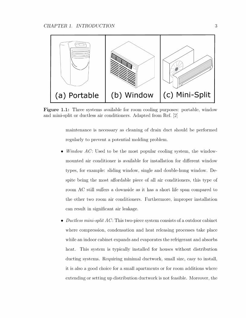
1.1 Three systems available for room cooling purposes: portable, window
and mini-split or ductless air conditioners. Adapted from Ref. [2] . . 3
1.2 Typical central air conditioning system with two main components:
the condenser unit and evaporator unit. Adapted from Ref. [3] . . . . 4
1.3 Percentage of different air conditioning systems installed within
Canada. Reproduced from data provided in Ref. [4] . . . . . . . . . . 6
1.4 Percentage of houses equipped with air conditioning systems across the
United States. Source: U.S. Energy Information Administration, 2009
Residential Energy Consumption Survey [2] . . . . . . . . . . . . . . 7
1.5 An example of VairTEX Air Director device applied on (a) residential;
(b) industrial condenser units . . . . . . . . . . . . . . . . . . . . . . 9
1.6 Two views of the VairTEX air director used in this study (a) isometric
view; (b) top view . . . . . . . . . . . . . . . . . . . . . . . . . . . . . 10
1.7 Typical VairTEX unit installation . . . . . . . . . . . . . . . . . . . . 11
2.1 Commonly used residential condenser fan blades (a) Rectangular-shape
two-blade; (b) Rectangular-shape three-blade; (c) Low-Noise three-
blade; (d) Rectangular-shape four-blade [23] . . . . . . . . . . . . . . 18
2.2 Schematic of Parker’s development on high efficiency air conditioner
condenser fan system . . . . . . . . . . . . . . . . . . . . . . . . . . . 19
xii

2.3 Model of outdoor air conditioner unit where (a) Old type outdoor unit;
(b) Optimized unit with double fan, extended bell mouth and sigma
shaped heat exchanger. Reproduced from Ref. [27] . . . . . . . . . . . 21
3.1 Schematic diagram of a basic ideal vapour-compression cycle in which
it consists of four components: compressor, condenser, throttle and
evaporator . . . . . . . . . . . . . . . . . . . . . . . . . . . . . . . . . 26
3.2 Typical T-s digram for actual and ideal vapour-compression refrigera-
tion cycle where subscript i, r and s stand for ideal cycle, actual cycle,
and isentropic stage respectively. Blue lines represent isobaric process
while red lines illustrate isothermal process . . . . . . . . . . . . . . . 28
3.3 Carrier air conditioning system and instrumentation - Adapted from
MAAE2400 Lab Manual . . . . . . . . . . . . . . . . . . . . . . . . . 29
3.4 Schematic of an evaporator unit where the dash line represents a con-
trol volume around the evaporator coil . . . . . . . . . . . . . . . . . 37
4.1 Dantec single-straight sensor 55P11. Adapted from dantecdynam-
ics.com [45] . . . . . . . . . . . . . . . . . . . . . . . . . . . . . . . . 41
4.2 Wheatstone bridge circuit in a constant temperature anemometer op-
eration mode where hot-wire probe acts as one of the resistors in the
bridge. Adapted from AA Lab Systems Ltd. [46] . . . . . . . . . . . . 42
4.3 Three Calibration Direction . . . . . . . . . . . . . . . . . . . . . . . 46
4.4 Three Directional Calibration Curves . . . . . . . . . . . . . . . . . . 47
4.5 Six positions of measurement for single hot-wire probe . . . . . . . . 48
4.6 Hot-wire probe coordinate u, v, and w at position 1 in related to flow
field coordinate system U, V and W . . . . . . . . . . . . . . . . . . . 55
4.7 General geometry of diffuser section where D1 is throat diameter, D2
is exit diameter, L is diffuser length and θ is conical angle. . . . . . . 57
xiii

4.8 Schematic of the convergent nozzle with matched fifth order polynomial
where R1 and R2 is are inlet and exit radii, L is the total length,
xm is the distance from the inlet to the match point where the two
polynomials of same curvature and slope meet [70] . . . . . . . . . . . 59
4.9 Schematic of a mini-version wind tunnel where calibrations in three
directions were performed . . . . . . . . . . . . . . . . . . . . . . . . 60
4.10 CTA mode calibration and correction curves from Hultmark’s study .
(a) Original calibration curves at different temperatures and (b) Curves
replotted using similarity variable given by Equation 4.44. Reproduced
from Ref [80] . . . . . . . . . . . . . . . . . . . . . . . . . . . . . . . 64
4.11 (a) In-house calibration curves at different temperatures and (b)
Curves replotted following Hultmark’s correction method . . . . . . . 64
4.12 Six-orientation measurement device where blue labels represent differ-
ent features of the main body part while orange labels show compo-
nents of the hollow tube part . . . . . . . . . . . . . . . . . . . . . . 66
4.13 Schematic of a 1D traverse system surrounding the condenser unit in
room ME2230-30 at Carleton University. Note that all dimensions are
in cm . . . . . . . . . . . . . . . . . . . . . . . . . . . . . . . . . . . . 68
4.14 Hot-wire measuring locations in reference to the condenser (a) and Air
Director (b) exit surfaces . . . . . . . . . . . . . . . . . . . . . . . . 69
4.15 Three velocity components: Radial (a), Axial (b) and Tangential (c)
were resolved after sampling at 1, 2, 4 and 8 kHz, where ‘’ represented
measurement taken for location 6 while ‘∗’ stood for data points of
location 7 . . . . . . . . . . . . . . . . . . . . . . . . . . . . . . . . . 71
xiv
4.16 Percent differences of average voltages between with and without TC
installed at six measuring positions referred to Figure 4.5 where P1,
P2, ...., and P6 represent position 1, position 2, ......., and position 6. 72
4.17 Percentage difference between temperature recorded at exact hot-wire
sensor and offset locations . . . . . . . . . . . . . . . . . . . . . . . . 73
5.1 Carrier air conditioning system and instrumentation - Adapted from
MAAE2400 Lab Manual . . . . . . . . . . . . . . . . . . . . . . . . . 77
5.2 Refrigerant temperatures recorded at five locations indicated in Figure
5.1 where (a), (b), (c), (d), and (e) corresponding to location 1, 2, 3,
4, and 5 with and without the AD added on the condenser exit surface
for two refrigerant flow meter readings 0.25 and 0.35 gal/min . . . . . 78
5.3 Air temperature recorded at the inlet and exit of evaporator for two
flow rates with and without AD applied on the condenser where (a)
and (b) correspond to inlet and outlet measurements, respectively . . 80
5.4 Pressured measured after (a) the condenser and after (b) the evapo-
rator with and without VairTEX AD installed for two interested flow
rates . . . . . . . . . . . . . . . . . . . . . . . . . . . . . . . . . . . . 81
5.5 Power consumed by the compressor were recorded with and without
VairTEX AD installed for two interested flow rates . . . . . . . . . . 82
5.6 A comparison of calculated refrigeration capacity with and without the
VairTEX AD on condenser unit at different flow rates . . . . . . . . . 84
5.7 Propeller frequency measured for two designated flow meter readings
with and without AD . . . . . . . . . . . . . . . . . . . . . . . . . . . 85
5.8 Amperage drawn by condenser fan with and without the VairTEX AD
installed . . . . . . . . . . . . . . . . . . . . . . . . . . . . . . . . . . 86
5.9 Computed COP for AC system . . . . . . . . . . . . . . . . . . . . . 87
xv

5.10 T-s diagram comparison with and without the AD at refrigerant flow
rate reading 0.35 gal/min . . . . . . . . . . . . . . . . . . . . . . . . . 88
5.11 Temperature captured at condenser surface discharge and VairTEX
AD exit top . . . . . . . . . . . . . . . . . . . . . . . . . . . . . . . . 89
5.12 Radial velocity component measured at condenser surface discharge
and VairTEX AD exit surface . . . . . . . . . . . . . . . . . . . . . . 91
5.13 Axial velocity contour collected at condenser surface discharge and
VairTEX AD exit surface . . . . . . . . . . . . . . . . . . . . . . . . . 93
5.14 Tangential velocity profile obtained at condenser surface discharge and
VairTEX AD exit surface . . . . . . . . . . . . . . . . . . . . . . . . . 94
xvi

Nomenclature
Latin Letters
A Cross section area [m2]
A,B,C Calibration constants [-]
A0, B0, C0 Values in generalized solution function [-]
A2/A1 Area ratio [-]
α Temperature coefficient of resistivity [C−1 ]
D Characteristic diameter [m]
d Hot-wire sensor diameter [m]
D1, D2 Diffuser throat and exit diameter [m]
δT Difference between wire and ambient temperatures [C ]
E Voltage [V ]
η Manipulative constant in covariance definition [-]
Ew Output voltage based on reference temperature [V ]
Ew,r Corrected output voltage based on reference temperature [V ]
xvii

F1, F2, F3 Generalized solution for six-orientation method [-]
G Pitch factor [-]
γZiZjCorrelation coefficient between two cooling velocities [-]
h Convection heat transfer coefficient [W/(m2K)
h Enthalpy [kJ/kg]
i, j Probe position [-]
K Yaw factor [-]
k Thermal conductivity of air [W/(mK)]
KZiZjCovariance of the effective cooling velocities [-]
L Diffuser/Nozzle length [m]
l Hot-wire sensor length [m]
Le Entrance length [m]
m Mass flow rate [kg/s]
n Exponent in power law equation [-]
Nu Nusselt number [-]
ω Propeller rotational speed [rev/s]
P Pressure [Pa]
P,Q,R Three selected measuring positions [-]
xviii

Pr Prandtl number [-]
Q Volume flow rate [m3/s]
Qin Refrigeration capacity [ton]
Qloss Heat loss from the system [W ]
Re Reynolds number [-]
ρ Fluid density [kg/m3]
Ro Reference resistance [Ω]
Rs Wire resistance [Ω]
s Entropy [kJ/kgK]
σ2 Variance [-]
t Integration period [-]
T Temperature [C]
Ta Ambient temperature [C]
θ Diffuser conical angle []
Tr Calibration (reference) temperature of hot-wire probe [C ]
Tw Wire temperature of hot-wire probe [C ]
U Radial velocity component [m/s]
µ Fluid dynamic viscosity [Ns/m2]
xix

u,v,w Orthogonal velocity components seen by the hot-wire [-]
υ Specific volume [m3/kg]
V Axial velocity component [m/s]
V Velocity [m/s]
ν Fluid kinemetic viscosity [m2/s]
V Volumetric flow rate [m3/s]
φ Inverse function of calibration equation [-]
W Tangential velocity component [m/s]
Winput Work input to the system [W ]
Z Effective cooling velocity [-]
Abbreviations
AC Air conditioning
AD Air director
AS Aspect ratio
CFC Chlorofluorocarbon
CFM Cubic feet per minute
COP Coefficient of performance
CR Contraction area ratio
xx

CTA Constant temperature anemometry
EER Energy efficiency ratio
GPM Gallon per minute
HFC Hydrofluorocarbon
HVAC Heating,ventilation, and air conditioning
HWA Hot-wire anemometer
LPM Litre per minute
NRCAN Natural Resources Canada
PIV Particle image velocimetry
RECS Residential energy consumption survey
RMS Root mean square
RPM Rotation per minute
SEER Seasonal energy efficiency ratio
SOM Six-orientation method
TC Thermocouple
xxi

Chapter 1
Introduction
Once considered a luxury, air conditioning has become an essential, bringing com-
fort for houses, shopping malls, hospitals, data centres, laboratories, as well as other
buildings that are vital to our daily lives and to our economy. Dr. John Gorrie -
a physician and inventor - initially proposed the idea of cooling a hospital for his
patients by using ice in the 1840s. Later, he began experimenting with the concept
of artificial cooling by designing an ice machine powered by a compressor and was
granted a patent in 1851. Even though Gorrie was unable to market his technology,
his idea and invention clearly laid a foundation for modern air conditioning and refrig-
eration systems [1]. Engineer Willis Carrier continued the quest for creating artificial
cooling while working at Buffalo Forge Company in 1902. The first modern electrical
air conditioning (AC) unit was created and patented, as Carrier solved a humid-
ity problem on magazine papers at Sackett-Wilhelms Lithographing and Publishing
Company in Brooklyn.
In later years, Carrier debuted cooling systems, which were modified from his pre-
vious design for the Metropolitan Theatre in Los Angeles and the Rivoli Theatre in
New York. Despite advancements in cooling technologies, there were still challenges
implementing these cooling systems for residential use due to their size and cost.
1

CHAPTER 1. INTRODUCTION 2
Frigidaire introduced a split-type room cooler system to the market in 1929 while
Frank Faust improved this design by customizing a self-contained room cooler. In
1932, Schultz and Sherman patented a window-ledge air conditioning unit. A more
compact and less expensive version of a window air conditioner became popular in
1947 by development of Henry Galson. Finally, in the 1970s, central air conditioning
systems made their way into American homes. However, after this period, modifi-
cations on air conditioning systems mainly focused on operating the system more
environmentally friendly or increasing the efficiency.
This chapter classifies residential air conditioning systems currently in-use in
Canada and the United States and provides statistical information on the penetra-
tion of different types of air conditioning systems across both countries. Finally, the
motivation that drives this work as well as the structure of the thesis will also be
presented.
1.1 Classification of Air Conditioning System
For residential use, depending on budget, existing set-up, and area required for cool-
ing, there are two basic systems to choose from:
1. Room air conditioners: These air conditioners offer low-cost approach, min-
imum installation effort yet effective to provide comfort in small spaces such
as a single room apartment, individually room temperature setting , etc. This
type can be categorized into three divisions: portable, window, and ductless
mini-split, as shown in Figure 1.1 (a),(b) and (c).
• Portable AC : This free-stand evaporative cooler unit is easily moved be-
tween rooms and requires temporary ducting to the outdoors. However,

CHAPTER 1. INTRODUCTION 5
Most central AC systems run on the vapour-compression principle. The refriger-
ant is compressed and condensed at the condenser unit. Then heat from refrig-
erant is released outside so that the cooled/liquid refrigerant can be expanded
and sent to the evaporator unit. As a thermostat detects a rise of temperature,
the air handling unit draws hot air from various parts of the house and pushes
it across the evaporator coil where heat exchanging between hot air and cool
refrigerant takes place. As a result, air is cooled down and forced back into the
house through other ducts. The cycle is repeated until the desired temperature
reaches throughout the house. Schematic of a central AC system can be seen
in Figure 1.2. A central AC system is proven to be a cost-effective option if
ductwork exists in the house. Also, it is more quiet, efficient and convenient to
operate and produces better air quality control for an entire house than window
types.
1.2 Statistical Facts on an Air Conditioning Sys-
tem
According to the most recent energy survey conducted by Natural Resources Canada
(NRCAN) in 2011, almost 60% of Canadian households had an air conditioning sys-
tem although there were distinct variations amongst the Atlantic, Alberta and the
remainder parts of Canada, as depicted in Figure 1.3.
Across Canada, for those who had an air conditioner installed, over 30% had
central air. Again, the penetration rate was different amongst regions, notably - the
most populated province (Ontario) almost 80% of more than 4 million households
had a central air system, compared to the Atlantic region where approximately only

CHAPTER 1. INTRODUCTION 6
0%
20%
40%
60%
80%
100%
Canada ATL QC ON MB/SK AB BC
Central AC Window AC No AC
Figure 1.3: Percentage of different air conditioning systems installed within Canada.Reproduced from data provided in Ref. [4]
20% of households owned the same system [4]. Moreover, the amount of cooling floor
space almost tripled in 2011 compared to in 1990. It means that more Canadians
live in larger and air-conditioned homes. Therefore, this resulted in the rising energy
consumption of 150% (from 10 PJ to 25 PJ) over the same period [5]. The increase in
energy consumption would have been more profound if there was no energy efficiency
regulations established. According to the NRCAN, on average - an ENERGY STAR
certified system uses 8% less energy than a standard model [6]. This certification
requires a central air conditioners’ seasonal energy efficiency ratio (SEER) rating of
minimum 13.0, where SEER is the cooling output during annual cooling season [Btu],
divided by the total electricity consumed by the air conditioning system during the
same season [7]. However, only 36% of central air systems possessed an ENERGY
STAR label across Canada. Definitely, there was no other option than to replace old

CHAPTER 1. INTRODUCTION 7
systems with more modern units, for those 64% remaining that were still running
inefficiently.
1981 1984 1987 1990 1993 1997 2001 2005 2009
0%
20%
40%
60%
80%
100%
South Midwest Northeast West
Figure 1.4: Percentage of houses equipped with air conditioning systems across theUnited States. Source: U.S. Energy Information Administration, 2009 ResidentialEnergy Consumption Survey [2]
In the United States, a steady rise in air conditioner possession in all regions has
been observed among all types of housing from 1981 and since 2009 this piece of
equipment has become standard in most U.S. homes. As demonstrated in Figure 1.4,
the latest survey revealed that on average 87% of households were equipped with AC
systems, while the southern states have approached 100% AC coverage.
Of those homes equipped with AC system, Table 1.1 below demonstrates regional
difference between various types of AC system. In particular, central air systems were
most commonly used in the Midwest, South and West regions while in the Northeast
region, it was more common to see room air conditioners. In addition, housing type
and age also drove variation in type of AC systems. As result, some houses had
both central and window air conditioners as the total added up to more than 100%.
CHAPTER 1. INTRODUCTION 8
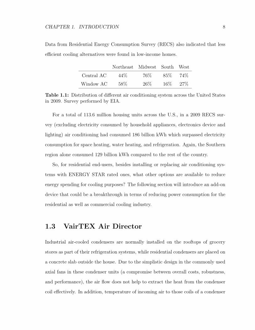
Data from Residential Energy Consumption Survey (RECS) also indicated that less
efficient cooling alternatives were found in low-income homes.
Northeast Midwest South West
Central AC 44% 76% 85% 74%
Window AC 58% 26% 16% 27%
Table 1.1: Distribution of different air conditioning system across the United Statesin 2009. Survey performed by EIA.
For a total of 113.6 million housing units across the U.S., in a 2009 RECS sur-
vey (excluding electricity consumed by household appliances, electronics device and
lighting) air conditioning had consumed 186 billion kWh which surpassed electricity
consumption for space heating, water heating, and refrigeration. Again, the Southern
region alone consumed 129 billion kWh compared to the rest of the country.
So, for residential end-users, besides installing or replacing air conditioning sys-
tems with ENERGY STAR rated ones, what other options are available to reduce
energy spending for cooling purposes? The following section will introduce an add-on
device that could be a breakthrough in terms of reducing power consumption for the
residential as well as commercial cooling industry.
1.3 VairTEX Air Director
Industrial air-cooled condensers are normally installed on the rooftops of grocery
stores as part of their refrigeration systems, while residential condensers are placed on
a concrete slab outside the house. Due to the simplistic design in the commonly used
axial fans in these condenser units (a compromise between overall costs, robustness,
and performance), the air flow does not help to extract the heat from the condenser
coil effectively. In addition, temperature of incoming air to those coils of a condenser

CHAPTER 1. INTRODUCTION 9
could be influenced by the heated flow escaping from the condenser outlet due to
its exit angles [8]. A study from Khankari also indicated that with an increase in
crosswind, the hot plume discharging from the condenser exit bent downward and
almost reached the ground in case of higher wind speed [9].
Invented by Gerard Godbout - founder of VairTEX Canada Inc. to address the
inefficiencies of commercial, industrial and residential cooling and refrigeration sys-
tems, the Air Director (AD) is a passive energy reduction device which can be added
to the top of the axial fans of industrial or residential condensers.
(a) (b)
Figure 1.5: An example of VairTEX Air Director device applied on (a) residential;(b) industrial condenser units
As illustrated in Figure 1.5, VairTEX units were neatly placed on top of residential
and industrial condensers. The passive device has cylindrical structure with six fixed
blades that redirect the flow upwards with additional swirling and mass flow. Hence,
this device helps improve the performance of the AC unit by reducing power con-
sumption of electrical fan motors. According to VairTEX US Patent document [10],
the Air Director consists of three main components:

CHAPTER 1. INTRODUCTION 10
1. Cylindrical body: is used to direct the air flow exiting the condenser. The
tube’s diameter has the same dimension as the condenser exit.
2. Fixed blades: a series of six fixed blades is attached to the interior of a tube in
order to generate turbulence
3. Top cowling: is designed to reduce diameter of the cylindrical tube, hence
accelerates the exit flow. This section is attached to the upper part of a tube.
Depending on existing configuration of condenser fan (i.e. clockwise or counter-
clockwise rotation), the VairTEX AD blades are configured in counter arrangement.
For example, if the condenser fan rotates in a clockwise direction, VairTEX AD blades
will be positioned in counter-clockwise direction. Due to variation in condenser sizes,
the tube diameter is customized to produce a seamless add-on device.
30.5
cm
22 c
m
Fixed blade
Top cowling
Cylindrical
body
(a)
48.26 cm
57.15 cm
1
2
3
4
5
6
(b)
Figure 1.6: Two views of the VairTEX air director used in this study (a) isometricview; (b) top view
Figure 1.6 illustrates isometric and top views of the residential Air Director units
along with its dimensions that will be used in this study. The cowling creates a total
CHAPTER 1. INTRODUCTION 11
reduction of 3.5′′ (8.9 cm) from the main body. Six blades with width of 4′′ (10.2 cm)
each are fixed at 75 from horizontal plane. It should be noted that as blades are
only jointed in pairs (i.e. 1 and 6, 2 and 5, 3 and 4), this leaves 2 small gaps in the
centre of the device.
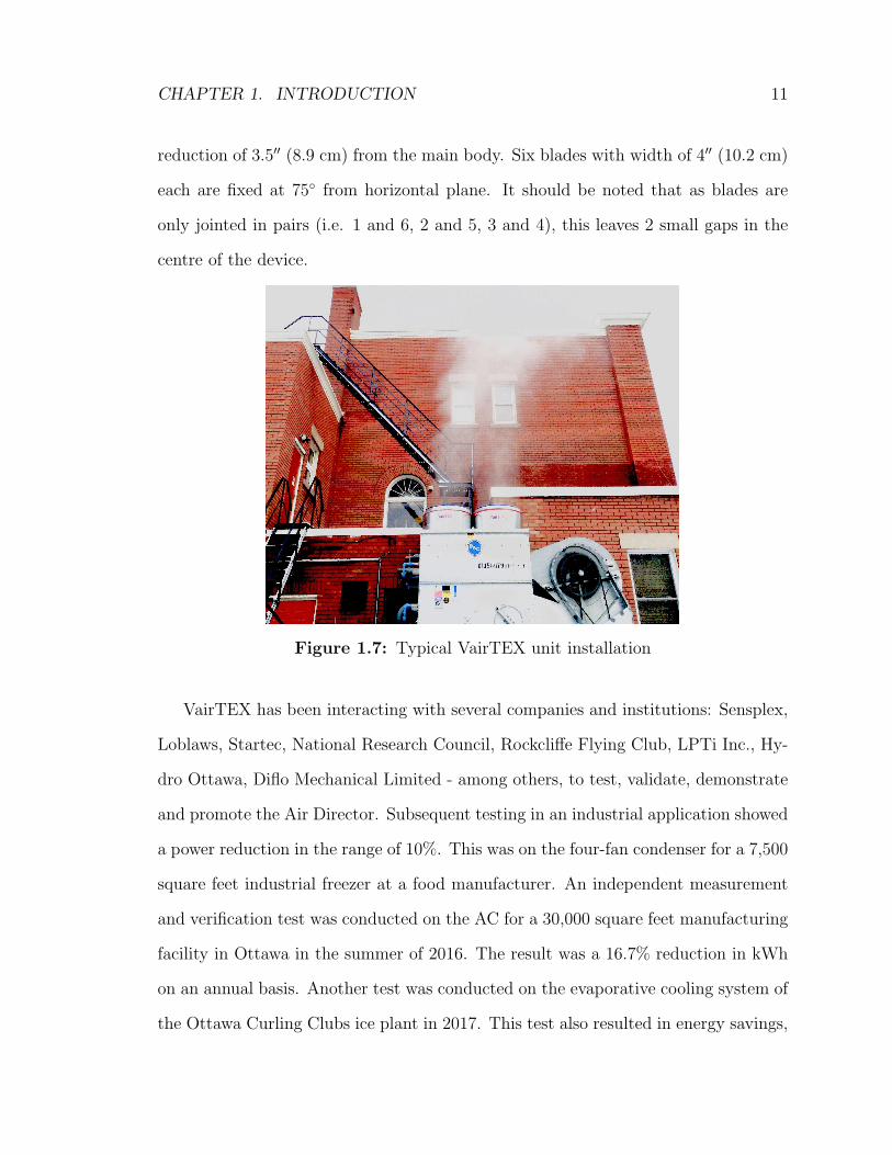
Figure 1.7: Typical VairTEX unit installation
VairTEX has been interacting with several companies and institutions: Sensplex,
Loblaws, Startec, National Research Council, Rockcliffe Flying Club, LPTi Inc., Hy-
dro Ottawa, Diflo Mechanical Limited - among others, to test, validate, demonstrate
and promote the Air Director. Subsequent testing in an industrial application showed
a power reduction in the range of 10%. This was on the four-fan condenser for a 7,500
square feet industrial freezer at a food manufacturer. An independent measurement
and verification test was conducted on the AC for a 30,000 square feet manufacturing
facility in Ottawa in the summer of 2016. The result was a 16.7% reduction in kWh
on an annual basis. Another test was conducted on the evaporative cooling system of
the Ottawa Curling Clubs ice plant in 2017. This test also resulted in energy savings,

CHAPTER 1. INTRODUCTION 12
and more importantly the exhaust water vapour was directed up and away from the
building, as shown in Figure 1.7. Moreover, VairTEX’s business partner in the United
State reported an energy reduction in the range of 16-21% [11].
The VairTEX Air Director is a clean-technology - as it reduces energy consump-
tion of the AC systems, requires no moving parts or maintenance, ease of installation,
with seamless integration with the design of existing condensers. Several years of ex-
tensive testing on commercial condensers of various sizes and brands have consistently
demonstrated the following benefits:
1. Increased air flow hence reduced energy consumption by the condenser
2. Lower head pressure therefore increased thermal exchange
3. Lower ambient intake air temperature by restricted air recirculation at the con-
denser
4. Protection of the interior components of the condenser from the elements
5. Meeting or exceeding the rated refrigeration capacity with less energy consump-
tion
6. Superior condenser performance in adverse weather conditions (i.e cross wind)

CHAPTER 1. INTRODUCTION 13
1.4 Motivation
Through their collaboration with several industrial partners, the VairTEX Air Di-
rector has proven its effectiveness in air conditioning and refrigeration systems by
reducing power consumption. Besides the commercial/industrial market, VairTEX
Canada Inc. is also interested (long term) in pursuing residential market in Canada
and in the United States. For residential air conditioning systems, there has not
been any verification regarding VairTEX device’s benefits as well as quantifying the
differences when applying the device. To successfully promote VairTEX’s product to
residential customers, it is crucial to perform a study in order to provide quantitative
and qualitative results scientifically. Moreover, statistical surveys on household elec-
tricity consumed by air conditioners in Canada and in the United States indicated
that hundreds of billions kWh have been used for cooling purpose. In terms of envi-
ronmental concerns, 1% decrease in the amount of electricity would benefit not only
the users but also the environment.
The work performed in this thesis was a collaboration between the Department of
Mechanical and Aerospace Engineering and VairTEX Canada Inc. to conduct exper-
imental testing of the VairTEX Air Director on residential air conditioning system.
Thermodynamic analysis was performed to show the advantages of the Air Director
listed above. In addition, the hot-wire six-orientation measurement technique was ex-
plored and implemented to yield mean velocities in three directions at the condenser
exit. Velocity measurements were used to confirm the air flow increase created by the
Air Director.

CHAPTER 1. INTRODUCTION 14
1.5 Structure of Thesis
This thesis consists of 6 chapters. Chapter 2 provides a literature review on existing
add-on devices for cooling/refrigeration systems and also on similar performance-
enhancing add-on devices in wind turbines. Chapter 3 introduces the principle of
vapour-compression cycle in residential air conditioning system and compares the
ideal and actual cycles. The air conditioner experimental set-up and the data re-
duction procedures are also outlined in Chapter 3. Chapter 4 starts up with the
fundamental concept of hot-wire measuring technique, followed by detailing the the-
ory and implementation of the six-orientation hot-wire measurement technique, as
well as the temperature correction technique. This chapter also describes the calibra-
tion set-up along with the experimental set-up for hot-wire measurements. Next, in
Chapter 5, results and discussions of experimental data are presented, in addition to
the uncertainty analysis. Finally, Chapter 6 draws a conclusions on the project and
provides some suggestions for future work.

Chapter 2
Literature Review and Background
Air conditioning systems are used to provide living comfort condition for humans in
residences. Air conditioning is defined as “the process of treating air in an internal
environment to establish and maintain required standards of temperature, humidity,
cleanliness, and motion” [12]. Air-cooled condensers in a residential central AC system
are widely used due to its cost-effective and satisfactory performance as opposed to a
more expensive option, requiring intensive maintenance (water cooling). However, the
performance of these condensers is greatly affected by the ambient air temperature
surrounding the condenser.
Residential air-cooled condensers are often constructed with copper finned tube to
allow heat exchange between the refrigerant and the surrounding environment. Heat
is transferred to the attached fins as hot refrigerant passes through the condenser
coil. An electrically powered axial fan draws air from outside, across those fins to
remove heat from the refrigerant and allows condensation and sub-cooling processes
of refrigerant taking place prior to the expansion valve. The majority of residential
central AC systems apply the principle of a vapour-compression refrigeration cycle.
The cycle coefficient of performance (COP) depends upon various parameters, for
example: pressures at sub-cooling and superheating processes, compressor’s inlet and
15

CHAPTER 2. LITERATURE REVIEW AND BACKGROUND 16
outlet pressures. In addition, the COP is largely impacted by power demanded from
the compressor as this is the major power consumption in the system. As condenser
temperature rises, its pressure increases and as a consequence, the compressor requires
more work. Moreover, high condenser temperature also reduces cooling capacity of
the cycle due to the reduction of liquid content in the evaporator [13]. Hence, high
condenser temperatures are not desirable as COP of the system decreases.
2.1 Improving Air Conditioning Performance
Several efforts to increase COP focused on improving compressor performance. For
example, Kandpal (1978) examined high performance of an air conditioner compressor
by the use of low loss steel (better grade of steels) in the motors, capacitor start and
run (CSR) design motors, or higher values of run capacitance, improved muffling, or
gas handling and valves [14]. Sakuda et al. (2001) introduced a scroll compressor
type with new sealing-oil supply mechanism to optimized oil flow rate in order to
achieve performance improvement of the compressor [15].
Recently, research attempted to improve AC system performance by investigat-
ing shading effect on the condenser. Sonne et al. (2002) conducted experimental
study on three homes over a two year period to quantify space cooling energy savings
from shading condenser units. However, the most optimistic result demonstrated an
improvement of air conditioner efficiency by only 1% [16]. Furthermore, this study
also indicated the potential hazards of localized condenser shading as some shading
methods (for example: planting trees and shrubs) may interfere with airflow across
the condenser. A study from ElSherbini and Maheshwari (2010) concluded that AC
performance efficiency would not exceed a maximum of 1% suggested that shading
method alone, without evapo-transpiration, is not effective to boost AC performance
CHAPTER 2. LITERATURE REVIEW AND BACKGROUND 17
nor reduce electrical demand [17]. Donovan and Butry (2009) estimated a saving of
5.2% in electricity consumption in summertime when trees were planted on the west
and south sides of 460 single-houses in Sacramento, California [18].
Another alternative way to improve residential air conditioning system is to intro-
duce an evaporative condenser. Hoeschele et al. (1998) pointed out that evaporative
condensers may become the next generation for residential AC systems as this tech-
nology can provide significant operating cost savings in hot and dry climates [19].
Furthermore, Parker et al. (2014) reported an improvement in AC efficiency by 20-
30% by combining high efficiency fan and diffuser stage coupling with an evaporative
condenser pre-cooler [20].
Improving air flow across the condenser could help lower power consumption, thus
increase the COP of the system. Elsayed and Hariri suggested in their study that
a 10% reduction in compressor power consumption was achieved by increasing the
condenser air flow of about 50% in split-type air conditioners [21]. So the problem
can be solved by optimizing the axial-flow fan, a design not changed in decades.
There are three types of axial-flow fans: propeller, tube-axial and vane-axial. Out
of these three, the propeller type fans are widely used in both residential and commer-
cial air conditioning systems. They deliver large volume of air with less horsepower
than the centrifugal fans but can develop low static pressure problem. As the sys-
tem resistance increases, the horse-power also increases. This is in contrast to the
centrifugal fan in which the horsepower decreases with an increase in the system re-
sistance. Thus a propeller fan used for an air-cooled condenser can draw more electric
current when the condenser fins get choked with dust. Also, the air quantity delivery
goes down [22]. Overall fan performance is sacrificed by robustness, cost and ease
of manufacturing. Clearly, the blade design is one of the problems. Condenser axial
fans are commonly made by extruding or stapling aluminium sheets. The number

CHAPTER 2. LITERATURE REVIEW AND BACKGROUND 18
of blades varies from two to four, while two common shapes can be found in HVAC
company catalogues, as illustrated in Figure 2.1.
(a) (b)
(c) (d)
Figure 2.1: Commonly used residential condenser fan blades (a) Rectangular-shape two-blade; (b) Rectangular-shape three-blade; (c) Low-Noise three-blade; (d)Rectangular-shape four-blade [23]
At the Seventh Turbomachinery Symposium in Houston Texas in 1978, Robert C.
Monroe presented his paper on ‘Improving Cooling Tower Fan System Efficiencies’ in
which he identified the inefficient air flow from poorly design conventional fan blades.
Monroe concluded that increasing air flow would significantly improve the efficiency
of the condenser. However, he also claimed that to increase the air flow by 10% would
require an additional 35% in energy consumption [24].

CHAPTER 2. LITERATURE REVIEW AND BACKGROUND 19
In order to increase air flow across the condenser unit, the condenser fan blade
could follow a similar process as in aerospace industry by re-designing and optimizing
its shape. However, within the extent of the current literature survey, no full optimiza-
tion effort for the condenser fan blade design was found in the literature. A different
approach was presented by Danny S. Parker et al. (2005) in which true-airfoil flat
fan blades were embedded in a conical diffuser [25]. Unlike a conventional condenser,
where whole fan assembly (blades and motor) was surrounded by condenser coils, the
new design fan assembly was covered by a conical diffuser housing situated on top of
those coils. Figure 2.2 shows the design schematic of the enhanced fan system.
ACOUSTIC
FIBROUS
INSULATION
DOME SHAPED GRILL
CONICAL CENTER BODY
CONICAL DIFFUSER
A
VIEW 'A'
SCALE: 500''=1''
CONICAL DIFFUSERVORTEX SHEDDING
CONTROL STRIP
TIP
CLEARANCE
SCALE:125''=''1
Figure 2.2: Schematic of Parker’s development on high efficiency air conditionercondenser fan system
In Parker’s study, his objective was to create the most efficient design with robust
characteristics and provide good performance over a range of static pressure while
reducing fan noise at the same time. A total of five designs were developed based
on blade shapes and blade numbers (ranging from 3 to 5 blades) where each design

CHAPTER 2. LITERATURE REVIEW AND BACKGROUND 20
was consisted with different sub-variations. The most striking design - coded as fan
A5 was composed of 5 asymmetrical blades (centred unevenly around the rotating
motor hub) which followed the technology explored to reduce noise level for helicopter
rotors in 1999 by Kernstock [26]. As sound rushed through uneven spacings between
blades, resonance frequency was reduced and hence a lower ambient sound level was
produced from the condenser unit. Over one hundred tests for all fan designs were
conducted at 850 RPM and 1075 RPM.
Based on the relationship between high efficiency propeller design and its housing,
Parker’s diffuser was extended to a length of 18′′ (46 cm) to provide an additional 25%
pressure recovery while divergent angle had a value of 7. The diffuser increased its
diameter from 19.75′′ (50 cm) to 24′′ (61 cm) at the grill top providing both aesthetic
appearance and sizing acceptance from consumers. The motor and fan blades were
located at the bottom of the assembly. Through trial and error, the design was refined
to a smooth conical centre body to increase air flow across the fan blade and thus
reduce power consumption.
Parker’s research can be summarized into two main parts. First, for the con-
ventional condenser’s motor and body, a new twisted and tapered propeller air foils
demonstrated greater air moving efficiency, which defined as the ratio between air
flow rate [ft3/min] over power consumption [W], while saving 21% of power consump-
tion. Secondly, the study also revealed that by inserting an elongated conical diffuser
after the fan motor, air moving efficiency [ft3/minW] was improved by over 16% for
standard Original Equipment Manufacturer (OEM) fans and over 27% for high per-
formance fans designed in Parker’s project. Through the use of porous foam strip,
air flow performance increased while helping to reduce noise level. Moreover, when
equipped with an enhanced diffuser, fan A5 allowed an increase in air moving effi-
ciency of 46% or equivalent to a 5% addition in air flow [ft3/min], and also reduced

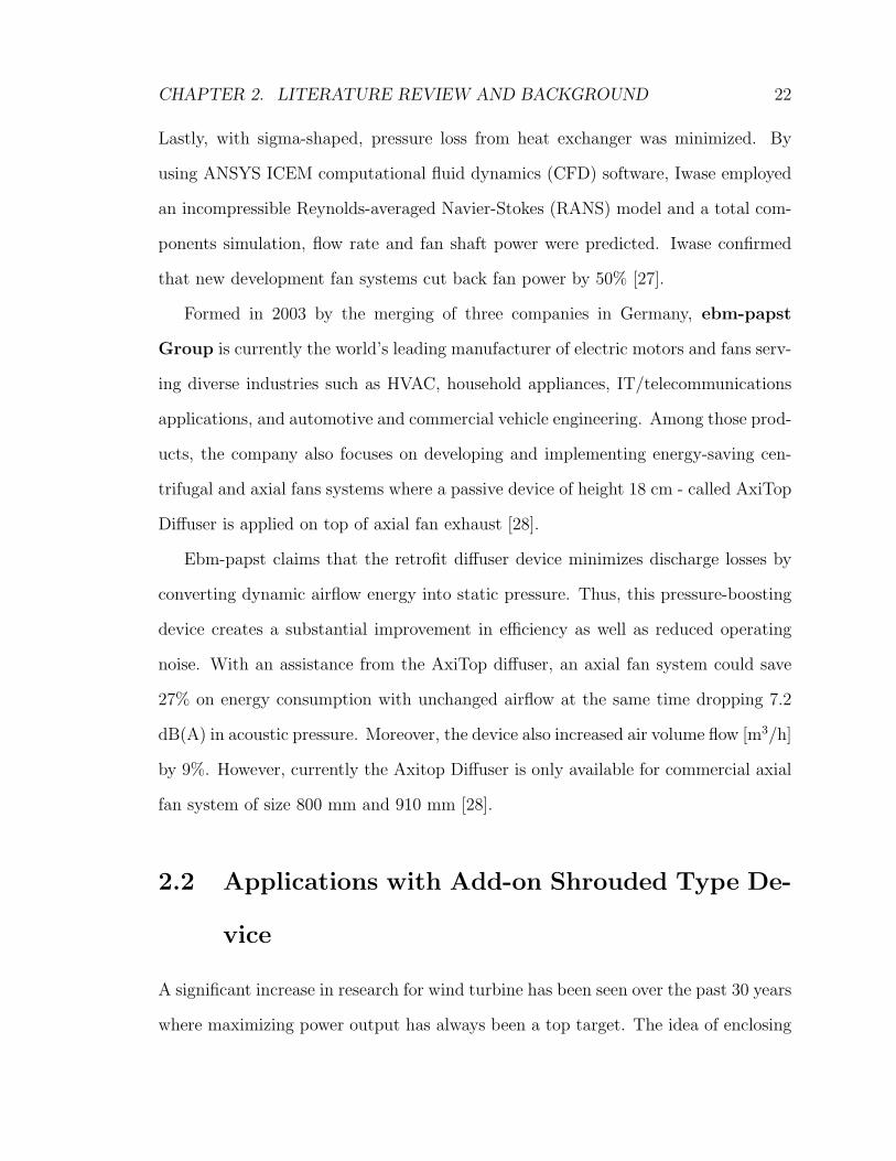
CHAPTER 2. LITERATURE REVIEW AND BACKGROUND 22
Lastly, with sigma-shaped, pressure loss from heat exchanger was minimized. By
using ANSYS ICEM computational fluid dynamics (CFD) software, Iwase employed
an incompressible Reynolds-averaged Navier-Stokes (RANS) model and a total com-
ponents simulation, flow rate and fan shaft power were predicted. Iwase confirmed
that new development fan systems cut back fan power by 50% [27].
Formed in 2003 by the merging of three companies in Germany, ebm-papst
Group is currently the world’s leading manufacturer of electric motors and fans serv-
ing diverse industries such as HVAC, household appliances, IT/telecommunications
applications, and automotive and commercial vehicle engineering. Among those prod-
ucts, the company also focuses on developing and implementing energy-saving cen-
trifugal and axial fans systems where a passive device of height 18 cm - called AxiTop
Diffuser is applied on top of axial fan exhaust [28].
Ebm-papst claims that the retrofit diffuser device minimizes discharge losses by
converting dynamic airflow energy into static pressure. Thus, this pressure-boosting
device creates a substantial improvement in efficiency as well as reduced operating
noise. With an assistance from the AxiTop diffuser, an axial fan system could save
27% on energy consumption with unchanged airflow at the same time dropping 7.2
dB(A) in acoustic pressure. Moreover, the device also increased air volume flow [m3/h]
by 9%. However, currently the Axitop Diffuser is only available for commercial axial
fan system of size 800 mm and 910 mm [28].
2.2 Applications with Add-on Shrouded Type De-
vice
A significant increase in research for wind turbine has been seen over the past 30 years
where maximizing power output has always been a top target. The idea of enclosing

CHAPTER 2. LITERATURE REVIEW AND BACKGROUND 23
the wind turbine inside a specially designed shroud has been suggested in numerous
papers and research [29]. A shrouded wind turbine, also called wind lens, is a new
type of wind power system where a simple ring structure encloses the rotor, causing
greater wind to pass through the turbine. As a consequence, the turbine’s efficiency
of capturing energy from the wind gets dramatically increased. Wind lens appear in
different shape which resulted in several configurations, for example: straight diffuser,
nozzle-diffuser combination, brimmed diffuser augmented and nozzle augmented wind
turbine. By increasing the mass flow, a wind turbine with a brimmed diffuser has
demonstrated 2 - 5 times additional power extraction from a bare wind turbine, given
the same rotor diameter and incoming wind speed [30, 31].
Kosasih et al. (2012) reported an experimental comparison on different diffuser
augmented horizontal axis micro wind turbine type. His study revealed that straight
diffuser enhanced performance by 56% compared to a bare wind turbine while the
nozzle-diffuser improved performance by 61% - slightly better than diffuser only [32].
For nozzle augmented type wind turbine, Balaji et al. (2014) confirmed a greater
power output (of approximately 40%) by nozzle augmented wind turbine as opposed
to a bare horizontal axis wind turbine [33]. In addition, study from Pambudi et.al
(2017) confirmed nozzle lenses successfully increase the efficiency of wind turbines
where wind was insufficient to drive turbine blades [34].
Through several examples found in literature and despite variation in shapes and
configurations of shrouded structure around the wind turbines, their performance
were proven to be greatly improved as opposed to a bare conventional wind turbine.
Passive (add-on) devices have proven to improve performance of not only AC
systems but also for wind turbines. Therefore, the effectiveness of the AD is promis-
ing and will be evaluated on residential AC system, located in the Thermodynamic
Laboratory at Carleton University. Two main performance parameters: refrigeration

CHAPTER 2. LITERATURE REVIEW AND BACKGROUND 24
capacity and coefficient of performance will be investigated.
Chapter 3
Air Conditioning Performance with The
Add-on VairTEX Air Director
3.1 Principle of Vapour-Compression Air Condi-
tioning Systems
Vapour-compression cycle is no doubt the most commonly used method which has
been widely applied for both residential and commercial cooling purposes, for exam-
ple: refrigerators, freezers, air conditioners, hockey rinks, etc. In 1920s, a large num-
ber of refrigerants used in the vapour-compression cycle was compounds of ammonia
and sulphur dioxide. These compounds however, were toxic and flammable. Subse-
quently, they were replaced by halogenated paraffin hydrocarbons refrigerants, also
called chlorofluorocarbons (CFCs). These CFCs were marketed under trade names
such as Freon R© (R-12) and Genetron R© (R-22) [35]. CFC-based refrigerants were
discovered to cause ozone depletion in the stratosphere by professor F. Rowland and
his post-doctoral fellow M. Molina [36]. Due to this reason, CFC refrigerants were
substituted by hydrofluorocarbons (HCFs), which include R-134a, R-407C or R-410A.
Schematic diagram of a basic vapour-compression cycle is illustrated in Figure 3.1,
25

CHAPTER 3. AC PERFORMANCE WITH ADD-ON VAIRTEX AD 26
followed by the details of its operation which can be described in 4 processes.
Compressor
Condenser
Throttle
Evaporator
1
2
3
4
Saturated
Vapour
Superheated
Vapour
Saturated
Liquid
Liquid-Vapour
Mixture
Qout
Qin
Win
Figure 3.1: Schematic diagram of a basic ideal vapour-compression cycle in whichit consists of four components: compressor, condenser, throttle and evaporator
1. Compression (state 1 - state 2): The refrigerant in saturated vapour form enters
the compressor at low pressure, low temperature. Here, the compression process
takes place to raise the pressure and temperature of the refrigerant. At this
point, the refrigerant is hotter than the surrounding environment and leaves
the compressor to enter the condenser as superheated vapour.
2. Condensation (state 2 - state 3): The condenser fan draws air from the sur-
rounding environment to flow across the condenser coil. The heat is transferred
from the refrigerant to air at constant pressure. Hence, the temperature of the

CHAPTER 3. AC PERFORMANCE WITH ADD-ON VAIRTEX AD 27
refrigerant is reduced to its saturation point and changed to its saturated liquid
phase.
3. Throttling and expansion (state 3 - state 4): The refrigerant then enters the
throttling valve which expands and releases its pressure. As a result, the refrig-
erant becomes a liquid-vapour mixture at low temperature.
4. Evaporation (state 4 - state 1): The cooling effect takes place at the evaporator
as refrigerant passes through the evaporator coil and causes a heat exchange
between room warm air, drawn in by an evaporator fan, and cold refrigerant.
The air is cooled and is distributed back to the room while the refrigerant un-
dergoes a phase change to become saturated vapour and enters the compressor
to repeat the cycle.
The performance of the vapour-compression refrigeration cycle can be further
investigated on a T-s diagram, as shown in Figure 3.2 where yellow and green loops
represent ideal and actual cycle, respectively. It can be seen that several features of the
actual cycle depart from the ideal cycle. The heat transfer between the refrigerant
and the warm and cold regions are not accomplished reversibly. Specifically, the
refrigerant temperature in the condenser is greater than the warm region temperature
TH in the ideal cycle, while on the other hand, the refrigeration temperature in the
evaporator is less than the cold region temperature TC in the ideal cycle. As a
result, the coefficient of performance (COP) decreases as the average temperature
of the refrigerant in the evaporator decreases and as the average temperature of the
refrigerant in the condenser increases [37].
For the actual cycle, the dashed line in Figure 3.2 suggests an isentropic process
where specific entropic remains constant during the entire compression stage. How-
ever the actual cycle experiences an adiabatic irreversible process which increases the


CHAPTER
3.
AC
PERFORMANCEW
ITH
ADD-O
NVAIRTEX
AD
29
6
5
4
1
2
3
7
Air Flow
Condenser Fan
Compressor
Condenser
Flow meter
Sight Glass
Sight Glass
Sight Glass
Throttle
Evaporator
Evaporator FanPropeller
Anemometer
Air FlowAmbient Air
Evaporator
Pressure Gauge
Condenser
Pressure Gauge
1.24 m
Condenser
Evaporator
Axis of
Rotation
Wall Ceiling
Ground
2.1 m
3.7 m
Side View Front View
Figure 3.3: Carrier air conditioning system and instrumentation - Adapted from MAAE2400 Lab Manual
CHAPTER 3. AC PERFORMANCE WITH ADD-ON VAIRTEX AD 30
3.2 Experimental Set-up
A typical residential Carrier air conditioner, which is installed in room ME 2230
(Thermodynamics Laboratory), is equipped with temperature, pressure and power
measurement instruments. The vapour-compression refrigeration cycle in this system
uses R-22 as the refrigerant. The air conditioner consists of two main units: evap-
orator and condenser units. The evaporator coil and evaporator fan make up the
evaporator unit while the condenser unit comprises of a compressor, condenser coil
and the condenser fan. Being attached to the wall, the evaporator unit is installed
above the condenser unit. The condenser, on the other hand, is mounted on the floor
where its fan centre of rotation is 1.24 m away from that wall. Also there is an open
perimeter around both evaporator and condenser units. Schematic of the set-up is
illustrated in Figure 3.3. The data collected from these instruments are used in the
performance analysis for two study cases: with and without the VairTEX Air Direc-
tor. The description for each instrument and component in this set-up are described
in the following section.
3.2.1 Evaporator unit
The evaporator fan forces air to pass through rifled copper tubes which contains
the refrigerant. It has three operational speeds which can be controlled through a
switch located at the control panel. The corresponding power consumption by the
fan is listed in Table 3.1. Despite three speed settings available, preliminary study
indicated that evaporator fan speed did not change COP value of the system between
two study cases: with and without the AD. Hence, experiments performed on the AC
system with and without AD used the ‘low’ setting for evaporator fan speed.

CHAPTER 3. AC PERFORMANCE WITH ADD-ON VAIRTEX AD 31
Fan Setting Power Consumption [kW]
Low 0.26
Medium 0.30
High 0.36
Table 3.1: Power consumption for different evaporator fan speeds [38]
3.2.2 Condenser unit
The condenser copper coil is surrounded by aluminium fins in order to increase surface
area, hence to enhance heat transfer between air and refrigerant. Air flow through
the condenser unit is driven by a General Electric motor. The specifications of the
motor are shown in the table below.
Air Flow [CFM] 1900
Horse Power [HP] 1/12
Voltage [V] 208-230
Amperage [A] 0.50
Rotation [RPM] 1100
Phase 1
Frequency [Hz] 60
Table 3.2: Condenser fan specification
The compressor is a hermetic-scroll type which operates at 3450 rev/min. It is
equipped with an internal temperature-sensitive and current-sensitive overload sensor.
A Wavetek DM7 power meter is calibrated in V-DC scale to measure power consumed
by the compressor in kW. The accuracy of the power meter is 0.8% on DC Voltage
setting [39].

CHAPTER 3. AC PERFORMANCE WITH ADD-ON VAIRTEX AD 32
3.2.3 Throttle
The throttle is a stainless steel metering valve with an 8 stem point and 0.125′′
orifice. To prevent complete shut off, a spacer is installed in the valve.
3.2.4 Refrigerant flow meter
A V-groove flow meter type, from Kobold Intruments Inc., was used to adjust refrig-
erant flow rate. The meter’s range is from 0.1 - 0.7 gal/min (0.38 - 2.65 L/min) with
an accuracy of approximately ± 4% of the full scale.
3.2.5 Pressure gauges
Two Ashcroft 2071A Contractor pressure gauges (range from vacuum - 600 psi) were
used to measure pressures of the refrigerant after the condenser and after the evapora-
tor. The accuracy for the range of measurement in this experiment is 2% of span [40].
3.2.6 Thermocouples
Both the refrigerant and air temperatures at measurement points indicated in Figure
3.3 were measured using J-type thermocouples. Measurements number 1 to 5 indicate
refrigerant temperatures while measurement 6 and 7 are for air temperatures.
3.2.7 Propeller anemometer
In order to measure velocity of the air flow through the evaporator, hence to calculate
the mass flow rate, a fast-response gill propeller anemometer was installed at the
exit duct after the evaporator. The propeller has a diameter of 0.2 m and a pitch
(air passage per revolution) of 0.294 m, or equivalent to 0.294 m/s per rev/s. The
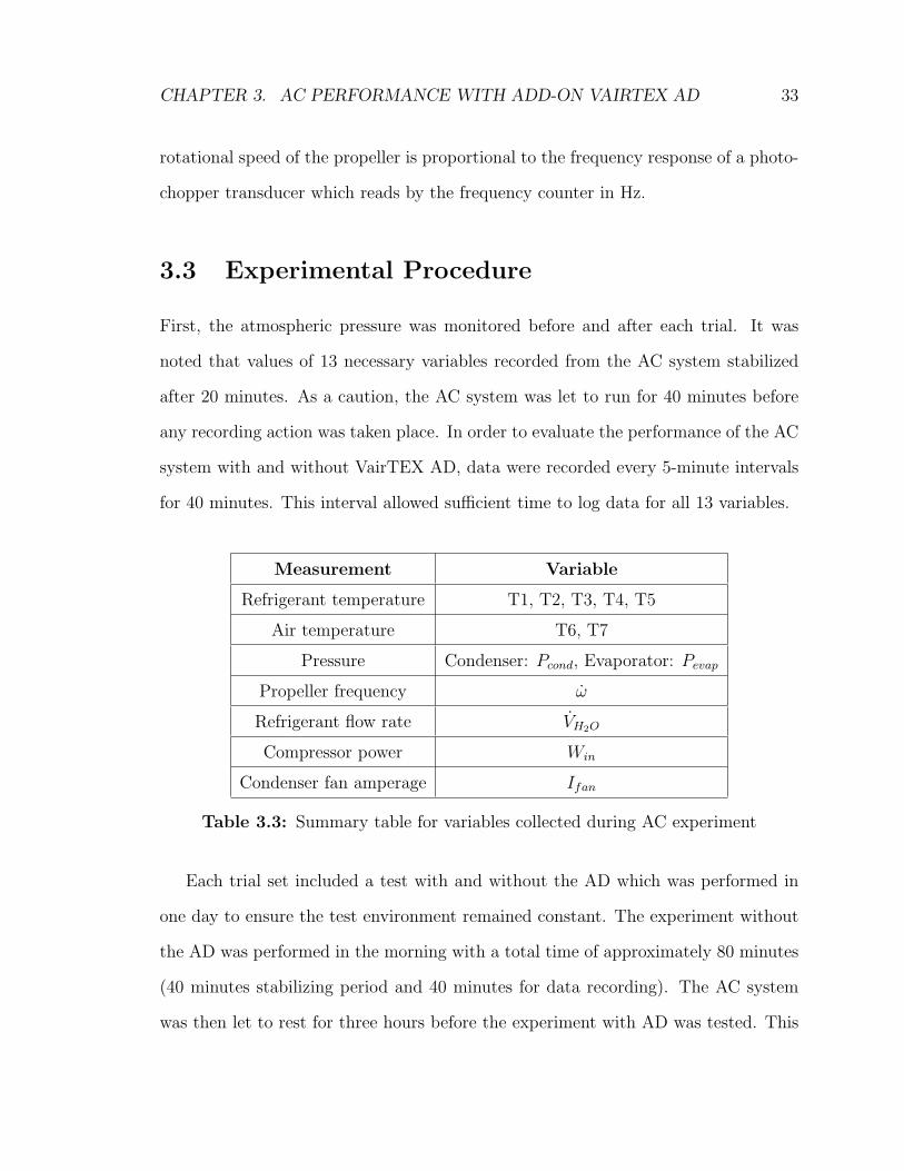
CHAPTER 3. AC PERFORMANCE WITH ADD-ON VAIRTEX AD 33
rotational speed of the propeller is proportional to the frequency response of a photo-
chopper transducer which reads by the frequency counter in Hz.
3.3 Experimental Procedure
First, the atmospheric pressure was monitored before and after each trial. It was
noted that values of 13 necessary variables recorded from the AC system stabilized
after 20 minutes. As a caution, the AC system was let to run for 40 minutes before
any recording action was taken place. In order to evaluate the performance of the AC
system with and without VairTEX AD, data were recorded every 5-minute intervals
for 40 minutes. This interval allowed sufficient time to log data for all 13 variables.
Measurement Variable
Refrigerant temperature T1, T2, T3, T4, T5
Air temperature T6, T7
Pressure Condenser: Pcond, Evaporator: Pevap
Propeller frequency ω
Refrigerant flow rate VH2O
Compressor power Win
Condenser fan amperage Ifan
Table 3.3: Summary table for variables collected during AC experiment
Each trial set included a test with and without the AD which was performed in
one day to ensure the test environment remained constant. The experiment without
the AD was performed in the morning with a total time of approximately 80 minutes
(40 minutes stabilizing period and 40 minutes for data recording). The AC system
was then let to rest for three hours before the experiment with AD was tested. This

CHAPTER 3. AC PERFORMANCE WITH ADD-ON VAIRTEX AD 34
resting period ensured that the same refrigerant temperature and conditions applied
with the AD experiment. Three trial sets were conducted on three different days for
two study cases. The following procedures were implemented for both study cases:
with and without the AD.
• Main power was turned on. Evaporator fan speed was switched to ‘Low’.
• After 2 minutes, adjusted the throttle to obtain desired refrigerant flow meter
reading (i.e 0.25 gal/min (0.95 L/min) or 0.35 gal/min (1.32 L/min)). The flow
meter should be monitored constantly throughout the steady state running
period.
• The multimeter, thermocouple meter and frequency counter were all turned on.
• The system was allowed to run for 40 minutes to reach steady state before data
was taken.
• Data of 13 variables (see Table 3.3) were recorded in sequence every 5 minutes
for 40 minutes.
For each study case, a total of 24 data points taken was output in a .txt file before
feeding into MATLAB script to evaluate performance of the AC system.
3.4 Data Reduction
Enthalpy calculations represented a time-consuming process which sometimes re-
quired double-integration. A MATLAB script was written first to resolve enthalpy
values at each measuring location. Secondly, the script was used to perform calcula-
tion following the data reduction methodology, specifically refrigeration capacity and
COP for each trial.
CHAPTER 3. AC PERFORMANCE WITH ADD-ON VAIRTEX AD 35
3.4.1 Assumption
Measuring locations are labelled in Figure 3.3. By applying the first law of ther-
modynamics, refrigeration capacity and COP are examined in order to compare the
system performance between operating with and without the VairTEX AD. A few
assumptions are made in order to make calculations possible:
1. A control volume at steady state is applied for each component in the cycle.
2. No heat transfer in connecting pipe lines since all pipes in this system were
well-insulated.
3. Neglect kinetic and potential energy changes across each component.
4. Neglect pressure drops through the condenser and evaporator. Hence
P1 = P4 = P5 = Pevaporator (3.1)
and
P2 = P3 = Pcondenser (3.2)
5. Enthalpy remains constant across the throttle or
h3 = h5 (3.3)
3.4.2 Enthalpy
Temperature and pressure measurements were used to find corresponding enthalpy
at each location, based on refrigerant R-22 and air properties provided in Table A7
and Table A22 [37].

CHAPTER 3. AC PERFORMANCE WITH ADD-ON VAIRTEX AD 36
3.4.3 Refrigeration flow rate
The flow meter provides readings on water scale, therefore, the conversion to volu-
metric flow rate of refrigerant is established in the formula below
VR22 = [(1.56 · 103) · υR22 − 0.556]1
2 · [VH2O] · [6.31 · 10−5] (3.4)
where VR22 is refrigerant volumetric flow rate [m3/s]. VH2O is reading from flow meter
[gal/min]. υR22 is the specific volume [m3/kg] of the refrigerant which is evaluated
based on temperature and pressure measured at location 3 in Figure 3.3. Hence,
the mass flow rate of the refrigerant mR22 [kg/s] can be determined by applying the
following formula:
mR22 =VR22
υR22
(3.5)
3.4.4 Air flow rate
Based on the frequency recorded from the propeller, velocity of the air stream can be
determined by the following equation
Vair = 0.294 · ω (3.6)
where ω is the rotational speed [rev/s] of the propeller.
Then the air mass flow rate at the evaporator exit can be calculated using the
expression below
mair =Vair · Aanemometer
υ6(3.7)
where Aanemometer is the cross-sectional area of the anemometer and υ6 is the specific

CHAPTER 3. AC PERFORMANCE WITH ADD-ON VAIRTEX AD 37
volume of air at the propeller anemometer.
3.4.5 Refrigeration capacity
First, as shown in Figure 3.4, a control volume is drawn around the evaporator coil.
The refrigeration capacity, denoted as Qin, is calculated as
Qin = mR22(h4 − h5) (3.8)
6
4
7
Qin
Evaporator Fan
Propeller Anemometer
Ambient Air
5
Evaporator Coil
Figure 3.4: Schematic of an evaporator unit where the dash line represents a controlvolume around the evaporator coil
3.4.6 Coefficient of performance
The COP is defined as the ratio between cooling effect over the total power input,
hence
COP =mR22(h4 − h5)
Winput
(3.9)
3.4.7 Energy efficiency ratio
In this study, the condenser was placed indoor, where temperature was kept around
20C for all measurements. The recorded data does not reflect the influence of outside
temperature on the performance of the condenser in particular and the system in

CHAPTER 3. AC PERFORMANCE WITH ADD-ON VAIRTEX AD 38
general, in evaluating seasonal energy efficiency ratio (SEER) value. Therefore, only
the energy efficiency ratio (EER) is considered in this study and can be calculated
by the ratio between cooling capacity [Btu] over total power input [W], as followed
EER =Qin ∗ 12000
Winput ∗ 1000(3.10)

Chapter 4
Hot-wire Six-Orientation Measurement
Technique
Initially particle image velocimetry (PIV) technique was used as a tool to measure
velocity at the condenser exhaust. PIV is a non-intrusive method which produces two-
dimensional or even three-dimensional vector fields. However, due to an unforeseeable
technical problem, the PIV system broke down. The available fund for this project
could not afford a replacement of a similar system. Therefore, other options had to
be explored for velocity measurement. With the availability of hot-wire anemometer
(HWA), it became an alternative method despite a disadvantage as this technique
gives velocity at a single point. Measurements from the HWA are going to be used
to explain the thermodynamic performance differences of an AC system between two
study cases: with and without the VairTEX AD.
Hot-wire anemometers have been used since the late 1800s when experimentalists
in fluid mechanics first built their own constant current anemometers [41]. As early
as 1909, Riabouchinsky, and group of Kennelly, Wright and Van Bylevelt derived the
concept of electrical anemometry. First publications on HWA design were done by
Bordoni in 1912, then by Retschy in 1913. Later years saw improvements in hot-wire
39

CHAPTER 4. HOT-WIRE SOM TECHNIQUE 40
measuring techniques, for example: in 1917, research from Fay discovered the use of
auxiliary wire to improve velocity measurement and in 1920, Thomas applied glass
coating on wire used in chemical medium [42].
Although the hot-wire anemometer is a well-known instrument for measurement
in air, it can also be used to measure flows in various mediums such as fresh water, sea
water, polymer solutions, blood, mercury, glycerine, oil and luminous gases. Hot-wire
is also used to collect measurements in different flow types for example: compressible
flows, two-phase flows or gas mixture concentrations. For turbulence flow measure-
ments, hot-wire is an ideal research tool due to its excellent frequency response - from
20-50 kHz up to 400 kHz, low signal-to-noise ratio, low-cost, wide velocity range. In
addition, hot-wire is sensitive to low velocity, has good spatial resolution, well-defined
calibration characteristics and is convenient for data analysis [43].
For heated wire type, the sensor is made from materials that are sensitive to
change in temperature such as tungsten, platinum, or platinum alloys, while the
prongs are usually made of steel or nickel. The size of wire sensors are relatively
small to minimize interference with the flow, which range from 0.25 µm to 12 µm
in diameter [43]. For measurement of fluid temperature less than 1500C, tungsten
wires are commonly used, while for high temperature velocity measurement ( 1500C
< T < 7500C), platinum and its alloys are often employed.
The most popular used hot-wire probe and the least expensive type is single-wire
sensors which are made of tungsten or platinum. These filaments have a length of 1
mm and a diameter of about 5 µm [44]. Figure 4.1 shows a typical tungsten single-wire
sensor which was made by Dantec Dynamics.


CHAPTER 4. HOT-WIRE SOM TECHNIQUE 42
4.1.1 Operational Mode
HWA can be operated in three main modes: constant temperature, constant current,
and constant voltage anemometry. The most common operation mode is the con-
stant temperature anemometer (CTA). The sensor heating current varies with the
fluid velocity to maintain constant sensor resistance, hence keep the sensor temper-
ature constant [41]. The CTA consists of a feedback amplifier, and its heart - the
Wheatstone bridge circuit, in which the hot-wire sensor acts as one resistor in the
circuit, as illustrated in Figure 4.2
Servo
Amplifier
Top of Bridge
R1R2
Null resistance
Resistance decade
R3Rprobe
Eb
Figure 4.2: Wheatstone bridge circuit in a constant temperature anemometer oper-ation mode where hot-wire probe acts as one of the resistors in the bridge. Adaptedfrom AA Lab Systems Ltd. [46]
Change in flow velocity causes change in heat transfer rate and sensor resistance,
and thus cause the wire to cool off or heat up. As this happens, the Wheatstone bridge
becomes unbalanced. The differential feedback amplifier detects the imbalance and
adjusts the current flowing to the sensor in order to return the bridge to balance
mode. Since the feedback amplifier response time is short, the thermal inertial effect
CHAPTER 4. HOT-WIRE SOM TECHNIQUE 43
can be neglected and the sensor temperature always remains constant [41, 47]. The
output voltage across the bridge, seen by the feedback amplifier, is proportional to the
fluid velocity. Hence the indication of magnitude and instantaneous velocity vector
are provided through the wire.
4.1.2 Response Equation
The output voltage E of the hot-wire and flow velocity U are followed by a non-linear
relationship. The response equation was derived by King (1914), given as
E2 = A+BUn (4.1)
where A, B and C are calibration constants. King suggested that n = 0.5 for a limited
range of velocity [47] while studies from Van Thinh (1969), Bruun (1976), Bruun and
Tropea (1980, 1985), Swaminathan et al. (1983) and Pitts and McCaffrey (1986)
have demonstrated the optimum value of n for 5 µm tungsten hot-wire ranges from
0.4 to 0.45 for moderate velocity range (i.e. from 5 - 60 m/s) [48]. An approach
from Davies and Patrick (1972) and Siddall and Davies (1972) shown an excellent fit
for a calibration curve over a large range of velocity, from 1 - 60 m/s [49], using an
extended power law in the form
E2 = A+BU0.5 + CU (4.2)
In one dimensional flow, the wire is placed perpendicular to the mean velocity,
hence the output voltage of the HWA represents the true velocity, also known as the
effective cooling velocity through Equation 4.3. When the wire is placed in three
dimensional flow, the components of turbulence affect the instantaneous velocity seen
by the wire. Hence, it is necessary to express the effective cooling velocity Z in terms

CHAPTER 4. HOT-WIRE SOM TECHNIQUE 44
of all three orthogonal velocity components u, v and w. The relationship is derived
by Jorgensen [50] as follows
Z2 = v2 +G2u2 +K2w2 (4.3)
where G and K are referred to pitch and yaw factors.
According to Jorgensen, the pitch factor is defined as the ratio between the sen-
sitivity of v component to the sensitivity of u component, as shown in Equation 4.4;
whereas the yaw factor is defined as the fraction between the sensitivity of v compo-
nent to w component, as described in Equation 4.5 , for a constant voltage square
(E2).
G =v
u(4.4)
and
K =v
w(4.5)
with u, v and w components are obtained at zero velocity in the other two directions.
4.2 Multi-Position Measuring Techniques
Having obtained the calibration procedure for the HWA, it is now necessary to deter-
mine the best method to solve three velocity components. Turbulence measurement
of a complex flow field has always been a challenge for engineers and physicists. A sin-
gle hot-wire can be used to measure the time-mean velocity and the root-mean-square
of the streamwise components in one-dimensional flow. A double wire probe is able
to determine the time-mean velocities of the streamwise and cross stream turbulence
CHAPTER 4. HOT-WIRE SOM TECHNIQUE 45
intensities, and also the cross correlation between the two components of the velocity
fluctuations [51–53]. In the case of a three-dimensional flow field, the velocity compo-
nents and their corresponding fluctuations require a minimum of three simultaneous
equations and can be solved by implementing either of the two following methods:
1. A multi-wire probe placed at a single orientation.
2. A single-wire probe placed at multi-orientation.
The multi-wire method employs three-wire probe which permits simultaneous
reading of three response equations since all three wires lie within the same vol-
ume of the flow field. These equations must be expressed in form of the effective
cooling velocity. However, the multi-wire probe technique faces several drawbacks,
such as:
1. Three-wire probe requires three identical or closely matched anemometer units.
2. It produces significant aerodynamic prong interference unless each sensor is
placed at a certain spatial offset, or the probe is orientated relative to the mean
velocity and turbulence intensity is low.
3. Thermal-wake interference from one wire to another can generate spurious read-
ings.
Dvorak and Syred [54] derived a method using a single normal hot-wire rotated at
three different positions which were separated by 45 from each other. The velocity
vector was decomposed into three orthogonal components using pitch and yaw factors
as defined above by Jorgensen. However, with this method, information from the
measurement was insufficient to obtain the quantities of turbulence. Hence, Dvorak
and Syred introduced the use of a cross-wire probe to obtain the covariances between
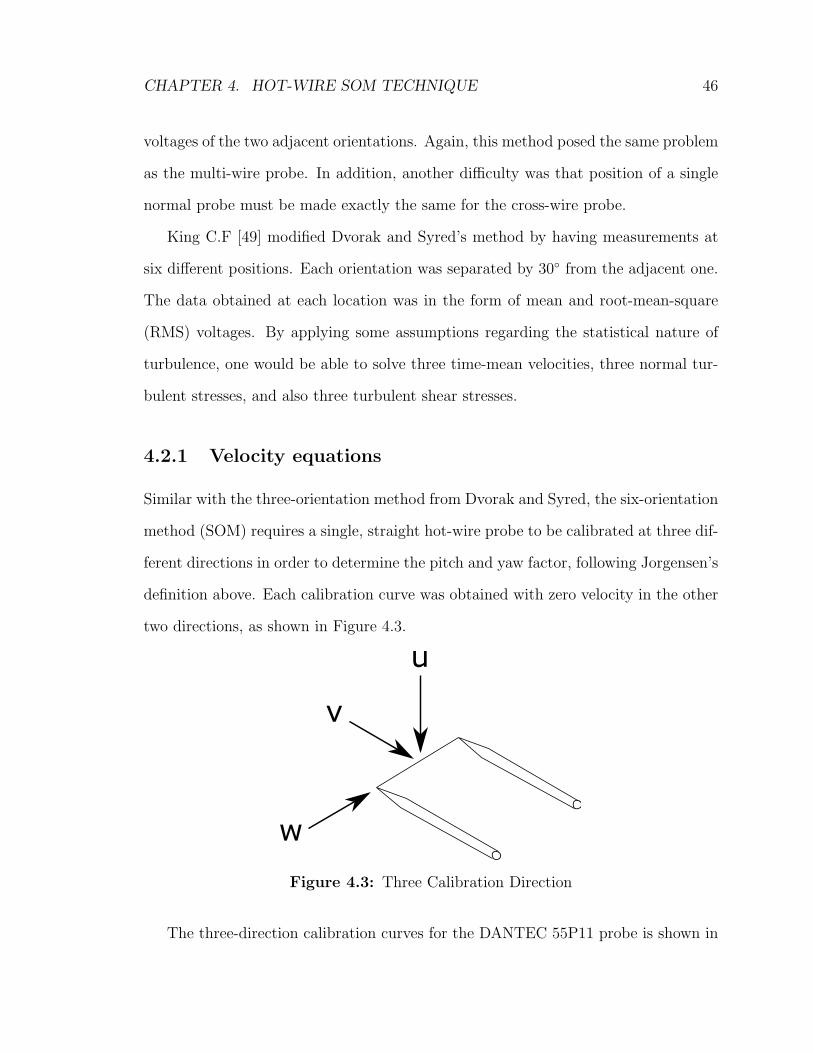
CHAPTER 4. HOT-WIRE SOM TECHNIQUE 46
voltages of the two adjacent orientations. Again, this method posed the same problem
as the multi-wire probe. In addition, another difficulty was that position of a single
normal probe must be made exactly the same for the cross-wire probe.
King C.F [49] modified Dvorak and Syred’s method by having measurements at
six different positions. Each orientation was separated by 30 from the adjacent one.
The data obtained at each location was in the form of mean and root-mean-square
(RMS) voltages. By applying some assumptions regarding the statistical nature of
turbulence, one would be able to solve three time-mean velocities, three normal tur-
bulent stresses, and also three turbulent shear stresses.
4.2.1 Velocity equations
Similar with the three-orientation method from Dvorak and Syred, the six-orientation
method (SOM) requires a single, straight hot-wire probe to be calibrated at three dif-
ferent directions in order to determine the pitch and yaw factor, following Jorgensen’s
definition above. Each calibration curve was obtained with zero velocity in the other
two directions, as shown in Figure 4.3.
v
u
w
Figure 4.3: Three Calibration Direction
The three-direction calibration curves for the DANTEC 55P11 probe is shown in
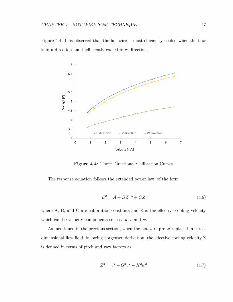
CHAPTER 4. HOT-WIRE SOM TECHNIQUE 47
Figure 4.4. It is observed that the hot-wire is most efficiently cooled when the flow
is in u direction and inefficiently cooled in w direction.
3
3.5
4
4.5
5
5.5
6
6.5
7
0 1 2 3 4 5 6 7
Vo
lta
ge
[V
]
Velocity [m/s]
U direction V direction W direction
Figure 4.4: Three Directional Calibration Curves
The response equation follows the extended power law, of the form
E2 = A+BZ0.5 + CZ (4.6)
where A, B, and C are calibration constants and Z is the effective cooling velocity
which can be velocity components such as u, v and w.
As mentioned in the previous section, when the hot-wire probe is placed in three-
dimensional flow field, following Jorgensen derivation, the effective cooling velocity Z
is defined in terms of pitch and yaw factors as
Z2 = v2 +G2u2 +K2w2 (4.7)

CHAPTER 4. HOT-WIRE SOM TECHNIQUE 48
Since calibration curves in v direction are closer to the one in u direction than
in w direction, the yaw factor is more sensitive to voltage fluctuation than the pitch
factor. The pitch and yaw factors will be evaluated from the three calibration curves
at a constant E2 value.
To characterize a three dimensional flow field, three means and RMS velocity
components are generally required. In order to solve six unknowns, six equations
need to be obtained. A hot-wire probe is rotated six times around the probe axis
where each position is spaced 30 from each other, as shown in Figure 4.5. Due to the
inability to distinguish between positive and negative directions, the positions have a
circularity characteristic, meaning same reading is shared between positions 1 and 6.
12
3
4
5
6
300
Figure 4.5: Six positions of measurement for single hot-wire probe
The measurement at first position is carried out where the wire is normal to the
axial direction of the flow, and the probe coordinates coincide with the flow field
coordinate system. As the probe rotates from position 1 to 6, the effective cooling
velocity equation for six positions, as given by King [55]are

CHAPTER 4. HOT-WIRE SOM TECHNIQUE 49
Z21 = V 2 +G2U2 +K2W 2 (4.8)
Z22 = V 2 +G2(Ucos300 +Wsin300)2 +K2(Wcos300 − Usin300)2 (4.9)
Z23 = V 2 +G2(Ucos600 +Wsin600)2 +K2(Wcos600 − Usin600)2 (4.10)
Z24 = V 2 +G2W 2 +K2U2 (4.11)
Z25 = V 2 +G2(Ucos1200 +Wsin1200)2 +K2(Usin1200 −Wcos1200)2 (4.12)
Z26 = V 2 +G2(Ucos1500 +Wsin1500)2 +K2(Usin1500 −Wcos1500)2 (4.13)
Solving any three adjacent equations simultaneously provides expressions for the
instantaneous values of three velocity components U, V and W in terms of the equiv-
alent effective cooling velocities. A general solution for three velocity components U,
W, and V is denoted as F1, F2, F3 where the value of AO, BO, and CO depend on
the set of the three equations chosen.
F1 =
√
[
AO +
√
AO2 +BO2
3
]
∗
(
1
G2 −K2
)
(4.14)
F2 =
√
[
− AO +
√
AO2 +BO2
3
]
∗
(
1
G2 −K2
)
(4.15)
F3 =
√
CO −
(
G2 +K2
G2 −K2∗
√
AO2 +BO2
3
)
(4.16)
The value of variable AO, BO, and CO are given in Table 4.1.

CHAPTER 4. HOT-WIRE SOM TECHNIQUE 50
Equation Set AO BO CO
1,2,3 Z22 − Z2
3 −2Z21 + 3Z2
2 − Z23 Z2
1 − Z22 + Z2
3
2,3,4 Z22 − Z2
3 −Z22 + 3Z2
3 − 2Z24 Z2
2 − Z23 + Z2
4
3,4,5 Z33 − 2Z2
4 + Z25 Z2
3 − Z25 Z2
3 − Z24 + Z2
5
4,5,6 −Z25 + Z2
6 −2Z24 + 3Z2
5 − Z26 Z2
4 − Z25 + Z2
6
5,6,1 −Z25 + Z2
6 −Z25 + 3Z2
6 − 2Z21 Z2
5 − Z26 + Z2
1
6,1,2 −Z26 + 2Z2
1 − Z22 −Z2
6 + Z22 Z2
6 − Z21 + Z2
2
Table 4.1: AO, BO, and CO values for corresponding equation set
Following Janjua [56] and King [49] Fortran code, the equation set was chosen
with respect to the minimum effective velocity. For example, if the minimum effective
velocity Z was located at position 4, the equation set would be chosen as 3, 4, and
5. Six response equations 4.8 to 4.13 and the general expressions for U, W, and V
are all in terms of instantaneous velocity. Moreover, it is impossible with a single
hot-wire to obtain any set of three equations (i.e Z1, Z2, Z3) at a single instant in
time. Therefore, equations F1, F2, and F3 must be time-mean. In order words, they
must be expressed in terms of mean and root-mean-square values.
4.2.2 Statistical analysis
A statistical method to establish time averaged velocities has been adopted from
Dvorack and Syred with the assumption that the turbulence is stationary [54]. This
assumption is necessary for any orientation technique since the turbulence must re-
main the same while the probe is placed into the flow. In a fully developed flow where
there is no variation with time, this assumption seems to be reasonable. First, the
instantaneous effective cooling velocity Zi can be written in term of a function φ of
an instantaneous voltage Ei by rearranging Equation 4.6.

CHAPTER 4. HOT-WIRE SOM TECHNIQUE 51
φ(Ei) = Zi =
[
−B +√
B2 − 4C(A− E2i )
2C
]2
(4.17)
Then, in order to obtain an expression for time-mean velocity of each individual
position Zi as a time-mean voltage, a Taylor series expansion of Equation 4.17 is
carried out.
Since Zi = φ(Ei + E ′
i)
Zi = φ(Ei + E ′
i) = φ(Ei) +E ′
i
1!·∂φ
∂Ei
+(E ′
i)2
2!·∂2φ
∂E2i
(4.18)
The Taylor series is truncated after second order term due to those high order
terms which are relatively small in comparison with the first and second terms. Time
averaging both sides of Equation 4.18 and taking into account the fact that E ′
i = 0 [57]
to obtain
Zi = φ(Ei) +1
2
∂2φ
∂E2i
· σ2Ei
(4.19)
Equation 4.19 is evaluated with mean voltage Ei and the σ2Ei
is taken the value
of the square RMS voltage.
Second, to evaluate the fluctuation term σ2Zi, Hinze’s relationships [58] are used
Z ′
i
2= σ2
Zi= Expec[Z2
i ]− (Expec[Zi])2 (4.20)
The first part of Equation 4.20 can be approximated as
Expec[Z2i ] = φ2 +
1
2
∂2φ2
∂E2i
· σ2Ei
(4.21)

CHAPTER 4. HOT-WIRE SOM TECHNIQUE 52
The differential in Equation 4.21 can be evaluated as
∂2φ2
∂E2i
=∂
∂Ei
·
(
2φ ·∂φ
∂Ei
)
= 2
(
∂φ
∂Ei
)2
+ 2φ ·∂2φ
∂E2i
(4.22)
Substituting Equation 4.22 into Equation 4.21 to obtain
Expec[Z2i ] = φ2 +
∂φ
∂Ei
· σ2Ei
+ φ ·∂2φ
∂E2i
· σ2Ei
(4.23)
The second part of Equation 4.20 is obtained by squaring Equation 4.19
(Expec[Zi])2 = φ2 +
(
1
2
∂2φ
∂E2i
· σ2Ei
)2
+ φ ·∂2φ
∂E2i
· σ2Ei
(4.24)
Finally, the variance of individual effective cooling velocity σ2Zi
is reduced to
Z ′
i
2= σ2
Zi=
(
∂φ
∂Ei
)2
· σ2Ei
−
(
1
2
∂2φ
∂E2i
· σ2Ei
)2
(4.25)
Equation 4.19 and 4.25 provide the mean and variance of individual cooling ve-
locities in terms of mean and variance of the according voltage. It is now possible to
solve the three instantaneous velocity components U, V and W in term of mean and
variance individual cooling velocities.
In a three-dimensional flow, besides mean and variance values expressed in each
velocity component equation, it is also required their cross correlations. The proce-
dure to obtain the mean and variance of the individual velocity components is similar
to the effective cooling velocities except that U, V and W are functions of three ran-
dom variables and there are extra terms in the Taylor expansion to account for the
covariances of the effective cooling velocities. Thus the three mean velocities are given
by

CHAPTER 4. HOT-WIRE SOM TECHNIQUE 53
U = F1 +1
2
3∑
i=1
∂2F1
∂Z2i
· σ2Zi
+3
∑
i<j
∂2F1
∂Zi∂Zj
·KZiZj(4.26)
and
W = F2 +1
2
3∑
i=1
∂2F2
∂Z2i
· σ2Zi
+3
∑
i<j
∂2F2
∂Zi∂Zj
·KZiZj(4.27)
and
V = F3 +1
2
3∑
i=1
∂2F3
∂Z2i
· σ2Zi
+3
∑
i<j
∂2F1
∂Zi∂Zj
·KZiZj(4.28)
where KZiZjis the covariance of the effective cooling velocity fluctuations and is
defined as
KZiZj=
1
t
∫ t
0
(Zi − Zi)(Zj − Zj)dt (4.29)
4.2.3 Covariance
King devised a mathematical procedure to calculate the covariances in his study of a
vortex amplifier. The detail of this method can be found in his Ph.D thesis [49]. The
covariances are calculated based on the relationship
KZiZj= γZiZj
(σ2Zi
· σ2Zj)0.5 (4.30)
where γZiZjis the correlation coefficient between the two cooling velocities Zi and Zj.
The covariances for two 30 wire separation are denote as KZPZQ, KZQZR
, while the
covariances for 60 separation is written as KZPZR. In case the covariance values are
bigger than one, King fixed the values of the correlation coefficients as
γZPZQ= 0.9 γZQZR
= 0.9 γZPZR= 0.648 (4.31)

CHAPTER 4. HOT-WIRE SOM TECHNIQUE 54
In Janjua’s work [56], he discovered that in case of turbulence measurement in
a confined jet using the six-orientation technique, King’s estimate of the covariances
was not self-consistent. Therefore, Janjua employed those fixed values for correlation
coefficients to calculate the covariances.
The first two values γZPZQand γZQZR
are estimated based on the fact that if two
consecutive measuring positions are separated by an angle of 30, then the contribu-
tion of fluctuating signals from each hot-wire measurement position to the effective
cooling velocity of the wire is related by the cosine value of that angle. Hence,
γZPZQ= cos 30 = 0.87 ≈ 0.9 and γZQZR
= cos 30 = 0.87 ≈ 0.9. For the correlation
coefficient where the two wires are set apart by 60 , γZPZRis related to the other
correlation coefficients by the expression below as
γZPZR= η · γZPZQ
· γZQZR(4.32)
If η takes the value of 0.8, then
γZPZR= 0.8 · 0.9 · 0.9 ≈ 0.648 (4.33)
which is close to the value of cos 60. Therefore the cosine relationship still holds in
case of 60 wire separation if η = 0.8.
Three covariances are evaluated by substituting the corresponding values of the
correlation coefficients into Equation 4.30. For the analysis in this thesis, since the
flow at the condenser exit resembles the flow in the axisymmetric combustor of a gas
turbine engine more than in the vortex amplifier’s case, the estimate of correlation
coefficients and the procedure to obtain covariances follow Janjua’s work.

CHAPTER 4. HOT-WIRE SOM TECHNIQUE 55
4.2.4 Coordinate system
The hot-wire probe was placed at the condenser exit such that at position 1, the
hot-wire coordinate coincide with the velocity components of the flow field U, V, and
W where:
U = Radial Velocity Component
V = Axial Velocity Component
W = Tangential Velocity Component
v
uw
U
V
W
Condenser
Figure 4.6: Hot-wire probe coordinate u, v, and w at position 1 in related to flowfield coordinate system U, V and W
Relative to the hot-wire coordinate system, Figure 4.6 shows the positive direction
of U, V, and W that will be applied in the data reduction analysis for SOM method.
4.3 Calibration Setup
Calibration was initially performed at the atmospheric boundary layer wind tunnel
situated in room ME 2140 at Carleton University. However, the lowest operation
speed in the wind tunnel was approximately 3.3 m/s which was higher than some

CHAPTER 4. HOT-WIRE SOM TECHNIQUE 56
of the measuring points expected in the flow field at the condenser exit (where flow
could be as low as 0.5 m/s). McTavish implemented a series of sandwiched screens
which were placed upstream of the test section in order to reduce the wind speed.
Despite this attempt, the speed was only brought down to 2 m/s [59]. Therefore,
there was a strong need for constructing a calibration facility that could produce flow
as low as 0.5 m/s.
A simple, inexpensive, easily built calibration facility, following Grandchamp’s
design [60, 61] of a ‘desktop’ wind tunnel was created for the calibration process of
the hot-wire in three different directions. All components were set up in a series.
The facility consisted of a 1/4′′ Power First diaphragm-type pressure regulator, with
maximum pressure of 160 psi (1,103 kPa), to control the flow from the compress air
line. The regulator was then connected to the Brooks Mass Flow Meter 5863S, via a
uniform stainless steel duct of diameter 0.0096 m. The air was then passed through
another stainless steel duct of the same diameter before entering the building-block
of the ‘desktop’ wind tunnel which comprised of:
1. A diffuser
2. A settling chamber
3. A contraction nozzle
The diffuser and contraction nozzle were printed using the Dimension BST three-
dimensional printer available in the department. The following descriptions outline
the process of designing the main portion of the ‘desktop’ wind tunnel.
The diffuser is basically an expansion duct to reduce flow velocity in order to
convert kinetic energy into pressure energy as efficiently as possible [62]. The area

CHAPTER 4. HOT-WIRE SOM TECHNIQUE 57
L
D1D2
θ
Figure 4.7: General geometry of diffuser section where D1 is throat diameter, D2 isexit diameter, L is diffuser length and θ is conical angle.
of the diffuser should increase gradually to prevent flow separation [63]. General
geometry of the diffuser is shown in Figure 4.7.
Mehta’s study indicated that the conical angle for a diffuser should be between
5 (for best flow steadiness) and 10 (for best pressure recovery) [64]. Thus it makes
sense that general practice used cone angle of 7 for the diffuser [65, 66]. This angle
was applied to the geometry of the diffuser in this setup. Besides the conical angle,
two other factors dictate the performance of a conical diffuser are area ratio A2/A1,
and length-to-throat diameter ratio L/D1. The area ratio of the diffuser is the ratio
between the cross section of the stainless pipe and the PVC pipe which was around
17 in this setup. According to the performance data of a conical diffuser provided
by Runstadler Jr. et al. [67], for conical angle of 7 and area ratio of 17, the length-
to-throat diameter ratio is approximately 13 which result in diffuser length of 0.165
m.
A straight PVC pipe, separating the diffuser from the nozzle, acted a settling
chamber to ensure total flow mixing. For internal incompressible viscous flow, the
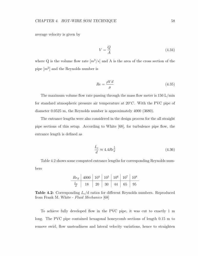
CHAPTER 4. HOT-WIRE SOM TECHNIQUE 58
average velocity is given by
V =Q
A(4.34)
where Q is the volume flow rate [m3/s] and A is the area of the cross section of the
pipe [m2] and the Reynolds number is
Re =ρV d
µ(4.35)
The maximum volume flow rate passing through the mass flow meter is 150 L/min
for standard atmospheric pressure air temperature at 20C. With the PVC pipe of
diameter 0.0525 m, the Reynolds number is approximately 4000 (3680).
The entrance lengths were also considered in the design process for the all straight
pipe sections of this setup. According to White [68], for turbulence pipe flow, the
entrance length is defined as
Le
d≈ 4.4Re
1
6
d (4.36)
Table 4.2 shows some computed entrance lengths for corresponding Reynolds num-
bers
Red 4000 104 105 106 107 108
Le
d18 20 30 44 65 95
Table 4.2: Corresponding Le/d ratios for different Reynolds numbers. Reproducedfrom Frank M. White - Fluid Mechanics [68]
To achieve fully developed flow in the PVC pipe, it was cut to exactly 1 m
long. The PVC pipe contained hexagonal honeycomb sections of length 0.15 m to
remove swirl, flow unsteadiness and lateral velocity variations, hence to straighten

CHAPTER 4. HOT-WIRE SOM TECHNIQUE 59
the flow [69] before it entered the nozzle section. Both ends of PVC pipe sections
were equipped with flanges in order to align with the flanges from the diffuser and
nozzle sections. Also, all 0.0096 m diameter stainless steel pipe sections had a length
of 0.04 m which well ensured fully developed flow in these pipe sections.
Convergent nozzle is a device that is used to accelerate the flow and also provides
uniform velocity profile at the exit. The geometry of the contraction shape is shown
in Figure 4.8.
Match Point
L
R1
R2
xm
Figure 4.8: Schematic of the convergent nozzle with matched fifth order polynomialwhere R1 and R2 is are inlet and exit radii, L is the total length, xm is the distancefrom the inlet to the match point where the two polynomials of same curvature andslope meet [70]
The nozzle section followed Morel’s contraction design criteria [71] due to its
simplicity and effectiveness. Moreover, this method considered uniform flow at the
exit as being the basic requirement in the design process, which was also the desired
achievement in this setup. The criteria are listed below as
0.75 ≤ L/D1 ≤ 1.25
0.2 ≤ xm/L ≤ 0.8
2 ≤ CR ≤ 25

CHAPTER 4. HOT-WIRE SOM TECHNIQUE 60
The inlet diameter of the nozzle had a dimension as the straight PVC pipe while
the exit diameter had a value of 0.018 m to produce a maximum velocity of approx-
imately 10 m/s (based on maximum flow rate of 150 L/min). The contraction area
ratio (CR) is then restricted to a value of 8.5 in this design. Based on the criteria
above, the ratio L/D1 was chosen to be 1.25 while ratio xm/L was selected as 0.55.
Hence the total length L of the nozzle was 0.0656 m. As recommended by Su, the
contraction section after the settling chamber should follow a polynomial higher than
3 order [72]. In this case, the nozzle shape profile followed a fifth order polynomial
with R-squared equals to 0.999. Schematic of the mini wind tunnel used to perform
calibration is illustrated in Figure 4.9.
Air
Regulator
Flow
meter Diffuser
Honeycomb
structure
Straight
PVC pipeNozzle
Metal
pipeCompressed
air line
Flange
Flange
Hotwire
Probe Traverse
system
400
mm
165
mm65.6
mm1000
mm
400
mm
Metal
pipe
Figure 4.9: Schematic of a mini-version wind tunnel where calibrations in threedirections were performed
4.4 Temperature Correction
For a CTA operation mode of hot-wire, one of the most significant sources of error
needed to take into account, is the changes in velocity reading due to changes in
ambient temperature. Generally speaking, the hot-wire should be calibrated and
operated at the same temperature. In practice, if the temperature changes within ±
0.5C throughout calibration and measurement, it is not necessary to proceed with

CHAPTER 4. HOT-WIRE SOM TECHNIQUE 61
any correction [73]. However, when the fluctuation is greater than 0.5C, a correction
must be performed.
Preliminary measurements showed temperatures at the condenser exit were dif-
ferent from calibration temperature and they also varied in a range of approximately
10C. Hence a temperature correction method must be used to minimize voltage
drifting due to a temperature difference between calibration and measurements. Nu-
merous techniques, based on the assumption of King’s heat transfer law, have been
developed by Collis and Williams [74], Grant and Kronauer [75], Bearman [76], Abdel-
Rahman and Strong [77], Benjamin and Roberts [78], and the most recent by Tropea
et al. [79]. But these techniques are cumbersome and inconvenient to incorporate
in the data analysis. The most commonly used technique, derived by Brunn [43],
is correcting the output voltage Ew based on a reference temperature Tr (usually
corresponding to the calibration temperature) in the form of
Ew,r = Ew
[
Tw − Tr
Tw − Ta
]0.5
(4.37)
where Tw and Ta are wire and ambient temperatures while Ew,r is voltage corrected.
However, this method is only valid up to a drift of 3C from the calibration temper-
ature. A new correction scheme for the CTA mode presented by Hultmark [80] is
examined. This method requires a minimal of additional calibration, it is not based
on an assumed heat transfer law, and is simple to apply in the data analysis. Most
importantly, Hultmark’s correction method works effectively for a large range of el-
evated temperature of up to 15C in the CTA mode. The detail of this method is
described below.
Resistance and temperature of the sensor follows Hinze’s relationship [58] as
Rs = Ro[1 + α(Ts − To) + α1(Ts − To)2 + ...] (4.38)

CHAPTER 4. HOT-WIRE SOM TECHNIQUE 62
where T and R stand for temperature and resistance. Two subscripts s and o rep-
resent sensor and reference values. α is the temperature coefficient of resistivity.
Typical sensor materials such as platinum or tunsten, α ≥ α1, then the Equation
4.38 is reduced to
Rs = Ro[1 + α(Ts − To)] (4.39)
An important factor when analyzing the heat transfer of the wire is the aspect
ratio (AS) which is defined as
AS =l
d(4.40)
where l is the length of the wire and d is its diameter. Dantec single hot-wire probe
55P11 has an AS of 250 [81]. According to Perry and Bruun [43, 73], for wire with
AS ≥ 200, the end-conduction effects can be neglected. Also, the analysis considers
only forced convection and excludes free convection effect. In CTA operation mode,
the wire resistance is kept constant through the expression
E2
R= h∆TA =
kNu
dA∆T (4.41)
where h is the convection heat transfer coefficient, k is the thermal conductivity of
the fluid, ∆T = Tw − Ta, A is the surface area of the wire, and Nusselt number
Nu = hd/k. In subsonic flow, the Nusselt number depends on both Reynolds number
Re and Prandtl number Pr [82]. However, we can assume that Nu = f(Re) only as
Prandtl number is a weak function of temperature. For a given wire, d, A, and R are
constant, thus Equation 4.41 can be rewritten as
E2 = f(Re)k∆T (4.42)
CHAPTER 4. HOT-WIRE SOM TECHNIQUE 63
Rearranging Equation 4.42 to obtain Re as
Re = f2
(
E2
k∆T
)
(4.43)
or
V
ν= f2
(
E2
k∆T
)
(4.44)
where f2 denotes an inverse function. Since ν and k are functions of temperature,
the corrected velocity can now be determined based on the recorded voltage. The
thermal conductivity of air, evaluated at film temperature of Tf = 0.5 · (Tw + Ta), is
found using the correlation given by Kannuluik and Carman [83] as
k = 418.4 · [5.75× 10−5(1 + 0.00317 · Tf − 0.0000021 · Tf2)] (4.45)
While the kinematic viscosity ν of air can be found using the relation provided by
Dixon [84] where
ν =1.458× 10⁻⁶(273.15 + T )1.5
ρ[(273.15 + T ) + 110.4](4.46)
where ρ is the density of air at the corresponding temperature T in Celsius degree.
Figure 4.10 (a) shows calibration curves obtained in Hultmark’s study at differ-
ent temperatures while (b) demonstrates the effectiveness of applying his correction
method for the CTA operation mode.

CHAPTER 4. HOT-WIRE SOM TECHNIQUE 64
3
4
5
6
7
8
9
6.4 6.6 6.8 7 7.2 7.4 7.6 7.8 8 8.2
Ve
loci
ty [
m/s
]
Voltage [V]
48 Degrees
45 Degrees
39 Degrees
33 Degrees
(a)
0.00E+00
1.00E+05
2.00E+05
3.00E+05
4.00E+05
5.00E+05
6.00E+05
7.00E+05
8.00E+05
10 12 14 16
U/ν
E2/kΔT
48 Degrees
45 Degrees
39 Degrees
33 Degrees
(b)
Figure 4.10: CTA mode calibration and correction curves from Hultmark’s study. (a) Original calibration curves at different temperatures and (b) Curves replottedusing similarity variable given by Equation 4.44. Reproduced from Ref [80]
To validate this method, calibration curves at different temperatures were collected
by using the in-house ‘desktop’ wind tunnel on different days. The data were taken
using Dantec single miniature probe 55P11, operated at wire temperature of 86C.
0
1
2
3
4
5
6
7
3 3.2 3.4 3.6 3.8 4 4.2 4.4 4.6 4.8 5 5.2 5.4 5.6
Ve
loci
ty [
m/s
]
Voltage [V]
33 Degrees
28.6 Degrees
23.8 Degrees
20 Degrees
(a)
0.00E+00
1.00E+05
2.00E+05
3.00E+05
4.00E+05
5.00E+05
6 8 10 12 14 16 18
U/ν
E2/kΔT
33 Degrees
28.6 Degrees
23.8 Degrees
20 Degrees
(b)
Figure 4.11: (a) In-house calibration curves at different temperatures and (b) Curvesreplotted following Hultmark’s correction method

CHAPTER 4. HOT-WIRE SOM TECHNIQUE 65
As seen in Figure 4.11 (a), calibration curves at four different temperatures col-
lapse to a single curve of fourth order polynomial with an R2 factor of 0.9988. This
demonstrates that Hultmark’s technique captures the effects of temperature on the
calibration process accurately and effectively.
4.5 Experimental Setup
The following section will describe in details experimental set-up for HWA measure-
ments, as well as temperature measurements at the condenser exhaust.
4.5.1 Hot-wire measurement
Six-axis rotation device
In order to collect measurements at six orientations, a special device was designed to
fulfill this task. Being machined at our Machine Shop, the SOM device consisted of
four main parts: main body, mini ball-bearing, circular rotating disk, and straight
hollow tube. Figure 4.12 illustrates the measuring device that was used to record the
HWA data. The description for each individual part is described below.
The main body outfitted of five features:
• A 5.0′′ x 2.5′′ (127.0 x 63.5 mm) plate and of thickness 0.21′′ (5.33 mm)
• An extruded support block acting as a guide for the hollow tube
• Two levels placed orthogonally on the plate body
• An L-bracket to be attached to the traverse system
• Twelve holes positioned in a circular pattern where each hole departed from the
other by 30
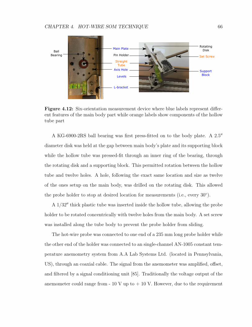
CHAPTER 4. HOT-WIRE SOM TECHNIQUE 66
Main Plate
Pin Holder
Straight
Tube
Levels
L-bracket
Support
Block
Set Screw
Rotating
Disk
Axis Hole
Ball
Bearing
Figure 4.12: Six-orientation measurement device where blue labels represent differ-ent features of the main body part while orange labels show components of the hollowtube part
A KG-6900-2RS ball bearing was first press-fitted on to the body plate. A 2.5′′
diameter disk was held at the gap between main body’s plate and its supporting block
while the hollow tube was pressed-fit through an inner ring of the bearing, through
the rotating disk and a supporting block. This permitted rotation between the hollow
tube and twelve holes. A hole, following the exact same location and size as twelve
of the ones setup on the main body, was drilled on the rotating disk. This allowed
the probe holder to stop at desired location for measurements (i.e., every 30).
A 1/32′′ thick plastic tube was inserted inside the hollow tube, allowing the probe
holder to be rotated concentrically with twelve holes from the main body. A set screw
was installed along the tube body to prevent the probe holder from sliding.
The hot-wire probe was connected to one end of a 235 mm long probe holder while
the other end of the holder was connected to an single-channel AN-1005 constant tem-
perature anemometry system from A.A Lab Systems Ltd. (located in Pennsylvania,
US), through an coaxial cable. The signal from the anemometer was amplified, offset,
and filtered by a signal conditioning unit [85]. Traditionally the voltage output of the
anemometer could range from - 10 V up to + 10 V. However, due to the requirement
CHAPTER 4. HOT-WIRE SOM TECHNIQUE 67
from the statistical analysis in Equation 4.17 where all anemometer voltage values
E needed to be either positive or negative, to prevent double roots in the solution.
Hence, the anemometer output voltage was set between 0 V and +10 V. The analog
data from the anemometer was acquired by a National Instrument Data Acquisition
(DAQ) 14-bit NI USB-6009 through a coaxial cable.
Traverse system
Aluminium T-slot beams purchased from CPI Automation Ltd. (Ontario, Canada)
with square cross-section of size 2.54 x 2.54 cm ( 1 x 1 in) were used to construct
the 1D-traverse system. To perform hot-wire measurement, a fixed frame was built
around the condenser where its fan centre of rotation was 1.24 m away from the wall
and coincided with the centre of the frame. Sitting parallel to the condenser and the
Air Director exit surfaces, the traverse beam was supported by two T-slot beam on
both sides. A timing belt was installed along the whole length of the traverse beam.
The probe system was fixed on the moving plate which was attached to the belt. This
allowed manual translation in one direction for the probe system which consisted of
the six-axis rotation device, the probe holder and the hot-wire probe.
Figure 4.13 provides an illustration of the setup for case with the VairTEX AD
added on top of the condenser unit. It should be noted that the measuring line was
offset from the exit surface of the air director by a distance of 1 cm. For measurement
without the AD, the traverse beam was lowered down and distance from the traverse
beam to the measuring line, and distance from the measuring line to the condenser
exit surface remained the same.

CHAPTER 4. HOT-WIRE SOM TECHNIQUE 68
140
132
122
114 Probe system
Air
director
Condenser
35 Measuring
line
55
30.5
58.4
Traverse beam
Figure 4.13: Schematic of a 1D traverse system surrounding the condenser unit inroom ME2230-30 at Carleton University. Note that all dimensions are in cm
A close-up view of the measuring lines for two study cases is shown in Figure
4.14. In the case without the AD applied on the condenser, a line of measurement at
the condenser discharge contained 19 points which were placed symmetrically around
the centre rotation of the condenser fan. While in the case with the AD added on,
a total of 11 locations were measured symmetrically at the Air Director surfaces. It
should be noted that the condenser has the outer diameter of 0.58 m, however the
top discharge surface has a diameter of 0.47 m. The volumetric flow rate based on
velocity measurement will be evaluated with respect to the top discharge diameter
only.

CHAPTER 4. HOT-WIRE SOM TECHNIQUE 69
1 cm
35 cm
5 cm
1 2 1918
Traverse
beam
Probe
system
Measuring
locations
Condenser
Motor plate
Φ = 17 cm Discharge surface
Φ = 47 cm
Center line
9 11
(a)
1 cm
35 cm
5 cm
Air Director
top surface
Φ = 48 cm
1 2 1110
Traverse
beam
Probe
system
Measuring
locations
5 7
Center line
(b)
Figure 4.14: Hot-wire measuring locations in reference to the condenser (a) and AirDirector (b) exit surfaces
Hot-wire probe
Manufactured by Dantec Dynamics, the single hot-wire probe consists of a platinum-
plated tungsten sensor of length 1.25 mm and of diameter 5 µm. The technical data
for the hot-wire probe 55P11 used in this experiment is detailed in Table 4.3
Sensor resistance 3.15 Ω
TCR 1 0.36 %/C
Maximum sensor temperature 300C
Maximum ambient temperature 150C
Maximum velocity 500 m/s
Frequency limit 400 kHz
1. Temperature coefficient of resistance
Table 4.3: Technical data for a miniature single-wire probe from Dantec Dynamics

CHAPTER 4. HOT-WIRE SOM TECHNIQUE 70
Hot-wire sampling rate and duration
The sampling duration for most axial flow fan studies found in literature varied from
15 s to up to maximum of 30 s [86–88], despite the difference in fan configuration (i.e.
fan speed [rpm], number of blades, hub size, etc.). Hence, at a single measurement
location, each measurement position was sampled for 30 s. This resulted in a total
of 3 minutes of total sampling time for a single location. The condenser fan used in
this experiment consisted of 2 blades.
An experimental study on an axial flow fan in a split-type air conditioner outdoor
unit was performed by Zhao (2013) in which a frequency of 2.58 kHz was selected for
spectra analysis [89]. Furthermore, it was found in Xu’s work that for axial flow fan,
the frequency of interest was around 2 kHz [90]. Thus, sampling rate was chosen as 4
kHz, which covered the interest frequency of an axial flow fan. A further caution was
taken to check whether the chosen sampling rate was adequate. HWA measurements
at two locations (6 and 7) were sampled at four rates (1, 2, 4, and 8 kHz) to resolve
for three velocity components: radial, axial, and tangential.
It can be seen in Figure 4.15 (a), (b) and (c), at location 6 the radial and axial
components only varied slightly between all sampling rates, while tangential compo-
nent converged after 2 kHz. For location 7, all components converged after 2 kHz.
Hence, the chosen sampling rate (4 kHz) was adequate.

CHAPTER 4. HOT-WIRE SOM TECHNIQUE 71
Frequency [kHz]
1 2 4 8
Ve
locity [
m/s
]
0
0.5
1
1.5
2
2.5
3
3.5
4
(a)
Frequency [kHz]
1 2 4 8
Ve
locity [
m/s
]
0
0.5
1
1.5
2
2.5
3
3.5
4
(b)
Frequency [kHz]
1 2 4 8
Ve
locity [
m/s
]
0
0.5
1
1.5
2
2.5
3
3.5
4
(c)
Figure 4.15: Three velocity components: Radial (a), Axial (b) and Tangential (c)were resolved after sampling at 1, 2, 4 and 8 kHz, where ‘’ represented measurementtaken for location 6 while ‘∗’ stood for data points of location 7
4.5.2 Temperature measurement
Temperature measurements were recorded simultaneously with measurements from
HWA. Readings from the thermocouple (TC) were acquired by a portable USB 2.0
full speed thermocouple/voltage input data acquisition module Omega DAQ USB
2401. Data was sampled at 1 kHz which is the maximum rate of the Omega DAQ.
A sealed junction thermocouple 30-gauge-wire (0.255 mm) type-K with insulation
thickness of 0.635 mm from J-KEM Scientific Inc. was used to perform temperature
measurement at the exit surfaces of the condenser and the Air Director.
It was impossible to place the TC at same location as the hot-wire sensor because
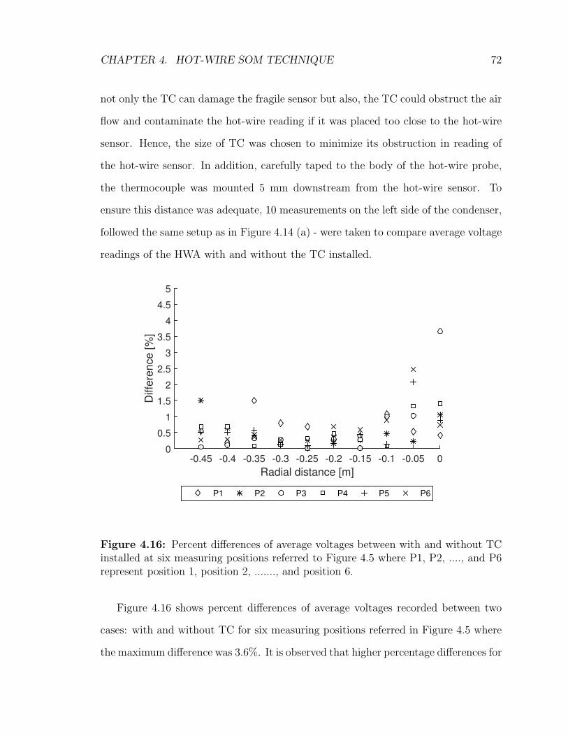
CHAPTER 4. HOT-WIRE SOM TECHNIQUE 72
not only the TC can damage the fragile sensor but also, the TC could obstruct the air
flow and contaminate the hot-wire reading if it was placed too close to the hot-wire
sensor. Hence, the size of TC was chosen to minimize its obstruction in reading of
the hot-wire sensor. In addition, carefully taped to the body of the hot-wire probe,
the thermocouple was mounted 5 mm downstream from the hot-wire sensor. To
ensure this distance was adequate, 10 measurements on the left side of the condenser,
followed the same setup as in Figure 4.14 (a) - were taken to compare average voltage
readings of the HWA with and without the TC installed.
Radial distance [m]
-0.45 -0.4 -0.35 -0.3 -0.25 -0.2 -0.15 -0.1 -0.05 0
Diffe
rence [%
]
0
0.5
1
1.5
2
2.5
3
3.5
4
4.5
5
P1 P2 P3 P4 P5 P6
Figure 4.16: Percent differences of average voltages between with and without TCinstalled at six measuring positions referred to Figure 4.5 where P1, P2, ...., and P6represent position 1, position 2, ......., and position 6.
Figure 4.16 shows percent differences of average voltages recorded between two
cases: with and without TC for six measuring positions referred in Figure 4.5 where
the maximum difference was 3.6%. It is observed that higher percentage differences for

CHAPTER 4. HOT-WIRE SOM TECHNIQUE 73
average voltages were located toward the centre rotation of the condenser fan. From
setup in Figure 4.14(a), it should be noted that the condenser fan plate was located
at a radial distance of -0.85 m to 0.85 m on the measuring line. Due to blockage
and heat effects from the motor and its plate, velocities were expected to be close to
zero while air temperatures in this region were warmer than room temperature. This
warm air contributed to the natural convection buoyancy effect on the hot-wire sensor
which increased error of hot-wire reading and resulted in higher difference between
measurements. Where air flow was intense (i.e. from -0.25 to -0.45 m on the radial
distance scale), a maximum difference was about 1.5%, which was small enough to
compromise in order to make measurements possible.
Radial distance [m]
-0.5 -0.4 -0.3 -0.2 -0.1 0 0.1 0.2 0.3 0.4 0.5
Diffe
rence [%
]
0
0.5
1
1.5
2
2.5
3
3.5
4
4.5
5
Figure 4.17: Percentage difference between temperature recorded at exact hot-wiresensor and offset locations
Moreover, temperature correction plays an important role in getting accurate
velocity calculations from the SOM. It is necessary to evaluate the temperature dif-
ference between where the hot-wire sensor is located and the offset location where the
CHAPTER 4. HOT-WIRE SOM TECHNIQUE 74
thermocouple is actually measured. Due to the accuracy limit of type-K TC (approx-
imately ± 2.2C), instead of examining half section of a measuring line, 11 locations
were measured across the condenser exit surface. Temperature percentage difference
between two setups is displayed in Figure 4.17. It is observed that the percentage
difference slightly increased toward the two edges of the measuring line. However the
maximum value (4%) was still below the error produced by type-K thermocouple for
the range of measurement in this study (17− 31C corresponding to 6 - 12 %).
4.5.3 Experimental procedure
Before any HWA measurements were taken for both cases - with and without the
VairTEX AD, AC system was run for 40 minutes to reach a steady state at 0.35
gal/min (1.32 L/min) refrigerant flow meter reading, at a low evaporator fan speed
setting. This ensured condenser fan performance as well as air temperature exiting
from the condenser discharge surface to reach a uniform state. For each study case,
the following procedure was used for 3 experimental trials for velocity measurements
collected by the HWA. Each trial was taken on a different day. It should be kept
in mind that measurement “location” was referred to a point on a measuring line.
While “position” was applied to 6 measuring orientations in the SOM.
• Probe system was locked to the furthest left measuring location - labelled 1 as
indicated in Figure 4.2.4 (a) or (b).
• Measurements were started at position 1. During this period, both hot-wire
signal and thermocouple signal were acquired simultaneously through LabVIEW
software and Omega Data Acquisition software for 30 seconds.
• The hot-wire probe was manually rotated to the next position until it reached
position 6. Measurements at each position followed the same acquiring process

CHAPTER 4. HOT-WIRE SOM TECHNIQUE 75
as position 1.
• The probe system was manually traversed to next location and the two previous
steps were repeated until data of the last location was completely achieved.
Each location took approximately 3 minutes to complete data acquisition, exclud-
ing the manual rotating time which could take up to 2 minutes.
Chapter 5
Results and Discussion
This chapter will summarize the results from the thermodynamic performance evalu-
ation on the air conditioning system described in Chapter 3. In addition, the results
from hot-wire and temperature measurements will also be discussed to characterize
air flow from condenser exit and provide a comparison of three velocity components
- radial, axial and tangential between two study cases: without and with VairTEX
AD add-on.
5.1 Air Conditioning Performance Evaluation
The AC performance was tested at 2 flow meter readings of 0.25 and 0.35 gal/min
which corresponded to refrigerant mass flow rate of 0.016 kg/s and 0.022 kg/s, cor-
respondingly, for two cases: with and without the AD. For simplification in the
discussion, all results are presented with respect to the flow meter readings instead
of refrigerant volumetric flow rate. Also, Figure 3.3 is reproduced in this section to
help the readers following the discussion easier.
76
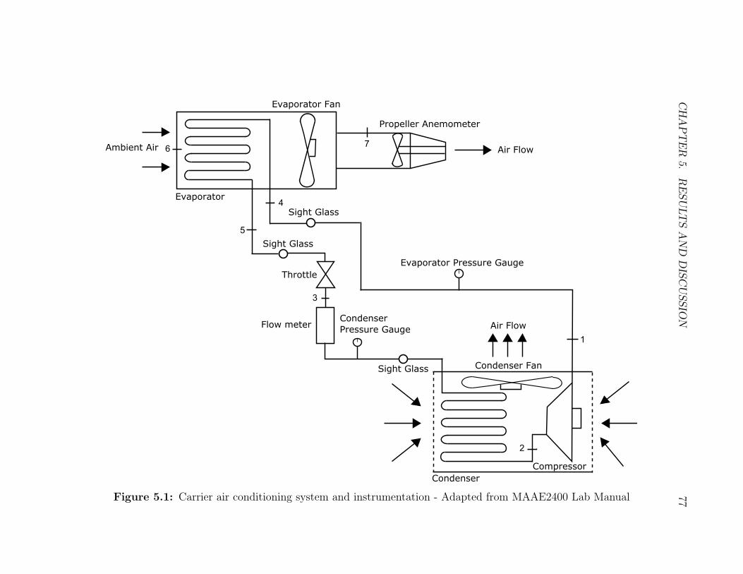
CHAPTER
5.
RESULTSAND
DISCUSSIO
N77
6
5
4
1
2
3
7
Air Flow
Condenser Fan
Compressor
Condenser
Flow meter
Sight Glass
Sight Glass
Sight Glass
Throttle
Evaporator
Evaporator Fan
Propeller Anemometer
Air FlowAmbient Air
Evaporator Pressure Gauge
Condenser
Pressure Gauge
Figure 5.1: Carrier air conditioning system and instrumentation - Adapted from MAAE2400 Lab Manual

CHAPTER 5. RESULTS AND DISCUSSION 78
5.1.1 Temperature measurements
Refrigerant temperatures
Refrigerant Flow Meter Reading [gal/min]0.25 0.35
Tem
per
atu
re[/C]
0
5
10
15
20
25
W/O VairTEX W/ VairTEX
(a) T1 - At the compressor inlet
Refrigerant Flow Meter Reading [gal/min]0.25 0.35
Tem
per
atu
re[/C]
0
10
20
30
40
50
60
70
80
90
W/O VairTEX W/ VairTEX
(b) T2 - At the condenser inlet
Refrigerant Flow Meter Reading [gal/min]0.25 0.35
Tem
per
ature
[/C]
0
5
10
15
20
25
W/O VairTEX W/ VairTEX
(c) T3 - At the throttle inlet
Refrigerant Flow Meter Reading [gal/min]0.25 0.35
Tem
per
ature
[/C]
0
5
10
15
20
25
W/O VairTEX W/ VairTEX
(d) T4 - At the evaporator exit
Refrigerant Flow Meter Reading [gal/min]0.25 0.35
Tem
per
ature
[/C]
0
2
4
6
8
10
12
W/O VairTEX W/ VairTEX
(e) T5 - At the evaporator inlet
Figure 5.2: Refrigerant temperatures recorded at five locations indicated in Figure5.1 where (a), (b), (c), (d), and (e) corresponding to location 1, 2, 3, 4, and 5 with andwithout the AD added on the condenser exit surface for two refrigerant flow meterreadings 0.25 and 0.35 gal/min

CHAPTER 5. RESULTS AND DISCUSSION 79
Refrigerant temperatures were measured at 5 locations indicated in Figure 5.1 with
and without the VairTEX AD added on. Comparisons of refrigerant temperatures
between two cases: with and without the VairTEX AD are illustrated in Figure 5.2
where (a), (b), (c), (d), and (e) correspond to temperature at measuring location 1,
2, 3, 4, and 5, respectively. It is intriguing that all refrigerant temperatures dropped
when the AD was added on the condenser. The most significant drops were 2.5C
and 2.4C for a flow meter readings of 0.25 and 0.35 gal/min respectively, which both
occurred at location 2 (after the compressor). Table 5.1 summarizes mean refrigerant
temperatures measured at five locations, as shown in Figure 5.1.
0.25 [gal/min] 0.35 [gal/min]
Variable W/O AD W AD W/O AD W AD
T1 21.3 19.6 20.5 19.3
T2 81.5 78.9 75.9 73.5
T3 21.5 20 24.0 22.2
T4 21.3 19.6 20.7 19.3
T5 3.8 2.4 10.0 9.0
Table 5.1: Refrigerant temperature (measured in C) mean values obtained fromthree repeats at two refrigerant flow rates with and without the AD
It was hypothesized that the AD increased air flow across the condenser and en-
hanced condenser coil heat rejection. Thus, the overall temperature of the refrigerant
was reduced across 5 measuring locations in the system. The answer will be revealed
in velocity measurement section.
Air temperatures
Figure 5.3 (a) and (b) displays air temperatures measured at the inlet and exit of
the evaporator while their mean values are shown in Table 5.2. As the AC system
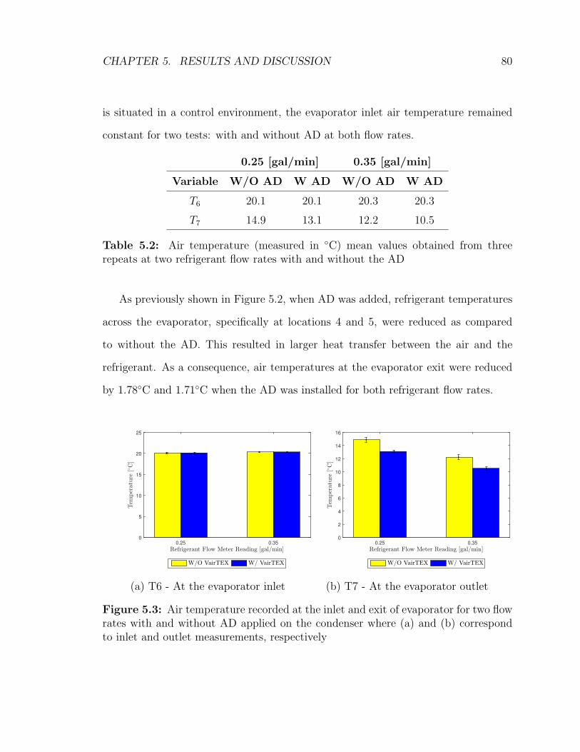
CHAPTER 5. RESULTS AND DISCUSSION 80
is situated in a control environment, the evaporator inlet air temperature remained
constant for two tests: with and without AD at both flow rates.
0.25 [gal/min] 0.35 [gal/min]
Variable W/O AD W AD W/O AD W AD
T6 20.1 20.1 20.3 20.3
T7 14.9 13.1 12.2 10.5
Table 5.2: Air temperature (measured in C) mean values obtained from threerepeats at two refrigerant flow rates with and without the AD
As previously shown in Figure 5.2, when AD was added, refrigerant temperatures
across the evaporator, specifically at locations 4 and 5, were reduced as compared
to without the AD. This resulted in larger heat transfer between the air and the
refrigerant. As a consequence, air temperatures at the evaporator exit were reduced
by 1.78C and 1.71C when the AD was installed for both refrigerant flow rates.
Refrigerant Flow Meter Reading [gal/min]0.25 0.35
Tem
per
ature
[/C]
0
5
10
15
20
25
W/O VairTEX W/ VairTEX
(a) T6 - At the evaporator inlet
Refrigerant Flow Meter Reading [gal/min]0.25 0.35
Tem
per
ature
[/C]
0
2
4
6
8
10
12
14
16
W/O VairTEX W/ VairTEX
(b) T7 - At the evaporator outlet
Figure 5.3: Air temperature recorded at the inlet and exit of evaporator for two flowrates with and without AD applied on the condenser where (a) and (b) correspondto inlet and outlet measurements, respectively
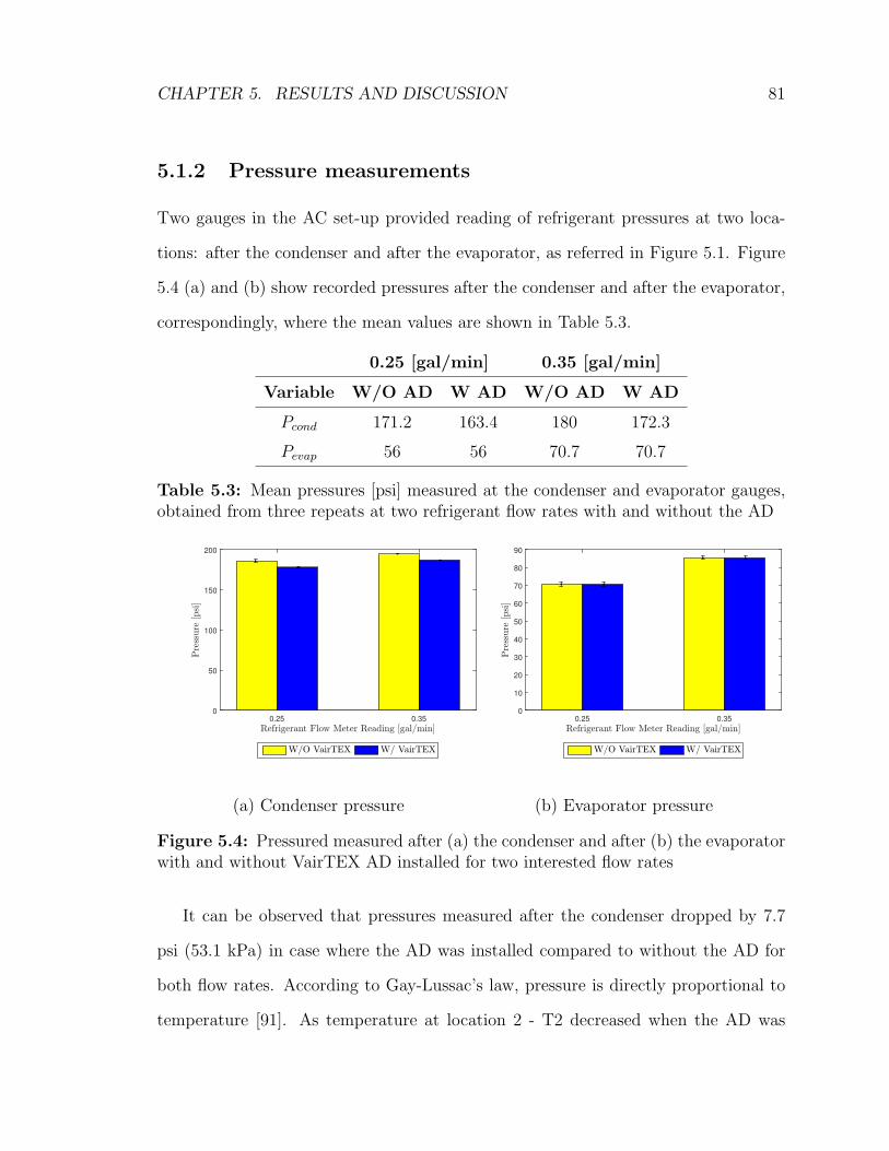
CHAPTER 5. RESULTS AND DISCUSSION 81
5.1.2 Pressure measurements
Two gauges in the AC set-up provided reading of refrigerant pressures at two loca-
tions: after the condenser and after the evaporator, as referred in Figure 5.1. Figure
5.4 (a) and (b) show recorded pressures after the condenser and after the evaporator,
correspondingly, where the mean values are shown in Table 5.3.
0.25 [gal/min] 0.35 [gal/min]
Variable W/O AD W AD W/O AD W AD
Pcond 171.2 163.4 180 172.3
Pevap 56 56 70.7 70.7
Table 5.3: Mean pressures [psi] measured at the condenser and evaporator gauges,obtained from three repeats at two refrigerant flow rates with and without the AD
Refrigerant Flow Meter Reading [gal/min]0.25 0.35
Pre
ssure
[psi]
0
50
100
150
200
W/O VairTEX W/ VairTEX
(a) Condenser pressure
Refrigerant Flow Meter Reading [gal/min]0.25 0.35
Pre
ssure
[psi]
0
10
20
30
40
50
60
70
80
90
W/O VairTEX W/ VairTEX
(b) Evaporator pressure
Figure 5.4: Pressured measured after (a) the condenser and after (b) the evaporatorwith and without VairTEX AD installed for two interested flow rates
It can be observed that pressures measured after the condenser dropped by 7.7
psi (53.1 kPa) in case where the AD was installed compared to without the AD for
both flow rates. According to Gay-Lussac’s law, pressure is directly proportional to
temperature [91]. As temperature at location 2 - T2 decreased when the AD was

CHAPTER 5. RESULTS AND DISCUSSION 82
applied, pressure recorded after the condenser was also reduced. While pressures
measured after the evaporator with and without the AD were maintained constant
for both flow rates.
5.1.3 Compressor power measurements
Figure 5.5 depicts compressor power measured when the AC system ran with and
without the AD installed on the condenser unit. An appreciable reduction in power
consumption of 3.7% and 4.5% was observed for refrigerant flow rate of 0.25 and 0.35
gal/min respectively as the AD was applied on the condenser.
Refrigerant Flow Meter Reading [gal/min]0.25 0.35
Pow
er[k
W]
0
0.5
1
1.5
W/O VairTEX W/ VairTEX
Figure 5.5: Power consumed by the compressor were recorded with and withoutVairTEX AD installed for two interested flow rates
It was found that T2 was lower in the case with the AD. As a consequent, power
consumed by the compressor was reduced. Therefore, this result showed an agreement
not only with the hypothesis made previously in which an increase in air flow across
the condenser would lower refrigerant temperature, and thus reduce compressor power

CHAPTER 5. RESULTS AND DISCUSSION 83
consumption. But also with finding from A. Elsayed as a reduction in compressor
power consumption was reported at lower condensing temperature which was achieved
by increasing air flow across the condenser [21].
As mentioned in Chapter 1, the amount of energy consumed for cooling in the
southern states of the U.S reached 129 billion kWh, during the 2009 RECS survey.
If one uses the average residential electricity rate in Texas which is 10.98 cents per
kWh. As the AD could reduce power consumption by 4.5%, it would result in saving
of 637.4 million U.S dollars, approximately. Currently, the VairTEX Canada Inc. has
not revealed the unit price of the AD applied for residential AC systems. However,
through internal discussion with the company, the unit could cost around $200 CAD.
If a 2-ton AC system consumes 2 kW per hour and runs 24/7, the electric bill could
cost $144 CAD per month for an average electric rate of 10 cents per hour. Hence,
for 4.5% power saving obtained in this study, the payback would be 3 years.
5.1.4 Refrigeration capacity
Computed based on Equation 3.8, refrigeration capacities with and without AD in-
stalled for two flow rates are presented in Figure 5.6. The thermal size of a cooling
system is known as its capacity, where it is dictated by the change in refrigerant
temperature across the evaporator coil, besides the mass flow rate of refrigerant mR22
through the coil. Higher cooling capacity is achieved by either increasing temperature
change across the coil or increase the refrigerant flow rate. As demonstrated in Figure
5.6, cooling capacity increased from 0.9 tons to 1.2 tons as refrigerant flow rate raised
from 0.25 to 0.35 gal/min, respectively. Despite lower temperature was recorded at
individual locations across the evaporator (i.e 4 and 5) in the case with the AD,
the temperature difference between location 4 and 5 remained constant regardless of
the presence of AD. This proved that the AD did not reduce or increase the cooling

CHAPTER 5. RESULTS AND DISCUSSION 84
capacity of the system.
Refrigerant Flow Meter Reading [gal/min]0.25 0.35
Ref
rige
ration
Cap
acity
[tons]
0
0.5
1
1.5
W/O VairTEX W/ VairTEX
Figure 5.6: A comparison of calculated refrigeration capacity with and without theVairTEX AD on condenser unit at different flow rates
5.1.5 Coefficient of performance (COP)
COP is determined based on Equation 3.9 as the ratio between cooling effect over
the total power input which includes power consumed by the compressor, condenser
fan and evaporator fan. First, it should be noted that no modification was made to
an inlet and outlet of the evaporator unit. Since the same working condition was
applied, mass flow across the fan remained constant in both study cases.

CHAPTER 5. RESULTS AND DISCUSSION 85
Refrigerant Flow Meter Reading [gal/min]0.25 0.35
Fre
quen
cy[H
z]
0
5
10
15
20
25
W/O VairTEX W/ VairTEX
Figure 5.7: Propeller frequency measured for two designated flow meter readingswith and without AD
Previously described in the experimental set-up of the AC system in Chapter 3,
frequency reading of the photo-chopper transducer was used to calculate air mass
flow rate across the evaporator. Figure 5.7 exhibits same frequency recorded between
two cases at two refrigerant flow meter readings. Hence, it was appropriate to assume
evaporator fan power consumption was constant between the two cases: with and
without AD.
For condenser fan, a different approach was used to verify power consumption.
The digital clamp meter Power First was used to measure the amperage drawn by
the fan. The amp reading was then utilized to evaluate the power consumption. As
shown in Figure 5.8, amperage drawn by the fan was reduced as the AD was installed
for both flow rates. However, due to the resolution of the amp clamp, the reduction
fell within the standard error of the device. Hence it is reasonable to assume the
condenser fan demands the same amount of power with and without AD presence.
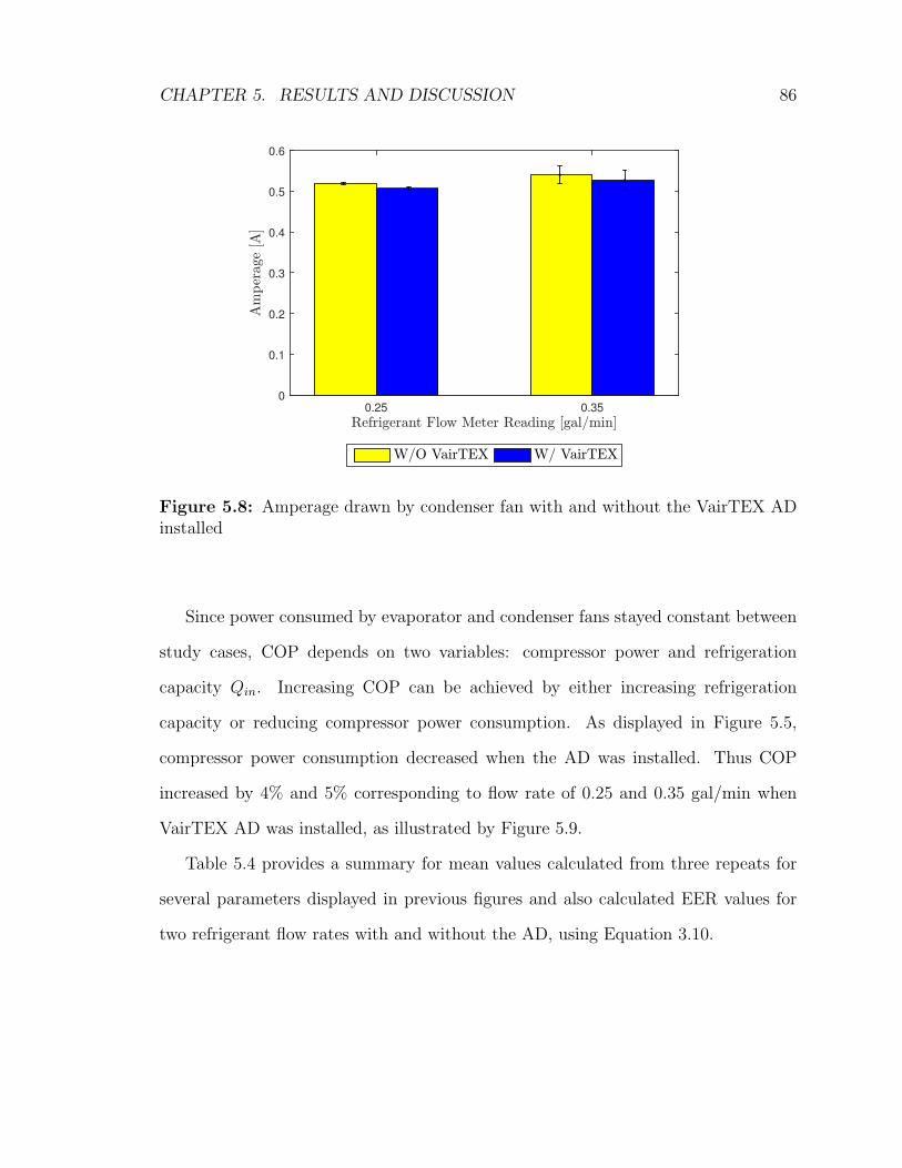
CHAPTER 5. RESULTS AND DISCUSSION 86
Refrigerant Flow Meter Reading [gal/min]0.25 0.35
Am
per
age
[A]
0
0.1
0.2
0.3
0.4
0.5
0.6
W/O VairTEX W/ VairTEX
Figure 5.8: Amperage drawn by condenser fan with and without the VairTEX ADinstalled
Since power consumed by evaporator and condenser fans stayed constant between
study cases, COP depends on two variables: compressor power and refrigeration
capacity Qin. Increasing COP can be achieved by either increasing refrigeration
capacity or reducing compressor power consumption. As displayed in Figure 5.5,
compressor power consumption decreased when the AD was installed. Thus COP
increased by 4% and 5% corresponding to flow rate of 0.25 and 0.35 gal/min when
VairTEX AD was installed, as illustrated by Figure 5.9.
Table 5.4 provides a summary for mean values calculated from three repeats for
several parameters displayed in previous figures and also calculated EER values for
two refrigerant flow rates with and without the AD, using Equation 3.10.
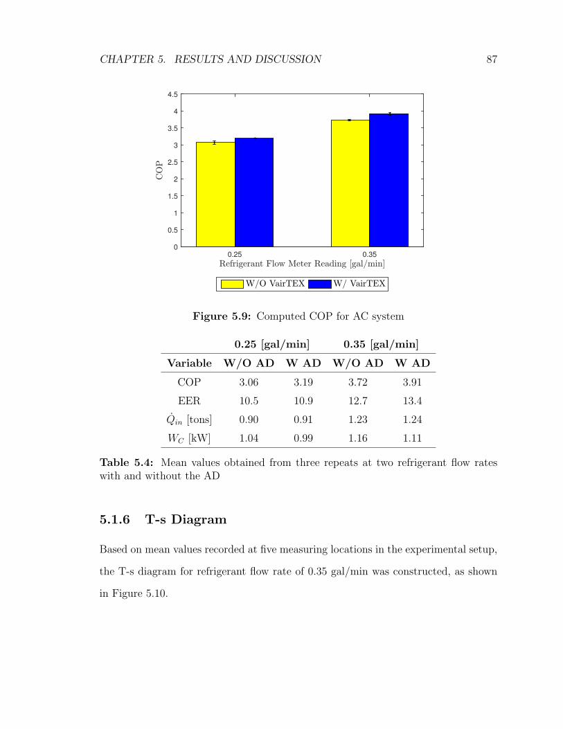
CHAPTER 5. RESULTS AND DISCUSSION 87
Refrigerant Flow Meter Reading [gal/min]0.25 0.35
CO
P
0
0.5
1
1.5
2
2.5
3
3.5
4
4.5
W/O VairTEX W/ VairTEX
Figure 5.9: Computed COP for AC system
0.25 [gal/min] 0.35 [gal/min]
Variable W/O AD W AD W/O AD W AD
COP 3.06 3.19 3.72 3.91
EER 10.5 10.9 12.7 13.4
Qin [tons] 0.90 0.91 1.23 1.24
WC [kW] 1.04 0.99 1.16 1.11
Table 5.4: Mean values obtained from three repeats at two refrigerant flow rateswith and without the AD
5.1.6 T-s Diagram
Based on mean values recorded at five measuring locations in the experimental setup,
the T-s diagram for refrigerant flow rate of 0.35 gal/min was constructed, as shown
in Figure 5.10.

CHAPTER 5. RESULTS AND DISCUSSION 88
Figure 5.10: T-s diagram comparison with and without the AD at refrigerant flowrate reading 0.35 gal/min
The blue dash line is an arbitrary line which represents the top of the liquid-
vapour dome due to the lack of data above 60C. The T-s diagram explains the
performance difference between two study cases: with and without the AD from a
thermodynamic point of view. Lower pressure during condensation process (2-3) was
recorded in case with the AD. As a consequence, the compressor work (1-2) WC was
reduced. Moreover, the throttling process in case with the AD took placed at lower
temperature, hence adding additional cooling effect to the cycle. From temperature
and enthalpy obtained after the throttle (5), calculated pressure at this location
indicated that there was a pressure drop across during the evaporation process (5-4)
for both cases. By reducing the compressor power, a slight increase in refrigeration
capacity increases COP, as the AD did in this case. Similarly, the same trend was
obtained in case at refrigerant flow rate reading of 0.25 gal/min.
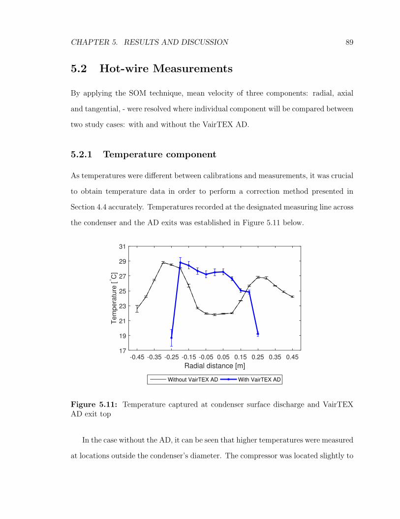
CHAPTER 5. RESULTS AND DISCUSSION 89
5.2 Hot-wire Measurements
By applying the SOM technique, mean velocity of three components: radial, axial
and tangential, - were resolved where individual component will be compared between
two study cases: with and without the VairTEX AD.
5.2.1 Temperature component
As temperatures were different between calibrations and measurements, it was crucial
to obtain temperature data in order to perform a correction method presented in
Section 4.4 accurately. Temperatures recorded at the designated measuring line across
the condenser and the AD exits was established in Figure 5.11 below.
Radial distance [m]
-0.45 -0.35 -0.25 -0.15 -0.05 0.05 0.15 0.25 0.35 0.45
Tem
pera
ture
[°C
]
17
19
21
23
25
27
29
31
Without VairTEX AD With VairTEX AD
Figure 5.11: Temperature captured at condenser surface discharge and VairTEXAD exit top
In the case without the AD, it can be seen that higher temperatures were measured
at locations outside the condenser’s diameter. The compressor was located slightly to
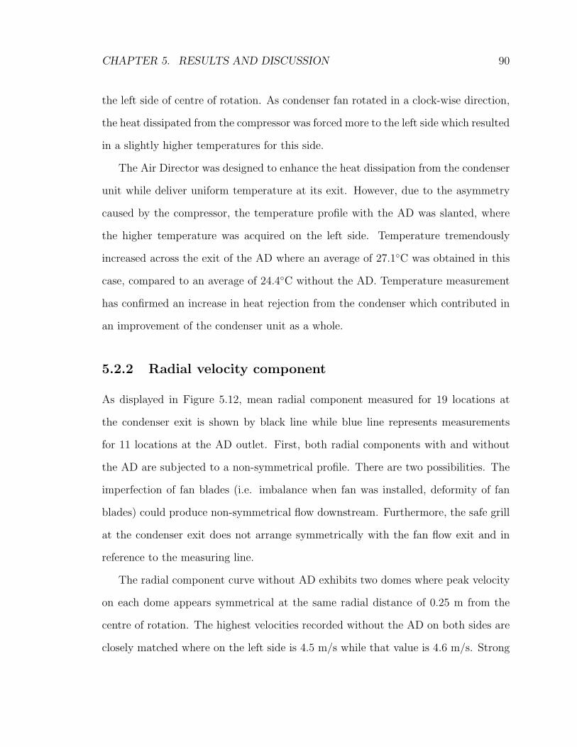
CHAPTER 5. RESULTS AND DISCUSSION 90
the left side of centre of rotation. As condenser fan rotated in a clock-wise direction,
the heat dissipated from the compressor was forced more to the left side which resulted
in a slightly higher temperatures for this side.
The Air Director was designed to enhance the heat dissipation from the condenser
unit while deliver uniform temperature at its exit. However, due to the asymmetry
caused by the compressor, the temperature profile with the AD was slanted, where
the higher temperature was acquired on the left side. Temperature tremendously
increased across the exit of the AD where an average of 27.1C was obtained in this
case, compared to an average of 24.4C without the AD. Temperature measurement
has confirmed an increase in heat rejection from the condenser which contributed in
an improvement of the condenser unit as a whole.
5.2.2 Radial velocity component
As displayed in Figure 5.12, mean radial component measured for 19 locations at
the condenser exit is shown by black line while blue line represents measurements
for 11 locations at the AD outlet. First, both radial components with and without
the AD are subjected to a non-symmetrical profile. There are two possibilities. The
imperfection of fan blades (i.e. imbalance when fan was installed, deformity of fan
blades) could produce non-symmetrical flow downstream. Furthermore, the safe grill
at the condenser exit does not arrange symmetrically with the fan flow exit and in
reference to the measuring line.
The radial component curve without AD exhibits two domes where peak velocity
on each dome appears symmetrical at the same radial distance of 0.25 m from the
centre of rotation. The highest velocities recorded without the AD on both sides are
closely matched where on the left side is 4.5 m/s while that value is 4.6 m/s. Strong

CHAPTER 5. RESULTS AND DISCUSSION 91
Radial distance [m]
-0.45 -0.35 -0.25 -0.15 -0.05 0.05 0.15 0.25 0.35 0.45
Ve
locity [
m/s
]
-0.5
0
0.5
1
1.5
2
2.5
3
3.5
4
4.5
5
Without VairTEX AD With VairTEX AD
Figure 5.12: Radial velocity component measured at condenser surface dischargeand VairTEX AD exit surface
and warm radial flow definitely affects air temperature at the intake region of the
condenser which is located around its body.
In case without AD, the region where motor’s plate exists should expect zero
velocity. However, it was shown that low velocities (maximum of 0.6 m/s) were
recorded instead. As mentioned in Chapter 4, the hot-wire sensor produces a velocity
of 0.2 m/s from its own convection effect. Additionally, the heat from the fan motor
intensifies a convection effect on the hot-wire sensor. As a consequence, velocity
readings in this region do not resolve at absolute zero.
Interestingly, when applying at the condenser exit, the AD reduces radial com-
ponent significantly. In particular, the peak velocities are reduced to a maximum of
2.2 m/s which is more than half of the peak values found in without AD case. At
locations where the motor plate exits, radial velocities emerged in this case caused
by the blade effect from the AD. Due to the blade angles of the fan and the AD,

CHAPTER 5. RESULTS AND DISCUSSION 92
their interactions could not cancel the radial components completely. Hence, the exit
flow is slightly oblique and skewed with strong flow on the left side. Moreover, as
mentioned in Chapter 1, there existed two gaps of 1.5 cm between three blade joints.
The peak appearing at the centre of the AD is induced by the air rushing through
those gaps.
5.2.3 Axial velocity component
Figure 5.13 illustrates a comparison of axial velocity component between two cases:
with and without AD installed on the condenser exit. Double-peak feature and asym-
metrical characteristics are observed for both cases. However, the AD reduces the
difference between two peak values compared to without the AD. Maximum peak val-
ues of both curves appear on the left side from the centre of rotation where highest
velocities of approximately 4 m/s were obtained in both cases. Right peak velocity
on with and without AD curves have values of 3.1 m/s and 2.7 m/s, respectively.
The most noticeable improvement of axial component appears at the centre region
where the motor plate is located. Without AD, the plate causes stagnation in this
region where maximum velocity is only 0.6 m/s. The same reason discussed in radial
profile section is applied in this low flow region. However, when the AD is installed
the axial flow is significantly increased at the centre. As exit flow from the fan was
forced to escape through the cylindrical body of the AD, a sufficient height between
the condenser exit and the AD blades allow the flow to develop at the centre.
In addition, by applying the trapezoid rule for two outlets: condenser and AD
where the radial distance is kept constant from -0.25 to 0.25 m for comparison purpose,
the volumetric flow rate Q can be approximated based on the axial velocity profile.
A pronounced increment in volumetric flow rate of 48.7% was recorded when AD was

CHAPTER 5. RESULTS AND DISCUSSION 93
Radial distance [m]
-0.45 -0.35 -0.25 -0.15 -0.05 0.05 0.15 0.25 0.35 0.45
Ve
locity [
m/s
]
-0.5
0
0.5
1
1.5
2
2.5
3
3.5
4
4.5
5
Without VairTEX AD With VairTEX AD
Figure 5.13: Axial velocity contour collected at condenser surface discharge andVairTEX AD exit surface
installed. Hence, the hypothesis discussed in section 5.1.1 is proven here. An increase
in axial flow also enhances heat rejection by the condenser. Consequently, condensing
temperature drops, thus compressor power consumption is reduced.
5.2.4 Tangential velocity component
As exit flow in both study cases is three dimensional, tangential component, also
called swirling component, should be examined as well. Figure 5.14 displays tangential
velocity component obtained from two study cases: with and without the VairTEX
AD.
In the case without the AD, tangential flow pattern follows a similar trend to
radial and axial profiles as shown in Figure 5.12 and 5.13 above. No actual flow was
recorded at stagnation region due to the presence of a motor plate. Values obtained
in this region were caused solely by the convection effect from the hot-wire sensor.
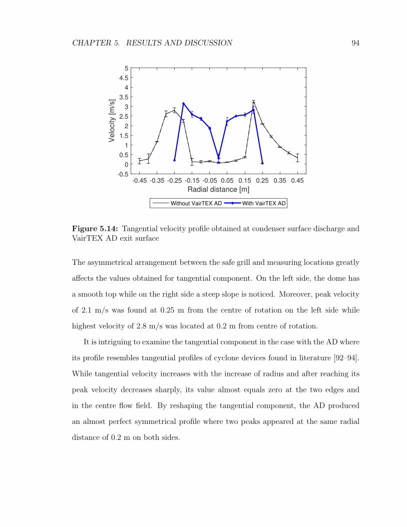
CHAPTER 5. RESULTS AND DISCUSSION 94
Radial distance [m]
-0.45 -0.35 -0.25 -0.15 -0.05 0.05 0.15 0.25 0.35 0.45
Ve
locity [
m/s
]
-0.5
0
0.5
1
1.5
2
2.5
3
3.5
4
4.5
5
Without VairTEX AD With VairTEX AD
Figure 5.14: Tangential velocity profile obtained at condenser surface discharge andVairTEX AD exit surface
The asymmetrical arrangement between the safe grill and measuring locations greatly
affects the values obtained for tangential component. On the left side, the dome has
a smooth top while on the right side a steep slope is noticed. Moreover, peak velocity
of 2.1 m/s was found at 0.25 m from the centre of rotation on the left side while
highest velocity of 2.8 m/s was located at 0.2 m from centre of rotation.
It is intriguing to examine the tangential component in the case with the AD where
its profile resembles tangential profiles of cyclone devices found in literature [92–94].
While tangential velocity increases with the increase of radius and after reaching its
peak velocity decreases sharply, its value almost equals zero at the two edges and
in the centre flow field. By reshaping the tangential component, the AD produced
an almost perfect symmetrical profile where two peaks appeared at the same radial
distance of 0.2 m on both sides.
CHAPTER 5. RESULTS AND DISCUSSION 95
5.3 Uncertainty Analysis
No measurement can be performed with perfect certainty. Errors always exit in
any experimental measurement where it exists in two forms: systematic errors and
random errors. Systematic errors are defined as errors that affect the accuracy of a
measurement. On the other hand, random errors are caused by the precision of a
measurement. In this study, the systematic errors will be evaluated, following rules
detailed in Appendix A.
5.3.1 Velocity measurement
Calibration setup error
The core of the calibration system used for hot-wire is the flow meter which has
an accuracy of ± 0.7% on output reading, according to the manufacture calibration
certificate. The nozzle was 3D printed where the design diameter was 18 mm. To
quantify the uncertainty on the nozzle outlet diameter, three measurements were
taken using Mastercraft digital caliper with accuracy of ± 0.02 mm. The average
diameter of nozzle from three measurements is 17.84 mm. By taking into account
the error from caliper measurement, the nozzle diameter reading can be expressed as
17.84 mm ± 0.2% which results in an uncertainty of ± 0.28% for nozzle area. The
uncertainty of velocity calculated using Equation 4.34 is considered to be ± 0.75%.
Temperature correction error
Errors in temperature correction are evaluated for both calibration and measurement.
The lowest temperature recorded in calibration was 20C while this value in measure-
ment was 17.4C. Following Equation 4.44, when correction is performed, velocity is
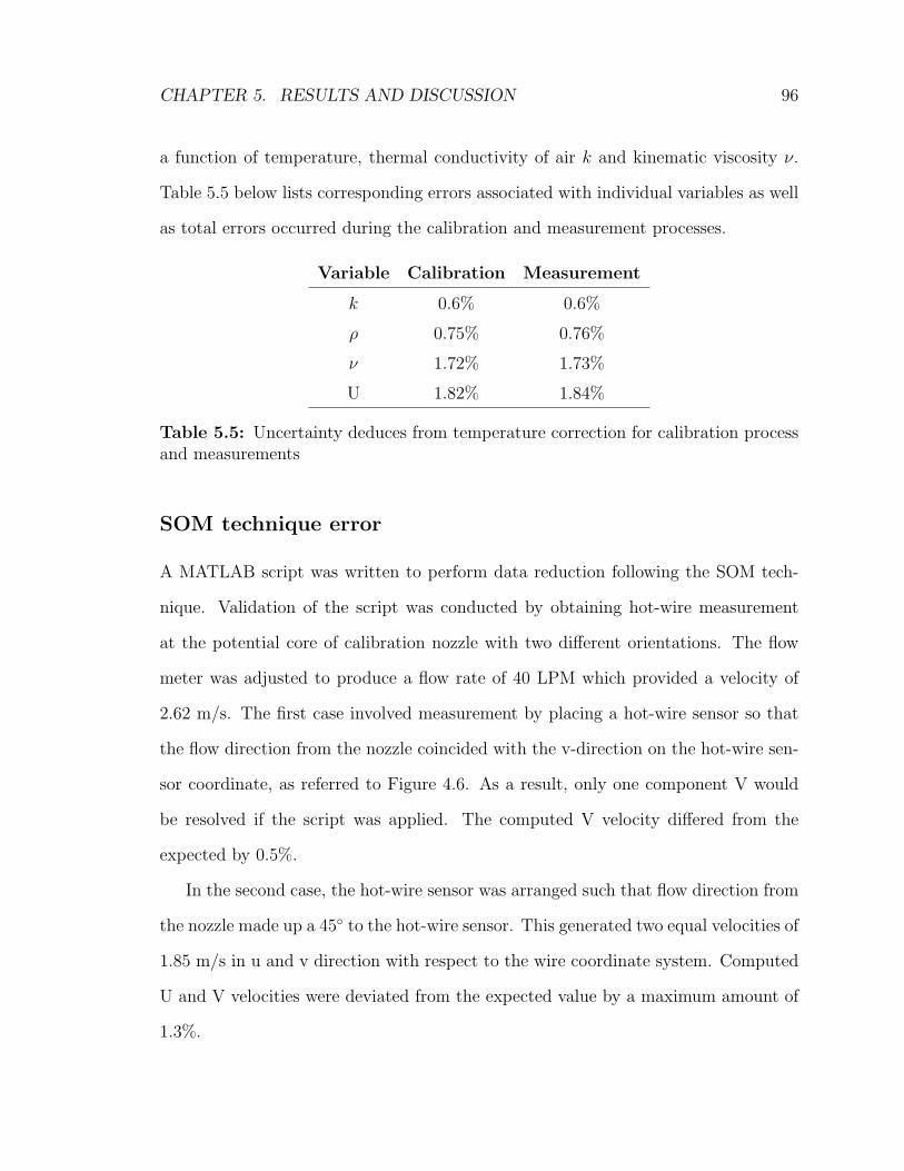
CHAPTER 5. RESULTS AND DISCUSSION 96
a function of temperature, thermal conductivity of air k and kinematic viscosity ν.
Table 5.5 below lists corresponding errors associated with individual variables as well
as total errors occurred during the calibration and measurement processes.
Variable Calibration Measurement
k 0.6% 0.6%
ρ 0.75% 0.76%
ν 1.72% 1.73%
U 1.82% 1.84%
Table 5.5: Uncertainty deduces from temperature correction for calibration processand measurements
SOM technique error
A MATLAB script was written to perform data reduction following the SOM tech-
nique. Validation of the script was conducted by obtaining hot-wire measurement
at the potential core of calibration nozzle with two different orientations. The flow
meter was adjusted to produce a flow rate of 40 LPM which provided a velocity of
2.62 m/s. The first case involved measurement by placing a hot-wire sensor so that
the flow direction from the nozzle coincided with the v-direction on the hot-wire sen-
sor coordinate, as referred to Figure 4.6. As a result, only one component V would
be resolved if the script was applied. The computed V velocity differed from the
expected by 0.5%.
In the second case, the hot-wire sensor was arranged such that flow direction from
the nozzle made up a 45 to the hot-wire sensor. This generated two equal velocities of
1.85 m/s in u and v direction with respect to the wire coordinate system. Computed
U and V velocities were deviated from the expected value by a maximum amount of
1.3%.
CHAPTER 5. RESULTS AND DISCUSSION 97
Moreover, mean velocity of three components: radial, axial, and tangential were
established using SOM technique derived by King [49]. The uncertainty associated
with this method was reported by Janjua in mean velocities measurement of a confined
jet with a value of 5% [95]. Hence, the uncertainty using the SOM technique in this
work is assumed to be 5%.
Six-axis rotation device
The CNC machine used to manufacture the six-axis rotation device has an accuracy
of about ± 0.0254 mm (0.001′′), therefore can be considered dimensionally accurate.
Two levels were installed on the six-axis rotation device in order to align probe co-
ordinate to the condenser’s. Both indicators of two levels have accuracy of ± 0.1.
If misalignment occurred in the worse case scenario, one of the components would
be off by a value of cos 0.1 × cos 0.1 which is insignificant for minimum considered
velocity value of 0.4 m/s (lowest value obtained after exclude values from convection
effect). Hence this error can be neglected.
Geometric scale of traverse system
Marking at every 5 cm interval on the traverse beam was made using a metric ruler
with graduation of 0.1 cm. Thus, the precision can be considered to be± 0.05 cm. The
largest uncertainty from geometric markings occurred in the case of velocity measure-
ment without VairTEX AD at 19 locations which produced a combined uncertainty
of ± 0.22 cm. The probe system can be positioned by the user at each location with
an accuracy of ± 0.1 cm approximately. The total error in the positioning process of
19 locations produces uncertainty of ± 0.44 cm. Therefore, the combined uncertainty
is estimated to be ± 0.49 cm or ± 0.54% for total measurement length of 90 cm.
CHAPTER 5. RESULTS AND DISCUSSION 98
Taking into account all discussed errors, the total uncertainty accumulated from
velocity measurement is approximate 5.9% at 95% confidence level.
5.3.2 AC Performace Evaluation
Refrigeration capacity
Refrigeration capacity Qin is calculated based on mass flow rate of refrigerant and
two enthalpies where their values are estimated based on pressure and temperature
collected at locations 4 and 3 (assuming h3 = h5).
The accuracy provide by the flow meter manufacture is 4% full scale of 0.7 GPM
which corresponds to uncertainty of ± 11.2% at lowest flow rate reading of 0.25 GPM.
Since υR22 varies insignificantly over a change in temperature of ± 2.2C (maximum
0.73% change in value), the accuracy of mR22 solely depends on accuracy of flow
meter. Hence, mR22 has an uncertainty of ± 11.2%.
TC type J has an accuracy of ± 2.2C while pressure gauges have accuracy of 2%,
based on manufacture technical specification. By varying temperatures and pressures
within their accuracies, change in values of enthalpies h4 and h5. It was observed that
temperature had a higher influence to value of h4 in compare to pressure. However,
the change in value of h4 due to temperature change is insignificant as the highest per-
centage change was 0.6% which can be neglected. Enthalpy is assumed to be constant
across the throttle, therefore, accuracy of h5 depends on the temperature measured
at location 3, as refrigerant is in saturated liquid state before the throttle. The error
of h5 is 3.9% obtained by varying temperature at measuring location 3. Therefore,
the error for enthalpy difference can be approximated using error in calculation of h5.
Combining two uncertainties in refrigeration capacity calculation, the total error
CHAPTER 5. RESULTS AND DISCUSSION 99
is about 11.8% for measurement at 0.25 gal/min. Applying this procedure, the un-
certainty of Qin measured at 0.35 gal/min is approximately 8.9%. It can be seen in
this study, the accuracy of the flow meter has contributed greatly to the accuracy of
Qin calculation.
COP
Since COP is calculated based on computed refrigeration capacity and measured
power from the compressor. The Wavetek DM7 has accuracy of ± 0.8% while the
refrigeration capacity has uncertainty of 11.8% and 8.9% for flow rate reading of 0.25
gal/min and 0.35 gal/min correspondingly. Therefore the uncertainty associated with
COP for two refrigerant flow rates are 11.8% and 8.9% approximately.
5.3.3 Random error
AC performance
The main purpose of this study was to compare the performance of an AC system with
and without the VairTEX Air Director. Since same AC system was used throughout
the whole study, both cases and systematic errors are ‘one-sided’ error. Therefore, it
is more interesting to look into the statistical significance of data obtained.
Generally, p-value is used as a tool to evaluate a statistical significance. The P
value is defined as the probability under the assumption of no effect or no difference
(null hypothesis), of obtaining a result equal to or more extreme than what was
actually observed. The P stands for ‘Probability’ and measures how likely it is that
any observed difference between groups is due to chance [96]. To find p-value between
two sets of data, a ‘Student-t-test’ is employed. Typically, in most engineering works,
a difference is said to be statistically significance if p-value is less than 0.05. Hence,

CHAPTER 5. RESULTS AND DISCUSSION 100
in this work, critical p-value of 0.05 will be used.
P-values in this study are assessed based on data from three trials performed for
each case of interest: with and without the VairTEX AD. The most important factors
to evaluate an AC system performance include: COP, refrigeration capacity (Qin),
power consumption (specifically in this study power consumed by the compressor),
and air temperature produced after passing through the evaporator (T6). Table
5.6 shows several p-values obtained from comparison data of interest variables listed
above between with and without using the AD at two flow meter reading 0.25 and
0.35 gal/min. A p-value of less than 0.05 indicates that there is a significant difference
between two cases: with and without AD applied on the condenser. In particular,
there exists an improvement by using the AD. It can be seen that p-values of COP,
compressor power, and T6 for both flow meter reading are all less than 0.05. Hence,
it is demonstrated that they are statistically significant differences.
Flow meter reading [gal/min]
Variable 0.25 0.35
COP 0.008 0.001
Qin 0.29 0.03
Wc 0.0025 0.0008
T6 0.0009 0.0065
Table 5.6: Summary p-values for several interested variables collected from ACperformance evaluation
Velocity and temperature measurements
Three velocity components: radial, axial, and tangential along with temperature mea-
surement at each measuring location were averaged from three trials. Since hot-wire
has minimum velocity sensitivity of 0.2 m/s, therefore uncertainties for three veloc-
ity components with values less than 0.2 m/s will not be computed due to error
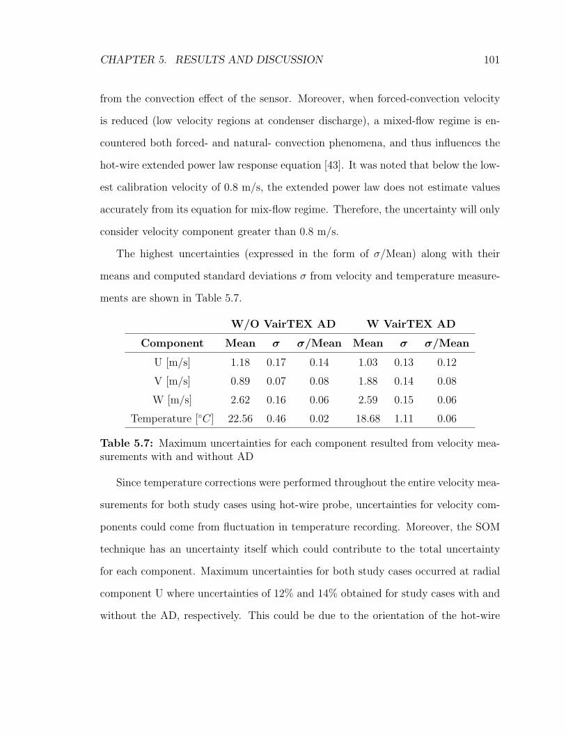
CHAPTER 5. RESULTS AND DISCUSSION 101
from the convection effect of the sensor. Moreover, when forced-convection velocity
is reduced (low velocity regions at condenser discharge), a mixed-flow regime is en-
countered both forced- and natural- convection phenomena, and thus influences the
hot-wire extended power law response equation [43]. It was noted that below the low-
est calibration velocity of 0.8 m/s, the extended power law does not estimate values
accurately from its equation for mix-flow regime. Therefore, the uncertainty will only
consider velocity component greater than 0.8 m/s.
The highest uncertainties (expressed in the form of σ/Mean) along with their
means and computed standard deviations σ from velocity and temperature measure-
ments are shown in Table 5.7.
W/O VairTEX AD W VairTEX AD
Component Mean σ σ/Mean Mean σ σ/Mean
U [m/s] 1.18 0.17 0.14 1.03 0.13 0.12
V [m/s] 0.89 0.07 0.08 1.88 0.14 0.08
W [m/s] 2.62 0.16 0.06 2.59 0.15 0.06
Temperature [C] 22.56 0.46 0.02 18.68 1.11 0.06
Table 5.7: Maximum uncertainties for each component resulted from velocity mea-surements with and without AD
Since temperature corrections were performed throughout the entire velocity mea-
surements for both study cases using hot-wire probe, uncertainties for velocity com-
ponents could come from fluctuation in temperature recording. Moreover, the SOM
technique has an uncertainty itself which could contribute to the total uncertainty
for each component. Maximum uncertainties for both study cases occurred at radial
component U where uncertainties of 12% and 14% obtained for study cases with and
without the AD, respectively. This could be due to the orientation of the hot-wire

CHAPTER 5. RESULTS AND DISCUSSION 102
probe with radial velocity direction. In other words, the prong effect from the hot-
wire probe caused greater aerodynamic disturbance in radial component than other
velocity components.
For temperature measurements, maximum uncertainty of 6% came from the mea-
suring point located just outside of discharged surface of the AD. Refer to Figure 4.14
(b) measurements at two edges basically represent room temperatures. As the lab
room temperature dropped suddenly during a recording of one data set, the mean
temperature resulted to this high standard deviation. Other than this, if measurement
is considered just within the plumes, the highest uncertainty is about 2.25%.
Chapter 6
Conclusions and Recommendations for
Future Work
6.1 AC Performance Evaluation
Conclusion from AC performance evaluation will be summarized in the section below.
Also, recommendations for future work in this particular study will be discussed.
6.1.1 Conclusion
Despite the maturity of the AC system, there is still room available for improvement.
VairTEX has demonstrated its advantage in enhancing performance AC system, in
particular reducing power consumption by the compressor while allowing the evap-
orator unit deliver cooler air at its exit. The following section summarizes findings
throughout the performance evaluation of the AC system. P-values were computed
to ensure differences were statistically significant.
• COP was improved by an appreciable of 4% at refrigerant flow meter reading
of 0.25 gal/min while at 0.35 gal/min COP was enhanced by 5%, with respect
to mean values for both flow rates. Caution is advised from using these values
103
CHAPTER 6. CONCLUSIONS AND RECOMMENDATIONS 104
because of the uncertainty level for COP calculation.
• Compressor power demand reduced by 3.7% and 4.5% with respect to mean
values for refrigerant flow meter readings of 0.25 and 0.35 gal/min, respectively.
• AC system operated with VairTEX produced same refrigeration capacity as
when it ran without the device.
6.1.2 Recommendations
• Improvement was demonstrated on a 20 year-old AC system. Majority AC
systems using in Canada however have a maturity age of approximately 10
years, as discussed in Chapter 2. To convince more residential customers, testing
should be performed on a more modern unit, as well as units from broader AC
manufacturers. In addition, CSA test standards CSA C656-05 and CAN/CSA-
C656-14 should also be consulted for performance evaluation.
• In order to provide a more in-depth evaluation on the effectiveness of the AD,
the condenser unit should be installed in a controlled environment - separately
from the evaporator unit - where temperatures surrounding the condenser can
be adjusted to represent a ‘real-world’ situation, for example summer seasonal
temperatures. In addition, cross-wind has proven to effect dispersion of plumes
discharged at an air-cooled condenser [9]. Hence, an artificial cross-wind can
be introduced at the condenser unit to further assess the effectiveness of the
VairTEX AD.
• Pressures on the refrigerant line were measured at two locations: after the
condenser and after the evaporator. It was assumed that pressure remained
constant across the condenser and evaporator. This does not reflect pressure

CHAPTER 6. CONCLUSIONS AND RECOMMENDATIONS 105
loss which does occur along the refrigerant line. More gauges could be installed
to obtain more accurate thermodynamic data at selected measuring locations on
refrigerant line, for example: before and after the compressor, after the throttle,
and before the evaporator coil.
• Besides an already existing power meter for a compressor, an additional power
meter could be installed for the whole AC system to eliminate an assumption
on evaporator fan power consumption.
• Also, the AC system could be installed in a higher ceiling room to minimize the
effect of the ceiling on the plume discharge, especially in the case with the AD
installed on top of the condenser unit.
6.2 Velocity and Temperature Measurements
Velocity measurements at condenser exit and AD exit were performed by applying
the six-orientation measurement technique on a single hot-wire. Temperature mea-
surements were also conducted not only to correct hot-wire data but also to explain
such improvements in thermodynamic performance at the condenser unit. Similar
to previous section, a conclusion and future work for velocity measurement will be
detailed below.
6.2.1 Conclusion
• The AD completely modified profiles of each individual velocity component. Es-
pecially at the stagnation region where the motor plate was located, additional
flow was introduced at this region.

CHAPTER 6. CONCLUSIONS AND RECOMMENDATIONS 106
• The dominant velocity in case without the AD was a radial component while it
was found to be an axial component with the presence of the AD.
• With the presence of the AD, the radial profile was reduced significantly and
redistributed to the axial component which resulted in an increase of volumetric
flow rate by a substantial amount of 48.7%. This demonstrated that exit flow
was not only straightened by the AD but also increased volume flow rate through
its top surface.
• By straightening the exit flow, the AD isolated exit plumes from the intake flow
of the condenser unit which then allowed cooler air to enter the condenser unit.
• Additionally, cyclonic behaviour was also observed in the case with the AD,
as its tangential velocity profile was similar to one found in studies of cyclone
devices.
• Temperature profile measured at the AD top exit demonstrated an increase in
heat dissipation from the condenser unit. As a result, refrigerant temperature
was reduced - hence, reducing compressor work.
6.2.2 Recommendations
• To have a more accurate velocity measurement in three-dimensional turbulent
flow field, cross-wire or triple-wire hot-wire probe should be used. In addition,
flow visualization methods such as PIV can provide precise details at circulation
zone where HWA is incapable of providing similar information.
• A thermal camera such as infrared camera could be use to provide a graphic
illustration on dissipation of heat from the condenser with and without the AD.

CHAPTER 6. CONCLUSIONS AND RECOMMENDATIONS 107
• Besides, a parametric study on different body sizes (diameter, height) and
shapes (diffuser, nozzle, straight cylinder with and without blades), blade angles
and dimensions is interesting to investigate in order to optimize performance of
the AD, and thus maximize improvement on the AC system.
• Lastly, a numerical work could also be used to perform parametric study on
blade shape and angle, as well as body augmentation of the AD.

List of References
[1] US Department of Energy, “History of Air Conditioning.” https://energy.
gov/articles/history-air-conditioning/, 2017. Accessed: 10/10/2017.
[2] US Department of Energy, “Heating and cooling no longer majority of U.S home
energy use.” https://www.eia.gov/todayinenergy/detail.php?id=10271&
src=%E2%80%B9%20Consumption%20%20%20%20%20%20Residential%20Energy%
20Consumption%20Survey%20(RECS)-f1#, 2013. Accessed: 10/10/2017.
[3] howstuffworks, “How to Repair Central Air Conditioner.” http:
//home.howstuffworks.com/home-improvement/heating-and-cooling/
how-to-repair-central-air-conditioners.htm, 2017. Accessed:
10/10/2017.
[4] Goverment of Canada, “2011 survey of household energy use (sheu),” tech.
rep., Natural Resources Canada, 2015. http://www.nrcan.gc.ca/energy/
efficiency/17097.
[5] Goverment of Canada, “Energy efficiency trends in canada 1990 to 2013,” tech.
rep., Natural Resources Canada, 2016.
[6] Natural Resources Canada, “Central Air CConditioner.” http://www.
nrcan.gc.ca/energy/products/categories/cooling-ventilating/
air-conditioning/central/16183, 2017. Accessed: 11/10/2017.
[7] “2008 standard for performance rating of unitary air-conditioning & air-source
heat pump equipment.”
[8] VairTEX Canada Inc., “Vairtex technical description,” tech. rep., VairTEX
Canada Inc., 2017.
[9] K. Khankari, “Optimum placement for air-cooled chillers,” ASHRAE, vol. 58,
2016.
108
109
[10] G. A. Godbout and D. A. C. Godbout, “Air conditioner turbulence creating
energy saver,” Jan. 2015.
[11] VairTEX Canada Inc., “Internal communication report.” October 2017.
[12] E. G. Pita, Air Conditioning Principles and Systems - An Energy Approach.
John Wiley & Sons, 1989.
[13] V. V. Birangane and A. M. Patil, “Comparison of air cooled and evaporatively
cooled refrigeration systems - a review paper,” International Journal of Engi-
neering Research and Applications, vol. 4, pp. 208–211, June 2014.
[14] T. C. Kandpal, “Improved efficiency ccompressor for air conditioning,” in Inter-
national Compressor Engineering Conference, School of Mechanical Engineering
- Purdue University, 1978.
[15] A. Sakuda, K. Sawai, N. Lida, A. Hiwata, and T. Morimoto, “Performance
improvement of scroll compressor with new sealing-oil supply mechanism,” in
Compressors and Their Systems: 7th International Conference, 2001.
[16] J. K. Sonne, D. S. Parker, and S. F. Barhaszi, eds., Measured Impacts of Air
Conditioner Condenser Shading, Florida Solar Energy Center, American Council
for an Energy-Efficient Economy, 2002.
[17] A. I. ElSherbini and G. P. Maheshwari, eds., Effectiveness of Shading Air-cooled
Condensers of Air-conditioning systems, (Kuwait), Proceedings of the Tenth
International Conference for Enhanced Building Operations, Oct 2010.
[18] G. H. Donovan and D. T. Butry, “The value of shade: Estimating the effect of
urban trees on summertime electricity use,” Energy and Buildings, vol. 41, no. 6,
pp. 662–668, 2009.
[19] M. A. Hoeschele, M. J. Berman, L. E. Elberling, and M. B. Hunt, eds., Evapo-
rative Condensers: The Next Generation in Residential Air Conditioning, Davis
Energy Group and Pacific Gas & Electric Company, American Council for an
Energy-Efficient Economy, 1998.
[20] D. S. Parker, J. R. Sherwin, and R. A. Raustad, “Improving best air conditioner
efficiency by 20-30stage coupled with an evaporative condenser pre-cooler,” tech.
rep., Florida Solar Energy Center, 2014.

110
[21] A. O. Elsayed and A. S. Hariri, eds., Effect of condenser air flow on the Perfor-
mance of split air conditioner, World Renewable Energy Congress, (Linkoping,
Sweden), University of Dammam, Saudi Arabia, Low-Energy Architecture, May
2011.
[22] P. N. Ananthanarayanan, Basic Refrigeration and Air Conditioning. Tata
McGraw-Hill, 2005.
[23] Gemaire Distributors, “Fan blades.” https://gemaire.com/. Accessed:
10/17/2017.
[24] R. C. Monroe, “Improving cooling tower fan system efficiencies,” in Seventh
Turbomachinery Symposium, vol. 50, Hudson Products Corporation, May 1978.
[25] D. S. Parker, J. R. Sherwin, and B. Hibbs, “Development of high efficiency air
conditioner condenser fans,” ASHRAE Transactions, 2005. Florida.
[26] N. C. Kernstock, “Slashing through the noise barrier,” Aviation Today, August
1999.
[27] T. Iwase, E. Katayama, S. Sekiya, and T. Kishitani, “Development of high ef-
ficiency fan system for outdoor unit of air-conditioner,” JRAIA International
Symposium, 2016.
[28] ebmpapst, “The axitop diffuser,” tech. rep., ebmpapst Group, 2017.
[29] O. Igra, “Research and development for shrouded wind turbines,” Energy Con-
version and Management, vol. 21, no. 1, pp. 13–48, 1981.
[30] Y. Ohya and T. Karasudani, “A shrouded wind turbine generating high output
power with wind-lens technology,” Energies, vol. 3, pp. 634–649, 2010.
[31] Y. Ohya, T. Karasudani, T. Nagai, and K. Watanabe, “Wind lens technology
and its application to wind and water turbine and beyond,” Renewable Energy
and Environmental Sustainability, vol. 2, no. 2, 2017.
[32] P. B. Kosasih, N. Bryce, A. Tondelli, and A. Beazley, “Experimental study of
the performance of bare and nozzle - diffuser shrouded micro wind turbine un-
der axial and non-axial inflow condition,” in 18th Australasian Fluid Mechanics
Conference, School of Mechanial, Materials and Mechatronics Engineering, Uni-
versity of Wollongong, New South Wales, Australia, 2012.
111
[33] G. Balaji and I. Gnanambal, “Wind power generator using horizontal axis wind
turbine with convergent nozzle,” Journal of Scientific & Industrial Research,
vol. 73, pp. 375–380, 2014.
[34] N. A. Pambudi, D. L. Pristiandaru, Basori, D. S. Wijayanto, H. Bugis, B. D.
Wahyudi, C. Sudibyo, K. M.W., N. Rahman, N. Sriwardani, and Subagsono,
“Experimental investigation of wind turbine using nozzle-lens at low wind speed
condition,” in Energy Procedia, vol. 105, pp. 1063–1069, 2017. 8th International
Conference on Applied Energy ICAE2016.
[35] D. C. Look Jr. and H. J. Sauer Jr., Engineering Thermodynamics. PWS Engi-
neering, 1986.
[36] American Chemical Society, “Chlorofluorocarbons and Ozone Depletion.”
http://www.acs.org/content/acs/en/education/whatischemistry/
landmarks/cfcs-ozone.html, 2017. Accessed: 2/10/2017.
[37] M. J. Moran, H. N. Shapiro, D. D. Boettner, and M. B. Bailey, Fundamentals of
Engineering Thermodynamics. Wiley and Sons, eight ed., 2014.
[38] Mechanical and A. Engineering, MAAE 2400 Thermodynamics and Heat Trans-
fer Laboratory Instructions. Carleton University.
[39] Wavetek, “Wavetek dm7 handheld digital multimeter manual,” tech. rep.
[40] A. Inc., “2071a contractor pressure gauge,” tech. rep., 2017.
[41] C. G. Lomas, Fundamentals of Hot Wire Anemometry. Cambridge University
Press, 1986.
[42] G. Comte-Bellot, “Hot-wire anemometry,” Fluid Mechanics, vol. 8, pp. 209–231,
1976.
[43] H. H. Bruun, Hot-Wire Anemometry Principles And Signal Analysis. Oxford
University Press, 1985.
[44] E. Rathakrishman, Theoretical Aerodynamics. Wiley and Sons, 2013.
[45] F. E. Jorgensen, “How to measure turbulence with hot-wire anemometers,” tech.
rep., Dantec Dynamics, 2002.

112
[46] A.A. Lab Systems Ltd., “How to adjust the frequency response of a CT anemome-
ter.” http://www.lab-systems.com/products/flow-mea/Adjusting%20the%
20frequency%20response/Adjusting%20the%20frequency%20response.
html, 2017. Accessed: 4/10/2017.
[47] L. V. King, “On the convection of heat from small cylinders in a stream of
fluid: Determination of the convection constants of small platinum wires with
applications to hot-wire anemometry,” Philosophical Transactions of the Royal
Society of London, May 1914.
[48] H. H. Bruun, M. A. Khan, H. H. Al-Kayiem, and A. A. Fardad, “Velocity cali-
bration relationships for hot-wire anemometry,” Journal of Physics E: Scientific
Instruments, vol. 21, no. 2, p. 225, 1988.
[49] C. F. King, Some Studies of Vortex Devices - Vortex Amplifier Performance
Behavior. PhD thesis, University College of Wales, Cardiff, Wales, 1978.
[50] F. E. Jorgensen, “Directional sensitivity of wire and fiber-film probes,” DISA
Information, May 1971.
[51] N. Syred, J. M. Beer, and N. A. Chigier, “Turbulence measurements in swirling
recirculating flows,” in Proceedings: Salford Symposium on Internal Flows,
pp. B27–B36, London, England: Institute of Mechanical Engineering, 1971.
[52] I. Wygnanski and H. Fielder, “Some measurements in the self preserving jet,”
Journal of Fluid Mechanics, vol. 38, p. 577, 1969.
[53] B. D. Pratte and J. R. Keffer, “The swirling turbulent jet,” Journal of Basic
Engineering, vol. 94, pp. 739–748, 1972.
[54] K. Dvorak and N. Syred, “The statistical analysis of hot-wire anemometry signals
in complex flow fields,” in Proceeding DISA Conference, University of Leicester,
vol. 1, pp. 136–144, Leicester University Press, 1972.
[55] C. F. King, “Vortex amplifier internal geometry and its effect on performance,”
International Journal of Heat and Mass Transfer, vol. 6, pp. 160–170, September
1985.
[56] S. I. Janjua, “Turbulence measurements in a complex flowfield using a six-
orientation hot-wire probe technique,” Master’s thesis, Oklahoma State Uni-
versity, 1981.
113
[57] A. A. Sveshnikov, Problems in Probability Theory - Mathematical Statistics and
Theory of Random Functions. W.B. Saunders Company, 1968.
[58] J. O. Hinze, Turbulence. McGraw Hill, 2nd ed., 1975.
[59] S. McTavish, Identification of wind turbine testing practices and investigation
of the performance benefits of closely-spaced lateral wind farm configurations.
phdthesis, Carleton University, 2013.
[60] X. Grandchamp, A. V. Hirtum, and X. Pelorson, “Hot-film/hot-wire calibra-
tion for low to moderate flow velocities,” Measurement Science and Technology,
vol. 21, May 2010.
[61] X. Grandchamp, Y. Fujiso, B. Wu, and A. Van Hirtum, “Steady laminar axisym-
metrical nozzle flow at moderate reynolds numbers: Modmodel and experiment,”
Journal of Fluids Engineering, vol. 134, 2012.
[62] M. Gad-el-Hak, Frontiers in Experimental Fluid Mechanics. Springer Berlin
Heidelberg, 1989.
[63] L. Cattafesta, C. J. Bahr, and J. Mathew, “Fundamentals of wind-tunnel design,”
Experimental Techniques for Fluid Dynamics and Thermal Science, 2010.
[64] R. D. Mehta, “The aerodynamic design of blower tunnels with wide-angle dif-
fusers,” Progress in Aerospace Sciences, vol. 18, pp. 59–120, 1979.
[65] W. H. Rae Jr. and A. Pope, Low-Speed Wind Tunnel Testing. John Wiley &
Sons, 1984.
[66] V. Chandavari and S. Palekar, “Diffuser angle control to avoid flow separation,”
International Journal of Technical Research and Applications, vol. 2, pp. 16–21,
Sep-Oct 2014.
[67] P. W. Runstadler Jr., “Diffuser data book,” Tech. Rep. Note 186, Creare Inc.
Tech., Hanover, NH, 1975.
[68] F. M. White, Fluid Mechanics. McGraw Hill, fifth ed., 2003.
[69] J. H. Bell and R. D. Mehta, “Design and calibration of the mixing layer and wind
tunnel,” tech. rep., Department of Aeronautics and Astronautics - Standford
University and NASA, 1989.

114
[70] G. G. Borger, “The optimization of wind tunnel ccontraction for the subsonic
range,” tech. rep., NASA, 1976.
[71] T. Morel, “Comprehensive design of axisymmetric wind tunnel contractions,”
Journal of Fluid Engineering, 1975.
[72] Y. Su, “Flow analysis & design of three-dimensional wind tunnel contractions,”
AIAA Journal, vol. 29, no. 11, 1992.
[73] A. E. Perry, Hot-wire Anemometry. Oxford Science Publications, 1982.
[74] D. C. Collis and M. J. Williams, “Two-dimensional convection from heating wires
at low reynolds numbers,” Journal of Fluid Mechanics, vol. 6, pp. 357–84, 1959.
[75] H. P. Grant and R. E. Kronauer, “Fundamentals of hot-wire anemometry,” Symp.
on Measurements in Unsteady Flow, pp. 44–53, 1962. Worcester,MA: American
Society of Mechanical Engineers.
[76] P. W. Bearman, “Corrections for the effect of ambient temperature drift on hot-
wire measurements in incompressible flow,” DISA Information, no. 11, pp. 25–30,
1971.
[77] A. Abdel-Rahman, C. Tropea, P. Slawson, and A. Strong, “On temperature
compensation in hot-wire anemometry,” Journal of Physics E: Scientific Instru-
ments, no. 20, pp. 315–9, 1987.
[78] S. F. Benjamin and C. A. Roberts, “Measuring flow velocity at elevated temper-
ature with a hot-wire anemometer calibarted in cold flow,” International Journal
of Heat and Mass Transfer, no. 45, pp. 703–706, 2002.
[79] C. Tropea, A. L. Yarin, and J. F. Foss, Springer Handbook of Experimental Fluid
Mechanics. Springer Berlin Heidelberg, 2007.
[80] M. Hultmark and A. J. Smits, “Temperature corrections for constant temper-
ature and constant current hot-wire anemometers,” Measurement Science and
Technology, 2010.
[81] D. Dynamics, Single sensor miniature wire Probes. Dantec Dynamics, 2017.
[82] A. Van Dijk and F. T. M. Nieuwstadt, “The calibration of multi-hot-wire probe:
1. temperature calibration,” Experiments in Fluids, vol. 36, pp. 540–9, 2004.

115
[83] W. G. Kannuluik and E. H. Carman, “The temperature dependence of the
thermal conductivity of air,” Australian Journal of Scientific Research, vol. 4,
pp. 305–14, 1951.
[84] J. C. Dixon, The shock absorber handbook. John Wiley & Sons Ltd, second ed.,
2007.
[85] A.A. Lab Systems Ltd., AN-1005 Hot-wire & hot-film anemometry Systems:
User’s Manual.
[86] S. C. Morris, J. J Good, and J. F. Foss, “Velocity measurements in the wake of
an automotive cooling fan,” Experimenteal Thermal and Fluid Science, vol. 17,
pp. 100–106, 1998.
[87] N. L. Gifford, A. G. Hunt, E. Savory, and R. J. Martinuzzi, “Experimental study
of low-pressure automotive cooling fan aerodynamics under blocked conditions,”
CSME Forum, 2006.
[88] M. B. Sekularac, “Experimental determination of tunnel ventilation axial ducted
fan performance,” Thermal Science, vol. 20, no. 1, pp. 209–221, 2016.
[89] X. Zhao, J. Sun, and Z. Zhang, “Prediction and measurement of axial flow
fan aerodynamic and aeroacoustic performance in a split-type air-conditioner
outdoor unit,” International Journal of Refrigeration, vol. 36, pp. 1098–1108,
2013.
[90] C. Xu and R. S. Amano, “Unsteady pressure fiield investigation of an axial fan
- blade unsteady pressure field measurement,” International Journal of Rotating
Machinery, vol. 8, no. 6, pp. 385–395, 2002.
[91] K. M. Tenny and J. S. Cooper, “Chemistry, ideal gas behavior.” https://www.
ncbi.nlm.nih.gov/books/NBK441936/, Oct 6 2017. Accessed: 10/30/2017.
[92] F. Kaya, I. Karagoz, and A. Avci, “Effects of surface roughness on the perfor-
mance of tangential inlet cyclone separators,” Aerosol Science and Technology,
vol. 45, pp. 988–995, 2011.
[93] J. Cernecky and K. Plandorova, “The effect of the introduction of an exit tube
on the separation efficiency in a cyclone,” Brazilian of Chemical Engineering,
vol. 30, pp. 627–641, July-September 2013.

116
[94] L. Liu, H. S. Dou, X. P. Chen, and H. Z. Zhang, “Analysis of vortex flow in
a cyclone separators based on the energy gradient theory,” in IOP Conference
Series: Materials Science and Engineering, no. 72, 2015.
[95] S. I. Janjua, D. K. Mclaughlin, D. G. Lilley, and T. Jackson, “Turbulence mea-
surements in a confined jet using a six-orientation hot-wireprobel technique,”
techreport, NASA, 1982.
[96] S. N. Goodman, “P value hypothesis and likelihood: implications for epidemiol-
ogy of a neglected historical debate,” American Journal Epidemiology, vol. 137,
pp. 485–96, 1993.
[97] Michigan State University, “Error propagation.” http://lectureonline.cl.
msu.edu/~mmp/labs/error/e2.htm,Aug.2016. Accessed: 11/13/2017.
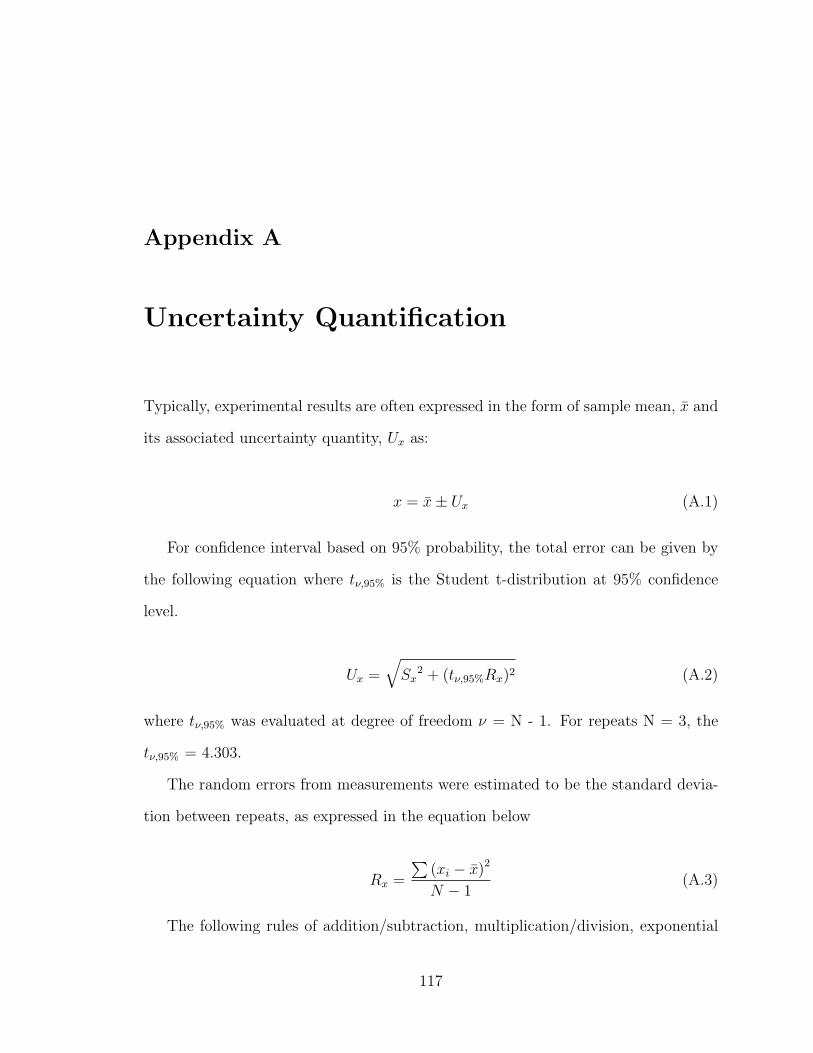
Appendix A
Uncertainty Quantification
Typically, experimental results are often expressed in the form of sample mean, x and
its associated uncertainty quantity, Ux as:
x = x± Ux (A.1)
For confidence interval based on 95% probability, the total error can be given by
the following equation where tν,95% is the Student t-distribution at 95% confidence
level.
Ux =√
Sx2 + (tν,95%Rx)2 (A.2)
where tν,95% was evaluated at degree of freedom ν = N - 1. For repeats N = 3, the
tν,95% = 4.303.
The random errors from measurements were estimated to be the standard devia-
tion between repeats, as expressed in the equation below
Rx =
∑
(xi − x)2
N − 1(A.3)
The following rules of addition/subtraction, multiplication/division, exponential
117
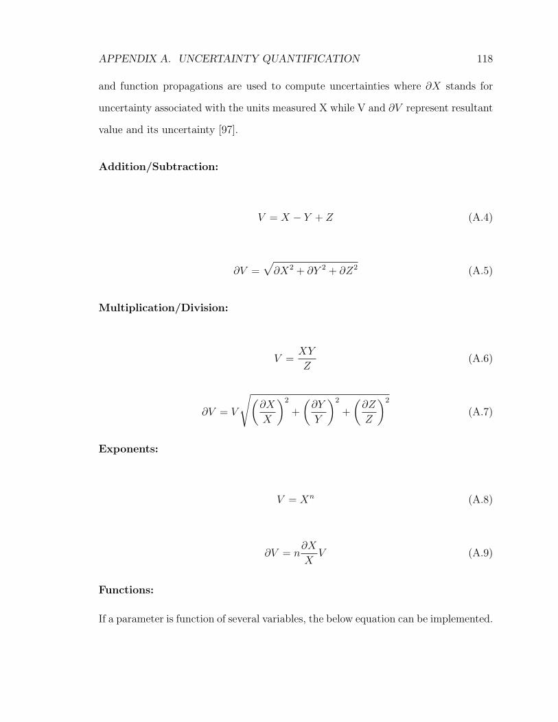
APPENDIX A. UNCERTAINTY QUANTIFICATION 118
and function propagations are used to compute uncertainties where ∂X stands for
uncertainty associated with the units measured X while V and ∂V represent resultant
value and its uncertainty [97].
Addition/Subtraction:
V = X − Y + Z (A.4)
∂V =√
∂X2 + ∂Y 2 + ∂Z2 (A.5)
Multiplication/Division:
V =XY
Z(A.6)
∂V = V
√
(
∂X
X
)2
+
(
∂Y
Y
)2
+
(
∂Z
Z
)2
(A.7)
Exponents:
V = Xn (A.8)
∂V = n∂X
XV (A.9)
Functions:
If a parameter is function of several variables, the below equation can be implemented.
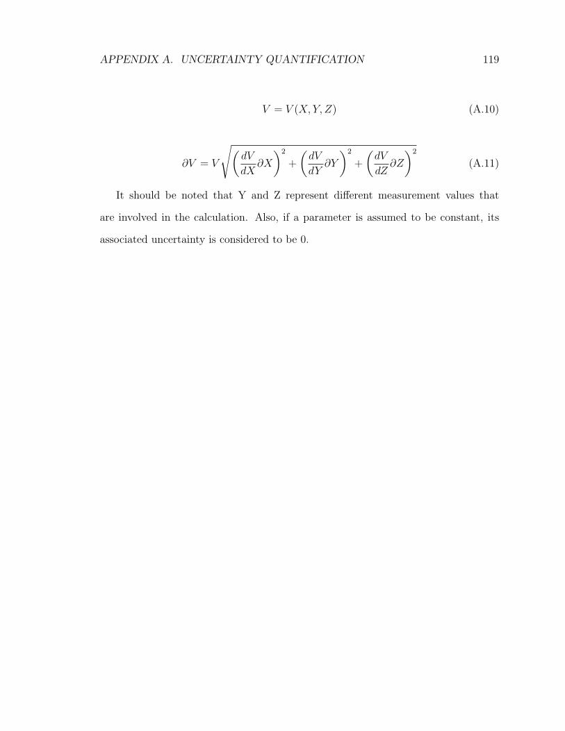
APPENDIX A. UNCERTAINTY QUANTIFICATION 119
V = V (X, Y, Z) (A.10)
∂V = V
√
(
dV
dX∂X
)2
+
(
dV
dY∂Y
)2
+
(
dV
dZ∂Z
)2
(A.11)
It should be noted that Y and Z represent different measurement values that
are involved in the calculation. Also, if a parameter is assumed to be constant, its
associated uncertainty is considered to be 0.