11TH INTERNATIONAL SYMPOSIUM ON PARTICLE IMAGE VELOCIMETRY – PIV15

Santa Barbara, California, September 14-16, 2015

PIV Uncertainty: Computational & Experimental

Evaluation of Uncertainty Methods

Aaron Boomsma1, Sayantan Bhattacharya

2, Dan Troolin

1, Pavlos Vlachos

2, & Stamatios Pothos

1

1 Fluid Mechanics Research Instruments, TSI Incorporated, Shoreview, MN, USA

aaron.boomsma@tsi.com

2 School of Mechanical Engineering, Purdue University, West Lafayatte, Indiana, USA

ABSTRACT

Uncertainty quantification for planar PIV remains a challenging task. In the present study, we assess three methods that

were recently described in the literature: primary peak ratio (PPR), mutual information (MI), and image matching (IM).

Each method was used to calculate the uncertainty in a synthetic turbulent boundary layer flow and an experimental jet

flow. In the experimental case, two PIV systems with common fields of view were used—one with a high dynamic range

(which was considered as the true solution) and another with a magnification ratio of about four times less (which was

considered the measurand). The high resolution PIV system was verified by comparing velocity records at a point with an

LDV measurement system. PIV processing was performed with PRANA and Insight4G. In regards to the experimental

flow, the PPR method performed best, followed by mutual information, and lastly image matching. This was due to better

responses by PPR and MI of uncertainty to the spatially varying error distribution. Similar conclusions were made with

respect to the synthetic test case.

1. Introduction and Background Information

Every experimental measurement method has errors associated with it, usually categorized either as a random or bias error

(Coleman & Steele, 2009). It is, therefore, critical that the measurement device have some uncertainty reported along with

each measurement. A measurement’s uncertainty is defined as a bound in which, at some level of confidence, it is believed

that the measurement error resides. Particle Image Velocimetry (PIV) is an established fluid mechanics measurement

methodology whose uncertainty has been undergoing renewed study since 2012.

Although the sources of PIV measurement error are well known (Huang et al., 1997, Raffel, 2013), quantifying their

corresponding uncertainty bounds continues to be a challenge. This is, in part, due to the high number of sources of error,

nonetheless their interactions. PIV measurement errors can be caused by hardware/experimental setup (calibration error,

background noise, out-of-plane particle motion, particle response, peak locking, non-uniform particle reflection etc.) and

algorithm selection (interrogation window size, strong velocity gradients within windows, peak detection scheme, etc.).

Each of these sources of error can manifest itself as a random or bias error.

Recently, there have been a number of excellent studies that have investigated uncertainty quantification in PIV

measurements, including Timmins et al. 2012, Sciacchitano et al. (2013), Weineke (2015), Charonko & Vlachos (2013),

Xue et al. (2014), and Xue et al. (2015). Each of which has developed algorithms to predict 2D PIV measurement

uncertainty. Many of these algorithms were compared to one another under various flow conditions, as was reported in

Sciacchitano et al. (2014). In that publication, it was shown that each uncertainty method had its own strengths and

weaknesses, and under various conditions, no one method was able to perfectly compute PIV measurement uncertainty.

Furthermore, new methods of uncertainty prediction have since come forth. Therefore, to further elucidate 2D PIV

measurement uncertainty, it is our goal to compare and contrast select uncertainty prediction methods in real and synthetic

flows.

2. Processing & Uncertainty Quantification Methods

Current literature puts forth, in general, three approaches to quantifying uncertainty in 2D PIV measurements, seemingly

each with its own advantages and disadvantages. These approaches can be categorized as follows: 1) uncertainty surface

methods; 2) image matching methods; and 3) correlation plane methods. We give a brief description of each approach

herein, along with a description of the PIV processing schemes and codes used in the present work.

2.1 Uncertainty Surface Methods

Uncertainty surface methods (see Timmins et al., 2010, Timmins et al., 2012) utilize a priori knowledge about an error

source and its corresponding measurement error (i.e., the response to some error source) to predict uncertainty. This type of

uncertainty method is, at a foundational level, similar to the works of Kahler et al. (2012) and Fincham & Delerce (2000).

Using this approach, one selects some number of error sources and creates synthetic images from a defined velocity field

while methodically varying the error source. Then, after processing the images, errors can be defined for each velocity

vector. In this way, one can isolate error and the error source, and in turn, create an uncertainty surface of responses for the

selected error sources. Timmins et al. (2012) have investigated particle image size, seeding density, shear rate, and particle

displacement as potential error sources. The uncertainty surface method is performed like a post-processing method and

requires some software-specific calibration.

2.2 Image Matching Methods

Image matching methods (Sciacchitano et al., 2013) calculate PIV measurement uncertainties by matching individual

particle images from a given interrogation window at time t to the same window at time t+Δt, where Δt signifies the time

between the laser pulse. Particle matching is achieved by shifting the window by a local processed displacement vector. For

particles that are matched, any spatial difference between them is recorded as a disparity vector. An ensemble of disparity

vectors is collected and after statistical analysis, a value of uncertainty can be calculated. Similar to the particle disparity

method of Sciacchitano et al. (2013) is the method of Weineke (2015), termed correlation statistics. The primary difference

between the two is that correlation statistics method utilizes all particle images within an interrogation window, not just

those that were matched. The correlation statistics method calculates PIV uncertainty by adding displacements to a

correlation map until its correlation peak is symmetrical. Image matching methods occur after vector processing and require

a converged velocity vector field.

2.3 Correlation Plane Methods

Correlation plane methods have been in development since the work of Charonko et al. (2013). These types of uncertainty

methods solely utilize the correlation plane. In Charonko et al. (2013), the authors found that the magnitude of the

displacement error is inversely proportional to the Primary Peak Ratio (PPR), or the ratio between primary and secondary

correlation peaks. The authors argued that the PPR is the natural choice for uncertainty analysis because the Signal-to-

Noise Ratio (SNR) encompasses all possible sources of error. As such, the authors formulated a relation between the PPR

and the error, with software-specific fitting coefficients calculated from synthetic data. A year later, Xue et al. (2014)

furthered this work by relating not only the PPR and error, but also other measures of the SNR, such as peak-to-root mean

square ratio, peak-to-correlation energy, and cross-correlation entropy. Xue et al. (2014) also formulated a new relation

between the SNR and displacement error that does not assume a normal distribution of measurement error.

Xue et al. (2015) also proposed uncertainty quantification using a new metric, MI or Mutual Information. The MI is the

ratio of the cross-correlation peak to the auto-correlation peak of an ideal Gaussian particle and denotes the effective

amount of correlating information. It is a measure of NIFIFO. A higher MI suggests a higher number of particles correlating

within the interrogation windows and thus the true displacement can be measured with a lesser uncertainty. Xue et al.

(2015) calculated a calibration to predict the PIV measurement uncertainty as a function of MI and the authors

demonstrated excellent uncertainty coverage for each test case.

2.4 PIV Processing Algorithms

In the present study, our collaboration has enabled us to study uncertainty methods as implemented in different PIV

processing codes. The codes utilized in this paper were: an in-house open source code (PRANA, Vlachos 2015), and

Insight4G (TSI Inc.) Each was used to measure the low and high resolution PIV data sets, and therefore throughout this

study, we present results from each. Processing in each code occurred as follows:

PRANA: Low resolution data sets were processed using the Standard Cross-Correlation (SCC) with multi-pass

iterative window deformation method. A window resolution of 64x64pix was used for the first two

iterations and 32x32 for next three iterations, with a final pass grid overlap of 75%.

High resolution data sets were processed using the Robust Phase Correlation (RPC) method (Eckstein et

al., 2008; Eckstein & Vlachos, 2009). Six passes of window deformation were performed with a final

pass window resolution of 48x48 and 84% grid overlap.

Validation, UOD median filtering and smoothing were done in between passes to achieve a converged

velocity field. The final pass results without validation are used for uncertainty analysis.

Insight4G: Low resolution data sets were processed using the SCC method. Window deformation was utilized;

five primary iterative passes with 80x80pix interrogation windows occurred along with three secondary

passes at 32x32pix windows. Between passes, vector outlier detection and replacements, along with

low-pass filtering occurred, but on the last pass, no such filling or filtering was utilized. High resolution

data sets were processed using the same conditions as the low resolution parameters.

Three uncertainty models are assessed in this paper, and they include:

1. PPR uncertainty method of Xue et al. (2014) as implemented in both PRANA and Insight4G.

2. Mutual information uncertainty method of Xue et al. (2015), implemented in PRANA.

3. Particle disparity method of Sciacchitano et al. (2013), implemented in PRANA.

3. Description of Test Cases

In order to assess the performance of each method, it is paramount that the measurement error be well known. For the

synthetic flow, the error is known due to the prescribed displacement (i.e., the true solution) of the particle images, but in an

experimental flow, the true solution is unknown. We therefore follow the approach of Sciacchitano et al. (2015) and utilize

two synchronized sets of PIV systems: a low resolution (measurement) and high resolution (reference) PIV system. To

validate that the high resolution PIV system approximates the true solution, we compare its results with Laser Doppler

Velocimetry (LDV) measurements.

3.1 Synthetic Test Case

The reference flow for the computational evaluation of uncertainty methods is a fully-developed turbulent boundary layer

flow that was obtained from the Johns Hopkins Turbulence Database (Li et al., 2008). The boundary layer was simulated

with Direct Numerical Simulation (DNS) with approximately 1.6 billion nodes. The shear velocity Reynolds number,

and is defined as:

where √ is the shear velocity, is the half-channel height of the computational domain, and is the kinematic

viscosity. The Navier-Stokes equations were integrated in time using a third-order Runge-Kutta method with periodic

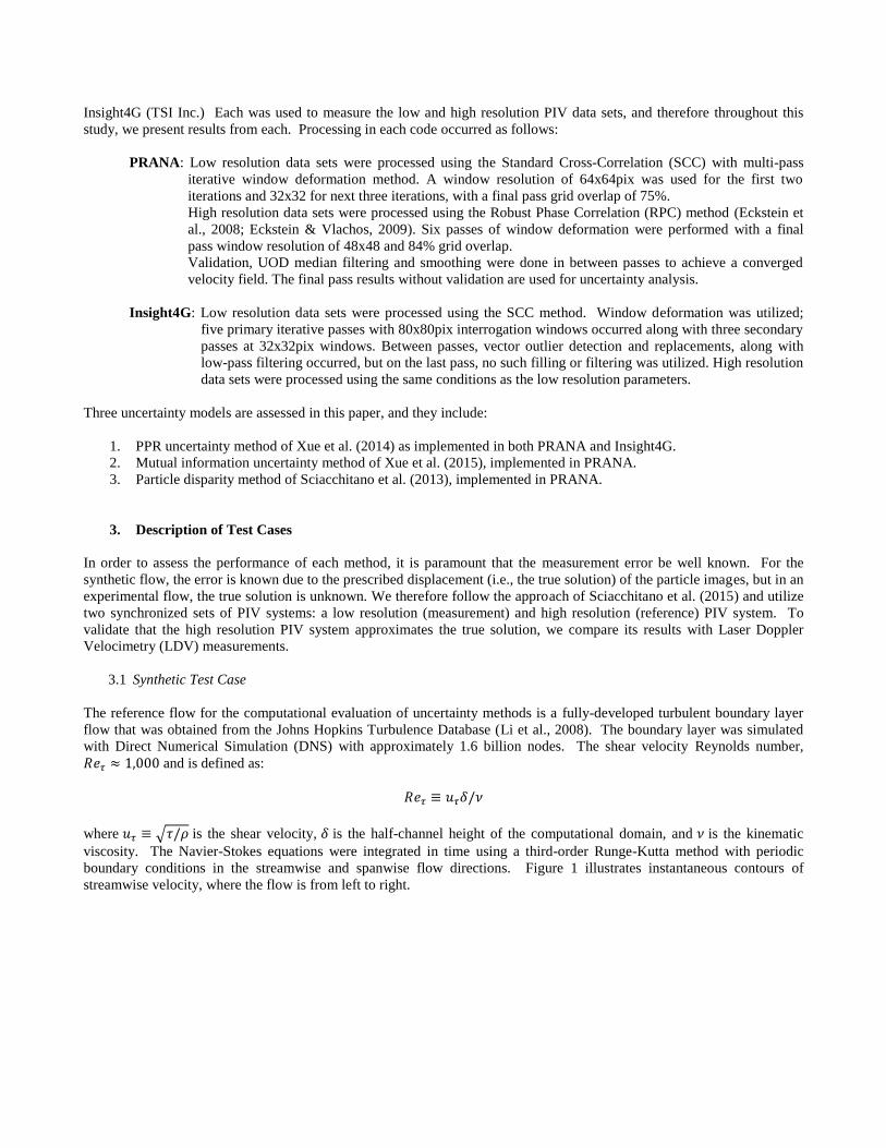
boundary conditions in the streamwise and spanwise flow directions. Figure 1 illustrates instantaneous contours of

streamwise velocity, where the flow is from left to right.

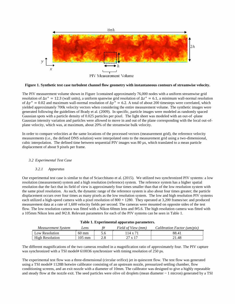
Figure 1. Synthetic test case turbulent channel flow geometry with instantaneous contours of streamwise velocity.

The PIV measurement volume shown in Figure 1contained approximately 76,000 nodes with a uniform streamwise grid

resolution of (wall units), a uniform spanwise grid resolution of , a minimum wall-normal resolution

of and maximum wall-normal resolution of . A total of about 200 timesteps were correlated, which

yielded approximately 700k velocity vectors when considering the entire measurement volume. The synthetic images were

generated following the guidelines of Brady et al. (2009). In specific, particle images were modeled as randomly spaced

Gaussian spots with a particle density of 0.025 particles per pixel. The light sheet was modeled with an out-of -plane

Gaussian intensity variation and particles were allowed to move in and out of the plane corresponding with the local out-of-

plane velocity, which was, at maximum, about 20% of the streamwise bulk velocity.

In order to compare velocities at the same locations of the processed vectors (measurement grid), the reference velocity

measurements (i.e., the defined DNS solution) were interpolated onto to the measurement grid using a two-dimensional,

cubic interpolation. The defined time between sequential PIV images was 80 µs, which translated to a mean particle

displacement of about 9 pixels per frame.

3.2 Experimental Test Case

3.2.1 Apparatus

Our experimental test case is similar to that of Sciacchitano et al. (2015). We utilized two synchronized PIV systems: a low

resolution (measurement) system and a high resolution (reference) system. The reference system has a higher spatial

resolution due the fact that its field of view is approximately four times smaller than that of the low resolution system with

the same pixel resolution. As such, the dynamic range of the reference system is also about four times greater; the particle

displacement occurs over four times as many pixels as the low resolution system. The low and high resolution PIV systems

each utilized a high-speed camera with a pixel resolution of 800 × 1280. They operated at 3,200 frames/sec and produced

measurement data at a rate of 1,600 velocity fields per second. The cameras were mounted on opposite sides of the test

flow. The low resolution camera was fitted with a Nikon 60mm lens and f#5.6. The high resolution camera was fitted with

a 105mm Nikon lens and f#2.8. Relevant parameters for each of the PIV systems can be seen in Table 1.

Table 1. Experimental apparatus parameters.

Measurement System Lens f# Field of View (mm) Calibration Factor (um/pix)

Low Resolution 60 mm 5.6 114 x 71 88.41

High Resolution 105 mm 2.8 27 x 17 21.48

The different magnifications of the two cameras resulted in a magnification ratio of approximately four. The PIV capture

was synchronized with a TSI model# 610036 synchronizer with timing resolution of 250 ps.

The experimental test flow was a three-dimensional (circular orifice) jet in quiescent flow. The test flow was generated

using a TSI model# 1128B hotwire calibrator consisting of an upstream nozzle, pressurized settling chamber, flow

conditioning screens, and an exit nozzle with a diameter of 10mm. The calibrator was designed to give a highly repeatable

and steady flow at the nozzle exit. The seed particles were olive oil droplets (mean diameter ~ 1 micron) generated by a TSI

model# 9302 atomizer and introduced into the settling chamber. The flow immediately downstream of the nozzle exit was

steady and laminar. A schematic of the velocity measurement systems can be seen in Figure 2. The PIV laser shown in

Figure 2 was a dual-head Nd:YLF laser with each head operating at 1,600 pulses/sec with a light sheet thickness of

approximately 1.2mm.

Figure 2. Experimental arrangement of the velocity measurement systems. The dashed lines downstream of the jet

orifice denote the different fields of view for the low and high resolution PIV systems.

In order to verify the accuracy of the high resolution (reference) PIV system, we compared processed vectors from it with

synchronized measurements from an LDV reference system. The LDV was considered as the ground truth and consisted of

a TSI solid state Powersight LDV. The LDV measurement volume was aligned to measure the streamwise velocity

component of the jet and the intersecting laser beams were in the plane of the PIV laser sheet. A 250mm focal distance lens

was used, and the LDV measurement volume size was an ellipsoid with dimensions of 88 microns in the PIV streamwise

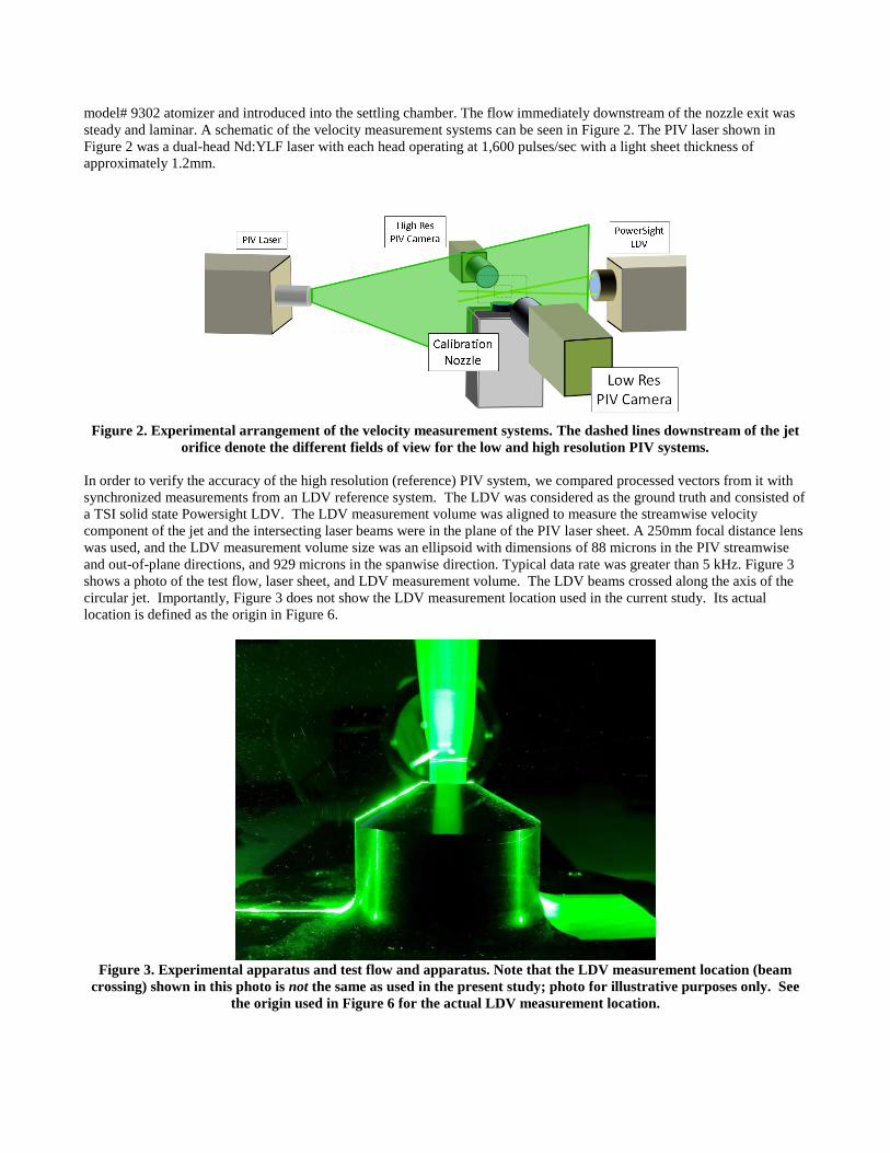
and out-of-plane directions, and 929 microns in the spanwise direction. Typical data rate was greater than 5 kHz. Figure 3

shows a photo of the test flow, laser sheet, and LDV measurement volume. The LDV beams crossed along the axis of the

circular jet. Importantly, Figure 3 does not show the LDV measurement location used in the current study. Its actual

location is defined as the origin in Figure 6.

Figure 3. Experimental apparatus and test flow and apparatus. Note that the LDV measurement location (beam

crossing) shown in this photo is not the same as used in the present study; photo for illustrative purposes only. See

the origin used in Figure 6 for the actual LDV measurement location.

4. Results & Discussion

4.1 Assessment of the PIV Uncertainty with Synthetic Data

As detailed in Section 2.4, the present study assesses three uncertainty methods including image matching (Sciacchitano et

al. 2013), the PPR method (Xue, et al. 2014), and the MI method (Xue, et al. 2015). The image matching method returns

independent values of uncertainty for spanwise and streamwise directions, whereas the PPR and MI methods return

uncertainty values for the error magnitude, or

| | √

where and represent the measurement errors in spanwise and streamwise directions, respectively. In the present work,

| | represents the lower bound of the uncertainty magnitude measurement. Likewise, | | denotes the upper bound of

uncertainty. The PPR and MI methods both return an upper and lower bound on the uncertainty magnitude, but the image

matching does not. It only returns a single value (for each component) that is assumed to be symmetric about the

measurand. There are a few metrics we measure to compare the three uncertainty methods. The first is the standard

coverage, . Coverage is defined as the percentage of errors whose values are within the uncertainty bounds. The

coverage should be equal to the level of confidence (Coleman and Steele, 2009). That means that at the standard level of

confidence, 68.5% of error values should be within the standard coverage (hence the subscript of ). A value of that

is over or under 68.5% implies that either the coverage bounds were too large or too small, respectively. Likewise, a value

of expanded coverage, represents the coverage at a 95% confidence interval. The PPR and MI uncertainty methods

return a value specific to , but the image matching method does not. Therefore, in this study, we only report levels of

the standard coverage, .

While coverage may be the most practical metric of uncertainty method performance, it takes a global, or net, approach,

and therefore, some finer details of uncertainty performance will be lost. Therefore, we report plots of error distribution

and corresponding uncertainty distribution. We also plot spatial variations of RMS of error/uncertainty to assess the

response of uncertainty methods to different regions of the test flow. As a reminder, image matching and MI uncertainty

methods are performed using PRANA. The PPR method is performed by both PRANA and Insight4G.

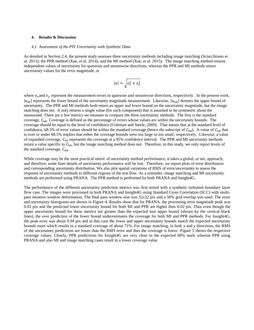
The performance of the different uncertainty prediction metrics was first tested with a synthetic turbulent boundary layer

flow case. The images were processed in both PRANA and Insight4G using Standard Cross Correlation (SCC) with multi-

pass iterative window deformation. The final pass window size was 32x32 pix and a 50% grid overlap was used. The error

and uncertainty histograms are shown in Figure 4. Results show that for PRANA, the processing error magnitude peak was

0.02 pix and the predicted lower uncertainty bound for both MI and PPR are higher than 0.02 pix. Thus even though the

upper uncertainty bound for these metrics are greater than the expected true upper bound (shown by the vertical black

lines), the over prediction of the lower bound underestimates the coverage for both MI and PPR methods. For Insight4G,

the peak error was about 0.04 pix and in this case the lower and upper uncertainty bounds match the expected uncertainty

bounds more which results in a standard coverage of about 71%. For image matching, in both x and y directions, the RMS

of the uncertainty predictions are lower than the RMS error and thus the coverage is lower. Figure 5 shows the respective

coverage values. Clearly, PPR predictions for Insight4G are very close to the expected 68% mark whereas PPR using

PRANA and also MI and image matching cases result in a lower coverage value.

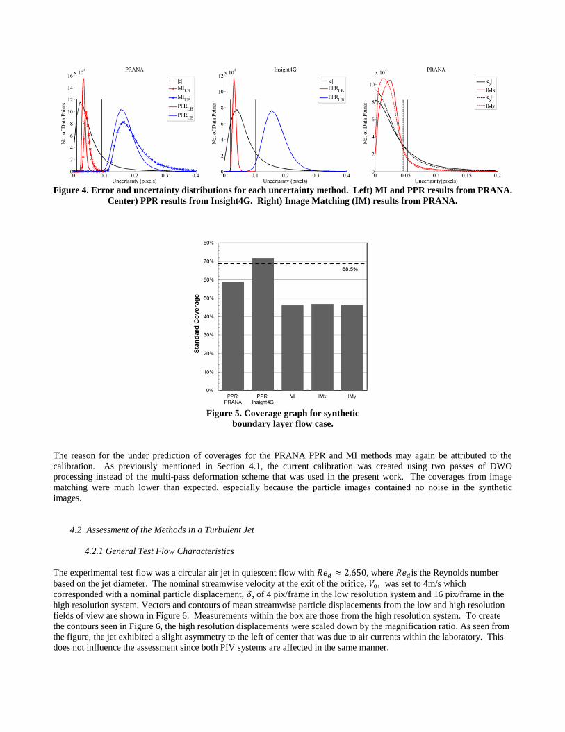
Figure 4. Error and uncertainty distributions for each uncertainty method. Left) MI and PPR results from PRANA.

Center) PPR results from Insight4G. Right) Image Matching (IM) results from PRANA.

Figure 5. Coverage graph for synthetic

boundary layer flow case.

The reason for the under prediction of coverages for the PRANA PPR and MI methods may again be attributed to the

calibration. As previously mentioned in Section 4.1, the current calibration was created using two passes of DWO

processing instead of the multi-pass deformation scheme that was used in the present work. The coverages from image

matching were much lower than expected, especially because the particle images contained no noise in the synthetic

images.

4.2 Assessment of the Methods in a Turbulent Jet

4.2.1 General Test Flow Characteristics

The experimental test flow was a circular air jet in quiescent flow with , where is the Reynolds number

based on the jet diameter. The nominal streamwise velocity at the exit of the orifice, , was set to 4m/s which

corresponded with a nominal particle displacement, , of 4 pix/frame in the low resolution system and 16 pix/frame in the

high resolution system. Vectors and contours of mean streamwise particle displacements from the low and high resolution

fields of view are shown in Figure 6. Measurements within the box are those from the high resolution system. To create

the contours seen in Figure 6, the high resolution displacements were scaled down by the magnification ratio. As seen from

the figure, the jet exhibited a slight asymmetry to the left of center that was due to air currents within the laboratory. This

does not influence the assessment since both PIV systems are affected in the same manner.

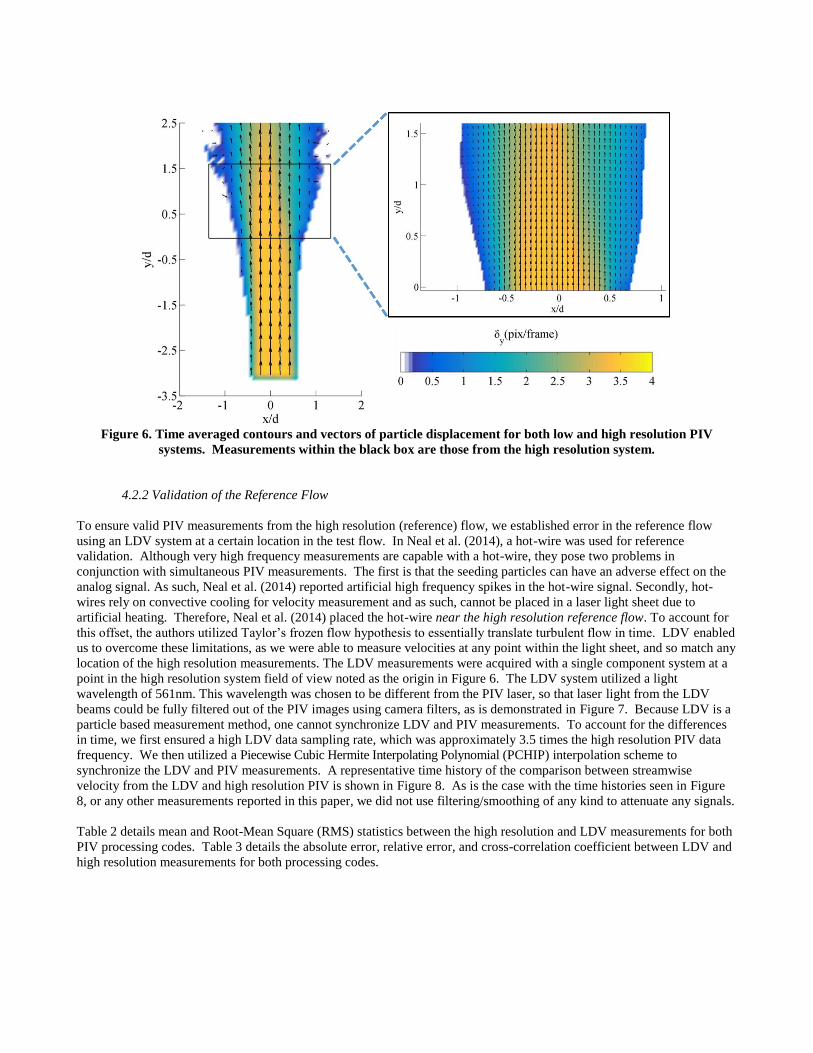
Figure 6. Time averaged contours and vectors of particle displacement for both low and high resolution PIV

systems. Measurements within the black box are those from the high resolution system.

4.2.2 Validation of the Reference Flow

To ensure valid PIV measurements from the high resolution (reference) flow, we established error in the reference flow

using an LDV system at a certain location in the test flow. In Neal et al. (2014), a hot-wire was used for reference

validation. Although very high frequency measurements are capable with a hot-wire, they pose two problems in

conjunction with simultaneous PIV measurements. The first is that the seeding particles can have an adverse effect on the

analog signal. As such, Neal et al. (2014) reported artificial high frequency spikes in the hot-wire signal. Secondly, hot-

wires rely on convective cooling for velocity measurement and as such, cannot be placed in a laser light sheet due to

artificial heating. Therefore, Neal et al. (2014) placed the hot-wire near the high resolution reference flow. To account for

this offset, the authors utilized Taylor’s frozen flow hypothesis to essentially translate turbulent flow in time. LDV enabled

us to overcome these limitations, as we were able to measure velocities at any point within the light sheet, and so match any

location of the high resolution measurements. The LDV measurements were acquired with a single component system at a

point in the high resolution system field of view noted as the origin in Figure 6. The LDV system utilized a light

wavelength of 561nm. This wavelength was chosen to be different from the PIV laser, so that laser light from the LDV

beams could be fully filtered out of the PIV images using camera filters, as is demonstrated in Figure 7. Because LDV is a

particle based measurement method, one cannot synchronize LDV and PIV measurements. To account for the differences

in time, we first ensured a high LDV data sampling rate, which was approximately 3.5 times the high resolution PIV data

frequency. We then utilized a Piecewise Cubic Hermite Interpolating Polynomial (PCHIP) interpolation scheme to

synchronize the LDV and PIV measurements. A representative time history of the comparison between streamwise

velocity from the LDV and high resolution PIV is shown in Figure 8. As is the case with the time histories seen in Figure

8, or any other measurements reported in this paper, we did not use filtering/smoothing of any kind to attenuate any signals.

Table 2 details mean and Root-Mean Square (RMS) statistics between the high resolution and LDV measurements for both

PIV processing codes. Table 3 details the absolute error, relative error, and cross-correlation coefficient between LDV and

high resolution measurements for both processing codes.

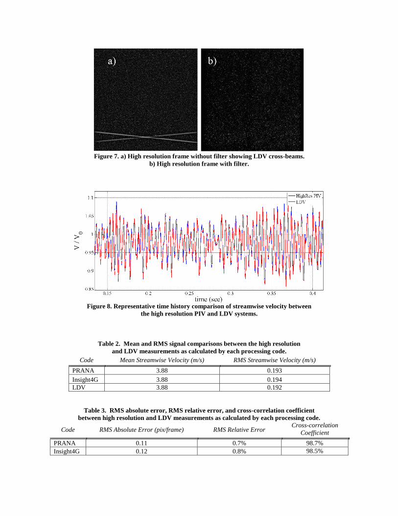
Figure 7. a) High resolution frame without filter showing LDV cross-beams.

b) High resolution frame with filter.

Figure 8. Representative time history comparison of streamwise velocity between

the high resolution PIV and LDV systems.

Table 2. Mean and RMS signal comparisons between the high resolution

and LDV measurements as calculated by each processing code.

Code Mean Streamwise Velocity (m/s) RMS Streamwise Velocity (m/s)

PRANA 3.88 0.193

Insight4G 3.88 0.194

LDV 3.88 0.192

Table 3. RMS absolute error, RMS relative error, and cross-correlation coefficient

between high resolution and LDV measurements as calculated by each processing code.

Code RMS Absolute Error (pix/frame) RMS Relative Error Cross-correlation

Coefficient

PRANA 0.11 0.7% 98.7%

Insight4G 0.12 0.8% 98.5%

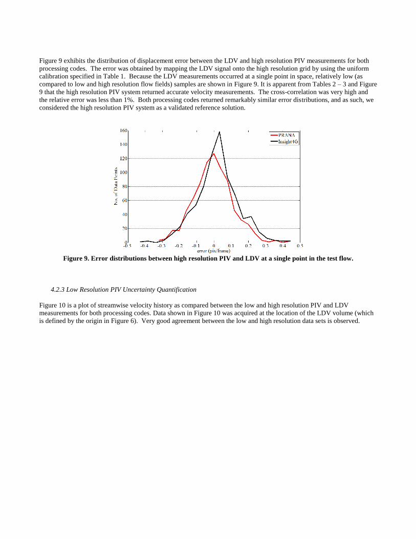
Figure 9 exhibits the distribution of displacement error between the LDV and high resolution PIV measurements for both

processing codes. The error was obtained by mapping the LDV signal onto the high resolution grid by using the uniform

calibration specified in Table 1. Because the LDV measurements occurred at a single point in space, relatively low (as

compared to low and high resolution flow fields) samples are shown in Figure 9. It is apparent from Tables 2 – 3 and Figure

9 that the high resolution PIV system returned accurate velocity measurements. The cross-correlation was very high and

the relative error was less than 1%. Both processing codes returned remarkably similar error distributions, and as such, we

considered the high resolution PIV system as a validated reference solution.

Figure 9. Error distributions between high resolution PIV and LDV at a single point in the test flow.

4.2.3 Low Resolution PIV Uncertainty Quantification

Figure 10 is a plot of streamwise velocity history as compared between the low and high resolution PIV and LDV

measurements for both processing codes. Data shown in Figure 10 was acquired at the location of the LDV volume (which

is defined by the origin in Figure 6). Very good agreement between the low and high resolution data sets is observed.

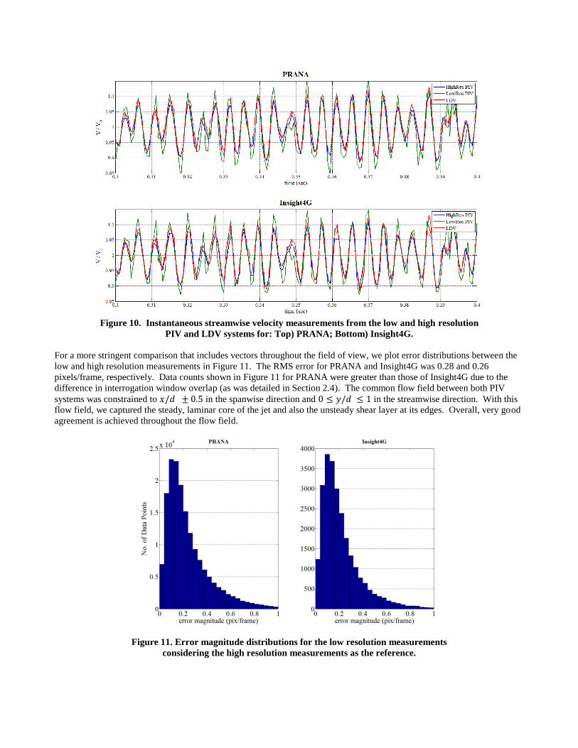
Figure 10. Instantaneous streamwise velocity measurements from the low and high resolution

PIV and LDV systems for: Top) PRANA; Bottom) Insight4G.

For a more stringent comparison that includes vectors throughout the field of view, we plot error distributions between the

low and high resolution measurements in Figure 11. The RMS error for PRANA and Insight4G was 0.28 and 0.26

pixels/frame, respectively. Data counts shown in Figure 11 for PRANA were greater than those of Insight4G due to the

difference in interrogation window overlap (as was detailed in Section 2.4). The common flow field between both PIV

systems was constrained to in the spanwise direction and in the streamwise direction. With this

flow field, we captured the steady, laminar core of the jet and also the unsteady shear layer at its edges. Overall, very good

agreement is achieved throughout the flow field.

Figure 11. Error magnitude distributions for the low resolution measurements

considering the high resolution measurements as the reference.

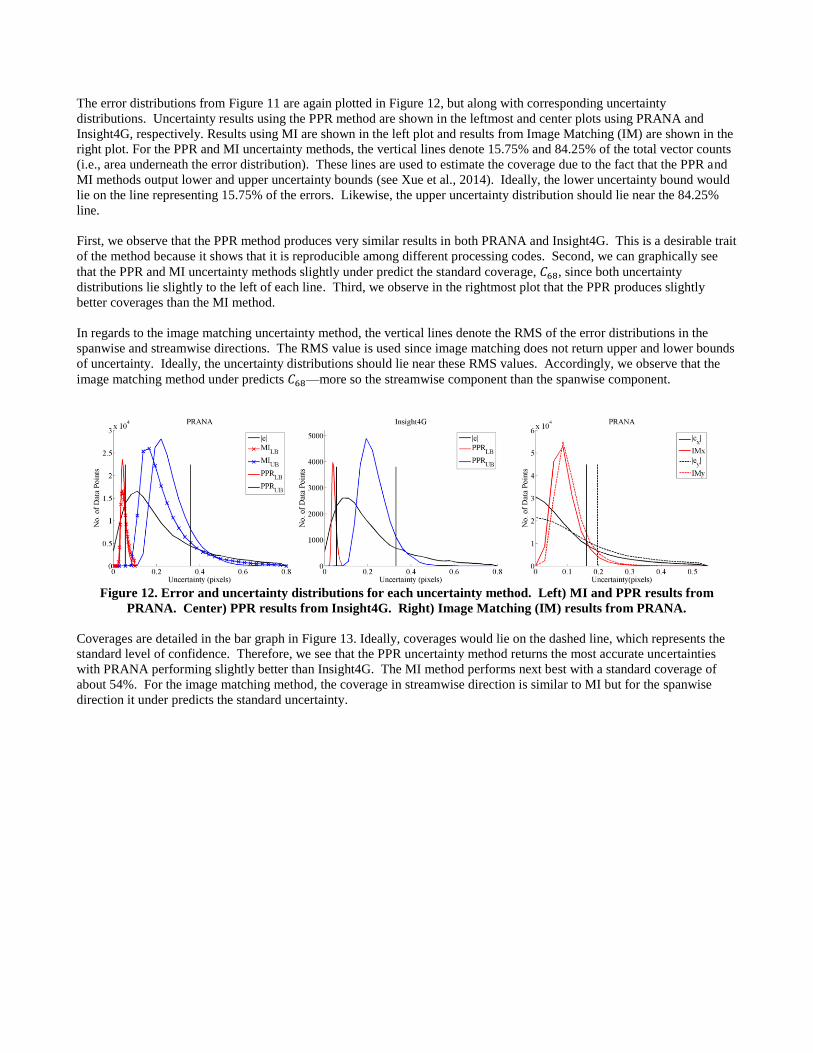
The error distributions from Figure 11 are again plotted in Figure 12, but along with corresponding uncertainty

distributions. Uncertainty results using the PPR method are shown in the leftmost and center plots using PRANA and

Insight4G, respectively. Results using MI are shown in the left plot and results from Image Matching (IM) are shown in the

right plot. For the PPR and MI uncertainty methods, the vertical lines denote 15.75% and 84.25% of the total vector counts

(i.e., area underneath the error distribution). These lines are used to estimate the coverage due to the fact that the PPR and

MI methods output lower and upper uncertainty bounds (see Xue et al., 2014). Ideally, the lower uncertainty bound would

lie on the line representing 15.75% of the errors. Likewise, the upper uncertainty distribution should lie near the 84.25%

line.

First, we observe that the PPR method produces very similar results in both PRANA and Insight4G. This is a desirable trait

of the method because it shows that it is reproducible among different processing codes. Second, we can graphically see

that the PPR and MI uncertainty methods slightly under predict the standard coverage, , since both uncertainty

distributions lie slightly to the left of each line. Third, we observe in the rightmost plot that the PPR produces slightly

better coverages than the MI method.

In regards to the image matching uncertainty method, the vertical lines denote the RMS of the error distributions in the

spanwise and streamwise directions. The RMS value is used since image matching does not return upper and lower bounds

of uncertainty. Ideally, the uncertainty distributions should lie near these RMS values. Accordingly, we observe that the

image matching method under predicts —more so the streamwise component than the spanwise component.

Figure 12. Error and uncertainty distributions for each uncertainty method. Left) MI and PPR results from

PRANA. Center) PPR results from Insight4G. Right) Image Matching (IM) results from PRANA.

Coverages are detailed in the bar graph in Figure 13. Ideally, coverages would lie on the dashed line, which represents the

standard level of confidence. Therefore, we see that the PPR uncertainty method returns the most accurate uncertainties

with PRANA performing slightly better than Insight4G. The MI method performs next best with a standard coverage of

about 54%. For the image matching method, the coverage in streamwise direction is similar to MI but for the spanwise

direction it under predicts the standard uncertainty.

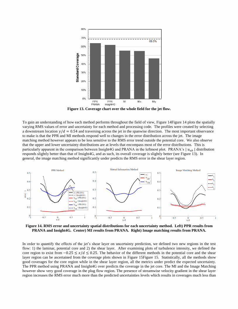
Figure 13. Coverage chart over the whole field for the jet flow.

To gain an understanding of how each method performs throughout the field of view, Figure 14Figure 14 plots the spatially

varying RMS values of error and uncertainty for each method and processing code. The profiles were created by selecting

a downstream location and traversing across the jet in the spanwise direction. The most important observance

to make is that the PPR and MI methods respond well to changes in the error distribution across the jet. The image

matching method however appears to be less sensitive to the RMS error trend outside the potential core. We also observe

that the upper and lower uncertainty distributions are at levels that encompass most of the error distributions. This is

particularly apparent in the comparison between Insight4G and PRANA in the leftmost plot. PRANA’s | | distribution

responds slightly better than that of Insight4G, and as such, its overall coverage is slightly better (see Figure 13). In

general, the image matching method significantly under predicts the RMS error in the shear layer region.

Figure 14. RMS error and uncertainty spatial distributions for each uncertainty method. Left) PPR results from

PRANA and Insight4G. Center) MI results from PRANA. Right) Image matching results from PRANA.

In order to quantify the effects of the jet’s shear layer on uncertainty prediction, we defined two new regions in the test

flow: 1) the laminar, potential core and 2) the shear layer. After examining plots of turbulence intensity, we defined the

core region to exist from . The behavior of the different methods in the potential core and the shear

layer region can be ascertained from the coverage plots shown in Figure 15Figure 15. Statistically, all the methods show

good coverages for the core region while in the shear layer region, all the metrics under predict the expected uncertainty.

The PPR method using PRANA and Insight4G over predicts the coverage in the jet core. The MI and the Image Matching

however show very good coverage in the plug flow region. The presence of streamwise velocity gradient in the shear layer

region increases the RMS error much more than the predicted uncertainties levels which results in coverages much less than

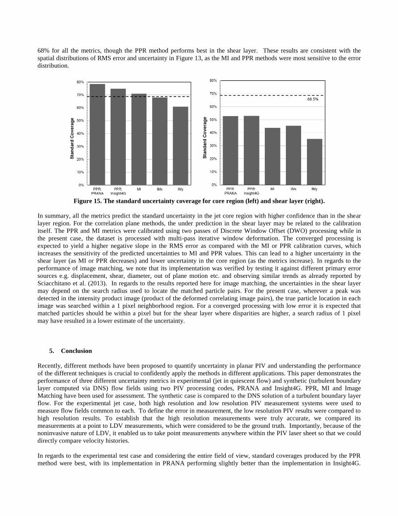
68% for all the metrics, though the PPR method performs best in the shear layer. These results are consistent with the

spatial distributions of RMS error and uncertainty in Figure 13, as the MI and PPR methods were most sensitive to the error

distribution.

Figure 15. The standard uncertainty coverage for core region (left) and shear layer (right).

In summary, all the metrics predict the standard uncertainty in the jet core region with higher confidence than in the shear

layer region. For the correlation plane methods, the under prediction in the shear layer may be related to the calibration

itself. The PPR and MI metrics were calibrated using two passes of Discrete Window Offset (DWO) processing while in

the present case, the dataset is processed with multi-pass iterative window deformation. The converged processing is

expected to yield a higher negative slope in the RMS error as compared with the MI or PPR calibration curves, which

increases the sensitivity of the predicted uncertainties to MI and PPR values. This can lead to a higher uncertainty in the

shear layer (as MI or PPR decreases) and lower uncertainty in the core region (as the metrics increase). In regards to the

performance of image matching, we note that its implementation was verified by testing it against different primary error

sources e.g. displacement, shear, diameter, out of plane motion etc. and observing similar trends as already reported by

Sciacchitano et al. (2013). In regards to the results reported here for image matching, the uncertainties in the shear layer

may depend on the search radius used to locate the matched particle pairs. For the present case, wherever a peak was

detected in the intensity product image (product of the deformed correlating image pairs), the true particle location in each

image was searched within a 1 pixel neighborhood region. For a converged processing with low error it is expected that

matched particles should be within a pixel but for the shear layer where disparities are higher, a search radius of 1 pixel

may have resulted in a lower estimate of the uncertainty.

5. Conclusion

Recently, different methods have been proposed to quantify uncertainty in planar PIV and understanding the performance

of the different techniques is crucial to confidently apply the methods in different applications. This paper demonstrates the

performance of three different uncertainty metrics in experimental (jet in quiescent flow) and synthetic (turbulent boundary

layer computed via DNS) flow fields using two PIV processing codes, PRANA and Insight4G. PPR, MI and Image

Matching have been used for assessment. The synthetic case is compared to the DNS solution of a turbulent boundary layer

flow. For the experimental jet case, both high resolution and low resolution PIV measurement systems were used to

measure flow fields common to each. To define the error in measurement, the low resolution PIV results were compared to

high resolution results. To establish that the high resolution measurements were truly accurate, we compared its

measurements at a point to LDV measurements, which were considered to be the ground truth. Importantly, because of the

noninvasive nature of LDV, it enabled us to take point measurements anywhere within the PIV laser sheet so that we could

directly compare velocity histories.

In regards to the experimental test case and considering the entire field of view, standard coverages produced by the PPR

method were best, with its implementation in PRANA performing slightly better than the implementation in Insight4G.

The PPR method produced consistent results between both processing codes, which is a desirable trait of its performance in

different processing environments. The MI performed next best, followed by image matching. When considering the

response of uncertainty calculations to varying error distributions, each method was able to match uncertainty and error in

the jet’s potential core, but in the shear layer, only the PPR and MI uncertainty methods really responded (albeit not as

much as it should have) to the increased error in measurement. Therefore, we separated the jet flow into two distinct

regions (potential core and shear layer regions) to quantify the effects of velocity gradients on each uncertainty method. In

the core, the MI and image matching methods performed best. In the shear layer region, the PPR method performed best.

With respect to the synthetic turbulent boundary layer, coverages from the PPR method as implemented in Insight4G were

best. This was followed by the PPR implementation in PRANA. MI and image matching showed similar coverage. The

cause for the under prediction in uncertainties for the correlation plane methods is likely due to calibration as current

metrics were determined from a DWO processing technique but the current study employed window deformation. The

cause for the significant under prediction by image matching is unknown, but it should be noted that great care was taken to

accurately implement the method following Sciacchitano et al. (2013).

References

Brady, M. R., Raben, S. G., & Vlachos, P. P. (2009). Methods for digital particle image sizing (DPIS): comparisons and

improvements. Flow Measurement and Instrumentation, 20(6), 207-219.

Charonko, J. J., & Vlachos, P. P. (2013). Estimation of uncertainty bounds for individual particle image velocimetry

measurements from cross-correlation peak ratio. Measurement Science and Technology, 24(6), 065301.

Coleman, H. W., & Steele, W. G. (2009). Experimentation, validation, and uncertainty analysis for engineers. John Wiley

& Sons.

Eckstein, A. C., Charonko, J., & Vlachos, P. (2008). Phase correlation processing for DPIV measurements. Experiments in

Fluids, 45(3), 485-500.

Eckstein, A., & Vlachos, P. P. (2009). Assessment of advanced windowing techniques for digital particle image

velocimetry (DPIV). Measurement Science and Technology, 20(7), 075402.

Eckstein, A., & Vlachos, P. P. (2009). Digital particle image velocimetry (DPIV) robust phase correlation. Measurement

Science and Technology, 20(5), 055401.

Fincham, A., & Delerce, G. (2000). Advanced optimization of correlation imaging velocimetry algorithms. Experiments in

Fluids, 29(1), S013-S022.

Huang, H., Dabiri, D., & Gharib, M. (1997). On errors of digital particle image velocimetry. Measurement Science and

Technology, 8(12), 1427.

Kähler, C. J., Scharnowski, S., & Cierpka, C. (2012). On the uncertainty of digital PIV and PTV near walls. Experiments in

fluids, 52(6), 1641-1656.

Li, Y., Perlman, E., Wan, M., Yang, Y., Meneveau, C., Burns, R.,& Eyink, G. (2008). A public turbulence database cluster

and applications to study Lagrangian evolution of velocity increments in turbulence. Journal of Turbulence, (9), N31.

Neal, D. R., Sciacchitano, A., Smith, B. L., & Scarano, F. (2015). Collaborative framework for piv uncertainty

quantification: the experimental database. Meas Sci Technol, 26.

Raffel, M., Willert, C. E., & Kompenhans, J. (2013). Particle image velocimetry: a practical guide. Springer.

Sciacchitano, A., Wieneke, B., & Scarano, F. (2013). PIV uncertainty quantification by image matching. Measurement

Science and Technology,24(4), 045302.

Sciacchitano A., Neal D, Smith, B, Warner, S., Vlachos, P., Wieneke, B., and Scarano, F. (2015). Collaborative framework

for PIV uncertainty quantification: comparative assessment ofmethods. Measurement Science and Technology. 26(7),

074004.

Timmins, B. H., Smith, B. L., & Vlachos, P. P. (2010, January). Automatic particle image velocimetry uncertainty

quantification. In ASME 2010 3rd Joint US-European Fluids Engineering Summer Meeting collocated with 8th

International Conference on Nanochannels, Microchannels, and Minichannels(pp. 2811-2826). American Society of

Mechanical Engineers.

Timmins, B. H., Wilson, B. W., Smith, B. L., & Vlachos, P. P. (2012). A method for automatic estimation of instantaneous

local uncertainty in particle image velocimetry measurements. Experiments in fluids, 53(4), 1133-1147.

Vlachos, P. (2015). http://sourceforge.net/projects/qi-tools/

Wieneke, B., & Prevost, R. (2014). DIC uncertainty estimation from statistical analysis of correlation values.

In Advancement of Optical Methods in Experimental Mechanics, Volume 3 (pp. 125-136). Springer International

Publishing.

Xue, Z., Charonko, J. J., & Vlachos, P. P. (2014). Particle image velocimetry correlation signal-to-noise ratio metrics and

measurement uncertainty quantification. Measurement Science and Technology, 25(11), 115301.

Xue, Z., Charonko, J. J., & Vlachos, P. P. (2015). Particle image pattern mutual information and uncertainty estimation for

particle image velocimetry.Measurement Science and Technology, 26(7), 074001.