Scholars' Mine Scholars' Mine

Masters Theses Student Theses and Dissertations

1972

An engineering analysis of fluid amplifiers and development of an An engineering analysis of fluid amplifiers and development of an

air velocity sensor air velocity sensor

Gian Sagar Aneja

Follow this and additional works at: https://scholarsmine.mst.edu/masters_theses

Part of the Mechanical Engineering Commons

Department: Department:

Recommended Citation Recommended Citation Aneja, Gian Sagar, "An engineering analysis of fluid amplifiers and development of an air velocity sensor" (1972). Masters Theses. 6715. https://scholarsmine.mst.edu/masters_theses/6715

This thesis is brought to you by Scholars' Mine, a service of the Missouri S&T Library and Learning Resources. This work is protected by U. S. Copyright Law. Unauthorized use including reproduction for redistribution requires the permission of the copyright holder. For more information, please contact scholarsmine@mst.edu.

l/

AN ENGINEERING ANALYSIS OF FLUID AMPLIFIERS

AND DEVELOPMENT OF AN AIR VEWCITY SENSOR

by

GIAN SAGAR ANEJA, 1948-

A

THESIS

Presented to the Faculty of the Graduate School of the

UNIVERSITY OF MISSOURI-ROLLA

In Partial Fulfillment of the Requirements for the Degree

MASTER OF SCIENCE IN MECHANICAL ENGINEERING

T2690 1972 130 pages

c.l

Approved by

ii

ABSTRACT

Fluidics, the new control techniqu~ finds its use amongst the

conventional electronics and pneumatics due to some of its impressive

features. Selected literature about bistable and proportional ampli­

fiers has been presented for better understanding of the element

behavior.

Sensors; typical applications of fluidics have been described

separately. An air flow velocity sensor has been set-up. Basically it

consists of a cylinder placed across the air flow that sheds vortices

in the wake due to 'Von Karman Vortex Street' phenomenon. The frequency

of vortices gives a measure of velocity. The velocities obtained from

the sensor have been compared to the ones obtained using a pitot tube.

iii

ACKNO\</LEIXlEMENTS

The author wishes to extend his sincere thanks and appreciation

to his advisor, Dr. D. A. Gyorog, for the guidance, encouragements

and valuable suggestions throughout the course of this thesis.

The author is grateful to Dr. V. J. Flanigon. His assistance

in reviewing the manuscript made this report possible.

iv

TABLE OF CONT~~TS

Page

ABSTRACT •••••••••••••••••••••••••••••••••••••••••••••••••••• ii

ACKNOWLEDGEMENTS ········•···········•··········••··········· LIST OF ILLUSTRATIONS ................•..•..•..•....••.•...•• LIST OF TABLES •..••.•...•.•••.....•.....•....••.•.•...•..•.• LIST OF SYMBOLS •••··••···•·•·•··•••·•······•·········•····••

I.

II.

III.

IV.

v. VI.

INTRODUCTION •···•·····•···•·•·•·················· BISTABLE AMPLIFIERS . ........•.....•..•.•......... A.

B.

. ..........•.••.•. Jet Attachment Amplifiere

Turbulence Amplifiere . •.................... PROPORTIONAL AMPLIFIERS ••••••••••••••••••••••••••

A.

B.

Jet Interaction Amplifiere . ............... . Vortex Amplifiere . ........................ .

FLUID SENSORS ••••••••••••••••••••••••••••••••••••

A.

B.

c.

D.

E.

Rotational Speed Measurement •••••••••••••••

Torque Meaeurement •••••••••••••••••••••·•••

Temperature Seneor and Control System ••••••

Liquid Level Sensor ••••••••••••••••••••••••

Air Flow Velocity Seneor •••••••••••••••••••

AIR FLOW VELOCITY SENSOR

S~~y AND CONCLUSIONS

. ..............•...•....• . ............•............

BIBLlOGRAPHY ••••••••••••••••••••••••••••••••••••••••••••••••

VITA ••••••••••••••••••••••••••••••••••••••••••••••••••••••••

iii

vi

xi

xii

1

5

5

28

37

37

63

70

70

72

73

76

76

78

100

103

106

TABLE OF CONTENTS (Continued)

APPENDICES • .••••••.•..•....••..•......•..•..•....•.•..••• A.

B.

EXPERIMENTAL DATA ••••••••••••••••••••••••••••••

DRAG FORCE AND VORTEX FREXtUENCY RELATION •••••••

v

Page

107

107

112

LIST OF ILLUSTRATIONS

Figure

1. A Wall Attachment Amplifier ••••••••••••••••••••••••••

2. A Jet Deflection Amplifier •••••••••••••••••••••••••••

Vortex Shedding Illustration •••••••••••••••••••••••••

vi

Page

3

3

3

4. (a) Output Characteristics of a Jet Attachment Amplifier. 7

(b) Supply Pressure and Flow Characteristics............. 7

5-

6.

7.

8. (a) (b) (c)

9.

10.

11.

12.

13.

14.

15.

16.

(a) (b) (c)

Typical Switching Characteristics Gf a Jet Attachment Amplifier............................................ 7 Terminated Wall or Bleed Type Switching.............. 10

Ccmtacting Both Walls Type Switching................. 10

Splitter Switching................................... 10 Short Splitter Distance Intermediate Splitter Distance Long Splitter Distance

Variation of Phase I Growth Time with Control Pu~se Strength••••••••••••••••••••••••••••••••••••••• 13

Variation of Switching Time with Control Pulse Strength............................................. 13 Basic Pattern of the Element......................... 15

Effect of the Vent Position on the Recovery Pressure. 15

Effect of the Terminal Crossing Angle on the Recovery Pressure.................................... 16

Effect of the Vent Width on the Recovery Pressure.... 16

Geometry of the Convex-Walled Amplifier.............. 18

Pressure Recovery vs. Normalized active-port flow for a convex walled amplifier for open and closed ports................................................ 19 Power Nozzle Velocity, V = 75 fps Power Nozzle Velocity, v: = 300 fps Power Nozzle Velocity, V6 = 460 fps

17. (a) Comfiguration of NASA Model 7 Fluid Jet Amplifier.... 21 (b) An Exploded View of the Fluid Amplifier.............. 21

Figure

18.

LIST OF ILLUSTRATIONS (Continued)

Control Pressures required to switch conventional and NASA Model 7 Fluid Amplifier into reverse flowing receivers. Other receiver is vented to

vii

Page

atmosphere........................................... 22 19. Superimposition of input-output characteristics

of Jet Attachment Amplifiers to test the cascading operation............................................ 24

20. Latched Vortex Vent Configuration as applied to a Fluid Amplifier.................................... 26

21. The Transition in the Power Jet of a Turbulence Amplifier on application of a control signal......... 30

22. A Generalized Turbulence Amplifier's input­output pressure curve showing operating range

23.

24.

25.

26. (a)

(b)

27.

28.

29.

30.

31.

32.

33.

and switching point.................................. 30

Input-Output Characteristics of a Turbulence Amplifier •••••••••••••••••••••••••••••••••••••••••••• 30

Determining the Fan-out capability of a Turbulence Amplifier •••••••••••••••••••••••••••••••••••••••••••• 33

A Fluidic Flip-Flop Device consisting of Turbulence Amplifiers........................................... 35

A Vented Jet Interaction Amplifier divided into three regions•••••••••••••••••••••••••••••••••••••••• 38 Simplified Block Diagram of Jet Interaction Amplifier •••••••••••••••••••••••••••••••••••••••••••• 38

Frequency Response Case I, Air Supply at 15 psi...... 42

Frequency Response Case II, Air Supply at 10 psi..... 42

Frequency Response Case III, Water Supply at 5 psi... 42

Characteristic pressure-flow curves for load circuit of Fluid Amp1ifier........................... 43

Pressure-flow Characteristics of control circuit of Fluid Amplifier...................................... 43

Superimposing load line on load circuit curves permits graphical solution........................... ~3

Input-Output Transfer Characteristics of Amplifier... 43

viii

LIST OF ILLUSTRATIONS (Continued)

Figure Page

34. Complete Electrical circuit equivalent for Jet Deflection Fluid Amplifier....................... 45

35. Simplification for low frequency signals............. 45

36. Simplification for high frequency signals............ 45

37. Frequency Response of actual circuit with response calculated from equivalent circuit.......... 47

38. Effect of variation in the Supply Pressure on Frequency Response of Fluid Amplifier................ 47

39. Gain Curves for a Proportional Center dump Amplifier corresponding to three different loads..... 49

4o. Frequency Response Characteristics corresponding to three different loads for the Proportional

41.

42.

43.

~- (a)

{b)

45.

%.

47.

~-

49.

~-

51. (a) (b)

Center dump Amplifier................................ 49

Jet Profiles for Various Deflections ••••••••••••••••• 51

Comparison of Theoretical and Experimental values of Gains••••••••••••••••••••••••••••••••••••••••••••• 52

Improved Proportional Amplifier...................... 54

Blocked Receiver gain Characteristics for a Single Amplifier..................................... 54

Blocked Receiver Characteristics for three-stage open loop Gain Block••••••••••••••••••••••••••••••••• 54

First Stage Output Characteristics................... 56

Second Stage Input Characteristics................... 56

Superimposition of Output-Input Characteristics...... 56

Possible mis-match detection while superimposition... 56

Matching operating points by Increasing Supply Pressure to the First Stage •••••••••••••••••••••••••• 58

Matching operating points by Reducing Supply Pressure to the Second Stage••••••••••••••••••••••••• 58

Effect of Shunt-Series Restricters on matching points 58 Location of Shunt-Series Restricters................. 58

ix

LIST OF ILLUSTRATIONS (Continued)

Figure Page

52. Matching Operating Ranges by adding Restrictors...... 58

5~. The Basic Fluidic Operational Amplifier.............. 60

54. FS-12 Summing Amplifier in J-79 Turbo-jet engine control••••••••••••••••••••••••••••••••••••••• 60

55. A Summing Amplifier's fluidic circuit................ 62

56. An Integrating Fluidic "Operational Amplifier Circuit. 62

57. Configuration of a Vortex Amplifier.................. 64

58. Physical Significance of exponent 'n'•••••••••••••••• 64

59. Characteristic curves for a commercially available vortex amplifier........................... 64

60. Effect of downstream pressure on output flow......... 64

61. (a) A Vortex Amplifier, Receiver and Vent on same side... 66 (b) Transfer Characteristics••••••••••••••••••••••••••••• 66

62. (a) A Vortex Amplifier, Receiver and Vent on opposite

(b) (c)

63.

64.

65.

66.

67.

68.

69.

70.

71.

72.

~ides•••••••••••••••••••••••••••••••••••••••••••••••• 66 Transfer Characteristics••••••••••••••••••••••••••••• 66 Effect of Vortex Amplifier Geometry on Recovery Pressure••••••••••••••••••••••••••••••••••••••••••••• 66

A Flow Control System................................ 68

A Fluidic Circuit for a Servo-Valve.................. 68

Rotational Speed Sensor using a Proportional Device.. 71

Rotational Speed Sensor using a Digital Device....... 71

Torque Sensor•••••••••••••••••••••••••••••••••••••••• 71

Proportional Temperature Control System.............. 74

Continuous Monitoring of Liquid Level................ 76

Pressure Distribution in a flow around a cylinder.... 79

A Stable Assymmetric Vortex Shedding Arrangement..... 79

strouhal No. vs. Reynolds No. for circular cylinders. 81

X

LIST OF ILLUSTRATIONS (Continued)

Figure Page

73. Drag coefficient for circular cylinders vs. Reynolds No.......................................... 83

74. (a) Vortex Sensor Tube set-up in the Wind Tunnel......... 87 (b) An Exploded View of the Vertex Sensor Tube •••••••••••• 88

75. A Plot of Strouhal No. vs. Reynolds No. corresponding to the Experimental Data on the Vortex Sensor•••••••••••••••••••••••••••••••••••••••• 93

76. A Plot of Pitot Tube Velocity and Vortex Frequency... 95

A1. Vortex Frequeacy Photograph corresponding to Test Run No.~2••••••••••••••••••••••••••••••••••••••• 110

A2. Vortex Frequency Photograph corresponding to Test Run No. 20 •••••••••••••••••••••••••••••••••••••• 110

B1. A Plot of Drag Force experienced by Sensor Tubes vs. Square of the Vortex Frequency ••••••••••••••••••••••• 114

xi

LIST OF TABLES

Table Page

I Evaluation of Strouhal Numbers and Reynolds Numbers for various experimental data•••••••••••••••••••••••• 90

II Percentage Uncertainties in Strouhal Number and and Reynolds Number•••••••••••••••••••••••••••••••••• 92

III Comparison of Pitot tube velocities and the velocities obtained from the plot of pitot tube velocity vs. vortex frequency..................................... 96

IV Comparison of Vortex Sensor velocities and the velocities obtained from the plot of pitot tube velocity vs. vortex frequency........................ 97

V Vortex Frequency and Pitot tube velocity Measurements 108

VI Pitot tube data •••••••••••••••••••••••••••••••••••••• 111

VII Evaluation of Drag Force experienced by the Sensor tubes•••••••••••••••••••••••••••••••••••••••••••••••• 113

VIII Evaluation of distance between free vortex layers for the Sensor tubes ••••••••••••••••••••••••••••••••• 116

A

A,B

c

c

d'

e

f

D

h

k

K

1

L

M

0

p

Q

r

R

LIST OF SYMBOLS

area

correspond to the two ports of an amplifier (control or the output)

control ports

capacitance of a fluid line

coefficient of drag

diameter of sensor tubes

distance between free vortex layers

ambient condi tiona

frequency of vortices shed

drag force

depth of channels for the fluid elements

xii

ratio of control nozzle width to power nozzle width

ratio of control mass flow to power mass flow

amplification factor

feedback cavity length for a fluidic oscillator

inductance of a fluid line

momentum of a fluid jet

receivers of fluid amplifiers

pressure

static pressure in the wind tunnel test section

dimensionless control flow

volume flow

radii of the latched vortex vent

resistance of a fluid line

R e

s

s

t

T

u

u

v

w

X,Y

x,'Y X

8

X v

z

v

e

't

LIST OF SY11BOLS (Continued)

Reynolds Number

laplace operator s-domain

Strouhal Number

thickness of the power nozzle width of fluid amplifiers

temperature

transport time

velocity of vortices with respect to the :t'l.owing liquid

tangential velocity in vortex chamber of vortex amplifier

vent width for a jet attachment amplifier

velocity of air flow

weight flow of fluid

rectangular coordinates

dimensionless rectangular coordinates

splitter location

vent location

impedence of a fluid line

control pulse strength

ratio of specific heats

jet deflection angle

time conl!Stant

deneity of air

viscosity of air

vent terminal crossing angle

uncertainty

xiii

I INTRODUCTION

Fluidic devices are being used as a new mode of control similar

to electronics and pneumatics. Active research in Fluidics started

with initiation by Harry Diamond Laboratories in 1960. Basically all

the technologies depend on a medium to transmit energy which in case

of Fluidics is gases e.g., air and liquids also are equally useful.

There are fluidic control components such as bistable amplifiers,

proportional amplifiers; elements such as resistors, capacitors and

devices such as O~NOR, AND/NAND; all these components find similar

use to the ones employed in electronic circuits.

1

T.he fluidic control applications have been growing rapidly

because of their impressive features such as higher reliability,

lower cost of production, environmental tolerance, reducing the

number of transducers etc. Fluidic applications include liquid level

sensing, temperature sensing, rotational speed measurement and object

sensing. It has also been used for process control, steam turbine

speed control, hydrofoil lift control, aircraft pitch rate damper

and fluid transmission control for diesel locomotive. Recently, fluid

operational amplifiers have also been developed. The limitations of

the fluidic components are slow response, noise problem, filtration

of supply flow, load sensitivity, difficulty in cascading, thereby

limiting the design of complicated circuits. In modern control

techniques, Fluidics has come to stay with electronics and pneumatics

and there has to be a compromise in their respective use as none of

them is perfect in itself when economic considerations are included

with the design considerations.

Out of the many fluidic components bistable and proportional

2

amplifiers play an active role in Fluidics. Wall attachment amplifier

and turbulence amplifier, both come under bistable amplifiers.

Similarly, under proportional amplifiers, there come jet deflection

(interaction) and vortex amplifiers.

Wall attachment amplifier is basically an application of the

Coanda Effect. If a jet of fluid, coming out of a nozzle, finds a

straight or curved wall with in a certain range of distance, the jet

attaches to the wall (Fig. 1) and travels along it. Switching it to

the opposite wall is done through a low pressure control input. If

the jet is again stable in the new position, the element is called

a bistable amplifier. T.he two output pressures could be recovered

separately by inserting a splitter in the downstream flow. On the

other hand if there are no Coanda Walls by the side of the power

jet (Fig. 2), it deflects on interaction with the control jet.

The output from the amplifier depends on the strength of the control

signal prior to saturation. Literature has been cited in the

following chapters, to furnish more details about bistable and

proportional amplifiers. Different types of switching, switching

time analysis, special design configurations and cascading amplifiers

have been dicsussed for jet attachment amplifiers. Tb analyse a jet

interaction amplifier a lumped parameter technique and an equivalent

electrical circuit has been presented. Also included are the design

steps for cascading amplifiers and development of an operational

amplifier and its applications in fluidic control circuits.

Different fluid sensors have been described and their practical

design feasibilities considered. The primary object of the present

Power Nozzle

Fig. 1.

p s

Fluid

Fig. 3.

Separation ubble

A Wall Attachment Amplifier

Interaction Region

cB

A Jet Deflection Amplifier

A Cylinder

Vortex Shedding Illustration

Output Flow

3

4

investigation was to analyse 'An Air Flow Velocity Sensor' and test

it experimentally. The principal behind this sensor is that a

cylinder immersed in an air flow sheds vortices in its wake (Fig. 3)

due to 'Von Karman Vortex Street', the frequency of vortices shed

gives a measure for the velocity of air flow.

5

II BISTABLE J'J,IPLIFIERS

An element, which gives two discrete levels of amplified output

on application of relatively small input signal, is known as a

bistable amplifier.

There are different fluidic components such as jet attachment

amplifiers, turbulence amplifiers, induction amplifiers which all

come under bistable amplifiers. In this chapter jet attachment and

turbulence amplifiers have been described with reference to available

literature.

A. Jet Attachment Amplifiers

It has already been mentioned in the Introduction that the

operation of a jet attachment amplifier is based on the Coanda Effect.

A fluid jet exiting a nozzle entrains the surrounding air. Due to a

free replacement of air surrounding the jet, there is no pressure

gradient set up across the jet. However, the presence of a wall

restricts the replacement of the entrained air and results in a drop

in pressure in the region. Thus, the jet leans towards the wall

forming a small low pressure separation bubble. This phenomenon was

historically found by Henry Coanda, a Rumanian Engineer. In the case

of no control flow, the power jet attaches to one of the walls at

random and remains stable. On application of a low pressure control

flow, the pressure in the separation bubble increases and the power

jet eventually detaches and flips to the other wall forming a new

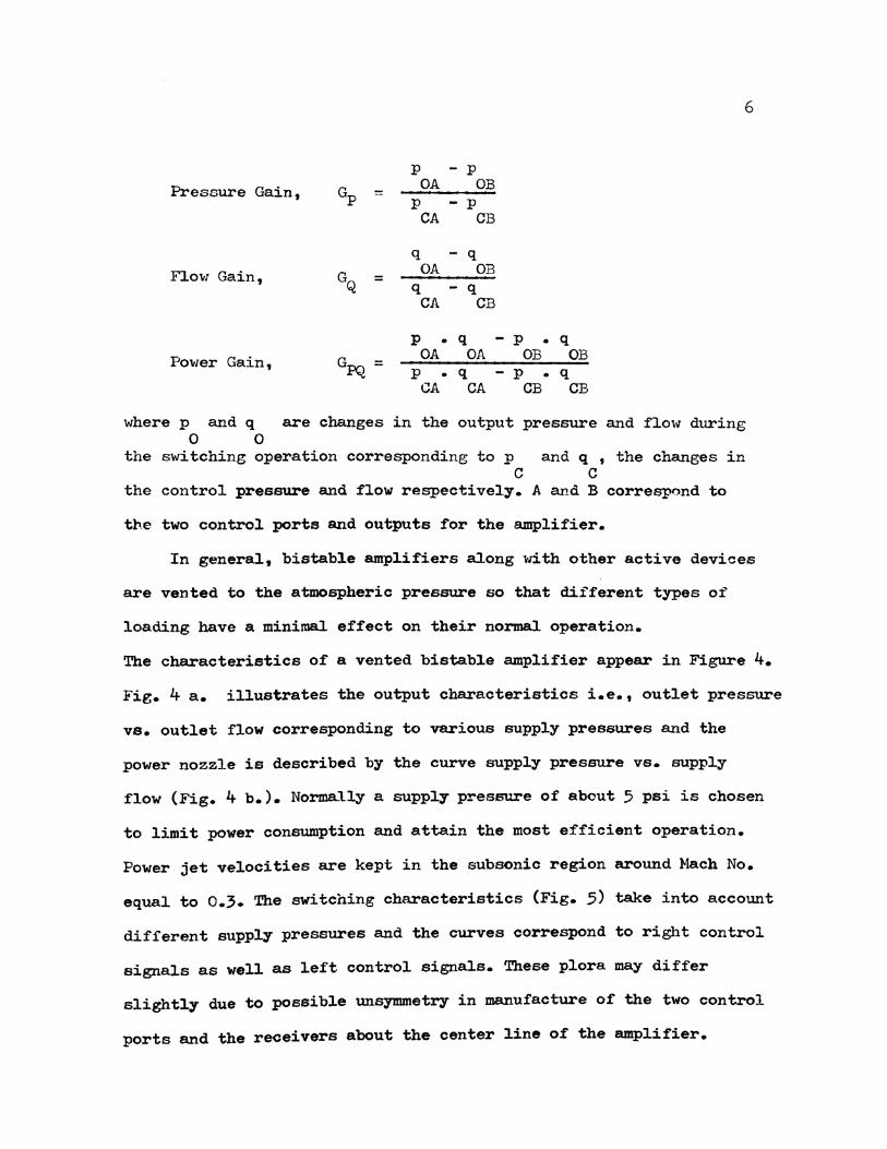
separation bubble. There are three kinds of switching gains for the

amplifier which are defined as follows;

6

p - p

Pressure Gain, :::: OA OB

p - p CA CB

q - q OA OB

q - q Flow Gain, =

CA CB

p • q - p • q OA OA OB OB

p • q - p • q Power Gain, GPQ =

CA CA CB CB

where p 0

andq 0

are changes in the output pressure and flow during

the switching operation corresponding to p and q , the changes in c c

the control pressure and flow respectively. A and B correspond to

tl'l.e two control ports and outputs for the amplifier.

In general, bistable amplifiers along ~dth other active devices

are vented to the atmospheric pressure so that different types of

loading have a minimal effect on their normal operation.

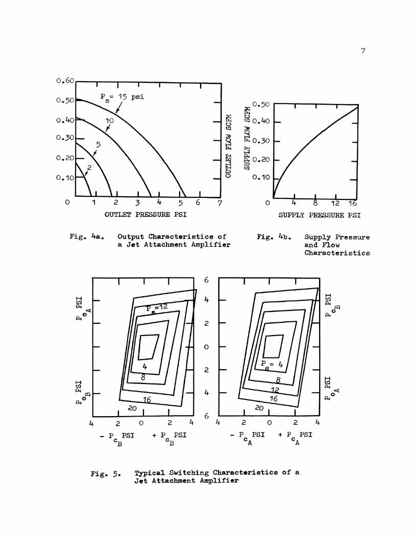
The characteristics of a vented bistable amplifier appear in Figure 4.

Fig. 4 a. illustrates the output characteristics i.e., outlet pressure

vs. outlet flow corresponding to various supply pressures and the

power nozzle is described by the curve supply pressure vs. supply

flow (Fig. 4 b.). NormaLly a supply pressure of about 5 psi is chosen

to limit power consumption and attain the most efficient operation.

Power jet velocities are kept in the subsonic region around Mach No.

equal to 0.3. The switching characteristics (Fig. 5) take into account

different supply pressures and the curves correspond to right control

signals as well as left control signals. These plora may differ

slightly due to possible unsymmetry in manufacture of the two control

ports and the receivers about the center line of the amplifier.

0

Fig.

7

~0-50

~ 0

0 tf.l o.4o

tf.l ::?!=

~ ~0.30 ~

~ ~ 0.20 l=l

l=l tf.l

0 0.10

1 2 3 5 7 0

OUTLET PRESSURE PSI SUPPLY PRESSURE PSI

4a. Output Characteristice of Fig. 4b. a Jet Attachment Amplifier

6

4

2

0

2

4

6 4 2 0 2 4 2 0 2

p PSI + p PSI - p PSI + p cB CB CA cA

Fig. 5· T,ypical Switching Characteristics of a Jet Attachment Amplifier

Supply Pressure and Flow Characteristics

H til A4p:j

A4 0

H

re< A40

4

PSI

8

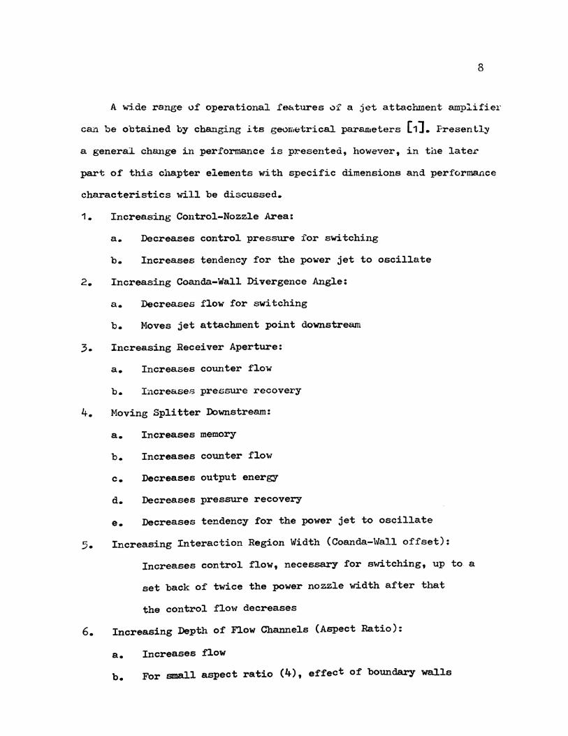
A -..."ide range of operational features .:>f a jet attaclunent ampli£ie1·

can be obtained by changing its georr.etrical parameters (1]. Fresently

a genera~ change in performance is presented, however, in the later

part of this clUlpter elements with specific dimensions and performance

characteristics will be discussed.

1. Increasing Control-Nozzle Area:

a. Decreases control pressure for switching

b. Increases tendency for the power jet to oscillate

2. Increasing Coanda-Wall Divergence Angle:

a. Decreases flow for switching

b. Moves jet attachment point downstream

3. Increasing Receiver Aperture:

a. Increases counter flow

b. Increases pressure recovery

4. Moving Splitter Downstream:

a. Increases memory

b. Increases counter flow

c. Decreases output energy

d. Decreases pressure recovery

e. Decreases tendency for the power jet to oscillate

5. Increasing Interaction Region Width (Coanda-Wall offset):

Increases control flow, necessary for switching, up to a

set back of twice the power nozzle width after that

the control flow decreases

6. Increasing Depth of Flow Channels (Aspect Ratio):

a. Increases flow

b. For small aspect ratio (4), effect of boundary walls

increases

7. Increasing Load:

a. Reduces control necessary for switching out of load

b. Increases control necessary for switching into load

c. Increases tendency for the power jet to oscillate

Switching is one of the most important aspects of a bistable

9

ampli£ier yet to be analysed in detail. Several authors have tried to

analyse the problem mathematically, worked with different configurations

to get an efficient switching mechanism. First of all a theoretical

description is given by Warren [2] , where it is classified in to

three types;

1. The two side walls terminate or have bleeds to separate the rest

of the wall {Fig. 6). On application of control flow the separation

bubble communicates with the atmospheric pressure through the

bleed. The main jet straightens up, with continued control flow

and entrainment of fluid on the other side causes the jet to

switch to the other wall. This type of switching is called

Terminated Wall or Bleed Type Switching.

2. In Contacting Both Walls type switching, the side walls are so

close that on application of control flow the power jet contacts

the opposite wall while still in contact with the first wall,

forming two separation bubbles {Fig. 7). This happens before the

power jet contacts the splitter. The first separation bubble grows

in size as the pressure increases due to the control flow.

Ultimately, the jet switches to the other side and switching is

completed when the opposite separation bubble reaches its

equilibrium state. In this type of switching the attachment walls

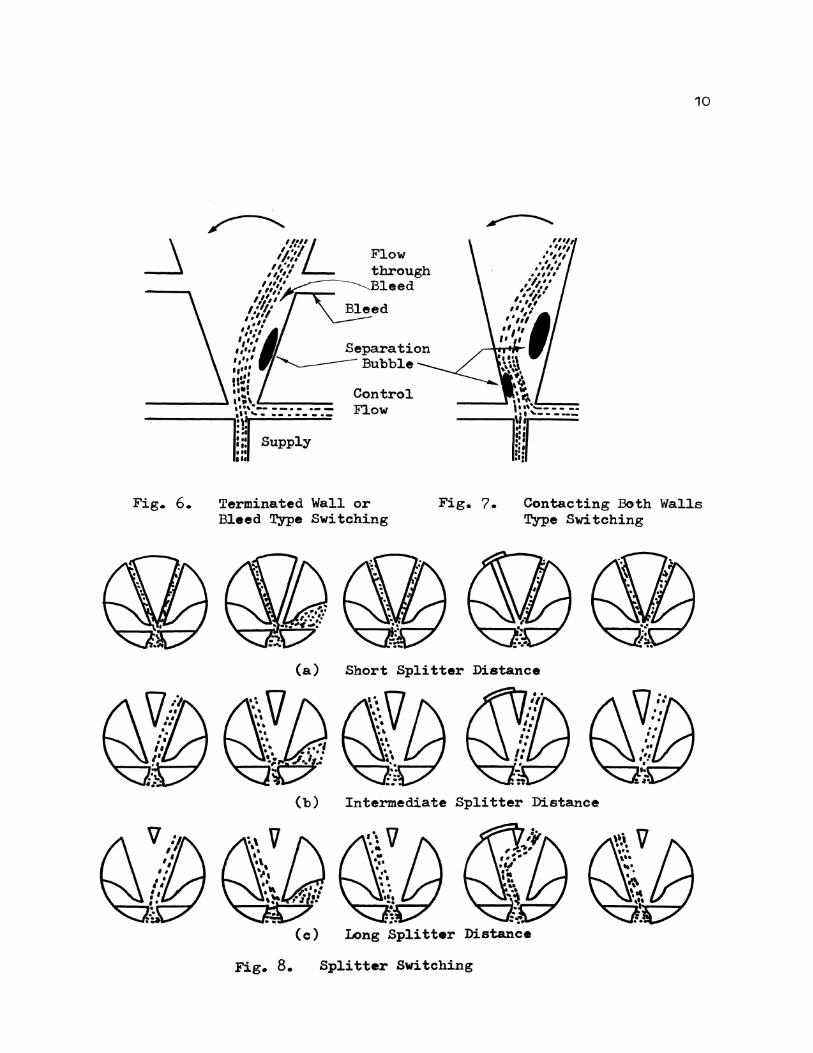
Fig. 6.

Flow through leed

Separation ...........____ Bubble

Control Fl. ow

10

Terminated Wall or Bleed Type Switching

Fig. 7. Contacting Both Walls Type Switching

(a) Short Splitter Distance

.. .. ~· ... , ~e;:.:

(b) Intermediate Splitter Distance

(c) Long Splitter Distance

Fig. 8. Splitter Switching

are relatively long and there is limited communication of the

separation bubble with the ambient pressure. However the pressure

in the separation bubble is of course less than on the unattached

side.

11

3. Splitter switching differs from the previous types in the sense

that the power jet reaches the splitter before touching opposite wall.

This occurs while the jet is contact with the first wall or in other

words, there is a splitter penetration before the jet contacts the

opposite wall or the separation bubble communicates with the atmos­

phere. If the splitter is located at the exit of the power nozzle,

a situation similar to a pipe flow occurs and the flow is split

equally in two channels (Fig. 8 a.). Control flow switches the power

jet but only when it is present and so is the effect of blocking one

of the outputs of the amplifier. Locating the splitter downstream

(Fig. 8 b.) decreases gain and increases stability of the jet. Effects

of splitter location further downstream as well as blocking one of the

outputs have been shown in Fig. 8 c.

To make a rough judgement about the type of switching for an

amplifier considering its geometrical parameters only, following

procedure is adopted. If the wall divergence angle is more than 15•

and they are located more than twice the power nozzle width apart and

then if the bleed vents are located downstream of splitter, the switching

is splitter type or if the bleed vents are located in the unstream,

the switching wi~ be terminated wall or bleed type. In the third case

if the wall divergence angle is less than 10oand they are located less

than twice the power nozzle width, further if the bleed vents and

splitter locations are downstream (more than 12 times the power nozzle

width), the type of switching will be contacting both walls type.

The switching time analysis on a large scale model [3] was a

special case to the amplifiers (Fig. 12) tested by Hara, Ozaki and

Harda [5]. It is claimed that the present model could be scaled

12

down from a 111 power nozzle throat width to a throat width of 0.04".

The Mach No. is limited to 0.3 and minimum Reynolds No. 104.

The switching time has been divided into three phases out of which

the third phase is usually omitted.

1. Bubble growth

2. Flipping power jet to opposite wall

3. Bubble shrinkage

Lush [ 3] extended the theory by Barque and Newman [4] by

describing the bubble growth in terms of the net flow into the

separation bubble, taking into account the control flow and assuming

quasi-steady flow conditions. Flipping time is essentially controlled

by the control pulse strength. It is recommended for the control flow

to be about twice the threshold value of flow calculated fow switching

that is how the dwell time is reduced. The test were made on a large

scale table model amplifier with 1" throat width (Fig. 12), throat

velocity of 170 fps and Reynolds No. 9X1o4• In the plots following

variables have been used.

Non-dimensional control flow

Non-dimensional time defined as:

Mean main jet velocity at nozzle exit X time Throat width

p = Main jet deflection which is proportional to the control

pulse strength or the control flow

0

0

0

0 0

00 0 8 0

0 00

• - • •• 0 .05 • 10 .15

Phase I Phase I Phase I Control Time

0

•

Theor·~----

Time 0 Time less -• Pulse Rise

0

0

•

0

•

.20 .25 .30 .35 CONTROL PULSE STRENGTH

Fig. 9. Variation of Phase I Growth Time with Control Pulse Strength

800

600

Phase I+II 0 Theory /

Total Switching~· Time /

Total Switching Time less Dwell Time

~0

13

0 0 -35

CONTROL PUlSE STRENGTH

Fig. 10. Variation of Switching Time with Contrel Pulse Strength

14

Figure 9 shows the variation of phase I growth time with control

pulse strength. The theoretical prediction~which do not include the

finite control pulse time, don't agree with experimental data. If

this time is subtracted from the experimental switching times, there

seems to be a good agreement in the results.

In the second plot (Fig. 10) the time ordinate includes the

flipping time of the jet. The dwell time is a maximum for control

pulse strength P= 0.09 and decreases to nearly zero at P= 0.3.

There is discrepancy in the results even when the dwell time is

subtracted from the experimental points. This has been explained as

the resulting inertia of the output columns of fluid can not be

neglected, as was assumed, thereby the probes set up in the outputs

measure longer time. Also, there is some effect due to the presence

of opposite wall that helps in switching. Considering these points,

the switching time estimates could be more precise.

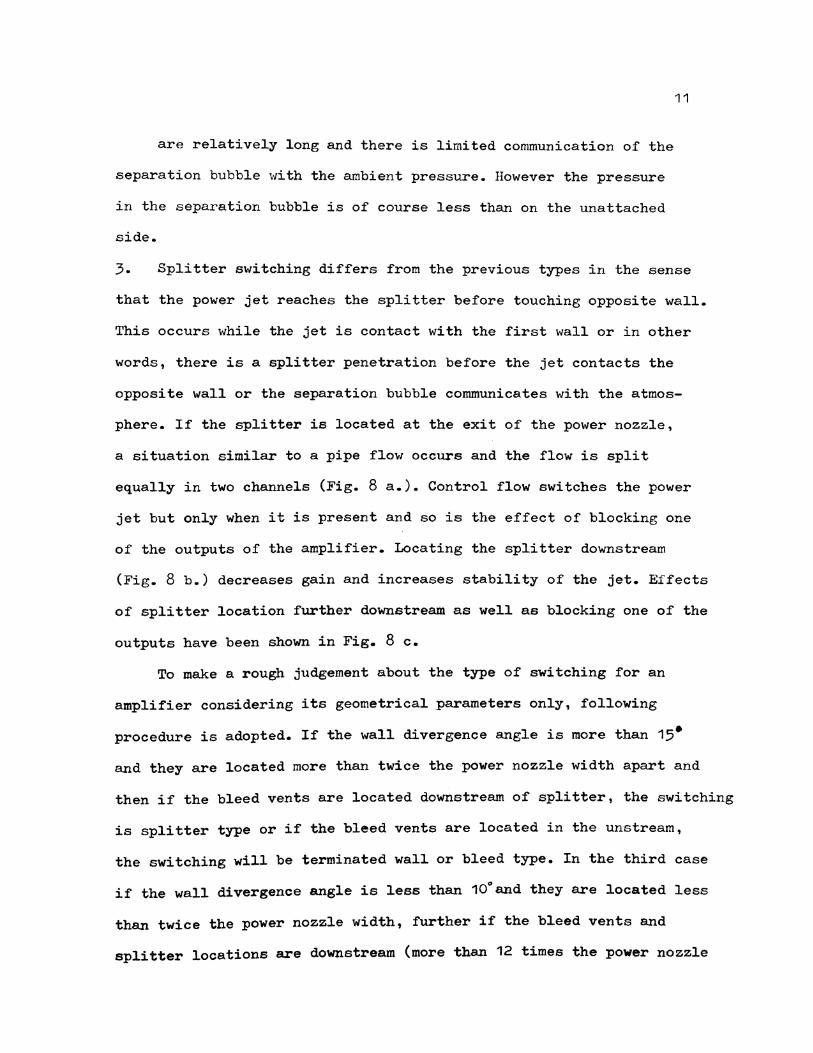
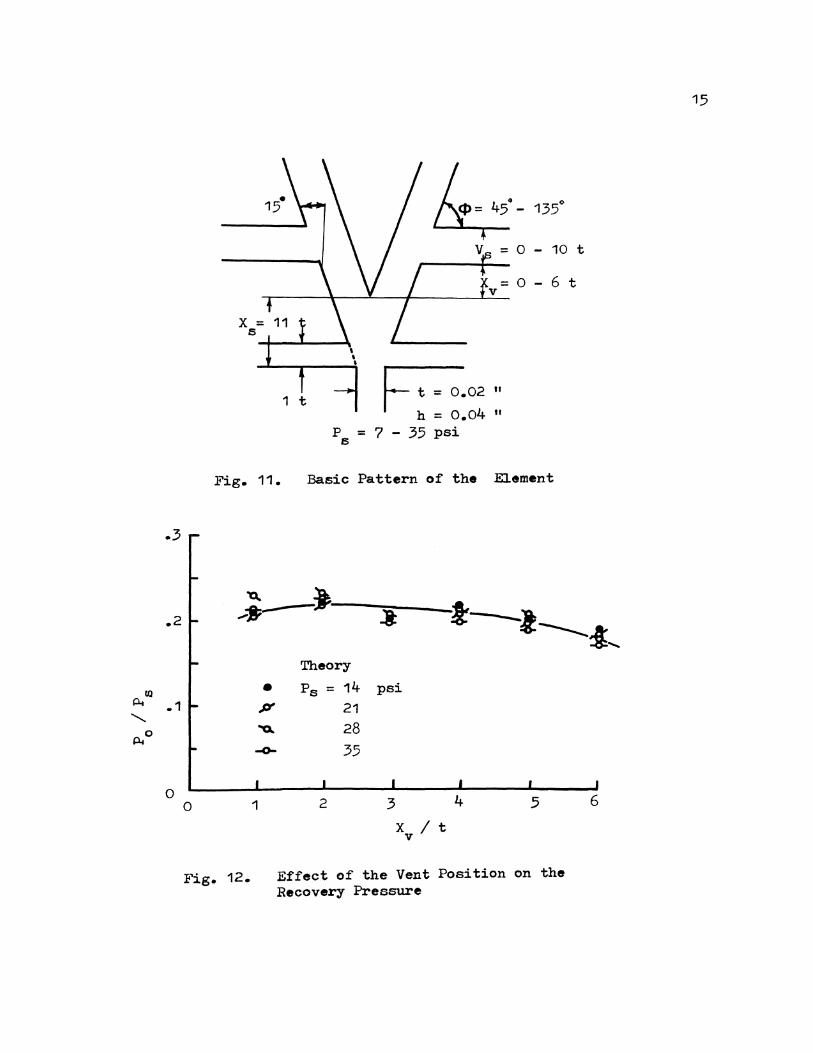
More experimental tests on an amplifier (Fig. 11), geometrically

similar to the one used by Lush (3] but smaller in size (0.02" power

nozzle width), were done by Harda, Ozaki and Hara [5] . Primarily

the analysis is aimed to investigare the effect of changing various

geometrical parameters on pressure recoveries. It was found that

recovery is not much effected by the vent position in case it is

located downstream of the splitter (Fig. 12), however it increases by

increasing the terminal crossing angle q>(Fig. 13). Increasing the

terminal angle is equivalent to closing the vent opening out of the

way to receiver, that is how the recovery pressure increases. It is

normally kept in the range of 75°- 90°. Also shown is the effect of

• 3

.2

.1

0

X = 5

1 t F-02" h = o.o4 "

P = 7 - 35 psi 5

10 t

- 6 t

Fig. 11 • Basic Pattern of the Element

'Q.

.... ~-

Theory

• Ps == 14 psi

JY 21 "'0.. 28 -o- 35

0 1 2 3 5

X It v

Fig. 12. Effect of the Vent Position on the Recovery Pressure

15

6

.3

(Q

~ .2

" ~0 .1

0

Theory

• p = 14 psi • s • .,#'

.P' 21 4 .:&. ""0.. 28 ~ 35

TERMINAL CROSSING ANGLE q>

Fig. 13. Effect of the Terminal Crossing Angle on the Recovery Pressure

~ .P' -« -31 • ""0.. Theory ~

-o- p = 14 psi • s .P' 21 'o... 28

m-2 -o- 35 ~ • " ~

~0 ~ ~ -&-;&< ~ .1

>E(

0 0 8 10

VENT WIDTH v s I t

Fig. 14. Effect of the Vent Width on the Recovery Pressure

16

changing vent width. It plays quite a dominating role. Considering

the experimental data and theoretical predictions, although they

don't agree (Fig. 14), it is obvious that the pressure recovery

17

drops considerably when the vent width exceeds twice the power nozzle

width.

Most of the work on jet attachment amplifiers deal with elements

having straight Coanda walls. Sarpkaya [6] tested three kinds of walls

straight, concave and convex, to determine whether it was possible to

have an improved performance by suitably curving the Coanda walls.

Concave walls revealed poor pressure recovery curves due to a

significant loss in energy due to turbulence mixing which dominates

over the loss due to wall friction. Also, the pressure recovery depends

on the size of the separation bubble to a large extent. In case of

convex walls the separation bubble is smaller in size and overall loss

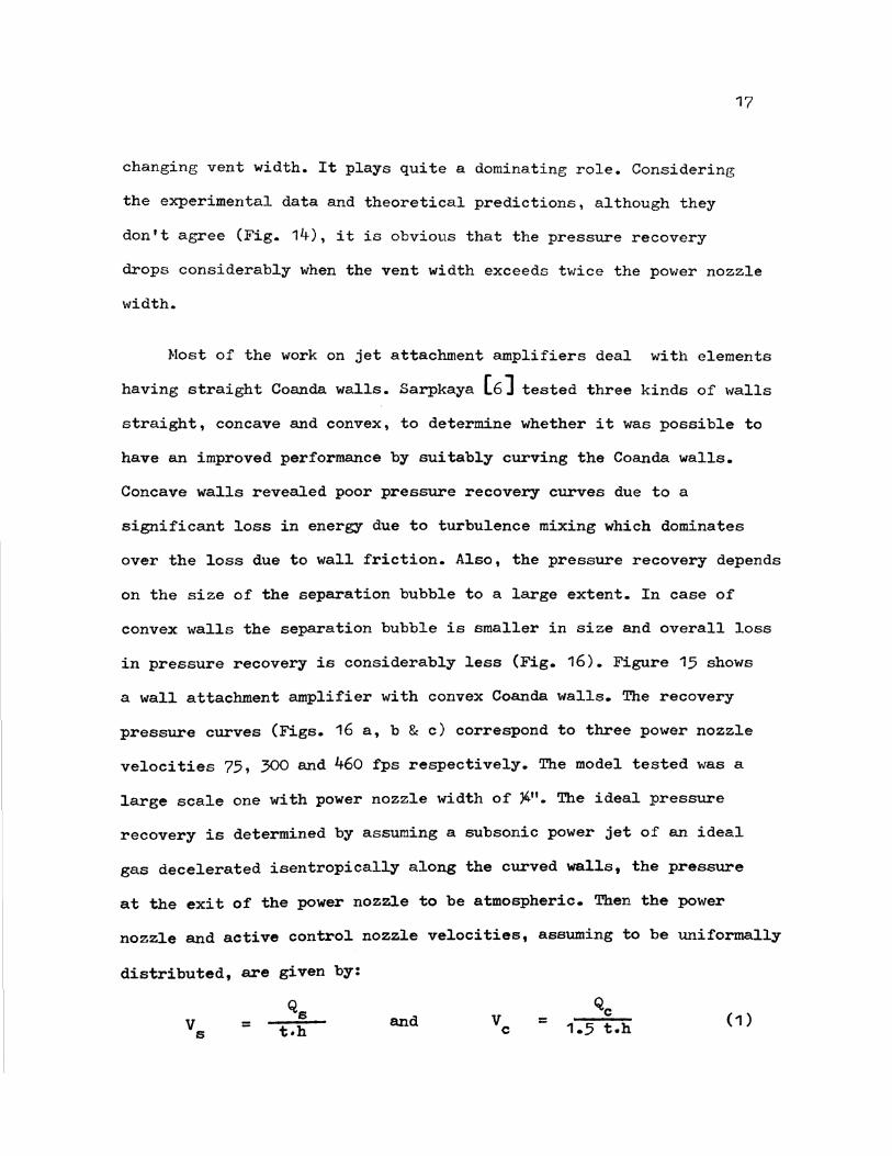
in pressure recovery is considerably less (Fig. 16). Figure 15 shows

a wall attachment amplifier with convex Coanda walls. The recovery

pressure curves (Figs. 16 a, b & c) correspond to three power nozzle

velocities 75, 300 and 460 fps respectively. The model tested was a

large scale one with power nozzle width of ~". The ideal pressure

recovery is determined by assuming a subsonic power jet of an ideal

gas decelerated isentropically along the curved walls, the pressure

at the exit of the power nozzle to be atmospheric. Then the power

nozzle and active control nozzle velocities, assuming to be uniformally

distributed, are given by:

= and v c = 1.5 t.h (1)

Fig. 15. Geometry of the Convex-Walled Amplifier

18

Vented Amplifier (open ports ......... "· ·•• Vented Ampli:fier

···-A·... '· ·.'4 (closed ports) ..... ' ·. \ . Eq. (3) , ... ,~.~

Unvented ~~ Unve~t~d Amplifier ~S. Ampl~f~er (open ports) ~ Closed

~0· ~ 9 . ~ .

\

~ . . ~

19

·-- ..... . ........ ~'-

~ ... •"-.. ........ , ... ....

-·----A.. ' .. ... .,.. .'-.,\ ... '~ ·~ -~

~ ~ ~ . . , \ ~ . -~ ..

q . . .3 Qo/Qs . • ~ •

• 20 .2 .2 .4 .6 .8 1.0 1.0

(a) v = 75 fps s

.9

.8

.7

.6

.5 (c) v = 460 fps

s .4

.3

.2 0

Fig. 16. Pressure Recovery vs. Normalized active-port flow for a convex walled amplifier for open and closed ports.

. • •

20

where 't' is the power nozzle width and 'h' is the depth of the

element channels. Making use of the Bernoulli's equation and ignoring

the energy

p = s

correction !actors;

P v 2 PV 2 • s • 0

= p +-2 ° 2

Combining equations (1) and (2) yields:

(2)

P /P = 1 0 s ( 1/2.25 ) ( Q /Q )2

0 s (3)

It is apparant from the pressure recovery plots that a convex

walled unit has almost ideal performance characteristics. It was also

found that for a given vent and control port condition the pressure

recovery vs. flow recovery relation is almost independent of the

Reynolds No. and Mach No. within the range of velocities tested.

Another entirely new configuration of a jet attachment amplifier,

developed under Nasa project and presented by Griffin [7] , was

specifically designed to handle blocked and highly capacitive loads

such as a piston or bellows which normally tend to make a fluid

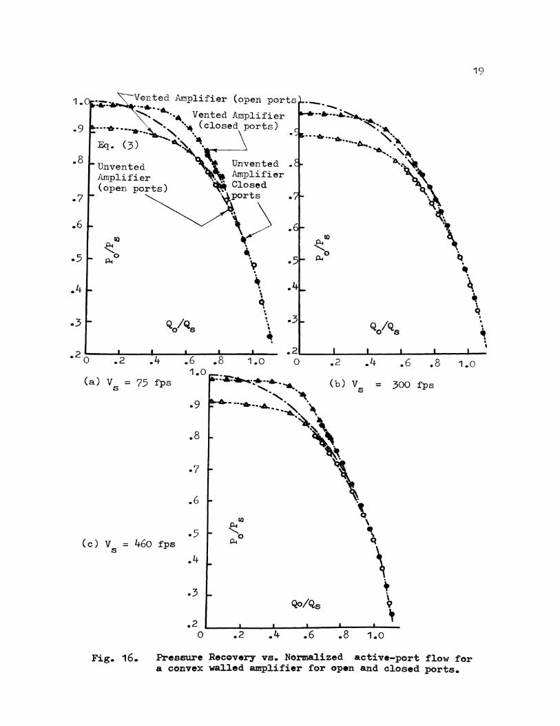
element unstable. This amplifier (Fig. 17) is capable of driving a

capacitive or reverse flowing load at high speed and with much smaller

control signals. The following points were kept in mind while designing

the amplifier configuration.

1. The receiver's reverse flow to be diverted away from the inter-

action region at the same time interaction region has to be

supplied with atmospheric pressure.

2. The receiver is required to develop satisfactory pressure and

flow recoveries during normal forward flowing operation.

The reverse flow from receivers escapes through vents v3 (Fig. 17).

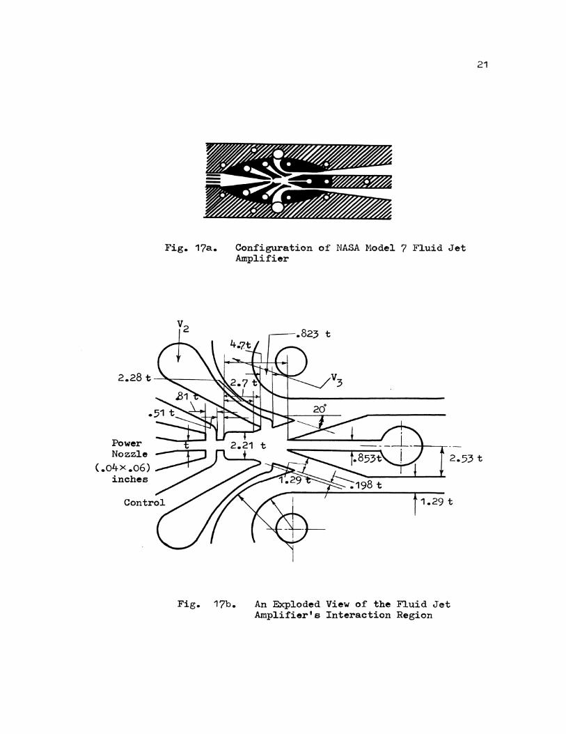
Fig. 17a. Configuration of NASA Model 7 Fluid Jet Amplifier

21

2.53 t

1.29 t

Fig. 17b. An Exploded View of the Fluid Jet Amplifier's Interaction Region

.1

0 0

Cenventional l Design j

I /,

0 Right-hand control port cLeft-hand control port

.20

Fig. 18.

.4o

--o--~ -.a---o--D

.60

P I P 0 s

.80 1.00

Contrel Pressures required to switch conventional and NASA Model 7 Fluid Jet Amplifier into reverse flowing receivers. Other receiver is vented to atmosphere.

22

23

A separate vent v2 provides the necessary entrainment flow. The baffle

between v2 and v3 prevents the reverse flow to disturb the interaction

region. It has been found that for a supply pressure of 1 psig, control

flow of only 10 - 15 % of the supply is sufficient to enable the

amplifier to drive a piston load under most conceivable modes of

operation. Figure 18 reveals that considerably less amount of control

pressure is necessary to switch the power jet into load receiver while

for a conventional amplifier switching pressure usual~ increases with

the load. The present design needs improvement in its manufacturing

techniques because its interaction region is sensitive to manu-

facturing errors.

Cascading Amplifiers:

It is essential to develop ana~sis techniques for cascaded

elements in fluidic circuits. Generally, the gains of individual

amplifiers are limited and a greater gain can be obtained through

cascading amplifiers. Belsterling [8] pointed out that input and

output characteristics of the elements to be cascaded are very

important considerations. The output characteristics demonstrate

the way in which the amplifier will behave with a load and the

input characteristics illustrate the switching flow requirements.

These two characteristics are superimposed (Fig. 19). As long as

the switching points of the input characteristics fall within the

boundaries of the output characteristics of the driving amplifier,

the elements are said to be roughly matched, however the cascading

operation will be more efficient when the switching points lie close

to the boundaries. In case they lie outside the output characteristics

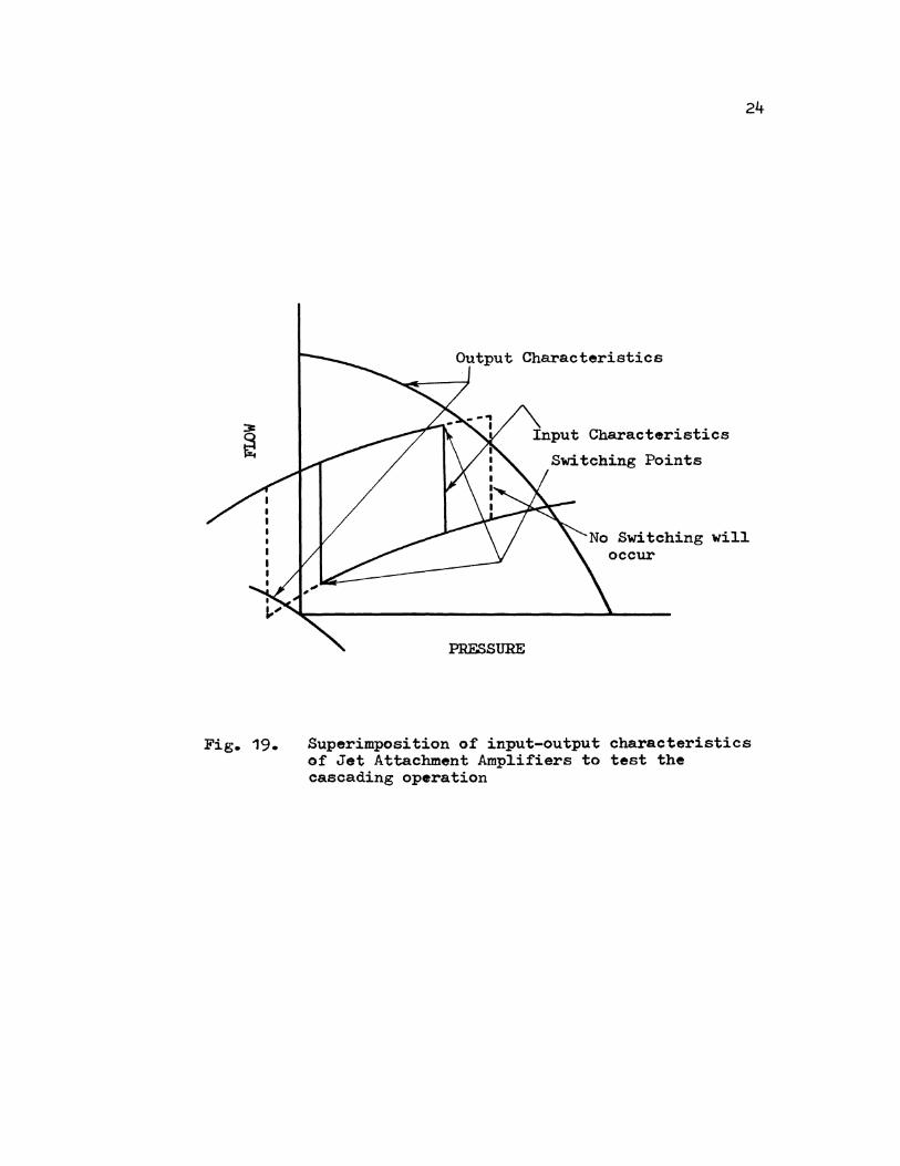
Fig. 19.

PRESSURE

Input Characteristics

Switching Points

24

No Switching will occur

Superimposition of input-output characteristics of Jet Attachment Amplifiers to test the cascading operation

25

of the driving element, the elements are not cascaded as the driven

element does not receive strong enough signals for switching. In

most digital circuits, an important requirement for the amplifiers

is to have high fan-out capability. It is defined as the number of

like elements an element can switch. A numerical analysis has been

included to find out the fan-out capability of a jet attachment

amplifier manufactured by Aviation Electric. Similarly the fan-in

capability is defined as the number of like elements that can switch

a given unit. It is desirable to bring all inputs directly into the

jet interaction region. However, due to physical limitations it is not

feasible to have .fan-in greater than 4, although a fan-in of 6 has

been reported.

To design a closed system (no vents) , each successive amplifier

has to be made bigger to accommodate the total flow coming from the

previous stage. An analysis by Hayes and Kwok [9] on latched vortex

vents (Fig. 20), located between two consecutive stages, does make

the cascading operation easier to some extent. In the normal operation

vent flow is negligible, with gradual blocking of output or even in

case of reversed flow to some extent, the flow escapes through the

vent without switching the main jet. In other words, as the output is

loaded, static pressure inside the chamber goes on increasing while

the vortex vent resistance goes on decreasing, thereby the flow

through the vortex vent increases. This element has a wide range of

operation along with the cascaded stages. It has appreciable pressure

recoveries but bas a draw back, that compression pulses propagate

back into amplifier's interaction region. The pressure and velocity

distribution flow equations for the outer annulus region as well as

Fig. 20.

~ Controls ---.. for

Second Stage

Sectional View at AA

Latched Vortex Vent Configuration as applied to a Fluid Amplifier

26

27

inner core flow region of the vent were derived in cylindrical co-

ordinates basically starting from the Navier-Stokes equations with

assumptions such as; the flow in the vent is steady, symmetrical

with respect to Z-axis, incompressible and it is fully established

and defined by the velocity vector in the annulus region r.<r (r • l. 0

Experimentally, a large scale model was under test that proved

the theory with water as the working fluid. Its flow pattern was

visualized and water velocities were determined from the length of

light streakes from the time exposure photographs of the water flow.

A Numerical Example for Cascading Amplifiers:

An Aviation Electric wall attachment amplifier (line matched),

has been used to test the normal staging of amplifiers and also to

find its fan-out capability. Refer to Figure 4 for its characteristics.

Following is some information for the amplifier;

Input pressure

Power consumption

Pressure Recovery (Blocked)

Flow Recovery (Open)

Frequency response

Response time

Switching flow

Switching pressure

Max.

15 psig

800 cps

Nominal

5.0 psig

4.1 watts

35%

125 %

0.0004 sec

0.110 scfm o.o6o scfm

1.15 psig 0.68 psig

Min.

2.0 psig

1.0 watt

0.035 scfm

0.31 psig

Assuming a supply pressure to the first amplifier to be 2.0 psig

for which switching flow is 0.035 scfm and switching pressure is 0.31

psig. Further assuming that supply press to the second stage is 5.0

28

psig which requires a switching £low o£ 0.60 sc£m and switching

pressure o.68~psig. It is observed from Figure 4 a. that the switching

requirement for the second stage cannot be met from the first stage

corresponding to a supply pressure of 2.0 psig since the switching

points lie outside the output characteristics of the first amplifier.

Increasing the supply to 5.0 psig would be more than enough. Since

the amplifiers have been equiped with vented vortex that can take

care of the extra pressure and flow to al1ow a successful cascading

operation.

T.he fan-out capability of the above mentioned amplifier can be

determined from the flow criterion. Corresponding to a supply of

5.0 psig and its switching pressure of 0.68 psig, the available flow

from the output characteristics (Fig. 4 a.) is found to be 0.22 scfm.

As the switching flow for a single element is 0.060 scfm, a fan-out

of 3 is suggested.

Total switching £low required £or three elements = o.o6)(3

= 0.18 scfm

The extra flow (0.22 - 0.18) scfm escapes through various vents

in the elements. Care bas to be taken since it is possible that the

vent flow may be larger than (0.22 - 0.18) scfm, in that case

a fan-out of only two is possible.

B. Turbulence Amplifiers

It is another kind of bistable amplifiers with no moving parts.

Basically it consists of two precisely aligned power tubes which have

been introduced into a vented cavity along with one or more control

29

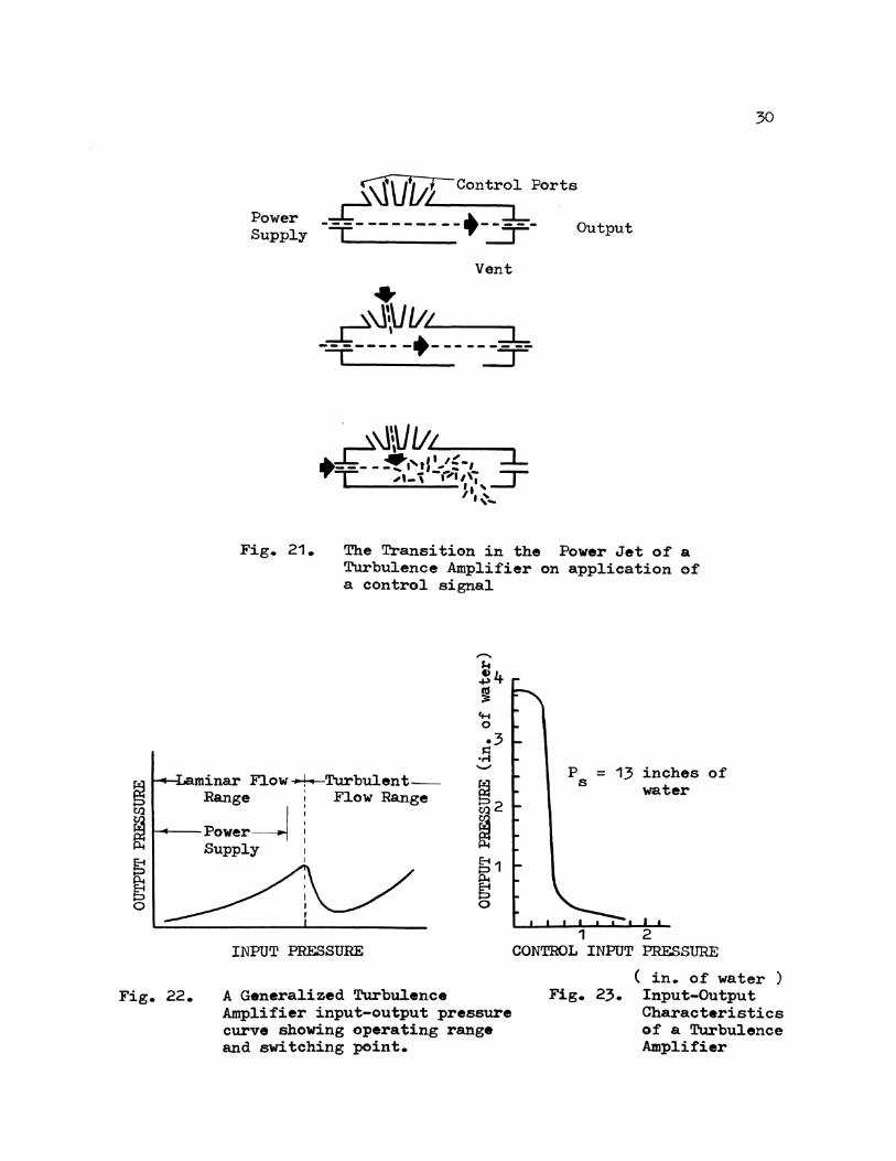
tubes placed across the main flow (Fig. 21).

In the absence of control signals, power stream is normally

laminar, consequently there is a high pressure recovery (Figs. 22-23).

As a control signal through any of the control tubes is applied, it

turns the main power jet turbulent. Since the spread rate of a turbu­

lent jet is greater than that of a lamjnar jet, a considerable

reduction in output pressure is noticed.

Turbulence Amplifiers have a very low power consumption. Output

pressure ranges from 2 inches of water (0.07 psi approx.) to less than

10 inches of water. T)pical flow rates vary from 1.5 to 3.0 cubic feet

per hour and Reynolds No. normal~ is 14oo. Sensitivity increases as

the Reynolds No. approaches the transition. As compared to other

fluidic active components such as a jet attachment amplifier or a jet

interaction amplifier, it has a very low power consumption because of;

1. Number of stages can be reduced because of high component

gain.

2. Power consumption per stage is less.

Turbulence amplifiers are relatively slow. The shortest practical

switching time is in the range of three milli-seconds. Improved

response is obtained through;

1. Increasing power flow or approaching transition, as a conse­

quence amplifier stability is sacrificed.

2. :s,. using strong signals i.e., overdriving the power jet.

Turbulence Amplifiers are relatively insensitive to mis-matches

with other circuit elements and have high fan-in and fan-out values.

In a report by Auger [1o], a fan-out approaching 20 is attainable by

modification of amplifier structure or by alteration of supp~

Power Suppl.y

Fi.g. 21.

r~Control. Ports

--;=- ------ --+-..:¥- Output

Vent

• ~\l~V LIL~___,. ..L-- ' - ::L --=e---- -·- -- --:::::r-

The Transition in the Power Jet of a Turbulence Amplifier on application of a control signal

30

~~m.inar F1ow~Turbu1ent---

~ Range FJ.ow Range

P = 13 inches of 5 water

ffi t----Power----1 Supply

I Fig. 22.

INPUT PRESSURE

A Generalized Turbulence Amplifier input-output pressure curve showing operating range and switching point.

1 2 CONTROL INPUT PRESSURE

( in. of water ) Fig. 23. Input-Output

Characteristics of a Turbulence Amplifier

31

pressure. Turbulence caused by control signals is also effected due

to geometrical parameters such as the diameters of input, output

and supply tubes, changes in the power jet velocity as well as

the viscosity and the density of the working fluid.

In another reference Auger [11] concluded that 0.030 inch for

the input-output tubes diameter satisfies the practical suitability

aspects such as power consumption, fabrication convenience, gain,

output volume and size of element etc. The input-output tubes are

kept 0.7 - 1.0 inches apart. I£ this distance exceeds 1.3 inches,

sound sensitivity begins. With increasing distance, the unit becomes

sensitive to high frequencies of the order of 10,000 cps. That is how

at a distance of 1.9 inches with a supply of 4 inches of water,

0.2 inches is recovered when the flow gets disturbed by a dog whistle

blown from a distance of 30 feet, but in case of no disturbance the

pressure recovered is 0.9 inches. On the other hand when this distance

is reduced below the range of high frequency sensitivity, it works

fine with approximate power gain from 4o to Bo. Decreasing the distance

further will result in reduced gain.

Following design hints for overall description of a Turbulence

Amplifier were given by Metzger and Lomas (12 J: 1. Nozzle Design;

a. To achieve a high gain the nozzle should be operated near

the critical Reynolds No. range (transition).

b. Unless sufficient length is allowed for the power nozzle,

laminar flow will not be achieved prior to power nozzle exit

and an earlier transition to turbulence is experienced.

32

2. Receiver Design;

a. Receiving aperture should have an area about the size of

the power nozzle.

b. As much open space as feasible must be allowed on all sides

of receiver to permit easy exit for the uncaptured flow.

c. Venting is essential as any resistance in the area reduces

the effective flow rate, reduces gain and increases power

consumption.

3. Control Nozzle Design;

Purpose of control nozzles is to deliver a turbulent flow

disturbance to the main flow, therefore,

a. Use very short length nozzles.

b. Allow the control jet to expand to spread rapidly to disturb

the main jet effectively.

In cascading turbulence amplifiers following characteristics need

be considered (Fig. 24).

a. Recovery pressure P vs. Control flow Q 0 c

b. Control flow Q vs. Control pressure P c c

c. Recovery pressure P0 vs. Recovery flow Q0

First the minimum control pressure and flow required to turn off

an amplifier are noted. Available flow from the output characteristics

of the driver element (P0 vs. Q0 ) corresponding to the switching

pressure of the driven element. Then the fan-out is determined by

dividing the available flow Q0 of the driver stage by the switching

flow Q of the driven stage. c

Numerically, 0.2 scfh is the control flow that can turn off the

output of an amplifier (Fig. 24 a.), control pressure is determined

(c) p 0

Fig. 24.

P (in. of \'later) output

(a) p vs. 0

33

Qcontrol

(scfh)

(b) p vs. Q c/ c ------

P ( in. of water ) c

Determining the Fan-out capability of a Turbulence Amplifier

34

from the curve P vs. Q (Fig. 24 b.) and is found to be 3 inches of c c

water. Using this pressure and referring to the curve P0 vs. Q0

(Fig. 24 c.) for a particular supply pressure (say 10 inches of

water), the available flow for driven elements is found to be

1.22 scfh.

Therefore, Fan-out = 1.22 0.2

~ 6

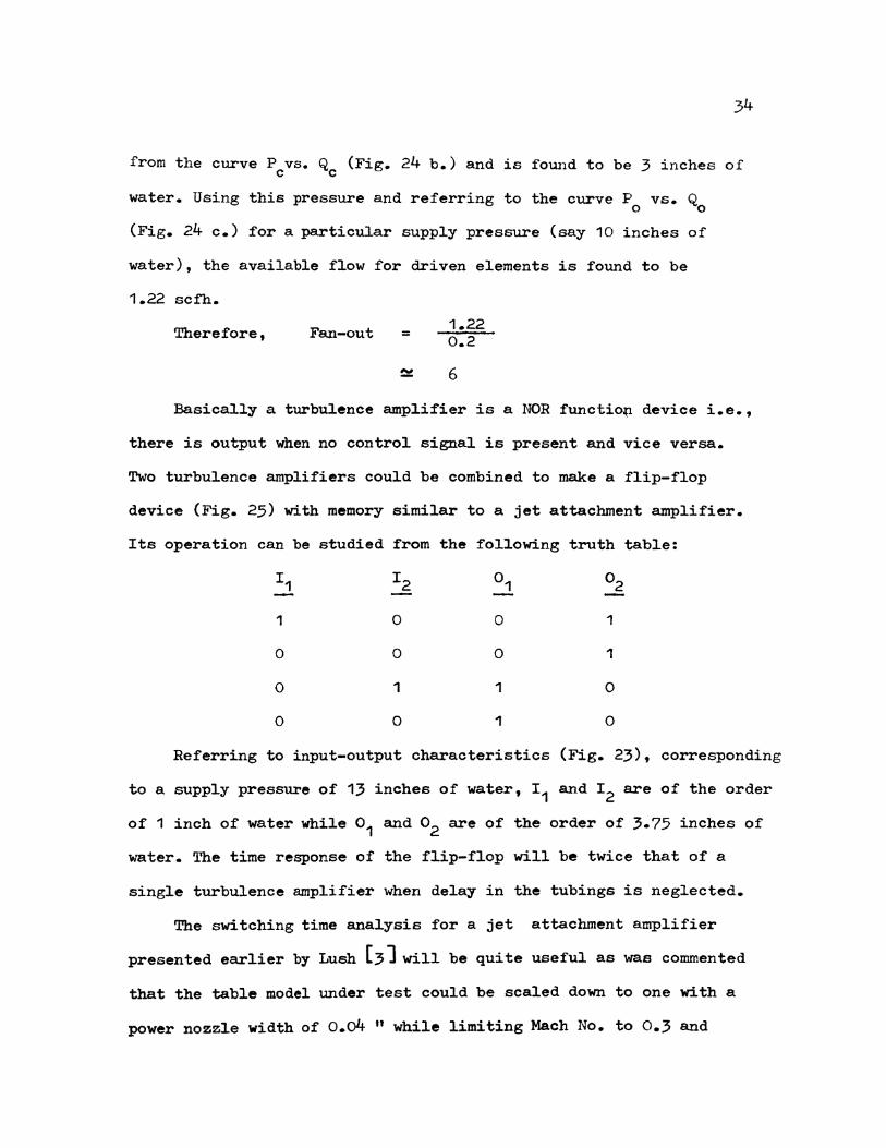
Basically a turbulence amplifier is a NOR functi~ device i.e.,

there is output when no control signal is present and vice versa.

Two turbulence amplifiers could be combined to make a flip-flop

device (Fig. 25) with memory similar to a jet attachment amplifier.

Its operation can be studied from the following truth table:

1 0 0 1

0 0 0 1

0 1 1 0

0 0 1 0

Referring to input-output characteristics (Fig. 23), corresponding

to a supply pressure of 13 inches of water, I 1 and I 2 are of the order

of 1 inch of water while o1 and o2 are of the order of 3.75 inches of

water. The time response of the flip-flop will be twice that of a

single turbulence amplifier when delay in the tubings is neglected.

The switching time analysis for a jet attachment amplifier

presented earlier by Lush [3] will be quite useful as was commented

that the table model under test could be scaled down to one with a

power nozzle width of o.o4 11 while limiting Mach No. to 0.3 and

Fig. 25.

J-4 J-4 • C) •r-1 •r-1 ft..t ct-t •r-1 •r-1 rl r-i

t ! • • 0 0 ~ ~ • • rl r-i

~ :;$

..0

~

r f

I 1

l 2

A Fluidic Flip-Flop Device Consisting of Turbulence Amplifiers

35

36

minimum Reynolds No. of 104 • Harda, Ozaki and Hara[5lused a

similar configuration but much smaller in size (0.02 " power nozzle

width), to optimize its various geometrical parameters such as vent

location, vent width and terminal crossing angle. Convex Coanda walls

(Fig. 15) were successfully shown by Sarpkaya (6] to be more efficient

as regards the pressure recovery which is described by equation (3).

An entirely new configuration (Fig. 17) by Griffin [7] is no doubt

more efficient, switching pressures do not increase with amplifier

loading, but the only problem lies in its manufacturing complications.

To illustrate cascading operation an Aviation Electric jet attachment

amplifier has been used to test the normal staging as well as to

determine its fan-out capability. For a successful cascading operation

either the driven elements have to be large enough to accommodate extra

flow or special Tents like latched vortex vents (Fig. 20) have to

designed. It can also be done through keeping the supply pressure for

the driver stages less than that for the driven stages.

37

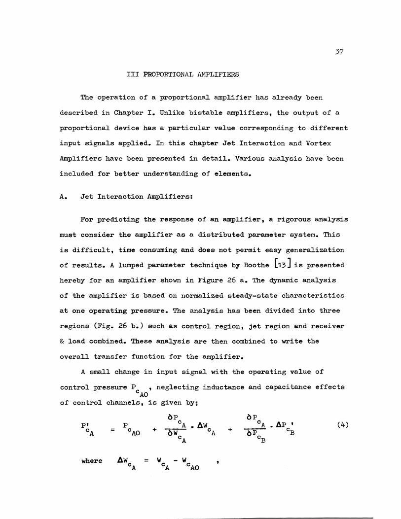
III PROPORTIONAL AMPLIFIERS

The operation of a proportional amplifier has already been

described in Chapter I. Unlike bistable amplifiers, the output of a

proportional device has a particular value corresponding to different

input signals applied. In this chapter Jet Interaction and Vortex

Amplifiers have been presented in detail. Various analysis have been

included for better understanding of elements.

A. Jet Interaction Amplifiers:

For predicting the response of an amplifier, a rigorous analysis

must consider the amplifier as a distributed parameter system. This

is difficult, time consuming and does not permit easy generalization

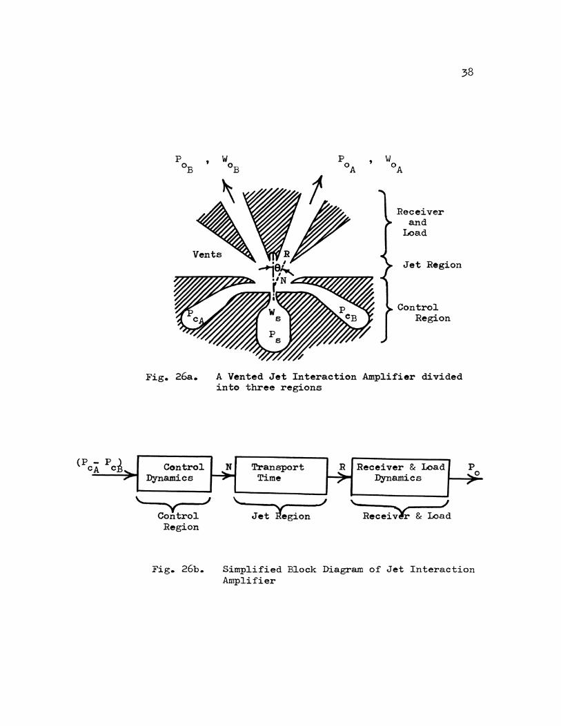
of results. A lumped parameter technique by Boothe [13] is presented

hereby for an amplifier shown in Figure 26 a. The dynamic analysis

of the amplifier is based on normalized steady-state characteristics

at one operating pressure. The analysis has been divided into three

regions (Fig. 26 b.) such as control region, jet region and receiver

& load combined. These analysis are then combined to write the

overall transfer function for the amplifier.

A small change in input signal with the operating value of

control pressure P , neglecting inductance and capacitance effects cAO

of control channels, is given by;

=

where =

+

- w .cAO

+ (4)

'

(P - p ) CA CB

\..

Fig. 26a.

Control. Dynamics

y Control.

.I

Region

Fig. 26b.

38

Receiver and

Load

Jet Region

Control. Region

A Vented Jet Interaction Amplifier divided into three regions

N Transport Time

\.... ~

Jet legion

R Receiver & Load Dynamics

\.. .I Recei~ & Load

p 0

Simplified BJ.ock Diagram of Jet Interaction Amplifier

39

4P I = p ' p ' - CA CA cAO

and 4P I = P' p cBO CB cB

Equation (4) is rewritten as,

4P 1 = K1;4w + K2 • 4P ' (5) CA CA CB

where .p

and l)P cA cA

K1 =.-w K2 = i"J> cA p = constant cB w = const.

cB cA

In above equations primed values show that the inductive and

capacitive effects have been neglected9 however accounted as follows;

Due to inductive effects there occurs some pressure drop in a

channel that accelerates the mass of fluid present in the channel.

or,

or,

Pressure drop = Passage Inductance • Mass rate of flow

(6)

where L = Equivalent inductance of the control passage c

Inductance of a passage is given by the following expression;

Inductance = Mass density • Length of path Effective cross sectional area of path

Similarly for the second control port B,

= L. s W c CB

(?)

Deflection of power jet at the nozzle exit is defined by the

the following equation;

(8)

where K3 is determined from receiver output characteristics.

4o

Equations (4) thru (8) could be combined to get,

G (AP -4P ) ~eN

c . = CA CB (1 + ~s)

(9)

where G =~ ( 1 + K2 ) c K1

.

and ~c' the control dynamics time constant = (1 + K2 )

Considering the transport time Tt from nozzle receiver,

( 10)

where~ is the deflection in power jet near the receiver.

Neglecting inductive effects, receiver pressure is related to the

jet deflection by the equation,

= (11)

Constants K4 and K5 are determined from the normalized receiver

characteristics.

Taking into account the inductive effects of the output channel,

(12)

where = Equivalent inductance of the output channel

Combining equations (11) and (12),

AP0 B = K4.~ - K5 [ 1 + <yx5).~ AW0 B (13)

Defining an operational impedence load

(14)

From equations (13) and (14),

= (15)

+ +

41

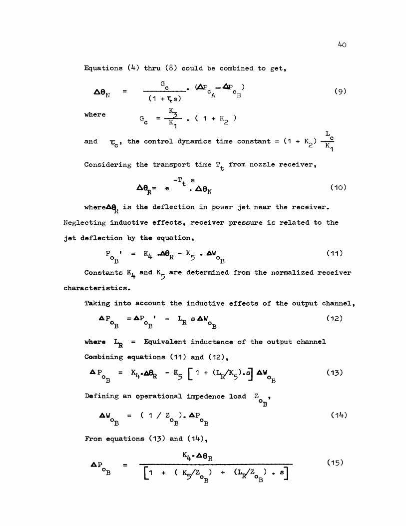
The overal1 transfer function is derived from equations (9),

(10) and (15);

-Tt s ( AP - AP ) G c • K4 • e c A cB

=(-1--+-~-c-.-s--)~[~1~+--(~K~5~;~z~o-B_) __ + __ (~~~~z-oB-)-.~~~---

(16)

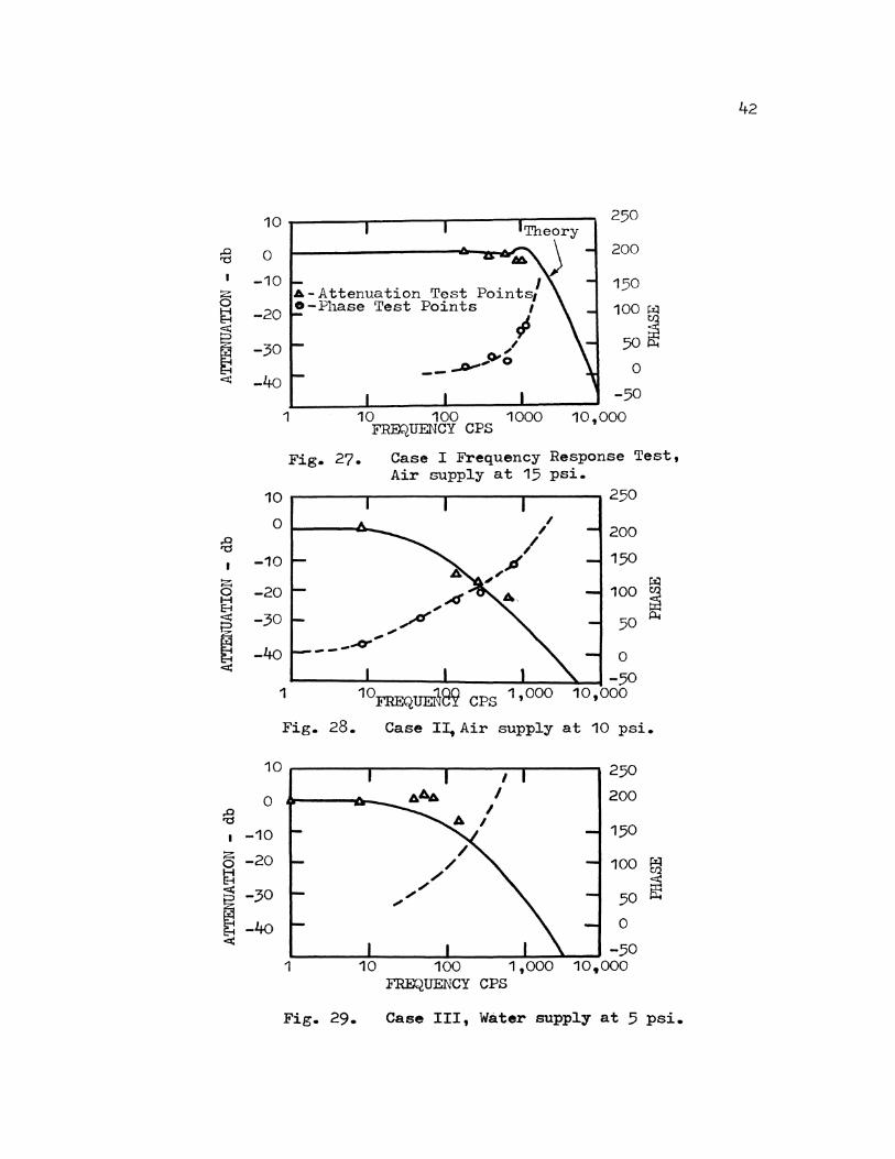
Frequency response data was taken in three sets. The first two

sets were obtained (Figs. 27 - 28) using air with supply pressures

15 and 10 psig respectively. Both the attenuation and the phase data

agree to the theory. In the second case there is a 5 cc vo1ume

dead ended load. Due to the vo1ume there is a first order break at

33 cps. Amplitude is in agreement with in 2.5 db. except for the

680 cps. point where exists a 4 db. discrepancy. In case III using

water with 5 psig supply on1y attenuation data was obtained (Fig. 29).

Analysis predicted a first order 1ag at 47 cps. Tests show peaking at

about 55 cps followed by a 20 db / decade drop off. The above test

results show that the norma1ized steady state data with a lumped

parameter approach is usefu1 and it gives more exact prediction for

air data with 1ow supp1y pressure.

Another technique by Be1sterling [14], that consists of equivalent

electrica1 circuits depending on the graphical characteristics. This

method predicts static and dynamic performance of a practical system.

Considering variables such as control differential pressure, control

differential flow9 amplifier pressure drop and amp1ifier output f1ow;

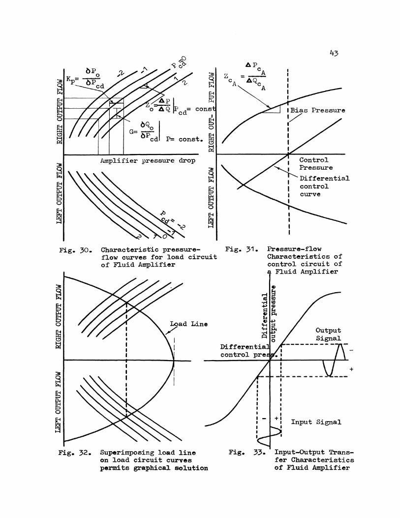
various plots appear in Figures 30-33 and they help describe the

e1ement.

The overa11 e1ectrica1 circuit of an amplifier is shown in

42

10 250 Theory

~ 0 200

I -10 .a.-Attenuation Test Points/ 150

:z; 0 o-Phase Test Points 1 100 ~ H -20 8 f 50~ I -30 /

" -- ~.,o,o 0 ~ -4o

-50 1 10 100 1000 10,000

FREQUENCY CPS

Fig. 27. Case I Frequency Response Test, Air supply at 15 psi.

10 250

0 I / 200

~ / I -10 ,.JI 150

~ "" ~ -20 Af 100 t:ll

8 /' ~ i§ -30 50

~ .,""

-40 ___ .... ~

0 ~

-50 1 1 0FREQUEI1ffi CPS 1,000 10,000

Fig. 28. Case II, Air supply at 10 psi.

10 250

0 200

~ I -10 150

:z; -20 /

0 / 100 ~ H / t:ll 8 ~ I -30

/ / 50 /

-4o 0 <(

-50 1 10 100 1,000 10.000

~UENCY CPS

Fig. 29. Case III, Water supply at 5 psi.

It---__,_---.~.,-..--

~

~p,

o =A Q P cd= cons

bQO I G= bPcd P= const.

I §

I Bias 1/ I I I I I

I

43

~Pressure

1 Differential 1 control 1 curve I

Fig. 30. Characteristic pressure- Fig. 31. Pressure-flow Characteristics of control circuit of a Fluid Amplifier

flow curves for load circuit of Fluid Amplifier

Line

Fig. 32. Superimposing load line on load circuit curves permits graphical solution

+

Output Signal

Input Signal

+

Fig. 33. Input-output Trans­fer Characteristics of Fluid Amplifier

44

Figure 34. This circuit has been simplified further for large

amplitude-high frequency signals and low amplitude-high frequency

signals (Figs. 35-36). In the first case a load line technique has

been used while for the second, parameters were linearized near the

operating point to evaluate the various electrical equivalent

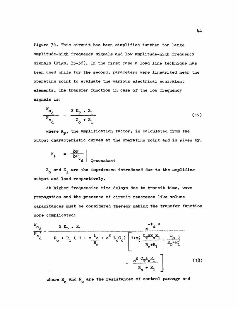
elements. The transfer fUnction in case of the low frequency

signals is;

= (17)

where ~' the amplification factor, is calculated from the

output characteristic curves at the operating point and is given by,

= Q=constant

Z0 and z1 are the impedences introduced due to the amplifier

output and load respectively.

At higher frequencies time delays due to transit time, wave

propagation and the presence of circuit reactance like volume

capacitances must be considered thereby making the transfer function

more complicated;

+

-t s e d

J where Rc and R0 are the resistances of control passage and

(18)

Fig. 35.

+ 1Qd

~--------P ' cd

Fig. 34. Complete electrical circuit equivalent for Jet Deflection Fluid Amplifier

Simplification for low frequency signals

Fig. 36. Simplication for high frequency signals

46

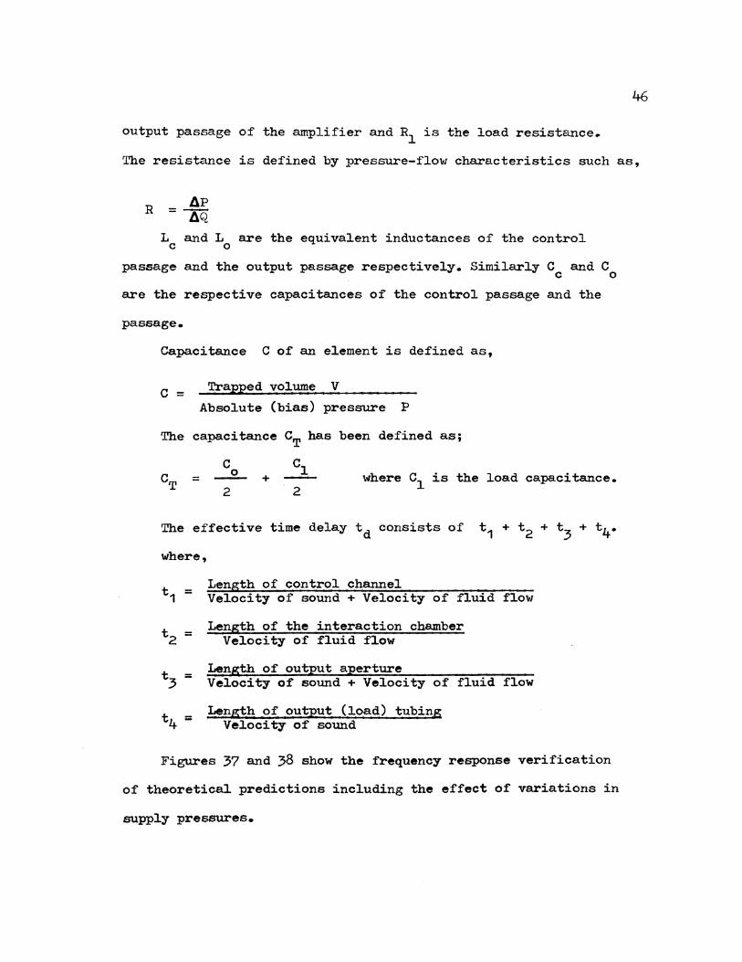
output passage of the amplifier and R1 is the load resistance.

The resistance is defined by pressure-flow characteristics such as,

R

L and L are the equivalent inductances of the control c 0

passage and the output passage respectively. Similarly C and C c 0

are the respective capacitances of the control passage and the

passage.

Capacitance C of an element is defined as,

c = Trapped volume V

Absolute (bias) pressure p

The capacitance CT has been defined as;

c = ---2.... where c1 is the load capacitance.

2

The effective time delay td consists of t 1 + t 2 + t 3 + t 4•

where,

Length of control channel Velocity of sound + Velocity of fluid flow

Length of the interaction chamber Velocity of fluid flow

Length of output aperture Velocity of sound + Velocity of fluid flow

Length of output (load) tubing Velocity of sound

Figures 37 and 38 show the frequency response verification

of theoretical predictions including the effect of variations in

supply pressures.

20

10

::§ I

z 0 0 H 8

~ -10

~ <

20

10

:§ 0 I

s -10 ~ ~ ~ <

1

1

---------o---.,.,. ---::...-.... ...... -- ... -_ ... !k

A- Calculated o -Experimental

5 10

FRJ!XtUENCY CPS

50

...... "'::o .... ~~ .... 0 ....

100

0

150

100

500

Fig. 37. Frequency Response of actual circuit with response calculated from equivalent circuit ..

100

0 -- --------~~~ -3 psig '"

,~,

50

5 10 50 100 500 FREQUENCY CPS

r4 til

r:a P..

Fig .. 38. Effect of variation in the Supply Pressure on Frequency Response of Fluid Amplifier

47

48

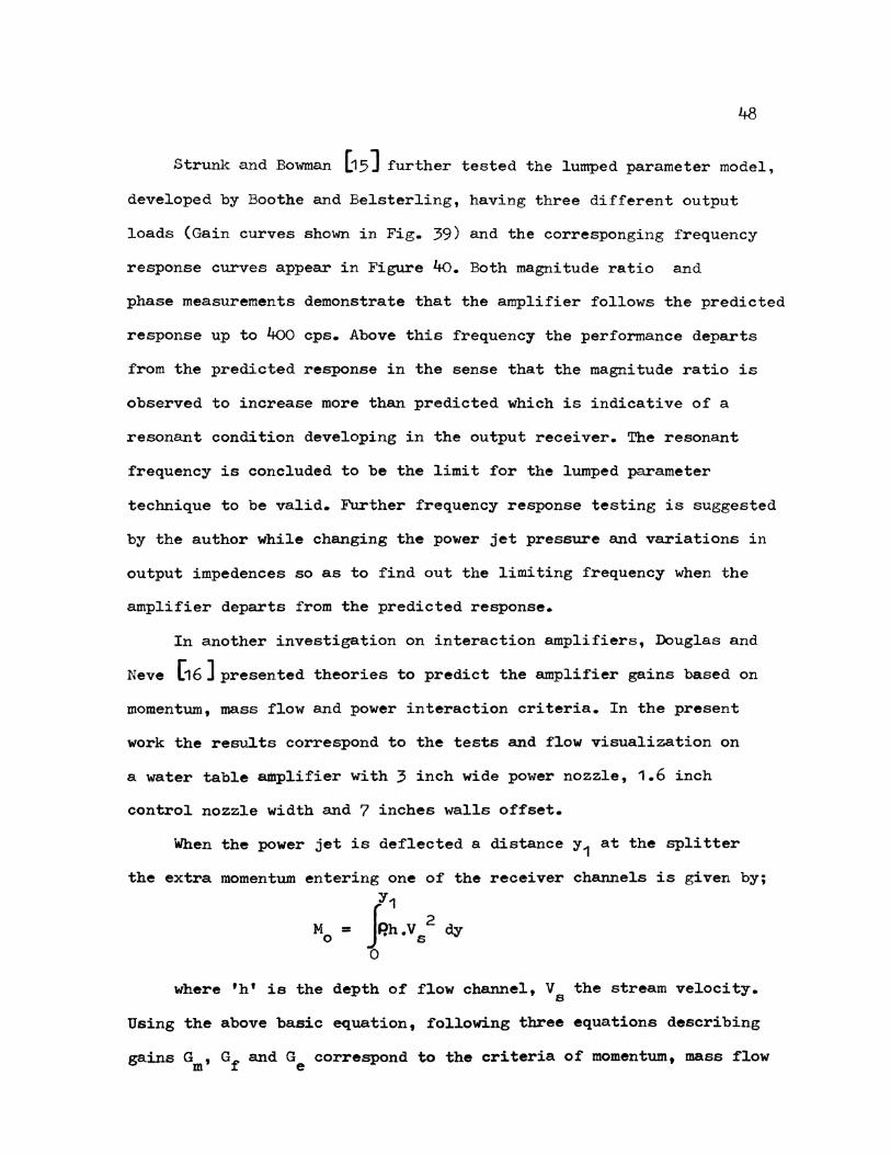
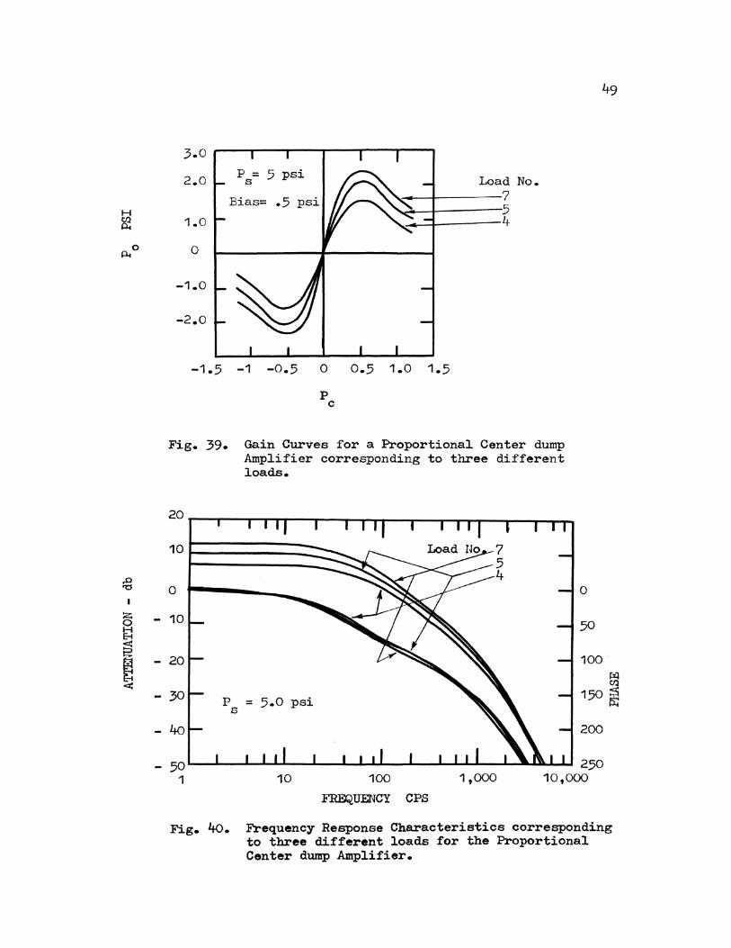
Strunk and Bowman [15] further tested the lumped parameter model,

developed by Boothe and Belsterling, having three different output

loads (Gain curves shown in Fig. 39) and the corresponging frequency

response curves appear in Figure 4o. Both magnitude ratio and

phase measurements demonstrate that the amplifier follows the predicted

response up to 4oo cps. Above this frequency the performance departs

from the predicted response in the sense that the magnitude ratio is

observed to increase more than predicted which is indicative of a

resonant condition developing in the output receiver. The resonant

frequency is concluded to be the limit for the lumped parameter

technique to be valid. Further frequency response testing is suggested

by the author while changing the power jet pressure and variations in

output impedances so as to find out the limiting frequency when the

amplifier departs from the predicted response.

In another investigation on interaction amplifiers, Douglas and

Neve [16] presented theories to predict the amplifier gains based on

momentum, mass flow and power interaction criteria. In the present

work the results correspond to the tests and flow visualization on

a water table amplifier with 3 inch wide power nozzle, 1.6 inch

control nozzle width and 7 inches walls offset.

When the power jet is deflected a distance y1 at the splitter

the extra momentum entering one of the receiver channels is given by; y1

M = rP.h • v 2 dy 0 J' s

0

where 'h' is the depth of flow channel, V the stream velocity. s

Using the above basic equation, following three equations describing

gains Gm' Gf and Ge correspond to the criteria of momentum, mass flow

H

ff 0

P-t

.0 '0

I

z 0 H 8

~ ~ <

3.0

2.0 p = 5 s psi

1.0

0

-1.0

-2.0

-1.5 -1 -0.5 0

p c

Load No. 7 5 4

0.5 1.0 1.5

Fig. 39. Gain Curves for a Proportional Center dump Amplifier corresponding to three different loads.

20

10

0

- 10

P = 5.0 psi s

0

50

100

200

- 50L-_.--~~~--L-~~~~-L--~~~~~LU~~ 250 10,000 1 10 100

~UENCY CPS

1 ,ooo

Fig. 4o. Frequency Response Characteristics corresponding to three different loads for the Proportional Center dump Amplifier.

and power interaction

G m =

1.08 c tan e

respectively.

I v: dy

0

Gf 1 + K y1

I o.451 :rt. = ij dy K s s

0

y1

G e /Xs k2

J 3

2.574 = v dy

K3 s

0

where V is the dimension1ess power jet ve1ocity, X is s

dimensionless downstream distance, X is splitter distance, y is s

50

(19)

(20)

(21)

dimensionless cross distance, K is the ratio of control mass f1ow

to power mass flow, k is the ratio of control nozzle width to

power nozzle width and C is an empirical constant.

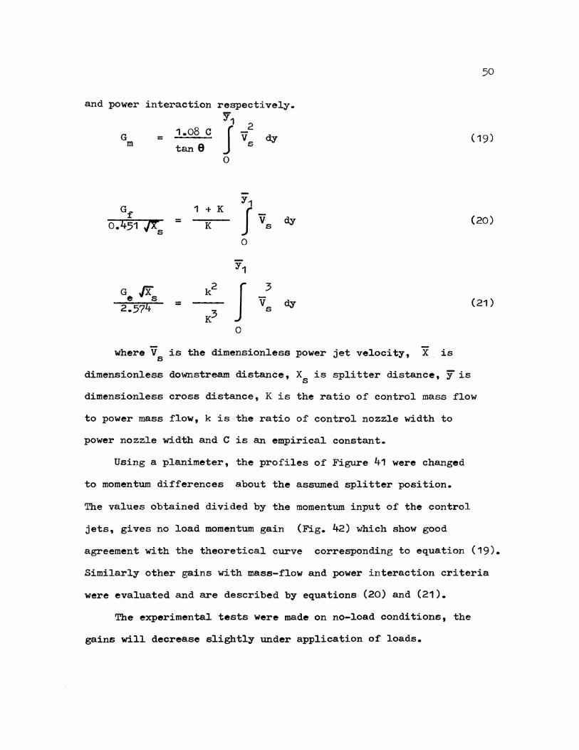
Using a planimeter, the profiles of Figure 41 were changed

to momentum differences about the assumed splitter position.

The va1ues obtained divided by the momentum input of the control

jets, gives no 1oad momentum gain (Fig. 42) which show good

agreement with the theoretical curve corresponding to equation (19).

Simi1ar1y other gains with mass-flow and power interaction criteria

were evaluated and are described by equations (20) and (21).

The experimental tests were made on no-1oad conditions, the

gains wi11 decrease s1ight1y under application of loads.

5

-; ...,4 ~

Ct-1 0

10 t) ~ 0 s:l3

·l"i -~ ~2 ~

~ A 1

Assumed Splitter Position

I I I I

11 12 13 14 READING ON TRAVELLING MICROSCOPE (em.) (Arbitrary Datum)

Fig. 41. Jet Profiles for Various Deflections

15

o K = 0 A 0.105 \ 0.146 v 0.173 7 0.225 "" o.28o

X = 17.3

R = 28,000 e

~ \J1 ~

z H :z;

c3 H

z :;31:

c3 H

t3 ~ ~ ~ til ~

E! ~ 6 ~

300 6

20

250 5

200 4 15

150 3 10

100 2

5

50 1

0 0 0 Momentum 0

Mass FlowO

Power 0 Gain

Fig. 42.

0

0

0

A I A A

Mass flow Gain

Momentum Gain

.05 .10 .15 .20

.05 .10 .15 .20

.02 .o4 .o6 .o8 .10

GAINS FUNCTION OF tan9

Comparison of' Theoretical and Experimental values of' Gains

52

tan9

tan9

tan9

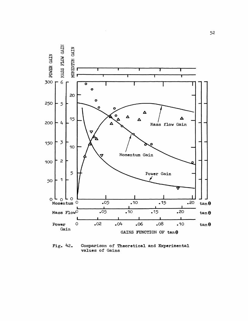
A unique configuration of a proportional amplifier (Fig. 43)

has been given by Griffin [17] similar to his analysis for a

bistable amplifier. Following are some of its improved features:

1. The maximum pressure gain obtainable for an ordinary

proportional amplifier is 7 compared to 11 for the

improved design (Fig. 44 a.).

53

2. The maximum normalized receiver output pressure was

found to be 52 % while for an ordinary amplifier it is

usually in the range of 4o - 50 % .

3. There is no drastic drop in output pressure in case of

strong signals. Configuration is such that the power

jet cannot be overdriven but in ordinary amplifiers

there is such problem present.

4. Three stages of new amplifiers are capable of giving

flat gain characteristics after saturation (Fig. 44 b.).

The zero shift encountered could be removed partially

by reducing aspect ratio and increasing supply pressure.

Constructionally, inclined ports are designed to limit power

jet deflection with the disadvantage that high gain with this kind

of amplifier should not be expected, although it is giving higher

value of gain than those conventionally available. There is a small

length of flat wall in the interaction region which does not let

the power jet attach when overdriven because of its short length.

A small offset of the interaction region's inclined walls serves

two purposes:

1. To dissipate small pressure waves generated by power

stream flow, that are peeled off by interaction region's

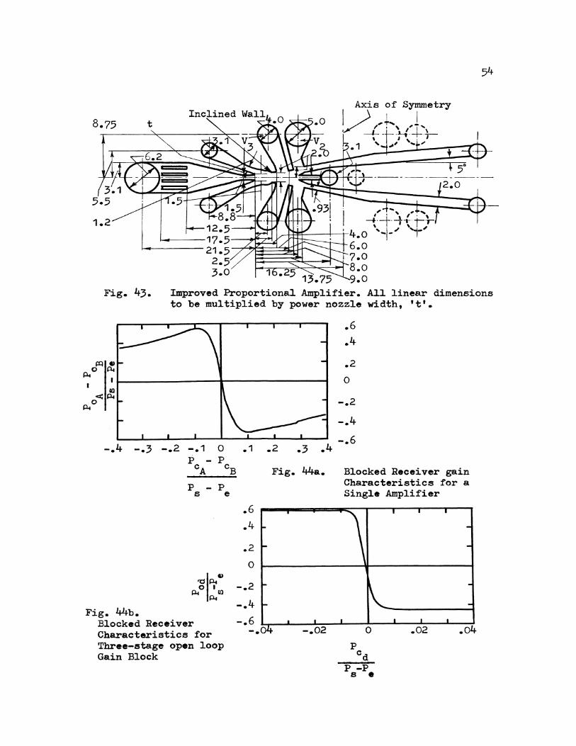
Fig. 43. Improved Proportional Amplifier. A11 linear dimensions to be multiplied by power nozzle width, 't' •

pq • 0 ~

~ ·~--------------~----------------i co

<~ ~0

-.4 -.3 -.2 -.1 0 .1

Fig. 44b.

p - p CA cB

p - p s e

Blocked Receiver Characteristics for Three-stage open loop Gain Block

.6

.4

.2

0

-.2

.2 .3 .4

Fig. 44a.

• 6 .4

.2

0

-.2

-.4 -.6

Blocked Receiver gain Characteristics for a Single Amplifier

p -P s •

.o4

55

exits.

2. It ref1ects the sma11 waves directly into the power stream

rather than letting it travel up to the contro1 port.

Cascading Amplifiers:

The gain of a sing1e amplifier is not high as required for an

operationa1 amplifier and so cascading is required to obtain the

necessary sain. Be1ster1ing GB] provided insight for the prob1em.

The design steps can be 1isted as fol1ows;

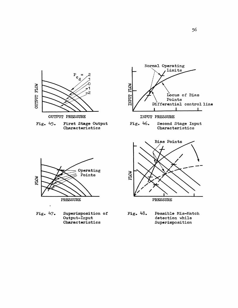
1. Obtain the output characteristics of the first stage

(Fig. 45). The curves (pressure vs. flow) are drawn

for different differential contro1 pressures.

2. Obtain the input characteristics of the second stage

amplifier (Fig. 46). These characteristics are of a

typica1 sma11 vented jet interaction amplifier with

0.010 X 0.025 inch power nozz1e width. Differential

contro1 curve is also shown (With a condition that

P + P = constant). This curve a1so indicates the CA cB

operating limits for the amplifier controls.

3. Superimpose the above characteristics on each other

(Fig. 47) which can tell exactly where the mismatch

lies and possibly a rectification.

Following are the classifications of mis-matches, which should

be checked one by one.

a. Matching operating bias points:

With superimposition of input-output characteri-

sties (Fig. 48), it is observed that the operating bias

OUTPUT PRESSURE

Fig. 45. First Stage Output Characteristice

Fig. 47.

PRESSURE

Superimposition of Output-Input Characteristics

Normal

\ . Locus of BJ.as Points

Differential control line

INPUT PRESSURE

Fig. 46.

Fig. 48.

Second Stage Input Characteristics

PRESSURE

Possible Mis-Natch detection while Superimposition

57

points do not match because the input characteristics

of the second amplifier is relatively steep. The possible

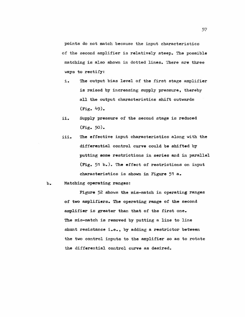
matching is also shown in dotted lines. There are three

ways to rectify:

i. The output bias level of the first stage amplifier

is raised by increasing supply pressure, thereby

all the output characteristics shift outwards

(Fig. 49).

ii. Supply pressure of the second stage is reduced

(Fig. 50).

iii. The effective input characteristics along with the

differential control curve could be shifted by

putting some restrictions in series and in parallel

(Fig. 51 b.). The effect of restrictions on input

characteristics is shown in Figure 51 a.

b. Matching operating ranges:

Figure 52 shows the mis-match in operating ranges

of two amplifiers. The operating range of the second

amplifier is greater than that of the first one.

The mis-match is removed by putting a line to line

shunt resistance i.e., by adding a restrictor between

the two control inputs to the amplifier so as to rotate

the differential control curve as desired.

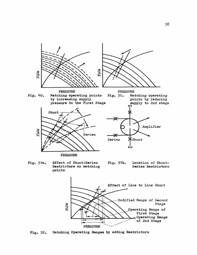
Fig. 49.

Fig. 51a.

Fig. 52.

PRESSURE Matching operating points by increasing supply pressure to the First Stage

PRESSURE

Effect of Shunt-Series Restrictors on matching points

PRESSURE Fig. 50. Matching operating

points by reducing supply to 2nd stage

m

Series

Fig. 51b.

)(

)(Shunt

L!.J

Location of Shunt­Series Restrictors

Effect of Line to Line Shunt

of Second Stage

perating Range of First Stage

~---H~;;~~~~~~~~~~~Operating Range of 2nd Stage

Matching Operating Ranges by adding Restrictors

Fluidic Operational Amplifier:

After it became feasible to cascade amplifiers, fluidic

operational amplifier came into existence. Doherty [19] presented

the basic approach in obtaining different functions such as;

59

integrating circuits, lead-lag or lag circuits along with the signal

summing operations.

An operational amplifier circuit (Fig. 53) consists of an

input resistor Ri' a feedback resistor Rf' a high gain five-stage

amplifier with a gain of -K (K = 2000 approx.) and an amplifier

control port resistance R • Flow at the summing junction is given c

by Kirchoff's

P.

p 0

l.

laws,

w1

- p g

R. l.

=

analogous

+ w2

+

-KP g

= p

where G = K

and

to current flow:

w3 (22)

- p p 0 g ....&.. = (23)

Rf R c

(24)

It is obvious from equation (26) that the transfer function is

determined from the values of Rf and Ri when G.H, the loop gain is

high.

R. P. - J.

J.

Fi.g. 53.

pb

FS-12 Summing Am l"f" P J. J.el"'

Control~ Output

Ap a

where K1

K2

K3

K4

K5

Fig. 54.

-

L!J

The Basic Fluidic Operational Amplifier

Flow Amplifier

1--- 1--

Bellows driven Hydro-mechanical

Actuator

K3 K4

p 0

K1 ~ (1 +T1 s) (1 +liS) wf Fuel Flow

=

=

= =

=

Fuel Metering

K5 Device

Position Transducer

45 psi/psi

1 psi/psi 0.03 "(1 = 3.8 Deg./psi 0.02 -r2 = 437 lb./Hr./Deg.

0.12 psi/Deg.

FS-12, Summing Amplifier in J-79 Turbo-jet engine control

sec.

sec.

60

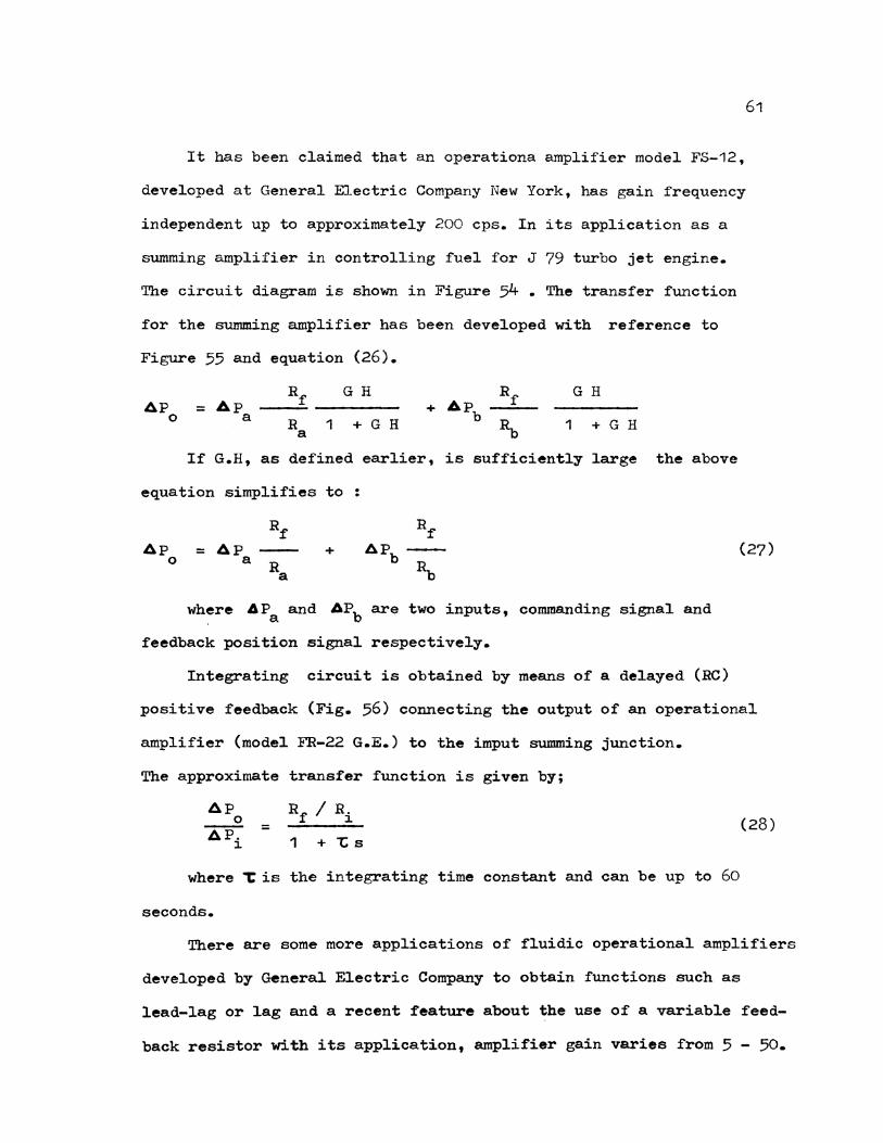
It has been claimed that an operationa amplifier model FS-12,

developed at General Electric Company New York, has gain frequency

independent up to approximately 200 cps. In its application as a

summing amplifier in controlling fuel for J 79 turbo jet engine.

The circuit diagram is shown in Figure 54 • The transfer function

for the summing amplifier has been developed with reference to

Figure 55 and equation (26).

AP 0

= Ap a

GH

1 + G H

G H

1 + G H

If G.H, as defined earlier, is sufficiently large the above

equation simplifies to :

61

Ap 0

= AP a + (27)

where 4Pa and APb are two inputs, commanding signal and

feedback position signal respectively.

Integrating circuit is obtained by means of a delayed (RC)

positive feedback (Fig. 56) connecting the output of an operational

amplifier (model FR-22 G.E.) to the imput summing junction.

The approximate transfer function is given by;

APO Rf I Ri

APi = 1 +"t:s (28)

where 1: is the integrating time constant and can be up to 60

seconds.

There are some more applications of fluidic operational amplifiers

developed by General Electric Company to obtain functions such as

lead-lag or lag and a recent feature about the use of a variable feed­

back resistor with its application, amplifier gain varies from 5 - 50.

I1

I2

a

Fig. 55. A Summing Amplifier's fluidic circuit

6P. J. --R.

J.

Fig. 56. An Integrating Fluidic Operational Amplifier Circuit

62

63

B. Vortex Amplifiers

The basic concept behind a vortex amplifier is of controlling

and amplifying a fluid flow by using a secondary flow. Supply flow

enters a cylinder and passed radially through a porous coupling

element into a vortex chamber (Fig. 57) and leaves this chamber

through an axial hole. Control flow enters tangentially into the

vortex chamber and as a consequence a vortex motion is set up that

restricts the output flow. This restriction is directly related to

the strength of the control pressure. There are two disadvantages

using a vortex amplifier:

1. The flow demand is hard to be reduced to zero.

2. Control pressure must be greater than the supply pressure,

thereby, too much power drain.

Letham [ 20] made analysis for the pressure distribution in the

vortex chamber, considering a differential fluid element radius rt

and radial thickness drt with tangential velocity Ut which is given

by the following equation:

2

p p P.uo

[ ( rt/ro )2 n 1] (29) = + r s 2 n

where p = Pressure at any radius rt in the vortex r

chamber

p = Supply pressure s

p = Mass density of fluid

uo = Tangential velocity inside the vortex chamber

rt = any radius in the vortex chamber

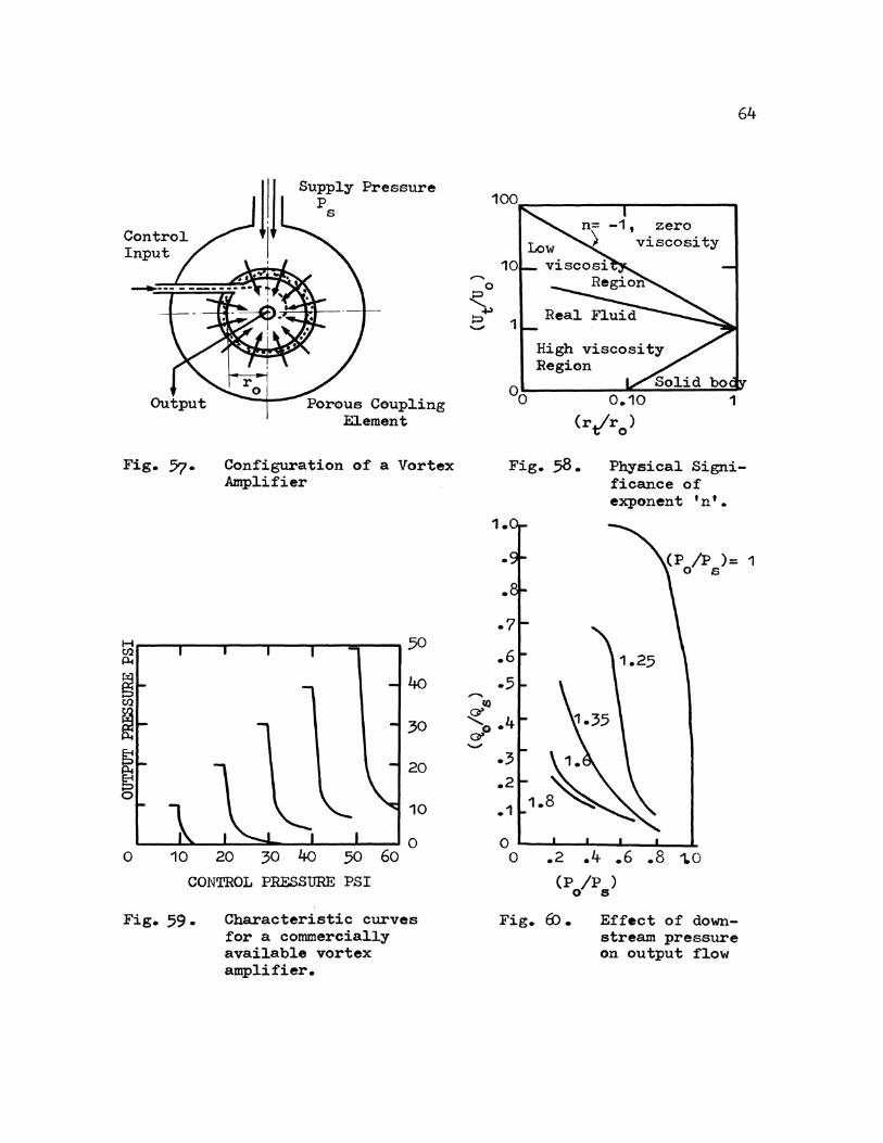
Control Input

Fig. 57·

Supply Pressure p

s

Porous Coupling Element

Configuration of a Vortex Amplifier

30

20

......... 1.0

Fig. 58.

• 6 .5

z 4 0. Of

.3

.2

64

n= -1, zero ) viscosity

Physical Signi­ficance of exponent 'n' •

10 .1

0 10 20 30 4o CONTROL PRESSURE PSI

Fig. 59. Characteristic curves for a commercially available vortex amplifier.

.2

(P /P ) 0 6

Fig. 8). Effect of down­stream pressure on output flow

r 0 = Maximum vortex chamber radius

· Ut' the tangential velocity at any radius is given by;

ut = uo.< r~ro )n

where 'n' is an exponent, its physical significance is given

in Figure 58.

(30)

The characteristic curves, for a commercially available vortex

amplifie~,., appear in Figure 59. It is observed that the output

pressure from the amplifier drops on application of the control

signal. The effect is similar to the one in Turbulence Amplifiers

but here the drop in pressure is more gradual as compared to the

abrupt drop in turbulence amplifiers, that is why they are made to

be used as digital devices and not proportional.

An unvented vortex amplifier is effected by the change in down­

stream pressure which is shown in Figure 60 by Larson [ 21] • Each

curve corresponds to a constant ratio of control pressure to supply

pressure. The curve with P /P ratio equal to one is for the case 0 s

when there is no vortex present in the vortex chamber. Venting of

amplifier is essential as the vent cavity provides a fixed static

pressure in the receiver, thereby isolating the vortex chamber from

downstream impedence changes.

Howland [22] introduced two configurations of vented vortex

amplifiers along with their characteristics (Figures 61-62) with

the difference that output receiving tube and the vent are located

on the same side in one case and opposite in the other. When the

vortex chamber is at full flow in the first geometry, the flow leaves

the exit hole as a solid jet and is so col1ected by the receiver.

Receiver

Fig. 61a.

Supply

Fig. 62a.

1 .8

......... 6 P-..,.4

.......... P..o.2

Fig. 62c.

Vortex Chamber

66

~~~~--~~~~,-~--r-~

45

4o

~35 Cll30

~25 E-t ~20 E-t

815 10

5

P = 100 psia s

Vent pressure = 15

Receiver outputs blocked

0 ~~--~-L--L--L~~~--~-J 100 120 CONTROL PRESSURE PSIA

A Vortex Amplifier Fig. 61b. Transfer Characteristics Receiver-Vent on same side

A Vortex Amplifier Receiver-Vent on opposite sides

100

~90 ~80 ~70 re6o

re~ g3o 20 10

0 0 90

Fig. 62b.

Effect of Vortex Geometry on Recovery Pressure

100

Transfer Characteristics

67

In the turn do~m condition it leaves in the form of a conical spray.

In the second configuration, the load flow is taken from a hole in

the opposite wall. The maximum dead ended pressure is close to the

supply pressure and the minimum is obtained at full control pressure.

Receiver pressure depends on parameters such as ambient pressure, Pe;

outside diameter d0 and vent diameter de. Figure 62 c. illustrates

how these effect the recovery pressure.

Vortex Amplifiers offer some unique applications for control

valves in modulating flow and powe~. They also find use in chemical

processing, natural gas control systems, engine fuel control, boiler

system control etc. A non-vented amplifier can be used in a flow

control system (Fig. 63). The flow sensor sendS a feedback signal into

the controller which appropriately sets the control signal to maintain

the output flow. The controller is made up of fluidic amplifiers and

performs the necessary summation, amplification anq/or integration

anq/or differentiation. Vented amplifiers are especially suited for

power amplification because they have the highest power recovery of

all fluidic amplifiers and they are not size limited. In an application

Larson [z1] presented a circuit with function of servo valve (Fig. 64).

In this circuit two vortex amplifiers are driven in push-pull by two

jet-interaction amplifiers. When there is no input signal,

=

=

If a control pressure P is applied, P and Q decrease while ~ ~ ~

p and Q increase. On application of P just the reverse happens. ~ ~ ~

This circuit differs from the conventional servo valves that the input

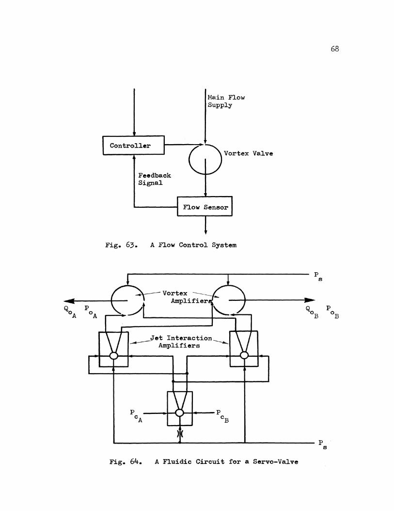
Main Flow Supply

Controller

Fig. 63.

Feedback Signal

Vortex Valve

Flow Sensor

A Flow Control System

Vortex Amplifier

Jet Interaction --- Am 1" f" ----...... p 1. 1.ers

)(

p B

~------------~------------_._______________ p

Fig. 64. A Fluidic Circuit for a Servo-Valve

68

B

signals are fluidic rather than electrical. Because of no moving

parts this fluidic servo valve has a high frequency response of

about 75 cps.

A lumped parameter approach by Boothe b3] and an equivalent

electrical circuit presented by Belsterling G4] to predict characteri­

stics of a jet interaction amplifier proved to be close. In a later

reference Strunk and Bowman [15] found this technique to be valid

until the resonance frequency of the output channel of the amplifier.

Douglas and Neve G6] predicted gain curves considering different

criteria for jet interaction such as momentum, mass flow and power

interaction. Griffin ~7] presented another efficient geometry for

jet interaction amplifier. cascading of amplifiers was explained

to achieve higher gains so as to make use to obtain an operational

amplifier. A fluidic operational amplifier does find its place in

integrating, lead-lag or lag circuits along with its use as a summing

amplifier. Vortex Amplifiers, which are basically proportional

amplifiers were explained their operation,:various characteristics

with typical performance data and their applications.

70

IV FLUID SENSORS

A sensor is an element which is sensitive to changes in operating

conditions such as temperature, pressure etc., and has an output that

varies with changes in operating conditions. Fluidic circuits

could be designed for various sensing operations. In this chapter

some fluid sensors have been presented and also their practical

design aspects have been studied. The Air Flow Velocity Sensor has

been included and its experimental analysis appears in the next

chapter.

A. Rotational Speed Measurement

There are two ways to measure rotational speed, using an

analog fluidic device (jet interaction amplifier) or a digital device

(Turbulence amplifier). In the analog device (Fig.65), the basic idea

is that of a pitot tube principle. As the angular velocity of disc

increases, air impinges on the openings in the disc edge thereby

increasing static pressure inside the tubing which links to one of the

control ports of an interaction amplifier. Thus, the pressure built

up in the receiver of the amplifier is the analog of rotational shaft

speed. Speed range for this device is limited by the disc diameter;

a larger diameter helps accummulate more static pressure that makes

the interaction amplifier reach its maximum gain (saturation) at an

early stage. Although saturation could be readjusted by changing the

biasing signal applied at the second control port of the amplifier

but it would also change the caliberation for the rotational speed of

shaft and the amplifier output. Response time of the sensor could be

improved by having a minimum tube length to carry the control signal

Fig. 65.

0

Fig. 66.

Fig. 67.

Receivers

Biasing Signal

Jet Interaction Ampli~ier

Rotational Speed Sensor using a Proportional Device.

Output Pulse

Rotational Speed Sensor using a Digital Device.

Output No. 1 ~ ~Supply

1

2

Output No. 2 ~

Torque Measuring Sensor

71

and also using a small sized proportional amplifier. Frequency

response of the amplifier is required to be good enough to handle

fluctuations in the shaft speed.

72

On the other hand the digital device setup (Fig. 66) is relatively

easier to build. Supply and receiver nozzles (turbulence amplifier)

are placed across a rotating disc, in the form of a gear or perfora­

tions in the disc, mounted on the shaft. In the output tube pulses

are formed that are counted and integrated with time to give the speed.

The frequency response of the digital pulse counting device limits

the maximum RPM that could be measured with this sensor. The square

pulse output is only an ideal case i.e., with increase in the rota­

tional speed, the pressure pulses in the receiving nozzle continue

getting flattened to the point when it is hard to count the pulses.

In other words the speed of the rotating disc is fast enough to make

a solid screen in front of the supply nozzle. Speed range could

further be increased to some extent by increasing pressure in the

supply nozzle. Frequency response of the pressure pulse counting

device essentially depends on the geometry of input-output nozzles,

supply pressure, distance between the nozzles (thickness of rotating

disc), and the diameter of the disc at the holes location, number of

holes in that diameter circle and geometry of the holes.

B. Torque Measurement

The arrangement is similar to the one used for the

rotational speed sensor with a digital device except, here two similar

discs (gears or discs with perforations) are mounted on a rotating

shaft, at a known distance apart (Fig. 67). This distance should be

73

less than the one producing a deflection equal to the angle between

two consecutive holes in the disc. The two pulse counters at the

two locations along the shaft tell a phase difference generated by

the relative angular displacement of the two ends, which is a

measure of torque when referred to the caliberation (phase difference

vs. torque). The design considerations for this sensor are the same

as for rotational speed sensor i.e., input-output nozzle diameter,

supply pressure, distance between the nozzles, diameter of disc at

holes location, number of holes in that diameter circle and hole

geometry.

c. Temperature Sensor and Control System

Atemperature sensing and control system developed by

Gottron and Gaylord [23] at H.D.L. consists of two similar fluidic

oscillators. These oscillators experience a change in frequency as a

result of the temperature change. The difference in frequencies from

the mixer, whose input links with the oscillators' output, is applied

to an acoustic to pneumatic converter (Fig. 68). The output from the

converter is operated upon by a digital logic circuit to yield a

pulse of constant amplitude and duration. These pulses are integrated

to obtain a 'd-e level' of flow or pressure that is a function of

difference in frequency of the two oscillators and hence the tempera-

ture. The output may be applied to a servo-valve, a hydraulic valve

or a reactor arm as per system requirement. Manual pre-set is the

bias control to the first stage of proportional amplifiers corres-

ponding to a pre-determined temperature maintenance. The fluidic

oscillator frequency is given by:

f = . ~ (V.R.T) I 4·1 (31)

,... ... ----- -... , Controlled

I I

I I I 1 Element I

L--r------J I I I I I t I I I ,-----------, I I I

Mixer

Osc. 1

Oac. 2

I I L --1 Controller t<--- Proportional

Amplifiers 1 I I I '-------- ---~

Manual Pre-Set

Accoustic to Pneumatic Converter

Digital Logic and Frequency to Analog

Conversion

Fig. 68. Proportional Temperature Control Syetem

1-

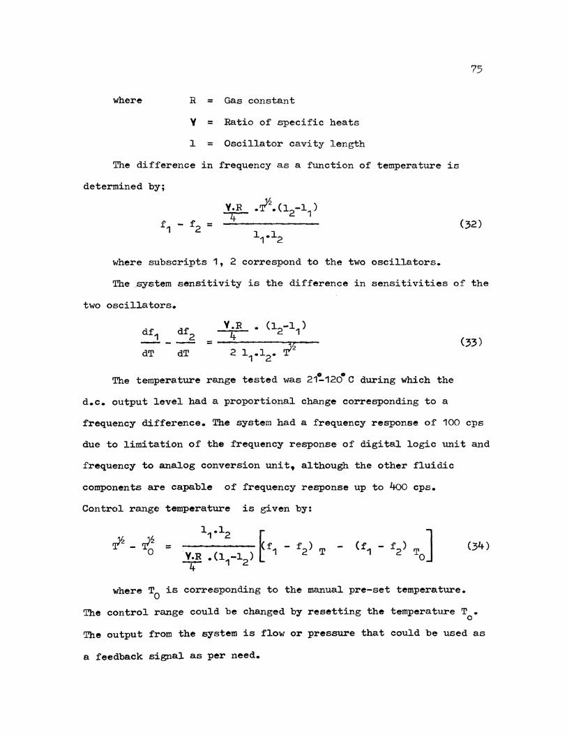
where R = Gas constant

V = Ratio of specific heats

l = Oscillator cavity length

The difference in frequency as a function of temperature is

determined by;

1;!- -~-(12-11)

11.12

where subscripts 1, 2 correspond to the two oscillators.

75

(32)

The _system sensitivity is the difference in sensitivities of the

two oscillators.

(33) dT dT

The temperature range tested was 21!.120• C during which the

d.c. output level had a proportional change corresponding to a

frequency difference. The system had a frequency response of 100 cps

due to limitation of the frequency response of digital logic unit and

frequency to analog conversion unit 9 although the other fluidic

components are capable of frequency response up to 4oo cps.

Control range temperature is given by:

(34)

where T0 is corresponding to the manual pre-set temperature.

The control range could be changed by resetting the temperature T • 0

The output from the system is flow or pressure that could be used as

a feedback signal as per need.

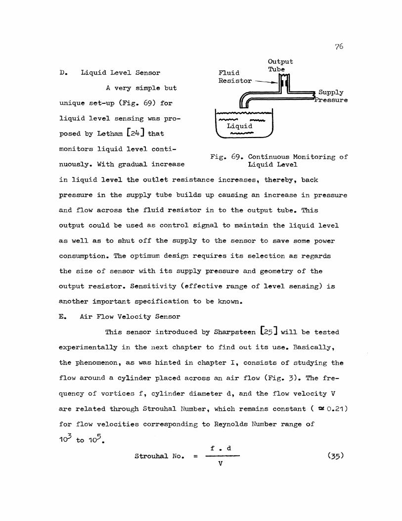
76

Output

D. Liquid Level Sensor Fluid Tube

A very simple but

unique set-up (Fig. 69) for

Resistor --IRI _ l!:-==::::=Jt Supply

dj(Pressure

liquid level sensing was pro-

posed by Letham [24] that

monitors liquid level conti-

nuously. With gradual increase

---Liquid

Fig. 69. Continuous Monitoring of Liquid Level

in liquid level the outlet resistance increases, thereby, back

pressure in the supply tube builds up causing an increase in pressure

and flow across the fluid resistor in to the output tube. This

output could be used as control signal to maintain the liquid level

as well as to shut off the supply to the sensor to save some power

consumption. The optimum design requires its selection as regards

the size of sensor with its supply pressure and geometry of the

output resistor. Sensitivity (effective range of level sensing) is

another important specification to be known.

E. Air Flow Velocity Sensor

This sensor introduced by Sharpsteen [25] will be tested

experimentally in the next chapter to find out its use. Basically,

the phenomenon, as was hinted in chapter I, consists of studying the

flow around a cy1inder placed across an air flow (Fig. 3). The fre-

quency of vortices f, cylinder diameter d, and the flow velocity V

are related through Strouhal Number, which remains constant ( a!0.21)

for flow velocities corresponding to Reynolds Number range of

1cY to 105. f • d

Strouhal No. = v

Knowing the frequency of vortices shed in the wake, the flow

velocity can easily be calculated. To measure the frequency,

77

a three-stage proportional amplifier will be used (although a bistable

amplifier can also be used with equal success) by connecting the

sensing holes drilled in the downstream side of the side of the

cylinder where the separation of flow occurs, to the control ports

of the amplifier. The amplified output will go to a transducer,

a charge amplifier and finally to an oscilloscope. Comments will be

made regarding the acuracy of this sensor as compared to the usual

use of a pitot-tube manometer. It will also be decided out of the

two tubes tested ( ~"and 1 "outside diameters ), which one is

better to use.

78

V AIR FLOW VELOCITY SENSOR

Basically the phenomenon used in the development of sensor is

the boundary layer separation and formation of Von Karman Vortex

Street in the wake of a cylinder placed across an air flow. When the

flow starts (low Reynolds Nos.) it is nearly frictionless. A fluid

particle in the thin boundary layer consumes much of its kinetic

energy on its path from D to E (Fig. 70) that it cannot climb the

pressure hill from E to F. The external pressure reverses the flow

which increases with the Reynolds No. A free vortex layer springs

from each separation point that establishes a circulation and

from which fluid in the form of vortices breaks away at regular

intervals.

Von Karman does not claim to have discovered these vortices.

Historically, the earliest picture in which he had seen them was in a

church in Bologna, Italy where St. Christopher is shown carrying child

Jesus across a flowing stream. Behind the saint's naked foot the paint­

er indicated alternating vortices. Von Karman contributed two fold

information. One that only the asymmetric arrangement of vortices

could be stable (Fig. 71), and only for a certain ratio of the distance

between the rows and the distance between two consecutive vortices

in either row. Also, he connected the momentum carried by the vortex

system with the drag, and showed how the creation of such a vortex

system can represent the mechanism of the wake drag.

Roshko [26) has shown data (Fig. 72) on cylinders with diameters

varying in the range of 0.00925 - 0.25 inches showing that the

phenomenon of vortex shedding is not dependent on diameter selection.

+

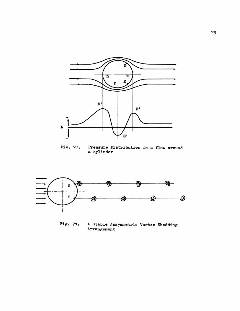
p t J

Fig. 70.

Fig. 71.

Pressure Distributi~n in a flow around a cylinder

A Stable Assymmetric Vortex Shedding Arrangement

79

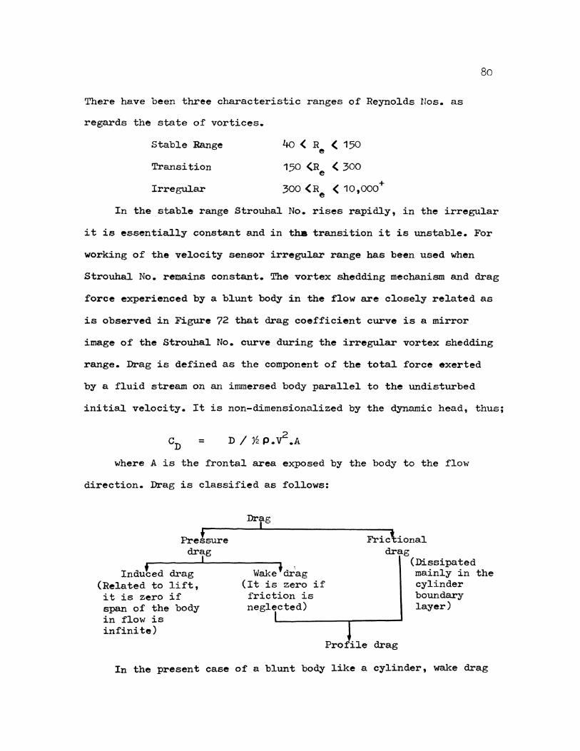
80

There have been three characteristic ranges of Reynolds Nos. as

regards the state of vortices.

Stable Range

Transition

Irregular

4o ( R ( 150 e

150 (R ( 300 e

300 (R ( 10,000+ e

In the stable range Strouhal No. rises rapidly, in the irregular

it is essentially constant and in tha transition it is unstable. For

working of the velocity sensor irregular range has been used when

Strouhal No. remains constant. The vortex shedding mechanism and drag

force experienced by a blunt body in the flow are closely related as

is observed in Figure 72 that drag coefficient curve is a mirror

image of the Strouhal No. curve during the irregular vortex shedding

range. Drag is defined as the component of the total force exerted

by a fluid stream on an immersed body parallel to the undisturbed

initial velocity. It is non-dimensionalized by the dynamic head, thus;

= D / ~ P.~.A

where A is the frontal area exposed by the body to the flow

direction. Drag is classified as follows:

Pre!sure drag

I

Induted drag (Related to lift, it is zero if span of the body in flow is infinite)

Waketm:ag (It is zero if friction is neglected)

Fric\ional drag

(Dissipated mainly in the cylinder boundary layer)

Pro ile drag

In the present case of a blunt body like a cylinder, wake drag

til

•

•22 " I I I I I I ' I I I :1 .. I I I I I ' ~ ~ ~ ·~ .;,... " r_l

.20

.18

',, Drag Coefficient B \ r "·'C- lf$:1:f..-IA,..t\~ '~~-l:_p --------~,---;t-t:.~--------__ : -- __ i'!.-

A ~-~# ~·~..AAI ·~o

a a ..,.<r' ~~\ ~

0 a <> 4

d = 0.00922 inches o.oaft25 8:8~1~

i .16 ·il t\i

• ~ • v

8·82~ o:1~5 0 250 I

til .14 ~

12 I I • I •I I I I

~t Data '6y Kovasznay Tails indicate that the velocity was computed from vortex frequency of a second cylinder.

I I I I

2.0

1.0

0

10 I I I I 1

20 4o 60 100 200 4oo 600 1 ,ooo 2,000 10,000

REYNOLDS NO. R • Fig. 72. Strouhal No. vs. Reynolds No. for circular cylinders

00 _,.

is dominating. It is also known as the Normal pressure drag. In

some more data by Wieselberger [27], CD the drag coefficient

has been measured for cylinders with diameter ranging 0.00197" to

11.8 11 (Fig. 73) and the Reynolds No. tested beyond 105•

It is seen near R = 5 X 105 , there is a sudden drop in the drag e

82

coefficient as a consequence of the transition in the boundary layer.

Transition causes the point of separation to move downstream which

considerably decreases the width of wake. In the plot pressure drag

coefficient and Strouhal No. vs. Reynolds No. (Fig. 72) following

points are observed:

1. CD' the drag coefficient is practically constant at

the value CD = 1.

2. The minimum point A is at a value of R close to that e

at which vortex shedding starts.

3. Maximum point B is in tha transition range.

4. In the irregular range CD is almost a mirror image of

the Strouhal No. curve.

Effect of Blunt Body Surface Roughness:

The influence of roughness enters into the problem of turbulent

skin friction. At low Reynolds No., it does not have a significant

effect on skin friction. The physical reason being that below this

limit the thickness of the laminar aublayer exceeds the height of

irregularities of the roughness elements which are not able to

produce additional turbulence in the main stream or in other words

the surface is said to be hydraulically smooth.

With increasing Reynolds No. the laminar sublayer becomes

thinner and thinner so that the roughness elements emerge and begin

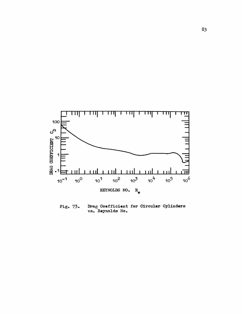
t:f~

~10 t)

5 1

8 t!:l

~ .1

10-1 10°

REYNOLDS NO. Re

Fig. 73. Drag Coefficient for Circular Cylinders vs. Reynolds No.

to influence the main flow. Now the skin friction is given by the

total frontal drag of these elements as every proturbance can be

considered as a small blunt body that contributes its individual

drag. The overall effect on the curve (Fig. 73) is to raise the

first part of the curve till R = 5 X 105 and the sudden drop in e

84

drag coefficient shifts to its left. This is because the transition

moves beyond the separation point in the upstream making the boundary

layer turbuJ.ent. As it is known that the turbulent boundary layer

sticks better to the surface, thus moving the separation point

further downstream. As result there is a narrow wake and hence a

drop in the drag.

This experimental set-up is capable of working in the Reynolds

No. range of 103 to 105 • Keeping into mind the dependence of Strouhal

No. on drag coefficient or in other words on the surface roughness,

it is advisible to specify the roughness of the tubes under test.

In the present work the tubes are assumed to be smooth.

Experimental Component Description:

Clear, cast lucite (acrylic) tubes of }!! " and 1 " outside

diameters were used with 1/16 " and 1/8 " respective wall thickness.

It is placed vertically in the middle of test section of the wind

tunnel. From top and bottom it is vented to downstream pressure. In

the middle of tube there was initially one hole ( 1/8 " diameter )

to sense the vortices. Later depending on the best signal detection,

• • the second hole was also dr1lled. The holes were found to be 115

downstream, close to the boundary layer separation point.

A G.E. 3-stage proportional amplifier model MG-11 was used to

amplify the pressure pulses due to the shedding of vortices. Three

custom designed proportional elements are cascaded in a close coupled

arrangement to minimize signal phase shift and excessive line

connections. Individual supply pressures are adjusted internally for

optimum performance. The manufacturer specified the following

characteristics:

Supply pressure

Maximum signal gain

Null bias

5 - 15 psig

100 : 1 (dead ended input)

negligible

Operating frequency 0 - 3,000 cps

Signal to noise ratio 100 : 1 below 25 cps

A quartz pressure transducer (KISTLER model 603 A) was used to

transduce the pressure signals to electrical signals. The transducer

contains an accelerometer positioned with in the pressure sensitive

quartz column to cancel out effectively spurious acceleration signals

over a wide frequency range. It measures very fast transients under

most environmental conditions. Response time is near micro-second.

KISTLER model 566 Multirange Charge Amplifier was connected

between the pressure transducer and the oscilloscope. This model

employs an electrometer tube input followed by a transistorized

voltage amplifier. Use of an electrometer tube in the input stage

makes the amplifier insensitive to accidental input overloads.

A stiff plastic tube of 1/8 11 I.D. and 1/4 11 O.D. was employed

for the supply flow to the fluid amplifier while for its input­

output connections a flexible tube of 1/16 11 I.D. and 1/8 " O.D. was

used. One output of the amplifier was blocked and the other connected

to the transducer. The length of input-output tubing is preferred to

be as short as possible to reduce the inductive and capacitive

effects present in a fluid line.

EA~erimental Procedure:

86

The two tubes ( 1/2 " O.D. and 1 " O.D. )used in the making

of the fluid sensor were tested in two sets of data each, corres­

ponding to single and double sensing holes.

First, the 1/2 " O.D. tube with single sensing hole was placed

in the flow (Fig. 74 a.) and rotated in order to get the best vortex

signal on the oscilloscope. This angular position of the sensing hole

(115° with the leading nose of the tube) was noted and subsequently

vortex frequency is noted. A pitot tube was placed in the centre of

the duct after removing the vortex sensor tube to determine the

corresponding velocities used for the velocity sensor. A second sensing

was then drilled in the tube corresponding to second separation point

(115° with the leading nose of the tube ) and all the above mentioned

steps were repeated. Next, the second tube ( 1 11 O.D. ) is similarly

tested for the same velocity range with single and double control

ports. Velocity in the wind tunnel varies from 25 fps to 75 fps in

five steps. Thus, five runs in each set make the total data consisting

of 20 runs which are repeated for pitot tube. Using above data,

Strouhal No will be evaluated separately for each run and th~from

the mean Strouhal No. value, the velocities of flow will be predicted.

Strouhal No. and Reynolds No. appearing in Table I were

evaluated corresponding to the experimental data ( Appendix A)

consisting of frequency measurements and the pitot tube velocities.

Strouhal No. will be evaluated using equation (~5).

Air Flow -

20 It

Wind Tunnel Vortex Sensor Tube Diffuser

Fig. 74a. Vortex Sensor Tube set-up in Wind Tunnel

Suction Fan

--. --.

00 ---.1

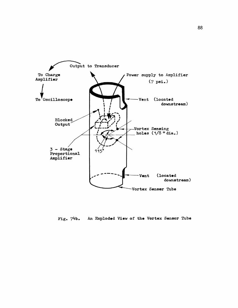
~ut to Transducer

To Charge Amplifier

To.Oscill.oscope

Blocked Output

3 - Stage Proportional Amplifier

supply to Amplifier

(7 psi.)

---Vent (located downstream)

{located downstream)

Sensor Tube

Fig. 74b. An Exploded View of the Vortex Sensor Tube

88

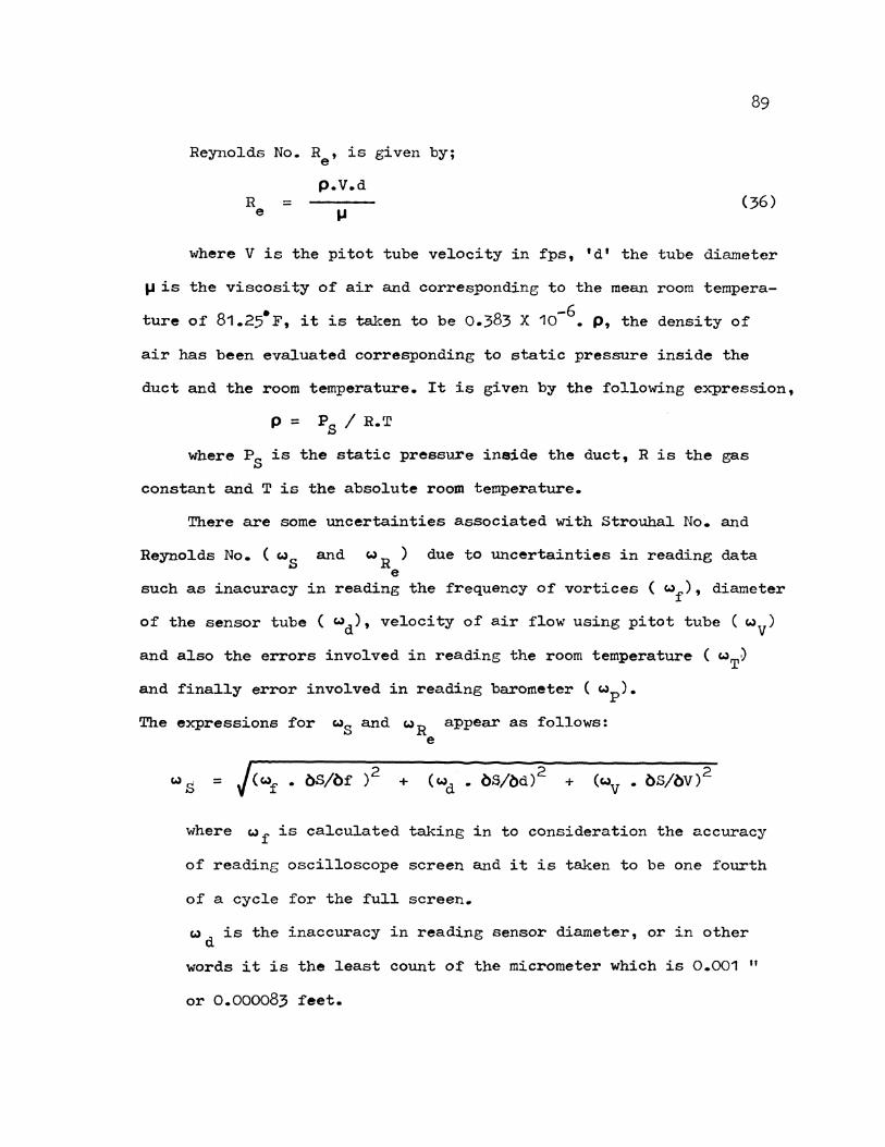
Reynolds No. R , is given by; e

89

R = e

p.V.d

.... (36)

where V is the pitot tube velocity in fps, 1 d 1 the tube diameter

1J is the viscosity of air and corresponding to the mean room tempera-

• 8 -6 ture of 81.25 F, it is taken to be 0.3 3 X 10 • p, the density of

air has been evaluated corresponding to static pressure inside the

duct and the room temperature. It is given by the following expression,

p = P8 I R.T

where P8 is the static pressure inside the duct, R is the gas

constant and T is the absolute room temperature.

There are some uncertainties associated with Strouhal No. and

Reynolds No. ( c,.)S and c.) R ) due to uncertainties in reading data e

such as inacuracy in reading the frequency of vortices ( c,.)f), diameter

of the sensor tube ( c.) d), velocity of air flow using pi tot tube ( c,.)V)

and also the errors involved in reading the room temperature ( c,.)T~

and finally error involved in reading barometer ( c,.)p)•

The expressions for c,.)S and c.) R appear as follows: e

= + +

where c.)f is calculated taking in to consideration the accuracy

of reading oscilloscope screen and it is taken to be one fourth

of a cycle for the full screen.

c,.)d is the inaccuracy in reading sensor diameter, or in other

words it is the least count of the micrometer which is 0.001 "

or 0.000083 feet.

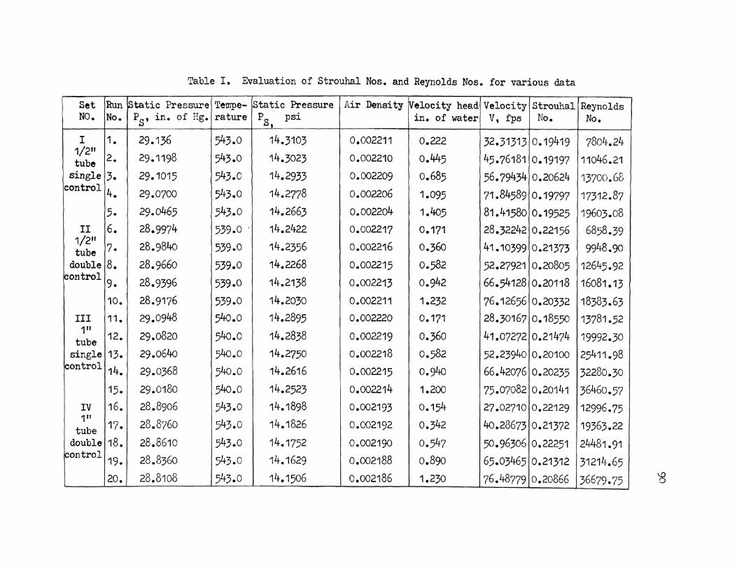
Table I. Evaluation of Strouhal Nos. and Reynolds Nos. for various data

Set Run Static Pressure Tempe- Static Pressure Air Density ~elocity head Velocity Strouhal Reynolds NO. No. P8, in. of Hg. rature Ps, psi in. of water V, fps No. No.

I 1. 29.136 543.0 14.3103 0.002211 0.222 32.31313 0.19419 7804.24 1/211

2. 29.1198 543.0 14.3023 0.002210 0.445 45.76181 0.19197 11046.21 tube single 3. 29.1015 543.0 14.2933 0.002209 0.685 56.79434 0.20624 13700.68

control 4. 29.0700 543.0 14.2778 0.002206 1.095 71.84589 0.19797 17312.87 .5. 29.046.5 .543.0 14.2663 0.002204 1.40.5 81.41.580 0.19.52.5 19603.08 I

II 6. 28.9974 539.0 . 14.2422 0.002217 0.171 28.32242 0.22156 6858.39 1/2" 7. 28.9840 539.0 14.2356 0.002216 0.36o 41.10399 0.21373 9948.90 tube

double 8. 28.9660 .539.0 14.2268 0.002215 0 • .582 52.27921 0.20805 12645.92 !control

9. 28.9396 539.0 14.2138 0.002213 0.942 66.54128 0.20118 16081.13 10. 28.9176 539.0 14.2030 0.002211 1.232 76.12656 0.20332 18383.63

III 11. 29.0948 54o.o 14.2895 0.002220 0.171 28.30167 0.185.50 13781.52 111

12. 29.0820 54o.o 14.2838 0.002219 0.360 41.07272 0.21474 19992.30 tube single 13. 29.0640 540.o 14.27.50 0.002218 0.582 52.23940 0.20100 2.5411.98

!control 14. 29.0368 540.o 14.2616 0.002215 0.940 66.42076 0.20235 32280.30 15. 29.0180 540.o 14.2523 0.002214 1.200 75.07082 0.20141 36460.57

IV 16. 28.8906 543.0 14.1898 0.002193 0.154 27.02710 0.22129 12996.75 1fl

17. 28.8760 543.0 14.1826 0.002192 0.342 40.28673 0.21372 19363.22 tube double 18. 28.8610 543.0 14.1752 0.002190 0.547 .50.96306 0.22251 24481.91

control 19. 28.836o 543.0 14.1629 0.002188 0.890 65.03465 0.21312 31214.65 20. 28.8108 543.0 14.1506 0.002186 1.230 76.48779 0.20866 36679.75 '8

wV is the inaccuracy in pitot tube velocity. The least count

for the inclined manometer (20° to horizontal) is 0.05 inch

or 0.0171 inch for a verticle scale. This inaccuracy is added

91

in the velocity head for each reading and the corresponding velocities

are calculated and hence the difference gives the uncertainty in the

pitot tube velcity.

= (~. bRe/ bV)2 +

-----------------

where wv and wd have already been explained. lUp is the least

count for the vernier scale mounted on the barometer equal to

0.002 inches of Hg. or 0.000983 psi.wT is the least count of the

thermometer and is equal to 0.5°F. w 5 and ~ appear in Table II. e

There were 20 runs in all to evaluate Strouhal No. and the

Reynolds No. range tested was from 7,000 to 37,000. A plot with

ordinates Strouhal No. vs. Reynolds No. appears in Figure 75.

In order to find the mean value of Strouhal No.,

Then

let fn (a) =A, the mean value of strouhal no., and let

f (x) is any data point on the plot. The subscript 'n' n

varies from 1 to 20, the number of runs.

f (x) - f (a) = deviation n n

1~e mean value for Strouhal No. will be obtained by minimizing

the function J.

J = 20

1 ~n (x) - fn (a)] 2

n=1

92

Table II. Percentage uncertainties in Strouhal Ntunber

and Reynolds Number

Run No. W_,. wv wn WR % w %w J. .::> s R e e

1. 5 1.12141 0.00930 270.941 4.79 3.47

2. 5 0.87067 0.00583 210.422 3.04 1.90

3. 5 0.7043 o.oo446 170.385 2.17 1.24

4. 5 0.5587 0.00328 135.608 1.66 0.78

5- 5 0.4941 0.00282 120.386 1.44 0.61

6. 5 1.38248 0.01304 334.836 5-89 4.88

7. 5 0.9648 0.00712 233-712 3.34 2.35

8. 5 0.76264 0.00500 184.863 2.4o 1.46

9. 5 0.60116 0.00362 146.076 1.80 0.91

10. 5 0.53671 0.00307 128.375 1.51 0.70

11. 1.25 1.38115 0.00970 676.960 5-23 4.91

12. 2.5 0.96383 0.00712 469.518 3.32 2.35

13. 2.5 0.76178 o.ooL~94 371.326 2.46 1.46

14. 5 0.60168 0.00653 293.959 3.23 0.91

15. 5 0.53268 0.00573 260.936 2.84 0.72

16. 1.25 1.46090 0.01248 702.619 5.64 5.40

17. 2.5 0.99460 0.00736 478.372 3.44 2.47

18. 2.5 0.79082 0.00501 380.576 2.25 1.55

19. 5 0.62232 0.00672 300.093 3-15 0.96

20. 5 0.53026 0.00563 256.550 2.70 0.70

.22

.21

• 20 ell ..

I .19

I ell .18

.17

I> ••

a a a

e

A

REYNOLOO NUMBER, R e

• • • ·Best fit curve for 1 "Tube: S= .2084

£est fit curve at S = 0.20589

Best fit curve for 1/2"Tube: S= .2033

E> 1/2 " Tube Single Control

(i 1/2 " Tube Double Control

A 1 tt Tube Single Control

.A 1 " Tube Double Control

Fig. 75. A Plot of Strouhal No. vs. Reynolds No. Corresponding to the the Experimental Data on the Vortex Sensor

~

or A =

=

20

n=1

20

f (x) n

4.11776

20 = 0.20589

The mean value of Strouhal No. is shown in the plot (Fig. 75)

94

along with mean values corresponding to 1/2 " and 1 " diameter tubes.

These are found to be o.2033 and 0.2084 respectively. For the sensor

velocity predictions these Strouhal No. values will be made use of

to find out which one of the two tubes gives close results.

Next a plot with variables pitot tube velocity vs. vortex

frequency is presented (Fig. 76) which is used to find fluctuations

in pitot tube velocity and the velocity obtained from the mean

slope of this plot and the available frequency data. The mean slope

K (assuming a linear functional relationship), is given by:

K =

The respective values of K for 1/2 11 and 1 " diameter tubes are

as follows;

~" = 1/4.815704

1/2.477748

The velocities obtained from this plot (Fig. 76) are assumed

to be more accurate than the pitot tube velocities (Table III)

since the mean slope of the plot deals in larger fluctuations to

smooth out than the uncertainty present in the pitot tube velocities.

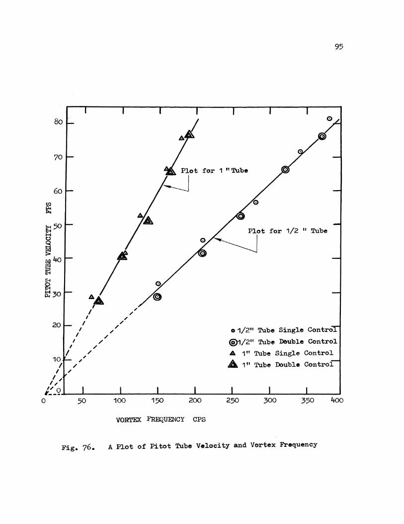
20

I I

I

I I

I

I 4,. I

I

50 100 150 200

95

for 1 "Tube

e 1/2" Tube Single Control

@1/211 Tube Dcuble Control

A 1 11 Tube Single Control

A 1 11 Tube Double Control

250 300 350 4oo

VORTEX :F'R&tUENCY CPS

Fig. 76. A Plot of Pitot Tube Velocity and Vortex Frequency

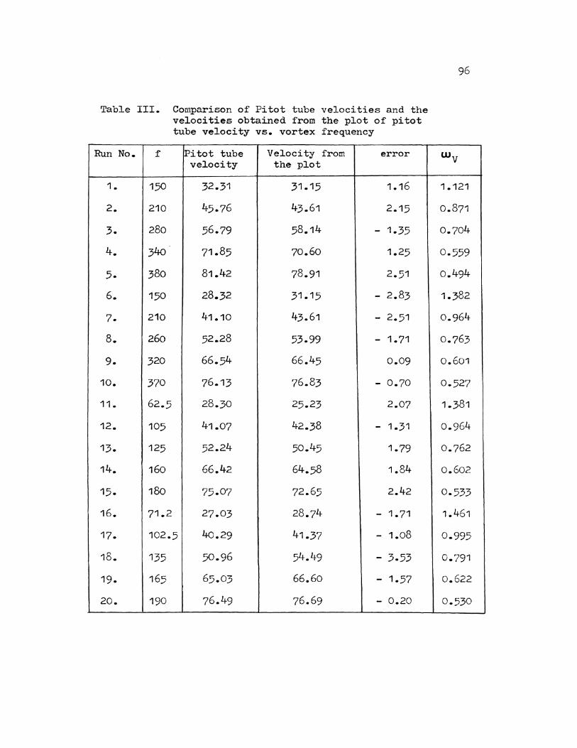
Table III. Comparison of Pitot tube velocities and the velocities obtained from the plot of pitot tube velocity vs. vortex frequency

Run No. f Pitot tube Velocity from error velocity the plot

1. 150 32.31 31.15 1.16

2. 210 45.76 43.61 2.15

3. 280 56.79 58.14 - 1.35

4. 34o 71.85 70.60 1.25

5- 380 81.42 78.91 2.51

6. 150 28.32 31.15 - 2.83

7. 210 41.10 43.61 - 2.51

8. 260 52.28 53.99 - 1.71

9. 320 66.54 66.45 0.09

10. 370 76.13 76.83 - 0.70

11. 62.5 28.30 25.23 2.07

12. 105 41.07 42.38 - 1.31

13. 125 52.24 50.45 1.79

14. 160 66.42 64.58 1.84

15. 180 75.07 72.65 2.42

16. 71.2 27.03 28.74 - 1.71

17. 102.5 4o.29 41.37 - 1.08

18. 135 50.96 54.49 - 3-53

19. 165 65.03 66.60 - 1.57

20. 190 76.49 76.69 - 0.20

96

wv

1.121

0.871

0.704

0.559

0.494

1.382

0.964

0.763

0.601

0.527

1.381

0.964

0.762

0.602

0.533

1.461

0.995

0.791

0.622

0.530

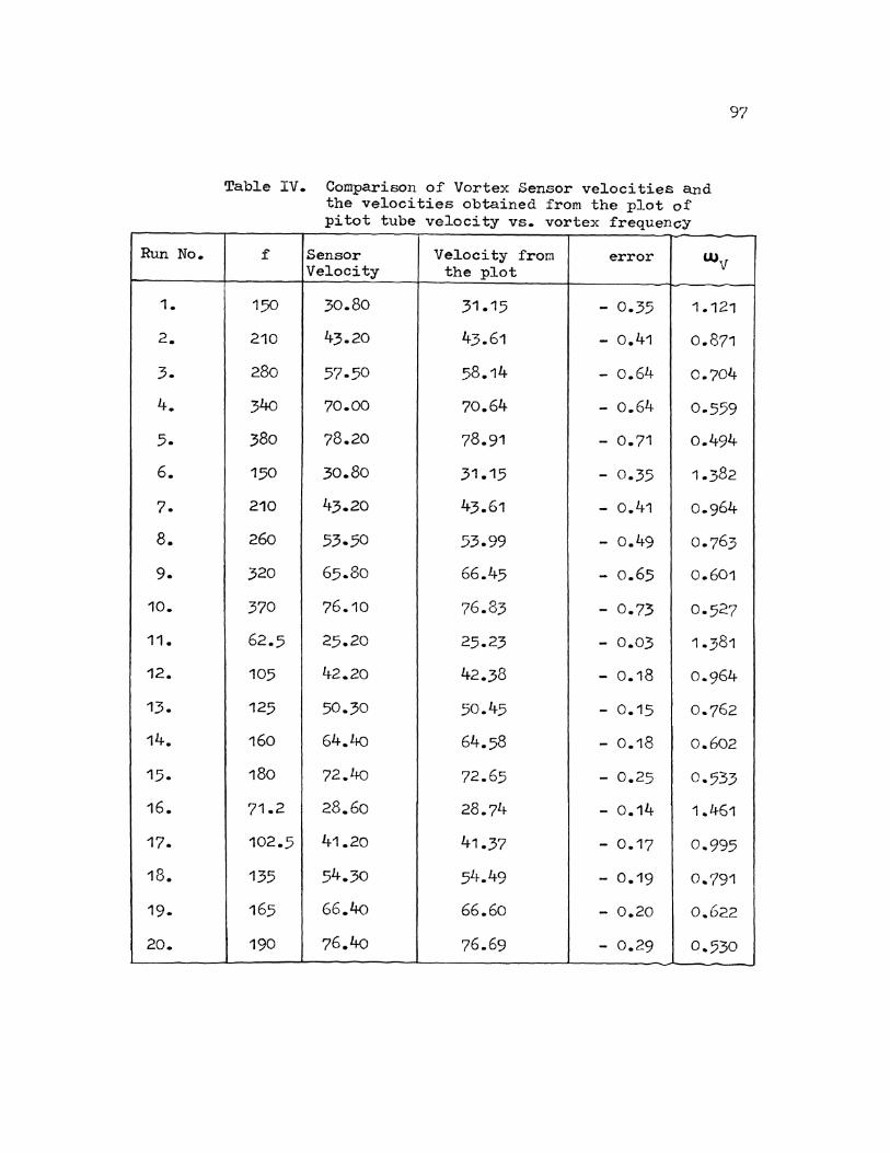
Run No.

1.

2.

3.

4.

s. 6.

7.

8.

9.

10.

11.

12.

13.

14.

15.

16.

17.

18.

19.

20.

97

Table IV. Comparison of Vortex Sensor velocities and the velocities obtained from the plot of pitot tube velocity vs. vortex frequency

f Sensor Velocity from error UJV Velocity the plot

150 30.80 31.15 - 0.35 1.121

210 43.20 43.61 - 0.41 0.871

280 57-50 58.14 - 0.64 0.704

34o 70.00 70.64 - 0.64 0.559

380 78.20 78.91 - 0.71 0.494

150 30.80 31.15 - 0.35 1.382

210 43.20 43.61 - 0.41 0.964

260 53-50 53.99 - 0.49 0.763

320 65.80 66.45 - 0.65 0.601

370 76.10 76.83 - 0.73 0.527

62.5 25.20 25.23 - 0.03 1.381

105 42.20 42.38 - 0.18 0.964

125 50.30 50.45 - 0.15 0.762

160 64.4o 64.58 - 0.18 0.602

180 72.4o 72.65 - 0.25 0._533

71.2 28.60 28.74 - 0.14 1.461

102.5 41.20 41.37 - 0.17 0.995

135 54.30 54.49 - 0.19 0.791

165 66.4o 66.60 - 0.20 0.622

190 76.4o 76.69 - 0.29 0.530

These velocities will then be used as reference for the sensor

velocities. The sensor velocities are calculated by the Strouhal

Number expression already described. The exact diameters of the

two tubes are 0.502 11 and 1.008 "· Thus the sensor velocities are

compared with the respective velocities evaluated from the mean

slope of the plot of pitot tube velocity vs. frequency of vortices

shed (Table IV). The errors obtained using the sensor are considerably

less than the uncertainty in the pitot tube velocities. Further it

is observed that the errors for 1 n diameter tube are smaller as

compared to the 1/2 " diameter tube.

Comments as regards the Velocity Range of Vortex Sensor and its tube

diameters:

The feasibility of the velocity sensor was due to the fact that

Strouhal No. remains constant in the Reynolds No. range of 103 to 105•

Corresponding to this range 1/2 " diameter sensor tube could be

operated in the velocity range of 4.04 fps to 4o4 fps v1hile for 1 11

tube it is 2.02 - 202 fps. Due to the limited velocity range

available from the wind tunnel ( 25 -75 fps approx.), the sensor

could be tested for the Reynolds No. range of 7,800 to 19,600 in case

of 1/2 " tube and 13,000 to 36,700 for 111 tube. The h1o Reynolds No.

ranges tested are although different but have an overlap from 13,000

to 19,600.

The Strouhal No. evaluations indicate consistent values irrespec­

tive of the tube diameters, ho\·lever, separate mean Strouhal No. values

were used to deter~ine the individual performance of the tubes.

1 " tube proved to be better due to following points.

Large diameter tubes are useful for low velocities. Observing

the Reynolds l'Jo. range, 1 11 tube could probe lower velocities as

compal'ed with 1/2 11 tube for the same Reynolds No.

99

A pi tot tube-manometer set has increasing uncertainty as l01.1er

velocities are approached due to inaccuracy in reading manometer.

For a flow velocity of 25 fps there has been found to be an error

of 1.5 fps which further increases with lower velocities. It is

recommended to use a vortex sensor in the range from 25 fps to

further lower velocities. Although the 1/2 11 tube is supposed to

have a greater sensitivity i.e., larger~f for the same~V (Fig. 76),

still 1 " tube was found to have smaller errors associated than

those with 1/2 " tube. The smaller tubes are limited by the

frequency response of the fluidic circuit due to higher frequency

of vortex shedding. A fevJ more tubes with larger diameter (say 1}'2 11

or 2 " or may be 3 " too) are suggested to be tested to decide

upon a particular tube for a certain velocity range.

VI SUMMARY AND CONCLUSIONS

A study of the Air Velocity Sensor, using a three staged

proportional amplifier to sense the vortices shed in the wake of

a cylinder placed in a flow, indicates that it gives a precise

measurement of velocity. Two different(1/2 " and 1 ") diameter

tubes were used. It has been concluded in the previous chapter

100

that 1 " diameter tube is better as for as acuracy is concerned and

also more effective for low velocities. The usual way to measure

velocity of air through the use of a pitot tube, starts loosing

accuracy as lower velocities are approached. This error is mainly

caused due to uncertainty in reading the manometer correctly.

Working range of Reynolds No. is 103 to 105 during which

Strouhal No. remains constant. In the present work the sensor was

tested for a Reynolds No. range of 7,000 to 37,000. The mean value

for Strouhal No. from the plot of Strouhal No. vs. Reynolds No.

(Fig. 75) came out to be 0.2058 and in particular for 1/2 " tube

it was 0.2033 and for 1 " tube it was 0.2084 • Using these values,

velocities were calculated, the velocities obtained using 1 " tube

agreed closely with the values obtained when using the best slope

of the curve of pitot tube velocity vs. frequency of vortices shed

(Fig. 76). The limitations for the velocity range as well as the

frequency range have been discussed corresponding to each tube.

In early part of this thesis report, literature has been

collected for the fluidic components such as bistable and proportional

amplifiers which include turbulence and vortex amplifiers respectively.

These components have been described with a fair amount of detail

101

regarding their characteristics, cascading of amplifiers and special

designs with new efficient configurations. An application of jet­

interaction amplifier as an operational amplifier, has been included

and analysed. The fluidic component whose function is similar to the

electronic component, consists of fluidic resistors and capacitors.

Sensors have been dealt with separately. Sensors such as rotational

speed sensor, torque measurement, temperature sensing and control

and an air velocity sensor has also beer1 included.

The air velocity sensor has been found to sense velocities

precisely and in particular the 1 inch diameter tube proved to be

better. Sensor accuracy depends mainly on the correct evaluation of

mean Strouhal No. value from the plot of Strouhal No. vs. Reynolds

No. The uncertainty in Strouhal No. ( p. 89) consists of uncertainties

due to inaccurate observation of frequency ( ~f), tube diameter

measurement error ( ~d), the least count of micrometer, along with

the assumption that the tube has uniform outside diameter and

finally the error in the pitot tube velocity ( ~V) due to inaccurate

reading of manometer. Out of the above mentioned el"rors, the error

due to velocity is maximum, appreciable in frequency and negliGible

for tube diameter variations. The error in velocity measurement

could be reduced by using a more sensitive pitot tube and also

using lighter fluid in the manometer as compared to water and further

reducing the angle of inclination of the manometer tubes from 20°to

say 15° to the horizontal. The accuracy for the scope screen was

judged to be one fourth of a cycle. It should be tried to accommodate

a maximum number of cycles on the screen without loosing much accuracy

so that the overall error introduced in frequency ( wf) is minimized.

102

Taking above points into considerations, Strouhal No. value

obtained will be more exact with less uncertainty. In the present

analysis, a maximum uncertainty for Strouhal No. came out to be

5.9% (Table II.).

The centrol holes drilled in the two tubes are of same diameter

(1/8 ''). It needs further investigation regarding their individual

usefulness that how does a 1/8 11 hole disturb the flow around

cylinders of different diameters, and what is its effect on the

boundary layer separation point and the frequency of vortices shed.

The analysis has been extended to calculate the drag force per

unit length ef sensor tube (Appendix B). Making use of the expressions

for drag and Strouhal No., drag force is found to be proportional to

square of the vortex frequency. The constant of proportionality is easy

to find. A plot with variables drag force and (frequency)2 (Fig. B1),

is a straight line. Drag is further connected with velocity since velo-

city and frequency are linearly related to each other. This approach

could be used to determine drag force experienced by other blunt bodies

such as a flat plate or one with a tringular section with one of the

edges facing the flow.

With reference to work done by Fage Johansen [28] a new constant

S' has been introduced (Appendix B) which is similar to Strouhal No.

with the difference that instead of the tube diameter, d', the

distance between free vortex layers is used. The new constant S' has

been claimed to remain more steady as compared to Strouhal No. for

essentia11y the same Reynolds No. range. A further analysis shows that

using a value of 0.142 for s•, the velocity of vortices moving down-

+ stream remains half of the main flow velocity for R = 300 to 20,000 • e

103

BIBLIOGRAPHY

1. Anderson, Blain W., The Analysis and Design of Pneumatic Systems,

John Wiley & Sons Inc., New York, 1967.

2. Warren, Raymond W., Fluid Amplifiers, McGraw-Hill Book Company,

New York, 1966.

3. Lush, P. A., 11 Investigation of the Switching Mechanism in a

Large Scale Model of a Turbulent Re-attachment Amplifier u, Proceedings of the Second Cranfield Fluidic Conference,

January, 1967, Paper A-1.

4. Borque, c. and Newman, B. G., " Re-attachment of a Two-Dimensional

Incompressible Jet to an Adjacent Flat Plate ", Aeronautical

Quarterly vol. 11, 1960, 201 - •

5. Harda, M., Ozaki, s. and Hara, Y., " Output Characteristics of

Wall Attachment El.ements 11 , Proceedings of the Third

Cranfield Fluidics Conference, May, 1968, Paper F-2.

6. Sarpkaya, T., " The Performance Characteristics of Geometrically

Similar Bistable Amplifiers ", Transactions of ASME Journal

of Basic Engineering, June 1969, 257 - 261.

7. Griffin, William s., " Bistable Fluid Jet Amplifier with Low

Sensitivity to Receiver Reverse Flow ", Proceedings of

the Fluid Amplification Symposium vol. III, October, 1965.

8. Belsterling, Charles A.' " Digital and Proportional Jet

Interaction Devices and Circuits ", Fluidics Quarterly vol.I,

no. 2, January, 1968, 60 - 66.

9. Hayes, W. F. and Kl'IOk, c., " Impedance Matching in Bistable and

Proportional Amplifiers through the Use of a Vortex Vent 11 ,

Proceedings of the Fluid Amplification Symposium vol. I,

October, 1965, 331 - 358.

10. Auger, Raymond N., "How to Use Turbulence Amplifiers for Control

Logic ", Control Engineering, June, 1964, 89 - 90. 11. Auger, Raymond N., " Turbulence Amplifier Design and Appl.ication 11 ,

Proceedings of the Fluid Amplification Symposium vol. I,

October, 1962, 357 - 361.

104

12. Hetzger, Eric E. and Lomas, Charles G., " Turbulence Amplifier

for Integrated Two-Dimensional Fabrication ",

Proceedings of the Fluid Amplifiaction Symposium vol. II,

October, 1965, 363 - 370.

13. Boothe, Wil.l.is A., •• A Lumped - Parameter Technique for

Predicting Analog Fluid Amplifier Dynamics ",

ISA Transactions vel. IV, no. 1, 1965, 84- 92.

14. Belsterling, Charl.es A. and Tsui, Ka Cheung, 11 Analyzing

Proportional Fluid Amplifier Circuits 11 , Control

Engineering, August, 1965, 87 - 92.

15. Strunk, R. D. and Bowman, D. E., 11 Frequency Response of a

Proportional Fluid Amplifier ", Paper edited by Society

of Automotive Engineers, Inc., the Authors are from

Engineering Research Div., Deere & Co.

16. Douglas, J. F. and Neve, R. s., " Investigation into the Behaviour

of a Jet Interaction Proportional Amplifier ", Proceedings

of the Second Cranfield Fluidics Conference,

January, 1967, Paper C-3.

17. Griffin, Will.iam s., u A Fluid- Jet Amplifier with Flat

Saturation Characteristics ", Transactions of ASME Journal

of Basic Engineering, December, 1969, 734 - 738.

18. Belsterling, Charles A., u Digital and Proportional Jet

Interaction Devices and Circuits u, Fluidics Quarterly,

vol. I, no. 2, January, 1968, 61 - 71.

19. Doherty, Martin c., 11 Applying J.i"luidic Operational Amplifiers 11 ,

ISA Transactions vol. VIII, no. 4, 1969, 287 - 292.

20. Letham, Daryl L., 11 Fluidic System Design, Vortex Amplifiers 11 ,

Hachine Design, July 21, 1966, 178- 181.

21. Larson, Ralph H., 11 Vortex Amplifier Parameters 11 , Instruments

and Control Systems, vol. XXXVIV, October, 1966, 105- 110.

22. Howland, G. R., 11 Performance Characteristics of Vortex

Amplifiers ", Proceedings of the Fluid Amplification

Symposium vol.. II, October, 1965, 208 - 213.

23. Gottron, Richard N.~d Gaylord, Wil.mer, " A Temperature Control

System using Flueric Components ", Proceedings of the Fluid

Amplification Symposium vol. III, October, 1965, 245 - 258.

105

24. Letham, Daryl L., "Fluidic System Design, Application Circuits",

:Hachine Design, March 16, 1967, 203.

25. Sharpsteen, James S., " Fluid Amplifier Measures Flow Velocity ",

Control Engineering, January, 1966, 103.

26. Roshko, A., 11 On the Development of Turbulent Wakes from Vortex

Streets ", NACA Report no. 1191, 1954.

27. Schlichting, H., Bounda.ry-La.yer Theory, McGraw-Hill Book Company,

New York, 1960, 16 - 19.

28. Fage, A. and Johansen, F. c., 11 On the Flow of Air behind an

Inlined Flat Plate o:f Infinite Span ", Proceedings Royal

Society (London), ser. 4, vol. 116, September 1, 1927,

170 - 197.

106

VITA

The author, Gian Sagar Aneja, was born on January 5, 1948

in Rohtak, India. After his secondary education in New Delhi, India,

he passed the Pre-Engineering examination from the Panjab University

in 1965. Then he joined the Punjab Engineering College, Chandigarh,

India. He received a Bachelor's degree in Mechanical Engineering

with first class in May, 1969.

He has been enrolled in the graduate school of the University

of Missouri-Rolla, U.S.A. since January, 1970.

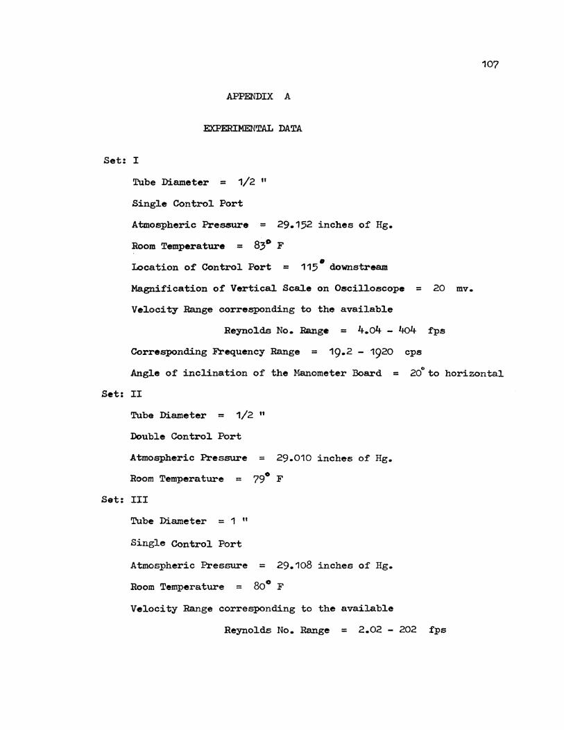
APPENDIX A

EXPERIMENTAL DATA

Set: I

Tube Diameter = 1/2 "

Single Control Port

Atmospheric Pressure = 29.152 inches of Hg.

Room Temperature = 83D F

Location of Control Port = 0 115 downstream

Magnification of Vertical Scale on Oscilloscope = 20 mv.

Velocity Range corresponding to the available

Reynolds No. Range = 4.o4 - 4o4 fps

Corresponding Frequency Range = 19.2 - 1920 cps

107

Angle of inclination of the Manometer Board = 20° to horizontal

Set: II

Tube Diameter = 1/2 "

Double Control Port

Atmospheric Pressure = 29.010 inches of Hg.

Room Temperature = 79° F

Set: III

Tube Diameter = 1 "

Single Control Port

Atmospheric Pressure = 29.108 inches of Hg.

Room Temperature =

Velocity Range corresponding to the available

Reynolds No. Range = 2.02 - 202 fps

Set Run % Wind Tunnel No. No. opening

I. 1. 25

2. 37~

3. 50 4. 75

5· 100

II. 6. 25

7- 37~

8. 50 9. 75

10. 100

III. 11. 25 12. 37/2 13. 50 14. 75 15. 100

IV. 16. 25 17. 3712 18. 50

19. 75 20. 100

Table V. Vortex Frequency and Pitot tube Velocity Measurements

Time setting on No. of cycles on Vortex Frequency Vel. head Vel. head scope m. sec. scope screen 'f' cps inclined Vert.

in. in.

5 7~ 150 0.65 0.222

5 1012 210 1.30 0.445 5 14 280 2.00 0.685 5 17 34o 3.20 1.095 5 19 38o 4.10 1.4o5 5 712 150 0.50 0.171

5 1012 210 1.05 0.360

5 13 260 1.70 0.582

5 16 320 2.75 0.942

5 18 370 3.60 1.232 20 12 ;2 62.5 0.50 0.171 10 10~ 105 1.05 0.360 10 12/2 125 1.70 0.582

5 8 160 2.75 0.94o

5 9 180 3.50 1.20 20 1414 71.2 0.45 0.154 10 1014 102.5 1.00 0.342 10 13~ 135 1.60 0.547

5 8 Y4 165 2.6o 0.890

5 9~ 190 3.60 1.23 ----

Pitot tube velocity

fps

32.313

45.765

56.794 71.846 81.416

28.322

41.104

52.279 66.541

76.127

28.302

41.073

52.239 66.421

75.071 27.027

4o.287

50.963

65.035 t> 76.488

I

I

I

I

-.lo

0 OJ

Set: IV

Tube Diameter = 1 11

Double Control Port

Atmospheric Pressure =28.902 inches of Hg.

R T t 83o F com empera ure = The experimental data to measure Vortex Frequency and

Pitot tube Velocity appears in Table V. consisting of the above

four sets. Figures A1 and A2 are the pictures to evaluate the

vortex frequencies for the test run no. 2 and 20.

Evaluating PS' the Static Pressure in the Test Section of the

Wind Tunnel:

From the pi tot tube data (Table VI. ) A P, the velocity head

109

and (PS-P ) are noted, v1here P is the ambient pressure. A straight e e

line plot with these two variables is then used as a reference to

determine PS for the previous data (knowing AP and the atmospheric

pressure corresponding to any set, PS can easily be evaluated, the

results appear in Table VI.). The knowledge o:f P S is necessary in

order to have an accurate estimate of air density inside the test

section which was used to evaluate different Reynolds No. corresponding

to each run in the data.

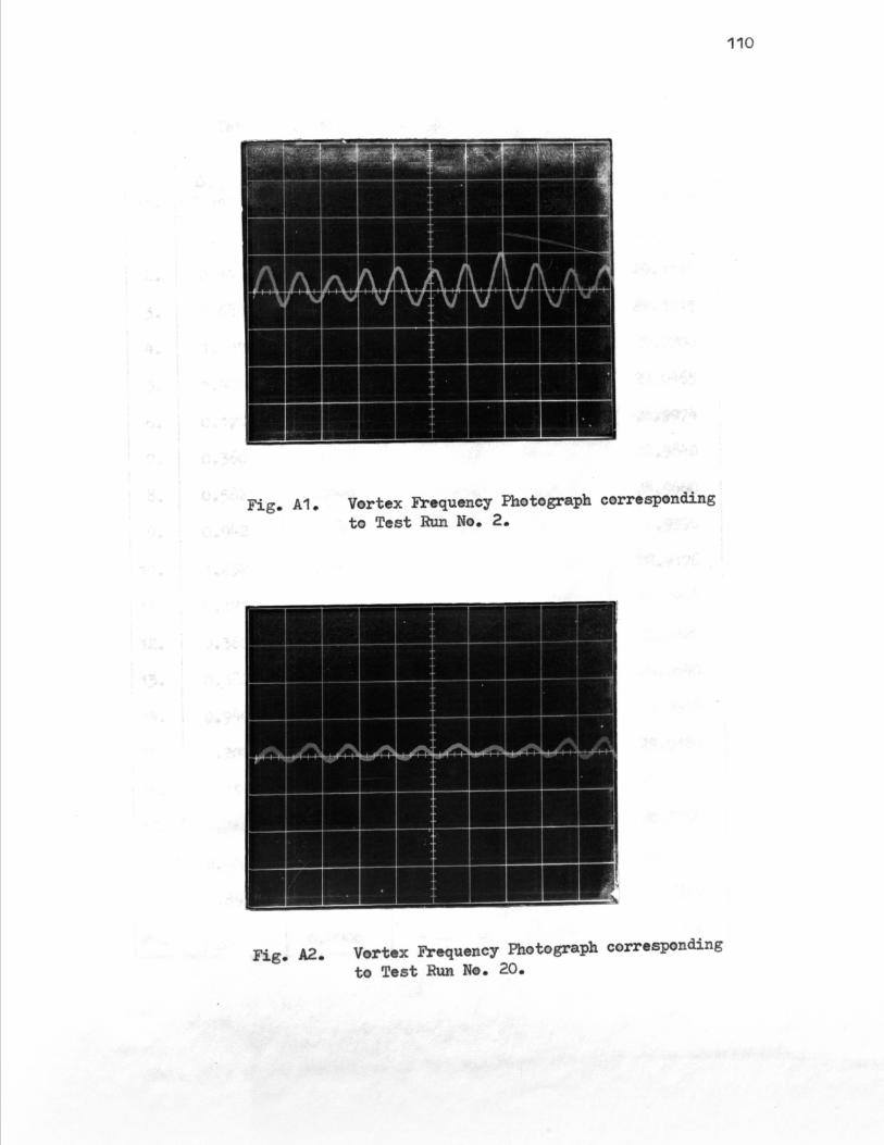
Fig. A1. Vortex Frequency Photograph corresponding to Test Run No. 2.

Fig. A2. Vortex Frequency Photograph corresponding to Test Run Ne. 20.

110

111

Table VI. Pitot tube Data

Run AP, in. AP, in. (P8-P ) p p

No. of water of Hg. in. ofeHg. in. 8r Hg. in. o¥ Hg.

1. 0.222 0.0156 - 0.016 29.152 29.136

2. 0.445 0.0328 - 0.0332 29.152 29.1198

3. 0.685 0.0505 - 0.0505 29.152 29.1015

4. 1.095 0.0805 - 0.0820 29.152 29.0700

5. 1.405 0.1035 - 0.1055 29.152 29.0465

6. 0.171 0.0126 - 0.0126 29.010 28.9974

7- 0.360 0.0258 - 0.0260 29.010 28.9840

8. 0 • .582 0.0428 - o.o44o 29.010 28.9660

9. 0.942 0.0694 - 0.0704 29.010 28.9396

10. 1.232 0.0908 - 0.0924 29.010 28.9176

11. 0.171 0.0126 - 0.0132 29.108 29.0948

12. 0.360 0.0258 - 0.0260 29.108 29.0820

13. 0.582 0.0428 - o.o44o 29.108 29.0640

14. 0.940 0.0692 - 0.0712 29.108 29.0368

15. 1.200 o.o884 - 0.0900 29.108 29.0180

16. 0.154 0.0113 - 0.0114 28.902 28.8906

17. 0.342 0.0252 - 0.0260 28.902 28.8760

18. 0.547 o.o4o3 - 0.0410 28.902 28.8610

19. 0.89 0.0655 - o.o66o 28.902 28.8360

20. 1.23 0.0906 - 0.0912 28.902 28.8108

APPENDIX B

DRAG FORCE .AND VORTEX FRE:XtUENCY RELATION

CD' tle coefficient of drag is given by;

2 CD = D I~ .P.V .A

where

or,

also

or

D = Drag force per unit length of sensor tube

p = I>ensi ty of Air

V = Velocity of Air

A = Projected area per

D = ( ~.P.A. CD ) • v2

s = f.d I v

v = f.d I s

feet length of sensor tube

112

(B-1)

(B-2)

Substituting the value of 'V' from equation (B-2) in (B-1),

D =

=

2 ( ~.P.A. CD).( f.~s ) 2

p A.CD.d • f2

2. s2

It is known that, P ~Constant

Therefore,

where

A = Constant

CD ~ Constant

d = Constant

S '::! Constant

= K.f2 2 2 K = P.A.CD.d /2.S '

S= 0.2058

Table VII. shows the values of 'K' and hence the drag force experienced.

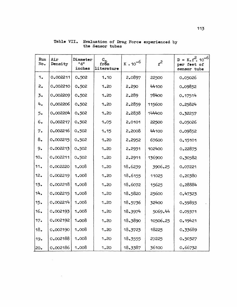
Run No.

1.

2.

3.

4.

5.

6.

7.

8.

9.

10.

11.

12.

13.

14.

15.

16.

17.

18.

19.

20.

113

Table VII. Evaluation of Drag Force experienced by the Sensor tubes

Air Diameter CD 2 -6

K • 10-6 f2 D = K.f • 10

Density I d I from per feet of inches literature sensor tube

0.002211 0.502 1.10 2.0897 22500 0.05026

0.002210 0.502 1.20 2.290 44100 0.09852

0.002209 0.502 1.20 2.289 784oo 0.17514

0.002206 0.502 1.20 2.2859 115600 0.25824

0.002204 0.502 1.20 2.2838 144400 0.32257

0.002217 0.502 1.05 2.0101 22500 0.0,5026

0.002216 0.502 1.15 2.2008 44100 0.09852

0.002215 0.,502 1.20 2.2952 67600 0.15101

0.002213 0.502 1.20 2.2931 102400 0.22875

0.002211 0.502 1.20 2.2911 136900 0.30582

0.002220 1.008 1.20 18.6239 3906.25 0.07221

0.002219 1.008 1.20 18.6155 11025 0.20380

0.002218 1.008 1.20 18.6072 15625 0.28884

0.002215 1.008 1.20 18.5820 25600 0.47323

0.002214 1.008 1.20 18.5736 324oo 0.59893

0.002193 1.008 1.20 18.3974 .5069.44 0.09371

0.002192 1.008 1.20 18.3890 10,506.25 0.19421

0.002190 1.008 1.20 18.3723 18225 0.33689

0.002188 1.008 1.20 18.3555 27225 0.50327

0.002186 1.008 1.20 18.3387 36100 0.66732

• ~ .6 ~ ~

m .5 '-

p::. g fa til .4

~

§ ; .}r ~ .2

2 (!)

~ .1

I

I

For 1 11 Tube

For 1/2 " Tube

\

63,000 83,000 103,000 123,000 143,000 163,000 (FRF.XiUENCY)2

Fig. B1. A Plot of Drag Force experienced by Sensor tubes vs. Square of the Vortex Frequency

~ ~

~

115

Defining a new constantS':

In the present work it is assumed that Strouhal No. remains

constant in the Reynolds No. range of 103 to 105. Fage and Johansenl28]

have made an interesting observation by defining a new constant S',

in place of Strouhal No. It is defined as,

S' = f.d'/V (B-3)

where

d' = distance between the free vortex layers

instead of the usual cylinder diameter

V = Stream Velocity

f = Frequency of vortices shed

S' was found to be rising till R = 300 and after that it was e

practically constant.

S' = 0.14o

= 0.143

at R = 300 e

at R = 20,000+ e

In evaluating S', f and V are already known and d' is related

empirically to '1', the distance between the two consecutive vortices

in the same row.

d'/1 = 0.281

f, the vortex frequency could also be written as;

v - u f =

1

where 'u' is the velocity of vortices with respect to the

flowing liquid.

From equations (B-4) and (B-5),

d' = 0.281 • v- u

f

(B-4)

(B-5)

116

Therefore, s• is given by;

f v - u S' = v 0.281 f

0.281 1 u (B-6) = - v

In the above expression to evaluateS', the problem lies in the

measurement of 'u', the velocity of vortices moving downstream.

Assuming a value of 0.142 for S', d' the distance between free

vortex layers for the experimental data has been calculated (Table VIID

using equation (B-3).

Table VIII. Evaluation of distance between free vortex layers for the Sensor tubes

Run d' Run d' Run d' Run d' No. inches No. inches No. inches No. inches

1. 0.367 6. 0.322 11. 0.770 16. 0.653

2. 0.372 7. 0.334 12. 0.678 17. 0.670

3. 0.342 8. 0.341 13. 0.712 18. 0.642

4. 0.360 9. 0.355 14. 0.706 19. 0.675

5- 0.365 10. 0.352 15. 0.717 20. 0.685

An interesting fact is obtained from equation (B-6) and

assuming a value of 0.142 for s•.

or,

0.142 0.283

u v =

= 1 -

1/2

u v = 1

2

The above equation shows that in the Reynolds No. range of 300

+ to 20,000 the velocity of vortices moving downstream remains

half of the main stream flow velocity.

Fage and Johansen (28] have claimed the new constant S' could

be a better choice in place of the usual Strouhal No. Also, as a

follow up analysis, the calculation of' d' ', could be a valuable

set of data for the further work as regards the vortices shedding

structure is concerned for a particular tube diameter. Once d'

is found accurately for a particular size tube, f can be measured

by the technique presently used and S' is already known to be

constant for a pre-determined velocity range, the velocity could

thus, be estimated with a better precision.

117