Mysteries of Engineering Fluid Mechanicsstubley/Special_Topics/Fluid... · Mysteries of Engineering...
81
Mysteries of Engineering Fluid Mechanics Gordon D. Stubley Mechanical Engineering Department University of Waterloo Waterloo ON N2L 3G1 CANADA email: [email protected] November 30, 2003
Transcript of Mysteries of Engineering Fluid Mechanicsstubley/Special_Topics/Fluid... · Mysteries of Engineering...
Mysteries of Engineering Fluid Mechanics
Gordon D. StubleyMechanical Engineering Department
University of WaterlooWaterloo ON N2L 3G1
CANADAemail: [email protected]
November 30, 2003

2
Contents
1 The Fate of Sinking Tea Leaves 11.1 The Mystery . . . . . . . . . . . . . . . . . . . . . . . . . . . 11.2 Model Flow 1 . . . . . . . . . . . . . . . . . . . . . . . . . . . 1
1.2.1 Description of Flow Conditions . . . . . . . . . . . . . 11.2.2 Exploration . . . . . . . . . . . . . . . . . . . . . . . . 3
1.3 Model Flow 2 . . . . . . . . . . . . . . . . . . . . . . . . . . . 101.3.1 Description of Flow Conditions . . . . . . . . . . . . . 101.3.2 Exploration . . . . . . . . . . . . . . . . . . . . . . . . 10
1.4 Further Exploration . . . . . . . . . . . . . . . . . . . . . . . 151.4.1 Annotated Reading List . . . . . . . . . . . . . . . . . 16
2 The Extra Shock Wave 192.1 The Mystery . . . . . . . . . . . . . . . . . . . . . . . . . . . 192.2 Model Flows . . . . . . . . . . . . . . . . . . . . . . . . . . . 20
2.2.1 Description of Flow Conditions . . . . . . . . . . . . . 202.2.2 Exploration . . . . . . . . . . . . . . . . . . . . . . . . 21
2.3 Further Exploration . . . . . . . . . . . . . . . . . . . . . . . 272.3.1 Annotated Reading List . . . . . . . . . . . . . . . . . 29
3 The Corner Attraction 313.1 The Mystery . . . . . . . . . . . . . . . . . . . . . . . . . . . 313.2 Model Flows . . . . . . . . . . . . . . . . . . . . . . . . . . . 33
3.2.1 Description of Flow Conditions . . . . . . . . . . . . . 333.2.2 Exploration . . . . . . . . . . . . . . . . . . . . . . . . 34
3.3 Further Exploration . . . . . . . . . . . . . . . . . . . . . . . 443.3.1 Role of the Turbulence Model . . . . . . . . . . . . . . 443.3.2 Impact of Secondary Flow . . . . . . . . . . . . . . . . 463.3.3 Annotated Reading List . . . . . . . . . . . . . . . . . 48
i
ii CONTENTS
A Sinking Tea Leaf Model Flow Calculations 51A.1 1: Spinning Flow Above an Infinite Plate . . . . . . . . . . . 51A.2 2: Flow in a Container with a Spinning Lid . . . . . . . . . . 53A.3 3: Flow above an Infinite Spinning Plate . . . . . . . . . . . . 53A.4 4: Vortex Breakdown Flow in a Container . . . . . . . . . . . 53A.5 5: Turbulent Flow in a Container . . . . . . . . . . . . . . . . 55
B Extra Shock Wave Model Flow Calculation 57B.1 Physical Models and Boundary Conditions . . . . . . . . . . . 58B.2 Mesh . . . . . . . . . . . . . . . . . . . . . . . . . . . . . . . . 59B.3 Discretization and Convergence Parameters . . . . . . . . . . 59B.4 Computer Results . . . . . . . . . . . . . . . . . . . . . . . . 60
C Corner Attraction Model Flow Calculation 61C.1 Physical Models and Boundary Conditions . . . . . . . . . . . 61C.2 Mesh . . . . . . . . . . . . . . . . . . . . . . . . . . . . . . . . 63C.3 Discretization and Convergence Parameters . . . . . . . . . . 65C.4 Comparison to Experiment and Other Simulations . . . . . . 65C.5 Computer Results . . . . . . . . . . . . . . . . . . . . . . . . 68
List of Figures
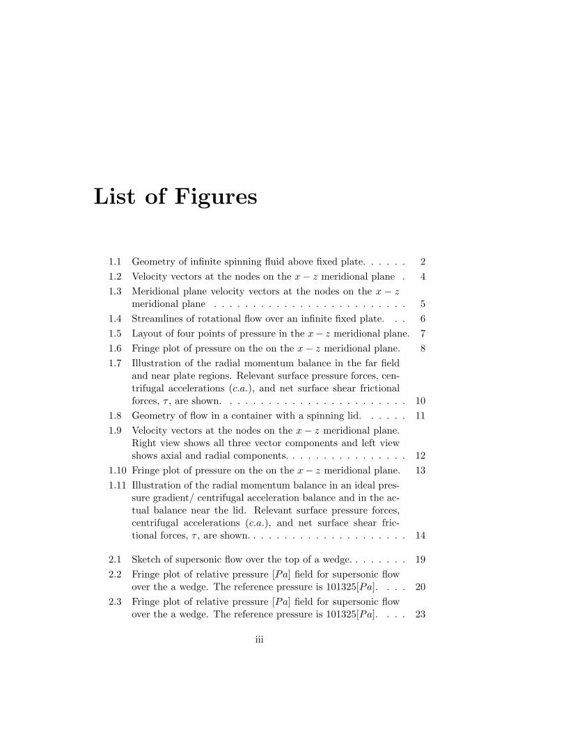
1.1 Geometry of infinite spinning fluid above fixed plate. . . . . . 21.2 Velocity vectors at the nodes on the x− z meridional plane . 41.3 Meridional plane velocity vectors at the nodes on the x − z
meridional plane . . . . . . . . . . . . . . . . . . . . . . . . . 51.4 Streamlines of rotational flow over an infinite fixed plate. . . 61.5 Layout of four points of pressure in the x− z meridional plane. 71.6 Fringe plot of pressure on the on the x− z meridional plane. 81.7 Illustration of the radial momentum balance in the far field
and near plate regions. Relevant surface pressure forces, cen-trifugal accelerations (c.a.), and net surface shear frictionalforces, τ , are shown. . . . . . . . . . . . . . . . . . . . . . . . 10
1.8 Geometry of flow in a container with a spinning lid. . . . . . 111.9 Velocity vectors at the nodes on the x − z meridional plane.
Right view shows all three vector components and left viewshows axial and radial components. . . . . . . . . . . . . . . . 12
1.10 Fringe plot of pressure on the on the x− z meridional plane. 131.11 Illustration of the radial momentum balance in an ideal pres-
sure gradient/ centrifugal acceleration balance and in the ac-tual balance near the lid. Relevant surface pressure forces,centrifugal accelerations (c.a.), and net surface shear fric-tional forces, τ , are shown. . . . . . . . . . . . . . . . . . . . . 14
2.1 Sketch of supersonic flow over the top of a wedge. . . . . . . . 192.2 Fringe plot of relative pressure [Pa] field for supersonic flow
over the a wedge. The reference pressure is 101325[Pa]. . . . 202.3 Fringe plot of relative pressure [Pa] field for supersonic flow
over the a wedge. The reference pressure is 101325[Pa]. . . . 23
iii

iv LIST OF FIGURES
2.4 Fringe plot of relative pressure [Pa] field for supersonic flowover the a wedge with free slip walls. The reference pressureis 101325[Pa]. . . . . . . . . . . . . . . . . . . . . . . . . . . . 23
2.5 Fringe plot of the cross-stream (v) velocity [m s−1] field forsupersonic flow over a wedge. . . . . . . . . . . . . . . . . . . 24
2.6 Fringe plot of the cross-stream (v) velocity [m s−1] field forsupersonic flow over a wedge with free slip walls. . . . . . . . 24
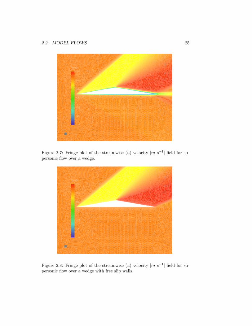
2.7 Fringe plot of the streamwise (u) velocity [m s−1] field forsupersonic flow over a wedge. . . . . . . . . . . . . . . . . . . 25
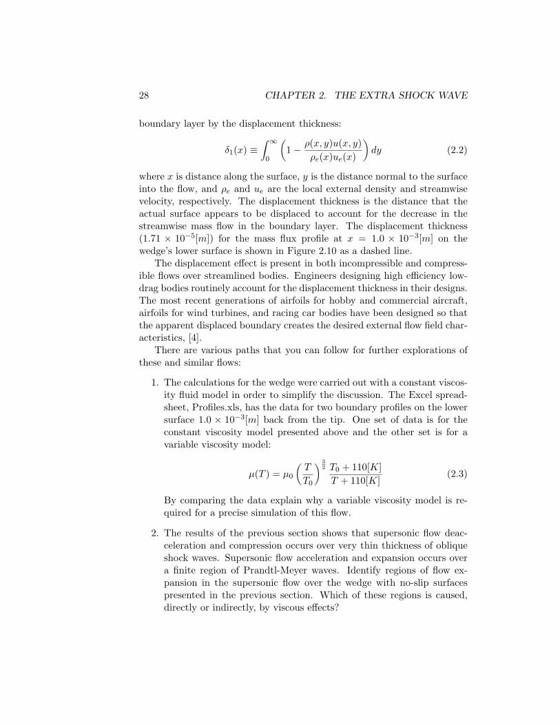
2.8 Fringe plot of the streamwise (u) velocity [m s−1] field forsupersonic flow over a wedge with free slip walls. . . . . . . . 25
2.9 Sketch showing the control volume surrounding the boundarylayer on the lower boundary of the wedge. . . . . . . . . . . . 26
2.10 Mass flux, ρu, profiles near the lower boundary of the wedgefor x = 0[m] and x = 1.0 × 10⁻³[m] distances from the tip.The mass flux is normalized by the external flow mass flux,ρeue. . . . . . . . . . . . . . . . . . . . . . . . . . . . . . . . 27
2.11 Schlieren photograph of air at Mach number =1.965 over asharp 10.1◦ wedge. The lower surface is tilted downwards ata slight angle of 0.3◦. Scan of the photograph presented byVan Dyke[20]. Original photographs and measurements weremade by Bardsley and Mair[1]. . . . . . . . . . . . . . . . . . 29
3.1 Wireframe model of a square duct illustrating the develop-ment of the velocity profile on the y = 0 centre-plane. . . . . 31
3.2 Fringe plot of the fully-developed velocity profile of laminarflow through a square duct. The flow direction is out of thepage. . . . . . . . . . . . . . . . . . . . . . . . . . . . . . . . . 32
3.3 Fringe plot of the fully developed velocity profile of turbulentflow through a square duct. . . . . . . . . . . . . . . . . . . . 33
3.4 Fringe plots of fully developed axial velocity profiles througha square duct. . . . . . . . . . . . . . . . . . . . . . . . . . . . 35
3.5 Vector plots of cross-stream velocity for fully developed flowsin the upper right quadrant of the square duct. . . . . . . . . 36
3.6 Fringe plots of x vorticity component for fully developed flowsin the upper right quadrant of the square duct. . . . . . . . . 37
3.7 Fringe plots of the y normal stress component for fully devel-oped flows in the upper right quadrant of the square duct. . . 38
3.8 Fringe plots of the z normal stress component for fully devel-oped flows in the upper right quadrant of the square duct. . . 39
LIST OF FIGURES v
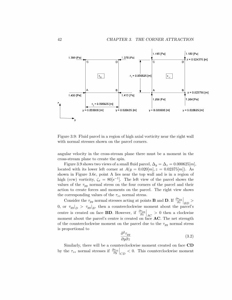
3.9 Fluid parcel in a region of high axial vorticity near the rightwall with normal stresses shown on the parcel corners. . . . . 42
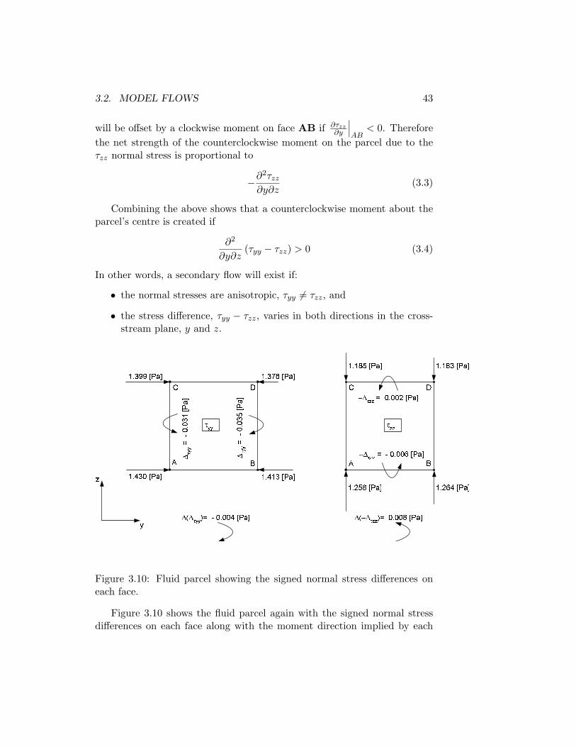
3.10 Fluid parcel showing the signed normal stress differences oneach face. . . . . . . . . . . . . . . . . . . . . . . . . . . . . . 43
A.1 Flow visualization of the centreline vortex as reported byEscudier[5]. The complete depth of the cylinder and the cen-tre 34% of the diameter of the container is shown. . . . . . . 54
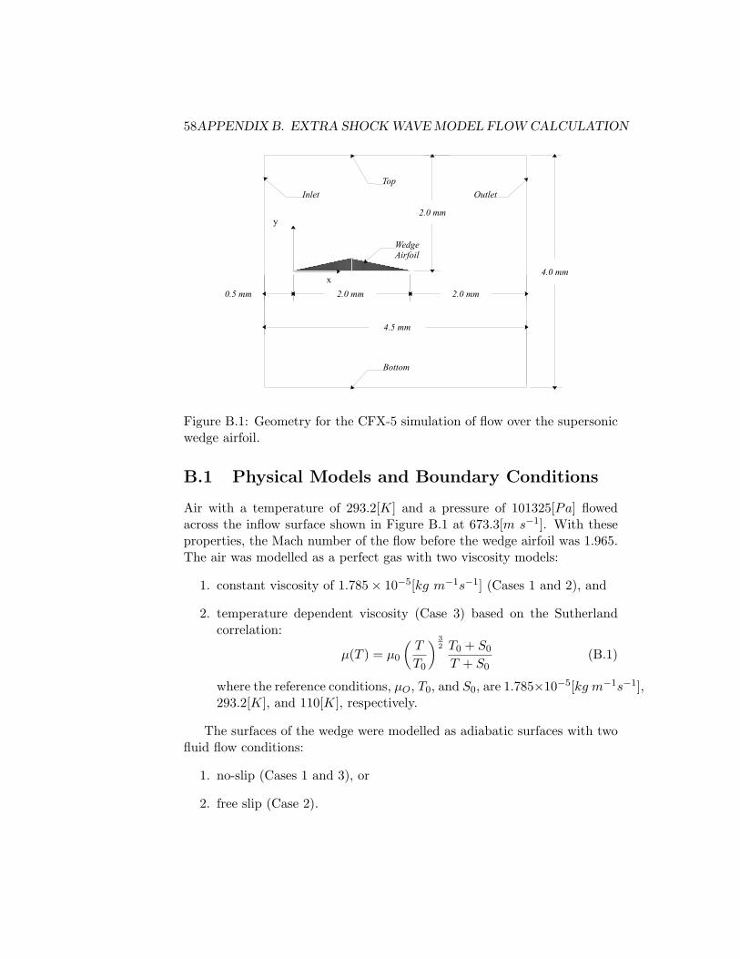
B.1 Geometry for the CFX-5 simulation of flow over the super-sonic wedge airfoil. . . . . . . . . . . . . . . . . . . . . . . . . 58
C.1 Geometry for the CFX-5 simulation of fully-developed flow insquare duct. . . . . . . . . . . . . . . . . . . . . . . . . . . . . 62
C.2 Variation of normalized cross-stream flow speed, Vc−s, alongthe corner diagonal. Normalization is with respect to the wallshear velocity, u?. The y coordinate is shown in Figure C.1. . 67

vi LIST OF FIGURES

Preface
One of the realities of the flow of fluids found in most industrial settings,is that the flow patterns and physics are much more complex than thoseof the model flows presented in undergraduate texts on engineering fluidmechanics. The chapters that follow give you an opportunity to increaseyour ability to understand and control these complex fluid flows.
Each chapter is presented as a mystery which is unraveled as the chapterprogresses. The unraveling of the mystery will involve an exploration ofactual flows that can be easily set up and virtual flow fields obtained bycomputer simulation using computational fluid dynamics (CFD) technology.
The presentation of each mystery has been designed to give ample op-portunity for you to solve the mystery by exploring the flow fields. Take thetime to see all of the features in each flow and to identify the relevant flowkinematics, forces, and dynamics.
Best wishes for an enjoyable learning experience.
vii

viii LIST OF FIGURES
Chapter 1
The Fate of Sinking TeaLeaves
1.1 The Mystery
Tea leaves are added to a beaker of still cold water. As the leaves get soggy,they begin to sink to the bottom of the beaker. This indicates that the tealeaves are heavier than water.
After most of the leaves have sunk to the bottom, the water in the beakeris stirred in either a clockwise or counter-clockwise direction. Where willthe leaves on the bottom of the beaker collect - near the outer wall or nearthe middle?
Those of you that set up this simple flow will notice that the tea leavestend to move towards the middle of the beaker. Why doesn’t centrifugalaction throw the leaves towards the outer wall?
1.2 Model Flow 1
1.2.1 Description of Flow Conditions
One of the simplest imaginable spinning flows is that of a large region offluid spinning with a uniform angular velocity, ω about the z axis. The fluidis above a large fixed plate that lies in the x−y plane as shown in Figure 1.1.
It is natural to use a cylindrical r− θ− z coordinate system for spinningflows where the z axis coincides with the axis of rotation. The three compo-nents of the velocity in this coordinate system are the radial, Vr, tangential,Vt, and the axial, Va velocities in the r, θ and z directions, respectively. A
1

2 CHAPTER 1. THE FATE OF SINKING TEA LEAVES
Figure 1.1: Geometry of infinite spinning fluid above fixed plate.
meridional plane is a plane which contains the axis of rotation and is sweptaround that axis.
The pictures which follow show the flow of water with nominal STPproperties in a region which extends radially from the axis of rotation toa radius of 0.025[m] and vertically from the plate to a height of 0.01[m].The density and dynamic viscosity of the water are 1000[kg m−3] and 1.0×10⁻³[kg m−1s−1], respectively. The rotation rate is 1[rad s−1] or just under10[rpm]. The simulated velocity and pressure fields are presented on auniform mesh with 11 nodes in the radial direction (node spacing of ∆r =0.0025[m]) and with 21 nodes in the axial direction (node spacing of ∆z =0.0005[m]).
1.2. MODEL FLOW 1 3
1.2.2 Exploration
Kinematic Features
Figure 1.2 shows the three-dimensional velocity vectors plotted on the x− zmeridional plane. For this flow, it is sufficient to focus on a meridional planebecause the flow field does not vary in the tangential direction. Can you seethe rotational nature of the velocity field? What other characteristics of thevelocity field can you discern from this figure?
Did you notice that:
• the velocity along the top is almost aligned with the tangential direc-tion and varies linearly as expected for solid body rotation. Note thatvt = ωr so that at the outer edge the tangential velocity is 0.025[m s−1]as indicated by the red colour of the velocity vectors near the outertop corner of the region;
• the velocity field becomes independent of distance in the axial direction(or in other words the axial gradient of the velocity approaches zero,∂~V∂z ≈ 0) far above the fixed plate,
• the tangential velocity goes to zero as the plate is approached indicat-ing that the no-slip condition prevails on the plate,
• the layer of fluid immediately above the fixed plate is moving towardsthe axis of rotation. This negative radial velocity component is largestnear the outer edge and decreases towards the axis of rotation;
• there is a layer of fluid in the middle which appears to be moving awayfrom the axis of rotation, and
• the shape of each column of velocity vectors is similar?
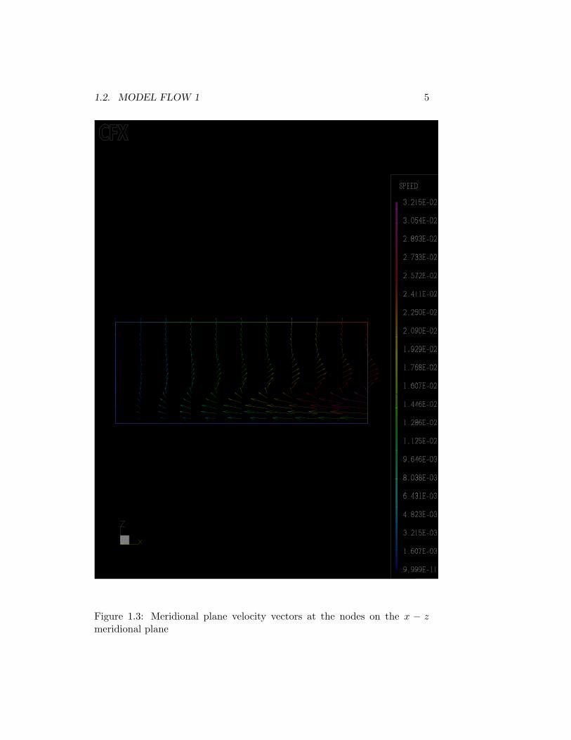
Figure 1.3 shows a two-dimensional plot of the radial and axial velocitycomponents on the x − z meridional plane. Use this meridional plot todiscover more detail about the radial flow observed above. How strong isthe radial flow? Is the velocity far above the fixed plate strictly in thetangential direction?
With this level of detail, you should now notice that:
• the magnitude of the maximum flow in the meridional plane is just be-low 0.015[m s−1] or just under half of the maximum tangential speed,

4 CHAPTER 1. THE FATE OF SINKING TEA LEAVES
Figure 1.2: Velocity vectors at the nodes on the x− z meridional plane
1.2. MODEL FLOW 1 5
Figure 1.3: Meridional plane velocity vectors at the nodes on the x − zmeridional plane

6 CHAPTER 1. THE FATE OF SINKING TEA LEAVES
• the radial flow, both towards and away from the axis of rotation, isclearly seen, and
• an axial velocity component develops with distance above the plate.Far from the plate, the axial velocity component becomes independentof both radial and axial positions.
These pictures show that there are two views of the velocity field: the topview of a horizontal rotating flow and the side view of flow moving radiallyand axially. This radial/axial flow is known as a secondary flow. The netvelocity field is the superposition of these two views: a velocity field whichhas the dominant solid body rotation portion with a secondary flow.
Figure 1.4 shows the three-dimensional nature of the flow. Streamlinesstarting near the plate on the far left of the flow domain spiral towards thecentreline and upwards as a result of the rotating and secondary flows. Thisflow pattern is consistent with the observation that the heavy tea leavescollected near the centreline at the bottom of the beaker.
−0.025−0.02
−0.015−0.01
−0.0050
0.0050.01
0.0150.02
0.025 −0.02
−0.01
0
0.01
0.02
0
0.002
0.004
0.006
0.008
0.01
y
x
z
Figure 1.4: Streamlines of rotational flow over an infinite fixed plate.
Dynamic Features
The kinematic views of the flow field show that even though the flow geome-try and conditions are very simple, the flow pattern is surprisingly complex.
1.2. MODEL FLOW 1 7
What causes this complexity?
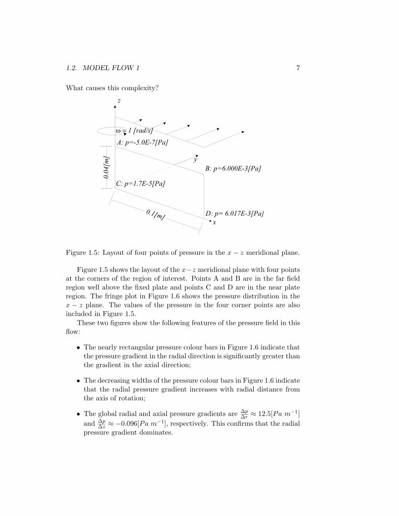
Figure 1.5: Layout of four points of pressure in the x− z meridional plane.
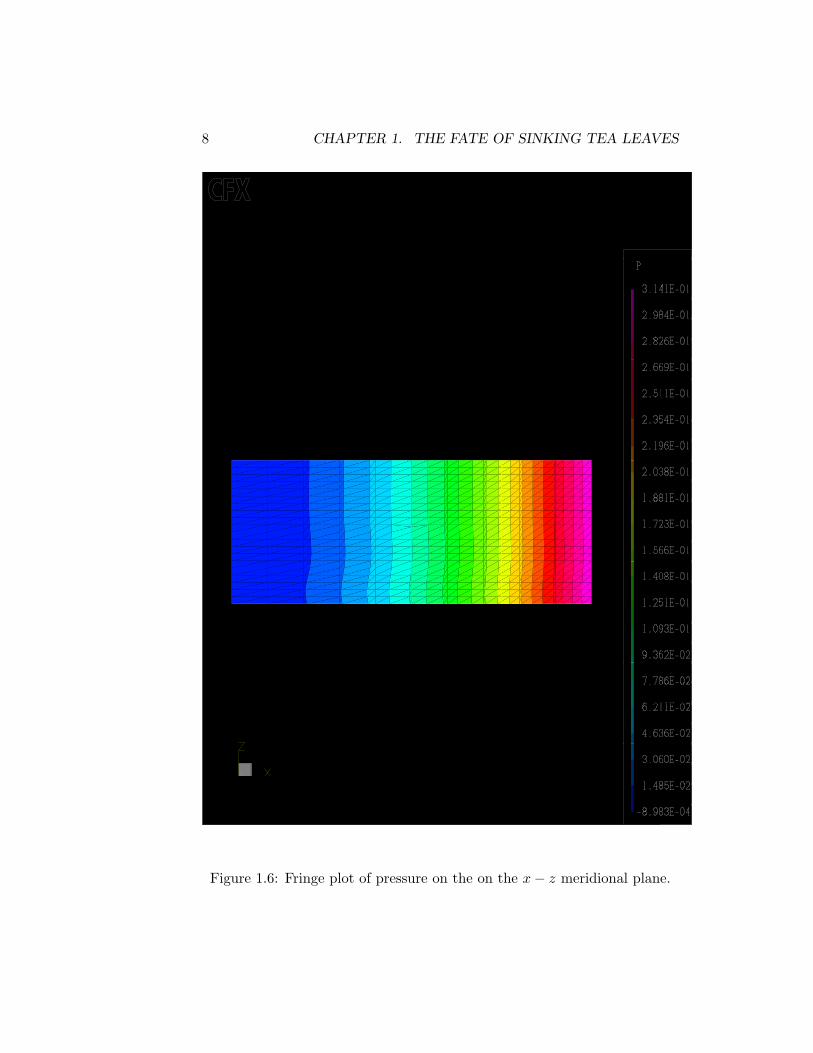
Figure 1.5 shows the layout of the x−z meridional plane with four pointsat the corners of the region of interest. Points A and B are in the far fieldregion well above the fixed plate and points C and D are in the near plateregion. The fringe plot in Figure 1.6 shows the pressure distribution in thex − z plane. The values of the pressure in the four corner points are alsoincluded in Figure 1.5.
These two figures show the following features of the pressure field in thisflow:
• The nearly rectangular pressure colour bars in Figure 1.6 indicate thatthe pressure gradient in the radial direction is significantly greater thanthe gradient in the axial direction;
• The decreasing widths of the pressure colour bars in Figure 1.6 indicatethat the radial pressure gradient increases with radial distance fromthe axis of rotation;
• The global radial and axial pressure gradients are ∆p∆r ≈ 12.5[Pa m−1]
and ∆p∆z ≈ −0.096[Pa m−1], respectively. This confirms that the radial
pressure gradient dominates.
8 CHAPTER 1. THE FATE OF SINKING TEA LEAVES
Figure 1.6: Fringe plot of pressure on the on the x− z meridional plane.
1.2. MODEL FLOW 1 9
The connection between the pressure gradient and the velocity field canbe seen in the radial momentum equation written in cylindrical coordinates:
ρ∂vr
∂t+ ρvr
∂vr
∂r+ ρ
vt
r
∂vr
∂θ+ ρva
∂vr
∂z− ρ
v2t
r
= −∂p
∂r+
µ
[1r
∂
∂r
(r∂vr
∂r
)+
1r2
∂
∂θ
(∂vr
∂θ
)+
∂
∂z
(∂vr
∂z
)− vr
r2− 2
r2
∂vt
∂θ
](1.1)
Throughout the flow domain, the flow field has the following properties:
• the flow is steady, ∂∂t ≈ 0, and
• there is no variation of pressure or velocity in the tangential direction,∂∂θ ≈ 0.
In the far field region(i.e. between Points A and B in Figure 1.5) the velocitygradients in the axial direction are negligible, ∂~V
∂z ≈ 0. Therefore, in the farfield region the radial momentum balance reduces to:
−ρv2t
r= −∂p
∂r(1.2)
or in other words, the radial pressure gradient solely balances the centrifugalacceleration of the tangential velocity field.
Since the tangential velocity is vt = ωr far from the plate (z → ∞) theradial pressure distribution far from the plate is
p(r, z →∞) =ρω2r2
2(1.3)
This parabolic pressure distribution is consistent with the pressure colourbars shown on Figure 1.6 (You should check that this formula predicts thecorrect pressure at Point B).
The observed axial pressure gradient is significantly smaller than theradial pressure gradient. This is consistent with the earlier kinematic ob-servation that the axial velocities far above the plate are very small. Thesmall axial pressure gradient is just sufficient to give fluid parcels a weakaxial acceleration and to move them upwards away from the plate.
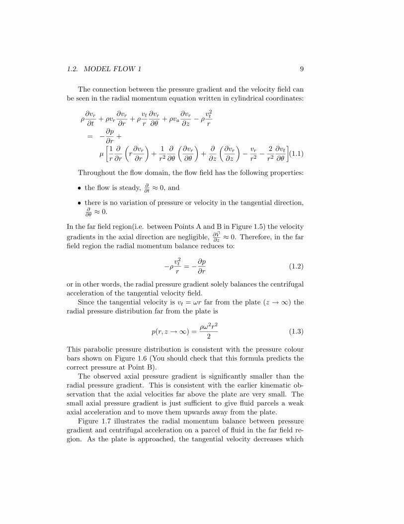
Figure 1.7 illustrates the radial momentum balance between pressuregradient and centrifugal acceleration on a parcel of fluid in the far field re-gion. As the plate is approached, the tangential velocity decreases which
10 CHAPTER 1. THE FATE OF SINKING TEA LEAVES
Figure 1.7: Illustration of the radial momentum balance in the far field andnear plate regions. Relevant surface pressure forces, centrifugal accelerations(c.a.), and net surface shear frictional forces, τ , are shown.
reduces the magnitude of the radial centrifugal acceleration. Since the ra-dial pressure gradient does not change significantly with axial position, animbalance between the radial pressure gradient and the centrifugal acceler-ation exists, as shown in the right hand sketch of Figure 1.7. The radialpressure gradient in the near wall region drives fluid in the radial directiontowards the axis of rotation and the frictional force in the radial directioncreated by this flow restores the radial momentum balance.
1.3 Model Flow 2
1.3.1 Description of Flow Conditions
Figure 1.8 shows the geometry and layout of the second model flow: flowin a cylindrical container with a spinning lid. The container has a radius of0.025[m] and a height of 0.025[m]. The lid of the container is spinning witha rotation rate of ω = 0.64[rad s−1]. The fluid in the container is water withnominal STP properties: ρ = 1000[kg m−3] and µ = 1. × 10−3[kg m−1s−1]and it completely fills the container. The rotation rate was set so that theReynolds number of the flow is Re ≡ ρωR2
µ = 400. With this low Reynoldsnumber you can expect the flow to be laminar.
The simulated flow field is presented on an uniform mesh with 80 nodesin the axial and radial directions.
1.3.2 Exploration
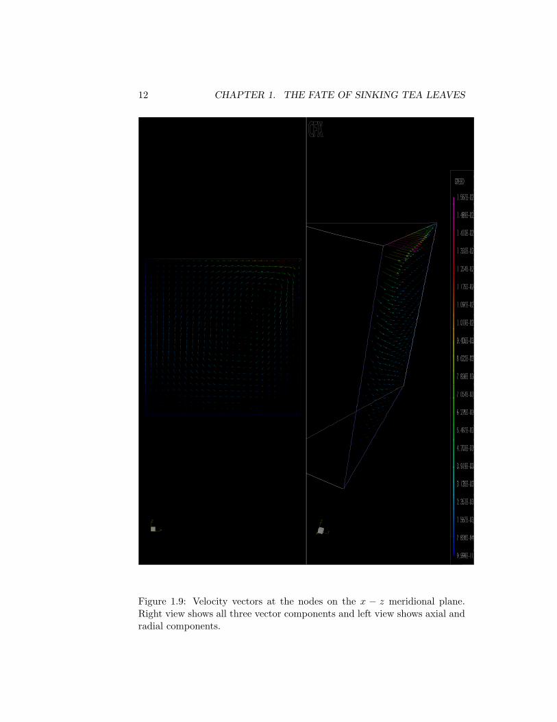
Figure 1.9 shows two views of the velocity field on the x − z meridionalplane. The left view shows the axial and radial velocity components on the

1.3. MODEL FLOW 2 11
Figure 1.8: Geometry of flow in a container with a spinning lid.
meridional plane while the right view shows all three velocity componentson the same plane.
What differences do you notice between this flow field and the infiniteflow field without the container walls?
From the right view showing all the three velocity components, you cannotice:
• the tangential velocity of the lid varies linearly with radius as expected;
• the speed of the fluid drops rapidly with distance away from the lid.The core of the fluid is rotating much more slowly than the lid; and
• the container wall slows down the fluid in its vicinity significantly.
In the left view, which emphasizes the secondary flow, it is clear thatthere is single closed cell of fluid rotating in the meridional plane about thepoint (0.0188[m],0.0[m],0.0183[m])1.
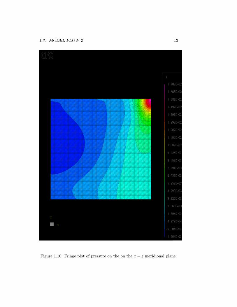
Figure 1.10 shows a fringe plot of the pressure distribution on the x− zmeridional plane. This pressure field is significantly more complex than thatof the infinite flow field. What similarities and differences can you noticebetween this pressure field and that shown in Figure 1.6?
1These values are in excellent agreement with the benchmark prediction of Lugt andHaussling[11]
12 CHAPTER 1. THE FATE OF SINKING TEA LEAVES
Figure 1.9: Velocity vectors at the nodes on the x − z meridional plane.Right view shows all three vector components and left view shows axial andradial components.
1.3. MODEL FLOW 2 13
Figure 1.10: Fringe plot of pressure on the on the x− z meridional plane.

14 CHAPTER 1. THE FATE OF SINKING TEA LEAVES
The most striking feature of the pressure distribution in the containeris the pressure rise near the outer top corner. Some of this pressure rise ispartially due to an artiface of the numerical simulation which assumes thatthere is no gap between the spinning lid and fixed container wall. However, aportion of the pressure rise in the radial direction along the lid balances thecentrifugal acceleration of the fluid near the lid. Since the core of fluid nearthe spinning lid is spinning at a much lower rate than the lid, the pressurein the top corner, 1.8× 10⁻²[Pa] is considerably less than that predicted byEquation 1.3, 0.128[Pa]. Because the radial pressure gradient is less thanthat required to balance the centrifugal acceleration at the lid, a flow fromthe axis of rotation to the outer wall is created along the lid as illustratedin Figure 1.11.
Figure 1.11: Illustration of the radial momentum balance in an ideal pressuregradient/ centrifugal acceleration balance and in the actual balance near thelid. Relevant surface pressure forces, centrifugal accelerations (c.a.), and netsurface shear frictional forces, τ , are shown.
Between the top of container wall and the container bottom there is aconsiderable pressure drop. This axial pressure gradient is required to drivethe fluid from the top to the bottom in the closed circulation cell and toovercome the viscous drag along the container wall.
Even though there is a significant reduction of the radial pressure gra-dient between the top and the bottom of the container, the positive radialpressure gradient on the container bottom drives fluid from the containerwall to the axis of rotation. The radial momentum balance in the near bot-tom region is a balance between the radial pressure gradient and the netviscous shear forces resisting motion in the radial direction.
There is a weak negative axial pressure gradient near the axis of rotationto drive the fluid up from the bottom and towards the top of the container.

1.4. FURTHER EXPLORATION 15
1.4 Further Exploration
In the previous two sections, two model flows have been explored in whicha secondary flow pattern is established by the imbalance between radialpressure gradients and centrifugal accelerations. If either model flow wereseeded with particles slightly heavier than water then these particles wouldcollect at the bottom near the axis of rotation just as the tea leaves did inthe beaker of stirred water.
You can look for similar secondary flow patterns in any situation wherethe flow is rotating. Common examples include flows in centrifugal pumps,in radial flow turbines, in duct and pipe bends, near car brake disks andnear high and low pressure systems in the atmosphere.
Secondary flows can be created by other mechanisms also. For example,secondary flows such as the earth’s large scale atmospheric circulation arecreated by buoyancy forces resulting from temperature variations in the flowfield. Another subtle example is the secondary flow in rectangular ducts thatis driven by an imbalance in the turbulent stresses.
Even if you do not begin to study secondary flows due to other mech-anisms, there is still a lot to be learned about secondary flows in rotatingflows. The following questions and suggestions can help you explore thiscomplex subject in further detail:
1. The flow in the beaker has a free surface between the water and theair. Explain the shape of the water surface that is observed;
2. Explain why clear weather is associated with high pressure systemsand cloudy weather is associated with low pressure systems;
3. Model Flow 3 is a model flow that is similar to Model Flow 1. Inthis model flow, the fluid far away from the plate is at rest and theplate is spinning. Before exploring the simulated flow field, see if youcan estimate the pressure distribution and directions of the axial andradial velocity components. What similarities are there between thismodel flow and Model Flow 2 presented above?
4. Model Flow 3 can be simulated with CFD codes. You will have to takecare in modeling the boundary condition for the top (far field from theplate). A specified total pressure and flow direction is recommendedfor this inflow boundary. Why is it adequate to set a zero static pres-sure condition for the outflow at the outside (R) of the domain?
16 CHAPTER 1. THE FATE OF SINKING TEA LEAVES
5. Model Flow 4 is laminar flow in a container with a slightly higherReynolds number, Re = 1492, and aspect ratio, H/R = 1.5. In whatsignificant way is this flow field dissimilar from that of Model Flow 2(Re = 400)? This flow shows a vortex breakdown;
6. Model Flow 5 is a turbulent flow in a container with a spinning lid,H/R = 1.5 and Re = 2.5× 10⁵. How does the shape of the turbulentflow field’s secondary flow pattern compare to that of Model Flow 4.From this model flow can you see why it is that the tea leaves do notcongregate right on the axis of rotation?
7. The torque, T , required to turn the spinning lid of the container forModel Flows 2,4, and 5, were estimated from CFX-TASCflow simula-tions to be 2.06×10⁻⁷[N m], 1.35×10⁻⁶[N m], and 3.36×10⁻³[N m],respectively. Schlichting[16] provides the following theoretical correla-tions for the torque coefficient, CT ≡ 2T
12ρω2R5 , for a spinning plate in
an infinite flow:
CT =
{3.87Re Re < 5× 10⁴
0.146Re−1/5 Re > 5× 10⁴ (1.4)
Plot the predicted torque coefficients and the experimenatal correla-tions. After noting that the trends of the predicted torque coefficientsclosely matches thoses of the correlations, provide a list of factorsexplaining why the predicted values do not exactly agree with thecorrelations; and
8. Which of the three model flows, 2, 4, or 5, most closely models theflow field that exists in the beaker of stirred water?
1.4.1 Annotated Reading List
There is a large literature on centrifugally driven secondary flows and thevortex structures that are created in theses flows. The following texts andarticles are recommended for further reading:
Schlichting[16], pp. 102-107,225-230, and 647-651 This classic text presentssemi-analytical solutions for several laminar flows involing rotation andempirical theories for turbulent flow near spinning disks. The empha-sis is on quantitative estimation of measures such as the drag torqueon spinning disks,
1.4. FURTHER EXPLORATION 17
Lugt[12], pp.138-145 An excellent description of many flow features ofrotating fluids in containers. The use of mathematics is kept to aminimum and the emphasis is on qualitative description,
Lugt[13], pp.430-435 An updated version of his earlier presentation. Thistext provides a more complete and mathematical presentation of vor-tex theory,
Escudier[7] A comprehensive summary of the important experiments andtheories of the formation and breakdown of vortices in rotating flows,
Escudier[6] A well written article showing five examples of flow machineryin which vortices play a significant role in the machine’s performance,and
Daily and Nece[3] A detailed experimental study of the flow field on thebackface of impellers and the resulting frictional losses.

18 CHAPTER 1. THE FATE OF SINKING TEA LEAVES
Chapter 2
The Extra Shock Wave
2.1 The Mystery
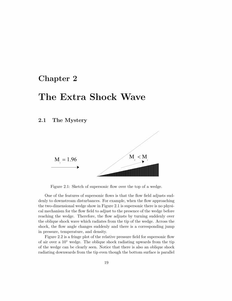
Figure 2.1: Sketch of supersonic flow over the top of a wedge.
One of the features of supersonic flows is that the flow field adjusts sud-denly to downstream disturbances. For example, when the flow approachingthe two-dimensional wedge show in Figure 2.1 is supersonic there is no physi-cal mechanism for the flow field to adjust to the presence of the wedge beforereaching the wedge. Therefore, the flow adjusts by turning suddenly overthe oblique shock wave which radiates from the tip of the wedge. Across theshock, the flow angle changes suddenly and there is a corresponding jumpin pressure, temperature, and density.
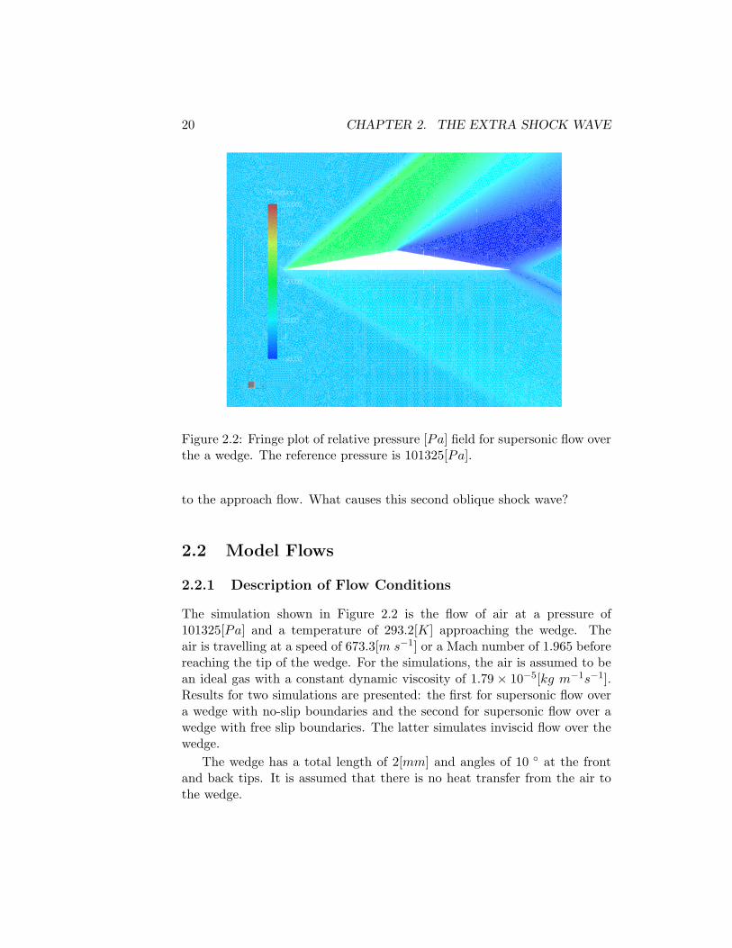
Figure 2.2 is a fringe plot of the relative pressure field for supersonic flowof air over a 10◦ wedge. The oblique shock radiating upwards from the tipof the wedge can be clearly seen. Notice that there is also an oblique shockradiating downwards from the tip even though the bottom surface is parallel
19
20 CHAPTER 2. THE EXTRA SHOCK WAVE
Figure 2.2: Fringe plot of relative pressure [Pa] field for supersonic flow overthe a wedge. The reference pressure is 101325[Pa].
to the approach flow. What causes this second oblique shock wave?
2.2 Model Flows
2.2.1 Description of Flow Conditions
The simulation shown in Figure 2.2 is the flow of air at a pressure of101325[Pa] and a temperature of 293.2[K] approaching the wedge. Theair is travelling at a speed of 673.3[m s−1] or a Mach number of 1.965 beforereaching the tip of the wedge. For the simulations, the air is assumed to bean ideal gas with a constant dynamic viscosity of 1.79 × 10⁻⁵[kg m−1s−1].Results for two simulations are presented: the first for supersonic flow overa wedge with no-slip boundaries and the second for supersonic flow over awedge with free slip boundaries. The latter simulates inviscid flow over thewedge.
The wedge has a total length of 2[mm] and angles of 10 ◦ at the frontand back tips. It is assumed that there is no heat transfer from the air tothe wedge.

2.2. MODEL FLOWS 21
2.2.2 Exploration
Examine the following set of fringe plots showing the relative pressure1 ,cross-stream (v) velocity, and streamwise (u) velocity fields in the vicinityof the wedge. For each field variable two fringe plots are provided: thefirst for flow over no-slip boundaries and the second for flow over free slipboundaries.
On each fringe plot, two reference points are plotted. Above the wedge,a point is shown along the line that radiates at a 40 ◦ angle from the tip.This angle corresponds to the angle of an oblique shock for inviscid flow(flow of a fluid with negligible viscous effects) turning through 10◦. Belowthe wedge, a point is shown along the line that radiates at a 31.4◦ anglefrom the tip. This angle corresponds to the angle of an oblique shock forinviscid flow turning through 1◦.
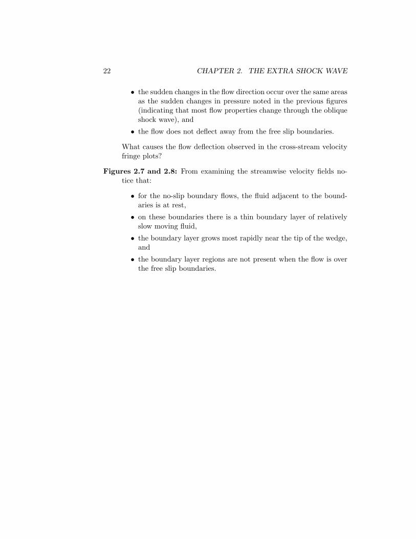
Figures 2.3 and 2.4: From examining the pressure fields notice that:
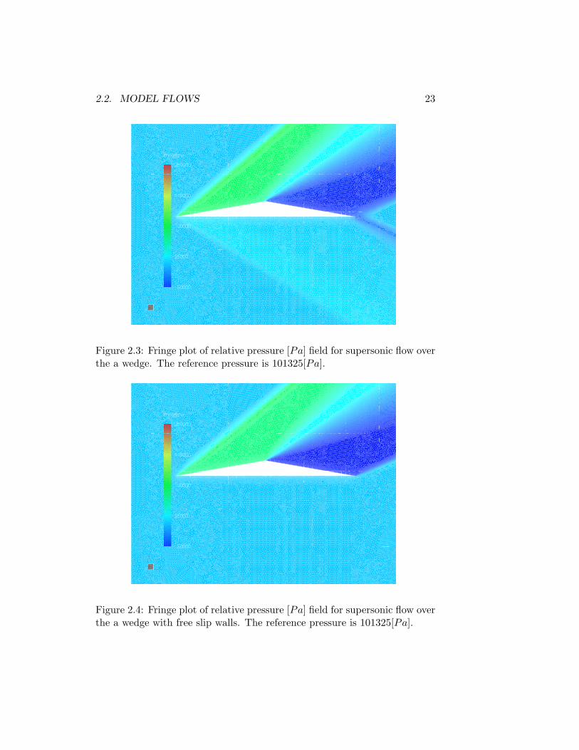
• there is no shock wave radiating from the lower edge of the tipwhen the flow is over free slip boundaries,
• the oblique shock angle above the wedge for the flow over the freeslip boundaries corresponds very closely to that predicted by theoblique shock relations for inviscid flow,
• the oblique shock angle above the wedge for flow over the no-slipboundaries is greater than that predicted by the oblique shockrelations for inviscid flow, and
• the oblique shock below the wedge corresponds closely to anoblique shock of inviscid flow turning through an angle of 1◦.
Figures 2.5 and 2.6: From examining the cross-stream velocity fields no-tice that:
• for the flow over the no-slip boundaries, the flow is clearly de-flected downwards away from the bottom surface of the wedge,
• the magnitude of the deflection is greatest near the tip of thewedge2 and then decreases with distance along the bottom surfaceof the wedge,
1The relative pressure field is referenced to the approach pressure of 101325[Pa]. Arelative pressure of 0[Pa] indicates an undisturbed flow.
2The flow angle is 1◦ downwards near the tip.
22 CHAPTER 2. THE EXTRA SHOCK WAVE
• the sudden changes in the flow direction occur over the same areasas the sudden changes in pressure noted in the previous figures(indicating that most flow properties change through the obliqueshock wave), and
• the flow does not deflect away from the free slip boundaries.
What causes the flow deflection observed in the cross-stream velocityfringe plots?
Figures 2.7 and 2.8: From examining the streamwise velocity fields no-tice that:
• for the no-slip boundary flows, the fluid adjacent to the bound-aries is at rest,
• on these boundaries there is a thin boundary layer of relativelyslow moving fluid,
• the boundary layer grows most rapidly near the tip of the wedge,and
• the boundary layer regions are not present when the flow is overthe free slip boundaries.
2.2. MODEL FLOWS 23
Figure 2.3: Fringe plot of relative pressure [Pa] field for supersonic flow overthe a wedge. The reference pressure is 101325[Pa].
Figure 2.4: Fringe plot of relative pressure [Pa] field for supersonic flow overthe a wedge with free slip walls. The reference pressure is 101325[Pa].

24 CHAPTER 2. THE EXTRA SHOCK WAVE
Figure 2.5: Fringe plot of the cross-stream (v) velocity [m s−1] field forsupersonic flow over a wedge.
Figure 2.6: Fringe plot of the cross-stream (v) velocity [m s−1] field forsupersonic flow over a wedge with free slip walls.
2.2. MODEL FLOWS 25
Figure 2.7: Fringe plot of the streamwise (u) velocity [m s−1] field for su-personic flow over a wedge.
Figure 2.8: Fringe plot of the streamwise (u) velocity [m s−1] field for su-personic flow over a wedge with free slip walls.

26 CHAPTER 2. THE EXTRA SHOCK WAVE
Figure 2.9: Sketch showing the control volume surrounding the boundarylayer on the lower boundary of the wedge.
Why does the boundary layer flow generate a cross-stream flow awayfrom the bottom boundary of the wedge?
The above flow field figures show that there are two flow regions forthe flow over the wedge with no-slip surfaces: a thin boundary layer regionwith appreciable shear strain rates and corresponding shear stresses and anexternal flow region with relatively small gradients except over shock waves.The boundary layer flow region is not present in the flow over the wedgewith slip surfaces.
Figure 2.9 shows a control volume that encloses the boundary layer re-gion over the span of 1.0 × 10⁻³[m] along the lower surface of the wedge.The streamwise, u, velocity component carries mass into this control vol-ume across the left face and out of the control volume across the right face.Figure 2.10 shows the the mass flux, ρu, profiles across the left and rightfaces. It is clear that the total mass flow across the left face:
Total Mass Flow =∫ δ
0ρudy (2.1)
exceeds that across the right face by a significant amount. Since no massflows across the solid boundary, there must be a cross-stream mass flow awayfrom the boundary layer.
The cross-stream mass flow pushes or displaces the freestream or externalflow away from the bottom surface of the wedge. It is this displacement effectthat causes the external flow over the no-slip boundary to turn 1◦ away fromthe wedge. The turning occurs across the weak oblique shock wave radiatingdownwards from the tip. As the boundary growth decreases with distancealong the surface, the flow angle decreases, as can be seen in Figure 2.5.

2.3. FURTHER EXPLORATION 27
0.0e+00
2.0e-05
4.0e-05
6.0e-05
8.0e-05
1.0e-04
1.2e-04
1.4e-04
1.6e-04
0 0.2 0.4 0.6 0.8 1
y[m]
ρuρeue
x = 0[m]
33 33333333333333333
333
33
333
33
33
3
3x = 1.0× 10⁻³[mm]
++ + + + + + +++ ++ +++++
++++++++++
+++
+
+
Figure 2.10: Mass flux, ρu, profiles near the lower boundary of the wedgefor x = 0[m] and x = 1.0 × 10⁻³[m] distances from the tip. The mass fluxis normalized by the external flow mass flux, ρeue.
A boundary layer grows on the top surface of the wedge also. Thisboundary layer causes a displacement effect on the top surface of the wedge.The turning of the external flow that occurs across the top shock must besufficient to turn the flow away from the solid surface plus the displacementeffect. This explains why the oblique shock angle shown in Figure 2.3 isgreater than that predicted by the inviscid flow shock relations. While notshown, the oblique shock angle of 41.75◦ in the flow over the no-slip uppersurface corresponds to a flow turning angle of 11.5◦ which is the flow angleat the outside of the upper surface boundary layer near the wedge tip.
2.3 Further Exploration
The supersonic flow over the wedge, discussed above, illustrates one im-portant consequence of the no-slip condition at solid walls: the boundarydisplacement effect. This effect is quantified along the length of a developing
28 CHAPTER 2. THE EXTRA SHOCK WAVE
boundary layer by the displacement thickness:
δ1(x) ≡∫ ∞
0
(1− ρ(x, y)u(x, y)
ρe(x)ue(x)
)dy (2.2)
where x is distance along the surface, y is the distance normal to the surfaceinto the flow, and ρe and ue are the local external density and streamwisevelocity, respectively. The displacement thickness is the distance that theactual surface appears to be displaced to account for the decrease in thestreamwise mass flow in the boundary layer. The displacement thickness(1.71 × 10⁻⁵[m]) for the mass flux profile at x = 1.0 × 10⁻³[m] on thewedge’s lower surface is shown in Figure 2.10 as a dashed line.
The displacement effect is present in both incompressible and compress-ible flows over streamlined bodies. Engineers designing high efficiency low-drag bodies routinely account for the displacement thickness in their designs.The most recent generations of airfoils for hobby and commercial aircraft,airfoils for wind turbines, and racing car bodies have been designed so thatthe apparent displaced boundary creates the desired external flow field char-acteristics, [4].
There are various paths that you can follow for further explorations ofthese and similar flows:
1. The calculations for the wedge were carried out with a constant viscos-ity fluid model in order to simplify the discussion. The Excel spread-sheet, Profiles.xls, has the data for two boundary profiles on the lowersurface 1.0 × 10⁻³[m] back from the tip. One set of data is for theconstant viscosity model presented above and the other set is for avariable viscosity model:
µ(T ) = µ0
(T
T0
) 32 T0 + 110[K]
T + 110[K](2.3)
By comparing the data explain why a variable viscosity model is re-quired for a precise simulation of this flow.
2. The results of the previous section shows that supersonic flow deac-celeration and compression occurs over very thin thickness of obliqueshock waves. Supersonic flow acceleration and expansion occurs overa finite region of Prandtl-Meyer waves. Identify regions of flow ex-pansion in the supersonic flow over the wedge with no-slip surfacespresented in the previous section. Which of these regions is caused,directly or indirectly, by viscous effects?
2.3. FURTHER EXPLORATION 29
3. Drag on airfoils and other streamlined bodies is caused both by viscousshear action and net pressure forces. The latter is often referred toas form drag. Estimate the form drag on the wedges with no-slip andslip surfaces. Explain the difference in the two estimates.
2.3.1 Annotated Reading List
There is a large literature on boundary layer displacement effects is incom-pressible and compressible flows. The following are recommended for furtherreading:
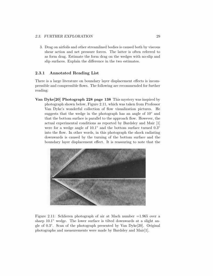
Van Dyke[20] Photograph 228 page 138 This mystery was inspired byphotograph shown below, Figure 2.11, which was taken from ProfessorVan Dyke’s wonderful collection of flow visualization pictures. Hesuggests that the wedge in the photograph has an angle of 10◦ andthat the bottom surface is parallel to the approach flow. However, theactual experimental conditions as reported by Bardsley and Mair [1]were for a wedge angle of 10.1◦ and the bottom surface turned 0.3◦
into the flow. In other words, in this photograph the shock radiatingdownwards is caused by the turning of the bottom surface and theboundary layer displacement effect. It is reassuring to note that the
Figure 2.11: Schlieren photograph of air at Mach number =1.965 over asharp 10.1◦ wedge. The lower surface is tilted downwards at a slight an-gle of 0.3◦. Scan of the photograph presented by Van Dyke[20]. Originalphotographs and measurements were made by Bardsley and Mair[1].
30 CHAPTER 2. THE EXTRA SHOCK WAVE
upper shock angle of 41.8◦ predicted in the simulations of the previoussection is within the range, 40.3◦ − 42.3◦, of upper shock angle thatcan be inferred from the measurements of Bardsley and Mair.
Eppler[4] This text covers the design philosophy and calculation techniquesused to design the high-lift and low drag subsonic airfoils in the 1980’sand 1990’s. The role of the displacement effect and the direct andindirect impact of viscous effects are discussed in detail.
White[21] Chapter 7 Professor White provides a modern perspective onthe physics of compressible boundary layers. The impact of tempera-ture variations on the flow field properties in boundary layers is cov-ered.
Chapter 3
The Corner Attraction
3.1 The Mystery
�
����� ����� � �����
� � �����
� �� �����������
� �����
�
�
� �"! �$#&%'�( �&) �
* ����+ �",�.- u
/
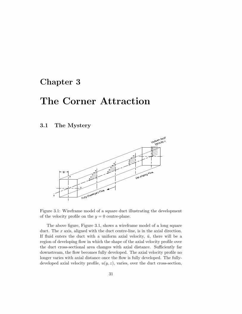
Figure 3.1: Wireframe model of a square duct illustrating the developmentof the velocity profile on the y = 0 centre-plane.
The above figure, Figure 3.1, shows a wireframe model of a long squareduct. The x axis, aligned with the duct centre-line, is in the axial direction.If fluid enters the duct with a uniform axial velocity, u, there will be aregion of developing flow in which the shape of the axial velocity profile overthe duct cross-sectional area changes with axial distance. Sufficiently fardownstream, the flow becomes fully developed. The axial velocity profile nolonger varies with axial distance once the flow is fully developed. The fully-developed axial velocity profile, u(y, z), varies, over the duct cross-section,
31
32 CHAPTER 3. THE CORNER ATTRACTION
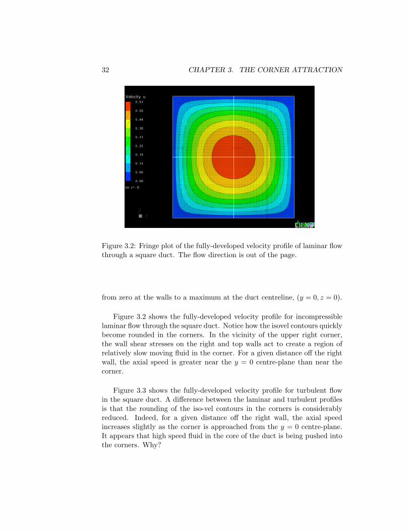
Figure 3.2: Fringe plot of the fully-developed velocity profile of laminar flowthrough a square duct. The flow direction is out of the page.
from zero at the walls to a maximum at the duct centreline, (y = 0, z = 0).
Figure 3.2 shows the fully-developed velocity profile for incompressiblelaminar flow through the square duct. Notice how the isovel contours quicklybecome rounded in the corners. In the vicinity of the upper right corner,the wall shear stresses on the right and top walls act to create a region ofrelatively slow moving fluid in the corner. For a given distance off the rightwall, the axial speed is greater near the y = 0 centre-plane than near thecorner.
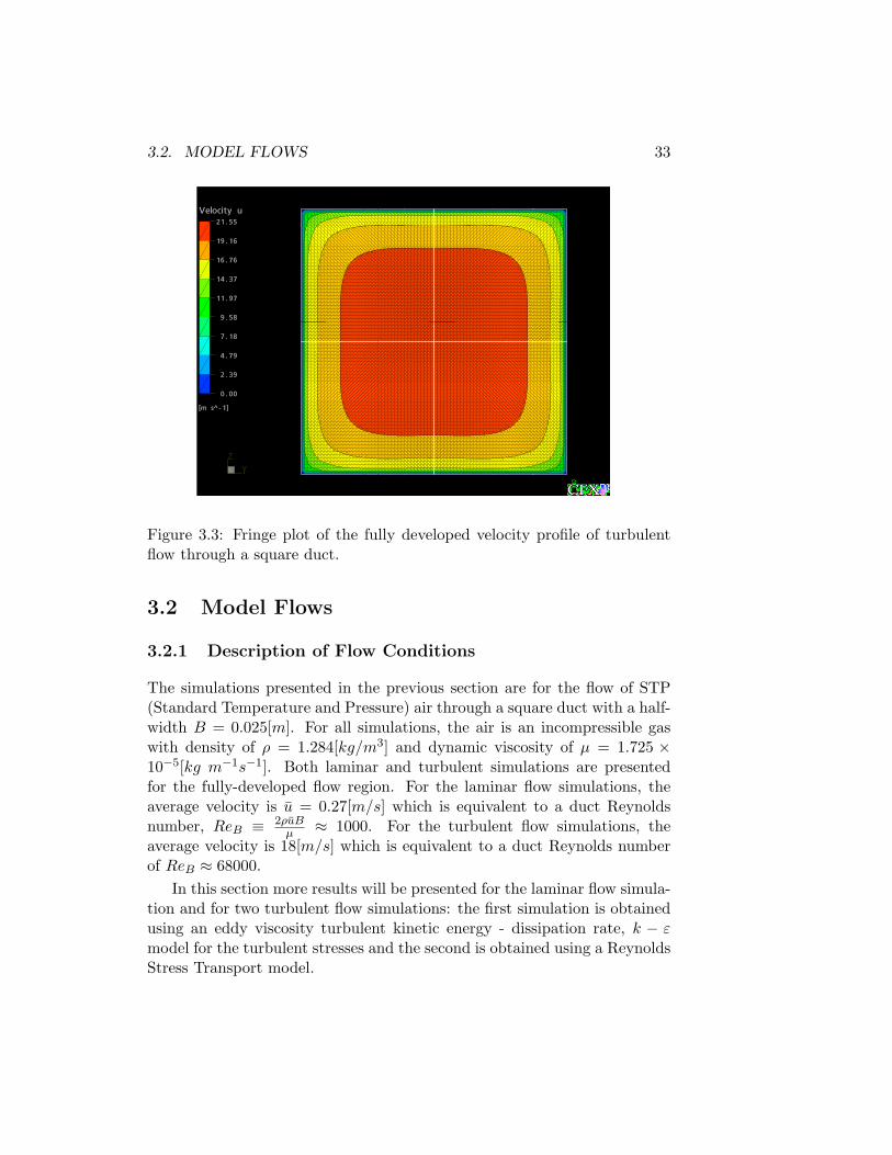
Figure 3.3 shows the fully-developed velocity profile for turbulent flowin the square duct. A difference between the laminar and turbulent profilesis that the rounding of the iso-vel contours in the corners is considerablyreduced. Indeed, for a given distance off the right wall, the axial speedincreases slightly as the corner is approached from the y = 0 centre-plane.It appears that high speed fluid in the core of the duct is being pushed intothe corners. Why?
3.2. MODEL FLOWS 33
Figure 3.3: Fringe plot of the fully developed velocity profile of turbulentflow through a square duct.
3.2 Model Flows
3.2.1 Description of Flow Conditions
The simulations presented in the previous section are for the flow of STP(Standard Temperature and Pressure) air through a square duct with a half-width B = 0.025[m]. For all simulations, the air is an incompressible gaswith density of ρ = 1.284[kg/m3] and dynamic viscosity of µ = 1.725 ×10⁻⁵[kg m−1s−1]. Both laminar and turbulent simulations are presentedfor the fully-developed flow region. For the laminar flow simulations, theaverage velocity is u = 0.27[m/s] which is equivalent to a duct Reynoldsnumber, ReB ≡ 2ρuB
µ ≈ 1000. For the turbulent flow simulations, theaverage velocity is 18[m/s] which is equivalent to a duct Reynolds numberof ReB ≈ 68000.
In this section more results will be presented for the laminar flow simula-tion and for two turbulent flow simulations: the first simulation is obtainedusing an eddy viscosity turbulent kinetic energy - dissipation rate, k − εmodel for the turbulent stresses and the second is obtained using a ReynoldsStress Transport model.
34 CHAPTER 3. THE CORNER ATTRACTION
3.2.2 Exploration
Examine the set of figures on the following pages that show fringe plots ofthe axial velocity, the cross-stream velocity vectors, fringe plots of the xcomponent of the vorticity, and fringe plots for the y and z normal frictionstress components. For each flow property, three plots are provided: thefirst for laminar flow, the second for turbulent flow simulated with the k− εmodel, and the third for turbulent flow simulated with a Reynolds StressTransport model.
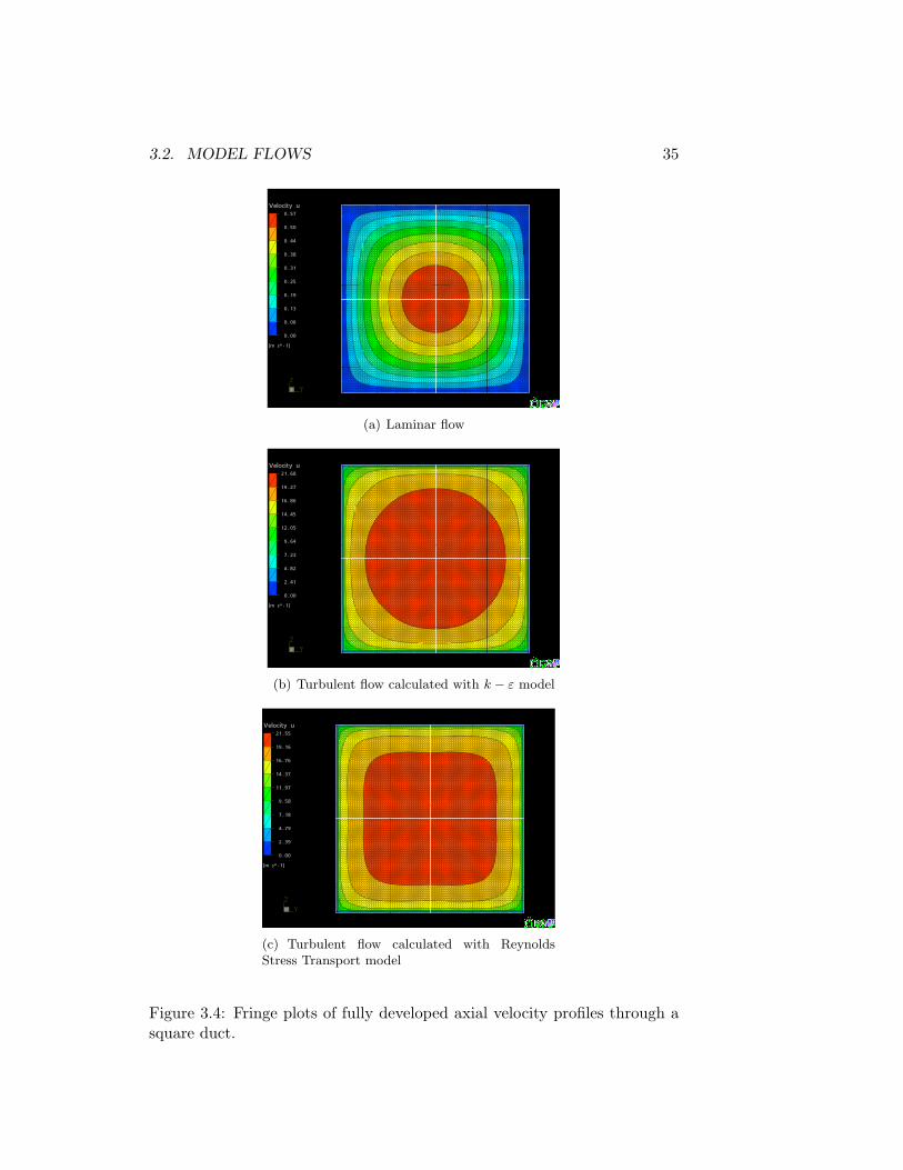
Figure 3.4: From examining the fringe plots of the axial velocity, u, fieldsnotice that:
• For the laminar flow simulation:
– there is a smooth variation of axial speed over the cross-sectional area. The axial speed is maximum at the ductcentre-line (y = z = 0) and is zero at the duct walls y = ±Band z = ±B;
– the iso-vel contours become rounded near the corners indi-cating a zone of relatively slow moving fluid in the cornerregion; and
– the central iso-vel contours are very close to circular in shape.
• For the turbulent flow simulation obtained with the k− ε model:
– there are very large gradients in the axial velocity near theduct walls and the axial velocity is almost uniform over thecentral portion of the duct (the axial speed is within 11% ofthe centre-line value over the central 45% of the duct area).The large gradients near the wall are found in other turbulentflows; and
– the iso-vel contours are again rounded at the corners and thecentral iso-vel contour is very close to circular in shape.
• For the turbulent flow simulation obtained with the ReynoldsStress Transport model:
– there are very large gradients in the axial velocity near thewall and the axial velocity is almost uniform over the centralportion of the duct; however
– the iso-vel contours in the centre of the duct are almostsquare in shape with slightly rounded corners.
3.2. MODEL FLOWS 35
(a) Laminar flow
(b) Turbulent flow calculated with k − ε model
(c) Turbulent flow calculated with ReynoldsStress Transport model
Figure 3.4: Fringe plots of fully developed axial velocity profiles through asquare duct.
36 CHAPTER 3. THE CORNER ATTRACTION
(a) Laminar flow
(b) Turbulent flow calculated with k − ε model
(c) Turbulent flow calculated with ReynoldsStress Transport model
Figure 3.5: Vector plots of cross-stream velocity for fully developed flows inthe upper right quadrant of the square duct.

3.2. MODEL FLOWS 37
(a) Laminar flow
(b) Turbulent flow calculated with k − ε model
(c) Turbulent flow calculated with ReynoldsStress Transport model
Figure 3.6: Fringe plots of x vorticity component for fully developed flowsin the upper right quadrant of the square duct.

38 CHAPTER 3. THE CORNER ATTRACTION
(a) Laminar flow
(b) Turbulent flow calculated with k − ε model
(c) Turbulent flow calculated with ReynoldsStress Transport model
Figure 3.7: Fringe plots of the y normal stress component for fully developedflows in the upper right quadrant of the square duct.

3.2. MODEL FLOWS 39
(a) Laminar flow
(b) Turbulent flow calculated with k − ε model
(c) Turbulent flow calculated with ReynoldsStress Transport model
Figure 3.8: Fringe plots of the z normal stress component for fully developedflows in the upper right quadrant of the square duct.
40 CHAPTER 3. THE CORNER ATTRACTION
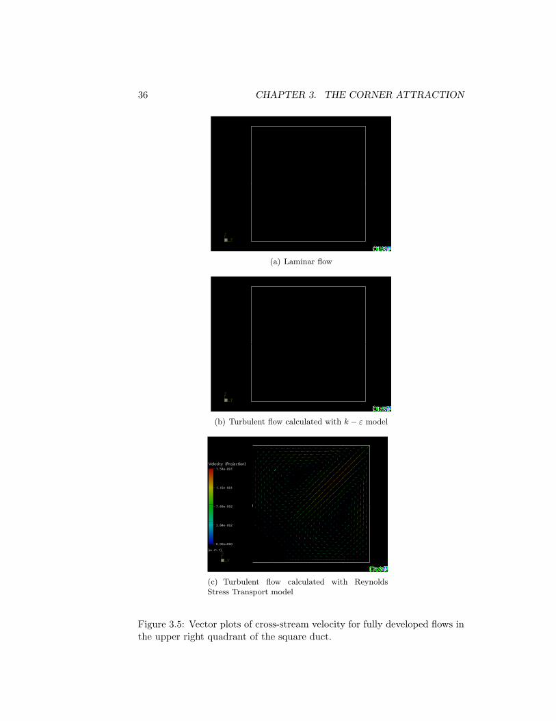
Figure 3.5: The cross-stream velocity is defined as ~Vc−s ≡ vj + wk wherev and w are the velocity components in the y and z directions, re-spectively, and j and k are the unit vectors in the y and z directions,respectively. From examining the cross-stream velocity vector plotsnotice that:
• For the laminar and the turbulent flow simulation obtained withthe k − ε model there is no cross-stream flow, v = w = 0. Theaxial velocity component is the only component in these flows.
• For the turbulent flow simulation obtained with the ReynoldsStress Transport model there is a cross-stream flow with:
– two vortex flows in each quadrant of the square duct;– in each quadrant, the vortex flow is symmetrical about the
radial line running from the duct centre-line to the corner;– the flow along the radial symmetry line is from the duct
centre-line towards the corner;– the centre of the lower vortex is at the non-dimensional lo-
cation yB = 0.76, z
B = 0.41; and– the strength of the simulated secondary flow is weak. The
maximum speed of the cross-stream velocity, ~Vc−s, is 0.7% ofthe centre-line axial velocity.
Figure 3.6: From examining the fringe plots of the x component of thevorticity or the cross-stream vorticity, ζx ≡
(∂w∂y −
∂v∂z
), notice that:
• the cross-stream vorticity or local fluid rotation velocity is onlypresent in the turbulent flow simulated with Reynolds StressTransport model;
• The cross-stream vorticity is anti-symmetrical about the radialsymmetry line in each quadrant of the square duct; and
• the position of greatest cross-stream vorticity is on the upper walland in from the corner a distance of 5% of the duct half-width.
Figures 3.7 and 3.8: From examining the fringe plots of the y and z nor-mal friction stress components, τyy and τzz, notice that:
• for the laminar flow simulation there are no normal friction stresscomponents;
• for the turbulent flow simulation obtained with the k − ε model
3.2. MODEL FLOWS 41
– both τyy and τzz vary from 0.77[Pa] at the duct centreline to2.58[Pa] near the duct walls,
– τyy and τzz stress distributions are symmetrical about theradial symmetry line in each quadrant of the square duct,and
– the normal stress components are also isotropic in that τyy =τzz; and
• for the turbulent flow simulation obtained with the ReynoldsStress Transport model
– τyy varies from 0.67[Pa] at the duct centreline to 1.51[Pa]near the top duct wall,
– τyy is weaker near the right vertical wall than it is near thetop wall,
– τzz varies from 0.67[Pa] at the duct centreline to 1.51[Pa]near the right vertical duct wall,
– τzz is weaker near the top wall than it is near the right verticalwall,
– the τzz distribution in the upper right quadrant is the mirrorimage of the τyy distribution when reflected about the radialsymmetry line,
– the normal stress components are anisotropic in that τyy 6=τzz.
The turbulent flow through the square duct has a set of eight weak butsignificant cross-stream vortices or secondary flows. The secondary flow ineach vortex is drawn from the centreline towards the duct corner along theradial symmetry line. The simulations demonstrate that the existence ofthe secondary flow is connected to the distribution of anisotropic normalstresses, τyy and τzz. How do the anisotropic normal stresses create thesecondary flow?
The simplest explanation of the physics of the secondary flow in a squareduct was proposed by Speziale[17] and is based on the axial vorticity, ζx.The axial vorticity is twice the local counterclockwise (ccw) angular velocityof fluid parcels in the cross-stream or y−z plane. From the definition of theaxial vorticity,
ζx ≡(
∂w
∂y− ∂v
∂z
)(3.1)
it is clear that there will only be axial vorticity if there are velocity com-ponents in the cross-stream plane, v and w. For the fluid parcels to have
42 CHAPTER 3. THE CORNER ATTRACTION
��� ������������ � � ���������
��� ��� �������� �������������
��� ��� ������� ��� ������������
���������������� ��������������
�
�
�! �"����� ���������#!�
�! �"������� �������#$�
�! �%� ���&�����"����#$��! �"����� ����� ����#!�
' '( (
) )* *
+,+-,-
- �%�����������"���#$�
+ �.�����������&���#$�
�! �%�����"��� �����#$� �! �%�����&���������#$�
Figure 3.9: Fluid parcel in a region of high axial vorticity near the right wallwith normal stresses shown on the parcel corners.
angular velocity in the cross-stream plane there must be a moment in thecross-stream plane to create the spin.
Figure 3.9 shows two views of a small fluid parcel, ∆y = ∆z = 0.000625[m],located with its lower left corner at A(y = 0.020[m], z = 0.02375[m]). Asshown in Figure 3.6c, point A lies near the top wall and is in a region ofhigh (ccw) vorticity, ζx = 80[s−1]. The left view of the parcel shows thevalues of the τyy normal stress on the four corners of the parcel and theiraction to create forces and moments on the parcel. The right view showsthe corresponding values of the τzz normal stress.
Consider the τyy normal stresses acting at points B and D. If ∂τyy
∂z
∣∣∣BD
>
0, or τyy|D > τyy|B, then a counterclockwise moment about the parcel’scentre is created on face BD. However, if ∂τyy
∂z
∣∣∣AC
> 0 then a clockwisemoment about the parcel’s centre is created on face AC. The net strengthof the counterclockwise moment on the parcel due to the τyy normal stressis proportional to
∂2τyy
∂y∂z(3.2)
Similarly, there will be a counterclockwise moment created on face CDby the τzz normal stresses if ∂τzz
∂y
∣∣∣CD
< 0. This counterclockwise moment
3.2. MODEL FLOWS 43
will be offset by a clockwise moment on face AB if ∂τzz∂y
∣∣∣AB
< 0. Thereforethe net strength of the counterclockwise moment on the parcel due to theτzz normal stress is proportional to
−∂2τzz
∂y∂z(3.3)
Combining the above shows that a counterclockwise moment about theparcel’s centre is created if
∂2
∂y∂z(τyy − τzz) > 0 (3.4)
In other words, a secondary flow will exist if:
• the normal stresses are anisotropic, τyy 6= τzz, and
• the stress difference, τyy − τzz, varies in both directions in the cross-stream plane, y and z.
����������� ��� ��� �����������
����������� ��� ���������������
��� ������� ��� ������������ ���
������������ ��� ����������� ���
!" "# #
$ $% %
&'&('(
&'&*) �+�,�����-�� ���
&'&*)/. �0�������-��0���112 34 546789:;
11234 546<89:;
&'&>=>) �0�,�����-�� ���(?(>=>)/. �0�,�����-�� �@�
Figure 3.10: Fluid parcel showing the signed normal stress differences oneach face.
Figure 3.10 shows the fluid parcel again with the signed normal stressdifferences on each face along with the moment direction implied by each

44 CHAPTER 3. THE CORNER ATTRACTION
stress difference. Applying a finite difference approximation:
∂2
∂y∂z(τyy − τzz|parcel ≈
(−0.004[Pa] + 0.008[Pa](6.25× 10−4[m])2
)≈ 1.024× 10⁴[Pa/m2]
(3.5)In other words there is a significant positive or counterclockwise moment(per unit volume) acting on the fluid parcel. This moment creates a highcounterclockwise angular velocity or positive vorticity in this region.
3.3 Further Exploration
The secondary flow set up in the cross-stream plane of the square duct isan example of a type two secondary flow. Type one secondary flows aredriven by body forces and include the secondary flow close to a spinningdisk discussed in Chapter 1, The Fate of Sinking Tea Leaves. Type twosecondary flows are driven by normal stresses. For Newtonian fluids, typetwo secondary flows only exist in turbulent flows.
3.3.1 Role of the Turbulence Model
As shown in the original exploration, the simulation of the secondary flowin the square duct is very sensitive to the choice of turbulence model forthe turbulent Reynolds stresses. The eddy viscosity k − ε model failed topredict a secondary flow and the Reynolds stress transport model predictedthe secondary flow to reasonable accuracy. In this sub-section the physics ofthese two turbulence models are briefly reviewed to explain the inadequacyof the eddy viscosity model for this flow. Given the importance of the normalstresses in establishing the vorticity in the cross-stream plane, the focus ison the turbulent normal stress modelling.
The normal stresses, τxx, τyy, τzz are related to the turbulent velocityfluctuations,
ταα = ρu′αu′α (3.6)
where α represents one spatial direction, x, y or z, no summation is implied,and u′α is the turbulent velocity fluctuation in the α direction. The turbulentnormal stresses are also related to the turbulent kinetic energy, k ≡ u′u′
2 +v′v′
2 + w′w′
2 ,τxx + τyy + τzz = 2ρk (3.7)

3.3. FURTHER EXPLORATION 45
The relative sizes of the three normal stresses are determined by how theturbulent kinetic energy is distributed over the three directions.
The eddy viscosity model for the turbulent normal stresses is:
ταα ≈23ρk − 2µT
∂uα
∂xα(3.8)
where µT is the turbulent viscosity (a property of the turbulence). In thefully developed flow through the square duct the streamwise velocity, u, issignificantly larger then the cross-stream velocity and ∂u
∂x ≈ 0. Therefore,eddy viscosity models like the k − ε model predict that all three normalstress components are identical, ταα = 2
3ρk. This normal stress isotropy wasnoted in Figures 3.7 and 3.8.
In Reynolds stress transport models, the transport of the individualstress components is modelled with transport equations of the form:
∂τij
∂t+ Cij = Dij + Pij + Πij − ρεij (3.9)
where Cij is the convective transport of τij ≡ ρu′iu′j by the mean flow field,
Dij is the diffusive transport of τij by the turbulence field, Pij is the shearproduction of τij through products of the shear stresses and mean velocitygradients, Πij is the redistribution of the turbulent kinetic energy betweenthe three directions, and εij is the dissipation of τij by molecular action.The convective transport and shear production terms can be representedexactly in terms of the Reynolds stresses and mean flow gradients. Closuremodels are required for the other three terms.
If the streamwise velocity, u, dominates and the flow is fully developed,∂∂x ≈ 0, then the shear production terms for the three normal stresses are:
Pxx = −2ρu′v′∂u
∂y− 2ρu′w′∂u
∂z(3.10)
Pyy = 0 (3.11)Pzz = 0 (3.12)
This shows that fluctuations in the streamwise direction, u′, are produceddirectly by the mean flow gradients. However, fluctuating velocity compo-nents, v′ and w′, exist in the two cross-stream directions, even though thereis no direct production mechanism for these fluctuations.
The Παα redistribution terms are responsible for creating fluctuationsin the cross-stream directions. There are two redistribution processes: aslow tendency driven by the random motion of the turbulent flow field to

46 CHAPTER 3. THE CORNER ATTRACTION
move towards an isotropic state and a rapid process of cross-stream fluctu-ation creation to conserve mass in the fluctuating velocity field. The latteris pertinent to the study of anisotropy in the square duct flow. When astreamwise fluctuating component is created at a point in space, there mustbe cross-stream fluctuating components created to conserve mass:
∂u′
∂x= −
(∂v′
∂y+
∂w′
∂z
)(3.13)
In regions far from walls, there will be no bias in the creation of v′ andw′ fluctuations. For the simulated flow near the centreline of the ductτyy = τzz = 0.67[Pa] and τxx = 1.37[Pa]. The streamwise normal stressis the highest because of the direct shear production of u′ fluctuations, Pxx.However, approximately half of the kinetic energy produced by this produc-tion is redistributed equally between the v′ and w′ cross-stream fluctuations.
At a point near the top wall, like point A shown in Figure 3.6c, thepresence of the wall will preferentially damp fluctuations in the z direction.In effect, it is easier to pull fluid from the y direction to satisfy the massimbalance created by a shear produced u′ fluctuation then from the z di-rection because of the blockage by the wall. At point A in the simulatedflow, τzz = 1.26[Pa], τyy = 1.43[Pa] > τzz, and τxx = 3.11[Pa]. Again thestreamwise normal stress is the greatest but the redistribution between thev′ and w′ fluctuations is not equal. This is the mechanism that produces theanisotropy in the cross-stream normal stresses that is responsible for creat-ing the secondary flow. An eddy viscosity turbulence model, like the k − εmodel, is not capable of reproducing this anisotropy and therefore cannotreproduce the secondary flow.
3.3.2 Impact of Secondary Flow
As shown in the original explorations, the secondary flow has a profoundeffect on the shape of the streamwise, u, velocity contours even though thestrength of the cross-stream secondary flow is weak. How important is thesecondary flow to the dynamics of the flow through the square duct?
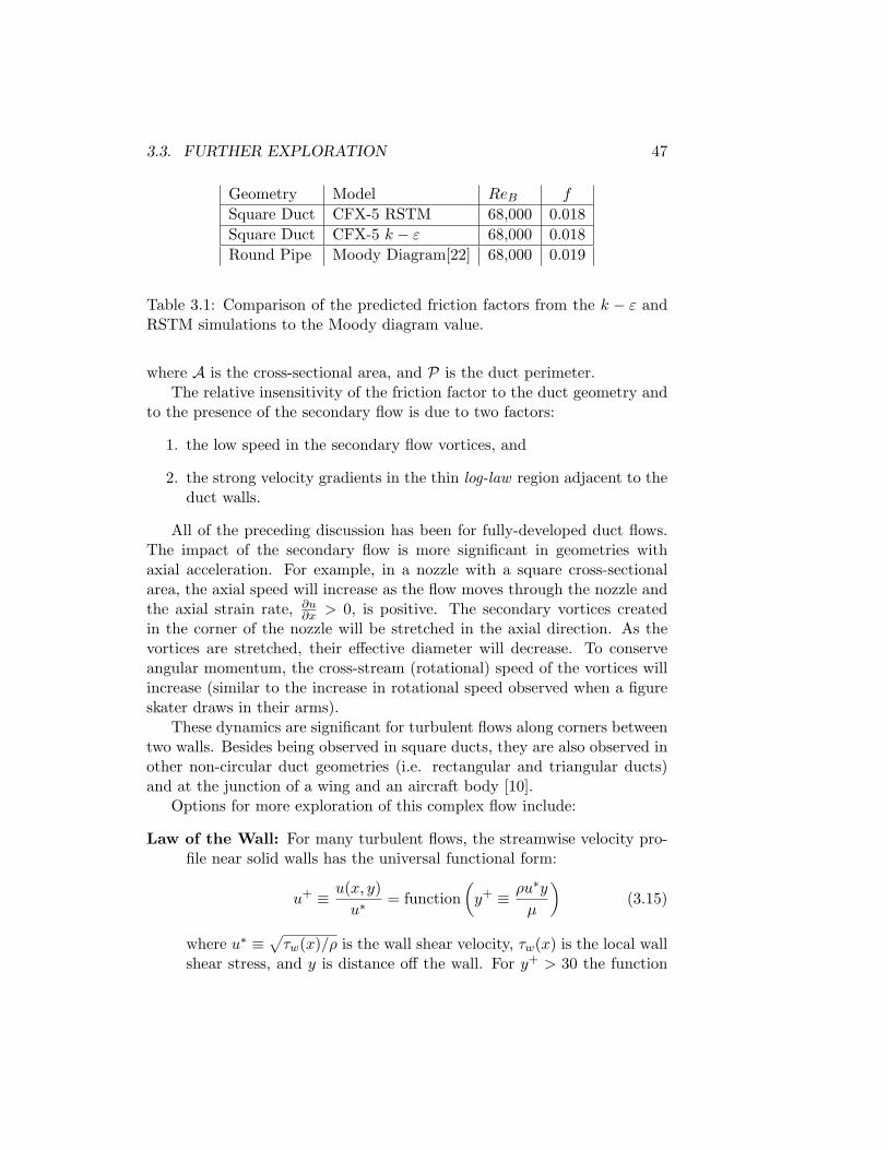
Table 3.1 shows the predicted friction factors from the k−ε and ReynoldsStress Transport Model (RSTM) simulations. This data shows that thesecondary flow does not have any impact on the friction factor. Indeed,the simulated friction factor is very close to that predicted by the Moodydiagram for fully developed flow through a round pipe with a hydraulicdiameter, Dh:
Dh ≡4AP
= 2B (3.14)
3.3. FURTHER EXPLORATION 47
Geometry Model ReB f
Square Duct CFX-5 RSTM 68,000 0.018Square Duct CFX-5 k − ε 68,000 0.018Round Pipe Moody Diagram[22] 68,000 0.019
Table 3.1: Comparison of the predicted friction factors from the k − ε andRSTM simulations to the Moody diagram value.
where A is the cross-sectional area, and P is the duct perimeter.The relative insensitivity of the friction factor to the duct geometry and
to the presence of the secondary flow is due to two factors:
1. the low speed in the secondary flow vortices, and
2. the strong velocity gradients in the thin log-law region adjacent to theduct walls.
All of the preceding discussion has been for fully-developed duct flows.The impact of the secondary flow is more significant in geometries withaxial acceleration. For example, in a nozzle with a square cross-sectionalarea, the axial speed will increase as the flow moves through the nozzle andthe axial strain rate, ∂u
∂x > 0, is positive. The secondary vortices createdin the corner of the nozzle will be stretched in the axial direction. As thevortices are stretched, their effective diameter will decrease. To conserveangular momentum, the cross-stream (rotational) speed of the vortices willincrease (similar to the increase in rotational speed observed when a figureskater draws in their arms).
These dynamics are significant for turbulent flows along corners betweentwo walls. Besides being observed in square ducts, they are also observed inother non-circular duct geometries (i.e. rectangular and triangular ducts)and at the junction of a wing and an aircraft body [10].
Options for more exploration of this complex flow include:
Law of the Wall: For many turbulent flows, the streamwise velocity pro-file near solid walls has the universal functional form:
u+ ≡ u(x, y)u∗
= function(
y+ ≡ ρu∗y
µ
)(3.15)
where u∗ ≡√
τw(x)/ρ is the wall shear velocity, τw(x) is the local wallshear stress, and y is distance off the wall. For y+ > 30 the function

48 CHAPTER 3. THE CORNER ATTRACTION
has a logarithmic form, [21]. Using the data from the simulation offully developed flow through a square duct with a Reynolds StressTransport Model, stored in the spreadsheet SquareDuctData.xls, plotu+ vs y+ on semi-log plots for z = 0, 0.005, 0.01, 0.015, and0.02[m].
Normal Stress Anisotropy: Using the data stored in SquareDuctData.xlscalculate the normal stress anisotropy, v′v′ − w′w′, over the cross-section of the duct 0 < y, z < 0.025[m]. Relate these values to theregions of high vorticity shown in Figure 3.6.
Vortex Production Pettersson Reif and Andersson [14] show that thesecondary flow Reynolds shear stress, v′w′, plays a significant rolein maintaining the secondary flow initially created by normal stressanisotropy. Using the data in SquareDuctData.xls, estimate the vari-ation the secondary vortex production term,
∂2v′w′
∂z2− ∂2v′w′
∂y2(3.16)
over the duct cross-sectional area.
3.3.3 Annotated Reading List
The secondary turbulent corner flow makes an interesting and subtle testbase for understanding the dynamics of turbulent flows. The following isrecommended for further reading:
Johnston[10] Professor Johnston’s article gives a thorough review of thetwo types of secondary flows. Secondary flows in corners are reviewedfor internal duct and external flows.
White[22] Chapter 6 In this introductory text, Professor White intro-duces the concept of hydraulic diameter for the modelling of pressuredrop in non-circular ducts. There is a brief introduction to secondaryflow in the presentation.
Speziale[17] This pioneering article discusses the requirements for a modelof the turbulent Reynolds stresses to successfully capture the sec-ondary flow pattern in rectangular ducts.
Huser and Biringen[9] Presents the findings from an analysis of the com-plete transient turbulent flow field obtained by direct numerical sim-ulation of the transient Navier-Stokes equations for flow in a square
3.3. FURTHER EXPLORATION 49
duct. The transient details of the turbulent eddy motion were resolvedin this simulation.
Pettersson Reif and Andersson[14] Presents a complete analysis of thedynamics of the flow in a square duct based on a simulation obtainedwith a Reynolds Stress Transport Model similar to that used in thepresent work.

50 CHAPTER 3. THE CORNER ATTRACTION
Appendix A
Sinking Tea Leaf Model FlowCalculations
All model flows were calculated using water with nominal properties:, ρ =1000[kg m−3] and µ = 1.0−3[kg m−1s−1]. The outer radius of all containers(and flow domains) was R = 0.025[m].
A.1 1: Spinning Flow Above an Infinite Plate
The simulated flow field of a rotating fluid above an infinite flat plate werecalculated with a semi-analytical procedure. Scale analysis of the full setof momentum equations shows that a the solution can be obtained from aset of non-dimensional ordinary equations. The similarity transformationreduces the radial and axial variation to a variation in a non-dimensionalaxial coordinate, ζ. The derivation and solution of the similarity equationswas first presented by U.T. Boedewadt and is reproduced (with corrections)in Schlichting [16].
A finite volume numerical solution technique was developed for solvingthe similarity equations and was implemented in Matlab 6.0. Full detailsof the derivation of the solution technique are given in a separate report,Stubley [19]. Three Matlab 6.0 script files are available for computing andvisualizing the flow field:
makeprofile.m code to calculate the finite volume solution of the non-dimensional similarity profile functions on a fine mesh. The resultsare written out to a Matlab data file, profile.mat for use in post-processing;
51
52APPENDIX A. SINKING TEA LEAF MODEL FLOW CALCULATIONS
export2tascflow.m code to transform the non-dimensional profile func-tions into dimensional velocity and pressure fields in Cartesian co-ordinates. The results are interpolated onto a CFX-TASCflow meshand exported in an rsf file for visualization processing inside CFX-TASCflow. Note that indirect flow field properties like shear strainrates, stresses, streamlines, etc. are not available; and
plotstreak.m code to transform the non-dimensional profile functions intodimensional velocity and pressure fields in Cartesian coordinates. Thesolution is interpolated onto the coarse mesh and a set of streaklinesare calculated. The resulting plot is animated.
A set of CFX-TASCflow files are also available for visualizing the flowfield:
grd the grid file for a structured mesh of nodes in the x− z plane. Twentyone nodes are placed in the axial direction (H = 0.01[m]) and elevennodes are placed in the radial direction, (R = 0.025[m]). For thebrave of heart, a set of files, gdf, cdf, sdf, and idf, are includedfor generating this mesh with CFX-TASCGrid;
name.lun the CFX-TASCflow system control file;
prm a minimal CFX-TASCflow parameter file;
rso a minimal CFX-TASCflow field data file;
viz.state the information to create the images used in this study; and
rsf the fine grid Matlab 6.0 velocity and pressure field solution interpolatedonto the CFX-TASCflow grid. To use this information restore the post-processing state with viz.state and then use the Command Line Toolto execute the command:”read rsf”.
You may wonder why CFX-TASCflow (or another commercial CFDpackage) was not used to generate the simulated flow field for this modelflow. The boundary conditions for the wall, axis of rotation and far field topare all easily modeled. The boundary condition for the outer cylindrical sur-face is the challenge. The velocity profile over this surface involves regionsof both inflow and outflow and this profile is inherently part of the solu-tion. A well-posed CFD problem requires that the flow field properties beuniquely specified at all inflow regions and that is not possible for this flow.The semi-analytic solution avoids this problem by analytically accountingfor the radial variation and therefore does not require a boundary conditionfor this surface.

A.2. 2: FLOW IN A CONTAINER WITH A SPINNING LID 53
A.2 2: Flow in a Container with a Spinning Lid
A full set of CFX-TASCflow files are provided for this model flow. The meshis generated with CFX-TASCGrid and is made up three meridional planes.The outer two meridional planes define a wedge with an included angle of20◦. A relatively fine mesh with 80 nodes in the axial and radial directionsis used for each meridional plane.
The calculations were done in a rotating reference frame with zero rota-tion rate (this ensures access to post-processing features for rotating flows).The alternate numerics parameter for rotating reference frames was cho-sen to ensure accurate discretization as fluid parcels travel into regions ofvarying bulk rotation about the centre line axis. Water with nominal STPproperties, ρ = 1000[kg m−3] and µ = 1.×10−3[kg m−1s−1] was the workingfluid.
The axis of rotation was modeled as a symmetry line. The bottom andside/outer wall of the container were fixed walls and the lid was a wallboundary with a rotation rate of ω = 0.64[rad s−1].
A second order accurate Linear Profile Skew scheme with Physical Ad-vection Correction (PAC) was used to discretize the advective fluxes. A timestep of 5[s] was used to obtain a steady state solution with the maximumresidual below 1.0× 10⁻⁵.
A macro, torque, is included in the [gci] file for calculating the torque,T [N m], required to turn the spinning lid of the container.
A.3 3: Flow above an Infinite Spinning Plate
MatLab and CFX-TASCflow files similar to those for Model Flow 1 areprovided.
A.4 4: Vortex Breakdown Flow in a Container
The CFX-TASCflow set up for this model flow was identical to that ofModel Flow 2 except that the rotation rate of the spinning lid was ω =2.387[rad s−1] and the height of the container was increased to H = 0.0375[m].The Reynolds number, 1492, and aspect ratio, H/R = 1.5, under these con-ditions were chosen to match the experimental study of Escudier[5].
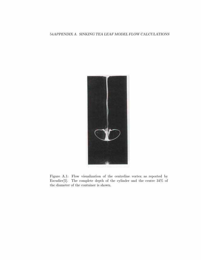
While not shown here, the CFX-TASCflow results are in very good agree-ment with the flow visualizations, Figure A.1, reported by Escudier[5]. Ta-ble A.1 compares the predicted relative position of the stagnation points on
54APPENDIX A. SINKING TEA LEAF MODEL FLOW CALCULATIONS
Figure A.1: Flow visualization of the centreline vortex as reported byEscudier[5]. The complete depth of the cylinder and the centre 34% ofthe diameter of the container is shown.
A.5. 5: TURBULENT FLOW IN A CONTAINER 55
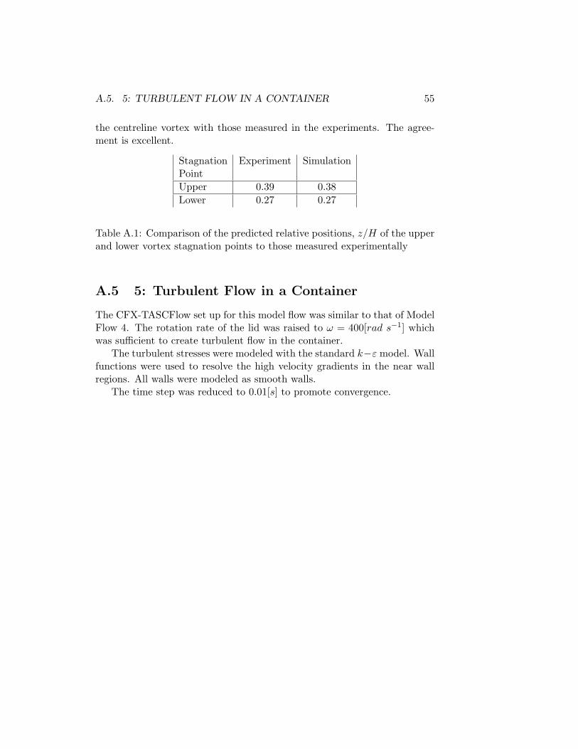
the centreline vortex with those measured in the experiments. The agree-ment is excellent.
Stagnation Experiment SimulationPointUpper 0.39 0.38Lower 0.27 0.27
Table A.1: Comparison of the predicted relative positions, z/H of the upperand lower vortex stagnation points to those measured experimentally
A.5 5: Turbulent Flow in a Container
The CFX-TASCFlow set up for this model flow was similar to that of ModelFlow 4. The rotation rate of the lid was raised to ω = 400[rad s−1] whichwas sufficient to create turbulent flow in the container.
The turbulent stresses were modeled with the standard k−ε model. Wallfunctions were used to resolve the high velocity gradients in the near wallregions. All walls were modeled as smooth walls.
The time step was reduced to 0.01[s] to promote convergence.

56APPENDIX A. SINKING TEA LEAF MODEL FLOW CALCULATIONS

Appendix B
Extra Shock Wave ModelFlow Calculation
This appendix provides the details of the the simulation of the supersonicflow over the wedge airfoil that was performed with CFX-5.4.1. Three caseswere simulated:
Case 1: constant viscosity air flow over no-slip airfoil surfaces,
Case 2: constant viscosity air flow over free slip airfoil surfaces, and
Case 3: temperature dependent viscosity air flow over no-slip airfoil sur-faces.
Figure B.1 shows the two-dimensional geometry that was used for all threecases.
The wedge was 2[mm] long with an included angle of 10◦. The leadingedge of the wedge was placed at the origin of the x − y coordinate system.The solution domain extended 0.5[mm] forward from the leading edge andextended 2.0[mm] back from the trailing edge for a total length of 4.5[mm].The extension of the solution domain back from the trailing edge was re-quired to ensure that approximations in the supersonic outflow boundarycondition, especially in the vicinity of the trailing wake, do not affect accu-racy or convergence. The solution domain extended upwards and downwards2.0[mm] for a total height of 4.0[mm]. This height was sufficient to ensurethat any waves which were reflected off the top and bottom boundaries didnot affect the solution in the region of interest around the leading edge tip.The solution domain had a depth of 0.02[mm]. This thin depth was chosenso that the mesh was one layer of elements deep over most of the solutiondomain.
57
58APPENDIX B. EXTRA SHOCK WAVE MODEL FLOW CALCULATION
Figure B.1: Geometry for the CFX-5 simulation of flow over the supersonicwedge airfoil.
B.1 Physical Models and Boundary Conditions
Air with a temperature of 293.2[K] and a pressure of 101325[Pa] flowedacross the inflow surface shown in Figure B.1 at 673.3[m s−1]. With theseproperties, the Mach number of the flow before the wedge airfoil was 1.965.The air was modelled as a perfect gas with two viscosity models:
1. constant viscosity of 1.785× 10⁻⁵[kg m−1s−1] (Cases 1 and 2), and
2. temperature dependent viscosity (Case 3) based on the Sutherlandcorrelation:
µ(T ) = µ0
(T
T0
) 32 T0 + S0
T + S0(B.1)
where the reference conditions, µO, T0, and S0, are 1.785×10⁻⁵[kg m−1s−1],293.2[K], and 110[K], respectively.
The surfaces of the wedge were modelled as adiabatic surfaces with twofluid flow conditions:
1. no-slip (Cases 1 and 3), or
2. free slip (Case 2).

B.2. MESH 59
The latter was used to simulate inviscid flow over the wedge. The wedgeairfoil was short enough that the boundary layer flow remained as laminarflow so no turbulence model was required.
The front, back, top, and bottom surfaces, shown in Figure B.1, weretreated as symmetric plane surfaces. While this boundary condition causesartificial oblique reflections off the top and bottom surfaces, the reflectedwaves did no affect the flow field over the wedge.
A supersonic outlet boundary condition was applied to the outlet surfaceshown in Figure B.1. This condition allowed all flow properties and waves toleave the solution domain without disturbance. The minimum Mach numberon the outlet surface was 1.58 for Cases 1 and 3 which indicates that theoutlet surface was placed sufficiently far downstream to avoid subsonic flowat the outlet.
B.2 Mesh
An isotropic unstructured mesh of tetrahedral elements was used over thesolution domain. Over most of the solution domain, the average local meshlength was 0.02[mm]. This background mesh length gave approximately 225elements across the width of the domain, 200 elements across the height, and1 element across the depth. The simulations for the inviscid flow over thefree slip surfaces, Case 2, with this background mesh were virtually identicalto those with a mesh length of 0.05[mm], except for the sharpness of theshock waves.
The background mesh length was much too large to resolve the featuresof the laminar boundary flows over the wedge no-slip surfaces. In the im-mediate vicinity of the no-slip surfaces, the mesh length was reduced to0.002[mm] and then gradually expanded by an expansion factor of 1.2 untilreaching the background mesh length. This refined mesh provided approx-imately 15 elements across the width of the laminar boundary layer on thewedge’s bottom surface at 1.0[mm] back from the tip. Since the mesh re-mained isotropic, 750, 000 of the 800, 000 elements in the domain were inthe very thin boundary layer regions. This limited the amount of meshrefinement in the boundary layer region.
B.3 Discretization and Convergence Parameters
Over large regions of the flow domain the flow properties, such as veloc-ity, pressure, and temperature, are uniform. Over isolated shock wave and
60APPENDIX B. EXTRA SHOCK WAVE MODEL FLOW CALCULATION
boundary layer regions, the flow properties change rapidly and are character-ized by large gradients. As discussed above, a fine mesh was used to resolvethe large gradients in the boundary layer regions. Since oblique shock waveshave an almost infinitesimal thickness, a second order discretization schemewas used to ensure that the gradients were adequately resolved over theshock layers. The fringe plots presented in the main body show that sim-ulated shock layers were very thin. While not obvious in the fringe plots,there were slight overshoots and undershoots in some flow properties in theregions of very steep gradients.
A timestep of 1.0×10⁻⁵[s] was used to control the iterative solution. Thistimestep was approximately 1.5 times the advection timescale for fluid tocross the width of the solution domain. With this timestep, approximately60 iterations were required for each case to drive the maximum normalizedresiduals of all equations to below 1.0× 10⁻⁵.
B.4 Computer Results
The calculations were carried out on an Intel I386 architecture computerwith Windows NT4.0 operating system. The following files are available:
airfoil.db : The geometry database used by CFX-Build.
airfoil 001.out : Summary of the CFX-Solver calculations for Case 1.
airfoil 002.out : Summary of the CFX-Solver calculations for Case 2.
airfoil 003.out : Summary of the CFX-Solver calculations for Case 3.
airfoil 001.res : The results files for Case 1.
airfoil 002.res : The results files for Case 2.
airfoil 003.res : The results files for Case 3.
state.cst : A state file for use in CFX-Post for setting up the processingused to generate the fringe plots and spreadsheets.

Appendix C
Corner Attraction ModelFlow Calculation
This appendix provides the details of the simulations of fully-developed flowthrough a square duct that were performed with CFX-5.5.1 (some post-processing was done with CFX-5.6). Three cases involving incompressible airwith nominal properties, density of ρ = 1.284[kg/m3] and dynamic viscosityof µ = 1.725× 10⁻⁵[kg m−1s−1],were simulated:
Case 1: laminar flow with no turbulence model,
Case 2: turbulent flow with the eddy viscosity k−ε turbulence model, and
Case 3: turbulent flow with the SSG form of the Reynolds Stress Transportmodel.
Figure C.1 shows the two-dimensional geometry that was used for allthree cases. The duct had a half-width and half-height of B = 0.025[m].The duct had a depth of 0.0025[m]. This thin depth was chosen so that themesh was only one layer of elements deep in the streamwise direction.
C.1 Physical Models and Boundary Conditions
Because the flow in the square duct is symmetrical about each centre-plane,only the flow in the upper right quadrant was simulated. The leftsym andbotsym surfaces, shown in Figure C.1, are centre-plane surfaces and weretreated as symmetry plane surfaces. The rightwall and topwall surfaces weretreated as smooth wall (no-slip) surfaces.
61

62APPENDIX C. CORNER ATTRACTION MODEL FLOW CALCULATION
�
� �
����������� ������
������������
�!�"�#���$ %�&���
')(+*-, � �
.0/#12*3, � � 465078 *9;:.<.
*-($=>9;:.<.
5<? (@A*CB 5<? (@D*3�
Figure C.1: Geometry for the CFX-5 simulation of fully-developed flow insquare duct.
The flow is fully-developed so all flow properties, except pressure, donot change in the streamwise direction. Therefore, the surfaces inout1 andinout2 were treated as a periodic pair. Since this boundary condition impliesthat all fluid properties, including pressure, are periodic in the streamwisedirection, it was necessary to specify a source term to account for the roleof the streamwise pressure gradient. For fully developed flow in a duct witha hydraulic diameter, 2B, the streamwise momentum source rate per unitvolume, Sx, (due to the streamwise pressure gradient)is
Sx ≡ −∂p
∂x=
2τw
B(C.1)
where τw is the wall shear stress. For a given fluid, the source term can beset to correspond to flow at a nominal Reynolds number based on hydraulicdiameter, ReB ≡ 2ρBu
µ with the friction factor correlation for the wall shearstress:
Sx =2τw
B(C.2)
=ρu2f(ReB)
4B(C.3)
C.2. MESH 63
=ρ
4B
[µReB
2ρB
]2
︸ ︷︷ ︸u2
f(ReB) (C.4)
In the above, u is the cross-sectional average of the streamwise velocity. Thefriction factor correlations for smooth walled square ducts are based on therecommendations of White[22]:
f ≈ 57ReB
ReB < 2000 (C.5)
f ≈[1.8 log10
(6.9ReB
)]−2
4000 < ReB (C.6)
The laminar flow simulations were based on a nominal Reynolds numberof 1000 and the two turbulent flow simulations were based on a nominalReynolds number of 65,000. Note that the actual Reynolds numbers wereslightly different because of differences between the computational modeland the friction factor correlation model.
For the turbulent flow simulations, two turbulence models were used forthe Reynolds stresses:
k − ε Model: The standard form of this eddy viscosity model was used.
Reynolds Stress Transport Model (RSTM): The crucial componentis the model for the redistribution terms, Πij . The standard modelof Rotta was used for the slow return to isotropy and the SSG modelof Speziale et al [18] was used for the rapid process. This latter modelwas selected because of its improved ability to simulate anisotropy inturbulent flows, especially in near wall regions.
For both turbulent models, scalable wall functions were used to resolve thehigh velocity gradients in the near wall regions. The sensitivity of the simu-lated results to the details of the wall boundary conditions are discussed inthe next sub-section.
C.2 Mesh
A mesh with one element depth in the streamwise (periodic) direction wasused. The results presented in the main body, were obtained with a 40element by 40 element square uniform mesh in the cross-stream plane. Thischoice of mesh spacing was based on the results of a grid convergence study.
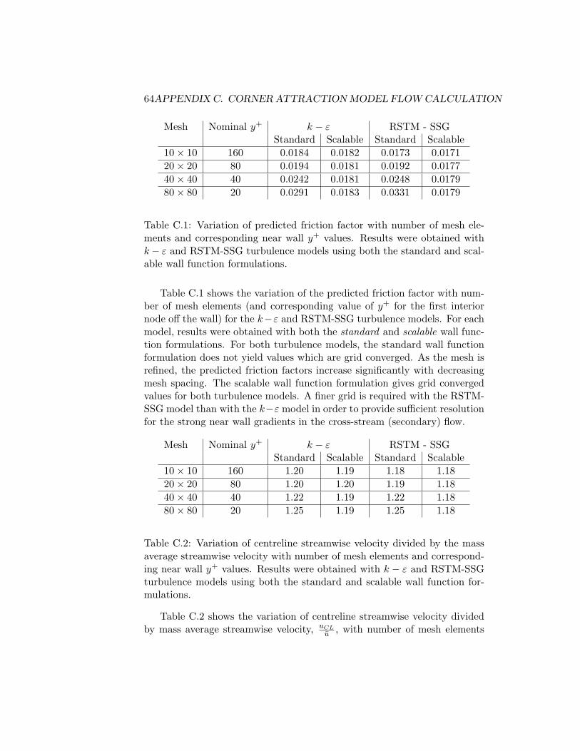
64APPENDIX C. CORNER ATTRACTION MODEL FLOW CALCULATION
Mesh Nominal y+ k − ε RSTM - SSGStandard Scalable Standard Scalable
10× 10 160 0.0184 0.0182 0.0173 0.017120× 20 80 0.0194 0.0181 0.0192 0.017740× 40 40 0.0242 0.0181 0.0248 0.017980× 80 20 0.0291 0.0183 0.0331 0.0179
Table C.1: Variation of predicted friction factor with number of mesh ele-ments and corresponding near wall y+ values. Results were obtained withk− ε and RSTM-SSG turbulence models using both the standard and scal-able wall function formulations.
Table C.1 shows the variation of the predicted friction factor with num-ber of mesh elements (and corresponding value of y+ for the first interiornode off the wall) for the k−ε and RSTM-SSG turbulence models. For eachmodel, results were obtained with both the standard and scalable wall func-tion formulations. For both turbulence models, the standard wall functionformulation does not yield values which are grid converged. As the mesh isrefined, the predicted friction factors increase significantly with decreasingmesh spacing. The scalable wall function formulation gives grid convergedvalues for both turbulence models. A finer grid is required with the RSTM-SSG model than with the k−ε model in order to provide sufficient resolutionfor the strong near wall gradients in the cross-stream (secondary) flow.
Mesh Nominal y+ k − ε RSTM - SSGStandard Scalable Standard Scalable
10× 10 160 1.20 1.19 1.18 1.1820× 20 80 1.20 1.20 1.19 1.1840× 40 40 1.22 1.19 1.22 1.1880× 80 20 1.25 1.19 1.25 1.18
Table C.2: Variation of centreline streamwise velocity divided by the massaverage streamwise velocity with number of mesh elements and correspond-ing near wall y+ values. Results were obtained with k − ε and RSTM-SSGturbulence models using both the standard and scalable wall function for-mulations.
Table C.2 shows the variation of centreline streamwise velocity dividedby mass average streamwise velocity, uCL
u , with number of mesh elements
C.3. DISCRETIZATION AND CONVERGENCE PARAMETERS 65
for the same cases as presented in Table C.1. Again, the results show thatthe standard wall function formulation does not yield grid converged values.The prediction of uCL
u does not show the same sensitivty to grid spacing asobserved above for the friction factor, f .
C.3 Discretization and Convergence Parameters
All simulations for the laminar and turbulent cases were obtained with thesecond order high resolution scheme applied to all transport equations.
Timesteps of 0.5[s] and 1.0× 10⁻³[s] were used for the laminar and tur-bulent flow cases, respectively, to control the iterative solution. With thesetimesteps, approximately 160 iterations and 700 iterations were required forthe laminar and turbulent cases, respectively, to drive the normalized rootmean square(RMS) residuals of all equations to below 1.0 × 10⁻⁶. Whilethe convergence was slow (typical for periodic problems like this where theforcing velocity field is not directly set by the boundary conditions) theconvergence was mostly monotonic.
C.4 Comparison to Experiment and Other Simu-lations
Other experimental and numerical studies of the secondary turbulent flowin a square duct include:
Brundrett and Baines[2] (B&B): Pioneering experimental study of tur-bulent flow in a square duct. Measurements were performed on a flowwith ReB = 83, 000.
Gavrilakis[8] (G): Direct numerical simulation was performed for flow ata ReB = 4, 400.
Huser and Biringen[9] (H&B): Direct numerical simulation was performedfor flow at a ReB = 10, 000.
Pettersson Reif and Andersson[14](P-R&A): A Navier-Stokes solutionbased on the RSTM-SSG model. A high resolution treatment of thenear wall region was used instead of the wall function formulation.Detailed results are presented for flow at a ReB = 10, 000 and frictionfactor results are presented for flow at ReB = 65, 000.

66APPENDIX C. CORNER ATTRACTION MODEL FLOW CALCULATION
Sata et al [15] (S,S,K&T): Particle tracking velocimetry measurementswere made for flow at a ReB = 20, 000.
Geometry Experimenters Model ReB fReB=68,000
Square Duct - CFX-5 RSTM-SSG 68,000 0.018Square Duct - CFX-5 k − ε 68,000 0.018Square Duct P-R& A RSTM-SSG 65,000 0.022Square Duct H& B DNS 10,000 0.021Square Duct B& B Experiment 83,000 0.017Round Pipe Moody[22] Experiment 68,000 0.019
Table C.3: Comparison of friction factors to those measured or predicted byother workers.
Table C.3 shows estimates of the friction factor obtained by various pre-vious workers. Most of the previous work is at Reynolds numbers otherthan 68,000. Reported friction factors have been adjusted to the equivalentfriction factor at a Reynolds number of 68,000 with the Haaland correla-tion [22]:
fReB=68,000 ≈ fmeasured
log(
6.9ReB=measured
)log
(6.9
ReB=68,000
)2
(C.7)
The agreement of the present prediction to previous experimental work inround and square ducts is excellent. The agreement to previous numericalestimates is reasonable given the uncertainty in the turbulence models.
Geometry Experimenters Model ReB
(yV CB , zV C
B
)Square Duct - CFX-5 RSTM-SSG 68,000 (0.78,0.46)Square Duct P-R& A RSTM-SSG 65,000 (0.78,0.46)Square Duct H& B DNS 10,000 (0.82,0.60)Square Duct G DNS 4,400 (0.79,0.50)Square Duct S,S,K&T Experiment 20,000 (0.83,0.44)
Table C.4: Comparison of secondary flow vortex centre position to thosemeasured or predicted by other workers.
The shape of the secondary flow vortex is relatively insensitive to thevalue of Reynolds number at higher Reynolds number,[9]. Table C.4 shows

C.4. COMPARISON TO EXPERIMENT AND OTHER SIMULATIONS67
estimates of the position of the vortex centre,(yV C
B , zV CB
), obtained in various
experimental and numerical studies. The agreement of the present predic-tion to previous work is excellent.
0
0.05
0.1
0.15
0.2
0.25
0.3
0.35
0.4
0.45
0.5
0 0.2 0.4 0.6 0.8 1
Vc−s
u?
y/B
G DNS
3333333333333333333333333333333333333333333333333333333333333333
3S,S,K,&T PTV
++
+++++++++
++++
+++
++
+++++++++
++
++
+
+
+
+CFX 5 - RSTM
2222222222222222222222 222222222222222
2
2
2
2
Figure C.2: Variation of normalized cross-stream flow speed, Vc−s, along thecorner diagonal. Normalization is with respect to the wall shear velocity,u?. The y coordinate is shown in Figure C.1.
When scaled by the wall shear velocity, u? ≡√
τw/ρ, the cross-stream(secondary) velocity field, Vc−s ≡ v(y, z)j + w(y, z)k, is independent of theReynolds number, ReB, [9]. Figure C.2 shows the variation of the nor-malized cross-stream flow along the corner diagonal running from the ductcentreline to the upper right corner. As shown in Figure 3.5c, the max-imum speed of the cross-stream veloicty field occurs along this diagonal.Results are presented from the present study, the Direct Numerical Simu-lation (DNS) of Gavrilakis[8] for a low Reynolds number of 4,400, and forthe experimental study of Sata et al [15] for a Reynolds number of 20,000.The present predictions for the strength of the cross-stream velocity fieldare under-predicted when compared to the experimental findings of Sata etal. This under-prediction can be attributed to the turbulence model and hasbeen noted in other studies that use the Reynolds Stress Transport model,[14]. While the strength of the cross-stream velocity field is under-predicted,

68APPENDIX C. CORNER ATTRACTION MODEL FLOW CALCULATION
the features of the variation along the diagonal, including the near cornerdip and spike, are well predicted.
Overall, the agreement of the present predictions to known experimentalresults and to the numerical studies of previous workers is good.
C.5 Computer Results
The calculations were carried out on an Intel I386 architecture computerwith Windows NT4.0 operating system. The following files are available:
duct laminar.out : Summary of the CFX-Solver calculations for fully-developed laminar flow in a square duct with a 40 × 40 mesh, Case1.
duct ke.out : Summary of the CFX-Solver calculations for fully-developedturbulent flow in a square duct using the k− ε turbulence model on a40× 40 mesh, Case 2.
duct rstm.out : Summary of the CFX-Solver calculations for fully-developedturbulent flow in a square duct using the Reynolds stress transportmodel on a 40× 40 mesh, Case 3.
duct laminar.res The results file for Case 1.
duct ke.res The results file for Case 2.
duct rstm.res The results file for Case 3.
SquareDuctData.xls : Selected mean flow and Reynolds stress fields forCase 3 stored in Microsoft Excel format.

Bibliography
[1] Bardsley, O. and Mair, W.A., 1951, The Interaction between an ObliqueShock-wave and a Turbulent Boundary-layer., Philosophical Magazine,Vol. 42, pp. 29-36.
[2] Brundrett, E. and Baines, W.D., 1964, The Production and Diffusionof Vorticity in a Square Duct, Journal of Fluid Mechanics, Vol. 19, pp.375-394.
[3] Daily, J.W. and Nece, R.E., 1960, Chamber Dimension Effects onInduced Flow and Frictional Resistance of Enclosed Rotating Disks,ASME Journal of Basic Engineering, Vol. 82, pp. 217-232.
[4] Eppler, R., 1990, Airfoil Design and Data, Springer-Verlag, Berlin.
[5] Escudier, M., 1984, Observations of the Flow Produced in a CylindricalContainer By a Rotating Endwall, Experiments in Fluids, Vol. 2, pp.189-196.
[6] Escudier, M., 1987, Confined Vortices in Flow Machinery, Annual Re-view of Fluid Mechanics, Vol. 19, pp. 27-52.
[7] Escudier, M., 1988, Vortex Breakdown: Observations and Explanations,Progress in Aerospace Sciences, pp. 189-229.
[8] Gavrilakis, S., 1992, Numerical Simulation of Low-ReynoldsNUmber Flow Through a Straight Square Duct, Journal ofFluid Mechanics, Vol. 244, pp. 101-129. Data is available athttp://imhefwww.epfl.ch/lmf/research/gavrilakis/homepage.html.
[9] Huser, A. and Biringen, S., 1993, Direct Numerical Simulation of Tur-bulent Flow in a Square Duct, Journal of Fluid Mechanics, Vol. 257,pp. 65-95.
69
70 BIBLIOGRAPHY
[10] Johnston, J.P., 1978, Internal Flows, in Turbulence, Second Correctedand Updated Edition, P.Bradshaw (ed.), Springer Verlag, Berlin, pp.109-169.
[11] Lugt, H.J. and Haussling, H.J, 1973, Development of Flow Circulationin a Rotating Tank, Acta Mechanica, Vol. 18, pp. 255-272.
[12] Lugt, H.J., 1983, Vortex Flows in Nature and Technology, John Wileyand Sons, New York.
[13] Lugt, H.J., 1996, Introduction to Vortex Theory, Vortex Flow Press,Potomac, Maryland.
[14] Pettersson Reif, B.A. and Andersson, H.I., 2002, Prediction ofTurbulence-Generated Secondary Mean Flow in a Square Duct, Flow,Turbulence, and Combustion, Vol. 68, pp. 41-61.
[15] Sata, Y., Sato, K., Kasagi, N., and Takamura, K., 1994, Turbu-lent Air Flow Measurement with Three-Dimensional Particle Track-ing Velocimetry, Transactions of the Japanese Society of Mechan-ical Engineers, Series B, Vol. 60, pp. 865-871. Data available athttp://www.thtlab.t.u-tokyo.ac.jp/PTV/fw rc008.csv.
[16] Schlichting, H., 1979, Boundary-Layer Theory, 7th. Edition, McGraw-Hill, New York.
[17] Speziale, C.G., 1982, On Turbulent Secondary Flow in Pipes of Noncir-cular Cross-Section, International Journal of Engineering Science, Vol.20, pp. 863 - 872.
[18] Speziale, C.G., Sarkar, S., and Gatski, T.B., 1991, Modeling thePressure-Strain Correlation of Turbulence: An Invariant DynamicalSystem Appproach, Journal of Fluid Mechanics, Vol. 227, pp. 245-272.
[19] Stubley,G.D., 2001, Finite Volume Solution of Similarity Equations forRotating Flow over a Fixed Plate, pp. 1-15, Mechanical EngineeringDepartment, Waterloo.
[20] Van Dyke, M., 1982, An Album of Fluid Motion, The Parabolic Press,Stanford, California.
[21] White, F.M., 1991, Viscous Fluid Flow, Second Edition, McGraw-Hill,New York.

BIBLIOGRAPHY 71
[22] White, F.M., 2003, Fluid Mechanics, 5th edition, McGraw-Hill, NewYork.