An Energy-Economy Model to Evaluate the Future Energy Demand-Supply

System in Indonesia

An Energy-Economy Model to Evaluate the Future Energy Demand-Supply

System in Indonesia

The present level of energy demand in Indonesia is still very low and it is expected to continue to increase. To fulfill the demand, some energy resources such as coal,

gas, oil and renewable energy are available. These energy resources are characterized by limited oil reserves, sufficient gas reserves and abundant coal reserves. Therefore, it is important to make optimal strategies for the national energy demand-supply

system for the long future. Energy-economy model is one of the tools for the energy decision maker to perform it. The objective of this study is to develop an energy- economy model for Indonesia

to evaluate the future energy demand-supply systems. Because there is increasing concern about environmental problem recently and for the energy decision maker, the relation among energy, economy and environment become a new consideration, this

model also consider environmental aspect. The model contains five types of primary energy sources: coal, natural gas, crude oil, biomass and other renewable energy which involves hydropower and geothermal

energy. The primary energy sources are transformed into secondary energy sector which consists of electricity and non-electricity. Demand sector is disaggregate into three sectors: industry, transportation and other sectors. The whole country is divided

into four regions: Java, Sumatera, Kalimantan and other islands with transportation of fossil energy: coal, natural gas and crude oil. The model is benchmarked against 1990 base year statistics. The evaluations cover four ten-year time intervals extending from

2000 through 2030. The model is designed as an non-linear optimization model with various components of quantitative framework to make the model useful device for analysis. A software that called General Algebraic Modeling System (GAMS) is used

to solve the problem of the model on 486 compatible personal computer.

According reference case result, abundant coal reserves make coal attractive as the major domestic energy supply in Indonesia. These huge amounts using coal seem to

create high emission of air pollutants. The second major energy supply is natural gas and followed by crude oil. Crude oil supply is expected not growing significantly due to limited of resource.

On the regional perspective, coal is attractive for the energy supply in Java and Sumatera due to the high growth of energy demand in these regions. In Kalimantan natural gas has a significant share for energy supply in a long term. In the other

islands, area is extensive and the energy demands are fewer but much more spread out. Therefore, renewable energy such as hydropower and geothermal energy are attractive in these regions.

Sensitivity analysis is performed by varying the discount rate from 5% to10 % and varying the domestic transportation cost of fossil energy from 50% to 150% of domestic transportation cost of fossil energy in the reference case. At a higher

discount rate, the total income decreases and also the energy demand declines in a long term. A cheaper domestic transportation cost makes increase of the total energy demand. The increasing demand will be supplied by an expansion of coal and natural

gas production. Supply of crude oil will grow if the domestic transportation cost goes up.

0

100

200

300

400

500

600

1990 2000 2010 2020 2030

MTO

E

BiomassHydro&GeoOilGasCoal

Fig. Total primary energy supply projection

Contents List of Figures iii

List of Tables v 1. Introduction 1 2. Background on Indonesia 2

2.1 Geography 2 2.2 Population and economic indicators 2 2.3 Energy 3

3. Background on Energy-Economy Model 7 3.1 Existing energy modeling 7

3.1.1 MARKAL 7

3.1.2 Edmonds-Reilly 8 3.1.3 New Earth 21 9 3.1.4 Global 2100 10

3.1.5 MARIA 14 3.2 Energy technology and resources 15

3.2.1 Crude oil 15

3.2.2 Natural gas 16 3.2.3 Coal 17 3.2.4 Geothermal 17

3.2.5 Hydropower 18 3.2.6 Biomass 19

3.3 Production function 19

3.3.1 Deductive models 20 3.3.2 Inductive models 21 3.3.3 Characteristic 21

3.4 Data analysis 23 4. Model Overview 26

4.1 Energy-economy flow 26

4.2 Mathematical formulation 27 4.3 Population and income data 31 4.4 Sensitivity analysis 31

4.5 The GAMS software 32 5. Result 33

5.1 Aggregate of supply 33

5.2 Regional perspective 35

i

5.3 Emission 37 5.4 Sectoral energy demand 37 5.5 Transportation of fossil fuel 38

5.6 Electricity energy 41 5.7 Sensitivity analysis 41

6. Concluding Remark 44

Acknowledgments 45 References 46 Appendix

A. The GAMS program A-l B. Output of the program B-l

ii

List of Figures 2-1 Indonesia and regional division of the model 2

2-2 Population and GDP growths 3 2-3 Primary energy supply 5 2-4 The commercial energy consumption 5

3-1 Basic energy flows and technology categories 7 3-2 Framework of Edmonds-Reilly model 8 3-3 Projected final energy use 9

3-4 The structure of New Earth 21 model 10 3-5 An overview of ETA-MACRO 11 3-6 Market mechanisms and maximization 11

3-7 Electric energy 13 3-8 Nonelectric energy 14 3-9 Structure of MARIA model 15

3-10 Electricity generation cost 18 4-1 Block diagram of the regionalized model 26 4-2 Structure of regional energy flow model 27

5-1 Population growths 33 5-2 Electricity conversion efficiency 33 5-3 Income growths 34

5-4 Total primary energy supplies 34 5-5 Primary energy supply : Java 35 5-6 Primary energy supply : Sumatera 36

5-7 Primary energy supply : Kalimantan 36 5-8 Primary energy supply : other islands 36 5-9 CO2 emission 37

5-10 Sectoral energy demand 38 5-11 Domestic import of coal 38 5-12 Domestic export of coal 39

5-13 Domestic import of natural gas 39 5-14 Domestic export of natural gas 39 5-15 Domestic import of crude oil 40

5-16 Domestic export of crude oil 40 5-17 Foreign import of crude oil 40 5-18 Electric and nonelectric energy 41

5-19 Total primary energy supply 41

iii

5-20 Import of crude oil 42 5-21 Regional income 42 5-22 Total primary energy supply 42

5-23 Import of crude oil 43 5-24 Regional income 43

iv

List of Tables 2-1 Energy reserves compared to utilization in 1990 4

3-1 Electricity generation technologies 12 3-2 Nonelectric energy supplies 13 3-3 Approximate calorific values of various grades of coal 17

3-4 Historical data 24 3-5 The result of regression analysis 24 3-6 Data and calculation results 25

4-1 The production function parameters 28 4-2 Energy production cost 29 4-3 Energy transportation cost 29

4-4 CO2 release in the production and combustion of fuels 30 4-5 Regional population and income 31

v

1. Introduction The present level of energy demand in Indonesia is still very low and it is expected to continue to increase. To fulfill the demand, some energy resources such as coal, gas, oil and renewable energy are available. These energy resources are characterized by limited oil reserves, sufficient gas reserves and abundant coal reserves. Therefore, it is important to make optimal strategies or planning for the national energy demand-supply system for the long future. The term of energy planning is in wide use now since the fear of energy shortage has emerged after the energy crisis in 1973-1974. Mathematical model has usually been used in energy planning to capture the engineering details of specific energy technology. The energy models can be categorized according to their scope. Its range from supply-oriented models of single fuel to models encompassing the overall energy system coupled to the economy. Four major groups of models can be distinguished: sectoral model, industry market model, energy system model and energy-economy model. The sectoral models defined as relating to some specific energy process or activity forming a part of a specific energy industry market. Typically, the models focus on either the supply or the demand side of the market. Process models are used most often for characterizing energy supply and capacity expansion, whereas econometric models are used to characterize demand. The industry market model include process and econometric model, which characterize both the supply and the demand for a specific of energy products. Such models are very useful and are applicable to all energy-use categories. The modeling in the field of energy system models is very difficult with regard to methodologies and design of models. Generally, simulation and optimization methodologies are applied due to the set of questions addressed by the models. Most of the sectoral and energy system models require that the energy demands must be specified exogenously as input parameters. Most of them create energy demand-supply balances and can be categorized in economic terms as partial equilibrium models. The energy-economy models consist in the coupling of energy system models with models of the overall economy such as macroeconomic and input-output models. This study is modeling in the field of energy-economy models with the object to develop an energy-economy model for Indonesia and to evaluate the future energy demand-supply systems. The whole country is divided into four regions. The model is benchmarked against 1990 base year statistics. Evaluations cover four ten-year time intervals extending from 2000 through 2030. Because there is increasing concern about environmental problem recently and for the energy decision maker, the relation among energy, economy and environment become a new consideration, this model also consider the environmental aspect. The model is designed as an non-linear optimization model with various components of quantitative framework to make the model useful device for analysis.

1

2. Background on Indonesia 2.1 Geography Indonesia, the world's largest archipelago, stretching from 94°45' to 141°5' east longitude and 6°8' north latitude to 11°15' south latitude, is bordered in the west and the south by Indian Ocean. In the east by the Pacific Ocean and in the north by the South China Sea. Indonesia is located in the Southeast Asia, between the Asian Continent in the north, and the Australian Continent in the south. Indonesia extends about 5,150 km from east to west and about 1,770 km from north to south. The Indonesian archipelago consists of no less than 13,700 islands. Around 6,000 islands are inhabited, but only about 3,000 islands have substantial settlements. The total area is about 9.8 million squares kilometers with the sea area is four times larger than its land area (including exclusive economic zone). The land area is generally covered with thick tropical rain forest and predominantly mountainous. The largest islands are Kalimantan (previously known as Borneo) which area of about 539,460 square km, Sumatera with 473,605 square km, Man Jaya (previously called West New Guinea, hording on Papua New Guinea) with 421, 981 square km, Sulawesi (previously called Celebes) with 189,216 square km and Java including Madura, with a land area of about 132,187 square km.

MALAYSIA

Kalimantan

Other Islands

Java

Sumatera

Fig. 2-1. Indonesia and regional divisions of the model 2.2 Population and economic indicators According to the 1990 census the population has reached 179.3 million, which is the third largest group in Asia after People's Republic of China and India. The population growth rate has declined from 2.2% per annum in the early eighties to 1.8% at present due to the success with the family planning program. Compared to other countries, and in particular to industrialized countries, this growth rate is considered very high.

2

The most serious situation is found on Java. The island covers only 7% of the land area but 60% of the Indonesian population lives there. The population density is 842 inhabitants per square km. In the 1970, the country experienced relatively high economic growth of around 7.8% per annum mainly due to the high oil prices in the international market. Average economic growth rate for the last 10 years is about 6% per annum. In early 1983, a series of economic reforms were undertaken to develop and promote exports of agricultural, forestry, and manufacturing that aggregatedly designated as non oil and gas commodities. Strong international competition and the economic momentum of previous achievements prompt Indonesia to broaden industrial base. Indonesia is actively preparing for economic take-off around 1995 with the best chance of success against increasingly global competition.

Fig. 2-2. Population and GDP growths7,11) 2.3 Energy The energy sector is one of the most importance sub-sectors in Indonesia because it has been a major source of technological development, to drive economic activity and also as an export commodity. It accounted for slightly over 20% of GDP in 1990 and approximately 40% of the export earnings. Table 2-1 summarizes the energy resource compared to utilization in 1990. The situation of the fossil energy reserves is characterized by limited oil reserves, sufficient gas reserves and abundant coal reserves. The Indonesia's oil reserves were estimated by Minister of Mine and Energy to be 10.731 billion barrels. Petroleum geologists believed that the not yet explored basins within the Indonesian archipelago contain resources of 30 to 40 billion barrels. The possible oil reserves may be located in remote areas or in the

3

deep sea. High risk exploration and intensive capital investment may be necessary to prove at least part of these resources. The proven and potential gas reserves are estimate at about 101.8×1012 scf. Unfortunately, the most of the reserves have a 70% CO2 content that need large investments to develop the field, to process the gas, and to dispose CO2 into the reservoir.

Table 2-1. Energy reserves compared to utilization in 19908)

Oil 109 Barrel

Natural Gas 1012 scf

Coal 109 ton

Hydropower GW

Geothermal GW

Java 1.325 12.4 0.061 4.2 7.80 Sumatera 8.324 64.1 24.776 15.6 4.90 Kalimantan 1.002 24.4 9.361 21.6 - Other islands 0.080 0.9 0.107 33.6 3.40 Total reserves 10.731 101.8 34.305 75.0 16.10 Production in 1990 0.470 2.1 0.011 - - Installed in 1990 - - - 2.2 0.17

Coal is found predominantly in east and south Kalimantan and central and south Sumatera. The total resources are estimated in 1992 at 34.305 billion tonnes. More than 65% of Indonesian coal is lignite, most is found in south Sumatera. The rest is primarily classified as sub-bituminous and bituminous, although a small amount of anthracite is found in Sumatera. Most of coal reserves have characteristic a low ash, low sulphur and high volatile matter content. Lignites have lower calorific value, higher moisture content and hence higher transportation costs than sub-bituminous, bituminous and anthracite coals. Indonesia has a large hydropower potential of 75 GW. Until 1990, only 2.2 GW was used for electricity generation. Most of the reserves are located in thinly populated areas where the demand is too low to justify large scale investment. The total geothermal has been estimated to be 16 GW. Intensive exploration must be carried out in order to deve lop geothermal reserves. A constraint is also geothermal steam pricing. Therefore, up to now only 140 MW has been used in Kamojang and 220 MW are under development. The domestic primary energy supply in 1991 was accounted around 52 MTOE and was dominated by crude oil with 41% and by biomass, as a traditional form of energy, which contributed 31%. Natural gas supplied 18% of the domestic energy consumption. The remainder was shared by coal (6%) and hydropower together with geothermal energy (4%) as shown in Fig. 2-3. The main consumption of biomass is in the rural and urban peripheral residential sector. Considering the current energy reserves and utilization situation, the general feeling

4

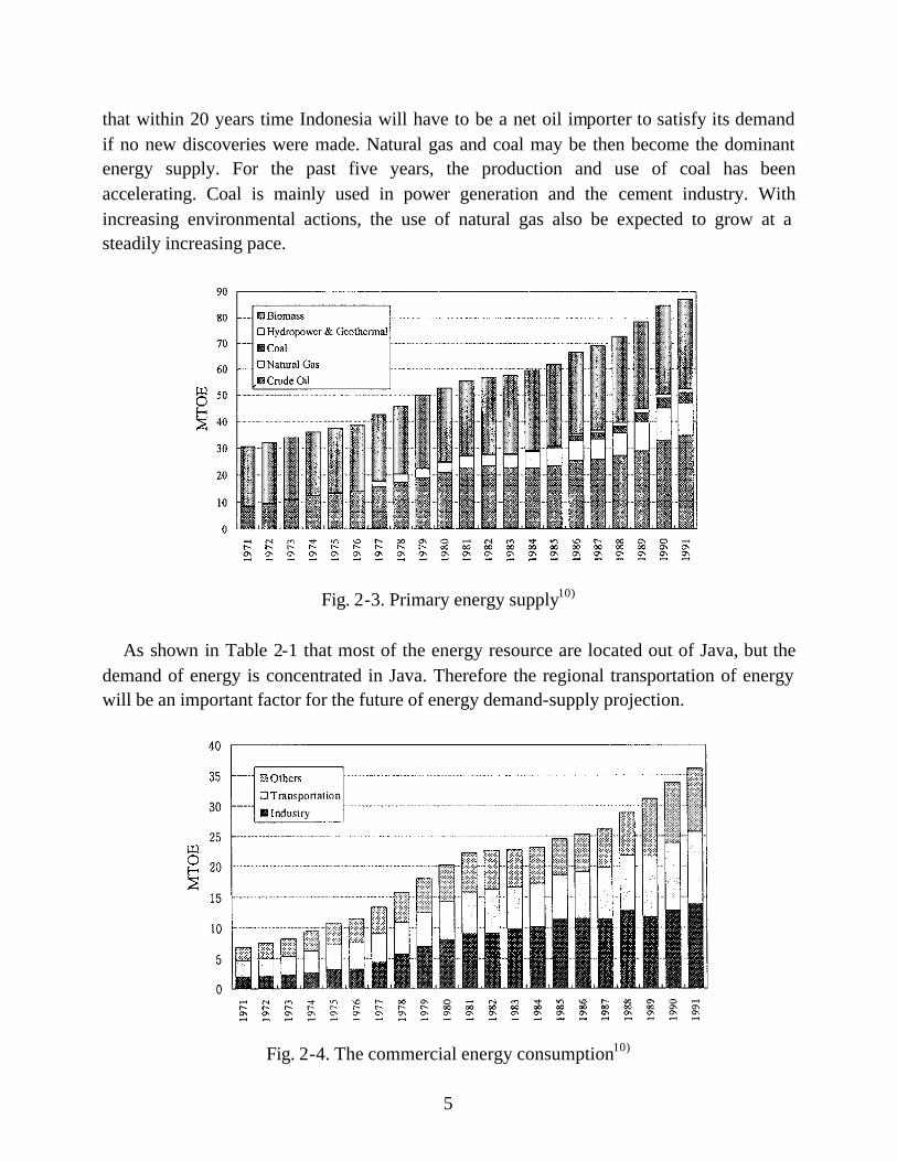
that within 20 years time Indonesia will have to be a net oil importer to satisfy its demand if no new discoveries were made. Natural gas and coal may be then become the dominant energy supply. For the past five years, the production and use of coal has been accelerating. Coal is mainly used in power generation and the cement industry. With increasing environmental actions, the use of natural gas also be expected to grow at a steadily increasing pace.

Fig. 2-3. Primary energy supply10) As shown in Table 2-1 that most of the energy resource are located out of Java, but the demand of energy is concentrated in Java. Therefore the regional transportation of energy will be an important factor for the future of energy demand-supply projection.

Fig. 2-4. The commercial energy consumption10)

5

The present level of energy consumption in Indonesia is still very low and it is expected to continue to increase, as in the most developing countries. An overview of the sectoral commercial energy consumption is given in Fig. 2-4. The industry sector has the highest share of commercial energy consumption. For the last 10 years, the commercial energy consumption in industry sector increased by 3.6%. In transportation sector increased by 5% and the other sectors that includes household, government and commerce sub-sectors, increased by 4.9%.

6

3. Background on Energy-Economy Model

3.1 Existing energy modeling Recently many integrated approaches of energy models, involving interaction among energy, economy, and environmental, has been developed to analysis the future of energy

policy and technology options. Some of the models were described in this section and some of that emphasize on planning of future for mitigating global warming.

3.1.1 MARKAL MARKAL(MARKet ALlocation) was developed in a co-operative effort between Brookhaven National Laboratory (BNL), USA and Nuclear Research Center (KFA),

Germany. About 15 countries belonging to the International Energy Agency (IEA) contributed to the joint effort within the framework of the Energy Technology Systems Analysis Project.

Fig. 3-1 shows the energy flows modeled by MARKAL and the basic categories of technologies are : • resource technologies such as mining, import and export;

• processes which transform energy carrier into one another; • conversion technologies which produce electricity or district heat or both; and • end-use technologies which change some forms of energy into useful services such as

motive power, space heat and transportation.

ResourceTechnologies

End UseTechnologies

Processes

PrimaryEnergy

FinalEnergy

UsefulEnergy

SecondaryEnergy

ConversionTechnologies

Fig. 3-1. Basic energy flows and technology categories14)

MARKAL focuses on the energy sector and linkages to the rest of a nation's economy through the exogenous specification of useful energy demands. Its describes the energy

system by means of a data base and provides software tools which select the variables, constraints, right-hand sides and calculate the numeric values needed. MARKAL is multi-period and linear programming model. Its takes exogenously supplied useful energy

projections and determines the optimal energy supply and end-use network that can meet

7

the demand. An optimal solution is obtained from a collective optimization over the whole set of time periods. The mathematical formulation is shown in equation 3-1, 3-2 and 3-3.

minimize ∑i

ii xc i = 1,…,n (3-1)

subject to ∑ ≤i

jiji bxa j = 1,…,m (3-2)

and 0≥ix (3-3)

The coefficients for the objective function (ci), the coefficients (aji) and the value of right-hand side (bj) are known parameters. The variables (xi) are the unknown quantities to be found. The number of variables is n and the number of constraints is m.

3.1.2 Edmonds-Reilly Edmonds-Reilly model published in 1983 is a global framework for energy assessment

that involves nine global regions. The model can be thought of as consisting of four parts: supply, demand, energy balance and CO2 emissions. The first two modules determine the supply and demand for six major primary energy categories (oil, gas, solids, resource

constrained renewable, nuclear, and solar) in each of regions. The energy balance module assures global equilibrium in each global fuel market and the computations needed to develop projected CO2 emissions. The current terminal analysis date of the model

framework is 2050 with the base year 1975.

Fig. 3-2. Framework of Edmonds-Reilly model12)

8

In this model, supply is determined by a simple extrapolation model. Production of the constrained resource is handled conventionally via a logistics function. The key inputs to

determination of the demand are the level of population, level of economic activity (GNP) and prices of primary energy types. World energy price and demand are determined to meet the world energy supply functions.

Since the program source code of this model is opened for any researcher, it has been modified. Until now it has often provided base case scenarios in many discussions. The base case scenario result of global final energy use by fuel is shown in Fig. 3-3. Among

the four primary fuel categories, electricity production expands most rapidly over the period, averaging nearly 6% per year. Primary solids use grows moderately (3.1% per year), while the use of oil and gas grows more slowly. This is due partly to rising prices of

oil and gas

Fig. 3-3. Projected final energy use13)

3.1.3 New Earth 21

New Earth 21 model was developed by Yasumasa Fujii to evaluate economic and technological feasibility of energy technology combinations with several physical constraints such as supply-demand balances. The whole world is divided into 10 regions

with time horizon from 1990 to 2050 at intervals of 10 years. The principal characteristics of the models is as follows: • Final energy demands will be given exogenously.

• Supply-cost functions of various energy supplies will be given with probabilities of occurrence.

• The model determines the optimum energy-demand pattern, given final demands and

• supply cost functions of energy supplies. The model consists of 10 regional sub-models which optimize the energy flows within the respective regions, and one main-model which manages the interregional energy

9

balances among the sub-models (see Fig. 3-4). The sub-models are linked each other by interregional trade items : natural gas, coal, oil, hydrogen, methanol, ethanol, electricity

and recovered CO2.

Fig. 3-4. The structure of New Earth 21 model23)

The sub-model is formulated as non-linear optimization problem with inequality and/or

equality linear constrains. The constraints represent supply-demand balances and mass-energy balances in various type of energy plants.

• Objective function: Cost for n-th region = Energy system cost in n-th region

+ carbon tax × regional carbon emissions (3-4)

• Subject to:

(3-5)

• Where:

un: the control variables that represented energy supply An: system matrix of n-th region bn: constant (energy demands and existing capacities).

The main model which seeks an equilibrium of the world energy trades is formulated on the basis of the maximum principle of discrete type.

3.1.4 Global 2100

A.S Manne and R.G. Richels developed Global 2100 in 1990. The model is an

extended version of ETA-MACRO model developed in 1970's that linkages between the energy sector and the balance of the economy. This is a merger between ETA (a process model for energy technology assessment) and MACRO (a macroeconomic production

function) that provides for substitution between capital, labor, and energy inputs. ETA-

10

MACRO is a tool for integrating long-term supply and demand projection. Figure 3-5 provides an overview of the principle static linkages of ETA-MACRO. Electric and non-

electric energy are supplied by the energy sector to the rest of the economy. Gross output depends on the inputs of energy, labor and capital. In, turn, output is allocated among current consumption, investment in building up the stock of capital, and current payments

for energy cost.

Fig. 3-5. An overview of ETA-MACRO4)

ETA-MACRO simulates a market or a planned economy over time. There is a single representative producer-consumer. Supplies, demands, and prices are matched through a

dynamic non-linear programming model. A partial equilibrium reasoning applied to a single energy form in a single time period. Consumers' willingness to pay is shown as a smoothly decreasing function of the amount of energy available of them, and producers'

incremental cost are shown as a rising step functions of the amount to be supplied (Fig. 3-6). These functions represent energy demands through a stepwise linear physical process model. Supplies and demands matched through an equilibrium price. It is as though the

economy were attempting to maximize the size of the shaded area (net economic benefits).

Fig. 3-6. Market mechanisms and maximization4)

11

The first version of Global 2100 deals with five major geopolitical regions : the United States, other OECD nations, the Soviet Union, China, and the rest of the world (ROW).

The model is intertemporal with a base year of 1990 and projections cover ten-year time intervals from 2000 through 2100. The national economic activities aggregate into one production function involves various energy technologies.

Table 3-1 identifies the alternative sources of electricity supply. The first five technologies represent existing sources: hydroelectric and other renewables, gas-fired, oil-fired and coal-fired units, and nuclear power plants. The second group of technologies

includes the new electricity generation options that are likely to become available. They differ in terms of their projected costs, carbon emission rates, and dates of introduction.

Table 3-1. Electricity generation technologies4)

Technology name

Earliest possible introduction date

Identification

Existing: HYDRO Hydroelectric, geothermal, and other

renewables GAS-R Remaining initial gas fired

OIL-R Remaining initial oil fired

COAL-R Remaining initial coal fired

NUC-R Remaining initial nuclear

New:

GAS-N 1995 Advanced combined cycle, gas fired

COAL-N 1990 New coal fired

ADV-HC 2010 High-cost carbon free

ADV-LC 2020 Low-cost carbon free

It is expected that new gas-fired capacity for base load electricity will take the form of

combustion turbine combined cycle plants that have a high thermal efficiency, low carbon

emissions, and low capital cost. If natural gas prices remain at their 1990 levels, this technology would represent an attractive source of electricity; however, as natural gas resources gradually become exhausted, fuel prices are likely to rise. With an increase of

this magnitude, gas-fired electricity would lose its competitive advantage over coal. Table 3-2 identifies the nine alternative sources of nonelectric energy. Crude oil price is

crucial to any near or medium-term projections of energy supplies and demands. All other

carbon-based fuels are ranked in ascending order of their cost per GJ of crude oil equivalent. The least expensive domestic source is CLDU that uses in industries such as steel and cement. Next in the merit order are domestic oil and gas.

12

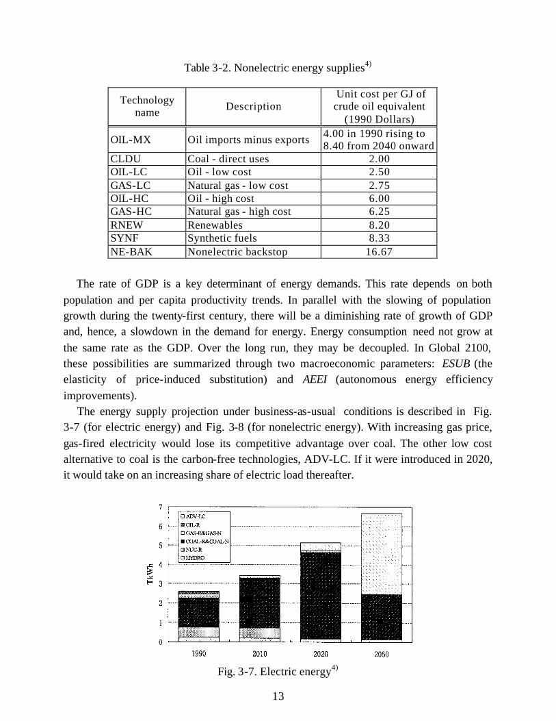
Table 3-2. Nonelectric energy supplies4)

Technology name

Description

Unit cost per GJ of crude oil equivalent

(1990 Dollars)

OIL-MX Oil imports minus exports 4.00 in 1990 rising to 8.40 from 2040 onward

CLDU Coal - direct uses 2.00 OIL-LC Oil - low cost 2.50 GAS-LC Natural gas - low cost 2.75 OIL-HC Oil - high cost 6.00 GAS-HC Natural gas - high cost 6.25 RNEW Renewables 8.20 SYNF Synthetic fuels 8.33 NE-BAK Nonelectric backstop 16.67

The rate of GDP is a key determinant of energy demands. This rate depends on both

population and per capita productivity trends. In parallel with the slowing of population growth during the twenty-first century, there will be a diminishing rate of growth of GDP and, hence, a slowdown in the demand for energy. Energy consumption need not grow at

the same rate as the GDP. Over the long run, they may be decoupled. In Global 2100, these possibilities are summarized through two macroeconomic parameters: ESUB (the elasticity of price-induced substitution) and AEEI (autonomous energy efficiency

improvements). The energy supply projection under business-as-usual conditions is described in Fig.

3-7 (for electric energy) and Fig. 3-8 (for nonelectric energy). With increasing gas price,

gas-fired electricity would lose its competitive advantage over coal. The other low cost alternative to coal is the carbon-free technologies, ADV-LC. If it were introduced in 2020, it would take on an increasing share of electric load thereafter.

Fig. 3-7. Electric energy4)

13

On the nonelectric side, new energy sources become attractive due to increasing crude oil prices. These sources are grouped into two broad categories : SYNF (coal and shale based

synthetic fuels) and RNEW (low-cost carbon-free renewables such as ethanol from biomass)

Fig. 3-8. Nonelectric energy4)

3.1.5 MARIA Multi-regional Approach for Resource and Industry Allocation (MARIA) model, developed by Shunsuke Mori in 1994, is a version of DICE model. W. Nordhaus

developed the DICE model to see the long term interactions between human activities and global warming damages on the world economic growth. Due to the lack of energy flow in DICE model, MARIA model impose energy flows upon the DICE model. This model can

estimate the energy technology options for the long future as well as the international trade prices of fossil fuels and the tradable carbon emission permit under the certain constraints. The model disaggregated primary energy resources into : coal, oil, natural gas,

nuclear, biomass, and other renewable sources which involves hydropower, geothermal and solar energy. Secondary energy sector consists of electric and nonelectric energy. Final consumption sectors are classified into three sectors : industry, transportation and

others. The world is divided into three region : Japan, other OECD countries and others. Figure 3-9 described the structure of MARIA model. The model is a non-linear programming model like Global 2100 model. When a CES type production function is

used in Global 2100 model, this model employs a Cobb-Douglas type production function with capital, labor, electric and nonelectric energy. The model used Negishi-weight in the objective function to guarantee the compatibility between local (national) optimization

behavior and international trade price mechanism. Mathematically, Negishi-weight is given by the inverse of Lagrange multiplier of budget constraint which is proportional to the consumption per capita of each region.

14

Figure. 3-9. Structure of MARIA model19)

3.2 Energy technology and resources24)

The primary energy resources are basically divided into nonrenewable and renewable energy resources. The first group of depletable character includes the fossil energy resource: coal, crude oil and natural gas. The group of renewable resources is base on

geothermal energy, solar energy, hydro power, wind power and biomass. This section only discuss the main characteristic of crude oil, natural gas, coal, geothermal, hydropower and biomass energy that were used in this model.

3.2.1 Crude oil

With the rare exception of being burned directly, the major part of crude oil is

processed into petroleum derivatives. The efficiency of modern petroleum refineries is, in general, around 90% with peak performances. Petroleum refineries consist of crude tankage, a system of separation and conversion process, individual product tanks,

interconnecting lines among the process and tankage, and a system of utilities that provide and distribute the required supply of steam, power, and cooling. Overlying this equipment are process control systems that assure proper flows, temperatures, and pressures; safety

systems that assure the equipment equipment design pressure cannot be exceeded and that discharges are flared in a controlled manner; and environmental system that assure clean refinery effluents.

Crude oil is the feed to refineries. Crudes come in many types, ranging from light crude, which contains higher fractions of gasoline and jet fuel, to heavy crudes containing more heavy oil and asphalt. Sour crudes contain more nitrogen and sulfur compounds than

15

sweet crudes. The objective of a refinery is to manufacture products ranging from the lightest

propane, through gasoline, jet fuels, heating oils, and lumbricating oils to heaviest products, asphalt and coke. The variability in crudes, product characteristic, and demands requires that the equipment be flexible enough to operate over a wide range conditions.

Petroleum products are by far the most versatile and useful energy resources available at present. It is characterized by low costs and ease of transportation. Almost all the needs of the transportation sector and mobile equipment are currently met by petroleum product.

Kerosene and LPG are the favored cooking fuels and the former is the major lighting fuel in area where is no electricity. 3.2.2 Natural gas

Natural gas is a kind of hydrocarbon usually predominantly by methane. They may occur alone (non-associated gas) or in conjunction with crude oil (associated gas).

Production of associated gas dissolved in oil depends on oil production, and is therefore interrupted whenever the latter is shut down for economic or other reasons. Non-associated gas production depend on the structure and characteristics of the reservoir.

Natural gas may contain substantial proportions of non-hydrocarbon gases as impurities. Most of these contain small proportions of heavier hydrocarbons, beside methane, which can readily be reduced to liquid form at the surface by refrigeration or

compression. These so-called wet gases can be processed to produce natural gas liquids (NGL), otherwise know as natural gasoline and liquefied petroleum gases (LPG) consisting of propane and butane.

Historically, crude oil had fundamental advantages over gas as fuel. It could be transported easily and could be processed into petroleum derivatives which could serve different markets. The physical characteristics of natural gas, particularly, difficult to be

transported that make limited its share in the growth of international trade until techniques for ocean transport of liquefied natural gas (LNG) were developed in the 1960s. Hence make natural gas competitive with oil products.

The utilization of gas may also extended to non-traditional uses, such as transport fuels. Compressed natural gas is already being used as a fuel for vehicle in some countries. Methanol, a chemical derivative of natural gas, is eminently suitable for spark plug

engines either as a straight fuel or as an mixture to gasoline. Natural gas can also be converted into gasoline although the cost of conversion is high. Another utilization of natural gas is in fertilizer industry. It is excellent feedstock for nitrogenous fertilizer and a

wide range of basic chemicals. A significant percentage of gas consumption, is represented by these non-energy uses. However, chemical and fertilizer plants themselves are large consumers of energy. Up to 40% of the gas consumed by these installations may

be use as an energy input, rather than as feedstock. 16

If the deposits of natural gas are large and in remote locations, gas production are used exclusively for export in the form of LNG. In this form, however, these resources do not

make any contribution to the energy balances of the producer country. 3.2.3 Coal

The technology for mining, moving and using of coal is well established and steadily improving. Technological advances in combustion, gasification, and liquefaction will greatly widen the scope for the environmentally acceptable use of coal in 1990s and

beyond. The utilization of coal is mainly in industry sector and for the generation of electricity.

The most common classification of coal is calorific content. Hard coal is distinguished

from brown coal and peat, which have less heating values. Within the class of hard coal one can distinguish between steam coal for electric power generation and coking coals, used primary as reductants in steel making. Other important parameters for the

classification of coals are contents of water, volatile matter and ash. This parameters have a large range of variation according to their geological deposit.

Table 3-3. Approximate calorific values of various grades of coal

Grade of coal MJ/kg Hard coal : Steam coal : - Anthracite 33.3 - Bituminous 29.1 - Sub-bituminous 24.7 Coking coal 27.8 Brown coal and lignite 14.7 Peat 8.0

3.2.4 Geothermal

Temperatures in excess of 1000°C exist deep in the earth. The resulting thermal gradient creates a heat flow to the surface which is the source of geothermal energy. Geothermal energy is continuously generated by the flow of heat from the earth's core. It

is, therefore, a renewable form of energy. Geothermal energy can be classified into high level energy and low level energy. The

temperature of geothermal system is normally in the range of 175-315°C, which is

considered low-quality heat by fossil fuel standards. For this reason, the most efficient utilization of geothermal energy would be for the purpose of process heat in industrial applications. But the distance over which the energy can be transported economically is

very limited. By far the largest industrial application of geothermal energy today is the 17

generation of electric power. A pound of steam coming from a man-made boiler fired by conventional fuel is indistinguishable from a pound of steam coming from the earth's

boiler, and the steam turbine does not know the difference. Accepting, then, that electric power can be generated and transported over a transmission system. The electricity generating cost of geothermal energy compare with the other technologies is shown in Fig.

3-10.

Fig. 3-10. Electricity generation cost9)

Exploration for geothermal energy requires a relatively heavy investment in drilling. If the deep drilling does not result in a commercial discovery, the investment will have to be written off as a loss. This is a risk which not all decision makers can take, unless they have

a specific guarantees or insurance, even though the success ratio of geothermal exploration is higher than that of oil exploration.

3.2.5 Hydropower Hydropower technology utilizes the difference of potential energy between different

parts of a water body at a rate which is roughly proportional to the product of water level

difference, commonly refered to as head, and the discharge. Hence, hydropower design and development is directed towards increasing these two quantities both by proper site selection and construction measures.

With regard to the development of head and control of discharge, different plant types can be distinguished: • River power plant, where the head is created by weirs or low dams,

18

• Diversion power plant, which basically utilize naturally available heads, • Run-of-river power plant, which little or no control of discharge, and

• Storage power plant, which high dam and large reservoir for flow regulation. The theoretical annual hydropower potential of a river depends on the precipitation it received annually in its catchment area and the quantity of water remaining on the earth

surface and running down from its altitude to sea level. Since certain portions of the river cannot technically be harnessed, the technical or usable potential, usually, is lower about 50% than the theoretical potential.

3.2.6 Biomass Biomass is a product of photosynthesis due to the capability of the chlorophyll of plants

to absorb the light energy from the sun and to use CO2 of the air for producing sugar and carbohydrates under release of O2 The most important biomass source are: agricultural crop residues, forest residue, animal manures, standing vegetation, aquatic biomass and

solid wasted. Fuel wood, by far the most important biomass from is an important energy especially those living in the rural and urban areas of developing countries. The fuel wood, as a traditional energy is used in residential sector, such as cooking and heating.

There are many technique for advanced utilizing of biomass that convert biomass to useful energy. Generally the process is classified into three category: • Mechanical and thermomechanical process:

o Feedstock preparation o Extraction

• Thermochemical process:

o Direct combustion o Pyrolysis o Gasification

o Liquefaction • Biological process:

o Biomethanation

o Fermentation. 3.3 Production function17)

19

Table 3-4. Historical data7,10,11)

Year Energy Consumption (1000 TOE)

Income (million US dollar)

Population (million)

1971 6736 30.75 122.53 1972 7440 32.72 125.64 1973 8068 35.58 128.80 1974 9322 38.02 132.00 1975 10697 39.95 132.67 1976 11354 42.97 133.53 1977 13266 46.63 136.63 1978 15579 50.13 139.80 1979 17689 52.92 143.04 1980 19996 57.47 147.49 1981 21993 62.25 151.31 1982 22427 62.86 154.66 1983 22666 68.42 158.08 1984 23099 72.69 161.58 1985 24389 74.69 164.63 1986 25084 79.29 168.35 1987 25922 82.91 172.01 1988 28281 88.72 175.59 1989 30337 95.30 179.14 1990 33013 100.40 179.30

(3-14)

The calculation result show in Equation 3-15 and Table 3-5.

(3-15)

Table 3-5. The result of regression analysis

24

Using the parameter α, β and A from regression analysis result, the regional data of income and population in 1990 and using Equation (3-16), the energy-demand regional in

1990 can be calculated as below (i: Java, Sumatra, Kalimantan, and other island).

(3-16)

Table 3-6. Data and calculation results

Region (i) Y (million $) L (million) P (1000 TOE)

Java 60.307 110.359 24738.547 Sumatera 26.719 36.507 10938.564

Kalimantan 5.935 9.100 2431.590

Others 7.448 23.413 3066.685

Total 100.409 179.379 41175.386

From the aggregate data, the total energy demand in 1990 is 33.013 MTOE and from the

regression result the total energy demand in 1990 is 41.175 MTOE that will be acceptable. As shown in Table 3-6 the energy demand in Java is 24.738 MTOE, Sumatera is 10.938 MTOE, Kalimantan is 2.432 MTOE and other island is 3.067 MTOE.

The share of electricity and non-electricity energy in each regions were calculated using the same technique.

25

4. Model Overview

Some of the existing energy-economy models were described in Chapter 3. These techniques are commonly classified into three categories :

• Linear programming model • Simulation of the economy under the assumption of various alternative policies • Computable general equilibrium, such that consumers maximize their utility function.

The last technique is used in this model. 4.1 Energy-Economy flow

The many islands of Indonesia show a significantly non-uniform distribution of energy resource and of energy consumption and a different status of development. Taking this into account, the whole country is divided into four regions: Java, Sumatera, Kalimantan

and other islands (see Fig. 4-1) with transportation of fossil energy: coal, crude oil and natural gas (see Fig. 4-2)

Fig. 4-1. Block diagram of the regionalized model

The real energy flow is represented by a complex network of all relevant energy technologies interconnected by energy carrier from supply side to demand side. In this study an aggregate of energy flow has been used to avoid the complexity of the model.

Each of the region has an energy flow as shown in Fig. 4-2. These individual regions are linked in the model by inter-regional flows such as coal, crude oil and natural gas

26

shipping but is assumed no migration of labor or population.

The model contains five types of primary energy sources: coal, natural gas, crude oil, biomass and other renewable energy which involves hydropower and geothermal energy. The primary energy sources are transformed into secondary energy sector which consists

of electricity and non-electricity. Demand sector is disaggregate into three sectors : industry, transportation and other sectors.

Coal CoalPower Pl ant

Natural Gas GasPower Plant

Coal-Ind.

Coal-Oth.

Gas-Ind.

Gas-Tra.

Gas-Oth.

Oil-Ind.

Oil-Tra.

Oil-Oth.

Electricity

Bi omass fuel

Crude Oil OilPower Plant

Renewable

Biomass

Renew.Power Plant

Preparation

Preparation

Preparation

PreparationTRE_DTRE_F

TRE_DTRE_F

TRE_DTRE_F

I NDUSTRY SECTOR

TRANSPORT SECTOR

OTHER SECTOR

Fig. 4-2. Structure of regional energy flow model

4.2 Mathematical formulation The model is formulated as an intertemporal optimization model with two-way

linkages between the energy sectors and the balance of the economy. The basic formulation to calculate the energy demand is the Cobb-Douglas type production function. Y is the production function in each region r with time period t.

[ ] [ ]ESUBELVSrt

ELVSrt

ESUBKPVSrt

KPVSrtrtrt NELKAY )1(

,,

)1()1(,,,,

−−−= (4-1)

Where E and N denote the production of electricity and non-electricity energy for the industry sector. Unit measurement for the energy production is MTOE. L is a population

assumed as an exogenous variable. K denote capital stock and A is a technical progress factor. The macroeconomics parameters on the above equation are adopted from Global 2100 model4) where ESUB is production value share of energy, KPVS and ELVS are

capital value share parameter and electricity value share parameter.

27

Table 4-1. The production function parameters

Java Sumatera Kalimantan Other

ESUB 0.30 0.12 0.12 0.30 KPVS 0.30 0.30 0.30 0.30

ELVS 0.40 0.40 0.40 0.40

The energy demand in the transportation sector is calculated using equation (4-2). The

supplies of nonelectric and electric energy must be adequate to cover the demands.

)1(

,,,,

,,

αα −≥+ rtrtrtrt

rtrt LYB

EF

EN (4-2)

where α is a value share of income in the transportation sector, EF is the electricity use efficiency and B is a constant. In the other sectors of demand a similar set of energy

demand constraint is employed. The other constraints are the energy resources limit as summarized in Table 2-1. For the fossil energy (coal, natural gas and crude oil) these constraints also calculate the energy transportation to each regions as shown is equation

(4-3).

( ) rt

rtrtrtrt RESFTREDTRENE ≤−−+∑ ,,,, __ (4-3)

where TRE_D and TRE_F are domestic transportation of energy and import of energy. RESr denote the limit of fossil energy resource of region r. The total domestic

transportation of fossil energy must be balanced and is expressed with:

∑ =r

rtDTRE 0_ , (4-4)

In this model, fossil energy resources assume as a static resources with no new discoveries were made along the time horizon. For the biomass energy and other

renewable energy, the resources are renewable in each time period and the production of these energy type are limited by the resources as shown in equation (4-5) and (4-6).

rrt RESRENE ≤, (4-5)

rrt RESBION ≤, (4-6)

28

where RESREN and RESBIO is a other renewable energy resource and biomass energy

resource in each region r. The gross value of production is to be distributed among consumption, investment for build up the capital stock and interindustry payments for energy cost (EC),

rtrtrtrt ECICY ,,,, ++= (4-7)

where C is consumption and I is investment.

Table 4-2. Energy production cost4,18)

US Dollar per TOE

Crude Oil Natural Gas Coal Renewable Biomass

Electricity Nonelectricity

500 105

480 73

550 84

600 -

- 50

The energy cost consists of energy production cost and energy transportation cost. The energy production cost was shown in Table 4-2 and the energy transportation cost was

shown in Table 4-3. Distance from one region to each others is assumed 1000 km. nCTRFFTRECTRDDTRENCSTNECSTEEC rtrtrtrtrt ××+×+×+×= )__( ,,,,, (4-8)

Where ECST and NCST denote electricity and nonelectricity energy production cost, CTRD and CTRF denote domestic transportation cost of fossil energy and energy import cost, n denote time horizon interval.

Table 4-3. Energy transportation cost23)

Transportation Cost $/TOE/1000 km

LNG Natural Gas Pipeline

Oil Coal Electricity line

4.79 19.00

0.67 0.98

170.11

The total capital stock surviving from one period to the next was expressed with:

rtrtrt InKK ,,,1 )1( ×+−=+ δ (4-9)

29

where δ is depreciation rate and n denote time horizon intervals. At the end of the

planning horizon, a terminal constraint is applied to ensure that the rate of investment is adequate.

To avoid excessively rapid expansion of new technologies, there are expansion rate

constraints of the following form. The electricity energy production expansion rate constraint is expressed in equation (4-10) and for the nonelectricity energy in equation (4-11).

rtn

rt EE ,,1 )1( δ−≥+ (4-10)

rtn

rt NN ,,1 )1( δ−≥+ (4-11)

The model maximizes a social welfare function that is the discounted sum of the utility of per capita consumption. In the mathematical formulation can be expressed as:

[ ]∑

−×

××

rt

t

rt

rtrtr d

LC

LS, ,

,, 1logMax (4-12)

where d is the discount rate and C denote consumption. S is share of regional income per capita. In this model depreciation rate and discount rate is set to be 10% and 5% per year. The energy sector, which includes energy production, transport, conversion and end-

use in the sector of industry, transportation and other sectors, is the main contributor to man-made air pollution. The main pollutants are CO2, CO, particulate matter, NOX, SO2, volatile hydrocarbons and some heavy metals.

Table 4-4. CO2 release in the production and combustion of fuels12)

Fuels

Ton Carbon/TOE

Coal Crude Oil Natural Gas Renewable

0.996 0.804 0.574

0

In this study only CO2 emission will be analyse. CO2 emission is associated with the consumption of coal, crude oil, and natural gas. The value for CO2 emission coefficients

for any type of fuels shown in Table 4-4. The CO2 emissions directly estimated if the quantity of each fuel consumed is known. If ECH and NCH are CO2 emission coefficients for fuel use in electricity and nonelectricity then the total CO2 emission is calculated as:

)(2 ,,, NCHNECHECO rtrtrt ×+×= (4-13)

30

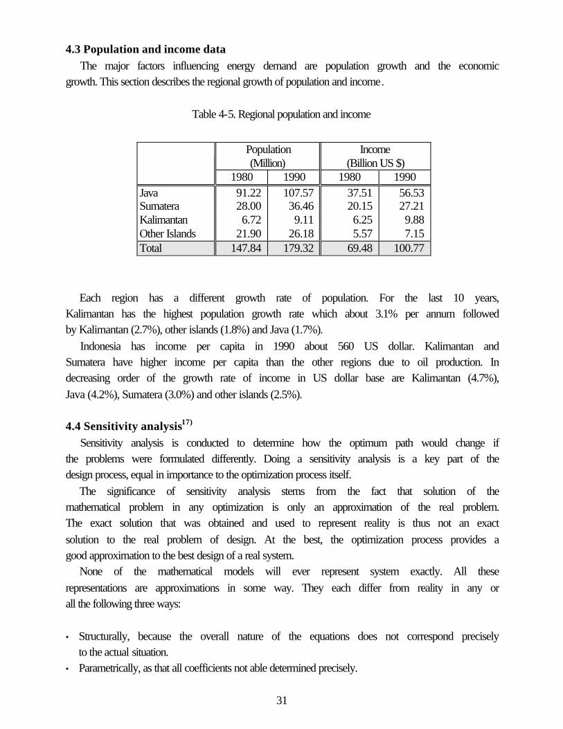
4.3 Population and income data

The major factors influencing energy demand are population growth and the economic growth. This section describes the regional growth of population and income.

Table 4-5. Regional population and income

Population (Million)

Income (Billion US $)

1980 1990 1980 1990 Java 91.22 107.57 37.51 56.53 Sumatera 28.00 36.46 20.15 27.21 Kalimantan 6.72 9.11 6.25 9.88 Other Islands 21.90 26.18 5.57 7.15 Total 147.84 179.32 69.48 100.77

Each region has a different growth rate of population. For the last 10 years, Kalimantan has the highest population growth rate which about 3.1% per annum followed by Kalimantan (2.7%), other islands (1.8%) and Java (1.7%).

Indonesia has income per capita in 1990 about 560 US dollar. Kalimantan and Sumatera have higher income per capita than the other regions due to oil production. In decreasing order of the growth rate of income in US dollar base are Kalimantan (4.7%),

Java (4.2%), Sumatera (3.0%) and other islands (2.5%). 4.4 Sensitivity analysis17)

Sensitivity analysis is conducted to determine how the optimum path would change if the problems were formulated differently. Doing a sensitivity analysis is a key part of the design process, equal in importance to the optimization process itself.

The significance of sensitivity analysis stems from the fact that solution of the mathematical problem in any optimization is only an approximation of the real problem. The exact solution that was obtained and used to represent reality is thus not an exact

solution to the real problem of design. At the best, the optimization process provides a good approximation to the best design of a real system.

None of the mathematical models will ever represent system exactly. All these

representations are approximations in some way. They each differ from reality in any or all the following three ways:

• Structurally, because the overall nature of the equations does not correspond precisely to the actual situation.

• Parametrically, as that all coefficients not able determined precisely.

31

• Probabilistically, in typically assume that the situation is deterministic when it is

generally variable. Structural differences arise as a matter of course in the modeling process. The

mathematical model of a system is typically constructed to imagine some form that believes is appropriate or useful, and then to match the real situation to this structure. The discount rate and the transportation cost of fossil energy are the main parameters

of sensitivity analysis in the model in this study. 4.5 The GAMS software

The model is an non-linear programming model. A software that called General Algebraic Modeling System (GAMS) is used to solve the problem on 486 compatible personal computer. It is generally more difficult to find the solution of non-linear problem

than that of linear one. With non-linear model, it is important to keep the formulation as simple as possible and the model as small as possible. Development of the model should be incremental. Most non-linear problems can be solved more easily if some initial

information is provided for the value of important variables. This can be implemented in the GAMS using initial values, bounds and scaling of variables.

The GAMS1) can solve both linear and nonlinear programming problems. The GAMS

solves linear programming using reliable implementation of the standard simplex method that first developed by G. Danzig in the 1940s. The problem with nonlinear constraints are solved using projected Lagrangean algorithm, base on a method due to S.M.

Robinson. When objective function is nonlinear, GAMS solves such problem using a reduced gradient developed by P. Wolfe in 1962 combined with quasi-Newton algorithm developed by W.C. Davidon in 1959.

32

5. Result

Selected highlights of the model results are presented in this section. This model is run with reference case and sensitivity analysis is performed.

5.1 Aggregate of supply Energy demand-supply grows in line with economic activities and population expansion, In the model population is assumed as an exogenous variable. A continued

decline of the population growth rate is expected because Indonesia family planning policy is attempting to further reduce the growth rate. The total population growth rate until the year 2000 is about 1.8% per annum and 1% per annum for the long term. The

population growths during the whole time horizon until 2030 are presented in Fig. 5-1

0

50

100

150

200

250

300

1990 2000 2010 2020 2030

Mill

ion

Kalimantan OthIsland Sumatera Java

Fig. 5-1. Population growths

0.25

0.275

0.3

0.325

0.35

0.375

0.4

1990 2000 2010 2020 2030

%

Java Sumatera Kalimant OthIsland

Fig. 5-2. Electricity conversion efficiency

33

The other major factors influencing energy demand, addition to population growth and economic growth, are the efficiency with which energy is used. This parameter is also

assumed as an exogenous variable. Fig. 5-2 shows the electricity conversion efficiency projection. The efficiency in Java is higher than the others due to availability of electricity networks in this region.

19902000

20102020

2030

Other Islands

KalimantanSumatera

JavaTotal

0

100

200

300

400

500

600

700

Milli

on 1

990

US

dol

lar

Fig. 5-3. Income growths

With reference case, the income growths are projected and summarized in Fig. 5-3. In

2000 the average annual income growth rate is 5.7 % and 4.6 % until the end of the time horizon. Taking into account the population, in 2000 the income per capita growth rate is 3.9 % per annum. Because the population is still increasing, the income per capita grows

at lower rate of 3.5 % per annum for a long term.

0

100

200

300

400

500

600

1990 2000 2010 2020 2030

MTO

E

BiomassHydro&GeoOilGasCoal

Fig. 5-4. Total primary energy supplies

34

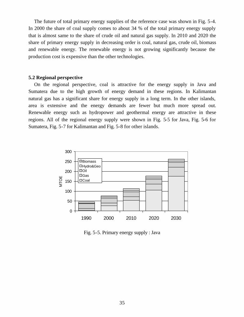
The future of total primary energy supplies of the reference case was shown in Fig. 5-4. In 2000 the share of coal supply comes to about 34 % of the total primary energy supply

that is almost same to the share of crude oil and natural gas supply. In 2010 and 2020 the share of primary energy supply in decreasing order is coal, natural gas, crude oil, biomass and renewable energy. The renewable energy is not growing significantly because the

production cost is expensive than the other technologies.

5.2 Regional perspective On the regional perspective, coal is attractive for the energy supply in Java and Sumatera due to the high growth of energy demand in these regions. In Kalimantan

natural gas has a significant share for energy supply in a long term. In the other islands, area is extensive and the energy demands are fewer but much more spread out. Renewable energy such as hydropower and geothermal energy are attractive in these

regions. All of the regional energy supply were shown in Fig. 5-5 for Java, Fig. 5-6 for Sumatera, Fig. 5-7 for Kalimantan and Fig. 5-8 for other islands.

0

50

100

150

200

250

300

1990 2000 2010 2020 2030

MTO

E

BiomassHydro&GeoOilGasCoal

Fig. 5-5. Primary energy supply : Java

35

02040

6080

100120

140160180

1990 2000 2010 2020 2030

MTO

E

BiomassHydro&GeoOilGasCoal

Fig. 5-6. Primary energy supply : Sumatera

0

10

20

30

40

50

60

70

1990 2000 2010 2020 2030

MTO

E

BiomassHydro&GeoOilGasCoal

Fig. 5-7. Primary energy supply : Kalimantan

0

5

10

15

20

25

30

35

1990 2000 2010 2020 2030

MTO

E

BiomassHydro&GeoOilGasCoal

Fig. 5-8. Primary energy supply : Other islands

36

5.3 Emission Air pollution resulting from coal combustion is probably the most significant

environmental impact associated with the coal fuel cycle and is the topic that generates the greatest amount of international concern. Three main type of emission are involved : sulphur dioxide (SO2), nitrogen oxide (NOX) and paniculate matter.

Increasing used of coal and other fossil energy for the long future in Indonesia seem to create high emission of air pollutions. Therefore, it need to reduce emission in end-use sector (industry, transportation, household) and in power plant using new technology with

low emission rate. For example : in industry sector use the dust control system in the new plants, using electrostatic precipitator and using coal clean technology in power plant. In transportation sector can be use catalytic converters for new car.

0

50

100

150

200

250

300

350

400

450

500

1990 2000 2010 2020 2030

Milli

on T

on o

f Car

bon

OthIsland

Kalimant

Sumatera

Java

Fig. 5-9. CO2 emission

The other emission from energy-used is CO2. Although the CO2 emission in Indonesia is still low comparing with total CO2 emission in the world, Indonesia is aware of this

issue. As one of the 150 signatory states of the Rio Convention, Indonesia agreed to report on the status and tendency of CO2 emission in its territory. The CO2 emission expected by 2030 has been estimated as is shown in Fig. 5-9.

5.4 Sectoral energy demand The energy demand in industry sector, transportation sector and other sectors are

shown in Fig. 5-10. The industry sector has by far the highest energy demand. The growth rate until the year 2030 in industry sector is about 6.7% per annum, in transportation sector is 4.1% per annum and in other sector is 2.0% per annum.

37

0

100

200

300

400

500

600

1990 2000 2010 2020 2030

MTO

E

Other

TransportationIndustry

Fig. 5-10. Sectoral energy demand

5.5 Transportation of fossil energy Domestic transportation and import of fossil energy was shown in Fig. 5-11 to Fig. 5-17. The domestic import means that this region received fossil energy from other regions.

The domestic export means that this region transported fossil energy to other regions. The term of fossil energy import from other countries is indicated by foreign import. Java and other islands received fossil energy from other regions. This energy is

supplied from Sumatera and Kalimantan for coal and natural gas; and from Sumatera only for crude oil. Indonesia will begin import crude oil from other countries in the year 2010 due to the limit of domestic crude oil resources.

19902000

20102020

2030

Sum

ater

a

Kal

iman

tan

Oth

er Is

land

s

Java

0

50

100

150

200

MTO

E

Fig. 5-11. Domestic import of coal

38

1990

2000

2010

2020

2030

Java

Oth

er Is

land

s

Sum

ater

aK

alim

anta

n

0

50

100

150

200

MTO

E

Fig. 5-12. Domestic export of coal

1990

2000

2010

2020

2030

Sum

ater

a

Kal

iman

tan

Oth

er Is

land

sJa

va05

10152025

30

35

MTO

E

Fig. 5-13. Domestic import of natural gas

1990

2000

2010

2020

2030

Java

Oth

er Is

land

s

Kal

iman

tan

Sum

ater

a

0

5

10

15

20

25

MTO

E

Fig. 5-14. Domestic export of natural gas

39

1990

2000

2010

2020

2030

Sum

ater

a

Kal

iman

tan

Oth

er Is

land

sJa

va

0

5

10

15

20

25

MTO

E

Fig. 5-15. Domestic import of crude oil

1990

2000

2010

2020

2030

Java

Oth

er Is

land

s

Kal

iman

tan

Sum

ater

a0

5

10

15

20

25

30

MTO

E

Fig. 5-16. Domestic export of crude oil

1990

2000

2010

2020

2030

Sum

ater

a

Kal

iman

tan

Oth

er Is

land

sJa

va

0

5

10

15

20

25

MTO

E

Fig. 5-17. Foreign import of crude oil

40

5.6 Electric energy Fig. 5-18 summarized the electric energy growths compare to nonelectric energy

growths for the long future. The total energy supply was dominated by nonelectric energy. The growth rate of electric energy is about 5.2% per annum and 4.8% per annum for nonelectric energy.

050

100150200250300350400450500550

1990 2000 2010 2020 2030

MTO

ENonelectric energyElectric energy

Fig. 5-18. Electric and nonelectric energy

5.7 Sensitivity analysis

Sensitivity analysis is performed by varying the discount rate from 5% to 10% and varying the domestic transportation cost of fossil energy from 50% to 150% of domestic transportation of fossil energy in the reference case. The result is shown in Fig. 5-19, Fig.

5-20 and Fig. 5-21 for varying discount rate and Fig. 5-22, Fig. 5-23 and Fig 5-24 for varying domestic transportation cost of fossil energy.

• Discount rate At a higher discount rate, the total income decreases and also the energy demand declines in a long term. The import of crude oil from other countries will be delayed from the year

2010 to 2020 at a higher discount rate.

0

100

200

300

400

500

600

'5%' '7.5%' '10%'

MTO

E

BiomassHydro&GeoOilGasCoal

Fig. 5-19. Total primary energy supply

41

0

10

20

30

40

50

60

'5%' '7.5%' '10%'

MTO

E

2030202020102000

Fig. 5-20. Import of crude oil

0

100

200

300

400

500

600

700

800

'5%' '7.5%' '10%'

Milli

on 1

990

US

dol

lar

Other Islands

SumateraKalimantan

Java

Fig. 5-21. Regional income

• Domestic transportation cost

A cheaper domestic transportation cost makes increase of the total energy demand. The increasing demand will be supplied by an expansion of coal and natural gas production. Supply of crude oil will grow if the domestic transportation cost of fossil energy goes up.

0

100

200

300

400

500

600

700

'50%' 'Ref' '150%'

MTO

E

BiomassHydro&GeoOilGasCoal

Fig. 5-22. Total primary energy supply

42

0

10

20

30

40

50

60

'50%' 'Ref' '150%'

MTO

E

2030202020102000

Fig. 5-23. Import of crude oil

0

100

200

300

400

500

600

700

800

'50%' 'Ref' '150%'

Milli

on 1

990

US

dol

lar

Other IslandsSumatera

KalimantanJava

Fig. 5-24. Regional income

43

6. Concluding remarks

Abundant coal reserves make coal attractive as the major domestic energy supply in Indonesia. These huge amounts using coal seem to create high emission of air pollutants.

The second major energy supply is natural gas and followed by crude oil. Crude oil supply is expected not growing significantly due to limited of resource.

On the regional perspective and a long term, in Java and Sumatera the energy supply is

dominated by coal. In Kalimantan, however is dominated by natural gas. Renewable energy such as hydropower and geothermal energy are attractive in other islands.

Doing sensitivity analysis shows the total income and energy demand will decline at a

higher discount rate. A cheaper domestic transportation cost make increasing the energy demand and it supplied by an expansion of coal and natural gas production. Supply of crude oil will grow if the domestic transportation cost goes up.

When one considers the increasing of electricity consumption, it would be desirable to extent this model with electricity energy transportation to the other regions, such as using submarine cable from Sumatera, that abundant of fossil fuel, to Java that shows rapidly

increase of energy demand in the future study.

44

Acknowledgments I particularly thanks to Professor Dr. Shunsuke Mori for guidance and advice. I also thanks to Dr. Harada Taku for valuable discussion and to all Mori-Laboratory members,

who helped while I have been living in Japan. I am much indebted to Professor. Dr. Yoichi Kaya and all members of Kaya-Hori Laboratory, who helped when I studied at Tokyo University.

45

References [1] A. Brooke, D. Kendrick and A. Meeraus, Release 2.25 GAMS User's Guide, The

Scientific Press, 1992.

[2] Agus Sugiyono and Shunsuke Mori, Integrated Energy System to Improve Environmental Quality in Indonesia, , p.71-74, SICE, October, 1994.

[3] Agus Sugiyono and Shunsuke Mori, Energy-Economy Model to Evaluate the Future Energy Demand-Supply in Indonesia, , p.365-370, 1995.

[4] Alan S. Manne and Richard G. Richels, Buying Greenhouse Insurance: The economic costs of CO2 emission limit, The MIT Press, 1992.

[5] Andy S. Kydes, Flow Models, Energy-The International Journal, Vol. 15, No. 7/8,

p.561-571, 1990. [6] A. Reuter and A. Voss, Tools for Energy Planning in Developing Countries,

Energy-The International Journal, Vol. 15, No. 7/8, p.705-714,1990.

[7] Asian Development Bank, Key Indicators on Developing Asian and Pacific Countries, Vol.XXIII, 1992.

[8] BPPT-KFA, Environmental Impact of Energy Strategies for Indonesia: Final Summary Report, May 1993.

[9] Carel Otte, Geothermal Energy Opportunities for Developing Countries, Proceeding of the Energy and the Environment in the 21st Century Conference, The MIT Press,

p.755-761,1991 [10] International Energy Agency, The IEA Energy Balance and Statistics Databases, on

diskette ,1993.

[11] International Monetary Fund, International Financial Statistics Yearbook, Publication Services IMF, Washington, 1993.

[12] Jae Edmonds and John Reilly, A long-term global energy-economic model of carbon dioxide release from fossil fuel use, Energy Economics, p.74-88, April 1983.

[13] Jae Edmonds and John Reilly, Global Energy Production and Use to the Year 2050, Energy -The International Journal, Vol. 8, No. 6, p.419-432, 1983.

[14] Manfred Kleemann and Dieter Wilde, Intertemporal Capacity Expansion Models, Energy-The International Journal, Vol. 15, No. 7/8, p.549-560,1990.

[15] Oleg A. Eismont, Long-term macroeconomic estimate of energy consumption,

Energy Economic, Vol. 14, No. 4, p.271-273, October 1992. [16] R.G.D. Alien, Macro-Economic Theory: A Mathematical Treatment, St. Martin's

Press, 1968.

[17] Richard de Neufville, Applied System Analysis, McGraw-Hill, 1990.

46

[18] Shunsuke Mori, A Long Term Evaluation of Nuclear Power Technology by DICE+e Model Simulations, International Symposium on Global Environment and Nuclear Energy Systems, Japan, October 1994.

[19] Shunsuke Mori, MARIA - Multi-regional Approach for Resource and Industry Allocation model - and its First Simulations, Technical report, Department of Industrial Administration, Science University of Tokyo, October 1994.

[20] United Nations, Statistical Yearbook, 1993.

[21] William a. Buehring, Energy and Economy Modeling on the Microcomputer, Energy-The International Journal, Vol. 15, No. 7/8, p.697-704,1990.

[22] World Energy Council, Energy for Tomorrow's World, St. Martin's Press, 1993.

[23] Yasumasa Fujii, Energy System for Mitigating and Evaluation of CO2 Emission Problem, in Japanese, Ph.D. Dissertation, Tokyo University, Tokyo, 1993.

[24] M. Kleemann, B. Romahn and D. Wilde, Energy and Energy R&D Strategies for Indonesia: Training Program Manual, KFA, 26th September – 9th December 1983.

47

APPENDIX A

GAMS SOURCE PROGRAM

A-1

* An Energy-Economy Model to Evaluate the Future Energy Demand-Supply System* in Indonesia* Author : Agus Sugiyono* January 1995

$OFFSYMXREF OFFSYMLIST OFFUELLIST OFFUELXREFFILE FSAVE /EEBAS.OUT/;PUT FSAVE;PUT "* BASE CASE *" /;

SETS T Time period /1990, 2000, 2010, 2020, 2030/ TFIRST(T) First period TLAST(T) Last period RG Region /JAV, SMT, KAL, OTH/ ITR Iteration /1*3/

AT All Technology /COA-I Coal to Industry Sector COA-O Coal to Other Sector GAS-I Gas to Industry Sector GAS-T Gas to Transportation Sector GAS-O Gas to Other Sector OIL-I Oil to Industry Sector OIL-T Oil to Transportation Sector OIL-O Oil to Other Sector BIO-O Biomass Fuel to Other Sector COA-P Electric from Coal GAS-P Electric from Gas OIL-P Electric from Crude Oil HYDRO Electric from Hydropower GEOTR Electric from Geothermal /

ET(AT) Electricity Technology /COA-P, GAS-P, OIL-P, HYDRO, GEOTR/

NT(AT) Nonelectric Technology /COA-I, COA-O, GAS-I, GAS-T, GAS-O, OIL-I, OIL-T, OIL-O, BIO-O/

TCOA(AT) Coal Base Technology /COA-I, COA-O, COA-P/ TGAS(AT) Gas Base Technology /GAS-I, GAS-T, GAS-O, OIL-P/ TOIL(AT) Oil Base Technology /OIL-I, OIL-T, OIL-O, GAS-P/

FOSS Fossil fuel for regional transportation /COAL, NGAS, COIL/

EDM Electricity Sectoral Demand /ELE-I, ELE-T, ELE-O/

NIND(AT) Nonelectricity in Industry Sector /COA-I, GAS-I, OIL-I/ NTRA(AT) Nonelectricity in Transportation Sector /GAS-T, OIL-T/ NOTH(AT) Nonelectricity in Other Sector /COA-O, GAS-O, OIL-O, BIO-O/

SCALARS NYPER Number of years per period /10./ BET Discount factor /0.95/ DK Depreciation rate on capital per year /0.10/

A-2

A0 Initial level of total factor productivity /1.0/ GA0 Initial growth rate for technology per decade /0.25/ DELA Decline rate of technology change per decade /0.08/

PFPF Proportional factor of production function /0.10/ PFEC Proportional factor of energy cost /6500/ PFFC Proportional factor of foreign transp. cost /900/ PFDC Proportional factor of domestic transp. cost /90/

PARAMETERS R(RG) Rate of social time preference per year /JAV .025 SMT .020 KAL .020 OTH .025/

K0(RG) Initial capital (Billion 1990 US dollar) /JAV 107.86 SMT 86.74 KAL 29.52 OTH 25.75/

I0(RG) Initial investment (Billion 1990 US dollar) /JAV 23.477 SMT 10.402 KAL 2.306 OTH 2.900/

C0(RG) Initial consumption (Billion 1990 US dollar) /JAV 5.729 SMT 2.539 KAL 0.563 OTH 0.708/

N0(RG) Initial nonelectric energy E0(RG) Initial electric energy L0(RG) Initial population

Y0(RG) Initial productivity (Billion 1990 US dollar) /JAV 56.53 SMT 27.21 KAL 9.88 OTH 7.15/

ESUB(RG) Production value share of energy /JAV 0.30 SMT 0.12 KAL 0.12 OTH 0.30/

KPVS(RG) Capital value share /JAV 0.30 SMT 0.30 KAL 0.30 OTH 0.30/

ELVS(RG) Elasticity of electricity in industry /JAV 0.40 SMT 0.40 KAL 0.40 OTH 0.40/

A(RG) Output scaling factor

RESBIO(RG) Limit of biomass use per annum (MTOE)

A-3

/JAV 10.0 SMT 14.0 KAL 15.0 OTH 8.0/

RESGEO(RG) Limit of geothermal use per annum (MTOE) /JAV 4.113 SMT 2.585 KAL 0.001 OTH 1.792/

RESHYD(RG) Limit of hydropower use per annum (MTOE) /JAV 2.215 SMT 8.226 KAL 11.390 OTH 17.718/

EATRN(RG) Income elasticity in transportation sector /JAV 0.403 SMT 0.403 KAL 0.403 OTH 0.403/

EAPUB(RG) Income elasticity in others sector /JAV 0.312 SMT 0.312 KAL 0.312 OTH 0.312/

EFF0(RG) Final electric conversion efficiency /JAV 3.0 SMT 2.8 KAL 2.7 OTH 2.3/

EFFA(RG) Constant term of electric conversion eff. /JAV 7.3333 SMT 7.3333 KAL 7.3333 OTH 7.3333/

EFFB(RG) Time dependence term of electric conversion eff. /JAV -0.003 SMT -0.003 KAL -0.003 OTH -0.003/

GL0(RG) Population after 2100 /JAV 161 SMT 103 KAL 27 OTH 75/

GLA(RG) Constant term of population /JAV 0.490 SMT 1.788 KAL 1.788 OTH 1.788/

GLB(RG) Time dependence term of population /JAV -0.056 SMT -0.037 KAL -0.049 OTH -0.025/

A-4

CH(AT) Carbon Emission Coefficient (Ton Carbon per TOE) /COA-I 1.000 COA-O 1.000 GAS-I 0.578 GAS-T 0.578 GAS-O 0.578 OIL-I 0.825 OIL-T 0.825 OIL-O 0.825 BIO-O 0.000 COA-P 1.000 GAS-P 0.578 OIL-P 0.825 HYDRO 0.000 GEOTR 0.000/

BETA(T) Annual discount factor AL(T) Technical progress L(T,RG) Level of population (Million) EFF(T,RG) Electric power conversion efficiency DKT Depreciation rate per decade SHARE Income per capita in 1990 NEGISHI(RG) Share of income percapita ;

TABLE RESF(FOSS,RG) Resource of fossil fuel (MTOE) JAV SMT KAL OTH COAL 39 15762 5955 68 NGAS 306 1580 601 22 COIL 185 1161 140 11 ;

TABLE ECST(ET,RG) Electricity cost coefficient (Dollar per TOE) JAV SMT KAL OTH COA-P 550.000 550.000 550.000 550.000 GAS-P 480.000 480.000 480.000 480.000 OIL-P 500.000 500.000 500.000 500.000 HYDRO 600.000 600.000 600.000 600.000 GEOTR 580.000 580.000 580.000 580.000 ;

TABLE NCST(NT,RG) Nonelectric cost coefficient (Dollar per TOE) JAV SMT KAL OTH COA-I 83.720 83.720 83.720 83.720 COA-O 83.720 83.720 83.720 83.720 GAS-I 62.790 62.790 62.790 62.790 GAS-T 62.790 62.790 62.790 62.790 GAS-O 62.790 62.790 62.790 62.790 OIL-I 104.650 104.650 104.650 104.650 OIL-T 104.650 104.650 104.650 104.650 OIL-O 104.650 104.650 104.650 104.650 BIO-O 60.000 60.000 60.000 60.000 ;

TABLE CTRD(FOSS,RG) Domestic transport. cost of fossil (Dollar per TOE) JAV SMT KAL OTH COAL 0.980 0.980 0.980 0.980 NGAS 4.790 4.790 4.790 4.790 COIL 0.670 0.670 0.670 0.670 ;

TABLE CTRF(FOSS,RG) Foregin transport. cost of fossil (dollar per TOE) JAV SMT KAL OTH COAL 1.960 1.960 1.960 1.960 NGAS 9.580 9.580 9.580 9.580

A-5

COIL 1.340 1.340 1.340 1.340 ;

TABLE PRO0(AT,RG) Energy production in 1990 (MTOE) JAV SMT KAL OTH COA-I 2.442 0.422 0.015 0.022 COA-O 0.132 0.011 0.002 0.002 GAS-I 3.852 0.942 0.542 0.582 GAS-T 0.404 0.017 0.002 0.005 GAS-O 2.604 1.102 0.002 0.003 OIL-I 8.455 3.342 1.142 1.152 OIL-T 8.708 2.570 1.073 1.782 OIL-O 6.876 2.642 0.452 0.402 BIO-O 7.130 6.342 1.642 1.924 COA-P 0.612 0.322 0.107 0.112 GAS-P 0.173 0.031 0.023 0.031 OIL-P 2.708 0.712 0.409 0.442 HYDRO 0.678 0.335 0.137 0.142 GEOTR 0.868 0.012 0.001 0.022 ;

TABLE DMD0(EDM,RG) Lower bound of electricity energy (MTOE) JAV SMT KAL OTH ELE-I 0.792 0.154 0.015 0.103 ELE-T 0.005 0.000 0.000 0.000 ELE-O 0.672 0.125 0.015 0.103 ;

TABLE IMD0(FOSS,RG) Lower bound of domestic import of fossil (MTOE) JAV SMT KAL OTH COAL 0.000 0.000 0.000 0.000 NGAS 0.000 0.000 0.000 0.000 COIL 0.000 0.000 0.000 0.000 ;

TABLE EXD0(FOSS,RG) Lower bound of domestic export of fossil (MTOE) JAV SMT KAL OTH COAL 0.000 0.000 0.000 0.000 NGAS 0.000 0.000 0.000 0.000 COIL 0.000 0.000 0.000 0.000 ;

TABLE IMF0(FOSS,RG) Lower bound of foreign import of fossil (MTOE) JAV SMT KAL OTH COAL 0.000 0.000 0.000 0.000 NGAS 0.000 0.000 0.000 0.000 COIL 0.000 0.000 0.000 0.000 ;

TFIRST(T) = YES$(ORD(T) EQ 1);TLAST(T) = YES$(ORD(T) EQ CARD(T));DISPLAY TFIRST, TLAST;

EFF(T,RG) = EFF0(RG)/(1+EFFA(RG)*EXP(EFFB(RG)*NYPER*(ORD(T)-1)));L(T,RG) = GL0(RG)/(1+GLA(RG)*EXP(GLB(RG)*NYPER*(ORD(T)-1)));L0(RG) = L('1990',RG);

BETA(T) = BET**(NYPER*ORD(T));BETA(TLAST) = BETA(TLAST)/(1-BET);

E0(RG) = SUM(ET, PRO0(ET,RG));N0(RG) = SUM(NT, PRO0(NT,RG));A(RG) = Y0(RG)/((K0(RG)**KPVS(RG) * L0(RG)**(1-KPVS(RG)))**(1-ESUB(RG)) * (E0(RG)**ELVS(RG) * N0(RG)**(1-ELVS(RG)))**ESUB(RG));

A-6

DKT = (1-DK)**NYPER;AL(T) = A0 * EXP((GA0/DELA) * (1.-EXP(-DELA*(ORD(T)-1))));

SHARE = SUM(RG, Y0(RG)/L0(RG));NEGISHI(RG) = (Y0(RG)/L0(RG))/SHARE;

DISPLAY E0, N0, BETA, A, AL, L, L0, EFF, DKT;

VARIABLES PRO(AT,T,RG) Energy production (MTOE) DMD(EDM,T,RG) Energy demand (MTOE) EC(T,RG) Energy cost TDC(T,RG) Domestic transport cost TFC(T,RG) Foreign transport cost EE(T,RG) CO2 emission (Billion Ton of Carbon)

IMD(FOSS,T,RG) Domestic import of energy EXD(FOSS,T,RG) Domestic export of energy IMF(FOSS,T,RG) Foreign import of energy

K(T,RG) Capital stock C(T,RG) Consumption I(T,RG) Investment Y(T,RG) Output (Million 1990 US dollar) UTILITY Objective ;

POSITIVE VARIABLE K, C, I, Y, PRO, DMD, EC, EE, IMD, EXD, IMF ;

EQUATIONS ECOST(T,RG) Energy cost equation TDCOST(T,RG) Domestic transportation cost equation TFCOST(T,RG) Foreign transportation cost equation EEM(T,RG) Carbon emission equation

LMCOA(RG) Limit of coal reserve LMGAS(RG) Limit of gas reserve LMOIL(RG) Limit of oil reserve LMBIO(T,RG) Limit of biomass reserve LMGEO(T,RG) Limit of geothermal reserve LMHYD(T,RG) Limit of hydropower reserve

IEDBAL(FOSS,T) Balance of regional transport. of fossil

EBAL(T,RG) Electricity balance PRDUP(AT,T,RG) Upper bound of energy production DMDUP(EDM,T,RG) Upper bound of electricity energy EXDUP(FOSS,T,RG) Upper bound of domestic export IMDUP(FOSS,T,RG) Upper bound of domestic import IMFUP(FOSS,T,RG) Upper bound of foreign import

IXCOA(T,RG) Maximum domestic import of coal IXOIL(T,RG) Maximum domestic import of oil IXGAS(T,RG) Maximum domestic import of gas

MXCOA(T,RG) Maximum foreign import of coal MXOIL(T,RG) Maximum foreign import of oil MXGAS(T,RG) Maximum foreign import of gas

CC(T,RG) Capacity constraint KK(T,RG) Capital balance TM(T,RG) Terminal condition YY(T,RG) Output equation

A-7

TRNDMD(T,RG) Demand on transportation sector PUBDMD(T,RG) Demand on other sectors

UTIL Objective function equation ;

ECOST(T,RG).. EC(T,RG) =E= (SUM(ET, ECST(ET,RG)*PRO(ET,T,RG)) + SUM(NT, NCST(NT,RG)*PRO(NT,T,RG)) + PFFC*TFC(T,RG) + PFDC*TDC(T,RG) )*NYPER/PFEC;

TDCOST(T,RG).. TDC(T,RG) =E= SUM(FOSS, (CTRD(FOSS,RG)*IMD(FOSS,T,RG) + CTRD(FOSS,RG)*EXD(FOSS,T,RG)));TFCOST(T,RG).. TFC(T,RG) =E= SUM(FOSS, CTRF(FOSS,RG)*IMF(FOSS,T,RG));

EEM(T,RG).. EE(T,RG) =E= SUM(AT, CH(AT)*PRO(AT,T,RG));

LMCOA(RG).. SUM(T, (SUM(TCOA, PRO(TCOA,T,RG)) - IMD('COAL',T,RG)+EXD('COAL',T,RG)-IMF('COAL',T,RG) )* NYPER) =L= RESF('COAL',RG);LMGAS(RG).. SUM(T, (SUM(TGAS, PRO(TGAS,T,RG)) - IMD('NGAS',T,RG)+EXD('NGAS',T,RG)-IMF('NGAS',T,RG) )* NYPER) =L= RESF('NGAS',RG);LMOIL(RG).. SUM(T, (SUM(TOIL, PRO(TOIL,T,RG)) - IMD('COIL',T,RG)+EXD('COIL',T,RG)-IMF('COIL',T,RG) )* NYPER) =L= RESF('COIL',RG);

LMBIO(T,RG).. PRO('BIO-O',T,RG) =L= RESBIO(RG);LMGEO(T,RG).. PRO('GEOTR',T,RG) =L= RESGEO(RG);LMHYD(T,RG).. PRO('HYDRO',T,RG) =L= RESHYD(RG);

IEDBAL(FOSS,T).. SUM(RG, IMD(FOSS,T,RG)-EXD(FOSS,T,RG)) =E= 0;

EBAL(T,RG).. SUM(EDM, DMD(EDM,T,RG)) =E= EFF(T,RG)*SUM(ET, PRO(ET,T,RG));PRDUP(AT,T+1,RG).. PRO(AT,T+1,RG) =G= PRO(AT,T,RG)*DKT;

DMDUP(EDM,T+1,RG).. DMD(EDM,T+1,RG) =G= DMD(EDM,T,RG)*1.05;

EXDUP(FOSS,T+1,RG).. EXD(FOSS,T+1,RG) =G= EXD(FOSS,T,RG)*DKT;IMDUP(FOSS,T+1,RG).. IMD(FOSS,T+1,RG) =G= IMD(FOSS,T,RG)*DKT;IMFUP(FOSS,T+1,RG).. IMF(FOSS,T+1,RG) =G= IMF(FOSS,T,RG)*DKT;

IXCOA(T,RG).. IMD('COAL',T,RG) =L= SUM(TCOA, PRO(TCOA,T,RG));IXOIL(T,RG).. IMD('COIL',T,RG) =L= SUM(TOIL, PRO(TOIL,T,RG));IXGAS(T,RG).. IMD('NGAS',T,RG) =L= SUM(TGAS, PRO(TGAS,T,RG));

MXCOA(T,RG).. IMF('COAL',T,RG) =L= SUM(TCOA, PRO(TCOA,T,RG));MXOIL(T,RG).. IMF('COIL',T,RG) =L= SUM(TOIL, PRO(TOIL,T,RG));MXGAS(T,RG).. IMF('NGAS',T,RG) =L= SUM(TGAS, PRO(TGAS,T,RG));

YY(T,RG).. Y(T,RG) =E= A(RG)*AL(T) * (K(T,RG)**KPVS(RG) * L(T,RG)**(1-KPVS(RG)))**(1-ESUB(RG)) * (DMD('ELE-I',T,RG)**ELVS(RG) * SUM(NIND, PRO(NIND,T,RG))**(1-ELVS(RG)))**ESUB(RG);

TRNDMD(T,RG).. SUM(NTRA, PRO(NTRA,T,RG))+DMD('ELE-T',T,RG) =G= PFPF*A(RG)*AL(T)*Y(T,RG)**EATRN(RG)*L(T,RG)**(1-EATRN(RG));

PUBDMD(T,RG).. SUM(NOTH, PRO(NOTH,T,RG))+DMD('ELE-O',T,RG) =G= PFPF*A(RG)*AL(T)*Y(T,RG)**EAPUB(RG)*L(T,RG)**(1-EAPUB(RG));

CC(T,RG).. Y(T,RG) =E= C(T,RG) + I(T,RG) + EC(T,RG);KK(T+1,RG).. K(T+1,RG) =E= DKT*K(T,RG) + NYPER*I(T,RG);TM(TLAST,RG).. R(RG) * K(TLAST,RG) =L= I(TLAST,RG);

A-8

UTIL.. UTILITY =E= SUM((T,RG), NEGISHI(RG)*L(T,RG)*BETA(T)* LOG(C(T,RG)/L(T,RG))) ;

** Initialization of Variable **

K.LO(T,RG) = K0(RG);C.LO(T,RG) = C0(RG);I.LO(T,RG) = I0(RG);Y.LO(T,RG) = Y0(RG);Y.FX(TFIRST,RG) = Y.LO(TFIRST,RG);

PRO.LO(AT,T,RG) = PRO0(AT,RG);PRO.FX(AT,TFIRST,RG) = PRO.LO(AT,TFIRST,RG);

DMD.LO(EDM,T,RG) = DMD0(EDM,RG);

IMD.LO(FOSS,T,RG) = IMD0(FOSS,RG);IMD.FX(FOSS,TFIRST,RG) = IMD.LO(FOSS,TFIRST,RG);

EXD.LO(FOSS,T,RG) = EXD0(FOSS,RG);EXD.FX(FOSS,TFIRST,RG) = EXD.LO(FOSS,TFIRST,RG);

IMF.LO(FOSS,T,RG) = IMF0(FOSS,RG);IMF.FX(FOSS,TFIRST,RG) = IMF.LO(FOSS,TFIRST,RG);

OPTION ITERLIM = 100000;OPTION RESLIM = 999999;OPTION SOLPRINT = OFF;

MODEL ENERGY /ALL/;

SOLVE ENERGY MAXIMIZING UTILITY USING NLP;

** Result Report **

PUT /;PUT " Aggregate " /;PUT "-----------" /;PUT "Total primary energy production (MTOE)" /;PUT " Year Coal Gas Oil Hydro. Geothm. Biomass Total" /;LOOP(T, PUT (ORD(T)*NYPER+1980):5:0; PUT SUM((TCOA,RG), PRO.L(TCOA,T,RG)):10:3; PUT SUM((TGAS,RG), PRO.L(TGAS,T,RG)):9:3; PUT SUM((TOIL,RG), PRO.L(TOIL,T,RG)):9:3; PUT SUM(RG, PRO.L('HYDRO',T,RG)):9:3; PUT SUM(RG, PRO.L('GEOTR',T,RG)):9:3; PUT SUM(RG, PRO.L('BIO-O',T,RG)):9:3; PUT SUM((AT,RG), PRO.L(AT,T,RG)):10:3; PUT /;);

PUT /;PUT "Economic indicator and CO2 emission" /;PUT " Year Income Popul. Ele_eff. Y_per_cap CO2_Em." /;LOOP(T, PUT (ORD(T)*NYPER+1980):5:0; PUT SUM(RG, Y.L(T,RG)):10:3; PUT SUM(RG, L(T,RG)):10:3; PUT (SUM(RG, EFF(T,RG))/4):10:3; PUT (1000*SUM(RG, Y.L(T,RG))/SUM(RG, L(T,RG))):10:3; PUT SUM(RG, EE.L(T,RG)):10:3; PUT /;);

A-9

PUT /;PUT "Energy demand each sector & Elec-nonelec. energy (MTOE)" /;PUT " Year Indust. Transp. Other Total Elec. Non-ele" /;LOOP(T, PUT (ORD(T)*NYPER+1980):5:0; PUT (SUM(RG, SUM(NIND, PRO.L(NIND,T,RG))+DMD.L('ELE-I',T,RG)/EFF(T,RG))):10:3; PUT (SUM(RG, SUM(NTRA, PRO.L(NTRA,T,RG))+DMD.L('ELE-T',T,RG)/EFF(T,RG))):9:3; PUT (SUM(RG, SUM(NOTH, PRO.L(NOTH,T,RG))+DMD.L('ELE-O',T,RG)/EFF(T,RG))):9:3; PUT (SUM(RG, SUM(NIND, PRO.L(NIND,T,RG))+DMD.L('ELE-I',T,RG)/EFF(T,RG) + SUM(NTRA, PRO.L(NTRA,T,RG))+DMD.L('ELE-T',T,RG)/EFF(T,RG) + SUM(NOTH, PRO.L(NOTH,T,RG))+DMD.L('ELE-O',T,RG)/EFF(T,RG))):9:3; PUT SUM((ET,RG), PRO.L(ET,T,RG)):11:3; PUT SUM((NT,RG), PRO.L(NT,T,RG)):9:3; PUT /;);

PUT /;PUT " Regional " /;PUT "----------" /;PUT "Regional of primary energy production (MTOE)" /;LOOP(RG, PUT "REGION ="; PUT ORD(RG):2:0 /; PUT " Year Coal Gas Oil Hydro. Geo. Biomass Total"/; LOOP(T, PUT (ORD(T)*NYPER+1980):5:0; PUT SUM(TCOA, PRO.L(TCOA,T,RG)):9:3; PUT SUM(TGAS, PRO.L(TGAS,T,RG)):9:3; PUT SUM(TOIL, PRO.L(TOIL,T,RG)):9:3; PUT PRO.L('HYDRO',T,RG):9:3; PUT PRO.L('GEOTR',T,RG):9:3; PUT PRO.L('BIO-O',T,RG):9:3; PUT (SUM(TCOA, PRO.L(TCOA,T,RG))+SUM(TGAS, PRO.L(TGAS,T,RG))+ SUM(TOIL, PRO.L(TOIL,T,RG))+PRO.L('HYDRO',T,RG)+ PRO.L('GEOTR',T,RG)+PRO.L('BIO-O',T,RG)):9:3; PUT /; ););

PUT /;PUT "Regional of economic indicator & exogenous variable" /;PUT "Income (Billion 1990 US dollar)" /;PUT " Year Java Sumatera Kalimant OthIsland Total" /;LOOP(T, PUT (ORD(T)*NYPER+1980):5:0; PUT Y.L(T,'JAV'):10:3; PUT Y.L(T,'SMT'):10:3; PUT Y.L(T,'KAL'):10:3; PUT Y.L(T,'OTH'):10:3; PUT SUM(RG, Y.L(T,RG)):10:3; PUT /;);PUT "Income per capita (1990 US dollar)" /;PUT " Year Java Sumatera Kalimant OthIsland Total" /;LOOP(T, PUT (ORD(T)*NYPER+1980):5:0; PUT (1000*Y.L(T,'JAV')/L(T,'JAV')):10:3; PUT (1000*Y.L(T,'SMT')/L(T,'SMT')):10:3; PUT (1000*Y.L(T,'KAL')/L(T,'KAL')):10:3; PUT (1000*Y.L(T,'OTH')/L(T,'OTH')):10:3; PUT (1000*SUM(RG, Y.L(T,RG))/SUM(RG, L(T,RG))):10:3; PUT /;);PUT "Population (Million)" /;

A-10

PUT " Year Java Sumatera Kalimant OthIsland Total" /;LOOP(T, PUT (ORD(T)*NYPER+1980):5:0; PUT L(T,'JAV'):10:3; PUT L(T,'SMT'):10:3; PUT L(T,'KAL'):10:3; PUT L(T,'OTH'):10:3; PUT SUM(RG, L(T,RG)):10:3; PUT /;);PUT "Electricity use efficiency (%)" /;PUT " Year Java Sumatera Kalimant OthIsland Average" /;LOOP(T, PUT (ORD(T)*NYPER+1980):5:0; PUT EFF(T,'JAV'):10:3; PUT EFF(T,'SMT'):10:3; PUT EFF(T,'KAL'):10:3; PUT EFF(T,'OTH'):10:3; PUT (SUM(RG, EFF(T,RG))/4):10:3; PUT /;);

PUT /;PUT "CO2 Emission (Billion TON)" /;PUT " Year Java Sumatera Kalimant OthIsland Total" /;LOOP(T, PUT (ORD(T)*NYPER+1980):5:0; PUT EE.L(T,'JAV'):10:3; PUT EE.L(T,'SMT'):10:3; PUT EE.L(T,'KAL'):10:3; PUT EE.L(T,'OTH'):10:3; PUT SUM(RG, EE.L(T,RG)):10:3; PUT /;);

PUT /;PUT "Domestic import of coal (MTOE)" /;PUT " Year Java Sumatera Kalimant OthIsland Total" /;LOOP(T, PUT (ORD(T)*NYPER+1980):5:0; PUT IMD.L('COAL',T,'JAV'):10:3; PUT IMD.L('COAL',T,'SMT'):10:3; PUT IMD.L('COAL',T,'KAL'):10:3; PUT IMD.L('COAL',T,'OTH'):10:3; PUT SUM(RG, IMD.L('COAL',T,RG)):10:3; PUT /;);

PUT /;PUT "Domestic import of oil (MTOE)" /;PUT " Year Java Sumatera Kalimant OthIsland Total" /;LOOP(T, PUT (ORD(T)*NYPER+1980):5:0; PUT IMD.L('COIL',T,'JAV'):10:3; PUT IMD.L('COIL',T,'SMT'):10:3; PUT IMD.L('COIL',T,'KAL'):10:3; PUT IMD.L('COIL',T,'OTH'):10:3; PUT SUM(RG, IMD.L('COIL',T,RG)):10:3; PUT /;);

PUT /;PUT "Domestic import of gas (MTOE)" /;PUT " Year Java Sumatera Kalimant OthIsland Total" /;LOOP(T,

A-11

PUT (ORD(T)*NYPER+1980):5:0; PUT IMD.L('NGAS',T,'JAV'):10:3; PUT IMD.L('NGAS',T,'SMT'):10:3; PUT IMD.L('NGAS',T,'KAL'):10:3; PUT IMD.L('NGAS',T,'OTH'):10:3; PUT SUM(RG, IMD.L('NGAS',T,RG)):10:3; PUT /;);

PUT /;PUT "Domestic export of coal (MTOE)" /;PUT " Year Java Sumatera Kalimant OthIsland Total" /;LOOP(T, PUT (ORD(T)*NYPER+1980):5:0; PUT EXD.L('COAL',T,'JAV'):10:3; PUT EXD.L('COAL',T,'SMT'):10:3; PUT EXD.L('COAL',T,'KAL'):10:3; PUT EXD.L('COAL',T,'OTH'):10:3; PUT SUM(RG, EXD.L('COAL',T,RG)):10:3; PUT /;);

PUT /;PUT "Domestic export of oil (MTOE)" /;PUT " Year Java Sumatera Kalimant OthIsland Total" /;LOOP(T, PUT (ORD(T)*NYPER+1980):5:0; PUT EXD.L('COIL',T,'JAV'):10:3; PUT EXD.L('COIL',T,'SMT'):10:3; PUT EXD.L('COIL',T,'KAL'):10:3; PUT EXD.L('COIL',T,'OTH'):10:3; PUT SUM(RG, EXD.L('COIL',T,RG)):10:3; PUT /;);

PUT /;PUT "Domestic export of gas (MTOE)" /;PUT " Year Java Sumatera Kalimant OthIsland Total" /;LOOP(T, PUT (ORD(T)*NYPER+1980):5:0; PUT EXD.L('NGAS',T,'JAV'):10:3; PUT EXD.L('NGAS',T,'SMT'):10:3; PUT EXD.L('NGAS',T,'KAL'):10:3; PUT EXD.L('NGAS',T,'OTH'):10:3; PUT SUM(RG, EXD.L('NGAS',T,RG)):10:3; PUT /;);

PUT /;PUT "Foreign import of coal (MTOE)" /;PUT " Year Java Sumatera Kalimant OthIsland Total" /;LOOP(T, PUT (ORD(T)*NYPER+1980):5:0; PUT IMF.L('COAL',T,'JAV'):10:3; PUT IMF.L('COAL',T,'SMT'):10:3; PUT IMF.L('COAL',T,'KAL'):10:3; PUT IMF.L('COAL',T,'OTH'):10:3; PUT SUM(RG, IMF.L('COAL',T,RG)):10:3; PUT /;);

PUT /;PUT "Foreign import of oil (MTOE)" /;PUT " Year Java Sumatera Kalimant OthIsland Total" /;LOOP(T,

A-12

PUT (ORD(T)*NYPER+1980):5:0; PUT IMF.L('COIL',T,'JAV'):10:3; PUT IMF.L('COIL',T,'SMT'):10:3; PUT IMF.L('COIL',T,'KAL'):10:3; PUT IMF.L('COIL',T,'OTH'):10:3; PUT SUM(RG, IMF.L('COIL',T,RG)):10:3; PUT /;);

PUT /;PUT "Foreign import of gas (MTOE)" /;PUT " Year Java Sumatera Kalimant OthIsland Total" /;LOOP(T, PUT (ORD(T)*NYPER+1980):5:0; PUT IMF.L('NGAS',T,'JAV'):10:3; PUT IMF.L('NGAS',T,'SMT'):10:3; PUT IMF.L('NGAS',T,'KAL'):10:3; PUT IMF.L('NGAS',T,'OTH'):10:3; PUT SUM(RG, IMF.L('NGAS',T,RG)):10:3; PUT /;);

PUT /;PUT "Demand sector (MTOE) " /;LOOP(RG, PUT "REGION ="; PUT ORD(RG):2:0 /; PUT " Year Industry Transport OtherSector" /; LOOP(T, PUT (ORD(T)*NYPER+1980):5:0; PUT (SUM(NIND, PRO.L(NIND,T,RG))+DMD.L('ELE-I',T,RG)/EFF(T,RG)):12:3; PUT (SUM(NTRA, PRO.L(NTRA,T,RG))+DMD.L('ELE-T',T,RG)/EFF(T,RG)):12:3; PUT (SUM(NOTH, PRO.L(NOTH,T,RG))+DMD.L('ELE-O',T,RG)/EFF(T,RG)):12:3; PUT /; ););

PUT /;PUT "Electricity & nonelectricity energy (MTOE)" /;LOOP(RG, PUT "REGION ="; PUT ORD(RG):2:0 /; PUT " Year Industry Transport Other Total"/; PUT " ELE NON ELE NON ELE NON ELE NON"/; LOOP(T, PUT (ORD(T)*NYPER+1980):5:0; PUT (DMD.L('ELE-I',T,RG)/EFF(T,RG)):8:3; PUT SUM(NIND, PRO.L(NIND,T,RG)):8:3; PUT (DMD.L('ELE-T',T,RG)/EFF(T,RG)):8:3; PUT SUM(NTRA, PRO.L(NTRA,T,RG)):8:3; PUT (DMD.L('ELE-O',T,RG)/EFF(T,RG)):8:3; PUT SUM(NOTH, PRO.L(NOTH,T,RG)):8:3; PUT SUM(ET, PRO.L(ET,T,RG)):8:3; PUT SUM(NT, PRO.L(NT,T,RG)):8:3; PUT /; ););

PUT /;PUT "Electricity energy production by fuel (MTOE)" /;LOOP(RG, PUT "REGION ="; PUT ORD(RG):2:0 /; PUT " Year Coal Gas Oil Hydr. Geoth. Total" /; LOOP(T,

A-13

PUT (ORD(T)*NYPER+1980):5:0; PUT PRO.L('COA-P',T,RG):8:3; PUT PRO.L('GAS-P',T,RG):8:3; PUT PRO.L('OIL-P',T,RG):8:3; PUT PRO.L('HYDRO',T,RG):8:3; PUT PRO.L('GEOTR',T,RG):8:3; PUT SUM(ET, PRO.L(ET,T,RG)):9:3; PUT /; ););

PUT /;PUT "Production of all energy technology (MTOE)" /;LOOP(RG, PUT /; PUT "REGION ="; PUT ORD(RG):2:0 /; PUT " Year COAL-IND COAL-OTH GAS-IND GAS-TRA GAS-OTH " /; LOOP(T, PUT (ORD(T)*NYPER+1980):5:0; PUT PRO.L('COA-I',T,RG):10:3; PUT PRO.L('COA-O',T,RG):10:3; PUT PRO.L('GAS-I',T,RG):10:3; PUT PRO.L('GAS-T',T,RG):10:3; PUT PRO.L('GAS-O',T,RG):10:3; PUT /; ); PUT /; PUT " Year OIL-IND OIL-TRA OIL-OTH BIO-OTH " /; LOOP(T, PUT (ORD(T)*NYPER+1980):5:0; PUT PRO.L('OIL-I',T,RG):10:3; PUT PRO.L('OIL-T',T,RG):10:3; PUT PRO.L('OIL-O',T,RG):10:3; PUT PRO.L('BIO-O',T,RG):10:3; PUT /; ); PUT /; PUT " Year COAL-P GAS-P OIL-P HYDRO GEOTR" /; LOOP(T, PUT (ORD(T)*NYPER+1980):5:0; PUT PRO.L('COA-P',T,RG):10:3; PUT PRO.L('GAS-P',T,RG):10:3; PUT PRO.L('OIL-P',T,RG):10:3; PUT PRO.L('HYDRO',T,RG):10:3; PUT PRO.L('GEOTR',T,RG):10:3; PUT /; ););

APPENDIX B

OUTPUT PROGRAM

B-1

* BASE CASE *

Aggregate-----------Total primary energy production (MTOE) Year Coal Gas Oil Hydro. Geothm. Biomass Total 1990 4.201 14.328 38.854 1.292 0.903 17.038 76.616 2000 49.997 33.152 38.854 2.829 5.430 17.038 147.301 2010 105.336 38.779 38.854 2.829 5.714 20.329 211.841 2020 202.000 58.025 38.854 3.275 5.918 24.266 332.339 2030 330.592 106.616 40.897 5.380 5.918 34.887 524.290

Economic indicator and CO2 emission Year Income Popul. Ele_eff. Y_per_cap CO2_Em. 1990 100.770 181.583 0.324 554.953 45.528 2000 175.846 216.110 0.333 813.688 102.739 2010 259.477 246.529 0.342 1052.524 161.845 2020 412.429 272.131 0.351 1515.554 270.585 2030 677.386 293.032 0.360 2311.644 430.793

Energy demand each sector & Elec-nonelec. energy (MTOE) Year Indust. Transp. Other Total Elec. Non-ele 1990 27.154 15.536 33.926 76.616 7.877 68.739 2000 91.817 21.497 33.986 147.301 18.507 128.794 2010 141.487 33.014 37.340 211.841 25.576 186.265 2020 230.749 51.203 50.387 332.339 38.064 294.275 2030 372.424 78.268 73.598 524.290 59.553 464.737

Regional----------Regional of primary energy production (MTOE)REGION = 1 Year Coal Gas Oil Hydro. Geo. Biomass Total 1990 3.186 9.568 24.212 0.678 0.868 7.130 45.642 2000 27.089 13.224 24.212 2.215 4.113 7.130 77.983 2010 53.295 20.216 24.212 2.215 4.113 9.730 113.781 2020 106.342 30.602 24.212 2.215 4.113 10.000 177.484 2030 176.327 45.306 24.212 2.215 4.113 10.000 262.173REGION = 2 Year Coal Gas Oil Hydro. Geo. Biomass Total 1990 0.755 2.773 8.585 0.335 0.012 6.342 18.802 2000 15.467 13.076 8.585 0.335 0.012 6.342 43.817 2010 33.626 12.152 8.585 0.335 0.012 6.342 61.051 2020 61.779 17.711 8.585 0.335 0.012 7.168 95.591 2030 92.821 46.280 8.585 0.335 0.012 13.297 161.330REGION = 3 Year Coal Gas Oil Hydro. Geo. Biomass Total 1990 0.124 0.955 2.690 0.137 0.001 1.642 5.549 2000 3.821 5.821 2.690 0.137 0.001 1.642 14.112 2010 13.718 4.955 2.690 0.137 0.001 2.333 23.834 2020 26.223 7.135 2.690 0.137 0.001 4.096 40.282 2030 46.072 12.396 2.690 0.137 0.001 6.613 67.910REGION = 4 Year Coal Gas Oil Hydro. Geo. Biomass Total 1990 0.136 1.032 3.367 0.142 0.022 1.924 6.623 2000 3.619 1.032 3.367 0.142 1.304 1.924 11.389 2010 4.697 1.457 3.367 0.142 1.588 1.924 13.174 2020 7.656 2.576 3.367 0.588 1.792 3.002 18.981 2030 15.371 2.635 5.410 2.693 1.792 4.976 32.877

Regional of economic indicator & exogenous variableIncome (Billion 1990 US dollar) Year Java Sumatera Kalimant OthIsland Total 1990 56.530 27.210 9.880 7.150 100.770 2000 99.729 47.130 16.742 12.245 175.846

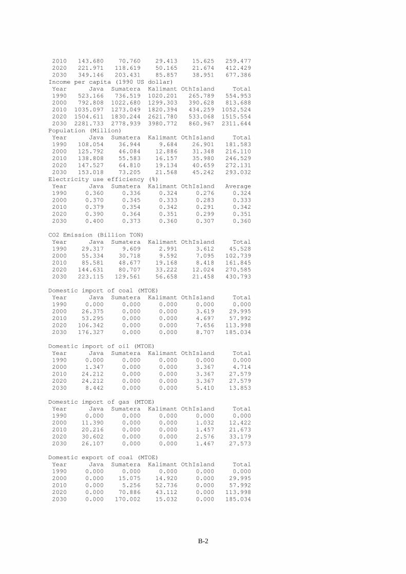
B-2

2010 143.680 70.760 29.413 15.625 259.477 2020 221.971 118.619 50.165 21.674 412.429 2030 349.146 203.431 85.857 38.951 677.386Income per capita (1990 US dollar) Year Java Sumatera Kalimant OthIsland Total 1990 523.166 736.519 1020.201 265.789 554.953 2000 792.808 1022.680 1299.303 390.628 813.688 2010 1035.097 1273.049 1820.394 434.259 1052.524 2020 1504.611 1830.244 2621.780 533.068 1515.554 2030 2281.733 2778.939 3980.772 860.967 2311.644Population (Million) Year Java Sumatera Kalimant OthIsland Total 1990 108.054 36.944 9.684 26.901 181.583 2000 125.792 46.084 12.886 31.348 216.110 2010 138.808 55.583 16.157 35.980 246.529 2020 147.527 64.810 19.134 40.659 272.131 2030 153.018 73.205 21.568 45.242 293.032Electricity use efficiency (%) Year Java Sumatera Kalimant OthIsland Average 1990 0.360 0.336 0.324 0.276 0.324 2000 0.370 0.345 0.333 0.283 0.333 2010 0.379 0.354 0.342 0.291 0.342 2020 0.390 0.364 0.351 0.299 0.351 2030 0.400 0.373 0.360 0.307 0.360

CO2 Emission (Billion TON) Year Java Sumatera Kalimant OthIsland Total 1990 29.317 9.609 2.991 3.612 45.528 2000 55.334 30.718 9.592 7.095 102.739 2010 85.581 48.677 19.168 8.418 161.845 2020 144.631 80.707 33.222 12.024 270.585 2030 223.115 129.561 56.658 21.458 430.793

Domestic import of coal (MTOE) Year Java Sumatera Kalimant OthIsland Total 1990 0.000 0.000 0.000 0.000 0.000 2000 26.375 0.000 0.000 3.619 29.995 2010 53.295 0.000 0.000 4.697 57.992 2020 106.342 0.000 0.000 7.656 113.998 2030 176.327 0.000 0.000 8.707 185.034

Domestic import of oil (MTOE) Year Java Sumatera Kalimant OthIsland Total 1990 0.000 0.000 0.000 0.000 0.000 2000 1.347 0.000 0.000 3.367 4.714 2010 24.212 0.000 0.000 3.367 27.579 2020 24.212 0.000 0.000 3.367 27.579 2030 8.442 0.000 0.000 5.410 13.853

Domestic import of gas (MTOE) Year Java Sumatera Kalimant OthIsland Total 1990 0.000 0.000 0.000 0.000 0.000 2000 11.390 0.000 0.000 1.032 12.422 2010 20.216 0.000 0.000 1.457 21.673 2020 30.602 0.000 0.000 2.576 33.179 2030 26.107 0.000 0.000 1.467 27.573

Domestic export of coal (MTOE) Year Java Sumatera Kalimant OthIsland Total 1990 0.000 0.000 0.000 0.000 0.000 2000 0.000 15.075 14.920 0.000 29.995 2010 0.000 5.256 52.736 0.000 57.992 2020 0.000 70.886 43.112 0.000 113.998 2030 0.000 170.002 15.032 0.000 185.034

B-3

Domestic export of oil (MTOE) Year Java Sumatera Kalimant OthIsland Total 1990 0.000 0.000 0.000 0.000 0.000 2000 0.000 4.714 0.000 0.000 4.714 2010 0.000 27.579 0.000 0.000 27.579 2020 0.000 27.579 0.000 0.000 27.579 2030 0.000 13.303 0.550 0.000 13.853

Domestic export of gas (MTOE) Year Java Sumatera Kalimant OthIsland Total 1990 0.000 0.000 0.000 0.000 0.000 2000 0.000 12.422 0.000 0.000 12.422 2010 0.000 21.168 0.505 0.000 21.673 2020 0.000 23.581 9.598 0.000 33.179 2030 0.000 8.839 18.735 0.000 27.573

Foreign import of coal (MTOE) Year Java Sumatera Kalimant OthIsland Total 1990 0.000 0.000 0.000 0.000 0.000 2000 0.000 0.000 0.000 0.000 0.000 2010 0.000 0.000 0.000 0.000 0.000 2020 0.000 0.000 0.000 0.000 0.000 2030 0.000 0.000 0.000 0.000 0.000

Foreign import of oil (MTOE) Year Java Sumatera Kalimant OthIsland Total 1990 0.000 0.000 0.000 0.000 0.000 2000 0.000 0.000 0.000 0.000 0.000 2010 11.692 0.000 0.000 1.542 13.234 2020 24.212 0.000 0.000 0.538 24.750 2030 8.442 0.000 0.000 0.187 8.630

Foreign import of gas (MTOE) Year Java Sumatera Kalimant OthIsland Total 1990 0.000 0.000 0.000 0.000 0.000 2000 0.000 0.000 0.000 0.000 0.000 2010 0.000 0.000 0.000 0.000 0.000 2020 0.000 0.000 0.000 0.000 0.000 2030 0.000 0.000 0.000 0.000 0.000

Demand sector (MTOE)REGION = 1 Year Industry Transport OtherSector 1990 16.949 10.084 18.609 2000 45.570 13.762 18.651 2010 71.710 20.777 21.295 2020 115.642 31.186 30.656 2030 173.032 45.914 43.227REGION = 2 Year Industry Transport OtherSector 1990 5.746 2.587 10.469 2000 29.046 4.293 10.477 2010 43.505 7.060 10.486 2020 72.575 11.694 11.321 2030 124.990 18.881 17.459REGION = 3 Year Industry Transport OtherSector 1990 2.330 1.075 2.144 2000 10.314 1.652 2.145 2010 18.033 2.963 2.838 2020 30.693 4.988 4.601 2030 52.752 8.037 7.120REGION = 4 Year Industry Transport OtherSector 1990 2.129 1.790 2.704

B-4

2000 6.886 1.790 2.713 2010 8.239 2.214 2.721 2020 11.838 3.334 3.809 2030 21.649 5.436 5.792

Electricity & nonelectricity energy (MTOE)REGION = 1 Year Industry Transport Other Total ELE NON ELE NON ELE NON ELE NON 1990 2.200 14.749 0.972 9.112 1.867 16.742 5.039 40.603 2000 9.320 36.250 0.994 12.768 1.909 16.742 12.223 65.759 2010 13.958 57.752 1.017 19.760 1.953 19.342 16.927 96.854 2020 21.874 93.769 1.040 30.146 1.997 28.658 24.911 152.573 2030 33.717 139.316 1.064 44.850 2.043 41.184 36.824 225.349REGION = 2 Year Industry Transport Other Total ELE NON ELE NON ELE NON ELE NON 1990 1.040 4.706 0.000 2.587 0.372 10.097 1.412 17.390 2000 2.822 26.224 0.000 4.293 0.380 10.097 3.202 40.614 2010 4.169 39.336 0.000 7.060 0.389 10.097 4.558 56.493 2020 6.845 65.730 0.000 11.694 0.398 10.923 7.243 88.347 2030 12.096 112.894 0.000 18.881 0.407 17.052 12.503 148.827REGION = 3 Year Industry Transport Other Total ELE NON ELE NON ELE NON ELE NON 1990 0.631 1.699 0.000 1.075 0.046 2.098 0.677 4.872 2000 1.002 9.312 0.000 1.652 0.047 2.098 1.049 13.063 2010 1.728 16.305 0.000 2.963 0.048 2.789 1.776 22.057 2020 2.895 27.798 0.000 4.988 0.050 4.552 2.944 37.338 2030 5.105 47.647 0.000 8.037 0.051 7.069 5.156 62.754REGION = 4 Year Industry Transport Other Total ELE NON ELE NON ELE NON ELE NON 1990 0.373 1.756 0.003 1.787 0.373 2.331 0.749 5.874 2000 1.647 5.239 0.003 1.787 0.382 2.331 2.031 9.357 2010 1.921 6.317 0.003 2.212 0.390 2.331 2.315 10.860 2020 2.563 9.276 0.003 3.331 0.399 3.409 2.965 16.016 2030 4.659 16.991 0.003 5.433 0.408 5.383 5.070 27.807

Electricity energy production by fuel (MTOE)REGION = 1 Year Coal Gas Oil Hydr. Geoth. Total 1990 0.612 0.173 2.708 0.678 0.868 5.039 2000 3.014 0.173 2.708 2.215 4.113 12.223 2010 7.718 0.173 2.708 2.215 4.113 16.927 2020 15.702 0.173 2.708 2.215 4.113 24.911 2030 27.615 0.173 2.708 2.215 4.113 36.824REGION = 2 Year Coal Gas Oil Hydr. Geoth. Total 1990 0.322 0.031 0.712 0.335 0.012 1.412 2000 0.322 0.031 2.502 0.335 0.012 3.202 2010 0.322 0.031 3.858 0.335 0.012 4.558 2020 0.322 0.031 6.543 0.335 0.012 7.243 2030 0.322 0.031 11.803 0.335 0.012 12.503REGION = 3 Year Coal Gas Oil Hydr. Geoth. Total 1990 0.107 0.023 0.409 0.137 0.001 0.677 2000 0.107 0.023 0.781 0.137 0.001 1.049 2010 0.107 0.023 1.508 0.137 0.001 1.776 2020 0.107 0.023 2.676 0.137 0.001 2.944 2030 0.107 0.023 4.888 0.137 0.001 5.156REGION = 4 Year Coal Gas Oil Hydr. Geoth. Total 1990 0.112 0.031 0.442 0.142 0.022 0.749 2000 0.112 0.031 0.442 0.142 1.304 2.031

B-5

2010 0.112 0.031 0.442 0.142 1.588 2.315 2020 0.112 0.031 0.442 0.588 1.792 2.965 2030 0.112 0.031 0.442 2.693 1.792 5.070

Production of all energy technology (MTOE)

REGION = 1 Year COAL-IND COAL-OTH GAS-IND GAS-TRA GAS-OTH 1990 2.442 0.132 3.852 0.404 2.604 2000 23.943 0.132 3.852 4.060 2.604 2010 45.445 0.132 3.852 11.052 2.604 2020 81.462 9.178 3.852 21.438 2.604 2030 127.009 21.704 3.852 36.142 2.604

Year OIL-IND OIL-TRA OIL-OTH BIO-OTH 1990 8.455 8.708 6.876 7.130 2000 8.455 8.708 6.876 7.130 2010 8.455 8.708 6.876 9.730 2020 8.455 8.708 6.876 10.000 2030 8.455 8.708 6.876 10.000

Year COAL-P GAS-P OIL-P HYDRO GEOTR 1990 0.612 0.173 2.708 0.678 0.868 2000 3.014 0.173 2.708 2.215 4.113 2010 7.718 0.173 2.708 2.215 4.113 2020 15.702 0.173 2.708 2.215 4.113 2030 27.615 0.173 2.708 2.215 4.113

REGION = 2 Year COAL-IND COAL-OTH GAS-IND GAS-TRA GAS-OTH 1990 0.422 0.011 0.942 0.017 1.102 2000 15.134 0.011 7.748 1.723 1.102 2010 33.293 0.011 2.702 4.490 1.102 2020 61.446 0.011 0.942 9.124 1.102 2030 92.488 0.011 17.064 16.311 1.102

Year OIL-IND OIL-TRA OIL-OTH BIO-OTH 1990 3.342 2.570 2.642 6.342 2000 3.342 2.570 2.642 6.342 2010 3.342 2.570 2.642 6.342 2020 3.342 2.570 2.642 7.168 2030 3.342 2.570 2.642 13.297

Year COAL-P GAS-P OIL-P HYDRO GEOTR 1990 0.322 0.031 0.712 0.335 0.012 2000 0.322 0.031 2.502 0.335 0.012 2010 0.322 0.031 3.858 0.335 0.012 2020 0.322 0.031 6.543 0.335 0.012 2030 0.322 0.031 11.803 0.335 0.012

REGION = 3 Year COAL-IND COAL-OTH GAS-IND GAS-TRA GAS-OTH 1990 0.015 0.002 0.542 0.002 0.002 2000 3.712 0.002 4.458 0.579 0.002 2010 13.609 0.002 1.554 1.890 0.002 2020 26.114 0.002 0.542 3.915 0.002 2030 45.963 0.002 0.542 6.964 0.002

Year OIL-IND OIL-TRA OIL-OTH BIO-OTH 1990 1.142 1.073 0.452 1.642 2000 1.142 1.073 0.452 1.642 2010 1.142 1.073 0.452 2.333 2020 1.142 1.073 0.452 4.096 2030 1.142 1.073 0.452 6.613

B-6

Year COAL-P GAS-P OIL-P HYDRO GEOTR 1990 0.107 0.023 0.409 0.137 0.001 2000 0.107 0.023 0.781 0.137 0.001 2010 0.107 0.023 1.508 0.137 0.001 2020 0.107 0.023 2.676 0.137 0.001 2030 0.107 0.023 4.888 0.137 0.001

REGION = 4 Year COAL-IND COAL-OTH GAS-IND GAS-TRA GAS-OTH 1990 0.022 0.002 0.582 0.005 0.003 2000 3.505 0.002 0.582 0.005 0.003 2010 4.583 0.002 0.582 0.430 0.003 2020 7.542 0.002 0.582 1.549 0.003 2030 15.257 0.002 0.582 1.608 0.003

Year OIL-IND OIL-TRA OIL-OTH BIO-OTH 1990 1.152 1.782 0.402 1.924 2000 1.152 1.782 0.402 1.924 2010 1.152 1.782 0.402 1.924 2020 1.152 1.782 0.402 3.002 2030 1.152 3.825 0.402 4.976

Year COAL-P GAS-P OIL-P HYDRO GEOTR 1990 0.112 0.031 0.442 0.142 0.022 2000 0.112 0.031 0.442 0.142 1.304 2010 0.112 0.031 0.442 0.142 1.588 2020 0.112 0.031 0.442 0.588 1.792 2030 0.112 0.031 0.442 2.693 1.792