An energy AGE model. Forecasting energy demand in Spain

An energy AGE model.

Forecasting energy demand in Spain.

ÓSCAR DEJUÁN, NURIA GÓMEZ, DIEGO PEDREGAL,

MARÍA ÁNGELES TOBARRA, JORGE ZAFRILLA

University of Castilla – La Mancha. Albacete (Spain). (July 2008)

[email protected]

Paper presented to the Input Output Meeting on Managing the Environment. Sevilla 9-11 July, 2008

An energy AGE model. 1

An energy AGE model. Forecasting energy demand in Spain.

ABSTRACT

The paper develops an Applied General Equilibrium (AGE) model for the estimation of energy demand and applies it to the Spanish Economy. The price system is based in the classical (Sraffian) theory of prices of production. The quantity system is based on the Keynesian principle of effective demand supported by broad energy multipliers. Both systems have been adapted to the specificities of energy industries. The model is dynamic in nature since output and technology are evolving through time. Energy technical coefficients are declining at a specific rate that may be speeded up or slowed down after changes in prices of the different sources of energy. The “tendencies” and “elasticities” implied are computed by calibration and econometric methods. Corresponding author: Oscar Dejuán Department of Economics and Finance. University of Castilla-La Mancha (UCLM). (Spain) e-mail: [email protected] Postal address: Facultad de Ciencias Económicas y Empresariales. Pz. Universidad, 1. 02071 Albacete (Spain)


1. Introduction 1

The purpose of this paper is to build an AGE (applied general equilibrium)

model combining elements of the Classical-Sraffian tradition and the Keynesian

one. The model will be applied for forecasting the demand for energy in the

Spanish economy in different scenarios and after different shocks. The time

span of our predictions will be one to five years. The questions to be answered

are of the following type: What will the path of energy demand be if the

economy enters into a recession (or into a boom)? What if the price of crude

doubles? What if natural gas producers receive a huge subsidy while petrol

refiners are heavily taxed? Although the purpose of this paper is restricted to

forecasting energy demand, there are obvious extensions into the analysis of

environment (emission of pollutants, exhaustion of natural resources and so

on).

The structure of the paper is as follows. Section 2 analyzes the structure

and technology implicit in an input-output table. Section 3 develops the quantity

system and derives the energy multipliers. Section 4 develops the price system

and adapts it to the specificities of energy industries. Section 5 integrates the

quantity and price systems and explores its dynamics. In section 6 we fill the

model with Spanish data and forecast energy demand in a couple of alternative

scenarios. Conclusions appear in section 7.

Before entering into the mechanics of our energy AGE model, we should

examine its alternatives2. Any overview of the literature should start with the

International Energy Agency (IEA) model (IEA: 2006 a; 2006 b; 2007). IEA

estimates worldwide demand for different types of energy in the very long run

(up to 25 years). We are looking for a more concrete model that takes into

1 Previous versions of this paper were presented by Oscar Dejuán at the Zaragoza Conference on Input-Output Economics (5-7 September 2007) and at the Eco-Mod Moscow Conference on “Energy and Environmental Modelling” (September 13-14, 2007). The proceedings of the last conference were edited by Ali Bayar (2008). The model was applied to forecast the demand for the six main products derived from petrol. The research was financed by Spanish CNE (Comisión Nacional de Energía). Other participants in the applied research, apart from the signatories of this paper, were M.A. Cadarso, C. Córcoles and E. Febrero. Our gratitude to them and to the CNE. 2 Our survey on the literature does not exhaust the variety of models in use. Kydes, Shaw & McDonald (1995) provides additional models and references.


account the specific technology of different sectors and households, in order to

make accurate predictions in a time span of one to five years. To gain

accuracy, we should tie mathematically the variables in a true AGE model,

showing the interrelationship between prices and quantities.

The use of econometric techniques to forecast energy demand has

increased in parallel to the availability of data. Econometric models focus on

elasticities, i.e. on the variation of energy demand after a small change in

income and prices (everything in percentage terms). They have problems

predicting the impact of big changes in prices, whose impact is usually

registered after several months (or years) and is not reversible3.

Input-output models are specialized in finding the direct and indirect links

between industries by means of a variety of multipliers4. They can compute the

demand for energy (or the pollution resulting from it) after the expansion of any

industry. By means of social accounting matrices (SAM) they can even trace

the path of income from the moment it is received by factors to the moment it is

spent by households. These models, however, cannot analyze the impact on

energy demand associated to changes in energy prices. Neither can they

endogeneize technical progress.

Neoclassical CGE (Computable General Equilibrium), models are well

equipped for the integration of the price and the quantity system5. EcoMod has

developed specific software (GAMS) for that purpose. The possibility of

substitution among factors of production and among consumption goods is a

remarkable feature of the model. The strong and immediate influence of

demand on prices, and of prices on the quantities demanded is another one.

3 Studies focusing on energy consumption by households: Galli, 1998; Gately & Huntington, 2002; Labandeira et al, 2006, Lenzen, 2006. Dynamic studies: Judson et al, 1999; Olatubi & Zhang, 2003, Roca & Alcántara, 2002. 4 Some useful references may be: Alcantara & Padilla, 2003; Casler & Willbur, 1984; Dejuán, Cadarso & Córcoles, 1994; Duchin, 1998; Galli, 1998; Manresa, Sancho & Vegara, 1998; McKibbin & Wilcoxen, 1993; Miyazawa & Masegi, 1963; Pyatt and Round, 1985; Roca & Serrano, 2007; Sun, 1998; Vringer & Blok, 1995. 5 An overview of the neoclassical CGE models can start with Kehoe & Kehoe (1994); Kehoe, Srinivasan & Whalley, eds (2004), Gibson & Seventer, 2000; Ginsburgh & Keyzer (2002). Neoclassical CGE models related to energy are: André, Cardenete & Velázquez (2005), Capros et al (1996), Ferguson et al (2005), Hanley et al (2006), Roson (2003), Welsch & Ehrenheim (2004).


Despite the great and ingenious versatility of GAMS we have decided to

build a personal model closer to the Classical – Keynesian theory and to the

real economy we intend exploring (Dejuán 2006 and 2007 justifies the option).

The main features of our energy model are the following ones:

(1) It is an “energy model” nested in a general equilibrium context. Parameters

of non-energy sectors are derived directly from the IOT. We take them as

given data until a new table is released. By contrast, energy parameters

are obtained checking a variety of sources and they are allowed to change

endogenously. This “dual” treatment of energy and non-energy sectors is a

crucial simplification to make our model manageable.

(2) It is a “hybrid model” that combines input-output techniques with

econometric methods. From input-output tables (IOT) we obtain, via

“calibration”, technical coefficients, consumption patterns and import

propensities. Econometrics informs how significant and robust these

parameters are. It also helps finding out price elasticities and technological

trends that cannot be derived from input-output tables.

(3) It is a dynamic and sequential model in the sense that some key variables

convey an implicit rate of growth or decline. Autonomous demand grows at

an exogenous rate. Technical progress brings about a continuous

reduction of energy coefficients. This trend may be accelerated or delayed if

there are significant movements in the relative prices of the different

sources of energy. Changes occur sequentially and, by and large, they are

irreversible.

(4) The quantity system is based on the Keynesian principle of effective

demand and the multiplier mechanism (Keynes, 1936). It states that the

level production at year t (and energy demand) is a multiple of the expected

level of autonomous demand for the same period. By the same token, the

growth of output and of energy demand will be related to the growth of

autonomous demand.

(5) The price system is based on the Classical theory of prices of production. It

has been updated by Sraffa (1960) and goes back to Ricardo (1817). It


contends that goods exit factories with a price label. The cost of production

(which includes the “normal” rate of profit) determines this price and plays

the role of a gravity centre for market prices. The special features of energy

prices do not prevent their integration into a price of production model.

2. An input-output table and model useful for the analysis of energy.

The economy we are considering can be represented by a symmetric IOT, at

basic prices. The last symmetric IOT released in Spain corresponds to the year

2000 and considers 73 industries. Each one is identified with the homogeneous

commodity it produces. There is a make and use matrix for 2004 but we cannot

rely in it since the production process is very important for our purposes.

Our “energy input-output” has 18 industries. Each of the 18 industries we

consider shall be identified with the homogenous commodity it produces. The

first four columns and rows correspond to the four energy sources we are

considering:

1. Petrol (refining and distribution);

2. Gas (gasification and distribution);

3. Electricity (generation and distribution);

4. Coal (extraction and distribution).

The remaining industries of the Spanish input-output table appear highly

aggregated. Nevertheless we keep separated the industries which consume

more energy. They are the four producers of energy and the four transport

services (by train, land, sea and air). Agriculture, Chemistry-Plastics and

Restoration-Hotels do also stand out as big energy consumers.

Households consume plenty of energy. This fact justifies the

endogeneization of households’ consumption. It will become our “n” industry

(“19” to be more precise). The 19 column gathers final induced consumption by

households. We exclude final consumption by tourists that is clearly

“autonomous”, i.e. not dependent on current income generated in the country.


The 19 row gathers the part of value added that finance induced final

consumption. Since the household sector does not generate value added, the

19 row adds up to the value of the 19 column. We know that there is a high

and stable relationship between households’ disposable income and final

induced consumption. We have also realized that there a stable relationship

between value added and final induced consumption. In Spain, during the last

two decades, 64% of gross value added has been devoted to final consumption.

(The R2 of the regression is 0,9). This finding authorizes us to compute the 19

row by extracting in each industry the percentage necessary to finance final

consumption by households.

Table 1: Spanish input-output table (2000)

Table 1.1 shows the structure of our energy input-output table. As its is

well known, an IOT can be read horizontally (as in [2.1]) or vertically (as in [2.2]

and [2.3]). The vertical reading explains the cost structure of each industry:

cost of intermediate inputs and cost of primary inputs (factors of production who

receive value added). A horizontal reading shows the allocation of each

commodity among intermediate and final uses.

qYZMYMZ ddy =+=−+− ')'()( [2.1]

qPIMZPIZ d =++=+ ')(' [2.2]

qPIZ =+' [2.3]

q is the vector of total output produced in the economy (domestic production).

In [2.1] it appears as a column vector. In [2.2] and [2.3] it appears as a row

vector.

Z is a square matrix with n columns (industries) and n rows (goods). It accounts

for intermediate consumption by industries and induced final consumption by

households. It describes sales of good i when we read horizontally; purchases

by industry j when we read vertically.

Zd results from subtracting imports of intermediate goods (M) from Z.

Z’ is the proper interindustry table. It is derived from Z, after equating to zero

the cells of the last row corresponding to the finance of induced consumption.


Y stands for final demand. It is a rectangular matrix with n rows and four

columns: final consumption by households, government’s final consumption,

gross investment and exports)

Y’ stands for final autonomous demand. It is a matrix similar to Y but in the first

column we only include autonomous consumption by households. We can

withdraw the column altogether and include final consumption by tourists in the

export column.

Y’d results from subtracting imports of final goods from Y’.

M is a n·n square matrix gathering the imports of each commodity by each

industry.

My is a rectangular matrix of n rows (one for each commodity) and 3 columns

(one for each element of final autonomous demand).

PI is a rectangular matrix of “primary inputs” or “non produced inputs”. It has n

columns and 6 rows. Row W stands for wages; B for profits; T1 for specific

indirect taxes (net of subsidies) on energy sources; T2 for value added tax,

other indirect taxes and other rents; COG for imports of crude oil and gas by

industries 1 and 2.

PI’ results from subtracting from PI the percentage of value added devoted to

finance induced consumption.

Dividing these matrices and vectors by the corresponding value of

sectoral output (q) we obtain the matrices and vectors expressing the average

technology of each industry 6.

(a) Matrix of (total) technical coefficients:

( ) 1ˆ· −= qZAt [2.4]

6 Some comments on notations are necessary at this point. (a) Diagonal matrices are identified by angular brackets (<q>) or by a circumflex ( q̂ ). “I” is the identity matrix. (b) Unless otherwise stated the order of the matrix is n·n, being n the number of industries. Households occupy the last position, i.e. the 19tth. (c) In other cases, the order of the matrix or vector appears inside a parenthesis with two figures separated by a dot; the first one refers to the number of rows; the second, to the number of columns. (d) The single figure in a parenthesis refers to the year under consideration, being (0) the base year. (e) A dot indicates matrix multiplication. ⊗ indicates cell by cell multiplication.


(b) Matrix of import coefficients (imports per unit of output):

( ) 1ˆ· −= qMAm [2.5]

We can obtain Am multiplying At by m. m is a (n·n) matrix of “import shares” or

“import propensities” derived from the original tables.

mAA tm ⊗= [2.6]

(c) Matrix of domestic coefficients:

( ) )(ˆ· 1 miiAAAqZA tmtdd −⊗=−== − [2.7]

“ii” is a unit matrix with ones in all cells. We subtract import shares and multiply

the result by At. The result is the matrix of domestic technical coefficients (Ad)

with is the main ingredient of the multipliers.

(d) Vector of primary inputs shares:

( ) 1ˆ· −= qPIv [2.8]

v is a row vector which expresses the share of primary inputs in the value of

total production (q). Alternatively we can present it as a rectangular matrix with

as many columns as industries and six rows corresponding to the share of

wages (α), the share of profits (β), the share of indirect taxes on energy (γ), the

share of other indirect taxes and rents (δ), and the share of imported crude oil

and gas. Note that the last (n) cell of α and β are zero, because households do

not generate value added. Conversely, all the cells of γ and δ are nil except the

last one, because in a system of base prices, indirect taxes are paid by

households. Vector λ only shows positive figures in cells 1 and 2, corresponding

to petrol refining and regasification and distribution of gas 7.

In a disaggregated fashion we can rewrite [2.7] as:

7 In the Spanish IOT this is not always the case, since γ and δ include the part of indirect taxes that cannot be transferred to final consumers.


⎥⎥⎥⎥⎥⎥

⎦

⎤

⎢⎢⎢⎢⎢⎢

⎣

⎡

========

==

=

00...0...000...00

0...0...

21

21

21

21

21

nm

nm

nm

nm

nm

v

λλλλδδδδγγγγ

ββββαααα

[2.9]

Matrices and vectors in [2.3] till [2.6] contain the basic coefficients of the

input-output model from which we shall derive the main tools of analysis

namely: multipliers and price equations. Technical coefficients and propensities

are supposed to remain constant during the period of analysis (from the date of

publication of IOT to the date of our previsions). This is the general rule. It

does not apply to the rows of energy producing sectors. The competitive

pressure to save energy is stronger than for any other intermediate good

because energy prices are more volatile and represent a huge part of costs. In

section 5 we shall explain how energy coefficients are adapted from the year

IOT are released to the year our forecasts are projected.

3. The quantity system and the energy multipliers.

The inverse of Leontief corresponding to the expanded domestic coefficients

matrix (Ad) can be identified with the multiplier of total output. All the other

multipliers derive from it.

[ ] 1)19·19(

−−= dAIMQ [3.1]

The first column of [3.1] shows the impact of the expansion of industry 1

(refined petrol in our case) on the production of the remaining industries. By

reading the cells of the column we can even identify the specific contribution of

each industry to the global impact on output. It is a broad multiplier because it

gathers: (a) intermediate goods directly used in the production of autonomous

demand; (b) intermediate goods indirectly required in the production of

autonomous demand; (c) consumption goods purchased by the workers

employed, directly or indirectly, in the production of autonomous demand.


Total output of the economy at the base year (0) can be computed as a

multiple of the vector of domestic autonomous demand for the same period.

[ ] )1·19)(0()1·19)(0(1· qYAI dd =− − [3.2] 8

The multiplier of income is computed by [3.3]. v is the row vector

represented by [2.5]. It expresses the share of primary inputs in the value of

total output.

[ ] 1)19·1()19·1( · −−= dAIvMv [3.3]

The multiplier of employment and the multiplier of energy could be

computed in a similar fashion (Dejuán & Febrero, 2000). First we fill the vectors

of direct requirements of labour (l) and different sources of energy (E). Then we

post-multiply these vectors by MQ. The singularity regarding energy multipliers

is that energy requirements are already accounted for in the matrix of technical

coefficients. Rows 1 to 4 of At and Ad gather the unit requirements of refined

petrol, gas, electricity and coal. Consequently, the energy multiplier will be a

rectangular matrix coinciding with the first four rows of matrix MQ. To detach

the energy rows from the Leontief’s inverse we premultipy MQ by a unit matrix

(i). It has 19 rows and columns and rows. The first 4 rows are “ones”, the

remaining ones are “zeros”.

[ ] 1)19·4()19·4(

−−⊗= dAIiME [3.4]

The interpretation of the energy multiplier is the usual one. Column j

computes the demand for the four energy products dragged (directly or

indirectly) by the production of one additional unit in industry j.

8 There are different ways to derive the structural multiplier. All of them may be correct and compatible provided they are interpreted properly. The theoretical perspective does also matters for the computation and interpretation of the multipliers. Miyazawa & Masegi (1963) and Kurz (1985) adopt a Classical-Keynesian perspective akin to our theoretical model. In a previous paper (Dejuán, Cadarso, Córcoles, 1994) we added induced final consumption directly to the cells of the original m·m table. Here we have followed the more common procedure of adding a column and a row corresponding to the household sector (m+1=n). When using the last procedure we should have in mind that the n cell of q should not be added to the preceding ones. The reason being that national accounts do not consider “human capital” as part of total output.


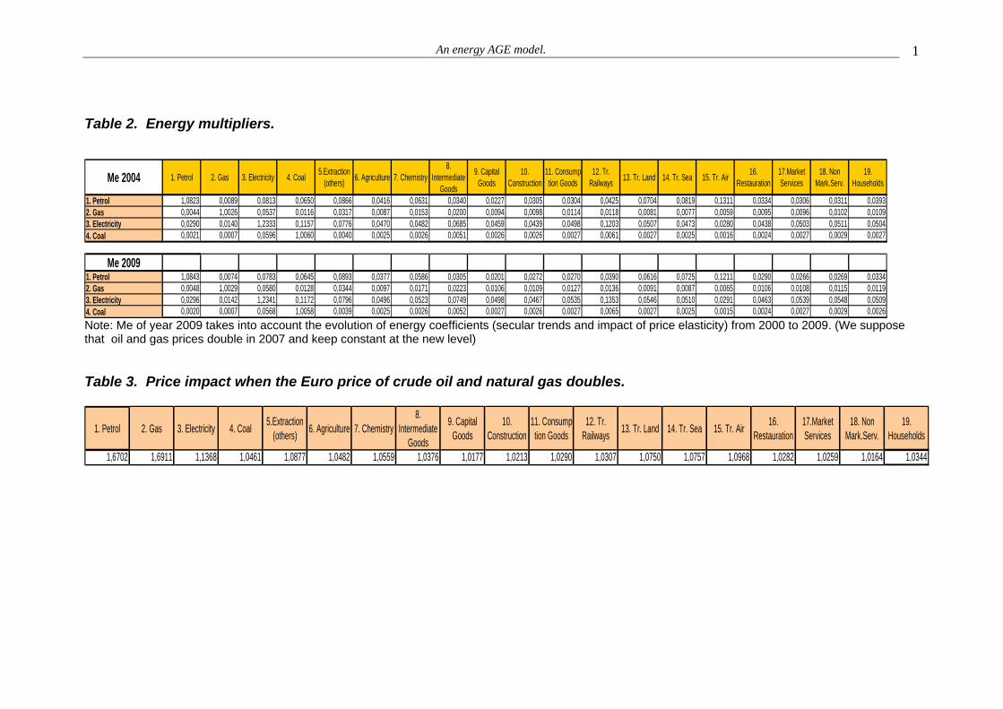
Table 2: Energy multipliers

The energy demand has a variety of applications. We can predict the

increase in different energy sources associated to an increase of final

autonomous demand. The increase may be harmonic or differentiated by

expenditures (private investment, public expenditures, exports…) or by goods

(petrol, cars, …).

Our quantity model and the multiplier that results from it are based on

Keynes principle of effective demand. According to this principle the level of

output at year t does not depend on capacity installed and/or on the available

labour supply. In addition it is independent on prices. The level of output is

supposed to be a multiple of expected autonomous demand for the year under

consideration. The principle can be extrapolated in time to conclude that the

paths of output, employment and energy demand will depend on the expected

growth of autonomous demand. The vector of autonomous demand at the base

year (Y’(0)) and its expected rate of growth (gy) are the key exogenous variables

of a Keynesian AGE model.

The working of the multiplier mechanism requires firms to have some

spare capacity and stocks. Otherwise they could not increase production to

match unexpected increases in demand. As a matter of fact, modern technology

has evolved in order to make easier adjustments through capacity utilization. In

most industries, the desired degree of capacity utilization is far below the

engineering or technical limit. This margin allows firms to match the peaks of

demand by using the installed capacity more hours per day during boom

periods

The demand for electricity and gas follow the Keynesian pattern: supply

follows demand. This is not the case for the coal industry and, most of all, for

petrol one. Refineries are usually operated 24 hours a day, so the possibility to

adjust to demand increases via capacity is negligible. Petrol stocks are

significant but they cannot cope either with a big and prolonged increase in

demand. Refineries are supposed have to forecast accurately the permanent


increases in demand and increase capacity in advance. If the increases in

demand are too big and / or unexpected, the adjustment will occur via imports.

The matrix of import shares (m) cannot be considered fixed, Coefficients

in the first and fourth rows (corresponding to refined petrol and coal) will depend

on the expected rate of growth (apart from the gap between national and

international prices).

The main conclusion to be emphasized at this point is that changes in

demand do not alter prices. In the next sections we are going to see that prices

are supply determined, i.e. they depend on technology and distribution. We

shall also see that prices changes exert only a tiny influence on the quantities

demanded via the alteration of technical coefficients.

4. The price system.

A vertical reading of the IOT (as it was done in [2.3]), shows the cost structure

of the n industries of the economy. After dividing each column j by the value of

the sectoral output (qj) we obtain the unit costs. By construction each column of

coefficients adds up to one

[ ]1...11)( =++++++=++ λγδβαmdmd AAvAA [4.1]

We can interpret the elements of [4.1] as the product of undetermined

quantities of outputs, inputs and factors by their respective prices, prices that

have been set equal to one. We are not saying that one ton of petrol is worth

one million euros (1 M€). We simply say that an undefined quantity of petrol is

worth 1 M€. We also state that in order to produce it, we need (for instance) 0,2

undefined units of electricity (whose unit price is 1 M€) and 0,05 undefined units

of labour (each unit gaining 1 M€).

This assumption allows us to write the price of the good produced by

industry j as the value of domestic inputs per unit of output, the unit value of

imported inputs (crude oil and natural gas are included in λ), the unit labour

costs (α), the unit profit (β), and the unit indirect taxes (γ, δ). γ refers to special


taxes on energy, that in a system of base prices are charged on households

(cell 19). δ gathers net value added tax (also translated to final consumers) and

net extra profits and rents per unit of output. We remind that A’ is the matrix of

technical coefficients, after equating to zero the last row, corresponding to the

household sector. In matrix notation we can write:

( ) ( ) [ ]1...11)('·'· )19·1()19,1()19·1()19·1()19·1( =++++++= λδγβαiApApp mm [4.2]

The price of refined petrol (to choose an example) could be computed in the

following way:

)(·· 1111119

1'

1,19

1'

1,1 λδγβα ++++++= ∑∑ == i imii idi ApApp [4.3]

The preceding expression is not a theory of prices, but a description of

how prices are made up. To have a proper theory of prices we should introduce

all the equilibrium conditions. In competitive markets prices may fulfil two

conditions: (a) They cover full costs of production which includes “normal

profits”. (b) They warrant a “normal”, “general” or “uniform” rate of profit (r*) on

the fixed capital invested. Relative prices are supposed to move until the last

100 M€ invested in any industry yield the same profit. The first part of [4.3]

(below) computes unit profits in industry 1 as r* times the value of fixed capital

installed (pi·kij). Since IOTs do not inform about fixed capital requirements we

can express profits as a net margin (b’) on circulating capital (the value of

intermediate goods domestically produced or imported). Notice that the rate of

profit is uniform across the industries (r1=r2=r*), while sectoral profit margins are

different (b’1≠b’2). If industry 1 is capital intensive, b’1>b’2 is a condition to

obtain the general and uniform rate of profit in both industries.

( ) ( )∑ ∑∑ +==19

1

19

1 1,,1119

1 11 ···'·'· imimiiii apapbkprβ [4.4]

Notice also that the tendency to a uniform rate of profit is a long run

phenomenon. In the short run some firms will get extraprofits while other will


suffers economic losses (i.e. profits below average). They are encapsulated in

the row vector δ, that do also account for other indirect taxes and subsidies) 9.

Let us define gross profit margins as bj=(1+b’j) and introduce them into

[4.2]. We obtain the competitive system of prices that can be expressed either

in an additive or a multiplicative way. In

[ ]1...11)(ˆ··ˆ·· =+++++= λδγαbApbApp mm [4.5]

[ ] [ ]1...11ˆ·)··(1=−++++=

−bAIApp mmλδγα [4.6]

The preceding equations allow us to compute changes in relative prices

after a variety of “shocks” impinging on technology, distribution and

redistribution (taxes and subsidies). A rise in nominal wages, for example, will

push all prices up (as in an inflationary process). But the highest price

increases will occur in labour intensive and petrol intensive commodities.

The Classical or Sraffian theory of prices of production apply to

“reproducible” commodities under competitive conditions. The bulk of goods of

an IOT adjust in fact to the cost of production patterns. Energy products may

be an exception for a variety of reasons. Notwithstanding, we are going to show

that our model is well suited to tackle the special features of energy prices.

(a) Strong dependence on natural resources (crude oil and natural gas). In a

situation of scarcity, demand recovers full prominence in the determination

of prices. This conclusion applies only to big changes in the international

demand for crude petrol and natural gas that we take as given. Changes in

domestic demand, no matter how big they are, do not influence international

prices. To compute the effects on prices of an increase of the international

9 To obtain equilibrium prices it is necessary to link profits with any measure of the capital invested. There are different ways to do so (Sekerka et al., 1998; Brody, 1970). Surprisingly, the competitive long-term equilibrium condition is absent in neoclassical CGE models. Even if they start in a competitive equilibrium, prices cease to be in equilibrium after a shock. The new computed prices do not warrant a uniform rate of profit in any meaningful sense. In our opinion this is the main shortcoming of the CGE price system.


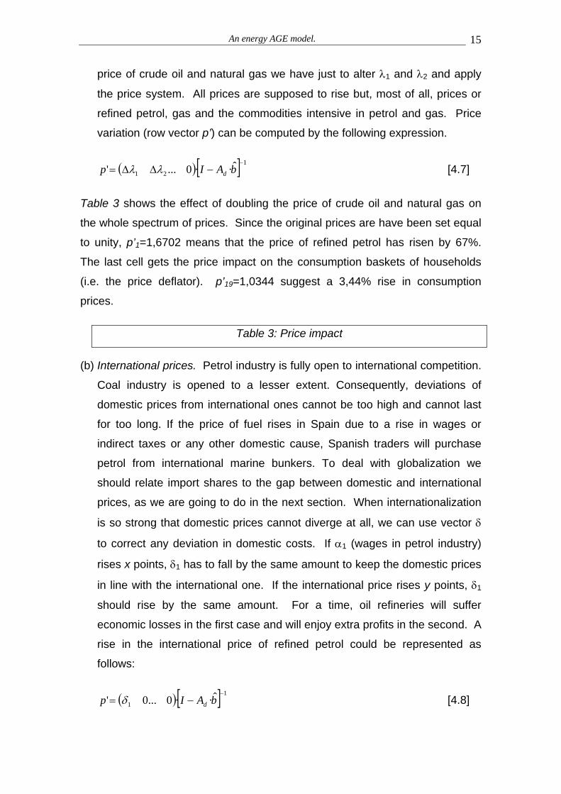
price of crude oil and natural gas we have just to alter λ1 and λ2 and apply

the price system. All prices are supposed to rise but, most of all, prices or

refined petrol, gas and the commodities intensive in petrol and gas. Price

variation (row vector p’) can be computed by the following expression.

( )[ ] 1

21ˆ··0...'−

−ΔΔ= bAIp dλλ [4.7]

Table 3 shows the effect of doubling the price of crude oil and natural gas on

the whole spectrum of prices. Since the original prices are have been set equal

to unity, p’1=1,6702 means that the price of refined petrol has risen by 67%.

The last cell gets the price impact on the consumption baskets of households

(i.e. the price deflator). p’19=1,0344 suggest a 3,44% rise in consumption

prices.

Table 3: Price impact

(b) International prices. Petrol industry is fully open to international competition.

Coal industry is opened to a lesser extent. Consequently, deviations of

domestic prices from international ones cannot be too high and cannot last

for too long. If the price of fuel rises in Spain due to a rise in wages or

indirect taxes or any other domestic cause, Spanish traders will purchase

petrol from international marine bunkers. To deal with globalization we

should relate import shares to the gap between domestic and international

prices, as we are going to do in the next section. When internationalization

is so strong that domestic prices cannot diverge at all, we can use vector δ

to correct any deviation in domestic costs. If α1 (wages in petrol industry)

rises x points, δ1 has to fall by the same amount to keep the domestic prices

in line with the international one. If the international price rises y points, δ1

should rise by the same amount. For a time, oil refineries will suffer

economic losses in the first case and will enjoy extra profits in the second. A

rise in the international price of refined petrol could be represented as

follows:

( )[ ] 1

1ˆ··0...0'−

−= bAIp dδ [4.8]


(c) Oligopoly and price regulation in gas and electricity. There are few

producers in each industry. Their chances to collude in order to fix prices

are enhanced. To avoid this outcome, government creates national

agencies that regulate prices of public utilities (electricity and gas, in

particular). As a matter of fact, regulators allow to increase prices in

proportion to changes in costs. They perform the same task as our

mathematical model (equation [4.6]), although with some delay.

(d) Specific taxes and subsidies. Some energy products support heavy indirect

specific taxes (refined petrol is the outstanding example). Other products

(like domestic coal) enjoy huge subsidies. Row γ accounts for specific taxes

on energy (net of subsidies). If taxes on petrol consumption (by firms and

households) double, the price of petrol will increase a lot and will reverberate

on the prices of all whole spectrum of commodities. Since we deal with IOT

at base prices, any change in taxes and subsidies will show up in δ19, the

cell corresponding to households. It will only affect consumer prices. We

could also simulate that the tax on fuels and the subsidy on domestic coal is

charged to the is charged to the corresponding sectors. Then we could see

how it impinges on market prices10.

( )[ ] 1

41ˆ··0...000'−

−∇Δ= bAIp dδδ

5. Dynamics of the system: tendencies and elasticities.

Our AGE model is dynamic one because some exogenous variables and some

parameters are continuously moving. The vector of final autonomous demand

is the “motor” of the system. The economy will grow in accordance to the rates

of growth of the elements of autonomous demand, rates that we take

exogenously. Technological parameters, consumption propensities and import

shares are taken as data but they cannot be considered “constant”. In this

section we are going to see the patterns of evolution of these parameters,

10 The only purpose of the simulation is to see the impact on market prices of a change in taxation. We shouldn’t mix magnitudes at base prices with magnitudes at market prices.


propensities and shares. We shall distinguish between secular trends

associated to technical change and short term deviations from the trend

explained by price elasticities.

(a) Secular trends of technical coefficients.

Technical coefficients of matrix At were obtained directly from the original IOT.

Every five years, or so, a fresh symmetrical IOT is released with new

coefficients reflecting technical change and, perhaps, a different mix in the

goods that fill the basket of commodities produced in each industry. Keeping

constant technical coefficients during five years seems plausible for most

inputs. Not so for energy products which depend on a natural resource whose

reproduction is not possible or takes long time. Under these circumstances,

energy prices will be more volatile with a tendency to grow. Firms will try to

save these resources and search for substitutes. This evidence justifies their

yearly updating of energy coefficients, most of all in a study focusing on

demand for energy11.

It is the moment to open the black box of technology and analyze the

typical energy coefficient (aij) of matrix At. We shall examine the coefficient in

the base year (0) and its evolution through time (five years). Let’s call τ the

“technological trend” or “inner tendency of technical coefficients”. A negative

τ(1.19) implies an improvement in technology: there is less petrol in the basket

purchased by households because new cars have reduced fuel consumption. A

positive trend like τ(2,19) indicates that more gas enters into the consumption

basket because petrol-heating is being substituted by gas-heating.

These trends may be influenced by previous changes in relative prices,

but they are independent of current movements in prices. To simplify, we’ll

suppose at this moment that prices remain constant. The evolution of the

matrix of technical coefficients (At(0) in the base year) can be traced by the

following equations. (1+τ) is a matrix of order 19·19 although all the rows are

11 We also observe a strong tendency towards a “labour saving technical change”. But the increases in labour productivity have been absorbed by wages. The unit labour cost has been kept rather constant for many years. Such “matching effect” has not been registered with respect to energy costs per unit of output.


zero except the four producing and distributing energy. In the cells

corresponding to these rows we find the secular trend plus one.

4)0()4(

3)0()3(

2)0()2(

1)0()1(

)1·(

)1·(

)1·(

)1·(

ijtt

ijtt

ijtt

tt

AA

AA

AA

AA

τ

τ

τ

τ

+=

+=

+=

+=

[5.1]

Table 4: Secular tendencies of energy coefficients.

Table 3 shows the tendencies we have found. There is a τ for each

energy source (petrol, gas, electricity and coal) and for each of the five sectors

considered (energy, other industries, transports, others services and

households). To find the precise numbers we have combined calibration and

econometric methods. The analysis of previous input-output tables has been

useful to differentiate the evolution of energy coefficients by industries.

Our analysis has relied mostly on “calibration”. We know the true

demand for petrol, gas, electricity and coal in years 2001 to 2006. If out model

is correct, we should obtain these figures multiplying the vector of final

autonomous demand times the energy multipliers. We adjust the matrix of

tendencies so that we obtain for years 2001 to 2006 the technical coefficients

and the energy multipliers that bring about the true (known) results.

Econometrics provides some useful hints. It gives some values for

tendencies and price elasticities informing about the reliability (R2) of the

parameters estimated. Particularly helpful has been the method of “non

observable components” (Harvey, 1989; Young, Pedregal & Tych, 1999). It

yields price elasticities and the inner tendencies of parameters that are

unrelated to current price movements. The estimates obtained from this

technique cannot be directly incorporated to our model because the energy

sources and the industries considered are not the same. Yet these estimates

provide a useful check for the values obtained by calibration.

(b) The impact of price-elasticity on technical coefficients.


Econometric studies (quoted in footnote 3 in section 1) show that price elasticity

is very low, at least in the short run. Energy demand is hardly altered by

movements in the relative prices of energy. In our model prices affect demand

indirectly, through technical change. A (strong) increase in the price of petrol

will accelerate the tendency to save fuels in industries and households. The

negative τ will increase in absolute value. A rise in the price of gas will

decelerate the tendency to use more gas per unit of output in the different

industries and households. The positive τ will decrease.

Economists distinguish between cross elasticity and own price elasticity.

The first one measures the percentage variation in the quantity consumed of

commodity i when the relative price of commodity j changes in a given

proportion. If the price of fuel rises over and above the price of gas, the

tendency to shift from fuel-heating to gas-heating will be accentuated. The

impact will take several months (even years) to be implemented. It will be

incorporated to the tendencies that are revised from time to time. We should

write a lower τ(1,19) and a higher τ(2,19) ).

Own price elasticity measures the percentage variation (always negative)

in the demand of commodity i when its price rises in a given percentage. If the

price of petrol and electricity doubles people will save some unnecessary drives

and, more frequently, will switch off electrical appliances when they are not in

use. Firms do have more difficulties to save energy at once because its

consumption is a technical requirement. Table 4 shows the estimated price

elasticity for households, only for the cases they are statistically significant.

Table 5: Price elasticities.

Figures in this table reflect the impact on quantities demanded when the

price doubles (one hundred percent increase). If the increase in price has been

25% we have to multiply the number given in table 5 times 0,25. In matrix

notation we obtain the impact on the energy demanded by multiplying the

diagonal matrix of price deviations (<pd>) times the matrix of price elasticities (ε


in table 4)12. We add this result to the matrix or secular tendencies to obtain the

matrix of “adjusted tendencies” (τ*).

)19·19()19·19()19·19(*

)19·19( ·εττ pd+= [5.2]

The evolution of the matrix of technical coefficients (At) from year 0 to

year 4 will be described by the following equations. Notice that we have

substituted matrix τ of [5.1] by matrix τ*.

)1(...

)1(

**)4(

*)5(

**)0(

*)1(

τ

τ

+⊗=

+⊗=

tt

tt

AA

AA [5.3]

(c)) Variations of import shares and import coefficients.

The energy multipliers are based on the matrix of domestic coefficients (Ad).

We know from [2.7] and [2.6] that Ad=At-Am and that Am=At⊗m. Am is the matrix

of import coefficients. m is the matrix of import shares. There is not warranty

that these shares remain constant through time. They may change if there is a

gap between domestic and international prices. They also increase, when firms

are unable to increase domestic production at the same rhythm than demand.

Let’s define εm as the price elasticity of imports. It is a n·n matrix

although all shares in the same row tend to be equal (import propensity of good

i is independent on the industry that purchases it). We focus only in the four

energy rows. And we fill only the elasticities that have proved to be

econometrically significant.

Table 6: Import elasticities.

12 We remind that the initial prices have been set equal to one (p). After a change in costs the price equations render vector p’. Price deviation of commodity i will be:

1'

−=−

= ii

iii p

ppp

pd


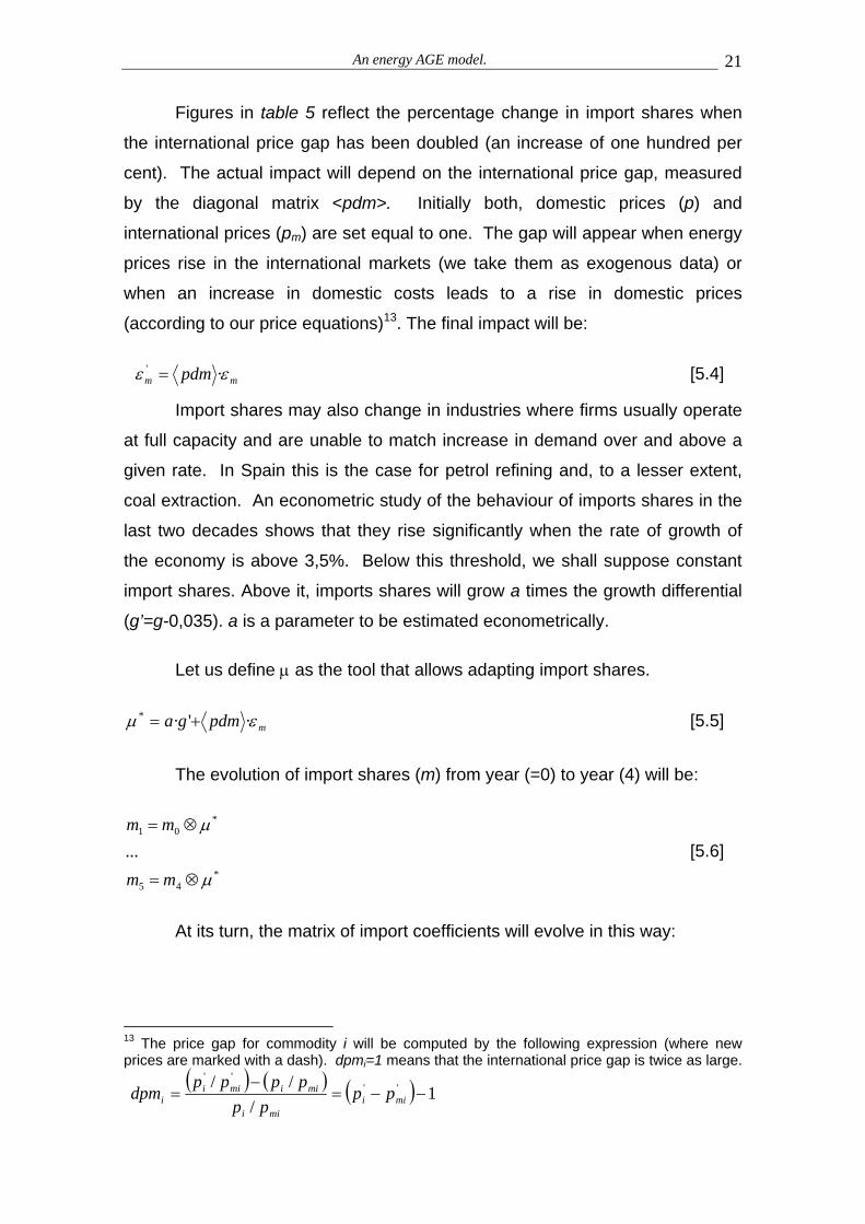
Figures in table 5 reflect the percentage change in import shares when

the international price gap has been doubled (an increase of one hundred per

cent). The actual impact will depend on the international price gap, measured

by the diagonal matrix <pdm>. Initially both, domestic prices (p) and

international prices (pm) are set equal to one. The gap will appear when energy

prices rise in the international markets (we take them as exogenous data) or

when an increase in domestic costs leads to a rise in domestic prices

(according to our price equations)13. The final impact will be:

mm pdm εε · ' = [5.4]

Import shares may also change in industries where firms usually operate

at full capacity and are unable to match increase in demand over and above a

given rate. In Spain this is the case for petrol refining and, to a lesser extent,

coal extraction. An econometric study of the behaviour of imports shares in the

last two decades shows that they rise significantly when the rate of growth of

the economy is above 3,5%. Below this threshold, we shall suppose constant

import shares. Above it, imports shares will grow a times the growth differential

(g’=g-0,035). a is a parameter to be estimated econometrically.

Let us define μ as the tool that allows adapting import shares.

mpdmga εμ ·'·* += [5.5]

The evolution of import shares (m) from year (=0) to year (4) will be:

*45

*01

...μ

μ

⊗=

⊗=

mm

mm [5.6]

At its turn, the matrix of import coefficients will evolve in this way:

13 The price gap for commodity i will be computed by the following expression (where new prices are marked with a dash). dpmi=1 means that the international price gap is twice as large.

( ) ( ) ( ) 1/

// ''

''

−−=−

= miimii

miimiii pp

ppppppdpm


*45

*01

...μ

μ

⊗=

⊗=

mm

mm [5.7]

A couple of observations are in order before closing the section on

technology.

(1) The impact of prices on elasticities are distributed in several years. But

they are not perpetual. The release of a new IOT marks a new starting point.

(2) Energy-saving technical change is not reversible. This is the so called

“ratchet effect”, that will be illustrated with two examples. (a) Households that

shift from petrol heating to gas heating after a rise in petrol prices, will not go

back to the original heating system when prices recover their previous levels.

(b) In an age of rising and volatile oil prices, the car industry is interested in

producing motors with low petrol consumption. The industry will not go back to

previous models even if oil prices stabilized at very low levels.

6. Forecasting energy demand in Spain.

Our AGE model has been designed to forecast energy demand under different

scenarios during a period of five years. The key parameters of the scenario are

the expected rate of growth of the economy (that depends on the expected rate

of growth of autonomous final demand, Y’) and the Euro price of crude oil and

natural gas. The change in demand may be general, or limited to an element of

final autonomous demand (public expenditures or exports), or specific for an

item (petrol refined to be exported). The Euro prices of crude oil and gas

depend on the international price in dollars and on the valuation of the dollar.

The main output of the model consists in the rate of change of the

physical demand for different sources of energy. National energy agencies

have good and recent data of the number of barrels demanded and refined, the

Kw of electricity demanded and generated and the tones of coal demanded and

extracted. Applying the rates of change generated by our model to these data


we obtain the physical demand of the different sources of energy, the part that it

is produced in the country and the part that it is imported.

Once we know the energy demand associated to different scenarios we

can explore a range of issues: gas emissions, tax collected, inflation, energy

balance… At his moment we shall focus on the main “outputs” and “inputs” of

our AGE model. To simplify the exposition we shall comment two of the typical

graphs produced by our model.

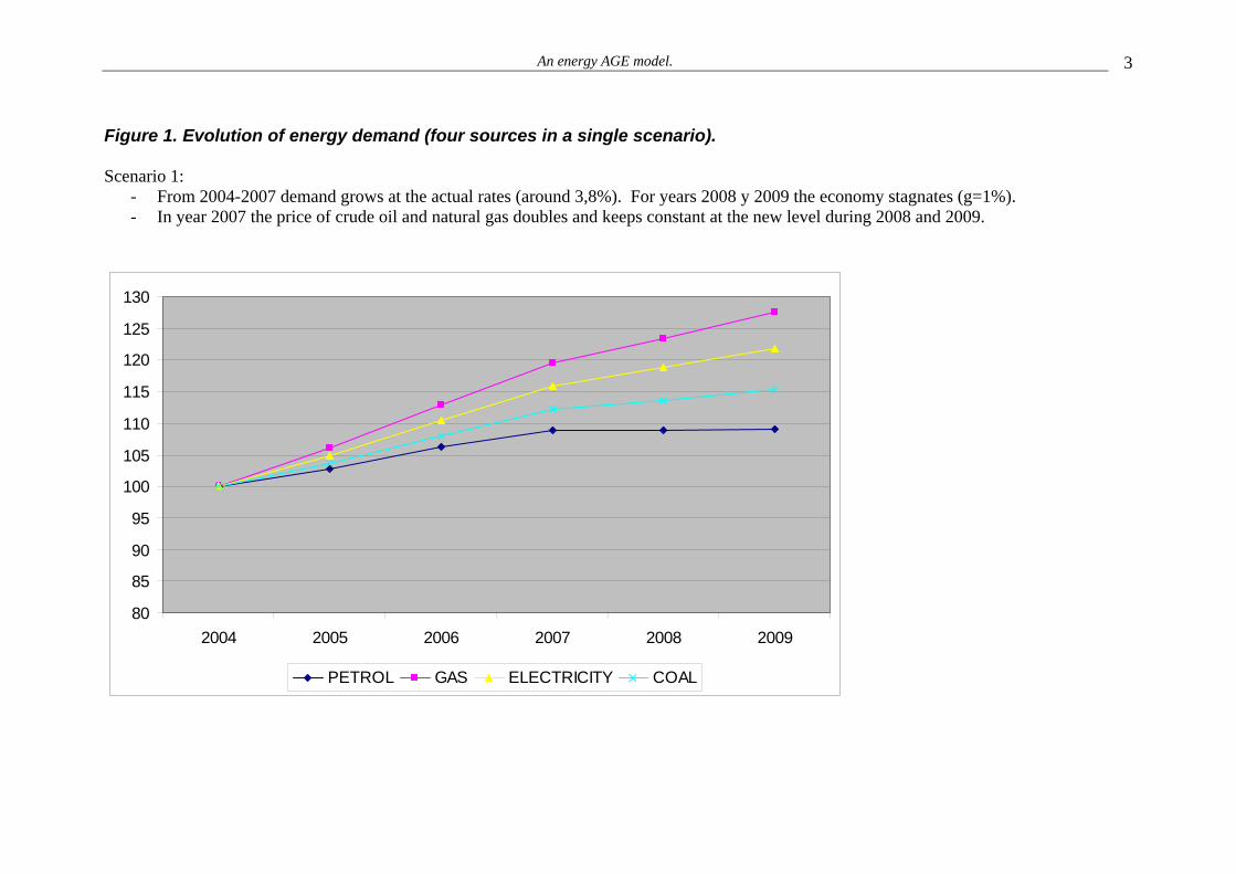
Figure 1 shows the impact on the demand for the four sources of energy

associated to the following scenario. In scenario 1 the economy grows at the

actual rates registered during years 2004 till 2007 (around 3,8%). We expect

that in 2008 and 2009 the economy will enter in recession and the rate of

growth will be reduced to 1%. Prior to 2007 the international prices of crude oil

and natural gas kept rather constant. By 2007-08 the Euro price doubled. We

expect that it will keep constant at this level during 2008 and 2009. Figure 1

graphs the results given by our mathematical model. We observe that the

demand of all products rises steadily during the first period (2004-07) due to the

high rate of growth. When the economy stagnates the demand for petrol

becomes flat. 1% of economic growth is just enough to math for the declining

petrol coefficients; the negative secular tendency of petrol is accentuated when

the prices of crude double. On the contrary, gas demand continues to increase

during the recession although at a moderate rate; the reason being that the

secular tendencies of gas coefficients are positive and rather high. Electricity

and coal occupy a intermediate position.

Figure 1

Figure 2 shows the impact on the demand for refined petrol, associated

to three alternative scenarios. Scenario 1 coincides with the one we have

contemplated in figure 1.

Scenario 2 is an optimistic one. It considers the same prices changes as

in figure 1 but assumes that the economy will be fully recovered in 2007.

During 2008 and 2009 the expected rate of growth will be 2,7%. The impact on

petrol demand would be minimum because price elasticity is quite low.


Scenario 3 is a gloomy one. Price had doubled by 2007 and double

again during this year. The impact of prices would be more important now. We

further assume that as a consequence of the higher price of petrol the economy

enters into a deep recession (g=0). The result would be a significant fall in

petrol demand. (If the result is similar in other countries, oil producing countries

could not maintain the new prices for long).

Figure 2

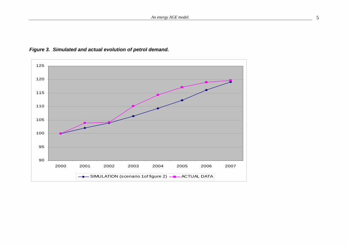
How much can we rely on the previsions of our energy AGE model? To

answer this important question we can apply the model to a period for which we

already know the true data. In our previous simulations, we had actual data for

the first part of the period 2004-07. In figure 3 we graph the data of petrol

demand provided by Spanish CNE for these years. We compare these data

with the results of our model. We verify that the adjustment is quite good. The

model predicts the general trend and most of the changes.

Figure 3

7. Conclusions.

Our energy AGE model can be summarized in two relationships: the quantity

system and the price system, both are somehow linked through technical

change.

The key determinant of energy is economic growth that reaches energy

demand through energy multipliers. They are the corner stone of the quantity

system. Technical change is the second determinant of energy demand.

Energy coefficients show a secular tendency that can be computed via

calibration and econometric methods. The secular rate of change of energy

coefficients may be speeded up or slowed down when there is a significant

change in relative prices. Technical progress constitutes the vehicle that

transmits the impact of prices changes into quantities.


How important are the impact on energy demand associated to changes

in aggregate demand, technical progress and price changes? In our analysis of

the Spanish economy we have reached the following conclusions. (1) In

general, energy coefficients tend to decline. The exception is gas, whose

coefficients continue to grow because gas is replacing petrol in many industries

and households. (2) The rate of decline of energy coefficients goes faster in

industries than in households. The exception is coal. (3) Gas and petrol are

clear substitutes; the cross elasticity between them is significant. Gas and coal

are also close substitutes in the production of electricity. In both cases the

cross elasticity is positive; in the remaining cases cross elasticities are non

significant or require time to materialize. (4) Own price elasticities are low and

they are only significant for households. (5) Income and product elasticities are

important. They justify a model like ours which relies on technical coefficients

and propensities.

Apart from the interest of empirical results, our paper has proved that it is

possible to build an energy AGE model, simple enough to be computed with

official data and to be run with an ordinary spreadsheet. The goodness of the

adjustment between forecasted and actual trends has proved to be quite good.


REFERENCES

Alcántara, V. & Padilla, E. (2003): “Key Sectors in Final Energy Consumption:

an Input-Output Application to the Spanish case”, Energy Policy, 31(5): 1673-1678.

André, F.; Cardenete, M.; Velázquez, E. (2005): “Performing an Environmental Tax Reform in a Regional Economy. A Computable General Equilibrium Approach”, Annals of Regional Science, 39 (2): 375-392

Arellano, M. (2003): “Modelling Optimal Instrumental Variables for Dynamic Panel Data Models”, Working Paper 2003_0310, CEMFI, Madrid.

Bayar, Ali (ed): Energy and Environmental Modeling, EcoMod Press, Florence, MA, 2007.

Brody, A. (1970): Proportions, Prices and Planning, Amsterdam: North Holland, Capros, A. et al (1996): “First Results of a General Equilibrium Model Linking

the EU-12 Countries”. In Carraro, C. y Siniscalo, D. (eds.): Environmental Fiscal Reform and Unemployment, Dordrecht, Kluwer, pp. 193-228.

Casler, S. & Willbur, S (1984): “Energy Input-Output Analysis. A Simple Guide”, Resources and Energy, 6: 187-201.

Dejuán, O.; Cadarso, M.A. & Córcoles, C. (1994): “Multiplicadores input-output kaleckianos: una estimación a partir de la tabla input-output española de 1990”, Economía Industrial, 298:129-144.

Dejuán, O. & Febrero, E. (2000): “Measuring Productivity from Vertically Integrated Sectors”, Economic Systems Research, 12 (1): 65-82.

Dejuán, O. (2006): “A Dynamic AGE Model from a Classical-Keynesian-Schumpeterian Approach”, Salvadori, N. (ed): Economic Growth and Distribution: on the Nature and Causes of the Wealth of Nations, Edward Elgar, Cheltenham, UK., pp. 272-291.

Dejuán, O. (2007): “A model for forecasting energy demand in Spain”, in Bayer, A. 8ed): Energy and Environmental Modeling, chapter 15, EcoMod Press, 2007, Florence, MA.

Dejuán, O. et al. (2008): Modelo de previsión de la demanda de productos derivados del petróleo en España, Trabajo presentado a la Comisión Nacional de la Energía, Madrid.

Duchin, F. (1998): Structural Economics: Measuring Change in Technology, Lifestyles, and the Environment, Washington, Island Press,

Ferguson, L.; McGregor, P.; Swales, J; Turner, K.; Yin, Y. (2005): “Incorporating Sustainability Indicators into a Computable General Equilibrium Model of the Scottish Economy”, Economic Systems Research, 17 (2): 103-140.

Galli, R. (1998): “The Relationship Between Energy Intensity and Income Levels: Forecasting long-term Energy Demand in Asian Emerging Economies”, The Energy Journal, 19 (4): 85-105.

Gately, D. y Huntington, H.D. (2002): “The Asymmetric Effects of Changes in Prices and Income on Energy and Oil Demand”, The Energy Journal, 23 (1): 19-55.

Gibson, B. & Seventer, D. van (2000): “A Tale of Two Models: Comparing Structuralist and Neoclassical Computable General Equilibrium Models for South Africa”, International Review of Applied Economics, 14 (2).


Ginsburgh, V. & Keyzer, M (2002): The Structure of Applied General Equilibrium Models, Cambridge, MA, The MIT Press.

Grubb, M.; Köhler, J. & Anderson, D. (2002): “Induced Technical Change in Energy and Environmental Modelling: Analytic Approaches and Policy Implications”, Annual Review of Energy and Environment, 27: 271-308.

Hanley, N.; McGregor, P.; Swales, K; Turner, K. (2006): “The Impact of a Stimulus to Energy Efficiency on the Economy and the Environment. A Regional Computable General Equilibrium Analysis”, Renewable Energy¸ 31 (2): 161-171.

Harvey, A.C. (1989): Forecasting Structural Time Series Models and the Kalman Filter, Cambridge, Cambridge University Press.

Herendeen, R. (1978): “Total Energy Cost of Household Consumption in

Norway, 1973”, Energy, 3: 615-630. Hoekstra, R. (2005): Economic Growth, Material Flows and the Environment,

Cheltenham, Edward Elgar. IEA (International Energy Agency) (2003): Energy Prices and Taxes, Paris,

OECD. IEA (2006 a), Energy Balances of OECD Countries, 2003-2004, Paris, OECD. IEA (2006 b): World Energy Outlook, Paris, OECD. IEA (2007): “World Energy Model Methodology and Assumptions”. Available at:

www.worldenergyoutlook.org/docs/annex_c.pdf. Judson, R.A., Schmalensee, R. y Stoker, T. M. (1999): “Economic Development

and the Structure of the Demand for Commercial Energy”, The Energy Journal, 20 (2): 29-57.

Kehoe, P. & Kehoe, T. (1994): “A Primer on AGE Models”¸ Federal Reserve Bank of Minneapolis Quarterly Review, 18 (2): 2-16. (Available in http://www.minneapolisfed.org).

Kehoe, T. Srinivasan, T. & Whalley, J. (eds) (2004): Frontiers in Applied General Equilibrium Modelling, Cambridge, Cambridge University Press.

Keynes, J.M. (1936): The General Theory of Employment, Interest and Money, London, Mcmillan.

Kurz, H.D.(1985): “Effective Demand in a ‘Classical’ Model of Value and Distribution: the Multiplier in a Sraffian Framework”, Manchester School of Economic and Social Studies, 53 (2): 121-37.

Kydes, A.S., Shaw, S.h. & McDonald, D.F. (1995): “Beyond the Horizon: Recent Directions in Long-Term Energy Modelling”, Energy, 20 (2),131-149.

Labandeira, X., Labeaga, J.M. y Rodríguez, M. (2006): “A Residential Energy Demand System for Spain”, The Energy Journal, 27 (2): 87-111.

Lenzen, M. (2006): “A Comparative Multivariate Analysis of Household Energy Requirements in Australia, Brazil, Denmark, India and Japan”, Energy, 31: 181-207.

Manresa, A.; Sancho, F. & Vegara, J.M. (1998): “Measuring Commodities’s Commodity Content”, Economic Systems Research, 10 (4): 357-365.

McKibbin, W.J. y Wilcoxen, P.J. (1993): “The Global Consequences of Regional Environmental Policies: an Integrated Macroeconomic, Multisectoral Approach”. In Kaya, Y., Nakicenovic, N. Nordhaus, W.D. y Toth, F.L. (eds.): Costs, Impacts and Benefits of CO2 Mitigation, Luxemburg, Austria, IIASA, pp. 161-178.


Miyazawa, K. & Masegi, S. (1963): “Interindustry Analysis and the Structure of Income Distribution”, Metroeconomica, 15 (2-3): 161-95.

Olatubi, W.O. y Zhang, Y. (2003): “A Dynamic Estimation of Total Energy Demand for the Southern States”, The Review of Regional Studies, 33 (2): 206-228.

Pyatt, G. & Round, J. (eds.)(1985): Social Accounting Matrices. A basis for Planning, Washington, DC. The World Bank.

Ricardo, D. (1824/1951): The Principles of Political Economy and Taxation, Cambridge, Cambridge University Press.

Roca, J. & Alcántara, V. (2002): “Economic Growth, Energy Use and CO2 Emissions”; in Blackwood, J.R. (ed): Energy Research at the Cutting Edge, New York, Novascience, pp. 123-134.

Roca, J. & Serrano, M. (2007): “Income Growth and Atmospheric Pollution in Spain: An Input-Output Approach”, Ecological Economics, pp. 230-242

Sekerka, B. Kyn, O. & Hejl, L. (1998): “Price Systems Computable from Input-Output Coefficients”, in Kurz, H.D., Dietzenbacher, E. & Lager, C: Input-Output Analysis, vol. III, pp. 223-243, Cheltenham, UK, E. Elgar.

Sraffa, P. (1960): Production of Commodities by Means of Commodities. Prelude to a Critique of Economic Theory, Cambridge, Cambridge University Press.

Sun, J.W. (1998): “Changes in Energy Consumption and Energy Intensity: a Complete Decomposition Model”, Energy Economics, 20: 85-100.

Vringer, K. & Blok, K. (1995): “The Direct and Indirect Energy Requirements of Households in the Netherlands”, Energy Policy, 23 (10), 893-910.

Welsch, H. & Ehrenheim, V. (2004): “Environmental Fiscal Reform in Germany: a Computable General Equilibrium Analysis”, Environmental Economics & Policy Studies, 6 (3): 197-219.

Young, PC.; Pedregal, D.J. & Tych, W. (1999): “Dynamic Harmonic Regression”, Journal of Forecasting, 18: 369-394.

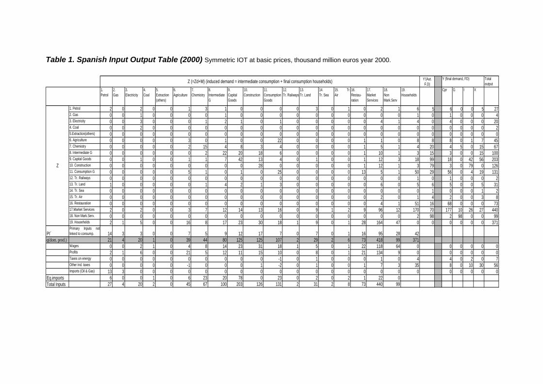
Table 1. Spanish Input Output Table (2000) Symmetric IOT at basic prices, thousand million euros year 2000.

Y’(Aut. F.D)

Total output

1. Petrol

2. Gas

3. Electricity

4. Coal

5. Extraction (others)

6. Agriculture

7. Chemistry

8. Intermediate G

9. Capital Goods

10. Construction

11. Consumption Goods

12. Tr. Railways

13. Tr. Land

14. Tr. Sea

15. Tr.Air

16. Restau- ration

17. Market Services

18. Non Mark.Serv

19. Households

Cpr G I X

1. Petrol 2 0 2 0 0 1 3 1 0 0 0 0 3 0 1 0 2 1 6 5 6 0 0 5 272. Gas 0 0 1 0 0 0 0 1 0 0 0 0 0 0 0 0 0 0 1 0 1 0 0 0 43. Electricity 0 0 3 0 0 0 1 2 1 0 1 0 0 0 0 0 4 1 4 0 4 0 0 0 204. Coal 0 0 2 0 0 0 0 0 0 0 0 0 0 0 0 0 0 0 0 0 0 0 0 0 25.Extraction(others) 0 0 0 0 0 0 0 0 0 0 0 0 0 0 0 0 0 0 0 0 0 0 0 0 06. Agriculture 0 0 0 0 0 3 0 1 0 0 22 0 0 0 0 1 1 0 8 8 8 0 1 7 457. Chemistry 0 0 0 0 0 2 15 4 8 3 4 0 0 0 0 1 5 1 4 20 4 5 0 15 678. Intermediate G 0 0 0 0 0 0 2 22 20 18 6 0 0 0 0 1 10 1 3 15 3 0 0 15 1009. Capital Goods 0 0 1 0 0 1 1 7 42 13 4 0 1 0 0 1 12 3 18 99 18 0 42 56 20310. Construction 0 0 0 0 0 0 0 0 0 28 0 0 0 0 0 1 12 1 3 79 3 0 79 0 12611. Consumption G 0 0 0 0 0 5 1 0 1 0 25 0 0 0 0 13 5 1 50 29 56 0 4 19 13112. Tr. Railways 0 0 0 0 0 0 0 0 0 0 0 0 0 0 0 0 0 0 1 0 1 0 0 0 213. Tr. Land 1 0 0 0 0 0 1 4 2 1 3 0 0 0 0 0 6 0 5 6 5 0 0 5 3114. Tr. Sea 0 0 0 0 0 0 0 0 0 0 0 0 0 0 0 0 0 0 0 1 0 0 0 1 215. Tr. Air 0 0 0 0 0 0 0 0 0 0 0 0 0 0 0 0 2 0 1 4 2 0 0 3 816. Restauration 0 0 0 0 0 0 0 0 0 0 0 0 0 0 0 0 4 1 51 16 68 0 0 0 7317.Market Services 2 0 2 0 0 3 7 12 14 13 16 0 9 1 2 9 96 12 170 70 177 10 26 27 44018. Non Mark.Serv. 0 0 0 0 0 0 0 0 0 0 0 0 0 0 0 0 0 0 2 98 2 98 0 0 9919. Households 2 1 5 0 0 16 8 17 23 30 18 1 9 0 1 28 164 47 0 0 0 0 0 0 371

PI´Primary Inputs notlinked to consump. 14 3 3 0 0 7 5 9 12 17 7 0 7 0 1 16 95 28 42

q(dom. prod.) 21 4 20 1 0 39 44 80 125 125 107 2 29 2 6 73 418 99 371Wages 0 0 2 1 0 4 8 14 23 31 18 1 5 0 1 22 118 64 0 0 0 0 0 0Profits 2 1 6 0 0 21 5 12 11 15 10 0 8 0 1 21 134 9 0 0 0 0 0 0Taxes on energy 0 0 0 0 0 0 0 0 0 0 -1 0 1 0 0 0 1 0 4 4 0 2 0 7Other ind. taxes 0 0 0 0 0 -1 0 0 0 1 -2 0 1 0 0 1 7 3 35 8 0 10 30 56Imports (Oil & Gas) 13 3 0 0 0 0 0 0 0 0 0 0 0 0 0 0 0 0 0 0 0 0 0 0

Eq.imports 6 0 0 1 0 6 23 20 78 0 23 0 2 0 2 1 22 0Total Inputs 27 4 20 2 0 45 67 100 203 126 131 2 31 2 8 73 440 99

Z

Z (=Zd+M) (induced demand = intermediate consumption + final consumption households) Y (final demand, FD)


Table 2. Energy multipliers.

Me 2004 1. Petrol 2. Gas 3. Electricity 4. Coal 5.Extraction (others) 6. Agriculture 7. Chemistry

8. Intermediate

Goods

9. Capital Goods

10. Construction

11. Consump-tion Goods

12. Tr. Railways 13. Tr. Land 14. Tr. Sea 15. Tr. Air 16.

Restauration17.Market Services

18. Non Mark.Serv.

19. Households

1. Petrol 1,0823 0,0089 0,0813 0,0650 0,0866 0,0416 0,0631 0,0340 0,0227 0,0305 0,0304 0,0425 0,0704 0,0819 0,1311 0,0334 0,0306 0,0311 0,03932. Gas 0,0044 1,0026 0,0537 0,0116 0,0317 0,0087 0,0153 0,0200 0,0094 0,0098 0,0114 0,0118 0,0081 0,0077 0,0059 0,0095 0,0096 0,0102 0,01093. Electricity 0,0290 0,0140 1,2333 0,1157 0,0776 0,0470 0,0482 0,0685 0,0459 0,0439 0,0498 0,1203 0,0507 0,0473 0,0280 0,0438 0,0503 0,0511 0,05044. Coal 0,0021 0,0007 0,0596 1,0060 0,0040 0,0025 0,0026 0,0051 0,0026 0,0026 0,0027 0,0061 0,0027 0,0025 0,0016 0,0024 0,0027 0,0029 0,0027

Me 20091. Petrol 1,0843 0,0074 0,0783 0,0645 0,0893 0,0377 0,0586 0,0305 0,0201 0,0272 0,0270 0,0390 0,0616 0,0725 0,1211 0,0290 0,0266 0,0269 0,03342. Gas 0,0048 1,0029 0,0580 0,0128 0,0344 0,0097 0,0171 0,0223 0,0106 0,0109 0,0127 0,0136 0,0091 0,0087 0,0065 0,0106 0,0108 0,0115 0,01193. Electricity 0,0296 0,0142 1,2341 0,1172 0,0796 0,0496 0,0523 0,0749 0,0498 0,0467 0,0535 0,1353 0,0546 0,0510 0,0291 0,0463 0,0539 0,0548 0,05094. Coal 0,0020 0,0007 0,0568 1,0058 0,0039 0,0025 0,0026 0,0052 0,0027 0,0026 0,0027 0,0065 0,0027 0,0025 0,0015 0,0024 0,0027 0,0029 0,0026 Note: Me of year 2009 takes into account the evolution of energy coefficients (secular trends and impact of price elasticity) from 2000 to 2009. (We suppose that oil and gas prices double in 2007 and keep constant at the new level) Table 3. Price impact when the Euro price of crude oil and natural gas doubles.

1. Petrol 2. Gas 3. Electricity 4. Coal 5.Extraction (others) 6. Agriculture 7. Chemistry

8. Intermediate

Goods

9. Capital Goods

10. Construction

11. Consump-tion Goods

12. Tr. Railways 13. Tr. Land 14. Tr. Sea 15. Tr. Air 16.

Restauration17.Market Services

18. Non Mark.Serv.

19. Households

1,6702 1,6911 1,1368 1,0461 1,0877 1,0482 1,0559 1,0376 1,0177 1,0213 1,0290 1,0307 1,0750 1,0757 1,0968 1,0282 1,0259 1,0164 1,0344


Table 4. Secular tendencies of energy coefficients (τ).

1. Petrol 0,02 0 -0,01 -0,028 -0,0252. Gas 0,015 0,02 0,015 0,03 0,023. Electricity 0 0,025 0,03 0,03 -0,0354. Coal -0,01 0 0 0 -0,051

Other Services HouseholdsEnergy Other

Industries Transport

Table 5. Price elasticities of energy demand (ε) (after a 100% change in prices)

1. Petrol 0 -0,042. Gas 0 -0,013. Electricity 0 -0,014. Coal 0 0

Industry Households


Figure 1. Evolution of energy demand (four sources in a single scenario). Scenario 1:

- From 2004-2007 demand grows at the actual rates (around 3,8%). For years 2008 y 2009 the economy stagnates (g=1%). - In year 2007 the price of crude oil and natural gas doubles and keeps constant at the new level during 2008 and 2009.

80

85

90

95

100

105

110

115

120

125

130

2004 2005 2006 2007 2008 2009

PETROL GAS ELECTRICITY COAL


Figure 2. Evolution of the demand for petrol in three different scenarios. Scenario 1: As the previous one (figure 1). g=1% in 2008, 2009 Scenario 2 (an optimistic one). In 2008 and 2009 demand grows at 2,7%. Constant prices after the increase in 2007. Scenario 3 (a pessimistic one). The prices of crude oil and natural gas had doubled by 2007 and double again in 2007. As a consequence the economy experience a deep recession (g=0).

90

95

100

105

110

115

2004 2005 2006 2007 2008 2009

SCENARIO 1 SCENARIO 2 SCENARIO 3


Figure 3. Simulated and actual evolution of petrol demand.

90

95

100

105

110

115

120

125

2000 2001 2002 2003 2004 2005 2006 2007

SIMULATION (scenario 1of figure 2) ACTUAL DATA

An energy AGE model. Forecasting energy demand in Spain

Documents

Transcript of An energy AGE model. Forecasting energy demand in Spain