An empirical study of stock portfolios based on

diversification and innovative measures of risks.

Master Thesis - Final Report

Supervised by Pr. Dr. Sornette

Chair of Entrepreneurial Risks at ETH Zurich

Thibaut Simon

10 February 2010

Abstract

When a measure of risks such as variance does not take into account the fact thatdistribution of returns are non-Gaussian and exhibit non-linear dependencies,it is ineffective to generate portfolios with standard optimization procedures.This study proposes to explore new measures of risks based on series and newconcepts of level of risks. This empirical study back-tests these innovative ideason the long run and evaluates them with random portfolios analyses. Persis-tent performance and risk management are achieved with the use of MaximumDrawDown of returns and levels of diversification.

Contents

1 Introduction 3

2 Classical approach of Portfolio construction 52.1 Markowitz, Mean-Variance . . . . . . . . . . . . . . . . . . . . . 52.2 Different estimates of the Covariance matrix to improve Mean-

Variance approach . . . . . . . . . . . . . . . . . . . . . . . . . . 82.2.1 Shrinkage . . . . . . . . . . . . . . . . . . . . . . . . . . . 82.2.2 Re-sampling . . . . . . . . . . . . . . . . . . . . . . . . . . 82.2.3 Reverse engineering . . . . . . . . . . . . . . . . . . . . . 8

2.3 CAPM and extensions . . . . . . . . . . . . . . . . . . . . . . . . 9

3 Genetic algorithm 123.1 Composition . . . . . . . . . . . . . . . . . . . . . . . . . . . . . 123.2 Focus on the generation of a new population . . . . . . . . . . . 143.3 Applications . . . . . . . . . . . . . . . . . . . . . . . . . . . . . . 17

4 Random Portfolios 184.1 First attempt . . . . . . . . . . . . . . . . . . . . . . . . . . . . . 184.2 Second attempt . . . . . . . . . . . . . . . . . . . . . . . . . . . . 204.3 Conclusion . . . . . . . . . . . . . . . . . . . . . . . . . . . . . . 22

5 Innovative idea on risks 235.1 Measures of risks and dependencies . . . . . . . . . . . . . . . . . 23

5.1.1 Coherent Measure of risk . . . . . . . . . . . . . . . . . . 235.1.2 Dependencies . . . . . . . . . . . . . . . . . . . . . . . . . 245.1.3 Some measure of risks . . . . . . . . . . . . . . . . . . . . 24

5.2 Level of risks and diversification . . . . . . . . . . . . . . . . . . 255.3 A winner mix . . . . . . . . . . . . . . . . . . . . . . . . . . . . . 28

6 Simulation 306.1 Methodology . . . . . . . . . . . . . . . . . . . . . . . . . . . . . 30

6.1.1 Data . . . . . . . . . . . . . . . . . . . . . . . . . . . . . . 306.1.2 Test . . . . . . . . . . . . . . . . . . . . . . . . . . . . . . 316.1.3 Set of strategies . . . . . . . . . . . . . . . . . . . . . . . . 32

1

6.2 Results . . . . . . . . . . . . . . . . . . . . . . . . . . . . . . . . . 356.2.1 Tables . . . . . . . . . . . . . . . . . . . . . . . . . . . . . 356.2.2 Wealth evolution - first interpretation . . . . . . . . . . . 376.2.3 Random Portfolios - Luck or skill? . . . . . . . . . . . . . 436.2.4 Sharpe Ratio . . . . . . . . . . . . . . . . . . . . . . . . . 536.2.5 Transaction costs overview . . . . . . . . . . . . . . . . . 596.2.6 Impact of the diversification - concrete cases . . . . . . . 63

7 What’s next? 667.1 Recommendation . . . . . . . . . . . . . . . . . . . . . . . . . . . 667.2 To go further . . . . . . . . . . . . . . . . . . . . . . . . . . . . . 67

8 Annexes 758.1 Maximum DrawDown - Matlab Code . . . . . . . . . . . . . . . . 758.2 Average Maximum DrawDown - Matlab Code . . . . . . . . . . . 76

2

Chapter 1

Introduction

Asset allocation is today a topic of real importance. All investors want toinvest in the winning combination of assets. This combination should give themthe maximum level of return for the level of risk they are able to take. Theproblematic of asset allocation can be found across all industries and sectorsof activity. For example, an oil company will have the choice of investing indifferent fields with different techniques for different products. How to choosethe weight each project should have in my investment portfolio? Answering thisquestion requires to take into account expected returns of projects as well asrisks of failure, or delay that could penalize future returns. Actually, investingin several assets means trade-offs. However, making a decision is hard becauseinvestors have no idea about what will happen and what the consequences oftheir choice will be? Thus the idea of portfolio optimization is to develop adecision-tool to help investors to rationalize their choice.

A lot of researches have been done in the area of asset allocation and portfoliooptimization and construction. However, the topic is still widely open. Why isit still the case? Harry Markowitz created the modern portfolio theory basedon historical distributions of returns considered to be Gaussian. As describedin my thesis, this theory never performed well. However, the Markowitz’ ideaof minimizing risks for a given level of return is still widely accepted as a goodstart for a new theory. In the 1950’s means of computation were limited butMarkowitz developed a quadratic programming equation that could be easilysolvable. Today new measures of risks and dependencies between assets can beused, since computation and optimization of complex problem is more conve-nient. These new measures allow to create new strategies that perform betterthan the traditional one. I use a genetic algorithm (see chapter 3) to solve op-timization problems. The performance of these strategies is evaluated throughrandom portfolios and Sharpe ratio analyses. This study covers stock portfo-lios taken in a universe composed of 28 stocks from the CAC40. The questionanswered in my thesis is:

3

How to achieve persistent return for different levels of risks?

This report will help people to start from scratch in portfolio managementand optimization to understand the problematic of portfolio construction andevaluation. Hence, this thesis will start by explaining the classical approach, itslimits and extensions before describing the method and tools to construct andevaluate portfolios. From the development of random portfolios emerges theinnovative idea of separating measures of risks and levels of risks. It is testedin the chapter presenting the simulation. My thesis ends with some insight andway to continue it.

4

Chapter 2

Classical approach ofPortfolio construction

Portfolio construction aim at producing portfolios minimizing risks for in-vestors and maximizing their wealth. Portfolios are constructed from a basisof selected assets. Determining the universe of stocks that seems interesting toget in a portfolio is done by financial analyst. Hence a basic set of stocks isproduced, the question is: how to weight each of these assets? That is whatis about portfolio theory. Keep in mind, that a good theory, should producewell diversified portfolio, to decrease risks and volatility of the portfolio. How-ever it should still be able to increase wealth of investors more than a randomallocation could. This chapter is about the state of the art on the traditionalapproach of investment.

2.1 Markowitz, Mean-Variance

Harry Markovitz is considered as the father of modern portfolio theory [16].He developed during the 50’s a theory based on the assumption that the utilityfunction of investors is quadratic. This theory tells that investors want to mini-mize their risks for a given level or return. In this quadratic framework the riskis modelled by the standard deviation of the portfolio. At this time this wasa good model, because this problem has an analytical solution which allowedpeople to use it with the small computation means of this age.

This approach never gave fully satisfaction, due to a lack of empirical evi-dence. In practice some limitations have been identified: returns don’t follow anormal distribution and samples are too noisy to provide good Covariance esti-mates. Different solutions emerged to improve covariance’s estimates. I presentthree of them in the following section.

5

Minimize wTVw

Subject to :

wTµ = r0∀i, wi ≥ 0n∑

i=1

wi = 1

Where:

• w : portfolio weights

• V : covariance matrix

• r0 : the desired level of expected return of the portfolio

• µ : vector of expected returns

Figure 2.1: Formulation of Mean-Variance optimization

Figure 2.2: Instability of the EFFICIENT FRONTIER moving at each periods.Efficient frontiers from 28 assets over 12 periods of 6 months.

6

Figure 2.3: DEVIATION of a portfolio from the EFFICIENT FRONTIER.Same frontiers as figure 2.2 with the evolution of a portfolio taken on the firstefficient frontier. A portfolio done in the Mean-Variance frameworks becomerapidly inefficient.

7

2.2 Different estimates of the Covariance matrixto improve Mean-Variance approach

Covariance matrix can be estimate with the sample covariance matrix. How-ever this simple estimator does not work much for portfolio construction, sincesamples are not sufficiently big and are to noisy to give a good estimate. Ac-tually, sample covariance estimates are really sensitive to outliers. Neverthelessthis estimator is unbiased.

2.2.1 Shrinkage

The shrinkage method allows to provide a better estimation of the covariancematrix when the number of assets p is bigger than the size of the sample n. Inthe case p > n, the sample covariance matrix become singular. The shrinkagemethod is an alternative. It consists to evaluate through a cross validation,the shrinking parameter. The shrinking parameter is the weight determiningthe trade-off between the sample covariance estimator and the diagonal targetmatrix. This operation regularizes the covariance matrix.

S = kT F + (1− k

T )S

• k : estimator of the optimal shrinkage constant

• T : number of observations

• F : single index covariance matrix

• S : sample covariance matrix

Figure 2.4: SHRINKAGE Method - a trade off between sample covariance andsingle index

2.2.2 Re-sampling

The idea is to expand sample by creating samples from the original sample.This method is well known in statistics under the name of bootstrap method.It allows to reduce the variance uncertainty while increasing the bias on themeasure. However this technique seems to give some results, if we believe M.Michaud who is the developer of this technique to portfolios construction. Ac-cording to him, the re-sampling decrease the sensitivity of optimization to noise.

2.2.3 Reverse engineering

This method consists in assuming that the market portfolio is on the efficientfrontier. The aim is to correct the covariance matrix estimate with the help of

8

the market efficient portfolio. This idea is theoretically pleasant. However ithas a lack of empirical use, since market portfolio is hard to estimate.

Figure 2.5: REVERSE ENGINEERING - Measure of distance from the sampleto the reverse engineering estimate. The factor alpha corresponds to the trade-off between the bias and the variance of our estimation

Figure 2.6: REVERSE ENGINEERING - Minimizing the distance of the reverseengineering estimate to the sample estimate under the condition that the marketefficient portfolio belows to the efficient frontier

2.3 CAPM and extensions

Capital Asset Pricing Model Sharpe, Lintner and Mossin developed theCAPM theory in the 60’s [18]. This model complements the Markovitz portfoliotheory by adding the possibility to lend or borrow money at a risk free rate.Main assumptions are taken from the Markovitz portfolio theory: agents are riskaverse and maximize their utility, stocks returns are normally distributed, per-fect markets, informational efficiency, supply and demand equilibrium. It givesa clear relation between risk and return. The Capital Asset Pricing Model takesinto account two risks: the unique risk which can be cancelled by diversification,and the market risk which corresponds to the risk of being on the market. Theexpected risk premium on stock is equal to r−rf where rf is the risk free rate of

9

return and r the expected return of the stock. Sharpe established the followingrelationship between risk and return:

r − rf = β(rm − rf )

Beta represents the contribution of the market risk to the non-diversifiable stockrisk. Beta is the relative covariance of stock to market returns. Beta measuresthe dependence between the stock and the market, weighted by the ratio of thestock volatility by the market volatility.

βi = Cov(ri,rm)V ar(rm)

This model is linear, so easily understandable. However this theory is not fullyuseful since the market portfolio can only be approximate ( Roll critique [17]).These critics lead researchers to improve this model.

3-factors model based on size of firms and book-to-value Eugene Famaand Kenneth French extended the CAPM model by adding two new factors: firmsize and the book-to-market equity [12]. With this improvement, the model be-comes multi-linear. The cross-section of expected returns is better explainedwith this theory. However this model is built on empirical study and the mech-anisms are not deeply understood.

Our preliminary work on economic fundamentals suggests that high-BE/ME1 firms tend to be persistently poor earners relative to low-BE/ME firms. Similarly, small firms have a long period of poorearnings during the 1980s not shared with big firms. The systematicpatterns in fundamentals give us some hope that size and book-to-market equity proxy for risk factors in returns, related to relativeearning prospects, that are rationally priced in expected returns. [12]

4-factors model based on momentum strategies This model developedby John Cahart aims at taking into consideration the effect of time when pricingstocks. [8] Researchers detected a momentum effect from data. Momentumstrategies are founded on empirical and behavioural finance. They benefit froman inefficiency of the market, with a lag generated by investors. Stocks with thehighest return remain good choice for about 6 months, and the opposite withlow returns stocks[13, 1]. The fact of adding a one year momentum in stocksreturns improves the prediction power of the model.

”First, note the relatively high variance of the SMB2 , HML3, andPR1YR4 zero-investment portfolios and their low correlations witheach other and the market proxies. This suggests the 4-factor model

1ME refers to size of the firm. It is equal to the market value. BE refers to the book valueof the firm. BE/ME is called the book-to market equity.

2factor of size3factor of book-to-market equity4factor referring to the one year momentum in stock returns.

10

can explain sizeable time-series variation.” ”I find that the 4-factormodel substantially improves on the average pricing errors of theCAPM and the 3-factor model”[8]

2-factors model based on market concentration This model has beendeveloped by Malevergne, Santa-Clara and Sornette in their papers ProfessorZipf goes to Wall Street (2009)[15]. It is based on the Zipf distribution offirm size. The idea is that the market portfolio is concentrated into very fewcompanies (about 20) due to the heavy-tailed shape of the Zipf distribution.This market concentration can be measured with the Herfindahl Index, thatwill be used widely in the following sections. This concentration leads to anew factor of systematic risk. The difference between the equally weighted andvalue-weighted market portfolios is used as a proxy of the Zipf factor, and allowsto take this new risk into account in the pricing model. This idea of marketconcentration influenced my work.

Application of these models These models are used to evaluate the perfor-mance of investment strategies. The idea is to compare the average returns ofthe portfolio against portfolios sharing the same factors. Then, it remains thequestion of the persistence of these results. Are managers lucky or truly skilled?[11]. This question is fundamental. The random portfolio theory of P. Burns,is preferred in the following for portfolios performance evaluation.

11

Chapter 3

Genetic algorithm

Genetic algorithm allows to optimize all kinds of functions. Genetic algo-rithms are part of evolutionary algorithm [14, 9]. They directly come from theDarwin’s theory of evolution. This algorithm reproduces the selection processworking in the nature. Generation after generation, the population adapts it-self to the environment. In the case of a stable environment, GA produces anoptimization solver which converges. The evolution of the population is donethrough small change coming from the mix of parents or through mutation. Itis really convenient to use, once parameters that regularize performance of theoptimization, are understood. Its name and the associated vocable come fromgenetics. The process of reproduction is actually a model of what is going on inour cells. The genotype is evolved across generations through selection, cross-over and mutation processes, which converge to a final population answeringthe problem. I use this algorithm to do the final simulation of this study.

3.1 Composition

The genetic algorithm is composed of 4 main steps :

1. initialisation of the population

2. evaluation of the population

3. selection

4. reproduction

The steps 2,3 and 4 are in a loop which stops when a stopping criteria is reached.The reproduction step is composed of three possibilities:

1. elite count

2. crossover

3. mutation

12

Figure 3.1 represents the reproduction process.

Below is published the description of the genetic algorithm used in my work.This algorithm exists already in the GA toolbox of Matlab. Here are the optionsand properties used to do optimization of portfolio. In order to obtain theattending result, it is good to understand, how each function works, and tohave a global view of the process.

Population Options:

Population is composed of portfolios represented as vectors of weights.

Population size specifies how many individuals there are in each genera-tion. With a large population size, the genetic algorithm searches thesolution space more thoroughly, thereby reducing the chance that thealgorithm will return a local minimum that is not a global minimum.Here you can choose between 100 and 1000.

Initial population specifies an initial population for the genetic algo-rithm. It is set as random with the constraint : ∀i, 0 ≤ wi. Theother constraint of normality is taken into account in the evaluationfunction.It is not an optimization constraint, because the answer ofthe problem is a vector representing the proportion of the differentassets. Hence the portfolio is normalized, only during the evaluationof the portfolio. At the end, the final vector of weights is normalizedto further use. This astuteness avoids to use constraint options ofthe GA toolbox. It saves computation time.

Evaluation function: The evaluation function quantifies the objective of theoptimization. It allows to rank portfolios in function of the distance tothe solution of the optimization problem. These ranks are used in theselection process.

Selection function: It allows to select parents for reproduction. The Stochas-tic uniform selection function lays out a line in which each parent corre-sponds to a section of the line of length proportional to its scaled value.The algorithm moves along the line in steps of equal size. At each step,the algorithm allocates a parent from the section it lands on. The firststep is a uniform random number less than the step size.

Reproduction:

Crossover fraction specifies the fraction of the next generation otherthan elite children, which are produced by crossover.

Elite count specifies the number of individuals that are guaranteed tosurvive to the next generation.

13

Mutation uses the Gaussian mutation function, which adds a randomnumber taken from a Gaussian distribution with mean 0 to eachentry of the parent vector.

Crossover uses the scattered crossover function, which creates a randombinary vector and selects the genes where the vector is a 1 from thefirst parent, and the genes where the vector is a 0 from the secondparent, and combines the genes to form the child.

Stopping Criteria Options: The algorithm runs until the cumulative changein the fitness function value over Stall generations is less than or equal toFunction Tolerance. Here the number of generation is limited to 200 andstall limit generation can be chosen between 10 and 50.

3.2 Focus on the generation of a new population

The process of the generation of the new population is composed of threeoperations: direct transfer from the old to the new generation, mix of two par-ents and mutation of one guy. Figure 3.1 explains the process and gives theventilation between the three operations. Parameters of the algorithm deter-mine its performance feature. Large population (over 300) produces a resultmore pertinent in less generations, but increase the computation. Moreover asmall crossover rate increases the number of mutation and the chance to findlocal minimum. However the convergence of the population will become slowerand slower. The crossover decreases the variance of the population by makingchromosome more and more identical(figure 3.2). The crossover operation lookfor global minimum. In opposition, the mutation operation, which add somerandom change in the population, tend to diversify the population. In the algo-rithm that I used in this study, the Gaussian mutation function adds a randomnumber taken from a Gaussian distribution with mean 0 to each entry of theparent vector(figure 3.3). This operation helps in the convergence process tofind the local minimum.

14

Figure 3.1: REPRODUCTION PROCESS using elite count, crossover and mu-tation. In this example the crossover rate is 0.8 and the elite count is 2

Figure 3.2: A view of the scattered CROSSOVER function process. A randomvector of bit is generated of the length equal the number of assets in the portfolio.A zero means we select the weight of parent 1 and a one the weight of parent 2

15

Figure 3.3: Gaussian MUTATION function adds a random number taken froma Gaussian distribution with mean 0 to each entry of the parent vector.

16

3.3 Applications

With a good parametrization this algorithm performs well in optimizationof portfolios. First, this GA will be used to construct portfolios following astrategy. In this case, the population is a population of random portfolios.These random portfolios will be generation after generation evolved until theyoptimized the fitness function. The fitness function is the objective functiondescribing the investment strategies. For instance, a strategy could be to reducethe variance of portfolios returns while keeping a diversification of 10 stocks. Allthe condition have to be integrate in the objective function (diversification,...).The second use of this algorithm, is the creation of set of random portfolios.Since the initial population and the search process are random, the GA allowsto create such random portfolios meeting the needed constraints. These twoapplications are used for simulation in this study.

17

Chapter 4

Random Portfolios

Introduction Random portfolios technique is about statistical simulation ofportfolios. Random portfolios constitute a benchmark. This benchmark canbe used to evaluate other portfolios. Papers [7, 6] explain how to use thistechnique for testing trading strategies, assessing the skill exhibited by funds,and implementing investment mandates. Random Portfolios are an applicationof Monte Carlo simulation. The result of a random portfolios simulation is thepossibility to rank a portfolio against random ones. The main difficulty of this,is to compare what is comparable. In this sense, the way random portfolios aregenerated is of terrible importance. The first section of this chapter is a naiveapproach of random portfolios. I explain why it does not work. The secondsection presents a good procedure to obtain results from random portfolios. Ichoose to present this party in a narrative way to present the dynamic of myapproach.

Hypothesis Random portfolios are used as a statistical test. The hypothesisdefining the p-value are:

H0: Strategy is not better than random portfolios

H1: Strategy is better than random portfolios

Hence a p-value of ten percent means that the strategy performs better than 90percents of random portfolios.

4.1 First attempt

Use of the function random I generated random portfolios from the sim-plest method I knew : the function random. Each weight is assigned to a randomdouble between 0 and 1. Then the portfolio vector is normalized to respond tothe constraint: sum of weights equal to 1. I generated 1000 portfolios. ThenI applied them to a period of 6 months of data returns. I obtain a Gaussian

18

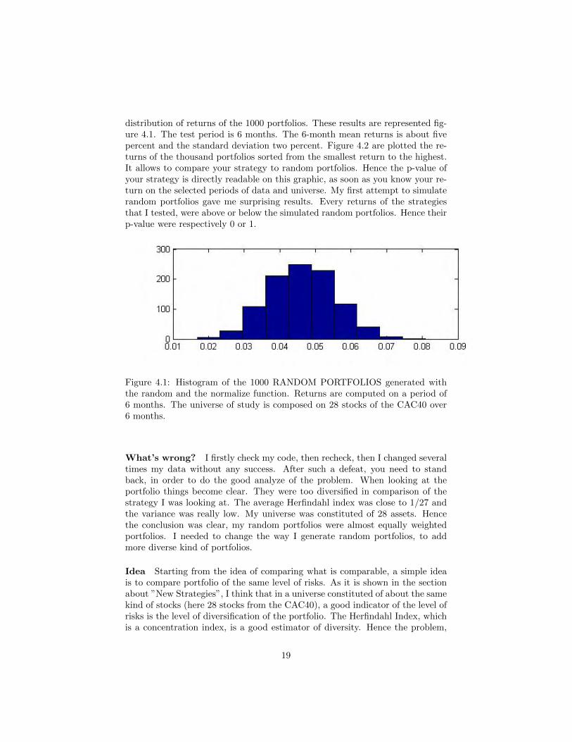
distribution of returns of the 1000 portfolios. These results are represented fig-ure 4.1. The test period is 6 months. The 6-month mean returns is about fivepercent and the standard deviation two percent. Figure 4.2 are plotted the re-turns of the thousand portfolios sorted from the smallest return to the highest.It allows to compare your strategy to random portfolios. Hence the p-value ofyour strategy is directly readable on this graphic, as soon as you know your re-turn on the selected periods of data and universe. My first attempt to simulaterandom portfolios gave me surprising results. Every returns of the strategiesthat I tested, were above or below the simulated random portfolios. Hence theirp-value were respectively 0 or 1.

Figure 4.1: Histogram of the 1000 RANDOM PORTFOLIOS generated withthe random and the normalize function. Returns are computed on a period of6 months. The universe of study is composed on 28 stocks of the CAC40 over6 months.

What’s wrong? I firstly check my code, then recheck, then I changed severaltimes my data without any success. After such a defeat, you need to standback, in order to do the good analyze of the problem. When looking at theportfolio things become clear. They were too diversified in comparison of thestrategy I was looking at. The average Herfindahl index was close to 1/27 andthe variance was really low. My universe was constituted of 28 assets. Hencethe conclusion was clear, my random portfolios were almost equally weightedportfolios. I needed to change the way I generate random portfolios, to addmore diverse kind of portfolios.

Idea Starting from the idea of comparing what is comparable, a simple ideais to compare portfolio of the same level of risks. As it is shown in the sectionabout ”New Strategies”, I think that in a universe constituted of about the samekind of stocks (here 28 stocks from the CAC40), a good indicator of the level ofrisks is the level of diversification of the portfolio. The Herfindahl Index, whichis a concentration index, is a good estimator of diversity. Hence the problem,

19

Figure 4.2: Graphics of RANDOM PORTFOLIOS sorted by increasing returns.The 1000 random portfolios were generated with the random and the normalizefunction. Returns are computed on a period of 6 months. The universe of studyis composed on 28 stocks of the CAC40 over 6 months..

is to generate random portfolios of the same Herfindahl index as the studiedportfolio. This could not be done using only the random function.

4.2 Second attempt

Using the Genetic Algorithm The second attempt consisted in creatingrandom portfolios with a constrained level of diversification. The Genetic Al-gorithm(GA) developed and parametrized to do portfolio optimization revealeditself a good way of creating random portfolios. The fitness function of the GAhas to be equal to the constraint |Σw2

i − Hportfolio|. Then the GA select arandom portfolio which satisfies to the constraint of the level of diversification.Hence the GA has to be ran thousand times to create the population of thou-sand random portfolios. It is a computationally time consuming to do, but itgives the expected result. 1

Result of the experience Figure 4.3 and 4.4 you can observe that the newrepartition of random portfolios in term of returns is wider. The range of returnsis now from - 20 percent et + 30 percent. Now the calculated p-value are between0 and 1. The evaluation of strategies is possible. The p-value represent the rankin percentage of the strategy against the random portfolios. However one p-valuefor one period is not enough to decide whether the strategy is good or whetherthe result is due to luck.

1A computationally cheaper way to generate random portfolios with a Herfindahl Con-straint is to use hyper-spherical coordinate

20

Figure 4.3: Histogram of the 1000 RANDOM PORTFOLIOS generated with aGenetic Algorithm at a Herfindahl Index of 1/3. Same period and universe asfigure 4.1. We can observe that the range of returns is much wider than this offigure 4.1

Figure 4.4: Graphics of RANDOM PORTFOLIOS sorted by increasing returns.The 1000 random portfolios were generated with a Genetic Algorithm at aHerfindahl Index of 1/3. Same period and universe as figure 4.2. This graphicscan be used to read the p-value of your strategy on this particular period anduniverse if its herfindahl index is 1/3.

21

4.3 Conclusion

Random Portfolios technique should be used carefully. Always remind thissentence of good sense: compare what is comparable. Figure 4.5 represent p-values for different Herfindahl index value. Random portfolios are specific of auniverse. Based on a same level of risks, the use of random portfolios and p-value is a really powerful tool to assess the performance of a strategy. Howeverthis evaluation should be done over a significant amount of periods of time toensure the validity of the result against luck. The use of statistic to createinterval of confidence around the mean p-value observed should give insight onthe fundamental question skilled or not? One idea to increase the validity ofthe p-value test would be to cut a big period on different scales. For example,cutting a period of 6 months in 60 periods of 3 months to compute more p-values. However this cut could have an impact on the pertinence of result byuncorrelating the test and the strategy studied.

Figure 4.5: RANDOM PORTFOLIOS return for different level of the HerfindahlIndex. Each line corresponds to a different p-value. The universe of portfoliosis composed of 28 stocks of the CAC40. Six months of daily returns are used toevaluate portfolios returns. Thousand random portfolios were generated with aGenetic Algorithm for the 28 levels of the Herfindahl index ( 1,1/2,1/3...1/28)

22

Chapter 5

Innovative idea on risks

The creation of new strategies should be based on new measure of risks. Theuse of the variance or standard deviation as a measure of risks could not anymore agreed as valid by researchers. The general idea of investment strategyshould still minimize risks and maximize returns of the portfolio. Computa-tion is not any more a problem with computer of today. The use of geneticalgorithm allows strategies based on non-linear measures of risks. With thegenetic algorithm, there is no need for a n-th improvement of the estimationof the covariance matrix, because optimization problems don’t need to be ex-posed under a quadratic form to be solve. My innovative idea is to separate themeasure of risks to be minimized and the level of risks taken. The level of risksrepresents the profile of risk wanted by investors. The measure of risks will giveinformation to select stocks in a safe way.

5.1 Measures of risks and dependencies

5.1.1 Coherent Measure of risk

In the paper ”Coherent Measure of risk” [2], the authors develop a theoryexplaining what properties should have a good measure of risk in portfolio man-agement.

”A risk measure satisfying the four axioms of translation invariance,subadditivity, positive homogeneity and monotonicity is called co-herent.” [2]

Translation invariance If a ∈ R and X ∈ L then ρ(a + X) ≤ ρ(X) − aThe value a is just adding cash to your portfolio X, which acts like aninsurance: the risk of X + a is less than the risk of Z, and the difference isexactly the added cash a. In particular, if a = ρ(Z) then ρ(Z+ρ(Z)) = 0.

Sub-additivity If X1, X2 ∈ L, then ρ(X1 + X2) ≤ ρ(X1) + ρ(X2)The risk of two portfolios together cannot get any worse than adding

23

the two risks separately: this is the diversification principle.

Positive homogeneity If α ≥ 0 and X ∈ L then ρ(αX) = αρ(X)Loosely speaking, if you double your portfolio then you double your risk.

Monotonicity If X1, X2 ∈ L and X1 ≤ X2, then ρ(X1) ≤ ρ(X2)That is, if portfolio X2 has better values than portfolio X1 under allscenarios then the risk of X2 should be bigger than the risk of X1: moreprofit, more risk.

5.1.2 Dependencies

Measures of risks are correlated to the universe of the study. Dependenciesare included in the measure of risks. Properties of dependencies depend onthe measure of risks used. For example, minimizing the variance of a portfoliois not the same as minimizing the weighted some of variances of single assetscorresponding to the same portfolio, because variance is non-linear (actually,it is quadratic). Minimizing a measure of risks on a whole portfolio takes intoconsideration the dependencies between assets. This compensation ,betweenassets of a portfolio, has a positive impact on the property of the portfolio, ifthe measure of risks is coherent. Hence dependencies are taken into account.

5.1.3 Some measure of risks

Below are listed some measure of risks and their main interests. These mea-sures are used in the section Simulation, to create portfolio. They are all wellknown, except the Maximum DrawDown of returns for which I think to bethe creator. ”If Maximum DrawDown of stock prices is the speed, MaximumDrawdown of returns is the acceleration.”

Variance: That is the most commonly used measure of risk in portfolio opti-mization. It is convenient to calculate and represent. One problem of thevariance is that extreme risks are not taken into account.

Moment of even higher order (4,6,8): Moment of order 4, 6, 8 takes intoaccount extreme risks. They indeed characterize fat-tailed distribution.

Maximum DrawDown of stock price: The maximum loss from peak to val-ley. The Maximum DrawDown has some nice property. It is invariant bytranslation , it is homogeneous and convex. Thus the MDD is a coherentmeasure as the volatility.

Average Maximum DrawDown of stock price: It takes the average fromthe Maximum DrawDown of a time-series of stock prices. See the code ofthe function in annexe

Maximum DrawDown of returns: Like the Maximum DrawDown of stockprices, but based on the series of returns. In comparison with physics,

24

Figure 5.1: Illustration of two MAXIMUM DRAWDOWNS

it represents the extreme acceleration of the system. As it will be shownin the part simulation, the MDD of returns performs well in portfoliooptimization.

Value at Risk: The VaR measures the loss of a portfolio for a given quantile.It is currently controversial since it does not take into account extremerisks. Moreover this measure is not coherent for a non-Gaussian distribu-tion.

Conditional Value at Risk: the second name of C-VaR is the expected short-fall. This measure is known as a coherent measure of risks. It benefitsfrom the criticism of the VaR. It is more sensitive to the shape of the lossdistribution. Extreme risks are taken into account, because it focuses onworst scenario quantiles.

Semi-variance: This risk measure aims at measuring the variance for the neg-ative returns. The logic is that variance of positive returns is an opportu-nity, but variance of negative returns represents a risk.

Deviation to the median: This risk measure is a kind of standard deviation.It takes into account the asymmetry of the distribution of returns.

5.2 Level of risks and diversification

Introduction Risks are often associated with diversification. Using coher-ent measure of risks implies that risks is diminishing with diversification (sub-additivity property). A portfolio containing stocks of one company, will looseeverything if the company die. However if the portfolio contains stocks of twocompanies in equal proportion, and one company dies, the portfolio will stillhave the value from the other company.

25

An easy example to understand the impact of diversification

Given A and B two independent companies,P(A=1) the probability that the company A survives until next year,P(A=0) the probability that the company A dies before next year,

the value of the company remains equal to 1 during the year in case of survival,the value of the company remains equal to 0 in case of death,

Π1 the portfolio containing only stocks of A for a total value of 100Π2 the portfolio containing stocks A and B in equal proportion for a totalvalue of 100

P(A=1)=P(B=1)=0,99P(A=0)=P(B=0)=0,01

The expected value of portfolios at the end of the year is the same in both case:E(Π1) = 100× (1× P (A = 1) + 0× P (A = 0)) = 0, 99E(Π2) = 50× (1× P (A = 1) + 0× P (A = 0)) + 50× (1× P (B =1) + 0× P (B = 0)) = 0, 99E(Π1) = E(Π2)

However, the extreme risk that the portfolio is equal to 0 is:P (Π1 = 0) = P (A = 0) = 0.01P (Π2 = 0) = P (A ∩B = 0) = P (A = 0)× P (B = 0) = 0.0001

This example shows a reduction by hundred of the risk of loosing everything.Note that for non-independent companies, P (A∩B = 0) = P (A = 0)×P (B = 0)is not valuable any-more. However the result P (Π2 = 0) ≤ P (Π1 = 0) is stilltrue. In conclusion, diversification gives benefit in lowering extreme risks.

Herfindahl Index The Herfindahl index is a measure of diversification. Itis used in economics, to study the concentration of a market. If it’s value isclose to zero, it means that the market shares are distributed among a lot ofcompanies. In opposition, if it’s value is close to one, the market share areconcentrated in few companies.This indicator allows to select the number ofcompanies wanted in your portfolio during the process of optimisation. Forinstance, if you want about 5 different assets under the assumption of equallyweighted portfolio, H =

∑5i=0 w

2i = 1

5 . As it is shown in the figure 5.2, therisks is decreasing with the increase of the diversification of portfolios. In thisexample, the minimum return of simulated portfolios goes from -17 percent to2 percent when the average number of stocks in portfolios goes from 28 to 1.The same is true of the maximum return of the portfolios. Over the period, it isdivided by 6 from 30 percent to 5 percent. Small Herfindahl Index implies smallrange of variation and lower risks. Moreover the Herfindahl index is quite stablewith the evolution of a portfolio. As you can see on figure 5.3, variations of the

26

Herfindahl index are not significant over a period of 122 days of evolution. It istrue with other value of the Herfindahl index and other period of time.

To be short, ”High degree of diversification implies small range of performanceavailable. Low degree of diversification implies high range of performance

available”

Figure 5.2: ENVELOP of returns taken by 1000 random portfolios calculatedfor H0 = [1, 1/2 1/3, 1/4, 1/5, ..., 1/28] over a period of 121 days. H0 is thevalue of the Herfindahl Index the first day of the period.

27

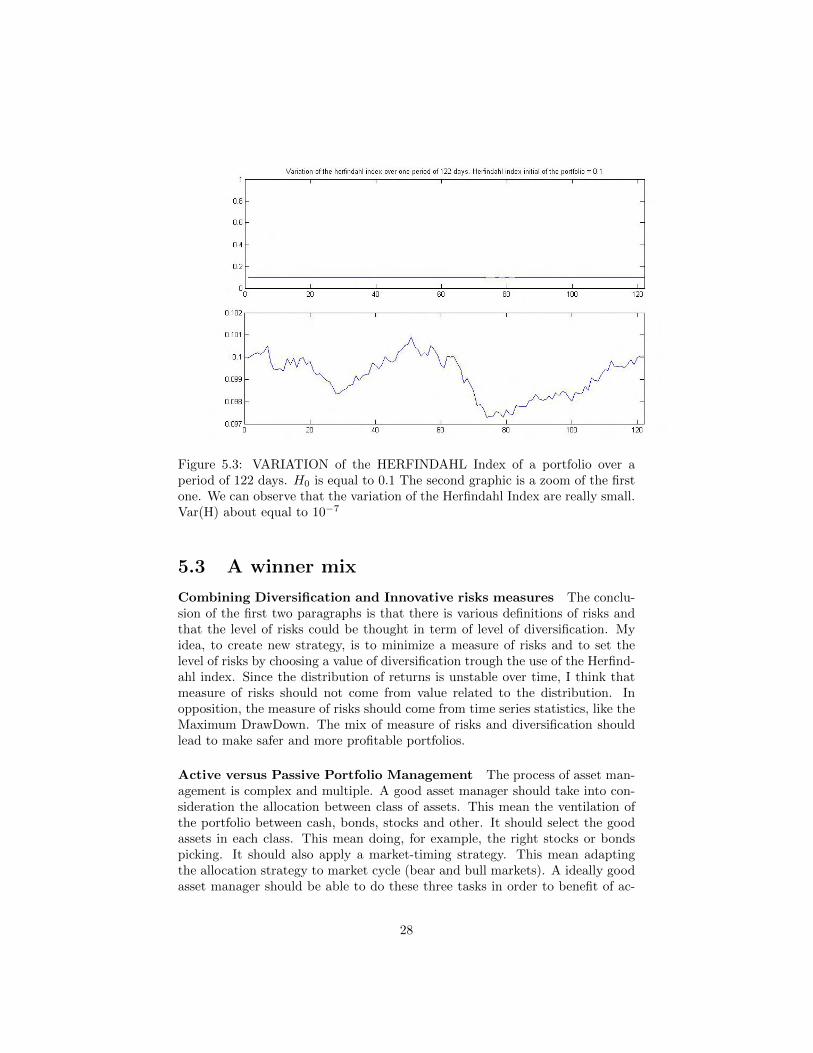
Figure 5.3: VARIATION of the HERFINDAHL Index of a portfolio over aperiod of 122 days. H0 is equal to 0.1 The second graphic is a zoom of the firstone. We can observe that the variation of the Herfindahl Index are really small.Var(H) about equal to 10−7

5.3 A winner mix

Combining Diversification and Innovative risks measures The conclu-sion of the first two paragraphs is that there is various definitions of risks andthat the level of risks could be thought in term of level of diversification. Myidea, to create new strategy, is to minimize a measure of risks and to set thelevel of risks by choosing a value of diversification trough the use of the Herfind-ahl index. Since the distribution of returns is unstable over time, I think thatmeasure of risks should not come from value related to the distribution. Inopposition, the measure of risks should come from time series statistics, like theMaximum DrawDown. The mix of measure of risks and diversification shouldlead to make safer and more profitable portfolios.

Active versus Passive Portfolio Management The process of asset man-agement is complex and multiple. A good asset manager should take into con-sideration the allocation between class of assets. This mean the ventilation ofthe portfolio between cash, bonds, stocks and other. It should select the goodassets in each class. This mean doing, for example, the right stocks or bondspicking. It should also apply a market-timing strategy. This mean adaptingthe allocation strategy to market cycle (bear and bull markets). A ideally goodasset manager should be able to do these three tasks in order to benefit of ac-

28

tive or dynamic portfolio management. A lot of studies show that funds don’tbeat the market [11]. Hence the question of active management versus passivemanagement become pertinent. In the following, I choose to study a light activemanagement: adjustment of the portfolio every 6 months.

29

Chapter 6

Simulation

Aim of the simulation This simulation looks at the impact of new measureof risks in portfolio construction. The main question is: Is it possible to createnew allocation strategies, for a given level of risks, that give persistent andconsistent results? I developed for the purpose of this study, an optimizationtool and an analysis tool to perform this simulation, using Matlab and a geneticalgorithm. Moreover the analysis of performance will estimate the p-values fromrandom portfolios analysis, to compare the different strategies.

6.1 Methodology

6.1.1 Data

Stocks returns The data used in this simulation are 28 stocks of the CAC40 from the 17/01/2003 to the 03/08/2009. Data come from the website YahooFinance. Returns on stocks are calculated from daily adjusted-closing prices.The adjusted-closing price takes into account changes due to dividend and splitof the stock price. The large number of stocks has been chosen to create realisticportfolios. You can observe figure 6.1, the evolution of the CAC 40 during theperiod used. It corresponds to the end of the 2001 crisis, followed by the sub-prime bubble, the crash of the stocks market in 2008, followed by the increaseof 2009.

Survival and Look-ahead Bias In empirical finance, results can be biaseddue to a survival effect coming from the selection of the data. The survivalbias corresponds to the fact, that simulation is done from data of stocks whichare still alive. Hence it forgot enterprise that died during the time set of thesimulation. It has been shown that the survival bias could increase return of astrategy during a simulation [5, 10]. I choose only 28 assets from the CAC40instead of 40. Is my study subject to survival bias? First, no enterprise of theCAC40 died during the time of the simulation. Enterprise of the CAC40 are

30

Figure 6.1: Evolution of the CAC40.

generally big enough to survive. However some enterprises disappear due tomergers and acquisition (GDF-Suez), or appear due to new regulation for ex-ample Suez environment detached from Suez or GDF detached from EDF. It didnot increase the survival bias since these enterprises are not under-performingor over-performing the market. Second I did not include every assets due toa lack of quality of certain data where the adjusted price was not taking intoaccount split. In conclusion I think that my data are not impacted a lot bysurvival bias. Concerning the look-ahead bias, my procedure of test will use aperiod to create the portfolio, which will be test on the period after. Since Idid not use future information in the past, my study should not be impactedby this bias (see figure 6.2). However it is necessary to be introduced to thelook-ahead benchmark bias which appears in case of benchmark comparison.It comes from the fact that the constitution of the benchmark is permanentlyevolving and that the information of this constitution is not easily available andusable. [10]

6.1.2 Test

Strategy The main idea of this simulation is to test the idea of level of risksbased on the Herfindahl index for investment in stocks in a limited universe. Thestrategies of investment will take into account a constraint of diversification anda measure of risks that will be minimized. All these strategies will be comparedto the equally weighted portfolio. This will provide a base of comparison. Thestrategies will be back tested with the data described below. The portfolioswill be constructed from the last year of data and kept during the 6 following

31

Periods Training data Test datafrom to from to

period 1 17/01/2003 16/01/2004 19/01/2004 02/07/2004period 2 04/07/2003 02/07/2004 05/07/2004 17/12/2004period 3 19/12/2003 17/12/2004 20/12/2004 03/06/2005period 4 04/06/2004 03/06/2005 06/06/2005 18/11/2005period 5 19/11/2004 18/11/2005 21/11/2005 05/05/2006period 6 06/05/2005 05/05/2005 08/05/2006 20/10/2006period 7 21/10/2005 20/10/2006 23/10/2006 06/04/2007period 8 07/04/2007 06/04/2007 09/04/2007 21/09/2007period 9 22/09/2006 21/09/2007 24/09/2007 07/03/2008period 10 09/03/2007 07/03/2008 10/03/2008 22/08/2008period 11 24/08/2007 22/08/2008 25/08/2008 11/02/2009period 12 11/02/2008 11/02/2009 12/02/2009 03/08/2009

Figure 6.2: This table contains the different PERIODS OF DATA used duringthe simulation. Training data are the data used to create a portfolio. Test dataare the data used to evaluate the portfolio. Training data contained 260 daysand test data 120 days.

months.

Optimization The optimization will be realized with a tool developed inMatlab, using a genetic algorithm. The optimization tool cut the data intoperiods on which it performs in serial the optimization of all the strategies. Theresult of this optimisation is stored in one file to be analysed next. It containsthe portfolio selected for the next 6-months period and data of this test periodin order to enable the analysis later on.

Evaluation of performance The analysis is done by an other tool developedin Matlab. It allows to look at each of the strategies for each sub-period andto compare them. It proceeds to the evaluation of transaction costs, of thewealth, of the evolution of the strategies over all the periods. Moreover randomportfolios p-values and Sharpe ratios of strategies will be estimated from testdata at each sub-period.

6.1.3 Set of strategies

Here are the different sets of strategies analysed. The optimal portfolio for theperiod will be calculated by the optimization software on the precedent period.w represents the vector of portfolio’s weights of dimension n the number ofassets. R represents the matrix of returns n ×m with n the number of assetsand m the number of trading days of the period. V represents the matrix ofstocks’ price.

32

w∗ optimal portfolio such as F (R.w∗) +Hc(w∗) is minimum with F the riskmeasure and Hc the diversification constraint. No short selling is allowed:

∀i, 0 ≤ wi ≤ 1. The other constraint on weights is:n∑

i=1

wi = 1.

Minimum Variance Strategy

1. min var(R.w) + |1− h(w)|2. min var(R.w) + | 12 − h(w)|3. min var(R.w) + | 13 − h(w)|4. min var(R.w) + | 14 − h(w)|5. min var(R.w) + | 15 − h(w)|6. min var(R.w) + | 16 − h(w)|7. min var(R.w) + | 17 − h(w)|8. min var(R.w) + | 18 − h(w)|9. min var(R.w) + | 19 − h(w)|

10. min var(R.w) + | 110 − h(w)|11. min var(R.w)

12. min | 128 − h(w)|

Minimum Moment of order 4 Strategy

1. min µ4(R.w) + |1− h(w)|2. min µ4(R.w) + | 12 − h(w)|3. min µ4(R.w) + | 13 − h(w)|4. min µ4(R.w) + | 14 − h(w)|5. min µ4(R.w) + | 15 − h(w)|6. min µ4(R.w) + | 16 − h(w)|7. min µ4(R.w) + | 17 − h(w)|8. min µ4(R.w) + | 18 − h(w)|9. min µ4(R.w) + | 19 − h(w)|

10. min µ4(R.w) + | 110 − h(w)|11. min µ4(R.w)

12. min | 128 − h(w)|

Minimum Maximum DrawDown of returns Strategy

1. min MDD(R.w) + |1− h(w)|2. min MDD(R.w) + | 12 − h(w)|3. min MDD(R.w) + | 13 − h(w)|

33

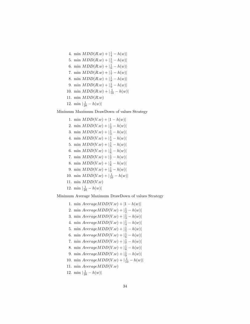
4. min MDD(R.w) + | 14 − h(w)|5. min MDD(R.w) + | 15 − h(w)|6. min MDD(R.w) + | 16 − h(w)|7. min MDD(R.w) + | 17 − h(w)|8. min MDD(R.w) + | 18 − h(w)|9. min MDD(R.w) + | 19 − h(w)|

10. min MDD(R.w) + | 110 − h(w)|11. min MDD(R.w)

12. min | 128 − h(w)|

Minimum Maximum DrawDown of values Strategy

1. min MDD(V.w) + |1− h(w)|2. min MDD(V.w) + | 12 − h(w)|3. min MDD(V.w) + | 13 − h(w)|4. min MDD(V.w) + | 14 − h(w)|5. min MDD(V.w) + | 15 − h(w)|6. min MDD(V.w) + | 16 − h(w)|7. min MDD(V.w) + | 17 − h(w)|8. min MDD(V.w) + | 18 − h(w)|9. min MDD(V.w) + | 19 − h(w)|

10. min MDD(V.w) + | 110 − h(w)|11. min MDD(V.w)

12. min | 128 − h(w)|

Minimum Average Maximum DrawDown of values Strategy

1. min AverageMDD(V.w) + |1− h(w)|2. min AverageMDD(V.w) + | 12 − h(w)|3. min AverageMDD(V.w) + | 13 − h(w)|4. min AverageMDD(V.w) + | 14 − h(w)|5. min AverageMDD(V.w) + | 15 − h(w)|6. min AverageMDD(V.w) + | 16 − h(w)|7. min AverageMDD(V.w) + | 17 − h(w)|8. min AverageMDD(V.w) + | 18 − h(w)|9. min AverageMDD(V.w) + | 19 − h(w)|

10. min AverageMDD(V.w) + | 110 − h(w)|11. min AverageMDD(V.w)

12. min | 128 − h(w)|

34

6.2 Results

6.2.1 Tables

These tables represent indicators resulting from the simulation. The datawere subset in 12 test periods from the 19/01/2004 to the 03/08/2009. Newportfolios are generated at each sub-period.

Herfindahl 1 12

13

14

15

16

17

18

19

110 free 1

28

Variance 180 175 140 251 127 101 126 141 107 105 133 112µ4 221 123 150 122 87,8 125 114 124 89 85 131 112

MDD(r) 231 141 141 123 146 150 133 144 139 137 129 112MDD(v) 139 205 174 128 133 134 130 128 122 120 134 112

A-MDD(v) 95 115 122 98 127 109 118 127 119 108 116 112

Figure 6.3: END WEALTH of the different strategies at the date of 03/08/2009.Starting value of 100 the 19/01/2004.

Herfindahl 1 12

13

14

15

16

17

18

19

110 free 1

28

Variance 165 145 112 222 103 77 105 119 86 86 124 108µ4 204 93 123 92 59 99 91 101 69 65 121 108

MDD(r) 216 112 117 101 125 133 117 129 126 125 116 108MDD(v) 111 179 152 106 114 116 114 113 109 107 117 108

A-MDD(v) 64 85 98 72 105 88 99 111 103 94 100 108

Figure 6.4: END WEALTH including TRANSACTION COSTS of 1 percent ofthe total value traded. Starting value of 100 the 19/01/2004.

Herfindahl 1 12

13

14

15

16

17

18

19

110 free 1

28

Variance 0,38 0,38 0,40 0,24 0,45 0,56 0,43 0,37 0,41 0,48 0,32 0,49µ4 0,35 0,46 0,41 0,46 0,51 0,43 0,51 0,45 0,64 0,60 0,31 0,50

MDD(r) 0,36 0,45 0,38 0,41 0,38 0,35 0,37 0,36 0,35 0,36 0,34 0,50MDD(v) 0,40 0,29 0,35 0,46 0,41 0,41 0,40 0,40 0,43 0,43 0,40 0,49

A-MDD(v) 0,52 0,47 0,45 0,51 0,43 0,45 0,44 0,40 0,44 0,50 0,43 0,49

Figure 6.5: Average RANDOM PORTFOLIOS P-VALUES of the differentstrategies for the period from 19/01/2004 to 03/08/2009.

35

Herfindahl 1 12

13

14

15

16

17

18

19

110 free 1

28

Variance 0,82 0,74 0,98 1,28 0,78 0,68 0,92 1,12 1,03 0,83 1,34 0,73µ4 1,01 0,56 0,71 0,48 0,55 0,67 0,61 0,73 0,37 0,45 1,32 0,73

MDD(r) 0,85 0,60 1,12 1,01 1,25 1,27 1,16 1,23 1,20 1,21 1,24 0,73MDD(v) 0,65 1,08 1,03 0,75 1,09 1,08 1,05 1,07 0,96 0,96 0,97 0,73

A-MDD(v) 0,22 0,53 0,75 0,60 0,89 0,85 0,89 1,02 0,99 0,75 0,88 0,73

Figure 6.6: Average yearly SHARPE RATIO of the different strategies for theperiod from 19/01/2004 to 03/08/2009.

Ranks Wealth generated Sharpe ratio Random Portfolios Overall PerformanceVariance 2 3 3 3

µ4 4 5 5 5MDD(r) 1 1 1 1MDD(v) 3 2 3 3

A-MDD(v) 5 4 4 4

Figure 6.7: Result summary. Numbers represent the rank of strategies againsteach other.

36

6.2.2 Wealth evolution - first interpretation

Some stylized facts on result A first comparison of the wealth generated byeach set of strategies during the back-testing period give an idea on performance.Figure 6.3 exhibits the value of portfolios at the end of the 12 periods of thesimulation for every set of strategies. For each strategy new portfolios aregenerated at the beginning of each period based on the previous year of data.The starting value (19/01/2004) is 100. The end of the simulation is 03/08/2009.At this date, the equally weighted portfolios achieved a performance of 12.2percent. The equally weighted portfolio strategy represents the performanceof the market. It is used as a benchmark. Looking at the generated wealth,strategies based on Maximum DrawDown of returns and of values have resultsabove the equally weighted portfolios for every level of diversification simulated.These two measures of risks seem to contain above the average informationabout the capacity to grow of portfolios. Their power of prediction leads to highreturns. Moreover, figures 6.10 and 6.11 represent the evolution of their wealth.These graphics confirm the fact that portfolios based on Maximum DrawDownof returns and values perform at every level of diversification more than thebenchmark on the long run. Set of strategies based on Variance and 4th Momentdon’t give such strong robustness and persistence on results. They have highperformance with portfolios poorly diversified (1-4 stocks) and low performanceagainst the benchmark with diversified portfolios(5-10 stocks). Finally strategybased on Average Maximum DrawDown of values seem to provide no interests.

Robustness to diversification A measure of risks, which could producegood performance whatever its level of diversification, provide a good base for aninvestment strategy. It proves its capacity to predict which stocks will producehigh performance over the next period. The reliability of the measure of risksshould be proved for different configuration of portfolios. Hence the robustnessto diversification is a good indication of reliability. Figure 6.13 shows resultsof the table 6.3 under a Box plot form. Maximum DrawDown of returns boxis smaller and above the others. It means that in average its performance isabove the other strategy. Moreover its performance is robust to diversificationsince the size of the box is small. It means that strategies based on MaximumDrawDown on return provide, in the long run, high returns for every level ofdiversification. Strategy based on Variance provide more risky investment sincethe Box of results is wide. It means that this measure of risks is really sensibleto diversification. It could have low or high unexpected results. Are theseresults the fruit of luck? This question needs a random portfolios analysis tobe answered. Finally, strategies based on Average-Maximum-DrawDown onvalue produce robustness to diversification for bad returns. Its box is small, butlocated below the others with a small mean. Hence this measure should not beused (same conclusion for the 4th Moment measure of risks).

Stock picking The aim of an investment strategy in stocks is to select stocksthat produce high returns and have low volatility. Stock picking is based on

37

qualitative and quantitative analysis. The study of the different set of strate-gies shows for some measures of risks a non-robustness. However, 4th Momentand Variance strategies show extremely high return for portfolios composed of 1to 4 assets. One explanation could be luck! Nevertheless, an other explanationcould be that selecting 1 to 4 stocks over 28, require less information and com-petency than selecting 10 good stocks. This could explain the fact that Varianceand 4thMoment measures of risks could lead to select some good stocks, but notbe able to select one entire portfolio. Moreover, portfolios construct withoutconstraint of diversification (Herfindahl level free) seems to perform better andlead to portfolio of lower volatility than portfolio of equivalent degree of diver-sification. The constraint impacts negatively the level of information containedby the measure of risks.

Profile of risks In the universe of commercial finance, assets’ managers haveto care about the profile of their investors, to offer them, product adapted totheir risk acceptance. I think that based on the result of figures 6.3 and 6.13,3 profiles emerged. These profile take their sense in a fund which would use ameasure of risks robust to diversification in a small universe of large stocks likethe CAC40.

• The speculative profile composed of 1 or 2 stocks.

• The risky profile composed from 3 to 5 stocks.

• The secure profile composed by the optimisation without any constraint.

38

Figure 6.8: Wealth evolution of VARIANCE based strategies from 19/01/2004to 03/08/2009.

Figure 6.9: Wealth evolution of 4th MOMENT based strategies from 19/01/2004to 03/08/2009.

39

Figure 6.10: Wealth evolution of MAXIMUM DRAWDOWN of RETURNSbased strategies from 19/01/2004 to 03/08/2009.

Figure 6.11: Wealth evolution of MAXIMUM DRAWDOWN of VALUES basedstrategies from 19/01/2004 to 03/08/2009.

40

Figure 6.12: Wealth evolution of Average MAXIMUM DRAWDOWN of VAL-UES based strategies from 19/01/2004 to 03/08/2009.

41

Figure 6.13: Comparison of the strategies in term of WEALTH at the end of thesimulation from 19/01/2004 to 03/08/2009. All Herfindahl index mixed. Thered horizontal line represent the median. The boundaries of the box representthe 25 and 75 quantile. The whiskers represent the minimum and maximumvalues. Maximum values corresponds generally to high Hefindahl index (lookat the table 6.3 to see the corresponding values plotted here). This plot showsthat strategies based on different measures of risks have different responses todiversification.

42

6.2.3 Random Portfolios - Luck or skill?

Consistency of results Random portfolios allow to rank a strategy. In thisstudy, the p-value is calculated for each sub-strategy and each sub-period. Re-sults are plotted in graphics 6.14, 6.15, 6.16, 6.17, 6.18. It is interesting toobserve how variable is the p-value for each strategy. A consistent strategyshould have a high mean p-value and a small range of variation in order to showconsistency. On the maps plotted below the 3D graphics, dark area representslow p-value. Hence a map with a high dark coverage along the 2 axes: strategyand period; means that the measure of risks is robust to diversification and givespersistent value added during time.

4th Moment This set of strategies does not show any robustness to diversifi-cation. The median p-value is really different for each sub-strategy(levelof diversification). Box of the box-plot are big. Hence the p-value of eachsub-strategy is very different for different periods. It means that this mea-sure of risks don’t provide many information. The map seems completelyrandom implying no consistency in results.

Variances This set of strategies does not show any regularity of results. Themap seems random. However p-value are in averaged smaller than 0.5, meaning that they are performing better than the expected value ofsomeone acting randomly(see table 6.5 for the average p-values over sub-periods). Is it due to luck? Sub-strategy 4 and 11 are especially good inthis simulation.

MDD of returns This set of strategies shows a good robustness to diversifi-cation. Boxes of sub-strategies are quite similar. dark area on the mapare predominant. P-values are almost the same for each sub-strategies.The map reveals a periodicity. For example, p-values are bad for all sub-strategies at the period 10 and 12. The mean and median p-values arelow for most of the periods meaning that strategies based on MaximumDrawDown of returns provide a real plus to luck. This strategy seemsconsistent.

MDD of values This set of strategies shows a good robustness to diversifica-tion. Like the Maximum DrawDown of returns, dark area is predominantwith a periodicity of bad p-value. Median p-value is quite good (less than0.5) for all the sub-strategies but less than those of Maximum DrawDownof returns. On the boxplot graphic, sub-strategy 2 (with 2 stocks) isparticularly good. However the difference of p-value for different periodimplies a strong correlation of the performance to market condition.

Average MDD of values This set of strategies shows a kind of robustness todiversification, however the bright trend is dominant. P-values are highmeaning no skill at all. This measure of risks does not provide informationof prediction. It is not effective at selecting interesting stocks.

43

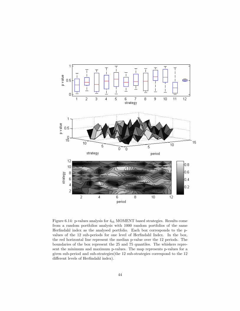
Figure 6.14: p-values analysis for 4th MOMENT based strategies. Results comefrom a random portfolios analysis with 1000 random portfolios of the sameHerfindahl index as the analysed portfolio. Each box corresponds to the p-values of the 12 sub-periods for one level of Herfindahl Index. In the box,the red horizontal line represent the median p-value over the 12 periods. Theboundaries of the box represent the 25 and 75 quantiles. The whiskers repre-sent the minimum and maximum p-values. The map represents p-values for agiven sub-period and sub-strategies(the 12 sub-strategies correspond to the 12different levels of Herfindahl index).

44

Figure 6.15: p-values analysis for VARIANCE based strategies. Results comefrom a random portfolios analysis with 1000 random portfolios of the sameHerfindahl index as the analysed portfolio. Each box corresponds to the p-values of the 12 sub-periods for one level of Herfindahl Index. In the box,the red horizontal line represent the median p-value over the 12 periods. Theboundaries of the box represent the 25 and 75 quantiles. The whiskers repre-sent the minimum and maximum p-values. The map represents p-values for agiven sub-period and sub-strategies(the 12 sub-strategies correspond to the 12different levels of Herfindahl index).

45

Figure 6.16: p-values analysis for MAXIMUM DRAWDOWN of RETURNSbased strategies. Results come from a random portfolios analysis with 1000random portfolios of the same Herfindahl index as the analysed portfolio. Eachbox corresponds to the p-values of the 12 sub-periods for one level of HerfindahlIndex. In the box, the red horizontal line represent the median p-value over the12 periods. The boundaries of the box represent the 25 and 75 quantiles. Thewhiskers represent the minimum and maximum p-values. The map represents p-values for a given sub-period and sub-strategies(the 12 sub-strategies correspondto the 12 different levels of Herfindahl index).

46

Figure 6.17: p-values analysis for MAXIMUM DRAWDOWN of VALUES basedstrategies. Results come from a random portfolios analysis with 1000 randomportfolios of the same Herfindahl index as the analysed portfolio. Each boxcorresponds to the p-values of the 12 sub-periods for one level of HerfindahlIndex. In the box, the red horizontal line represent the median p-value over the12 periods. The boundaries of the box represent the 25 and 75 quantiles. Thewhiskers represent the minimum and maximum p-values. The map represents p-values for a given sub-period and sub-strategies(the 12 sub-strategies correspondto the 12 different levels of Herfindahl index).

47

Figure 6.18: p-values analysis for AVERAGE MAXIMUM DRAWDOWN ofVALUES based strategies. Results come from a random portfolios analysis with1000 random portfolios of the same Herfindahl index as the analysed portfolio.Each box corresponds to the p-values of the 12 sub-periods for one level ofHerfindahl Index. In the box, the red horizontal line represent the median p-value over the 12 periods. The boundaries of the box represent the 25 and 75quantiles. The whiskers represent the minimum and maximum p-values. Themap represents p-values for a given sub-period and sub-strategies(the 12 sub-strategies correspond to the 12 different levels of Herfindahl index).

48

Asymmetry of performance As observed in the previous paragraph, Max-imum DrawDown of returns and values especially show a sensibility to the pe-riod in performance. Figures 6.19,6.21,6.20 represent the performance of sub-strategies against 10 percent best random portfolios (p-value of 0.1). The marketperiod 11 decreases a lot and the market period 12 increases strongly. Thesegraphics confirm the asymmetry of performance of strategy based on measureof risks, especially in the case of the Maximum DrawDown. This asymmetrycomes from the ability of these strategies to select stocks that perform the mostin bear market, but to select the ones that perform the less in extremely growingmarket. The leverage effect can be an explanation of this assymetry. This effectcorresponds to a negative correlation between past returns and future volatility[4]. Moreover minimizing a measure of risks necessary means minimizing theextreme variation. Hence these measures failed to pick stocks that will growstrongly. However this effect is interesting to create defensive strategy for bearmarket.

Remark on the equally weighted portfolio The equally weighted portfoliohas a p-value of 0.5 since there is only one equally weighted portfolio by universe.It represents a good estimator of the 0.5 p-value random portfolios for every levelof diversification. Hence the equally weighted portfolio is a good benchmark ofperformance, because it represents the expected return of a random strategy.

49

Figure 6.19: Return of strategies based on MAXIMUM DRAWDOWN of RE-TURNS, against random portfolios of p-value of 0.1 . In Period 11, the marketdecreases and in period 12, it increases

50

Figure 6.20: Return of strategies based on 4thMOMENT, against random port-folios of p-value of 0.1 In Period 11, the market decreases and in period 12, itincreases

51

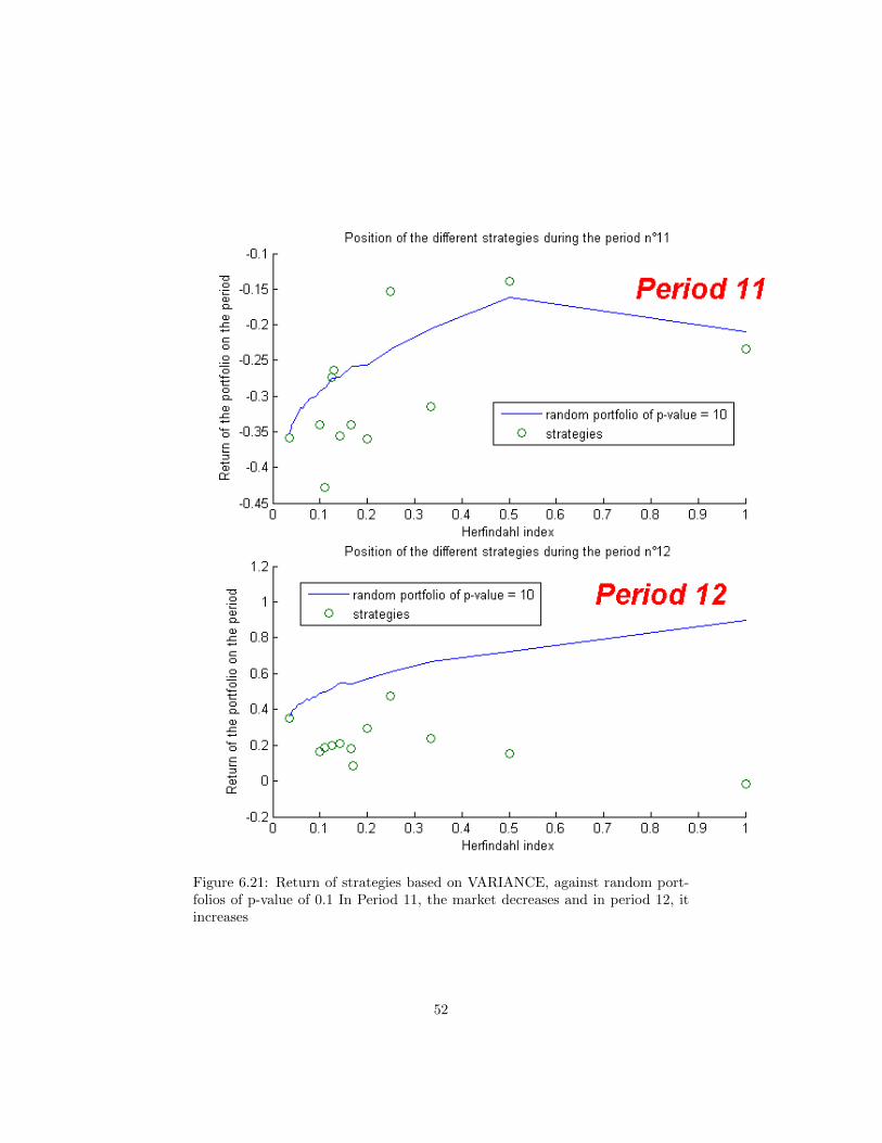
Figure 6.21: Return of strategies based on VARIANCE, against random port-folios of p-value of 0.1 In Period 11, the market decreases and in period 12, itincreases

52

6.2.4 Sharpe Ratio

The Sharpe Ratio is defined as the ratio of the mean excess-year return and theyearly standard deviation. Excess returns correspond to the series of portfolioreturns minus the risk free rate. The risk free rate of return is estimated withthe US-3-months-treasury bills. This ratio gives an information on how big isthe performance in comparison with its variability. It is a classical indicatorof performance computed in most studies. A ratio above one is considered asgood.

Analysis of the strategies The comparison of these results confirms the ex-cellent performance of portfolios based on the Maximum DrawDown of returns.These portfolios get in average a Sharpe ratio above one when they contain morethan two stocks (see table 6.6). Almost all levels of diversification give betterresult than the equi-weighted portfolio. Portfolios based on the 4th Momentgive particularly bad Sharpe ratios, often below the equi-weighted portfolio.

Surprisingly, portfolios based on Variance are not the best. This is a proofthat the measure of the one-year variance is not a good predictor to select stocksthat provide small variance. Indeed Variance portfolios generate more wealththan Maximum DrawDown of Values portfolios. When in the mean time, theaverage Sharpe ratio of Maximum DrawDown of Values portfolios is higher (seetable 6.7).

Graphics representing Sharpe ratio for sub-periods and sub-strategies showthat its value is strongly dependent on the period, and moreover on the marketperformance of the period (see figures 6.22, 6.23, 6.24, 6.25,6.26).

Relationship between Sharpe Ratio and Random Portfolios Thereis no relationship between these two indicators. However results from thesetwo indicators go in the same direction. The assumptions under the Sharperatios are the effectiveness of variance as a reliable-in-sample measure of risks.Since there is no contradiction between results with random portfolios, it couldbe true. However Sharpe ratio is a absolute measure of performance stronglylinked to the market performance. In opposition, the random portfolio p-valueis a relative measure of performance, which is uncorrelated to the market, butdepends on the universe of the study. Hence these indicators are complementary.

53

Figure 6.22: Yearly SHARPE ratio analysis for VARIANCE based strategies.Computed for 12 sub-strategies and 12 sub-periods.

54

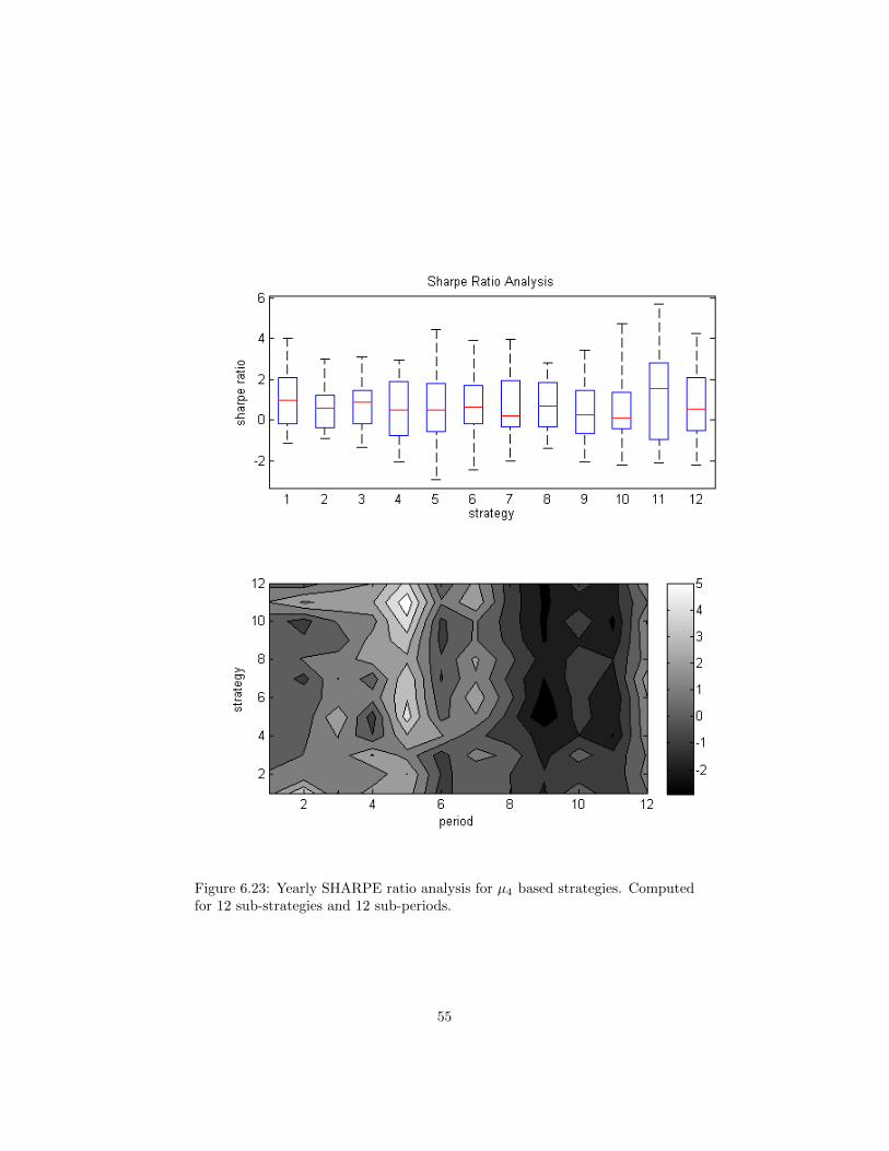
Figure 6.23: Yearly SHARPE ratio analysis for µ4 based strategies. Computedfor 12 sub-strategies and 12 sub-periods.

55

Figure 6.24: Yearly SHARPE ratio analysis for MAXIMUM DRAWDOWNof RETURNS based strategies. Computed for 12 sub-strategies and 12 sub-periods.

56

Figure 6.25: Yearly SHARPE ratio analysis for MAXIMUM DRAWDOWN ofVALUES based strategies. Computed for 12 sub-strategies and 12 sub-periods.

57

Figure 6.26: Yearly SHARPE ratio analysis for AVERAGE MAXIMUMDRAWDOWN of VALUES based strategies. Computed for 12 sub-strategiesand 12 sub-periods.

58

6.2.5 Transaction costs overview

Transaction costs are an important issue for investors. If a strategy is moreexpensive than it adds value, this strategy is useless. Here, transaction costs areevaluated in function of the total amount traded. At each end of sub-periods,portfolios are reconfigured, due to the investment strategy. These changes invalue are summed up to give the total amount traded, see figures 6.27, 6.28,6.29, 6.30, 6.31. Then transaction costs are a fraction of this amount. Notethat I choose to exclude the creation cost of the first portfolio correspondingto the cost of the first period. The total amount traded increases, if a strategyperforms well. Hence the cost of a good strategy is usually high. As shownin figures 6.27, 6.28, 6.29, this proposition is true with an exception: the 1stock strategy. This exception comes from the fact that the strategy one, selectthe same stock during consecutive periods. In this case, transaction costs areequal to zero. The most diversified is a portfolio, the less change in portfolioweights there is, hence the less costly is the strategy. Observe in figures quotedabove, that the equally weighted portfolio is the one, the most diversified andthe cheapest. In order to conclude, the table 6.4 gives an idea of the impactof transaction costs in strategies. In this example, transaction costs are equalto one percent of the total amount traded. It is for sure, excessive in the caseof hedge funds, but represents more or less the reality for individual investors.Comparing table 6.3 and 6.4, it is obvious, that the number of strategies under-performing the equally weighted portfolio, increases a lot if transaction costs arecounted. For strategies based on Maximum DrawDown of returns, it goes from0 to 1, for strategies based on Variance from 3 to 5 and for strategies based onµ4 from 3 to 8. It gives here a clear advantage for strategies based on MaximumDrawDown of returns.

59

Figure 6.27: Total transaction costs of the simulation for 4th MOMENT basedstrategies

Figure 6.28: Total transaction costs of the simulation for VARIANCE basedstrategies

60

Figure 6.29: Total transaction costs of the simulation for MAXIMUM DRAW-DOWN of RETURNS based strategies

Figure 6.30: Total transaction costs of the simulation for MAXIMUM DRAW-DOWN of VALUES based strategies

61

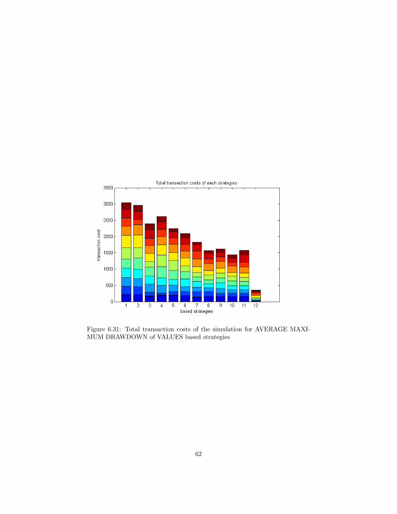
Figure 6.31: Total transaction costs of the simulation for AVERAGE MAXI-MUM DRAWDOWN of VALUES based strategies

62

Figure 6.32: How many times a strategy was the best of a period in the simu-lation for VARIANCE based strategies

6.2.6 Impact of the diversification - concrete cases

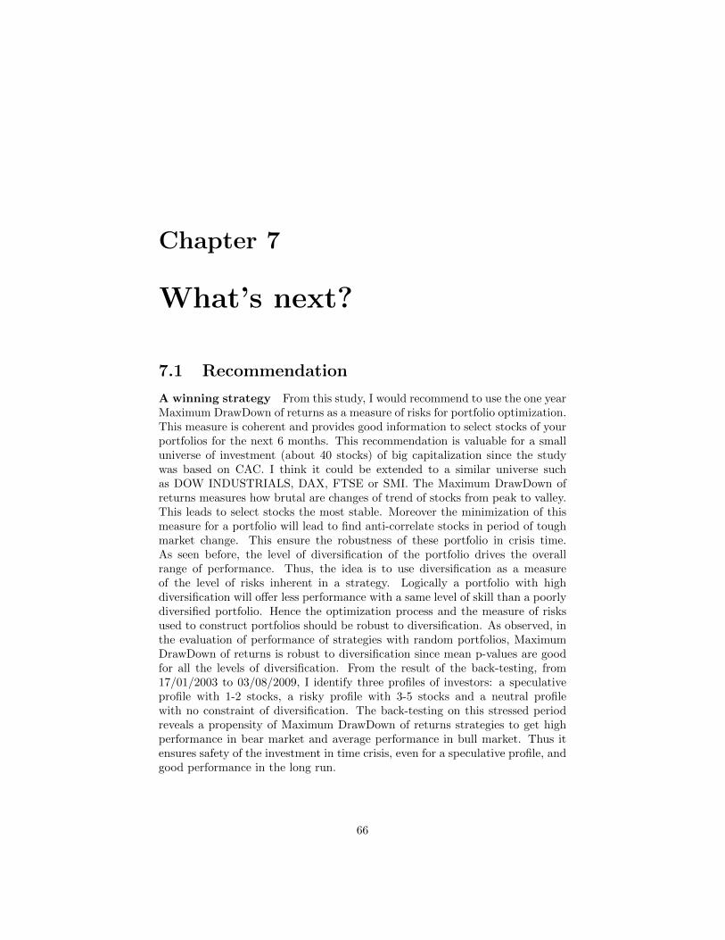
Diversification has a positive and a negative impact. The positive impactis the one that leads to lower risks by inhibition of unique risks in portfolio.The unique risk is a specific company risk. This company risk is diluted byother companies. Hence a diversified portfolio should only support market risks.The negative impact is the one that leads portfolio to loose opportunities ofgrowth. Imagine the case where few stocks are performing highly above themarket. For example, in the case of a universe containing 28 stocks and duringa period where only 2 stocks have positive performance, if a 10-stocks portfoliois created, it will at least contain 8 bad stocks. Figures 6.32, 6.33, 6.34, 6.35,6.36 represent the number of times, that a strategy earns the highest returnon a period. Results clearly show that exceptional performance comes frompoorly diversified portfolios. In conclusion, there is a trade-off to do betweenexceptional performance and low risks.

63

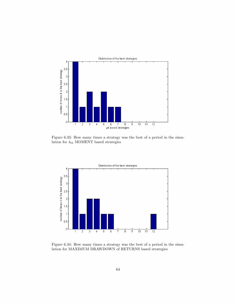
Figure 6.33: How many times a strategy was the best of a period in the simu-lation for 4th MOMENT based strategies

Figure 6.34: How many times a strategy was the best of a period in the simu-lation for MAXIMUM DRAWDOWN of RETURNS based strategies

64

Figure 6.35: How many times a strategy was the best of a period in the simu-lation for MAXIMUM DRAWDOWN of VALUES based strategies

Figure 6.36: How many times a strategy was the best of a period in the simu-lation for AVERAGE MAXIMUM DRAWDOWN of VALUES based strategies

65

Chapter 7

What’s next?

7.1 Recommendation

A winning strategy From this study, I would recommend to use the one yearMaximum DrawDown of returns as a measure of risks for portfolio optimization.This measure is coherent and provides good information to select stocks of yourportfolios for the next 6 months. This recommendation is valuable for a smalluniverse of investment (about 40 stocks) of big capitalization since the studywas based on CAC. I think it could be extended to a similar universe suchas DOW INDUSTRIALS, DAX, FTSE or SMI. The Maximum DrawDown ofreturns measures how brutal are changes of trend of stocks from peak to valley.This leads to select stocks the most stable. Moreover the minimization of thismeasure for a portfolio will lead to find anti-correlate stocks in period of toughmarket change. This ensure the robustness of these portfolio in crisis time.As seen before, the level of diversification of the portfolio drives the overallrange of performance. Thus, the idea is to use diversification as a measureof the level of risks inherent in a strategy. Logically a portfolio with highdiversification will offer less performance with a same level of skill than a poorlydiversified portfolio. Hence the optimization process and the measure of risksused to construct portfolios should be robust to diversification. As observed, inthe evaluation of performance of strategies with random portfolios, MaximumDrawDown of returns is robust to diversification since mean p-values are goodfor all the levels of diversification. From the result of the back-testing, from17/01/2003 to 03/08/2009, I identify three profiles of investors: a speculativeprofile with 1-2 stocks, a risky profile with 3-5 stocks and a neutral profilewith no constraint of diversification. The back-testing on this stressed periodreveals a propensity of Maximum DrawDown of returns strategies to get highperformance in bear market and average performance in bull market. Thus itensures safety of the investment in time crisis, even for a speculative profile, andgood performance in the long run.

66

A good back-testing A back-testing is relevant when applied to a periodlong enough to contain consecutive bull and bear markets. Indeed, it enablesinvestors to stress test their investment strategies. Moreover, the evaluation ofp-values, with random portfolios gives a really deep understanding of the perfor-mance of a strategy over time. It is important to understand the performanceof a strategy in detail to see if it provides value-added. From a study of ran-dom portfolios and after many comparisons, I suggest that the equally weightedportfolio, which represents the expected value of investors acting randomly, is areliable benchmark of performance. Actually, comparing the wealth producedby the equally weighted portfolio and a strategy is equivalent to compare thestrategy with a 50 percent p-value random portfolio.

7.2 To go further

Exploring all my ideas would have required more time. Some of them are listedbelow to go further in my study of investment strategy:

Impact of time This study have been done using one year of training dataand 6 months of holding in portfolio. Varying these durations may leadto other conclusions for the different indicators.

Impact of the universe The universe of study was quite small. What if itintegrates hundred of stocks of emerging markets?

Maximum DrawDown in multi-asset optimization What will be the re-sult of an optimisation of the Maximum DrawDowns of returns on a mixeduniverse of bonds and stocks.

Applying re-sampling for strategies based on moment of orders 2 and 4Re-sampling may lead to better results on this kind of measure based onreturns.

Combining market timing tool to asset allocation Some risk measures havebetter result in bear market, other in bull market. Predicting these mar-ket trends and adapting the optimized measure should produce exceptionalperformance.

Using hyper-spherical constraints in portfolio optimization and randomportfolios generation. It should significantly decrease the time of com-putation.

Short selling short selling is not studied in this study, because I don’t be-lieve that it is a position very useful for long run investment. However itcould be interesting to observe its effects on measures such as MaximumDrawDown.

67

List of Figures

2.1 Formulation of Mean-Variance optimization . . . . . . . . . . . . 62.2 Instability of the EFFICIENT FRONTIER moving at each peri-

ods. Efficient frontiers from 28 assets over 12 periods of 6 months. 62.3 DEVIATION of a portfolio from the EFFICIENT FRONTIER.

Same frontiers as figure 2.2 with the evolution of a portfolio takenon the first efficient frontier. A portfolio done in the Mean-Variance frameworks become rapidly inefficient. . . . . . . . . . . 7

2.4 SHRINKAGE Method - a trade off between sample covarianceand single index . . . . . . . . . . . . . . . . . . . . . . . . . . . 8

2.5 REVERSE ENGINEERING - Measure of distance from the sam-ple to the reverse engineering estimate. The factor alpha corre-sponds to the trade-off between the bias and the variance of ourestimation . . . . . . . . . . . . . . . . . . . . . . . . . . . . . . . 9

2.6 REVERSE ENGINEERING - Minimizing the distance of the re-verse engineering estimate to the sample estimate under the con-dition that the market efficient portfolio belows to the efficientfrontier . . . . . . . . . . . . . . . . . . . . . . . . . . . . . . . . 9

3.1 REPRODUCTION PROCESS using elite count, crossover andmutation. In this example the crossover rate is 0.8 and the elitecount is 2 . . . . . . . . . . . . . . . . . . . . . . . . . . . . . . . 15

3.2 A view of the scattered CROSSOVER function process. A ran-dom vector of bit is generated of the length equal the numberof assets in the portfolio. A zero means we select the weight ofparent 1 and a one the weight of parent 2 . . . . . . . . . . . . . 15

3.3 Gaussian MUTATION function adds a random number takenfrom a Gaussian distribution with mean 0 to each entry of theparent vector. . . . . . . . . . . . . . . . . . . . . . . . . . . . . . 16

4.1 Histogram of the 1000 RANDOM PORTFOLIOS generated withthe random and the normalize function. Returns are computedon a period of 6 months. The universe of study is composed on28 stocks of the CAC40 over 6 months. . . . . . . . . . . . . . . . 19

68

4.2 Graphics of RANDOM PORTFOLIOS sorted by increasing re-turns. The 1000 random portfolios were generated with the ran-dom and the normalize function. Returns are computed on aperiod of 6 months. The universe of study is composed on 28stocks of the CAC40 over 6 months.. . . . . . . . . . . . . . . . . 20

4.3 Histogram of the 1000 RANDOM PORTFOLIOS generated witha Genetic Algorithm at a Herfindahl Index of 1/3. Same periodand universe as figure 4.1. We can observe that the range ofreturns is much wider than this of figure 4.1 . . . . . . . . . . . . 21

4.4 Graphics of RANDOM PORTFOLIOS sorted by increasing re-turns. The 1000 random portfolios were generated with a Ge-netic Algorithm at a Herfindahl Index of 1/3. Same period anduniverse as figure 4.2. This graphics can be used to read the p-value of your strategy on this particular period and universe ifits herfindahl index is 1/3. . . . . . . . . . . . . . . . . . . . . . . 21

4.5 RANDOM PORTFOLIOS return for different level of the Herfind-ahl Index. Each line corresponds to a different p-value. The uni-verse of portfolios is composed of 28 stocks of the CAC40. Sixmonths of daily returns are used to evaluate portfolios returns.Thousand random portfolios were generated with a Genetic Al-gorithm for the 28 levels of the Herfindahl index ( 1,1/2,1/3...1/28) 22

5.1 Illustration of two MAXIMUM DRAWDOWNS . . . . . . . . . . 255.2 ENVELOP of returns taken by 1000 random portfolios calculated

for H0 = [1, 1/2 1/3, 1/4, 1/5, ..., 1/28] over a period of 121 days.H0 is the value of the Herfindahl Index the first day of the period. 27

5.3 VARIATION of the HERFINDAHL Index of a portfolio over aperiod of 122 days. H0 is equal to 0.1 The second graphic is azoom of the first one. We can observe that the variation of theHerfindahl Index are really small. Var(H) about equal to 10−7 . 28

6.1 Evolution of the CAC40. . . . . . . . . . . . . . . . . . . . . . . . 316.2 This table contains the different PERIODS OF DATA used dur-

ing the simulation. Training data are the data used to create aportfolio. Test data are the data used to evaluate the portfolio.Training data contained 260 days and test data 120 days. . . . . 32

6.3 END WEALTH of the different strategies at the date of 03/08/2009.Starting value of 100 the 19/01/2004. . . . . . . . . . . . . . . . 35

6.4 END WEALTH including TRANSACTION COSTS of 1 percentof the total value traded. Starting value of 100 the 19/01/2004. 35

6.5 Average RANDOM PORTFOLIOS P-VALUES of the differentstrategies for the period from 19/01/2004 to 03/08/2009. . . . . 35

6.6 Average yearly SHARPE RATIO of the different strategies forthe period from 19/01/2004 to 03/08/2009. . . . . . . . . . . . . 36

6.7 Result summary. Numbers represent the rank of strategies againsteach other. . . . . . . . . . . . . . . . . . . . . . . . . . . . . . . 36

69

6.8 Wealth evolution of VARIANCE based strategies from 19/01/2004to 03/08/2009. . . . . . . . . . . . . . . . . . . . . . . . . . . . . 39

6.9 Wealth evolution of 4th MOMENT based strategies from 19/01/2004to 03/08/2009. . . . . . . . . . . . . . . . . . . . . . . . . . . . . 39

6.10 Wealth evolution of MAXIMUM DRAWDOWN of RETURNSbased strategies from 19/01/2004 to 03/08/2009. . . . . . . . . . 40

6.11 Wealth evolution of MAXIMUM DRAWDOWN of VALUES basedstrategies from 19/01/2004 to 03/08/2009. . . . . . . . . . . . . . 40

6.12 Wealth evolution of Average MAXIMUM DRAWDOWN of VAL-UES based strategies from 19/01/2004 to 03/08/2009. . . . . . . 41

6.13 Comparison of the strategies in term of WEALTH at the end ofthe simulation from 19/01/2004 to 03/08/2009. All Herfindahlindex mixed. The red horizontal line represent the median. Theboundaries of the box represent the 25 and 75 quantile. Thewhiskers represent the minimum and maximum values. Maxi-mum values corresponds generally to high Hefindahl index (lookat the table 6.3 to see the corresponding values plotted here).This plot shows that strategies based on different measures ofrisks have different responses to diversification. . . . . . . . . . . 42

6.14 p-values analysis for 4th MOMENT based strategies. Resultscome from a random portfolios analysis with 1000 random portfo-lios of the same Herfindahl index as the analysed portfolio. Eachbox corresponds to the p-values of the 12 sub-periods for one levelof Herfindahl Index. In the box, the red horizontal line representthe median p-value over the 12 periods. The boundaries of thebox represent the 25 and 75 quantiles. The whiskers represent theminimum and maximum p-values. The map represents p-valuesfor a given sub-period and sub-strategies(the 12 sub-strategiescorrespond to the 12 different levels of Herfindahl index). . . . . 44

6.15 p-values analysis for VARIANCE based strategies. Results comefrom a random portfolios analysis with 1000 random portfolios ofthe same Herfindahl index as the analysed portfolio. Each boxcorresponds to the p-values of the 12 sub-periods for one level ofHerfindahl Index. In the box, the red horizontal line representthe median p-value over the 12 periods. The boundaries of thebox represent the 25 and 75 quantiles. The whiskers represent theminimum and maximum p-values. The map represents p-valuesfor a given sub-period and sub-strategies(the 12 sub-strategiescorrespond to the 12 different levels of Herfindahl index). . . . . 45

70

6.16 p-values analysis for MAXIMUM DRAWDOWN of RETURNSbased strategies. Results come from a random portfolios anal-ysis with 1000 random portfolios of the same Herfindahl indexas the analysed portfolio. Each box corresponds to the p-valuesof the 12 sub-periods for one level of Herfindahl Index. In thebox, the red horizontal line represent the median p-value overthe 12 periods. The boundaries of the box represent the 25 and75 quantiles. The whiskers represent the minimum and maximump-values. The map represents p-values for a given sub-period andsub-strategies(the 12 sub-strategies correspond to the 12 differentlevels of Herfindahl index). . . . . . . . . . . . . . . . . . . . . . 46

6.17 p-values analysis for MAXIMUM DRAWDOWN of VALUES basedstrategies. Results come from a random portfolios analysis with1000 random portfolios of the same Herfindahl index as the anal-ysed portfolio. Each box corresponds to the p-values of the 12sub-periods for one level of Herfindahl Index. In the box, thered horizontal line represent the median p-value over the 12 pe-riods. The boundaries of the box represent the 25 and 75 quan-tiles. The whiskers represent the minimum and maximum p-values. The map represents p-values for a given sub-period andsub-strategies(the 12 sub-strategies correspond to the 12 differentlevels of Herfindahl index). . . . . . . . . . . . . . . . . . . . . . 47

6.18 p-values analysis for AVERAGE MAXIMUM DRAWDOWN ofVALUES based strategies. Results come from a random portfo-lios analysis with 1000 random portfolios of the same Herfindahlindex as the analysed portfolio. Each box corresponds to thep-values of the 12 sub-periods for one level of Herfindahl Index.In the box, the red horizontal line represent the median p-valueover the 12 periods. The boundaries of the box represent the25 and 75 quantiles. The whiskers represent the minimum andmaximum p-values. The map represents p-values for a given sub-period and sub-strategies(the 12 sub-strategies correspond to the12 different levels of Herfindahl index). . . . . . . . . . . . . . . . 48

6.19 Return of strategies based on MAXIMUM DRAWDOWN of RE-TURNS, against random portfolios of p-value of 0.1 . In Period11, the market decreases and in period 12, it increases . . . . . . 50

6.20 Return of strategies based on 4thMOMENT, against random port-folios of p-value of 0.1 In Period 11, the market decreases and inperiod 12, it increases . . . . . . . . . . . . . . . . . . . . . . . . 51

6.21 Return of strategies based on VARIANCE, against random port-folios of p-value of 0.1 In Period 11, the market decreases and inperiod 12, it increases . . . . . . . . . . . . . . . . . . . . . . . . 52

6.22 Yearly SHARPE ratio analysis for VARIANCE based strategies.Computed for 12 sub-strategies and 12 sub-periods. . . . . . . . . 54

6.23 Yearly SHARPE ratio analysis for µ4 based strategies. Computedfor 12 sub-strategies and 12 sub-periods. . . . . . . . . . . . . . . 55

71

6.24 Yearly SHARPE ratio analysis for MAXIMUM DRAWDOWN ofRETURNS based strategies. Computed for 12 sub-strategies and12 sub-periods. . . . . . . . . . . . . . . . . . . . . . . . . . . . . 56

6.25 Yearly SHARPE ratio analysis for MAXIMUM DRAWDOWN ofVALUES based strategies. Computed for 12 sub-strategies and12 sub-periods. . . . . . . . . . . . . . . . . . . . . . . . . . . . . 57

6.26 Yearly SHARPE ratio analysis for AVERAGE MAXIMUM DRAW-DOWN of VALUES based strategies. Computed for 12 sub-strategies and 12 sub-periods. . . . . . . . . . . . . . . . . . . . . 58

6.27 Total transaction costs of the simulation for 4th MOMENT basedstrategies . . . . . . . . . . . . . . . . . . . . . . . . . . . . . . . 60

6.28 Total transaction costs of the simulation for VARIANCE basedstrategies . . . . . . . . . . . . . . . . . . . . . . . . . . . . . . . 60

6.29 Total transaction costs of the simulation for MAXIMUM DRAW-DOWN of RETURNS based strategies . . . . . . . . . . . . . . . 61

6.30 Total transaction costs of the simulation for MAXIMUM DRAW-DOWN of VALUES based strategies . . . . . . . . . . . . . . . . 61

6.31 Total transaction costs of the simulation for AVERAGE MAXI-MUM DRAWDOWN of VALUES based strategies . . . . . . . . 62

6.32 How many times a strategy was the best of a period in the sim-ulation for VARIANCE based strategies . . . . . . . . . . . . . . 63

6.33 How many times a strategy was the best of a period in the sim-ulation for 4th MOMENT based strategies . . . . . . . . . . . . . 64

6.34 How many times a strategy was the best of a period in the simula-tion for MAXIMUM DRAWDOWN of RETURNS based strategies 64

6.35 How many times a strategy was the best of a period in the simu-lation for MAXIMUM DRAWDOWN of VALUES based strategies 65

6.36 How many times a strategy was the best of a period in the sim-ulation for AVERAGE MAXIMUM DRAWDOWN of VALUESbased strategies . . . . . . . . . . . . . . . . . . . . . . . . . . . . 65

72

Bibliography

[1] Gilles Daniel, Didier Sornette and Peter Woehrmann, Look-Ahead Bench-mark Bias in Portfolio Performance Evaluation, Journal of Portfolio Man-agement 36 (1), 121-130 (Fall 2009).

[2] M.B. Abbes, Y. Boujelbene, and A. Bouri. Les profits des strategies mo-mentum: sous et/ou surreaction ou phenomene rationnel? cas du marchefrancais.

[3] P. ARTZNER, F. DELBAEN, J.M. EBER, and D. HEATH. COHERENTMEASURES OF RISK. Mathematical Finance, 9(3):203–228, 1999.

[4] G. Baquero, J. Horst, and M. Verbeek. Survival, look-ahead bias and theperformance of hedge funds. J. Fin. Quant. Anal., 40:493–504, 2005.

[5] J.P. Bouchaud and M. Potters. More stylized facts of financial markets:leverage effect and downside correlations. Physica A: Statistical Mechanicsand its Applications, 299(1-2):60–70, 2001.

[6] S.J. Brown, W.N. Goetzmann, and S.A. Ross. Survival. The Journal ofFinance, 50(3):853–873, 1995.

[7] P. Burns. Performance measurement via random portfolios. Newsletter.

[8] P. Burns and B. Statistics. Random Portfolios for Evaluating TradingStrategies. Burns, 2006.

[9] M.M. Carhart. On persistence in mutual fund performance. The Journalof Finance, 52(1):57–82, 1997.

[10] SC Chiam, KC Tan, and A.A. Mamun. A memetic model of evolutionaryPSO for computational finance applications. Expert Systems With Appli-cations, 36(2P2):3695–3711, 2009.

[11] E.F. Fama and K.R. French. Luck versus Skill in the Cross Section ofMutual Fund Alpha Estimates (http : //ssrn.com/abstract = 1356021).

[12] E.F. Fama and K.R. French. Common risk factors in the returns on stocksand bonds* 1. Journal of financial economics, 33(1):3–56, 1993.

73

[13] M. Grinblatt and S. Titman. The persistence of mutual fund performance.The Journal of Finance, 47(5):1977–1984, 1992.

[14] J. Liu, X. Jin, and K.C. Tsui. Autonomy oriented computing. KluwerAcademic.

[15] Y. Malevergne, P. Santa-Clara, and D. Sornette. Professor Zipfgoes to Wall Street (2009), NBER Working Paper No. 15295 (http ://ssrn.com/abstract = 1458280).

[16] H. Markowitz. Portfolio selection. The journal of finance, 7(1):77–91, 1952.

[17] R. Roll. A critique of the asset pricing theory’s tests Part I: On pastand potential testability of the theory* 1. Journal of financial economics,4(2):129–176, 1977.

[18] W.F. Sharpe. Capital asset prices: A theory of market equilibrium underconditions of risk. The Journal of Finance, 19(3):425–442, 1964.

74

Chapter 8

Annexes

8.1 Maximum DrawDown - Matlab Code

75

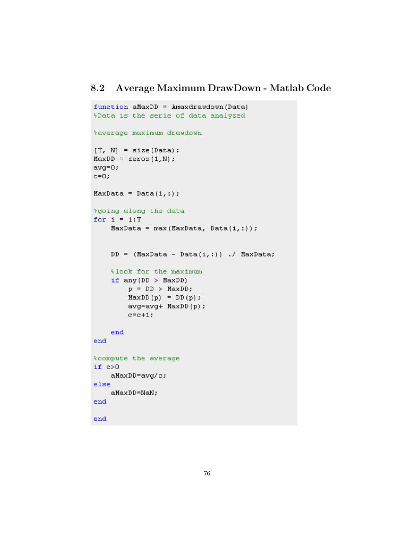
8.2 Average Maximum DrawDown - Matlab Code

76

Master Thesis -Software Documentation

Thibaut Simon

02/12/2009

Contents

1 Introduction 2

2 Optimization tool 32.1 How to use it? First use. . . . . . . . . . . . . . . . . . . . . . . . 32.2 Data . . . . . . . . . . . . . . . . . . . . . . . . . . . . . . . . . . 4

2.2.1 Input Data . . . . . . . . . . . . . . . . . . . . . . . . . . 42.2.2 Output Data . . . . . . . . . . . . . . . . . . . . . . . . . 4

2.3 Options . . . . . . . . . . . . . . . . . . . . . . . . . . . . . . . . 42.3.1 Genetic Algorithm Options . . . . . . . . . . . . . . . . . 42.3.2 Duration of training data and test data for the portfolio

construction . . . . . . . . . . . . . . . . . . . . . . . . . . 62.3.3 Fitness function for the portfolio construction . . . . . . . 6

3 Analysis tool 73.1 User Interface . . . . . . . . . . . . . . . . . . . . . . . . . . . . . 7

3.1.1 Aspect . . . . . . . . . . . . . . . . . . . . . . . . . . . . . 73.1.2 Possibilities . . . . . . . . . . . . . . . . . . . . . . . . . . 7

3.2 Data . . . . . . . . . . . . . . . . . . . . . . . . . . . . . . . . . . 83.2.1 Input Data . . . . . . . . . . . . . . . . . . . . . . . . . . 83.2.2 Output Data . . . . . . . . . . . . . . . . . . . . . . . . . 8

3.3 What do you want to analyse? . . . . . . . . . . . . . . . . . . . 8

4 To go further 104.1 What could be done to improve these tools? . . . . . . . . . . . . 104.2 Tips . . . . . . . . . . . . . . . . . . . . . . . . . . . . . . . . . . 104.3 FAQ . . . . . . . . . . . . . . . . . . . . . . . . . . . . . . . . . . 11

4.3.1 How to change fitness functions? . . . . . . . . . . . . . . 114.3.2 How to add a functionality to the analysis or optimization

tool? . . . . . . . . . . . . . . . . . . . . . . . . . . . . . . 11

5 Annexes 135.1 Optimization tool figures . . . . . . . . . . . . . . . . . . . . . . 145.2 Analysis tool figures . . . . . . . . . . . . . . . . . . . . . . . . . 21

1

Chapter 1

Introduction

This work is part of my thesis on ”Portfolio construction : How to achievebetter strategy through the use of Genetic Algorithm and non-linear objectivefunction based on new measures of risks and dependencies?”. During my studyof this subject I needed to solve optimization problem to construct portfolio andthen analyse their performance. That’s why I did two tools, with user-friendlyinterfaces, to help me in my work. These tools were at first really basic withoutuser-interface, but soon they became quite complex, due to the multiplicationof functions. Hence I decided to create a user interface that allows other peoplethan me, to use it easily in a future work. For this reason, I chose to do it inMATLAB. I will start with the optimization tool which makes the input dataused by the analysis tool. Then, I will explain how to use the analysis tool toexploit the result of the optimization tool. Finally, I will tale you what couldbe done to enhance the tool and how to do it.

2

Chapter 2

Optimization tool

The optimization tool allows to create portfolio from different objective func-tions. These objective functions correspond to allocation strategies. The opti-mization is done by a genetic algorithm coming from a library of Matlab. Youcan choose the precision of the genetic algorithm by setting up different options.You can as well choose the length of the data you use to create your portfolioand the duration you keep your portfolio before doing another one. The opti-miser use a file containing as data: the date of trading, the adjusted price of thestocks at the closure (see the section data below). This tool have the advantageto create portfolios from 12 different strategies over the length of data you want.Then you will be able to analyse these portfolio with the analysis tool.

The data I will use to present this tool are : 28 stocks coming from thefrench index CAC40 over about 1500 days from 2003.

2.1 How to use it? First use.

You will need to: first, launch Matlab, second, set the current directory tothe ”optimization directory”, then just write ”optimization” in the commandwindow (see figure 5.1). You can observe the window represented in figure 5.2.

If you want to create your first portfolio, just check the fitness you wantto use and click on the button ”launch computation”. The program will runthe optimization with the default value for the time-window and the geneticalgorithm. You can follow the evolution of the process in the command windowwhere you will see the period and the fitness currently being calculated. Resultof these optimizations are saved into the Matlab file ”portfolios.mat”. This fileis the file that will be required by the analysis tool. In order to understand howto choose the different parameters, I invite you to read the following parts.

3

2.2 Data

The aim of this section is to give you the ability to put the data you want intothe application. In order to be read by the program and produce the expectedresult, data should respect a format for the input data. The paragraph on theoutput data is done to understand what is stored in ”portfolios.mat” file.

2.2.1 Input Data

The input data come originally from .cls file found in yahoo finance (see figure5.5). This yahoo file contains a lot of field. For our purpose we need to keep onlythe adjusted close price and the date of each price (see figure 5.6). At the end allshould be gathered in a unique file that will be import into Matlab and saved as”data.mat”. The file ”data.mat” is a structure containing the numerical array”data” and the text array ”textdata”. These two array are necessary for thegood execution of the program. Figure 5.3 you can observe the numerical array”data” and figure 5.4 the text array ”textdata”. In this file, data should besorted from the most recent to oldest, like in the file provided by Yahoo finance.Each column corresponds to a stock. The first column correspond to the dateof each price in text.The two last columns contains the reference index (herethe CAC40) and the risk free rate (here the 13 weeks treasury bills). Look atthe screen-shots below to get a better view of these file and to understand theprocedure to follow in order to use your own data.

2.2.2 Output Data

The tool optimization produce the file ”portfolios.mat” which is a Matlabdata file containing the number of periods, the name of the fitness function, andthe portfolios structure. The portfolios structure store the portfolio weight, thetraining data of the period, the test data to evaluate the portfolio over the nextdays. And other data useful to analyse the portfolio as the reference index dataand risk free rate data over the period of test. You can see the details on thefigure 5.11. This file can be read next by the analysis tool to plot the interestingfigures and compare them.

2.3 Options

2.3.1 Genetic Algorithm Options

This program use the Genetic Algorithm of Matlab. In the interface youcan change three options that allow you to make more precise or quicker theoptimisation. Choices available here are the size of the population, the cross-over rate and the stall limit generation. However, it is possible to change otheroptions more fundamental by entering into the code of opt portfolio3.m andchanging gaoptimset settings. Look in the help of Matlab for more detailsabout the GA toolbox. Here is the list of options I used for the GA.

4

Population Options:

Population type , the individuals in the population are represented withthe data type double.

Population size specifies how many individuals there are in each gener-ation. With a large population size, the genetic algorithm searchesthe solution space more thoroughly, thereby reducing the chance thatthe algorithm will return a local minimum that is not a global min-imum. Here you can choose between 100 and 1000 with the sliderbutton.

Initial population specifies an initial population for the genetic algo-rithm. It is set as random.

Selection function: the Stochastic uniform selection function lays out a linein which each parent corresponds to a section of the line of length propor-tional to its scaled value. The algorithm moves along the line in steps ofequal size. At each step, the algorithm allocates a parent from the sectionit lands on. The first step is a uniform random number less than the stepsize.

Reproduction:

Crossover fraction specifies the fraction of the next generation, otherthan elite children, that are produced by crossover.

Elite count specifies the number of individuals that are guaranteed tosurvive to the next generation.

Mutation Options: the Gaussian mutation function adds a random numbertaken from a Gaussian distribution with mean 0 to each entry of the parentvector.

Crossover Options: The scattered crossover function creates a random binaryvector and selects the genes where the vector is a 1 from the first parent,and the genes where the vector is a 0 from the second parent, and combinesthe genes to form the child.

Stopping Criteria Options: The algorithm runs until the cumulative changein the fitness function value over Stall generations is less than or equal toFunction Tolerance. Here the number of generation is limited to 200 andstall limit generation can be chosen between 10 and 50 with the sliderbutton.

5

2.3.2 Duration of training data and test data for the port-folio construction

In order to study the influence of time, it is interesting to variate the amountof data you use to create your portfolio and the time you keep it. This is possibleto do with the two sliders button of the panel window parameters. If you increasethe holding duration of your portfolio, you decrease the final number of periods,hence you decrease the number of portfolios to calculate.

2.3.3 Fitness function for the portfolio construction

The fitness function can be choose by checking the name in the user interface.If you need to create or study new fitness function, you will have to enter alittle bit in the code. The fitness function is the mathematical expression ofyour strategy of risks mitigation. In order to implement your own innovativestrategy, you will need to create your own fitness function.The fitness function isthen used by the genetic algorithm to evaluate each portfolio. Fitness functionsare stored into the files fitness1.m, fitness2.m, ..., fitness12.m. Look at the lastchapter for more details.

6

Chapter 3

Analysis tool

The analysis tool has been developed to analyse portfolios coming from thetool optimization. It allow you to get a deep understanding of the performanceof each portfolio against the others. As you will see in this section, this interfaceallow you to analyse the portfolios under different perspectives.

3.1 User Interface

The analysis tool use a Matlab user interface that you can launch by enter-ing analyse ui in the command window, once you have set the correct currentdirectory.

3.1.1 Aspect

Figure 5.12, you can observe a screen-shot of the application. On the left,you choose what you want to observe and on the right, graphics are plotted.

3.1.2 Possibilities

Choices available for analysis are :

• Specific Fitness function

• Particular Period

• Global evolution of portfolios

• Which strategy for which period?

• What about transaction cost?

• Efficient frontier evolution

• Synthesis

7

A click on the button of your choice will plot the corresponding graphics intothe right panel. If you look on the bottom left panel,you will see a commandpanel where you can change parameters of the graphics and data plotted. Iadvise you to try the different possibilities which have all been selected for theirpertinence in portfolio analysis.

3.2 Data

3.2.1 Input Data

The tool optimization produce the file ”portfolios.mat” which is a Matlabdata file containing the number of periods, the name of the fitness function,and the portfolios structure. The portfolios structure store the portfolio weight,the training data of the period, the test data to evaluate the portfolio over thenext days. And other data useful to analyse the portfolio as the reference indexdata and risk free rate data over the period of test. You can see the details onthe figure 5.11. This file is the input data used by the analysis tool. Note thatfitness index and periods index in the portfolios structure should go from oneto n without discontinuities in order to works.

3.2.2 Output Data

No output data for the moment. Export to excel and image of graphics couldbe produce in further development.

3.3 What do you want to analyse?

Specific Fitness function Study a specific fitness function. A fitness functioncorrespond to an investment strategy. Each strategy lead to differentportfolio. You can choose witch function you want to analyse in the pop-up menu. Observe the evolution of the composition at each period. Lookat the evolution in value of the strategy. You can also look at the returnon each period to see when the portfolio perform the best.(see figure 5.12)

Particular Period Study all the different investment strategy for a selectedperiod. You can select the period you want to analyse in the pop-upmenu. For each period you will be able to compare the composition of theportfolios, the evolution of the value during the period and the returnsover the period.(see figure 5.13)

Global evolution of portfolios Plot the evolution of portfolios along all theperiods. Thus you can have a global view of the performance. The startingvalue of portfolios is 100.(see figure 5.14)

8

Which strategy for which period? You would like to know which strategyperform the best, or the most often. Trough the different plots, look atthe distribution of best strategies, or the repartition along periods of thebest strategy. Portfolios are ranked by rate of returns over the periods.Moreover you can check the composition of best portfolio to see if theyare diversified or not.(see figure 5.15)

What about transaction cost? It is interesting to have a look at the trans-action costs. They are calculated in absolute value. They correspond tothe change in value of each asset to get the new portfolio. Compare thecumulative costs of each strategy. Look which periods incur costs.(seefigure 5.16)

Efficient frontier evolution This section show the evolution of the efficientfrontier over time. It is done to show how big are the change of the markets.The efficient frontier is calculated from Markovitz portfolio theory withthe help of a quadratic solver. Often change are important and put somediscredit on the pertinence of the Markovitz theory.(see figure 5.17)

Synthesis Finally you need some figures to figure out how diversified is theportfolio with the Herfindahl index, what is the end value, the end valuetacking into account the transaction costs or the overall returns. Trans-action costs depend of who you are, hence you can choose the level oftransaction costs you want to apply in the pop-up menu.(see figure 5.18)

9

Chapter 4

To go further

This program has been developed in a limited amount of time. A lot canbe done to simplify its use. I will propose some idea of what can be done toimprove the utility and the easiness of use. This program has been done in theaim of constructing portfolios and analysing their performance and behaviourfor my master thesis. However I decided as it was really powerful for me, tomake it accessible and available for further use. It explains at some points, whyit is not always as functional as it should be or as I would like it to be.

4.1 What could be done to improve these tools?

Here are some idea to improve the functionality of this application. I will tryto give some hints to develop these ideas.

Compare strategy with different duration

Plot the evolution of the market index

Plot the Sharpe ratio

Export graphics to excel

Improve the process of data collection which is not automatic

Add a system to modify the fitness function easily

4.2 Tips

Tip 1: The user interface as been done using MATLAB GUIDE, which allowsto create nice interface. To launch this tool, write ”guide” in the commandwindow and load the optimization file ”optimization.fig”

10

Tip 2: The optimisation tool uses the Genetic Algorithm toolbox of Matlab.In order to get a wider view on the possibilities of GA in optimisation, youshould go looking in the help of the GA toolbox.

Tip 3: The analysis tool call 7 functions called analyse1.m, analyse2.m ....Each of these functions correspond to one choice of analysis user interface. Ifyou want to modify one of these functions, you will see, that they are built inthe same way. First, extract the interesting data from the structures portfolios.Second, make the calculation needed. Finally plot the interesting variables intothe interface with the use of handles.

4.3 FAQ

4.3.1 How to change fitness functions?

The fitness function is the mathematical expression of your strategy of risksmitigation. In order to implement your own innovative strategy, you will needto create your own fitness function.The fitness function is then used by thegenetic algorithm to evaluate each portfolio. Fitness functions are stored intothe files fitness1.m, fitness2.m, ..., fitness12.m. In order to create your ownfitness function, the easiest way, is to modify an existing one. Input variables offitness functions are the portfolio weights w and the data of returns returnsdata.You can basically evaluate what you want without worrying about linearityand so one. Each fitness function start by the command normalize(w) whichallows to keep the condition sum of weight equal to one. Then add z= .. whatyou want to minimize. Names of fitness functions are stored into the code fileoptimization.m in the variable fit name choice that you can change to put yourown name. See figure 4.1 for an example of fitness function.

4.3.2 How to add a functionality to the analysis or opti-mization tool?

These two applications can be modified. For example, it is possible to adda functionality to the Analysis tool. It will require to modify the interface fileanalysis-ui.fig and the m-file analysis-ui.m. In the interface file, you need forexample to add a button for your functionality. This new button will haveto be programmed in the m-file. A callback function is used to execute anaction following a click on the new button. I advice you to create a new m-fileanalysis8.m and to make your function of analysis inside, on the model of theother analysis1.m ... files. See tip 3 for more information.

11

Figure 4.1: Fitness function code in Matlab - minimization of the single actionmaxdrawdown for a specific level of the Herfindahl index

12

Chapter 5

Annexes

The figures referred before are grouped in this section. The optimization toolscreen-shots represent the process of importing new data for the tool. Figuresof the analysis section represent the different possibilities of analysis.

13

List of Figures

4.1 Fitness function code in Matlab - minimization of the single ac-tion maxdrawdown for a specific level of the Herfindahl index . . 12

5.1 Command window . . . . . . . . . . . . . . . . . . . . . . . . . . 155.2 Optimization interface . . . . . . . . . . . . . . . . . . . . . . . . 155.3 Numerical array ”data” in Matlab . . . . . . . . . . . . . . . . . 165.4 Text array ”textdata” in Matlab . . . . . . . . . . . . . . . . . . 165.5 Data file downloaded in yahoo finance . . . . . . . . . . . . . . . 175.6 Yahoo file treated by a VBA macro to keep only dates and prices 175.7 The file which should be imported to Matlab . . . . . . . . . . . 185.8 Import window 1 in Matlab . . . . . . . . . . . . . . . . . . . . . 185.9 Import window 2 in Matlab . . . . . . . . . . . . . . . . . . . . . 195.10 Save window in matlab to produce ”data.mat” which is needed

by the program . . . . . . . . . . . . . . . . . . . . . . . . . . . . 195.11 Details of data contained in the portfolios structure . . . . . . . . 205.12 Study of a specific fitness function . . . . . . . . . . . . . . . . . 215.13 Comparison of the different strategies for a specific period . . . . 215.14 Overview of the evolution of the strategies . . . . . . . . . . . . . 225.15 Which strategy perform the best? . . . . . . . . . . . . . . . . . . 225.16 Study of the transaction cost . . . . . . . . . . . . . . . . . . . . 235.17 Plot the evolution of efficient frontier . . . . . . . . . . . . . . . . 235.18 Synthesis of the performance of the different strategies . . . . . . 24

5.1 Optimization tool figures

14

Figure 5.1: Command window

Figure 5.2: Optimization interface

15

Figure 5.3: Numerical array ”data” in Matlab

Figure 5.4: Text array ”textdata” in Matlab

16

Figure 5.5: Data file downloaded in yahoo finance

Figure 5.6: Yahoo file treated by a VBA macro to keep only dates and prices

17

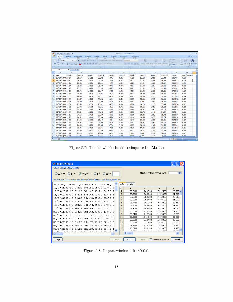
Figure 5.7: The file which should be imported to Matlab

Figure 5.8: Import window 1 in Matlab

18

Figure 5.9: Import window 2 in Matlab

Figure 5.10: Save window in matlab to produce ”data.mat” which is needed bythe program

19

Figure 5.11: Details of data contained in the portfolios structure

20

5.2 Analysis tool figures

Figure 5.12: Study of a specific fitness function

Figure 5.13: Comparison of the different strategies for a specific period

21

Figure 5.14: Overview of the evolution of the strategies

Figure 5.15: Which strategy perform the best?

22

Figure 5.16: Study of the transaction cost

Figure 5.17: Plot the evolution of efficient frontier

23

Figure 5.18: Synthesis of the performance of the different strategies

24