University of New England

School of Economics

AN EMPIRICAL ANALYSIS OF THE PROPOSED AUSTRALIA-JAPAN FREE TRADE AGREEMENT

by

MAHINDA SIRIWARDANA AND BRIAN DOLLERY

No. 2003-2

Working Paper Series in Economics

ISSN 1442 2980

http://www.une.edu.au/febl/EconStud/wps.htm

Copyright © 2003 by Mahinda Siriwardana and Brian Dollery. All rights reserved. Readers may make verbatim copies of this document for non-commercial purposes by any means, provided this copyright notice appears on all such copies. ISBN 1 86389 829 8

2

AN EMPIRICAL ANALYSIS OF THE PROPOSED AUSTRALIA-JAPAN

FREE TRADE AGREEMENT

MAHINDA SIRIWARDANA AND BRIAN DOLLERY∗∗

Abstract

The success of the proposed Australia-Japan Free Trade Agreement will depend to a

considerable degree on the manner in which it deals with the problem of agricultural

trade between the two countries. This paper seeks to provide a quantitative

assessment of the potential impact of an Agreement under two scenarios: full

agricultural trade and no agricultural trade. We undertake simulations using the

Global Trade Analysis Project (GTAP) model to estimate the effects of liberalized

trade between Australia and Japan. Our results provide some preliminary indication

of the magnitude of the welfare gains involved under the two trade regimes

envisaged.

Key Words: Australia-Japan Free Trade Agreement; Computable general equilibrium

∗∗ Mahinda Siriwardana is an Associate Professor in the School of Economics at the University of New England, and Brian Dollery is a Professor in the School of Economics at the University of New England. Contact information: School of Economics, University of New England, Armidale, NSW 2351, Australia. Email: bdollery@metz.une.edu.au.

3

An Empirical Analysis of the Proposed Australia-Japan Free Trade

Agreement 1. Introduction

During his official state visit to Canberra on 9 May 2002, Prime Minister Junichiro

Koizumi of Japan formally announced that Japan sought a Free Trade Agreement (FTA) with

Australia and was willing to negotiate towards that end. Australian Prime Minister John

Howard responded positively to this proposal. It would thus appear that a protracted period of

negotiations between the two countries will now begin in order to draft a mutually

satisfactory bilateral FTA. An FTA between Australia and Japan would represent part of the

broader “hub-and-spokes” Growing East Asia Community strategy developed by Japan, and

in this sense would augment the existing Japan-Singapore FTA. Under this strategy, Japan

would cement its role as the dominant economy at the centre of Asia and strengthen its ties

with surrounding nations in the Asia-Pacific region.

A critical feature of the Japan-Singapore FTA resides in the fact that the potential for

agricultural imports from Singapore into Japan is minimal (Scollay, 2001). Indeed, various

statements by senior Japanese foreign trade officials indicate that that the Japan-Singapore

FTA represents a case of “learning-by-doing” in bilateral trade negotiations with Asian

countries, with Singapore acting as a “training ground” for further preferential trading

agreements, such as the proposed Australia-Japan FTA (Scollay, 2001).

The question of agricultural trade between Australia and Japan is bound to raise many

difficulties, especially the problem of Australian access to the Japanese domestic market.

However, with the ongoing economic stagnation of the Japanese economy, and the impetus

this provides for economic reform in Japan, it surely cannot be ruled out.

Given the potential significance of the Australia-Japan FTA, this paper offers some

preliminary findings on its impact on both the economies of Japan and Australia. We use a

4

computable general equilibrium (CGE) model developed at the Global Trade Analysis

Project (GTAP) to examine the effects of trade liberalization envisaged by the proposed FTA.

The paper itself comprises six main sections. Section 2 provides a brief synopsis of

the literature on trade liberalization and the light it sheds on a likely Australia-Japan FTA.

Section 3 outlines the economic structure of relevant region and contrasts it with the broader

global economy. Section 4 reviews the GTAP model employed for the trade simulations.

Section 5 examines two trade liberalization scenarios used in the GTAP simulations; an FTA

excluding agriculture and an FTA including agriculture. Section 6 analyses the results of the

simulation exercises. The paper ends with some brief concluding comments in section 7.

2. Trade Liberalization and Bilateral Free Trade Agreements

After Jacob Viner’s (1950) seminal demonstration that preferential trading

arrangements may induce net welfare losses if the effects of trade diversion overwhelm those

of trade creation, economists have long been sceptical of bilateral foreign trade treaties. A

voluminous literature now exists on the theoretical analysis of FTAs (see, for instance,

Bhagwati and Panagariya (1996)). Much less work has been done on the empirical analysis of

FTAs, especially on the “dynamics of how these agreements have been negotiated and

implemented, their impact on the pattern of trade and investment flows, their positive or

negative externalities with respect to the multilateral system, their effects on the productive

and investment decisions in each of the parties involved, and more generally issues regarding

the political process behind the negotiating process” (Estevadeordal, 2000, p.141).

Nevertheless, a substantial empirical literature has been developed using CGE

analysis, including work on Asia-Pacific Economic Cooperation (APEC) trade liberalization

initiatives and its sectoral manifestations, such as the Early Voluntary Sector Liberalization

(EVSL). This empirical literature has been comprehensively surveyed by both Petri (1997)

5

and Scollay and Gilbert (2000). In general, it appears that whatever form trade liberalization

takes, it generates welfare gains, most of which stem from agriculture.

A bilateral preferential trade agreement along the lines of the proposed Australia-

Japan FTA represents a legally binding agreement with the objective of bringing about closer

economic integration between two countries. In terms of such an agreement, the two

countries concerned undertake to provide each other with preferential access to their domestic

markets for goods and services. Favourable treatment of this kind typically embraces the

removal (or at least reduction) of import tariffs, the relaxation of quantitative import

restrictions, and a more relaxed application of existing domestic regulations. FTAs typically

also contain provisions for enhancing investment in the countries concerned and may often

stress technological relationships. Agreements generally hinge on voluntarism and are “open-

ended” in the sense that the ongoing nature of discussions about further trade liberalization is

emphasized.

The proposed Australia-Japan FTA should be viewed in the context of recent

developments in international trade in the Asia-Pacific region. Both APEC’s meeting in

September 1999 and the subsequent World Trade Organization’s (WTO) Seattle ministerial

in December 1999 struggled to find meaningful consensus amongst member countries. One

consequence of faltering multilateralism has been the sharp upsurge of interest in preferential

bilateral trade agreements. Scollay (2001, p.1145) has identified no less than 20 proposals for

new preferential trading agreements among APEC members at various stages of negotiation.

An Australia-Japan FTA would thus be a further addition to this mushrooming genre.

3. Economic Structure and Trade Pattern

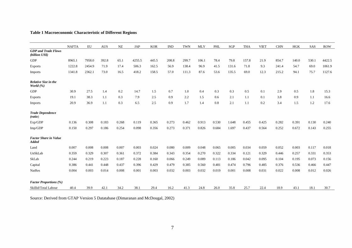
Table 1 presents data on GDP, external trade, trade dependence, factor endowments,

and the relative size of the economic regions included in the model. The data are remarkably

6

asymmetrical among regions with respect to their relative sizes of GDP, exports and imports.

The economic prominence of high-income entities (NAFTA, EU, and JAP) is evident. These

three regions together account for about 73 per cent of world GDP, 65 per cent of exports and

64 per cent imports. Compared to Japan, Australia’s comparative size in the global economy

is relatively small and one would thus expect this to carry weight in bilateral trade

negotiations. Nevertheless, the trade dependence ratios reveal that Australia is a more open

economy than Japan.

7

Table 1 Macroeconomic Characteristic of Different Regions

NAFTA EU AUS NZ JAP KOR IND TWN MLY PHL SGP THA VIET CHN HGK SAS ROW GDP and Trade Flows (billion US$)

GDP 8965.1 7958.0 392.8 65.1 4255.5 445.5 208.8 299.7 106.1 78.4 79.8 157.8 21.9 854.7 140.0 530.1 4422.5

Exports 1222.8 2454.9 71.9 17.4 506.3 162.5 56.9 138.4 96.9 41.5 131.6 71.8 9.3 241.4 54.7 69.0 1061.9

Imports 1341.8 2362.1 73.0 16.5 418.2 158.5 57.0 111.3 87.6 53.6 135.5 69.0 12.3 215.2 94.1 75.7 1127.6

Relative Size in the World (%)

GDP 30.9 27.5 1.4 0.2 14.7 1.5 0.7 1.0 0.4 0.3 0.3 0.5 0.1 2.9 0.5 1.8 15.3

Exports 19.1 38.3 1.1 0.3 7.9 2.5 0.9 2.2 1.5 0.6 2.1 1.1 0.1 3.8 0.9 1.1 16.6

Imports 20.9 36.9 1.1 0.3 6.5 2.5 0.9 1.7 1.4 0.8 2.1 1.1 0.2 3.4 1.5 1.2 17.6

Trade Dependence (ratio)

Exp/GDP 0.136 0.308 0.183 0.268 0.119 0.365 0.273 0.462 0.913 0.530 1.648 0.455 0.425 0.282 0.391 0.130 0.240

Imp/GDP 0.150 0.297 0.186 0.254 0.098 0.356 0.273 0.371 0.826 0.684 1.697 0.437 0.564 0.252 0.672 0.143 0.255

Factor Share in Value Added

Land 0.007 0.008 0.008 0.007 0.003 0.024 0.080 0.009 0.048 0.065 0.005 0.034 0.059 0.052 0.003 0.117 0.018

UnSkLab 0.359 0.329 0.307 0.361 0.372 0.384 0.343 0.354 0.270 0.322 0.334 0.121 0.329 0.446 0.257 0.331 0.353

SkLab 0.244 0.219 0.223 0.187 0.228 0.160 0.066 0.249 0.089 0.113 0.186 0.042 0.095 0.104 0.195 0.073 0.156

Capital 0.386 0.441 0.448 0.437 0.396 0.429 0.479 0.385 0.560 0.481 0.474 0.796 0.485 0.376 0.536 0.466 0.447

NatRes 0.004 0.003 0.014 0.008 0.001 0.003 0.032 0.003 0.032 0.019 0.001 0.008 0.031 0.022 0.008 0.012 0.026

Factor Proportions (%)

Skillid/Total Labour 40.4 39.9 42.1 34.2 38.1 29.4 16.2 41.3 24.8 26.0 35.8 25.7 22.4 18.9 43.1 18.1 30.7

Source: Derived from GTAP Version 5 Datatabase (Dimaranan and McDougal, 2002)

8

Data reported in Table 1 also point to the significance variation in factor endowments

amongst regions. For example, the high-income regions are relatively abundant in skilled

labour and capital in comparison to developing regions. It is also noticeable that developing

regions are endowed with higher shares of unskilled labour. Australia and Japan show

remarkably similar shares in unskilled labour, skilled labour and capital, although Australia is

relatively better endowed with land and natural resources. Moreover, Australia has more

skilled labour in the labour force (or 42 per cent) in comparison to Japan (at 29 per cent).

Figure 1: Australia's Trade with Japan, 1985-2000

0

2000

4000

6000

8000

10000

12000

14000

1985

1986

1987

1988

1989

1990

1991

1992

1993

1994

1995

1996

1997

1998

1999

2000

Year

US

$mill

ion

Exports Imports TBSource: Based on data from IMF, Direction of Trade Statistics Yearbook (various issues)

Figure 1 depicts Australia’s trade with Japan from 1985 to 2000. Over this 16-year period,

trade between Australia and Japan has shown substantial growth. Furthermore, Australian

exports exceed imports throughout the period showing a significant trade surplus with Japan.

9

4. Characteristics of the GTAP Model

The analytical framework used to quantify the impact of bilateral tariff reductions is

the well-known GTAP model (Hertel, 1996). It is a comparative-static, multi-regional CGE

model of the Johansen type comprising a system of linear equations in percentage change of

variables. The modelling of each region in GTAP is based on the ORANI model (Dixon et

al., 1982). In this paper, we employed the latest version of the GTAP model, together with

version four of the database that employs 45 regions and 50 sectors in each region.

The GTAP model has a number of notable features which include product

differentiation by country of origin, explicit recognition of savings by regional economies, a

capital goods producing sector in each region to service investment, international mobility of

capital, multiple trading regions, multiple goods and primary factors, empirically-based

differences in production technology and consumer preferences across regions, and explicit

recognition of a world transport sector. It also accommodates several policy variables,

including taxes and subsidies on commodities and primary factors. This makes the model

extremely attractive to policy economists.

In each region both factor and commodity markets are assumed to be perfectly

competitive. Producers operate under constant returns to scale (CES), where the technology is

described by the Leontief and CES functions. Two broad categories of inputs into production

are identified; intermediate inputs and primary factors. Each regional sector is designated as

choosing a mixture of inputs to minimise total cost for a given level of output. At the first

level, producers use composite units of intermediate inputs and primary factors in fixed

proportions according to a Leontief function. At the second level of the production nest,

intermediate input composites are obtained as combinations of imported bundles and

domestic goods of the same input-output class, and primary factor input composites are

created as combinations of skilled labour, unskilled labour, capital, land, and natural

10

resources. A CES function is used in forming both types of composites. Finally, at the third

level, imported bundles are created via a CES aggregation of imported goods of the same

class from each region.

On the demand side, the GTAP model adopts a sophisticated specification of

consumer behaviour that allows for differences in both price and income responsiveness of

demand in different regions, depending on the level of development and regional specific

demand patterns. Each region has a single representative household that receives all the

income generated through payments to primary factors and net tax revenue. The

representative household is governed by an aggregate utility function over private household

consumption, government consumption and savings. The aggregate utility is modelled using

a Cobb-Douglas function with constant expenditure shares. Government consumption is also

described by a Cobb-Douglas function over composite commodities where the demand for

the latter is a CES aggregation of imports and domestic goods. Private household

consumption is explained by a CDE (Constant Difference of Elasticities) expenditure

function. Households purchase bundles of commodities where the bundles are a CES

aggregation of domestic goods and imported bundles. The imported bundles are then formed

by a CES aggregation of imports from different regions.

Capital accumulation occurs in each region according to a technology that is similar

to producing current goods, except that it requires only domestic and imported intermediate

inputs. This capital creation services the investment that is financed by a global pool of

savings. Each region contributes a share of its income to a savings pool at a global bank that

is designed to mediate world savings and investment. Two methods are available in the

standard GTAP model for allocating global savings to investment in each region. In the first

place, global savings are allocated across investment in a fixed proportion to the total savings,

such that the regional composition of global investment remains unaltered. The second

11

method allows investment to take place in each region according to the prevalent relative

rates of return.

Version five of the GTAP database is used in the following empirical analysis. This

version divides the world into 66 regions and each region contains 57 sectors (or

commodities). Given the focus of this study, we aggregate the database into 17 regions and

20 sectors as shown in Appendix Table A1. Since our focus falls exclusively on the proposed

bilateral FTA between Australia and Japan, the regional aggregation highlights the

importance of other trading partners to the proposed FTA. The sectoral aggregation

framework was designed to distinguish agricultural commodities (or sectors) that are

important for the present analysis.

5. Trade Policy Scenarios

If a FTA is formed between Australia and Japan, then a number of changes are

projected to occur in bilateral tariffs. Australia is expected to abolish all the tariff barriers (as

shown in Table 2) on imports from Japan and Japan will do the same on imports from

Australia. Tariffs imposed on imports sourced from other trading partners to Australia and

Japan are assumed to remain unchanged. With the elimination of tariffs on bilateral basis,

both the prices of Japanese goods sold in Australia and Australian products sold in Japan will

fall by the amount of these import duties.

To capture the effects of Australia-Japan FTA, two simulation experiments were

carried out using GTAP model and its database aggregation, as we have already discussed.

The two liberalisation scenarios considered below reflect two broad options available to the

proposed Australia-Japan FTA.

(i) Scenario 1: All bilateral tariffs are removed between Australia and Japan and the

benefits of such liberalization are confined to the FTA. This necessarily implies

12

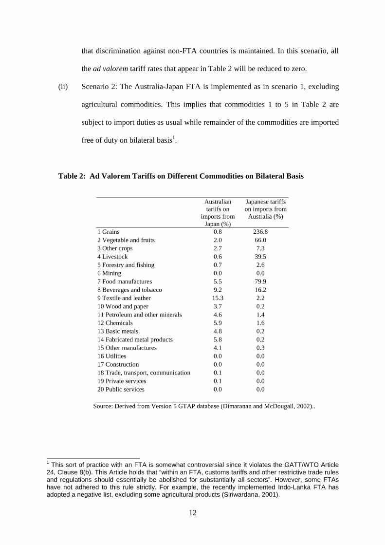
that discrimination against non-FTA countries is maintained. In this scenario, all

the ad valorem tariff rates that appear in Table 2 will be reduced to zero.

(ii) Scenario 2: The Australia-Japan FTA is implemented as in scenario 1, excluding

agricultural commodities. This implies that commodities 1 to 5 in Table 2 are

subject to import duties as usual while remainder of the commodities are imported

free of duty on bilateral basis1.

Table 2: Ad Valorem Tariffs on Different Commodities on Bilateral Basis

Australian

tariifs on imports from

Japan (%)

Japanese tariffs on imports from

Australia (%)

1 Grains 0.8 236.8 2 Vegetable and fruits 2.0 66.0 3 Other crops 2.7 7.3 4 Livestock 0.6 39.5 5 Forestry and fishing 0.7 2.6 6 Mining 0.0 0.0 7 Food manufactures 5.5 79.9 8 Beverages and tobacco 9.2 16.2 9 Textile and leather 15.3 2.2 10 Wood and paper 3.7 0.2 11 Petroleum and other minerals 4.6 1.4 12 Chemicals 5.9 1.6 13 Basic metals 4.8 0.2 14 Fabricated metal products 5.8 0.2 15 Other manufactures 4.1 0.3 16 Utilities 0.0 0.0 17 Construction 0.0 0.0 18 Trade, transport, communication 0.1 0.0 19 Private services 0.1 0.0 20 Public services 0.0 0.0

Source: Derived from Version 5 GTAP database (Dimaranan and McDougall, 2002)..

1 This sort of practice with an FTA is somewhat controversial since it violates the GATT/WTO Article 24, Clause 8(b). This Article holds that “within an FTA, customs tariffs and other restrictive trade rules and regulations should essentially be abolished for substantially all sectors”. However, some FTAs have not adhered to this rule strictly. For example, the recently implemented Indo-Lanka FTA has adopted a negative list, excluding some agricultural products (Siriwardana, 2001).

13

The GTAP model allows for different scenarios concerning factor markets and

macroeconomic closure. The tariff simulations using the GTAP model reported in this paper

were conducted within a long-run framework. Rates of return are equalised across regions,

with capital mobility taking place across regions. Investment occurs in each region during the

period of tariff reduction thus ensuring that sum of the regional investment matches with the

changes in the global savings. Unlike in the standard long-run closure of GTAP, wage rates

are fixed exogenously and the supply of labour is endogenised. The theoretical rationale for

this is that unemployed labour can be drawn on by industries in the event of increased

production with trade liberalisation.

6. Simulation Results

The trade policy scenarios examined in this paper deal with full liberalization of

Australia-Japan trade and partial liberalisation where trade in agricultural goods between

Australian and Japan are subject to import duties at the existing rates. On the basis of GTAP

model simulations, this section reports the results that provide the estimated effects of the

bilateral trade liberalisation on important macroeconomic variables, industry outputs, and

economic welfare. In order to distinguish the outcomes of exclusion of agricultural trade from

proposed FTA, the results are presented under the two different scenarios outlined earlier. In

particular, it is important to determine whether high Japanese tariff barriers on agricultural

imports under option (ii) make economic sense when it comes to negotiating an FTA with

Australia. From the perspective of Japanese trade negotiators, these findings will have

momentous policy implications.

14

Full Trade Liberalisation Scenario

The macroeconomic effects of an Australia-Japan FTA in its full liberalization form

are shown in columns (1)–(6) in Table 3. Several important points emerge from these

projections. The removal of tariffs between Japan and Australia leads to a substantial increase

(14 per cent) in real GDP of Australia. Whereas Australia appears to be the outright gainer in

terms of GDP, Japan emerges as a marginal looser (0.58 per cent) from the FTA. Except for

New Zealand, all other non-member regions experience a small fall in their real GDP as a

result of the Australia-Japan FTA. Since non-members are discriminated against under the

proposed FTA, trade diversion has a negative impact on their economies.

The tariff policy reforms under the proposed FTA bring about substantial changes in

trade performance in Australia compared to Japan. Australian exports are projected to grow

by 12 per cent and imports to increase by about 17 per cent. This will still leave a trade

surplus for Australia that is estimated to be around US$ 735.5 million. Australia observes a 5

per cent improvement in terms trade: this explains its remarkable increase in real GDP as a

result of the full implementation of the FTA. By contrast, Japan is projected to experience a

trade deficit (around US$ 2536.3 million) and its exports and imports are expected to increase

by 0.9 per cent and 1.1 per cent respectively. Unlike Australia, the terms of trade for Japan

deteriorate by about 0.5: this is probably responsible for the small loss in real GDP.

15

Table 3: Macroeconomic and Trade Performance Results of Australia-Japan FTA

Full Trade Liberalisation Scenario Trade Liberalisation Excluding Agriculture Scenario

Real GDP

Terms of Trade

Export Volume

Import Volume

Trade Balance

(US$ million)

Equivalent Variation (EV) (US$ million)

Real GDP

Terms of Trade

Export Volume

Import Volume

Trade Balance

(US$ million)

Equivalent Variation (EV) (US$ million)

(1) (2) (3) (4) (5) (6) (7) (8) (9) (10) (11) (12) NAFTA -0.28 -0.04 -0.25 -0.32 735.28 -23185.5 -0.21 -0.01 -0.18 -0.22 673.9 -17132.5 EU -0.11 0.00 -0.09 -0.12 605.5 -7652.6 -0.10 0.00 -0.09 -0.11 463.63 -7254.4 AUS 14.42 5.14 12.34 16.83 735.52 54803.6 12.33 1.83 12.36 13.99 149.97 44670.6 NZ 0.78 -0.05 0.64 0.48 26.45 447.4 0.34 -0.02 0.33 0.25 14.69 194.3 JAP -0.58 -0.57 0.95 1.16 -2536.34 -23205.2 -0.40 -0.15 0.81 1.19 -1519.06 -15332.0 KOR -0.23 -0.03 -0.29 -0.33 -3.14 -949.8 -0.25 -0.02 -0.28 -0.29 -26.44 -1006.7 IND -0.27 -0.24 -0.53 -0.84 43.71 -641.0 -0.22 -0.11 -0.37 -0.50 9.63 -474.4 TWN -0.35 -0.03 -0.35 -0.37 -100.59 -1009.6 -0.32 -0.03 -0.32 -0.34 -92.52 -923.9 MLY -0.19 -0.02 -0.30 -0.35 7.34 -201.8 -0.11 -0.02 -0.17 -0.20 -5.52 -121.7 PHL -0.21 -0.07 -0.32 -0.37 32.89 -185.4 -0.20 -0.04 -0.25 -0.29 29.02 -158.1 SGP -0.13 -0.02 -0.12 -0.14 6.86 -114.8 -0.09 -0.01 -0.10 -0.10 6.32 -74.8 THA -0.44 -0.11 -0.50 -0.58 -39.73 -684.8 -0.41 -0.12 -0.46 -0.52 -53.64 -650.3 VIET -0.37 -0.02 -0.47 -0.49 13.75 -74.3 -0.47 -0.07 -0.51 -0.56 14.82 -97.5 CHN -0.20 -0.08 -0.31 -0.37 -108.36 -1712.0 -0.17 -0.05 -0.25 -0.28 -132.21 -1418.1 HGK -0.16 -0.01 -0.14 -0.18 77.59 -212.8 -0.15 -0.01 -0.14 -0.16 70.98 -198.9 SAS -0.14 -0.22 -0.45 -0.72 63.49 -831.6 -0.14 -0.11 -0.29 -0.41 28.47 -731.6 ROW -0.15 -0.02 -0.13 -0.18 439.77 -5951.4 -0.13 -0.01 -0.12 -0.16 367.98 -5139.2

16

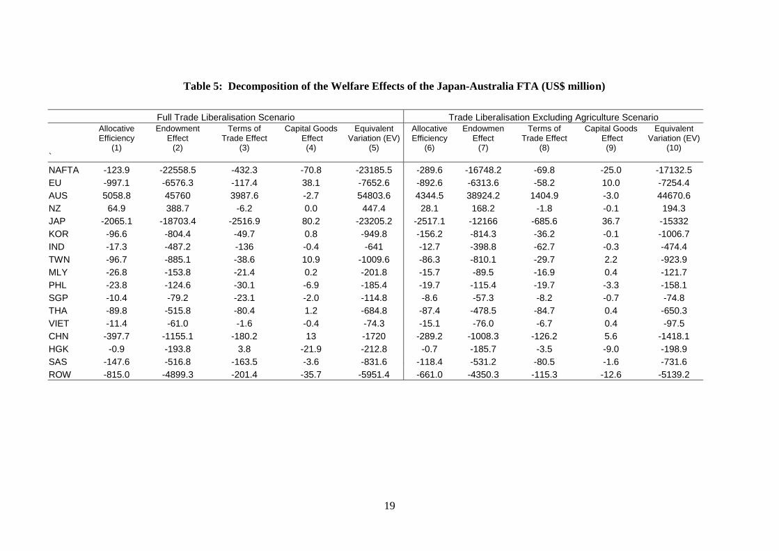
We now turn to the estimated welfare changes from the GTAP simulations. Column

(6) in Table 3 outlines the equivalent variation (EV) in dollar terms. The EV is an absolute

monetary measure of welfare improvement in terms of income that results from the fall in

import prices when tariffs are reduced or eliminated. The estimated EV seems to follow the

same pattern as changes in real GDP for Australia and Japan. As shown in Table 3, Australia

is expected to have a significant welfare gain due to the FTA whereas Japan is likely to face a

considerable loss in welfare. The welfare decomposition reported in Table 5 highlights the

causes of welfare changes in response to tariff elimination under the FTA. Australia’s gain in

welfare is largely due to the endowment effect and the improvement in allocative efficiency

followed by the terms of trade effect. The endowment effect dominates the welfare outcome

for Australia accounting for the employment gain (see Table 4) resulting from trade

liberalization. The negative impact on the welfare of the Japanese economy largely stems

from the endowment effect. Unlike in Australia, there is a positive capital goods effect in

Japan. This is similar to the terms of trade effect: it measures the price of purchasing capital

goods at home relative to the price of savings in the world market. It is also important to note

the significant influence of the allocative efficiency and terms of trade effects in reducing

welfare in Japan.

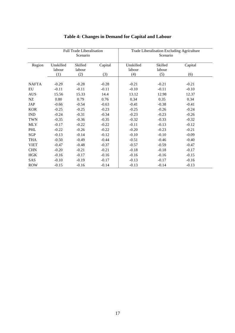
The results reported in Table 4 (columns 2-4) may be seen as factor market

adjustments in response to bilateral tariff elimination. From Australia’s perspective, with free

trade under the FTA, demand for both skilled and unskilled labour and capital will increase in

line with the rise in real GDP. The converse is true in the case of Japan where demand for all

three inputs declines by a small percentage.

17

Table 4: Changes in Demand for Capital and Labour

Full Trade Liberalisation Scenario

Trade Liberalisation Excluding Agriculture Scenario

Region Unskilled

labour (1)

Skilled labour

(2)

Capital

(3)

Unskilled labour

(4)

Skilled labour

(5)

Capital

(6)

NAFTA -0.29 -0.28 -0.28 -0.21 -0.21 -0.21 EU -0.11 -0.11 -0.11 -0.10 -0.11 -0.10 AUS 15.56 15.33 14.4 13.12 12.98 12.37 NZ 0.80 0.79 0.76 0.34 0.35 0.34 JAP -0.66 -0.54 -0.63 -0.41 -0.38 -0.41 KOR -0.25 -0.25 -0.23 -0.25 -0.26 -0.24 IND -0.24 -0.31 -0.34 -0.23 -0.23 -0.26 TWN -0.35 -0.36 -0.35 -0.32 -0.33 -0.32 MLY -0.17 -0.22 -0.22 -0.11 -0.13 -0.12 PHL -0.22 -0.26 -0.22 -0.20 -0.23 -0.21 SGP -0.13 -0.14 -0.12 -0.10 -0.10 -0.09 THA -0.50 -0.49 -0.44 -0.51 -0.46 -0.40 VIET -0.47 -0.48 -0.37 -0.57 -0.59 -0.47 CHN -0.20 -0.21 -0.21 -0.18 -0.18 -0.17 HGK -0.16 -0.17 -0.16 -0.16 -0.16 -0.15 SAS -0.10 -0.19 -0.17 -0.13 -0.17 -0.16 ROW -0.15 -0.16 -0.14 -0.13 -0.14 -0.13

18

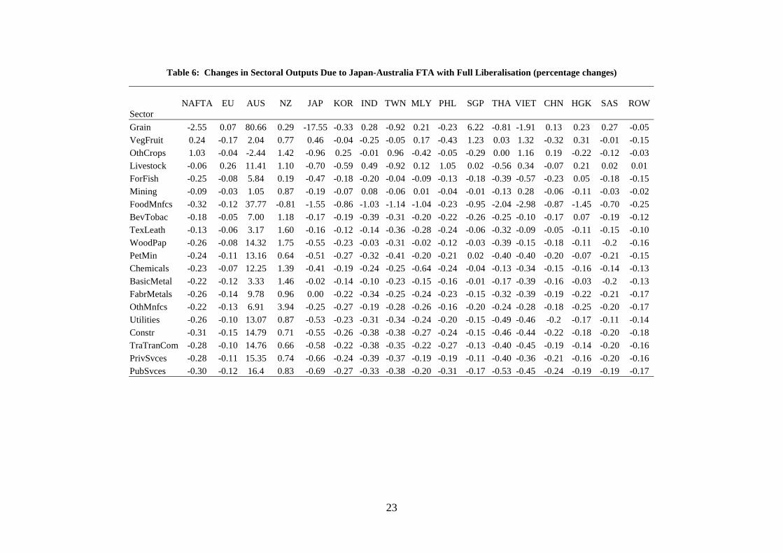
Table 6 reports the sectoral output responses to the FTA being implemented in its full

bilateral tariff elimination form between Australia and Japan. As tariff barriers disappear,

Australia is likely to experience substantial structural changes in terms of sectoral outputs in

comparison to Japan. Except for the “Other Crops” sector, all other sectors increase their

outputs in Australia. The most significant increases in outputs are recorded in “Grains” (80.7

per cent), and “Food Manufactures” (37.8 per cent). In essence, many sectors in the

Australian economy experience a balanced stimulation from free trade with Japan. While this

is undoubtedly good news for Australia, the output changes at sectoral level for Japan are

consistently negative, although the magnitudes of change are quite small in comparison to

Australian industry responses. Only Japanese sector that has experienced an increase in

output is “Vegetables and Fruit”.

19

Table 5: Decomposition of the Welfare Effects of the Japan-Australia FTA (US$ million)

Full Trade Liberalisation Scenario Trade Liberalisation Excluding Agriculture Scenario

`

Allocative Efficiency

(1)

Endowment Effect

(2)

Terms of Trade Effect

(3)

Capital Goods Effect

(4)

Equivalent Variation (EV)

(5)

Allocative Efficiency

(6)

Endowmen Effect

(7)

Terms of Trade Effect

(8)

Capital Goods Effect

(9)

Equivalent Variation (EV)

(10)

NAFTA -123.9 -22558.5 -432.3 -70.8 -23185.5 -289.6 -16748.2 -69.8 -25.0 -17132.5 EU -997.1 -6576.3 -117.4 38.1 -7652.6 -892.6 -6313.6 -58.2 10.0 -7254.4 AUS 5058.8 45760 3987.6 -2.7 54803.6 4344.5 38924.2 1404.9 -3.0 44670.6 NZ 64.9 388.7 -6.2 0.0 447.4 28.1 168.2 -1.8 -0.1 194.3 JAP -2065.1 -18703.4 -2516.9 80.2 -23205.2 -2517.1 -12166 -685.6 36.7 -15332 KOR -96.6 -804.4 -49.7 0.8 -949.8 -156.2 -814.3 -36.2 -0.1 -1006.7 IND -17.3 -487.2 -136 -0.4 -641 -12.7 -398.8 -62.7 -0.3 -474.4 TWN -96.7 -885.1 -38.6 10.9 -1009.6 -86.3 -810.1 -29.7 2.2 -923.9 MLY -26.8 -153.8 -21.4 0.2 -201.8 -15.7 -89.5 -16.9 0.4 -121.7 PHL -23.8 -124.6 -30.1 -6.9 -185.4 -19.7 -115.4 -19.7 -3.3 -158.1 SGP -10.4 -79.2 -23.1 -2.0 -114.8 -8.6 -57.3 -8.2 -0.7 -74.8 THA -89.8 -515.8 -80.4 1.2 -684.8 -87.4 -478.5 -84.7 0.4 -650.3 VIET -11.4 -61.0 -1.6 -0.4 -74.3 -15.1 -76.0 -6.7 0.4 -97.5 CHN -397.7 -1155.1 -180.2 13 -1720 -289.2 -1008.3 -126.2 5.6 -1418.1 HGK -0.9 -193.8 3.8 -21.9 -212.8 -0.7 -185.7 -3.5 -9.0 -198.9 SAS -147.6 -516.8 -163.5 -3.6 -831.6 -118.4 -531.2 -80.5 -1.6 -731.6 ROW -815.0 -4899.3 -201.4 -35.7 -5951.4 -661.0 -4350.3 -115.3 -12.6 -5139.2

20

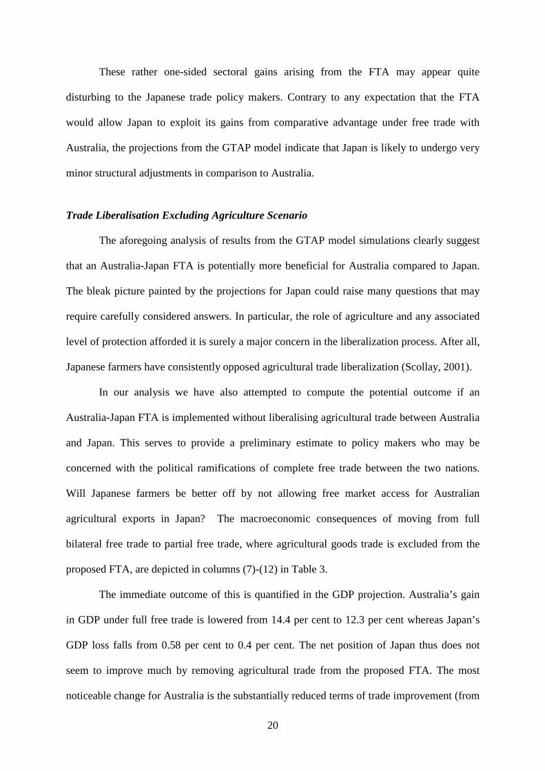
These rather one-sided sectoral gains arising from the FTA may appear quite

disturbing to the Japanese trade policy makers. Contrary to any expectation that the FTA

would allow Japan to exploit its gains from comparative advantage under free trade with

Australia, the projections from the GTAP model indicate that Japan is likely to undergo very

minor structural adjustments in comparison to Australia.

Trade Liberalisation Excluding Agriculture Scenario

The aforegoing analysis of results from the GTAP model simulations clearly suggest

that an Australia-Japan FTA is potentially more beneficial for Australia compared to Japan.

The bleak picture painted by the projections for Japan could raise many questions that may

require carefully considered answers. In particular, the role of agriculture and any associated

level of protection afforded it is surely a major concern in the liberalization process. After all,

Japanese farmers have consistently opposed agricultural trade liberalization (Scollay, 2001).

In our analysis we have also attempted to compute the potential outcome if an

Australia-Japan FTA is implemented without liberalising agricultural trade between Australia

and Japan. This serves to provide a preliminary estimate to policy makers who may be

concerned with the political ramifications of complete free trade between the two nations.

Will Japanese farmers be better off by not allowing free market access for Australian

agricultural exports in Japan? The macroeconomic consequences of moving from full

bilateral free trade to partial free trade, where agricultural goods trade is excluded from the

proposed FTA, are depicted in columns (7)-(12) in Table 3.

The immediate outcome of this is quantified in the GDP projection. Australia’s gain

in GDP under full free trade is lowered from 14.4 per cent to 12.3 per cent whereas Japan’s

GDP loss falls from 0.58 per cent to 0.4 per cent. The net position of Japan thus does not

seem to improve much by removing agricultural trade from the proposed FTA. The most

noticeable change for Australia is the substantially reduced terms of trade improvement (from

21

5.1 to 1.8 per cent) and the associated trade outcome. Consistent with the terms of trade

effect, Australia is likely import less than before and the projected trade surplus appears to be

23

Table 6: Changes in Sectoral Outputs Due to Japan-Australia FTA with Full Liberalisation (percentage changes)

Sector

NAFTA

EU

AUS

NZ

JAP

KOR

IND

TWN

MLY

PHL

SGP

THA

VIET

CHN

HGK

SAS

ROW

Grain -2.55 0.07 80.66 0.29 -17.55 -0.33 0.28 -0.92 0.21 -0.23 6.22 -0.81 -1.91 0.13 0.23 0.27 -0.05 VegFruit 0.24 -0.17 2.04 0.77 0.46 -0.04 -0.25 -0.05 0.17 -0.43 1.23 0.03 1.32 -0.32 0.31 -0.01 -0.15 OthCrops 1.03 -0.04 -2.44 1.42 -0.96 0.25 -0.01 0.96 -0.42 -0.05 -0.29 0.00 1.16 0.19 -0.22 -0.12 -0.03 Livestock -0.06 0.26 11.41 1.10 -0.70 -0.59 0.49 -0.92 0.12 1.05 0.02 -0.56 0.34 -0.07 0.21 0.02 0.01 ForFish -0.25 -0.08 5.84 0.19 -0.47 -0.18 -0.20 -0.04 -0.09 -0.13 -0.18 -0.39 -0.57 -0.23 0.05 -0.18 -0.15 Mining -0.09 -0.03 1.05 0.87 -0.19 -0.07 0.08 -0.06 0.01 -0.04 -0.01 -0.13 0.28 -0.06 -0.11 -0.03 -0.02 FoodMnfcs -0.32 -0.12 37.77 -0.81 -1.55 -0.86 -1.03 -1.14 -1.04 -0.23 -0.95 -2.04 -2.98 -0.87 -1.45 -0.70 -0.25 BevTobac -0.18 -0.05 7.00 1.18 -0.17 -0.19 -0.39 -0.31 -0.20 -0.22 -0.26 -0.25 -0.10 -0.17 0.07 -0.19 -0.12 TexLeath -0.13 -0.06 3.17 1.60 -0.16 -0.12 -0.14 -0.36 -0.28 -0.24 -0.06 -0.32 -0.09 -0.05 -0.11 -0.15 -0.10 WoodPap -0.26 -0.08 14.32 1.75 -0.55 -0.23 -0.03 -0.31 -0.02 -0.12 -0.03 -0.39 -0.15 -0.18 -0.11 -0.2 -0.16 PetMin -0.24 -0.11 13.16 0.64 -0.51 -0.27 -0.32 -0.41 -0.20 -0.21 0.02 -0.40 -0.40 -0.20 -0.07 -0.21 -0.15 Chemicals -0.23 -0.07 12.25 1.39 -0.41 -0.19 -0.24 -0.25 -0.64 -0.24 -0.04 -0.13 -0.34 -0.15 -0.16 -0.14 -0.13 BasicMetal -0.22 -0.12 3.33 1.46 -0.02 -0.14 -0.10 -0.23 -0.15 -0.16 -0.01 -0.17 -0.39 -0.16 -0.03 -0.2 -0.13 FabrMetals -0.26 -0.14 9.78 0.96 0.00 -0.22 -0.34 -0.25 -0.24 -0.23 -0.15 -0.32 -0.39 -0.19 -0.22 -0.21 -0.17 OthMnfcs -0.22 -0.13 6.91 3.94 -0.25 -0.27 -0.19 -0.28 -0.26 -0.16 -0.20 -0.24 -0.28 -0.18 -0.25 -0.20 -0.17 Utilities -0.26 -0.10 13.07 0.87 -0.53 -0.23 -0.31 -0.34 -0.24 -0.20 -0.15 -0.49 -0.46 -0.2 -0.17 -0.11 -0.14 Constr -0.31 -0.15 14.79 0.71 -0.55 -0.26 -0.38 -0.38 -0.27 -0.24 -0.15 -0.46 -0.44 -0.22 -0.18 -0.20 -0.18 TraTranCom -0.28 -0.10 14.76 0.66 -0.58 -0.22 -0.38 -0.35 -0.22 -0.27 -0.13 -0.40 -0.45 -0.19 -0.14 -0.20 -0.16 PrivSvces -0.28 -0.11 15.35 0.74 -0.66 -0.24 -0.39 -0.37 -0.19 -0.19 -0.11 -0.40 -0.36 -0.21 -0.16 -0.20 -0.16 PubSvces -0.30 -0.12 16.4 0.83 -0.69 -0.27 -0.33 -0.38 -0.20 -0.31 -0.17 -0.53 -0.45 -0.24 -0.19 -0.19 -0.17

24

Table 7: Changes in Sectoral Outputs Due to Japan-Australia FTA with Trade Liberalisation excluding Agriculture (percentage changes)

Sector

NAFTA

EU

AUS

NZ

JAP

KOR

IND

TWN

MLY

PHL

SGP

THA

VIET

CHN

HGK

SAS

ROW

Grain -0.17 0.02 -0.25 -0.37 -2.26 -0.38 -0.29 -0.71 -0.06 -0.25 1.45 -1.31 -2.27 -0.17 -0.19 0.02 -0.04 VegFruit -0.15 -0.09 -0.78 0.66 -0.10 0.03 -0.09 0.04 0.05 -0.14 0.51 0.15 0.82 -0.24 0.11 -0.04 -0.10 OthCrops 0.07 -0.07 4.07 0.91 -0.78 0.21 0.25 0.39 -0.05 -0.16 -0.11 0.11 1.53 0.14 0.02 -0.07 -0.02 Livestock -0.30 0.10 24.29 0.39 -2.37 -0.69 0.34 -0.72 0.07 0.46 0.03 -0.73 0.39 -0.06 0.10 0.00 -0.06 ForFish -0.27 -0.08 5.40 -0.01 -0.89 -0.23 -0.16 -0.09 -0.11 -0.12 -0.13 -0.40 -0.65 -0.22 0.02 -0.16 -0.17 Mining -0.05 -0.01 0.96 0.71 -0.08 -0.05 0.09 -0.04 0.03 0.00 0.02 -0.11 0.25 -0.03 -0.10 -0.02 0.00 FoodMnfcs -0.49 -0.16 51.52 -1.32 -3.23 -0.98 -0.85 -1.39 -0.84 -0.35 -1.22 -2.12 -3.13 -0.89 -1.51 -0.63 -0.29 BevTobac -0.18 -0.09 9.35 0.50 -0.20 -0.19 -0.26 -0.27 -0.12 -0.23 -0.19 -0.24 -0.27 -0.13 -0.08 -0.14 -0.11 TexLeath -0.15 -0.08 5.08 1.20 -0.07 -0.16 -0.06 -0.35 -0.14 -0.18 -0.06 -0.22 -0.08 0.00 -0.11 -0.05 -0.10 WoodPap -0.21 -0.08 12.69 1.26 -0.45 -0.24 0.00 -0.28 0.05 -0.10 -0.01 -0.36 -0.17 -0.14 -0.11 -0.18 -0.14 PetMin -0.17 -0.10 11.30 0.25 -0.33 -0.26 -0.25 -0.37 -0.11 -0.19 0.03 -0.37 -0.46 -0.16 -0.06 -0.18 -0.13 Chemicals -0.16 -0.07 11.11 0.93 -0.21 -0.20 -0.16 -0.23 -0.13 -0.20 -0.02 -0.05 -0.40 -0.12 -0.16 -0.12 -0.12 BasicMetal -0.17 -0.11 2.95 1.14 0.07 -0.14 -0.05 -0.20 -0.10 -0.14 0.01 -0.14 -0.42 -0.13 -0.01 -0.16 -0.11 FabrMetals -0.20 -0.13 8.45 0.48 0.10 -0.21 -0.25 -0.22 -0.15 -0.18 -0.12 -0.27 -0.40 -0.15 -0.19 -0.18 -0.15 OthMnfcs -0.15 -0.11 6.10 3.09 -0.27 -0.22 -0.07 -0.19 -0.12 -0.04 -0.12 -0.11 -0.24 -0.10 -0.16 -0.16 -0.14 Utilities -0.19 -0.10 11.30 0.44 -0.39 -0.23 -0.23 -0.32 -0.14 -0.19 -0.11 -0.46 -0.55 -0.17 -0.16 -0.13 -0.13 Constr -0.23 -0.14 12.77 0.29 -0.37 -0.26 -0.28 -0.34 -0.14 -0.21 -0.11 -0.41 -0.52 -0.18 -0.16 -0.18 -0.16 TraTranCom -0.21 -0.09 12.50 0.27 -0.39 -0.21 -0.27 -0.32 -0.12 -0.23 -0.07 -0.35 -0.50 -0.15 -0.13 -0.17 -0.13 PrivSvces -0.21 -0.10 12.81 0.31 -0.44 -0.24 -0.30 -0.33 -0.11 -0.16 -0.08 -0.37 -0.47 -0.17 -0.15 -0.17 -0.14 PubSvces -0.22 -0.11 13.31 0.36 -0.45 -0.28 -0.28 -0.35 -0.13 -0.27 -0.11 -0.51 -0.60 -0.21 -0.18 -0.19 -0.15

25

lower than under full free trade. The reduced welfare gain as measured by the EV is the net

effect of the exclusion of agricultural goods from the free trade agreement.

Turning to the rest of the macroeconomic results for Japan in Table 3, the

deterioration of the terms of trade is now less than before, but the trade results (exports and

imports) remain more or less the same. However, the projected trade deficit is substantially

reduced as a consequence of the less severe deterioration in the terms of trade. The loss in

welfare (as shown by the EV) is also substantially reduced. All in all, the results suggest that

the exclusion of agricultural trade from the FTA does not improve the economic outcome for

Japan. Indeed, the severity of some of the negative effects may be somewhat reduced.

On examining the projections of demand for labour and capital in Table 4, and the

welfare decomposition in Table 5, it is possible to come to a similar conclusion. For

Australia, the positive effects observed under full bilateral liberalization are reduced

marginally in the event of the exclusion of agriculture from the proposed FTA whereas, for

Japan, the magnitude of the negative impact declines.

Sectoral output projections reported in Table 7 indicate how both Australian and

Japanese producers respond to the exclusion of agricultural trade from the proposed FTA.

The stimulus provided to Australian agriculture is greatly reduced and sectors like “Grains”

and “Vegetable and fruits” show decline in outputs. However, sectors such as “Other crops”,

“Livestock”, “Food manufacturing”, “Beverages and tobacco”, and “Textile and leather”

perform better than before. For Japan, the outcome is still not as good as one would expect

given the unusually heavy protection afforded the agricultural sectors. The highly protected

“Grains” sector in Japan still shows a decline in output and the previous marginal gain

experienced by the “Vegetable and fruit” sector has now been reversed. Many other sectors in

Japan undergo output changes that are very small in magnitude. In sum, it thus seems that the

26

exclusion of agricultural goods from the FTA has not changed the option (i) results

significantly.

7 Concluding Remarks

The proposed Australia-Japan FTA is likely to generate a heated debate amongst the

Pacific community of nations. Economists can play a positive role in this debate by providing

carefully modelled estimates of the economic magnitudes involved. Accordingly, we have

sought to contribute some preliminary findings on the probable impact of the proposed

Australia-Japan FTA using the GTAP multicountry CGE model. Two different plausible

alternative scenarios were examined: full free trade and full free trade without agricultural

goods.

A number of informative conclusions can be drawn from our estimates. In the first

place, under full free trade, Australia will benefit substantially in terms of both GDP and

welfare projections. Australian exports to and imports from Japan will increase markedly and

its improved terms of trade will yield a larger trade surplus. By contrast, Japanese economic

performance under full free trade is not favourable in aggregate. Its trade deficit will increase

and GDP will fall. Secondly, the exclusion of agricultural goods from the proposed FTA will

improve Japanese economic prospects only marginally, but still result in an overall negative

outcome.

These conclusions should not perplex trade negotiators. After all, since the Japanese

economy dwarves its Australian counterpart, it is not surprising that bilateral trade

liberalisation should have a comparatively small impact on Japan and a significant effect on

Australia. While Australia will experience considerable structural change, Japanese sectoral

output responses are almost negligible, except in the politically sensitive case of agriculture.

27

Policymakers should thus embrace the fact that Australia has much to gain and Japanese non-

agricultural producers very little to lose from an Australia-Japan FTA.

28

References Bhagwati, J. and Panagariya, A. (eds.) (1996), The Economics of Preferential Trade Agreements, AEI Press, Washington. Dimaranan, B. V. and McDougall, R. A. (2002), Global Trade, Assistance, and Production: The GTAP 5 Data Base, Centre for Global Trade Analysis, Purdue University, U.S.A. Dixon, P. B., Parmenter, B. R., Sutton, J. and Vincent, D.P. (1982), ORANI: Multisectoral Model of the Australian Economy, Amsterdam, North-Holland. Estevadeordal, A. (2000), “Negotiating Preferential Market Access: The Case of the North American Free Trade Agreement”, Journal of World Trade, 34(1), pp. 141-166. Hertel, T. W. (1996), Global Trade Analysis: Modelling and Applications, New York and Cambridge, Cambridge University Press. International Monetary Fund, Direction of Trade Statistics Yearbook, various issues. Petri, P. (1997), “Computable General Equilibrium Studies of APEC: Preliminary Overview”, unpublished mimeo, Brandeis University. Scollay, R. (2001), “The Changing Outlook for Asia-Pacific Regionalism”, World Economy, 24(9), pp.1135-1160. Scollay, R. and Gilbert, J. (2000), “Measuring the Gains from APEC Liberalisation: An Overview”, World Economy, 23(2), pp.175-198. Siriwardana, M. (2001), “Looking Beyond SAARC: Some Trade Liberalisation Options for Sri Lanka”, Asian Studies Review, 25(4): pp.453-478. Viner, J. (1950), The Customs Union Issue, Carnegie Endowment for International Peace, New York.

29

Appendix Table A1: Regional and Commodity Aggregation Aggregated Region

GTAP Region Aggregated Commodity GTAP Commodity

1. North American Free Trade Area (NAFTA)

U.S.A. Canada Mexico

1. Grains Paddy rice, wheat, cereal grains nec

2. European Union (EU) 3. Australia (AUS)

United Kingdom Germany Denmark Sweden Finland Rest of European Union Australia

2. Vegetables and Fruits 3. Other Crops 4. Animals and animal products

Vegetables, Fruits, Nuts, Oil seeds Sugar cane, Sugar beet, Plant-based fibers, Crops nec Cattle, sheep, goat, horses, Animal products nec, Raw milk, Wool, silk-worm cocoons

4. New Zealand (NZ) New Zealand

5. Forestry and Fishing Forestry, Fishing

5. Japan (JAP) Japan

6. Minerals Coal, Oil, Gas, Minerals nec

6. Korea (KOR) 7. Indonesia (IND 8. Taiwan (TWN)

Korea Indonesia Taiwan

7. Food manufactures Meat: cattle, sheep, goats, horse; Meat products nec, Vegetable oil and fats, Dairy products, Processed rice, Sugar, Food products nec

9. Malaysia (MLY)

Malaysia

8. Beverages and Tobacco

Beverages and tobacco products

10. Philippines (PHL) Philippines 11. Singapore (SGP)

Singapore

9. Textiles and leather Textiles, Wearing apparel, Leather products

12. Thailand (THA)

Thailand

13. Vietnam (VIET)

Vietnam

10. Wood and Paper Products Wood products, Paper products, publishing

14. China (CHN) 15. Hong Kong (HGK)

China Hong Kong

11.Petroleum and other mineral products Petroleum, coal products, Mineral products nec

16. South Asia (SAS)

India Sri Lanka Bangladesh Rest of South Asia

12. Chemical, Rubber, Plastic Chemical, rubber, plastic prods

17. Rest of the World

All Other Regions

13. Basic metals Ferrous metals, metals nec

14. Fabricated Metal Products Metal products, Motor vehicles and parts, Transport equipment nec, Electronic equipment, Machinery and equipment nec

15. Other Manufactures Manufactures nec

16. Electricity, Gas, Water Electricity, Gas manufacture and distribution, Water

17. Construction Construction

18. Trade, Transport, Communication Trade, Sea transport, Air transport, Communication

19. Private Services Financial services nec, Insurance, Business services nec, Recreation and other services, Dwellings

20. Public Services PubAdmin/Defence/Health/Education

Source; Dimaranan and McDougall et al. ( 2002)