
An efficient 3D topology optimization code written in Matlab · An efficient 3D topology...
22
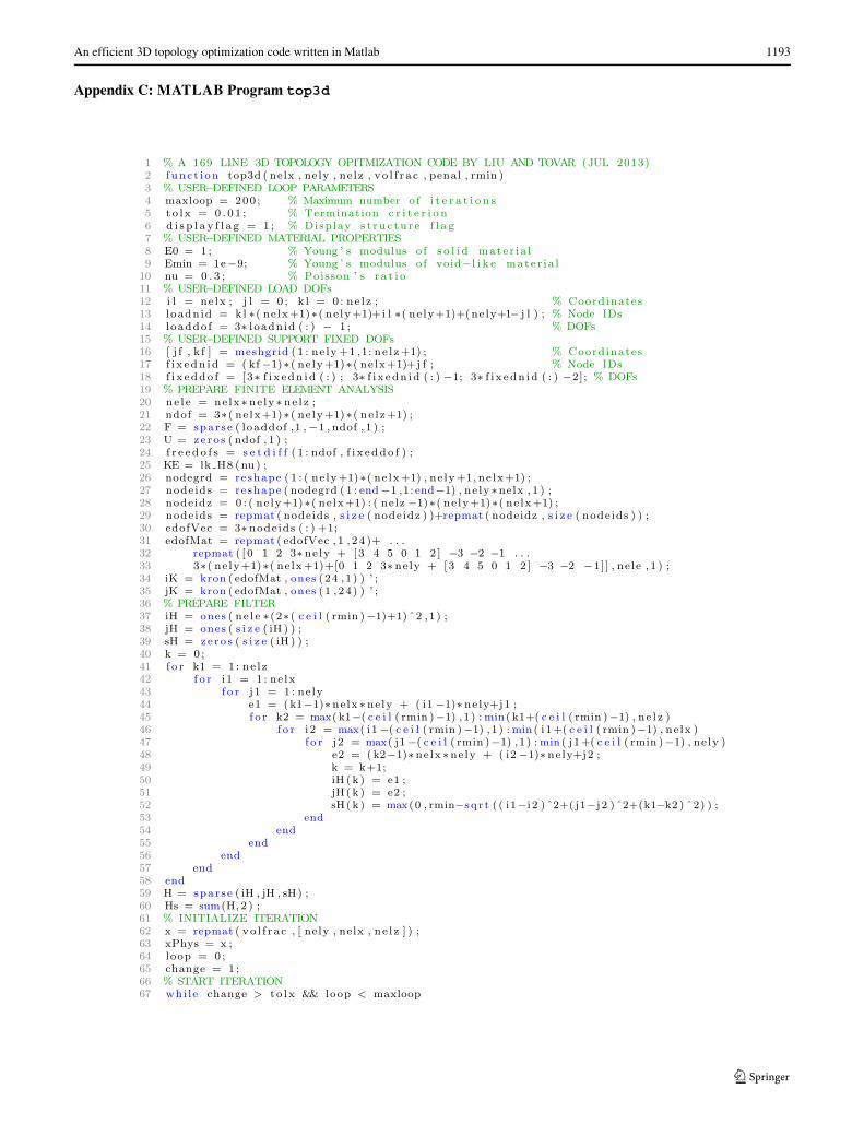
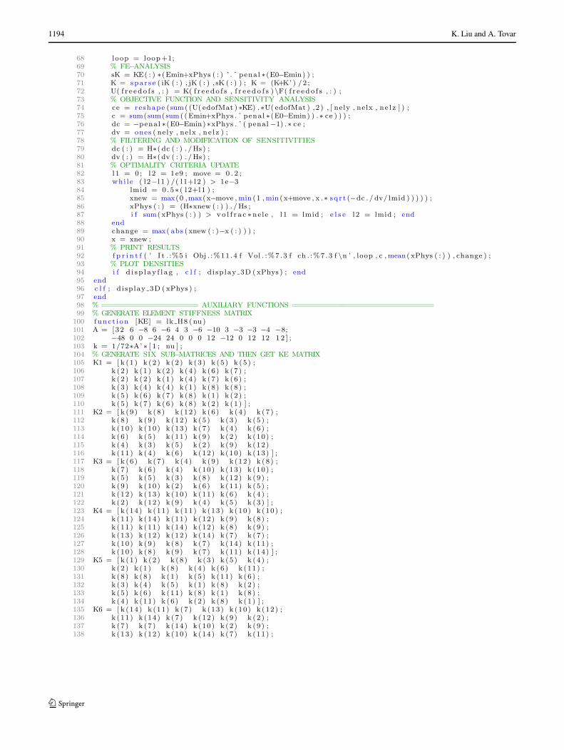
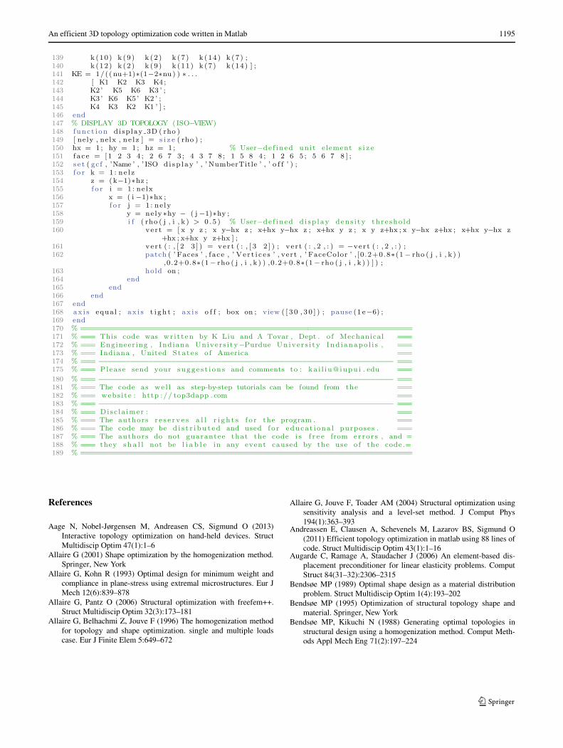
Struct Multidisc Optim (2014) 50:1175–1196 DOI 10.1007/s00158-014-1107-x EDUCATIONAL ARTICLE An efficient 3D topology optimization code written in Matlab Kai Liu · Andr´ es Tovar Received: 17 October 2013 / Revised: 19 March 2014 / Accepted: 22 April 2014 / Published online: 25 June 2014 © Springer-Verlag Berlin Heidelberg 2014 Abstract This paper presents an efficient and compact MATLAB code to solve three-dimensional topology opti- mization problems. The 169 lines comprising this code include finite element analysis, sensitivity analysis, density filter, optimality criterion optimizer, and display of results. The basic code solves minimum compliance problems. A systematic approach is presented to easily modify the defini- tion of supports and external loads. The paper also includes instructions to define multiple load cases, active and pas- sive elements, continuation strategy, synthesis of compliant mechanisms, and heat conduction problems, as well as the theoretical and numerical elements to implement general non-linear programming strategies such as SQP and MMA. The code is intended for students and newcomers in the topology optimization. The complete code is provided in Appendix C and it can be downloaded from http://top3dapp. com. Keywords Topology optimization · MATLAB · Compliance · Compliant mechanism · Heat conduction · Non-linear programming 1 Introduction Topology optimization is a computational material distribu- tion method for synthesizing structures without any precon- ceived shape. This freedom provides topology optimization K. Liu () · A. Tovar Department of Mechanical Engineering, Indiana University-Purdue University Indianapolis, Indianapolis, IN 46202, USA e-mail: [email protected] with the ability to find innovative, high-performance struc- tural layouts, which has attracted the interest of applied mathematicians and engineering designers. From the work of Lucien Schmit in the 1960s (Schmit 1960)—who recog- nized the potential of combining optimization methods with finite-element analysis for structural design—and the semi- nal paper by Bendsøe and Kikuchi (1988), there have been more than eleven thousand journal publications in this area (Compendex list as of September 2013), several reference books (Hassani and Hinton 1998; Bendsøe and Sigmund 2003; Christensen and Klarbring 2009), and a number of readily available educational computer tools for MATLAB and other platforms. Some examples of such tools include the topology optimization program by Liu et al. (2005) for Femlab, the shape optimization program by Allaire and Pantz (2006) for FreeFem++, the open source topology optimization program ToPy by Hunter (2009) for Python, and the 99-line program for Michell-like truss structures by Sok´ ol (2011) for Mathematica. For MATLAB, Sigmund (2001) introduced the 99-line program for two-dimensional topology optimization. This program uses stiffness matrix assembly and filtering via nested loops, which makes the code readable and well- organized but also makes it slow when solving larger problems. Andreassen et al. (2011) presented the 88-line program with improved assembly and filtering strategies. When compared to the 99-line code in a benchmark prob- lem with 7500 elements, the 88-line code is two orders of magnitude faster. From the same research group, Aage et al. (2013) introduced TopOpt, the first topology optimization App for hand-held devices. Also for MATLAB, Wang et al. (2004) introduced the 199-line program TOPLSM making use of the level-set method. Challis (2010) also used the level-set method but with discrete variables in a 129-line program. Suresh (2010)
Transcript of An efficient 3D topology optimization code written in Matlab · An efficient 3D topology...

Struct Multidisc Optim (2014) 50:1175–1196DOI 10.1007/s00158-014-1107-x
EDUCATIONAL ARTICLE
An efficient 3D topology optimization code written in Matlab
Kai Liu · Andres Tovar
Received: 17 October 2013 / Revised: 19 March 2014 / Accepted: 22 April 2014 / Published online: 25 June 2014© Springer-Verlag Berlin Heidelberg 2014
Abstract This paper presents an efficient and compactMATLAB code to solve three-dimensional topology opti-mization problems. The 169 lines comprising this codeinclude finite element analysis, sensitivity analysis, densityfilter, optimality criterion optimizer, and display of results.The basic code solves minimum compliance problems. Asystematic approach is presented to easily modify the defini-tion of supports and external loads. The paper also includesinstructions to define multiple load cases, active and pas-sive elements, continuation strategy, synthesis of compliantmechanisms, and heat conduction problems, as well as thetheoretical and numerical elements to implement generalnon-linear programming strategies such as SQP and MMA.The code is intended for students and newcomers in thetopology optimization. The complete code is provided inAppendix C and it can be downloaded from http://top3dapp.com.
Keywords Topology optimization · MATLAB ·Compliance · Compliant mechanism · Heat conduction ·Non-linear programming
1 Introduction
Topology optimization is a computational material distribu-tion method for synthesizing structures without any precon-ceived shape. This freedom provides topology optimization
K. Liu (�) · A. TovarDepartment of Mechanical Engineering,Indiana University-Purdue University Indianapolis,Indianapolis, IN 46202, USAe-mail: [email protected]
with the ability to find innovative, high-performance struc-tural layouts, which has attracted the interest of appliedmathematicians and engineering designers. From the workof Lucien Schmit in the 1960s (Schmit 1960)—who recog-nized the potential of combining optimization methods withfinite-element analysis for structural design—and the semi-nal paper by Bendsøe and Kikuchi (1988), there have beenmore than eleven thousand journal publications in this area(Compendex list as of September 2013), several referencebooks (Hassani and Hinton 1998; Bendsøe and Sigmund2003; Christensen and Klarbring 2009), and a number ofreadily available educational computer tools for MATLAB
and other platforms. Some examples of such tools includethe topology optimization program by Liu et al. (2005) forFemlab, the shape optimization program by Allaire andPantz (2006) for FreeFem++, the open source topologyoptimization program ToPy by Hunter (2009) for Python,and the 99-line program for Michell-like truss structures bySokoł (2011) for Mathematica.
For MATLAB, Sigmund (2001) introduced the 99-lineprogram for two-dimensional topology optimization. Thisprogram uses stiffness matrix assembly and filtering vianested loops, which makes the code readable and well-organized but also makes it slow when solving largerproblems. Andreassen et al. (2011) presented the 88-lineprogram with improved assembly and filtering strategies.When compared to the 99-line code in a benchmark prob-lem with 7500 elements, the 88-line code is two orders ofmagnitude faster. From the same research group, Aage et al.(2013) introduced TopOpt, the first topology optimizationApp for hand-held devices.
Also for MATLAB, Wang et al. (2004) introduced the199-line program TOPLSM making use of the level-setmethod. Challis (2010) also used the level-set method butwith discrete variables in a 129-line program. Suresh (2010)

1176 K. Liu and A. Tovar
presented a 199-line program ParetoOptimalTracingthat traces the Pareto front for different volume fractionsusing topological sensitivities. More recently, Talischi et al.(2012a, b) introduced PolyMesher and PolyTop fordensity-based topology optimization using polygonal finiteelements. The use of polygonal elements makes these pro-grams suitable for arbitrary non-Cartesian design domainsin two dimensions.
One of the few contributions to three-dimensional MAT-LAB programs is presented by Zhou and Wang (2005). Thiscode, referred to as the 177-line program, is a successorto the 99-line program by Sigmund (2001) that inheritsand amplifies the same drawbacks. Our paper presents a169-line program referred to as top3d that incorporatesefficient strategies for three-dimensional topology opti-mization. This program can be effectively used in personalcomputers to generate structures of substantial size. Thispaper explains the use of top3d in minimum compli-ance, compliant mechanism, and heat conduction topologyoptimization problems.
The rest of this paper is organized as follows. Section 2briefly reviews theoretical aspects in topology optimiza-tion with focus on the density-based approach. Section 3introduces 3D finite element analysis and its numericalimplementation. Section 4 presents the formulation of threetypical topology optimization problems, namely, minimumcompliance, compliant mechanism, and heat conduction.Section 5 discusses the optimization methods and theirimplementation in the code. Section 6 shows the numer-ical implementation procedures and results of three dif-ferent topology optimization problems, several extensionsof the top3d code, and multiple alternative implementa-tions. Finally, Section 7, offers some closing thoughts. Thetop3d code is provided in Appendix C and can also bedownloaded for free from the website: http://top3dapp.com.
2 Theoretical background
2.1 Problem definition and ill-posedness
A topology optimization problem can be defined as a binaryprogramming problem in which the objective is to findthe distribution of material in a prescribed area or volumereferred to as the design domain. A classical formulation,referred to as the binary compliance problem, is to find the“black and white” layout (i.e., solids and voids) that min-imizes the work done by external forces (or compliance)subject to a volume constraint.
The binary compliance problem is known to be ill-posed(Kohn and Strang 1986a, b, c). In particular, it is possibleto obtain a non-convergent sequence of feasible black-and-white designs that monotonically reduce the structure’s
compliance. As an illustration, assume that a design hasone single hole. Then, it is possible to find an improvedsolution with the same mass and lower compliance whenthis hole is replaced by two smaller holes. Improved solu-tions can be successively found by increasing the numberof holes and reducing their size. The design will progresstowards a chattering design within infinite number of holesof infinitesimal size. That makes the compliance problemunbounded and, therefore, ill-posed.
One alternative to make the compliance problem well-posed is to control the perimeter of the structure (Haber andJog 1996; Jog 2002). This method effectively avoids chat-tering configurations, but its implementation is not free ofcomplications. It has been reported that the addition of aperimeter constraint creates fluctuations during the iterativeoptimization process so internal loops need to be incorpo-rated (Duysinx 1997) Op. cit. (Bendsøe and Sigmund 2003).Also, small variations in the parameters of the algorithmlead to dramatic changes in the final layout (Jog 2002).
2.2 Homogenization method
Another alternative is to relax the binary condition andinclude intermediate material densities in the problem for-mulation. In this way, the chattering configurations becomepart of the problem statement by assuming a periodicallyperforated microstructure. The mechanical properties of thematerial are determined using the homogenization theory.This method is referred to as the homogenization methodfor topology optimization (Bendsøe 1995; Allaire 2001).The main drawback of this approach is that the optimalmicrostructure, which is required in the derivation of therelaxed problem, is not always known. This can be allevi-ated by restricting the method to a subclass of microstruc-tures, possibly suboptimal but fully explicit. This approach,referred to as partial relaxation, has been utilized by manyauthors including Bendsøe and Kikuchi (1988), Allaireand Kohn (1993), Allaire et al. (2004), and referencestherein.
An additional problem with the homogenization meth-ods is the manufacturability of the optimized structure.The “gray” areas found in the final designs contain micro-scopic length-scale holes that are difficult or impossibleto fabricate. However, this problem can be mitigated withpenalization strategies. One approach is to post-process thepartially relaxed optimum and force the intermediate den-sities to take black or white values (Allaire et al. 1996).This a posteriori procedure results in binary designs, but itis purely numerical and mesh dependent. Other approachis to impose a priori restrictions on the microstructure thatimplicitly lead to black-and-white designs (Bendsøe 1995).Even though penalization methods have shown to be effec-tive in avoiding or mitigating intermediate densities, they

An efficient 3D topology optimization code written in Matlab 1177
revert the problem back to the original ill-possedness withrespect to mesh refinement.
2.3 Density-based approach
An alternative that avoids the application of homogenizationtheory is to relax the binary problem using a continu-ous density value with no microstructure. In this method,referred to as the density-based approach, the material dis-tribution problem is parametrized by the material densitydistribution. In a discretized design domain, the mechan-ical properties of the material element, i.e., the stiffnesstensor, are determined using a power-law interpolation func-tion between void and solid (Bendsøe 1989; Mlejnek 1992).The power law may implicitly penalize intermediate densityvalues driving the structure towards a black-and-white con-figuration. This penalization procedure is usually referredto as the Solid Isotropic Material with Penalization (SIMP)method (Zhou and Rozvany 1991). The SIMP method doesnot solve the problem’s ill-possedness, but it is simpler thanother penalization methods.
The SIMP method is based on a heuristic relationbetween (relative) element density xi and element Young’smodulus Ei given by
Ei = Ei(xi) = xp
i E0, xi ∈]0, 1], (1)
where E0 is the elastic modulus of the solid material and p isthe penalization power (p > 1). A modified SIMP approachis given by
Ei = Ei(xi) = Emin + xpi (E0 − Emin), xi ∈ [0, 1], (2)
where Emin is the elastic modulus of the void material,which is non-zero to avoid singularity of the finite elementstiffness matrix. The modified SIMP approach, as (2), offersa number of advantages over the classical SIMP formula-tion, as shown in (1), including the independency betweenthe minimum value of the material’s elastic modulus and thepenalization power (Sigmund 2007).
However, topology optimization methods are likely toencounter numerical difficulties such as mesh-dependency,checkerboard patterns, and local minima (Bendsøe andSigmund 2003). In order to mitigate such issues, resear-chers have proposed the use of regularization techniques(Sigmund and Peterson 1998). One of the most commonapproaches is the use of density filters (Bruns and Tortorelli2001). A basic filter density function is defined as
xi =∑
j∈NiHij vjxj
∑j∈Ni
Hij vj
, (3)
where Ni is the neighborhood of an element xi with volumevi , and Hij is a weight factor. The neighborhood is definedas
Ni = {j : dist(i, j) � R} , (4)
where the operator dist(i, j ) is the distance between the cen-ter of element i and the center of element j , and R is thesize of the neighborhood or filter size. The weight factorHij may be defined as a function of the distance betweenneighboring elements, for example
Hij = R − dist(i, j), (5)
where j ∈ Ni . The filtered density xi defines a modi-fied (physical) density field that is now incorporated in thetopology optimization formulation and the SIMP model as
Ei (xi) = Emin + xpi (E0 − Emin), xi ∈ [0, 1]. (6)
The regularized SIMP interpolation formula defined by (6)used in this work.
3 Finite element analysis
3.1 Equilibrium equation
Following the regularized SIMP method given by (6) andthe generalized Hooke’s law, the three-dimensional consti-tutive matrix for an isotropic element i is interpolated fromvoid to solid as
Ci (xi) = Ei (xi)C0i , xi ∈ [0, 1], (7)
where C0i is the constitutive matrix with unit Young’s
modulus. The unit constitutive matrix is given by
C0i = 1
(1 + ν)(1 − 2ν)×
⎡
⎢⎢⎢⎢⎣
1 − ν ν ν 0 0 0ν 1 − ν ν 0 0 0ν ν 1 − ν 0 0 00 0 0 (1 − 2ν)/2 0 00 0 0 0 (1 − 2ν)/2 00 0 0 0 0 (1 − 2ν)/2
⎤
⎥⎥⎥⎥⎦
, (8)
where ν is the Poisson’s ratio of the isotropic material.Using the finite element method, the elastic solid elementstiffness matrix is the volume integral of the elements con-stitutive matrix Ci(xi ) and the strain–displacement matrixB in the form of
ki (xi) =∫ +1
−1
∫ +1
−1
∫ +1
−1BTCi(xi )Bdξ1dξ2dξ3, (9)
where ξe (e = 1, . . . , 3) are the natural coordinates asshown in Fig. 1, and the hexahedron coordinates of the cor-ners are shown in Table 1. The strain–displacement matrixB relates the strain ε and the nodal displacement u, ε = Bu.Using the SIMP method, the element stiffness matrix isinterpolated as
ki (xi) = Ei (xi)k0i , (10)

1178 K. Liu and A. Tovar
1 2
34
5 6
78
ξ1
ξ2
ξ3
Fig. 1 The eight-node hexahedron and the natural coordinatesξ1, ξ2, ξ3
where
k0i =
∫ +1
−1
∫ +1
−1
∫ +1
−1BTC0Bdξ1dξ2dξ3. (11)
Replacing values in (11), the 24 × 24 element stiffnessmatrix k0
i for an eight-node hexahedral element is
k0i = 1
(ν + 1)(1 − 2ν)
⎡
⎢⎢⎣
k1 k2 k3 k4
kT2 k5 k6 kT
4kT
3 k6 kT5 kT
2k4 k3 k2 kT
1
⎤
⎥⎥⎦ (12)
where km (m = 1, . . . , 6) are 6×6 symmetric matrices (seeAppendix A). One can also verify that k0
i is positive definite.The global stiffness matrix K is obtained by the assemblyof element-level counterparts ki ,
K(x) = �ni=1ki (xi) = �
ni=1Ei (xi)k0
i , (13)
where n is the total number of elements. Using the globalversions of the element stiffness matrices Ki and K0
i , (13)is expressed as
K(x) =n∑
i=1
Ki(xi) =n∑
i=1
Ei(xi)K0i . (14)
Table 1 The eight-node hexahedral element with node numberingconventions
Node ξ1 ξ2 ξ3
1 −1 −1 −1
2 +1 −1 −1
3 +1 +1 −1
4 −1 +1 −1
5 −1 −1 +1
6 +1 −1 +1
7 +1 +1 +1
8 −1 +1 +1
where K0i is a constant matrix. Using the interpolation
function defined in (6), one finally observes that
K(x) =n∑
i=1
[Emin + xp
i (E0 − Emin)]
K0i . (15)
Finally, the nodal displacements vector U(x) is the solu-tion of the equilibrium equation
K(x)U(x) = F, (16)
where F is the vector of nodal forces and it is independentof the physical densities x. For brevity of notation, we omit-ted the dependence of physical densities x on the designvariables x, x = x(x).
3.2 Numerical implementation
Consider the discretized prismatic structure in Fig. 2 com-posed of eight eight-noded cubic elements. The nodesidentified with a number (node ID) ordered column-wiseup-to-bottom, left-to-right, and back-to-front. The positionof each node is defined with respect to Cartesian coordinatesystem with origin at the left-bottom-back corner.
Within each element, the eight nodes N1, . . . , N8 areordered in counter-clockwise direction as shown in Fig. 3.Note that the “local” node number (Ni) does not follow thesame rule as the “global” node ID (NIDi ) system in Fig. 2.Given the size of the volume (nelx× nely× nelz) andthe global coordinates of node N1 (x1, y1, z1), one can iden-tify the global node coordinates and node IDs of the otherseven nodes in that element by the mapping the relationshipsas summarized in Table 2.
Each node in the structure has three degrees of free-dom (DOFs) corresponding to linear displacements in x-y-zdirections (one element has 24 DOFs). The degrees of free-dom are organized in the nodal displacement vector Uas
U = [U1x, U1y, U1z, . . . , U8×nz
]T,
1
2
3
4
5
6
7
8
9
10
11
12
13
14
15
16
17
18
19
20
21
22
23
24
25
26
27
28
29
30
x
y
z
Fig. 2 Global node IDs in a prismatic structure composed of 8elements

An efficient 3D topology optimization code written in Matlab 1179
N1 N2
N4 N3
N8 N7
N5 N6
xy
z
Fig. 3 Local node numbers within a cubic element
where n is the number of elements in the structure. The loca-tion of the DOFs in U, and consequently K and F, can bedetermined from the node ID as shown in Table 2.
The node IDs for each element are organized in a con-nectivity matrix edofMat with following MATLAB lines:
where nele is the total number of elements, nodegrdcontains the node ID of the first grid of nodes in the x-yplane (for z = 0), the column vector edofVec containsthe node IDs of the first node at each element, and the con-nectivity matrix edofMat of size nele × 24 containing
the node IDs for each element. For the volume in Fig. 2,nelx = 4, nely = 1, and nelz = 2, which results in
edofMat =
⎡
⎢⎢⎢⎢⎢⎢⎢⎢⎢⎢⎣
4 5 6 · · · 31 32 3310 11 12 · · · 37 38 3916 17 18 · · · 43 44 4522 23 24 · · · 49 50 5134 35 36 · · · 61 62 6340 41 42 · · · 67 68 6946 47 48 · · · 73 74 7552 53 54 · · · 79 80 81
⎤
⎥⎥⎥⎥⎥⎥⎥⎥⎥⎥⎦
← Element 1← Element 2← Element 3← Element 4← Element 5← Element 6← Element 7← Element 8 .
The element connectivity matrix edofMat is used toassemble the global stiffness matrix K as follows:
The element stiffness matrix KE (size 24×24) is obtainedfrom the lk H8 subroutine (lines 99-146). Matrices iK(size 24 nele×24) and jK (size nele×242), reshaped ascolumn vectors, contain the rows and columns identifyingthe 24 × 24 × nele DOFs in the structure. The three-dimensional array xPhys (size nely × nelx × nelz)corresponds to the physical densities. The matrix sK (size242 × nele) contains all element stiffness matrices. Theassembly procedure of the (sparse symmetric) global stiff-ness matrix K (line 71) avoids the use of nested forloops.
Finally, the nodal displacement vector U is obtainedfrom the solution of the equilibrium equation (16) by pre-multiplying the inverse of the stiffness matrix K and thevector of nodal forces F,
Table 2 Illustration of relationships between node number, node coordinates, node ID and node DOFs
Node Number Node coordinates Node ID Node Degree of Freedoms
x y z
N1 (x1, y1, z1) NID†1 3 ∗ NID1 − 2 3 ∗ NID1 − 1 3 ∗ NID1
N2 (x1 + 1, y1, z1) NID2 = NID1 + (nely + 1) 3 ∗ NID2 − 2 3 ∗ NID2 − 1 3 ∗ NID2
N3 (x1 + 1, y1 + 1, z1) NID3 = NID1 + nely 3 ∗ NID3 − 2 3 ∗ NID3 − 1 3 ∗ NID3
N4 (x1, y1 + 1, z1) NID4 = NID1 − 1 3 ∗ NID4 − 2 3 ∗ NID4 − 1 3 ∗ NID4
N5 (x1, y1, z1 + 1) NID5 = NID1 + NID‡z 3 ∗ NID5 − 2 3 ∗ NID5 − 1 3 ∗ NID5
N6 (x1 + 1, y1, z1 + 1) NID6 = NID2 + NIDz 3 ∗ NID6 − 2 3 ∗ NID6 − 1 3 ∗ NID6
N7 (x1 + 1, y1 + 1, z1 + 1) NID7 = NID3 + NIDz 3 ∗ NID7 − 2 3 ∗ NID7 − 1 3 ∗ NID7
N8 (x1, y1 + 1, z1 + 1) NID8 = NID4 + NIDz 3 ∗ NID8 − 2 3 ∗ NID8 − 1 3 ∗ NID8
†NID1 = z1*(nelx+1)*(nely+1)+x1∗(nely+1)+(nely+1 − y1)
‡NIDz = (nelx+1)*(nely+1)

1180 K. Liu and A. Tovar
where the indices freedofs indicate the unconstrainedDOFs. For the cantilevered structure in Fig. 2, the con-strained DOFs
where jf, and kf are the coordinate of the fixed nodes,fixednid are the node IDs, and fixeddof are thelocation of the DOFs. The free DOFs, are then defined as
where ndof is the total number of DOFs. By default, thecode constraints the left face of the prismatic structure andassigns a vertical load to the structure’s free-lower edge asdepicted in Fig. 2. The user can define different load andsupport DOFs by changing the corresponding node coordi-nates (lines 12 and 16). Several examples are presented inSection 6.
4 Optimization problem formulation
Three representative topology optimization problems aredescribed in this section, namely: minimum compliance,compliant mechanism synthesis, and heat conduction.
4.1 Minimum compliance
The objective of the minimum compliance problem is tofind the material density distribution x that minimizes thestructure’s deformation under the prescribed support andloading condition. The structure’s compliance, which pro-vides a global measure of deformation, is defined as
c(x) = FTU(x), (17)
where F is the vector of nodal forces and U(x) is the vectorof nodal displacements. Incorporating a volume constraint,the minimum compliance optimization problem is
find x = [x1, x2, . . . , xe, . . . , xn]Tminimize c(x) = FTU(x)
subject to v(x) = xTv − v � 0
x ∈ � , � = {x ∈ �n : 0 � x � 1},
(18)
where the physical densities x = x(x) are defined by (3),n is the number of elements used to discretize the designdomain, v = [v1, . . . , vn]T is a vector of element volume,and v is the prescribed volume limit of the design domain.The nodal force vector F is independent of the design vari-ables and the nodal displacement vector U(x) is the solutionof K(x)U(x) = F.
The derivative of the volume constraint v(x) in (18) withrespect to the design variable xe is given
∂v(x)
∂xe
=∑
i∈Ne
∂v(x)
∂xi
∂xi
∂xe
(19)
where
∂v(x)
∂ xi
= vi (20)
and
∂xi
∂xe
= Hieve∑
j∈NiHij vj
. (21)
The code uses a mesh with equally sized cubic elements ofunit volume, then vi = vj = ve = 1.
The derivative of the compliance is
∂c(x)
∂xe
=∑
i∈Ne
∂c(x)
∂xi
∂xi
∂xe
(22)
where ∂xi/∂xe is given by (21) and
∂c(x)
∂ xi
= FT ∂U(x)
∂ xi
= U(x)TK(x)∂U(x)
∂ xi
. (23)
The derivative of (16) with respect to xi is
∂K(x)
∂ xi
U(x) + K(x)∂U(x)
∂ xi
= 0, (24)
which yields
∂U(x)
∂ xi
= −K(x)−1 ∂K(x)
∂ xi
U(x). (25)
Using (15),
∂K(x)
∂ xi
= ∂
∂ xi
n∑
i=1
[Emin + xp
i (E0 − Emin)]
K0i
= pxp−1i (E0 − Emin) K0
i . (26)
Using (25) and (26), (23) results in
∂c(x)
∂ xi
= −U(x)T[pxp−1
i (E0 − Emin)K0i
]U(x). (27)
Since K0i is the global version of an element matrix, (27)
may be transformed from the global level to the elementlevel, obtaining
∂c(x)
∂ xi
= −ui (x)T[pxp−1
i (E0 − Emin)k0i
]ui (x). (28)
where ui is the element vector of nodal displacements. Sincek0
i is positive definite, ∂c(x)/∂ xi < 0.
An efficient 3D topology optimization code written in Matlab 1181
The numerical implementation of minimum complianceproblem can be done as the following:
The objective function in (18) is calculated in Line 75.The sensitivities of the objective function and volume frac-tion constraint with respect to the physical density are givenbe lines 76-77. Finally, the chain rule as stated in (22) isdeployed in lines 79-80.
4.2 Compliant mechanism synthesis
A compliant mechanism is a morphing structure that under-goes elastic deformation to transform force, displacement,or energy (Bruns and Tortorelli 2001). A typical goal for acompliant mechanism design is to maximize the output portdisplacement. The optimization problem is
find x = [x1, x2, . . . , xe, . . . , xn]Tminimize c(x) = −uout(x) = −LTU(x)
subject to v(x) = xTv − v � 0
x ∈ � , � = {x ∈ �n : 0 � x � 1},
(29)
where L is a unit length vector with zeros at all degreesof freedom except at the output point where it is one, andU(x) = K
(x)−1 F.
To obtain the sensitivity of the new cost function c(x) in(29), let us define a global adjoint vector Ud(x) from thesolution of the adjoint problem
K(x)Ud(x) = −L. (30)
Using (30) in (29), the objective function can be expressedas
c(x) = Ud(x)TK(x)U(x). (31)
The derivative of c(x) with respect to the design variablexe is again obtained by the chain rule,
∂c(x)
∂xe
=∑
i∈Ne
∂c(x)
∂xi
∂xi
∂xe
,
where ∂xi/∂xe is described by (21), and ∂c(x)/∂ xi can beobtained using direct differentiation. The use of the interpo-lation given by (6) yields an expression similar to the oneobtained in (28),
∂c(x)
∂xi
= udi(x)T[px
p−1i (E0 − Emin)k0
i
]ui (x). (32)
where udi(k0i ) is the part of the adjoint vector associated
with element i. In this case, ∂c(k0i )/∂ xi may be positive or
negative.The numerical implementation of the objective function
(31) and sensitivity (32) are
Vector Ud (Line 74a) is the dummy load displacementfield and vector U (line 74b) is the input load displace-ment. The codes for the implementation of chain rule arenot shown above since they are same as lines 79-80.
4.3 Heat conduction
Heat in physics is defined as energy transferred betweena system and its surrounding. The direct microscopicexchange of kinetic energy of particles through the bound-ary between two systems is called diffusion or heat con-duction. When a body is at a different temperature from itssurrounding, heat flows so that the body and the surround-ings reach the same temperature. This condition is knownas thermal equilibrium. The equilibrium condition for heattransfer in finite element formulation is described by
K(k0i )U(k0
i ) = F,
where U(k0i ) now donates the finite element global nodal
temperature vector, F donates the global thermal load vec-tor, and K(k0
i ) donates the global thermal conductivitymatrix. For a material with isotropic properties, conductivityis the same in all directions.
The optimization problem for heat conduction is
find k0i = [x1, x2, . . . , xe, . . . , xn]T
minimize c(k0i ) = FTU(k0
i )
subject to v(x) = xTv − v � 0
x ∈ � , � = {x ∈ �n : 0 � x � 1},
(33)
where U(x) = K
(x)−1 F, and K(x) is obtained by the
assembly of element thermal conductivity matrices ki(xi ).Following the interpolation function in (6), the elementconductivity matrix is expressed as
ki (xi) = [kmin + (k0 − kmin)xpi
]k0
i , (34)
where kmin and k0 represent the limits of the material’sthermal conductivity coefficient and k0
i donates the ele-ment conductivity matrix. Note that (34) may be consideredas the distribution of two material phases: a good thermalconduction (k0) and the other a poor conductor (kmin).
1182 K. Liu and A. Tovar
The sensitivity analysis of the cost function in (33) isgiven by
∂c(x)
∂xe
=∑
i∈Ne
∂c(x)
∂xi
∂xi
∂xe
,
where ∂xi/∂xe is described by (21) and
∂c(x)
∂xi
= −ui (x)T[(k0 − kmin)px
p−1i k0
i
]ui (x). (35)
The numerical implementation only requires an optionalchange in the material property name:
where k0 and kmin are the limits of the material’s thermalconductivity. The chain rule is applied same as before.
5 Optimization algorithms
Non-linear programming (NLP) problems, such as mini-mum compliance (18), compliant mechanism (29), and heatconduction (33), can be addressed using sequential convexapproximations such as sequential quadratic programming(SQP) (Wilson 1963) and the method of moving asymptotes(MMA) (Svanberg 1987). The premise of these methods isthat, given a current design x(k), the NLP algorithm is ableto find a convex approximation of the original NLP prob-lem from which an improved design x(k+1) can be derived.The nature of the problem’s approximation is determinedby the type of algorithm, e.g., quadratic programming (QP)or MMA. An special case of the latter approach, which ishistorically older than SQP and MMA, is the optimalitycriterion (OC) method. This method still find its place intopology optimization due to its numerical simplicity andnumerical efficiency (Christensen and Klarbring 2009). Thefollowing sections presents the implementation of the SQP,MMA, and OC methods to the solution of the minimumcompliance topology optimization problems presented inthis paper.
5.1 Sequential quadratic programming
A QP problem has a quadratic objective function and linearconstraints (Nocedal and Wright 2006). Given the currentdesign x(k) and all corresponding active constraints, the QP
approximation of the minimum compliance problem in (18)can be expressed as
find d
minimize1
2dT∇2c(k)d + ∇c(k)Td
subject to Ad = 0,
(36)
where c(k) is the value of the objective function evaluated atx(k) and d = x − x(k), and A is the matrix of active con-straints. The optimality and feasibility conditions of (36)yield
∇2c(k)d + ATλ = − ∇c(k)
Ad = 0(37)
This SQP approach, referred to as the active set algorithm(Nocedal and Wright 2006), allows to determine a step d(k)
from the solution of the of system of linear equations in (37)expressed as[∇2c(k) AT
A 0
] [d(k)
λ(k)
]
=[−∇c(k)
0
]
. (38)
The updated design is given by
x(k+1) = x(k) + α(k)d(k), (39)
where the step size parameter α(k) is determined by aline search procedure. The Hessian ∇2c(k) can be numeri-cally approximated but, for the problems considered in thispaper, one can determined the closed-form expression (seeAppendix B), which is given by
∂2c
∂ xi∂ xj
=
⎧⎪⎪⎨
⎪⎪⎩
0, i �= j,
2[pxp−1
i (E0 − Emin)]2
[Emin + xp
i (E0 − Emin)]−1 uT
i k0i ui ,
i = j.
(40)
This line-search, active-set SQP algorithm is summarized inAlgorithm 1.
Algorithm 1 SQP Algorithm
Choose an initial feasible design x(0); set k ← 0;while (convergence criteria are not met) do
Evaluate c(k), ∇c(k) (28), ∇2c(k) (40);Identify active constraint matrix A in (36);Solve for d(k) (38);Find appropriate step size α(k);Set x(k+1) ← x(k) + α(k)d(k);Set k ← k + 1
end while

An efficient 3D topology optimization code written in Matlab 1183
The implementation of (40) in the program can be donein just two lines, since the term uT
i + k0i + ui has already
been calculated, namely matrix ce in line 74:
Finally, MATLAB has built-in constrained NLP solverfmincon. The implementation of using fmincon as anoptimizer in our top3d program is quite easy, but needsome reconstructions of the program (one needs to divideprogram into different subfunctions, e.g., objective function,constraint function, Hessian function). To further assist onthe implementation of an SQP strategy, the reader can finda step-by-step tutorial on our website http://top3dapp.com.
5.2 Method of moving asymptotes
The MMA algorithm (Svanberg 1987) was proposed toadjust the curvature of the convex linearization (CON-LIN) method introduced by Fleury (1989). Give the cur-rent design x(k) the MMA approximation of the minimumcompliance problem in (18) yields to the following linearprogramming problem:
find x
minimize −n∑
i=1
⎡
⎢⎣
(x
(k)i − L
(k)i
)2
xi − L(k)i
∂c
∂xi
(x(k))⎤
⎥⎦
subject to xTv − v � 0
x ∈ � (k),
(41)
where
�(k) = {x ∈ � | 0.9L
(k)i + 0.1x
(k)i � xi � 0.9U
(k)i
+0.1x(k)i , i = 1, . . . , n
}. (42)
The lower and upper asymptotes L(k)i and U
(k)i are iter-
atively updated to mitigate oscillation or improve conver-gence rate. The heuristic rule proposed by Svanberg (1987)is as follows: For k = 1 and k = 2,
U(k)i + L
(k)i = 2x
(k)i ,
U(k)i − L
(k)i = 1.
(43)
For k � 3,
U(k)i + L
(k)i = 2x
(k)i ,
U(k)i − L
(k)i = γ
(k)i ,
(44)
where
γ(k)i =⎧⎪⎪⎪⎨
⎪⎪⎪⎩
0.7(x
(k)i − x
(k−1)i
)(x
(k−1)i − x
(k−2)i
)< 0
1.2(x
(k)i − x
(k−1)i
)(x
(k−1)i − x
(k−2)i
)> 0
1(x
(k)i − x
(k−1)i
)(x
(k−1)i − x
(k−2)i
)= 0
(45)
Note from (45) that the signs of three successive iterationsare stored. If the signs are opposite, meaning xi oscillates,the two asymptotes are brought closer to x
(k)i to have a more
conservative MMA approximation. On the other hand, ifthe signs are same, the two asymptotes are extended awayfrom x
(k)i in order to speed up the convergence. The MMA
algorithm is explained in Algorithm 2.
Algorithm 2 MMA Algorithm
Choose an initial feasible design x(0); set k ← 0;while (convergence criteria are not met) do
if k = 1 or k = 2 thenUpdate Lk
i , and Uki using (43);
elseUpdate Lk
i , and Uki using (44) and (45);
end ifCalculate derivate (28);Solve the MMA subproblem (41) to obtain x(k+1);Set x(k−2) ← x(k−1), x(k−1) ← x(k), x(k) ← x(k+1);Set k ← k + 1;
end while
The MMA algorithm is available for MATLAB
(mmasub). The reader may obtain a copy by contactingProf. Krister Svanberg (http://www.math.kth.se/∼krille/Welcome.html) from KTH in Stockholm Sweden. Althoughmmasub has total of 29 input and output variables, itsimplementation for top3d is straightforward. The detailscan be found at http://top3dapp.com.
5.3 Optimality criteria
A classical approach to structural optimization problemsis the Optimality Criteria (OC) method. The OC methodis historically older than sequential approximation methodssuch as Sequential Linear Programming (SLP) or SQP. TheOC method is formulated on the grounds that if constraint0 � x � 1 is inactive, then convergence is achieved whenthe KKT condition
∂c(x)
∂xe
+ λ∂v(x)
∂xe
= 0, (46)

1184 K. Liu and A. Tovar
is satisfied for k = 1, . . . , n, where λ is the Lagrange mul-tiplier associated with the constraint v(x). This optimalitycondition can be expressed as Be = 1, where
Be = −∂c(x)
∂xe
(
λ∂v(x)
∂xe
)−1
. (47)
The code implements the OC updating scheme proposedby (Bendsøe 1995) to update design variables:
xnewe =
⎧⎨
⎩
max(0, xe − m), ifxeBηe � max(0, xe − m),
min(1, xe + m), ifxeBηe � min(1, xe − m),
xeBηe , otherwise,
(48)
where m is a positive move-limit, and η is a numericaldamping coefficient. The choice of m = 0.2 and η = 0.5 isrecommended for minimum compliance problems (Bendsøe1995; Sigmund 2001). For compliant mechanisms, η =0.3 improves the convergence of the algorithm. The onlyunknown in (48) is the value of the Lagrange multiplier λ,which satisfies that
v(x(xnew(λ))) = 0. (49)
Numerically, λ is found by a root-finding algorithm suchas the bisection method. Finally, the termination criteria aresatisfied when a maximum number of iterations is reachedor
||xnew − x||∞ � ε, (50)
where the tolerance ε is a relatively small value, for exampleε = 0.01.
The numerical implementation begins with the initializa-tion of design and physical variables,
where volfrac represents the volume fraction limit. Ini-tially, the physical densities are assigned a constant uniformvalue, which is iteratively updated following the OC updat-ing scheme (Algorithm 3).
6 Numerical examples
The code is executed MATLAB with the following com-mand:
where nelx, nely, and nelz are number of elementsalong x, y, and z directions, volfrac is the volumefraction limit (v), penal is the penalization power (p),and rmin is filter size (R). User-defined variables areset between lines 3 and 18. These variables determine thematerial model, termination criteria, loads, and supports.The following examples demonstrate the application of the
Algorithm 3 OC Algorithm
Choose an initial design x(k); set k ← 0;while (convergence criteria are not met) do
FE-analysis using (16) to obtain the correspondingnodal displacement U(k);
Compute objective function, e.g., compliance c, out-put displacement uout;
Sensitivity analysis by using the equations as dis-cussed in Section 4;
Apply filter techniques, e.g. (3) in Section 2.3 or anyother filters like those discussed in Section 6.1.4
Update design variables using (48) to obtain x(k+1);Set x(k+1) ← x(k); Set k ← k + 1;
end while
code to minimum compliance problems, and its exten-sion to compliant mechanism synthesis and heatcondition.
6.1 Minimum compliance
By default, the code solves a minimum compliance problemfor the cantilevered beam in Fig. 4. The prismatic designdomain is fully constrained in one end and a unit distributedvertical load is applied downwards on the lower free edge.Figure 4 shows the topology optimization results for solvingminimum compliance problem with the following MATLAB
input lines:
x
y
z
Fig. 4 Topology optimization of 3D cantilever beam. Top Initialdesign domain, bottom topology optimized beam

An efficient 3D topology optimization code written in Matlab 1185
x
y
z
Fig. 5 Topology optimization of 3D wheel. Top Initial design domain,bottom topology optimized result
6.1.1 Boundary conditions
The boundary conditions and loading conditions are definedin lines 12-18. Since the node coordinates and node numbersare automatically mapped by the program, defining differentboundary conditions is very simple. To solve a 3D wheelproblem as shown in Fig. 5, which is constrained by planarjoint on the corners with a downward point load in the centerof the bottom, the following changes need to be made:
Firstly, changing loading conditions
Secondly, defining the corresponding boundary condi-tions
then the problem can be promoted by line:
6.1.2 Multiple load cases
In order to solve a multiple load cases problem, as shownin Fig. 6, a few changes need to be made. First, the loadingconditions (line 12) are changed correspondingly:
Also the force vector (line 22) and displacement vector(line 23) become more than one column:
The objective function is now the sum of different loadcases
c(x) =M∑
l=1
cl(x) =M∑
l=1
FTl Ul
(x)
(51)
where M is the number of load cases.
1
2
x
y
z
Fig. 6 Topology optimization of cantilever beam with multiple load cases. Left Initial design domain, middle topology optimized beam with oneload case, and right topology optimized beam with two load cases
1186 K. Liu and A. Tovar
Then lines 74–76 are substituted with lines
This example is promoted by the line
6.1.3 Active and passive elements
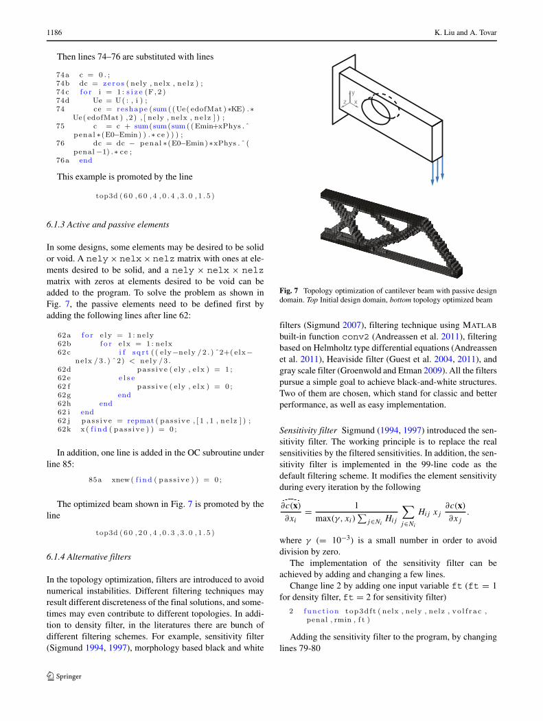
In some designs, some elements may be desired to be solidor void. A nely× nelx× nelz matrix with ones at ele-ments desired to be solid, and a nely × nelx × nelzmatrix with zeros at elements desired to be void can beadded to the program. To solve the problem as shown inFig. 7, the passive elements need to be defined first byadding the following lines after line 62:
In addition, one line is added in the OC subroutine underline 85:
The optimized beam shown in Fig. 7 is promoted by theline
6.1.4 Alternative filters
In the topology optimization, filters are introduced to avoidnumerical instabilities. Different filtering techniques mayresult different discreteness of the final solutions, and some-times may even contribute to different topologies. In addi-tion to density filter, in the literatures there are bunch ofdifferent filtering schemes. For example, sensitivity filter(Sigmund 1994, 1997), morphology based black and white
x
y
z
Fig. 7 Topology optimization of cantilever beam with passive designdomain. Top Initial design domain, bottom topology optimized beam
filters (Sigmund 2007), filtering technique using MATLAB
built-in function conv2 (Andreassen et al. 2011), filteringbased on Helmholtz type differential equations (Andreassenet al. 2011), Heaviside filter (Guest et al. 2004, 2011), andgray scale filter (Groenwold and Etman 2009). All the filterspursue a simple goal to achieve black-and-white structures.Two of them are chosen, which stand for classic and betterperformance, as well as easy implementation.
Sensitivity filter Sigmund (1994, 1997) introduced the sen-sitivity filter. The working principle is to replace the realsensitivities by the filtered sensitivities. In addition, the sen-sitivity filter is implemented in the 99-line code as thedefault filtering scheme. It modifies the element sensitivityduring every iteration by the following
�∂c(x)
∂xi
= 1
max(γ, xi)∑
j∈NiHij
∑
j∈Ni
Hij xj∂c(x)
∂xj
.
where γ (= 10−3) is a small number in order to avoiddivision by zero.
The implementation of the sensitivity filter can beachieved by adding and changing a few lines.
Change line 2 by adding one input variable ft (ft = 1for density filter, ft = 2 for sensitivity filter)
Adding the sensitivity filter to the program, by changinglines 79-80

An efficient 3D topology optimization code written in Matlab 1187
Changing the design variable update strategy (line 86) inthe optimal search procedure
Gray scale filter A simple non-linear gray-scale filter orintermediate density filter has been proposed by Groen-wold and Etman (2009) to further achieve black-and-whitetopologies. The implementation of the gray scale filter is bychanging the OC update scheme as the following
xnewi =
⎧⎨
⎩
max(0, xi − m), ifxiBηi � max(0, xi − m)
min(1, xi + m), ifxiBηi � min(1, xi − m)
(xiBηi )q, otherwise
(52)
The standard OC updating method is a special case of(52) with q = 1. A typical value of q for the SIMP-basedtopology optimization is q = 2.
The implementation of the gray scale filter to the codecan be done as follows:
Adding one input variable q to the program (line 2)
Change the OC updating method (line 85) to
The factor q should be increased gradually by adding oneline after line 68
Table 3 Time usage of finite element analysis time for differentsolvers
Mesh size Direct solver Iterative solver
30 × 10 × 2 0.018 sec 0.129 sec
60 × 20 × 4 0.325 sec 0.751 sec
150 × 50 × 10 74.474 sec 22.445 sec
Figure 8 demonstrates the optimized beams applying dif-ferent filtering techniques. As can be seen from final results,both sensitivity filter, density filter and gray scale filter sup-press checkerboard patterns. The gray scale filter combineswith the sensitivity filter provides the most black-and-whitesolution.
6.1.5 Iterative solver
If the finite element mesh size becomes large, the tra-ditional direct solver (line 72) used to address the finiteelement analysis is suffered by longer solving time andsome other issues. However, iterative solver (Hestenes andStiefel 1952; Augarde et al. 2006) can solve large-scaleproblems efficiently. To this end, line 72 is replaced bya built-in MATLAB function pcg, called preconditionedconjugate gradients method, as shown in the following
Direct solver is a special case by setting the precondi-tioner (line 72c) to
Table 3 gives the comparison of two different finite ele-ment analysis solvers. As shown in the table, a speed upfactor of 30.81 has been measured when solving large scaleproblem. Hence, the iterative solver is more suitable forlarge-scale problems, and vice versa.
Some examples include a cantilever beam, theMesserchimitt-Bolkow-Blohm (MBB) beam and L-shapeproblems (Table 4) are solved by using iterative solver
Fig. 8 Topology optimized design used a mesh with 30 × 10 × 2 ele-ments. Left optimized design using density filter, middle left optimizeddesign using density filter, middle right optimized design using density
filter and gray scale filter, and right optimized design using sensitivityfilter and gray scale filter

1188 K. Liu and A. Tovar
Table 4 Three-dimensionalexamples: Cantilever, MBB,and L-shape problem. Left:Initial design domains, right:topology optimized results
and applying gray scale filter. The underlined trianglerepresents a three-dimensional planar joint.
6.1.6 Continuation strategy
Convexity is a very preferable property since every localminima is also the global minima, and what the pro-gram is solving for is the global minima. Unfortunately,the use of SIMP method to achieve binary solution willdestroy the convexity of the optimization problem. For suchproblems, it is possible that for different starting pointsthe program converges to totally different local minima.In order to penalize intermediate densities and mitigatethe premature convergence to one of the multiple localminima when solving the non-convex problem, one could
perform a continuation step. As previously presented byGroenwold and Etman (2010), the continuation step is givenas
pk ={
1 k � 20,
min{pmax, 1.02pk−1} k > 20,(53)
where k is the iteration number, and pmax is the maximumpenalization power.
Though this methodology is not proven to converge tothe global optimum, it regularizes the algorithm and allowsthe comparison of different optimization strategies.
Implementing the continuation strategy is done by addinga single line after line 68:

An efficient 3D topology optimization code written in Matlab 1189
6.2 Compliant mechanism synthesis
A compliant mechanism problem involves loading cases:input loading case and dummy loading case. The codealso needs to implement a new objective function andits corresponding sensitivity analysis. To demonstrate thisimplementation, let us consider a three-dimensional forceinverter problem as shown in Fig. 9. With an input loaddefined in the positive direction, the design goal is to max-imize the negative horizontal output displacement. Boththe top face and the side force are imposed with sym-metric constraints; i.e., nodes can only move within theplane.
The new loading conditions as well as input and outputpoints are defined as follows:
and the boundary conditions are defined as below:
The external springs with stiffness 0.1 are added at inputand output points after line 71.
The expressions of the objective function (31) and sensi-tivity (32) are modified in lines 74-76.
x
yz
In
OutTop face constrained for symmetric
Side faceconstrainedfor symmetric
Fig. 9 Design domain of 3D force inverter problem
The convergence criteria for the bi-sectioning algorithm(lines 82-83) is improved by the following lines:
To improve the convergence stability, the damping factorof OC-method changes from 0.5 to 0.3 and also takes thepositive sensitivities into account, then line 85 is changed to:
The final design shown in Fig. 10 is promoted by the linein the MATLAB:
6.3 Heat conduction
The implementation of heat conduction problems is notmore complex than the one for compliant mechanism syn-thesis since the number of DOF per node is one rather
Fig. 10 Topology optimized force inverter
1190 K. Liu and A. Tovar
than three. Following the implementation of heat conduc-tion problems in two dimensions (Bendsøe and Sigmund2003), the implementation for three dimension problems issuggested in the following steps.
First, the elastic material properties (lines 8-10) arechanged to the thermal conductivities of materials
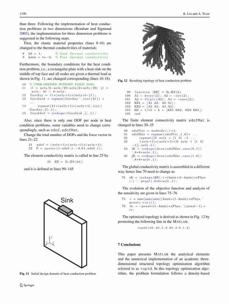
Furthermore, the boundary conditions for the heat condi-tion problem, i.e., a rectangular plate with a heat sink on themiddle of top face and all nodes are given a thermal load asshown in Fig. 11, are changed corresponding (lines 10-18).
Also, since there is only one DOF per node in heatcondition problems, some variables need to change corre-spondingly, such as ndof, edofMat.
Change the total number of DOFs and the force vector inlines 21–22
The element conductivity matrix is called in line 25 by
and it is defined in lines 99–145
Sink
x
y
z
Fig. 11 Initial design domain of heat conduction problem
Fig. 12 Resulting topology of heat conduction problem
The finite element connectivity matrix edofMat ischanged in lines 30–35
The global conductivity matrix is assembled in a differentway, hence line 70 need to change as
The evulation of the objective function and analysis ofthe sensitivity are given in lines 75–76
The optimized topology is derived as shown in Fig. 12 bypromoting the following line in the MATLAB:
7 Conclusions
This paper presents MATLAB the analytical elementsand the numerical implementation of an academic three-dimensional structural topology optimization algorithmreferred to as top3d. In this topology optimization algo-rithm, the problem formulation follows a density-based

An efficient 3D topology optimization code written in Matlab 1191
approach with a modified SIMP interpolation for physi-cal densities. The finite element formulation makes useof eight-node hexahedral elements for which a closed-form expression of the element stiffness matrix is derivedand numerically implemented. The hexahedral finite ele-ments are used to uniformly discretize a prismatic designdomain and solve three related topology optimizationproblems: minimum compliance, compliant mechanism,and heat conduction problems. For each problem, thispaper includes the analytical derivation of the sensitiv-ity coefficients used by three gradient-based optimiza-tion algorithms: SQP, MMA, and OC, which is imple-mented by default. For the implementation of SQP, thispaper derives an analytic expression for the second orderderivative.
The use of top3d is demonstrated through severalnumerical examples. These examples include problems witha variety of boundary conditions, multiple load cases, activeand passive elements, filters, and continuation strategiesto mitigate convergence to a local minimum. The archi-tecture of the code allows the user to map node coor-dinates of node degrees-of-freedom boundary conditions.In addition, the paper provides a strategy to handle largemodels with the use of an iterative solver. For large-scale finite-element models, the iterative solver is about30 times faster than the traditional direct solver. Whilethis implementation is limited to linear topology opti-mization problems with a linear constraint, it provides aclear perspective of the analytical and numerical effortinvolved in addressing three-dimensional structural topol-ogy optimization problems. Finally, additional academicresources such the use of MMA and SQP are available athttp://top3dapp.com.
Appendix A: Symbolic expression of k0
This appendix presents the analytical results of the elementstiffness matrix k0 as discussed in Section 3. This sym-bolic expression of k0 is also been used by the programsubroutine lk H8.
Recall that, for an eight-node hexahedral element, thestrain-displacement matrix B is defined by
B =
⎡
⎢⎢⎢⎢⎢⎢⎢⎢⎢⎢⎢⎢⎢⎣
∂n1(ξe)∂ξ1
0 0 · · · ∂nq(ξe)
∂ξ10 0
0 ∂n1(ξe)∂ξ2
0 · · · 0 ∂nq(ξe)
∂ξ2
0 0 ∂n1(ξe)∂ξ3
· · · 0 0∂nq(ξe)
∂ξ3
∂n1(ξe)∂ξ2
∂n1(ξe)∂ξ1
0 · · · ∂nq(ξe)
∂ξ2
∂nq(ξe)
∂ξ10
0 ∂n1(ξe)∂ξ3
∂n1(ξe)∂ξ2
· · · 0∂nq(ξe)
∂ξ3
∂nq(ξe)
∂ξ2
∂n1(ξe)∂ξ3
0 ∂n1(ξe)∂ξ1
· · · ∂nq(ξe)
∂ξ30 ∂nq(ξe)
∂ξ1
⎤
⎥⎥⎥⎥⎥⎥⎥⎥⎥⎥⎥⎥⎥⎦
,
for e = 1, . . . , 3 and q = 1, . . . , 8. The correspondingshape functions nq in a natural coordinate systems ξe aredefined by
nq(ξe) = 1
8
⎧⎪⎪⎪⎪⎪⎪⎪⎪⎪⎪⎪⎪⎪⎪⎨
⎪⎪⎪⎪⎪⎪⎪⎪⎪⎪⎪⎪⎪⎪⎩
(1 − ξ1)(1 − ξ2)(1 − ξ3)
(1 + ξ1)(1 − ξ2)(1 − ξ3)
(1 + ξ1)(1 + ξ2)(1 − ξ3)
(1 − ξ1)(1 + ξ2)(1 − ξ3)
(1 − ξ1)(1 − ξ2)(1 + ξ3)
(1 + ξ1)(1 − ξ2)(1 + ξ3)
(1 + ξ1)(1 + ξ2)(1 + ξ3)
(1 − ξ1)(1 + ξ2)(1 + ξ3)
⎫⎪⎪⎪⎪⎪⎪⎪⎪⎪⎪⎪⎪⎪⎪⎬
⎪⎪⎪⎪⎪⎪⎪⎪⎪⎪⎪⎪⎪⎪⎭
.
Substituting values to (11), the 24 × 24 element stiffnessmatrix k0
i for an eight-node hexahedral element can beexpressed as
k0i = 1
(ν + 1)(1 − 2ν)
⎡
⎢⎢⎣
k1 k2 k3 k4
kT2 k5 k6 kT
4kT
3 k6 kT5 kT
2k4 k3 k2 kT
1
⎤
⎥⎥⎦ ,
where
k1 =
⎡
⎢⎢⎢⎢⎢⎢⎣
k1 k2 k2 k3 k5 k5
k2 k1 k2 k4 k6 k7
k2 k2 k1 k4 k7 k6
k3 k4 k4 k1 k8 k8
k5 k6 k7 k8 k1 k2
k5 k7 k6 k8 k2 k1
⎤
⎥⎥⎥⎥⎥⎥⎦
,
k2 =
⎡
⎢⎢⎢⎢⎢⎢⎣
k9 k8 k12 k6 k4 k7
k8 k9 k12 k5 k3 k5
k10 k10 k13 k7 k4 k6
k6 k5 k11 k9 k2 k10
k4 k3 k5 k2 k9 k12
k11 k4 k6 k12 k10 k13
⎤
⎥⎥⎥⎥⎥⎥⎦
,
k3 =
⎡
⎢⎢⎢⎢⎢⎢⎣
k6 k7 k4 k9 k12 k8
k7 k6 k4 k10 k13 k10
k5 k5 k3 k8 k12 k9
k9 k10 k2 k6 k11 k5
k12 k13 k10 k11 k6 k4
k2 k12 k9 k4 k5 k3
⎤
⎥⎥⎥⎥⎥⎥⎦
,
k4 =
⎡
⎢⎢⎢⎢⎢⎢⎣
k14 k11 k11 k13 k10 k10
k11 k14 k11 k12 k9 k8
k11 k11 k14 k12 k8 k9
k13 k12 k12 k14 k7 k7
k10 k9 k8 k7 k14 k11
k10 k8 k9 k7 k11 k14
⎤
⎥⎥⎥⎥⎥⎥⎦
,
k5 =
⎡
⎢⎢⎢⎢⎢⎢⎣
k1 k2 k8 k3 k5 k4
k2 k1 k8 k4 k6 k11
k8 k8 k1 k5 k11 k6
k3 k4 k5 k1 k8 k2
k5 k6 k11 k8 k1 k8
k4 k11 k6 k2 k8 k1
⎤
⎥⎥⎥⎥⎥⎥⎦
,

1192 K. Liu and A. Tovar
k6 =
⎡
⎢⎢⎢⎢⎢⎢⎣
k14 k11 k7 k13 k10 k12
k11 k14 k7 k12 k9 k2
k7 k7 k14 k10 k2 k9
k13 k12 k10 k14 k7 k11
k10 k9 k2 k7 k14 k7
k12 k2 k9 k11 k7 k14
⎤
⎥⎥⎥⎥⎥⎥⎦
,
and
k1 = −(6ν − 4)/9,
k2 = 1/12,
k3 = −1/9,
k4 = −(4ν − 1)/12,
k5 = (4ν − 1)/12,
k6 = 1/18,
k7 = 1/24,
k8 = −1/12,
k9 = (6ν − 5)/36,
k10 = −(4ν − 1)/24,
k11 = −1/24,
k12 = (4ν − 1)/24,
k13 = (3ν − 1)/18,
k14 = (3ν − 2)/18.
As can be seen from above, the 64 × 64 entries in theelement stiffness matrix can be represented by fourteencomponents (but not independent!).
Appendix B: Derivation of the Hessian Matrix
In this appendix, we will discuss the derivation of the secondorder derivative of the objective function. Structure compli-ance will be used as the objective function, the expressionfor other objective functions can be derived similarly.
Recall that the first order derivative of the compliance isgiven by
∂c
∂ xi
= −uiT(
∂ki
∂ xi
)
ui ,
where by applying the modified SIMP method (6), we have
∂ki
∂ xi
= pxp−1i (E0 − Emin)k0
i . (B1)
Note that for brevity of notation, we omitted the depen-dence on x in this appendix.
A second differentiation of the compliance yields
∂2c
∂ xi ∂ xj
= ∂
∂ xj
[
−uiT ∂ki
∂ xi
ui
]
= − ∂uiT
∂ xj
(∂ki
∂ xi
)
ui − uiT(
∂ki
∂ xi ∂ xj
)
ui
− uiT(
∂ki
∂ xi
)∂ui
∂ xj
(B2)
From (B1), the middle term of (B2) goes to zero. In orderto get the expression for ∂ui/∂ xj in the first and third terms,let us rewriting (16) as
kiui = fi .
Now if we differentiate both sides with respect to xj , weget∂ki
∂ xj
ui + ki∂ui
∂ xj
= 0,
which yields∂ui
∂ xj
= −k−1i
(∂ki
∂ xj
)
ui . (B3)
Substitute (B3) into (B1), we have
∂2c
∂ xi ∂ xj
= −[
−k−1i
(∂ki
∂ xj
)
ui
]T∂ki
∂ xi
ui − uTi
∂ki
∂ xi
[
−k−1i
(∂ki
∂ xj
)
ui
]
,
= 2uTi
(∂ki
∂ xj
)
k−1i
(∂ki
∂ xi
)
ui ,
where the last equality holds since
uTi
(∂ki
∂ xj
)
k−1i
(∂ki
∂ xi
)
ui
={[
uTi
(∂ki
∂ xj
)
k−1i
] [(∂ki
∂ xi
)
ui
]}T
=[(
∂ki
∂ xi
)
ui
]T [
uTi
(∂ki
∂ xj
)
k−1i
]T
= uTi
(∂ki
∂ xi
)
k−1i
(∂ki
∂ xj
)
ui . (B4)
As discussed earlier, when i �= j , ∂ki /∂ xj = 0. When i = j ,subsituting (B1), (10) and (6) into (B4), we have
∂2c
∂ x2i
= 2 uTi
[pxp−1
i (E0 − Emin)k0i
][Emin+
xp
i (E0 − Emin)k0i
]−1 [pxp−1
i (E0 − Emin)k0i
]ui
= 2[pxp−1
i (E0 − Emin)]2 [
Emin + xp
i (E0 − Emin)]−1
uTi k0
i ui .
Therefore, the Hessian of the structural compliance isgiven by:
∂2c
∂ xi ∂ xj=
⎧⎪⎨
⎪⎩
0, i �= j,
2[pxp−1
i (E0 − Emin)]2 [
Emin + xpi (E0 − Emin)
]−1 uTi k0
i ui , i = j.
An efficient 3D topology optimization code written in Matlab 1193
Appendix C: MATLAB Program top3d
1194 K. Liu and A. Tovar
An efficient 3D topology optimization code written in Matlab 1195
References
Aage N, Nobel-Jørgensen M, Andreasen CS, Sigmund O (2013)Interactive topology optimization on hand-held devices. StructMultidiscip Optim 47(1):1–6
Allaire G (2001) Shape optimization by the homogenization method.Springer, New York
Allaire G, Kohn R (1993) Optimal design for minimum weight andcompliance in plane-stress using extremal microstructures. Eur JMech 12(6):839–878
Allaire G, Pantz O (2006) Structural optimization with freefem++.Struct Multidiscip Optim 32(3):173–181
Allaire G, Belhachmi Z, Jouve F (1996) The homogenization methodfor topology and shape optimization. single and multiple loadscase. Eur J Finite Elem 5:649–672
Allaire G, Jouve F, Toader AM (2004) Structural optimization usingsensitivity analysis and a level-set method. J Comput Phys194(1):363–393
Andreassen E, Clausen A, Schevenels M, Lazarov BS, Sigmund O(2011) Efficient topology optimization in matlab using 88 lines ofcode. Struct Multidiscip Optim 43(1):1–16
Augarde C, Ramage A, Staudacher J (2006) An element-based dis-placement preconditioner for linear elasticity problems. ComputStruct 84(31–32):2306–2315
Bendsøe MP (1989) Optimal shape design as a material distributionproblem. Struct Multidiscip Optim 1(4):193–202
Bendsøe MP (1995) Optimization of structural topology shape andmaterial. Springer, New York
Bendsøe MP, Kikuchi N (1988) Generating optimal topologies instructural design using a homogenization method. Comput Meth-ods Appl Mech Eng 71(2):197–224

1196 K. Liu and A. Tovar
Bendsøe MP, Sigmund O (2003) Topology optimization: theory,method and applications. Springer
Bruns TE, Tortorelli DA (2001) Topology optimization of non-linearelastic structures and compliant mechanisms. Comput MethodsAppl Mech Eng 190(26–27):3443–3459
Challis VJ (2010) A discrete level-set topology optimization codewritten in matlab. Struct Multidiscip Optim 41(3):453–464
Christensen PW, Klarbring A (2009) An introduction to structuraloptimization. Springer
Duysinx P (1997) Layout optimization: A mathematical program-ming approach, DCAMM report. Technical report, Danish Centerof Applied Mathematics and Mechanics, Technical University ofDenmark, DK-2800 Lyngby
Fleury C (1989) CONLIN: an efficient dual optimizer based on convexapproximation concepts. Struct Optim 1(2):81–89
Groenwold AA, Etman LFP (2009) A simple heuristic for gray-scalesuppression in optimality criterion-based topology optimization.Struct Multidiscip Optim 39(2):217–225
Groenwold AA, Etman LFP (2010) A quadratic approximation forstructural topology optimization. Int J Numer Methods Eng82(4):505–524
Guest JK, Prevost JH, Belytschko T (2004) Achieving minimumlength scale in topology optimization using nodal design vari-ables and projection functions. Int J Numer Methods Eng 61:238–254
Guest JK, Asadpoure A, Ha SH (2011) Elimiating beta-continuationfrom heaviside projection and density filter algorithms. StructMultidiscip Optim 44:443–453
Haber R, Jog C (1996) A new approach to variable-topology shapedesign using a constraint on perimeter. Struct Optim 11(1):1–12
Hassani B, Hinton E (1998) Homogenization and structural topologyoptimization: theory, practice and software. Springer
Hestenes MR, Stiefel E (1952) Methods of conjugate gradients forsolving linear systems. J Res Natl Bur Stand 49(6)
Hunter W (2009) Predominantly solid-void three-dimensional topol-ogy optimisation using open source software. Master’s thesis,University of Stellenbosch
Jog C (2002) Topology design of structures using a dual algorithmand a constraint on the perimeter. Int J Numer Methods Eng54(7):1007–1019
Kohn R, Strang G (1986a) Optimal design and relaxation of variationalproblems (part I). Commun Pure Applied Math 39(1):113–137
Kohn R, Strang G (1986b) Optimal design and relaxation of variationalproblems (part II). Commun Pure Appl Math 39(2):139–182
Kohn R, Strang G (1986c) Optimal design and relaxation of variationalproblems (part III). Commun Pure Appl Math 39(3):353–377
Liu Z, Korvink JG, Huang I (2005) Structure topology optimization:fully coupled level set method via FEMLAB. Struct MultidisciplOptim 6(29):407–417
Mlejnek H (1992) Some aspects of the genesis of structures. StructOptim 5(1–2):64–69
Nocedal J, Wright S (2006) Numerical optimization, 2nd edn. SpringerSchmit LA (1960) Structural design by systematic synthesis. In: 2nd
ASCE conference of electrical compounds. Pittsburgh, pp 139–149
Sigmund O (1994) Design of material structures using topologyoptimization, PhD thesis, Technical University of Denmark
Sigmund O (1997) On the design of compliant mechanisms usingtopology optimization. Mech Struct Mach 25(4):495–526
Sigmund O (2001) A 99 line topology optimization code written inmatlab. Struct Multidiscip Optim 21(2):120–127
Sigmund O (2007) Morphology-based black and white filters fortopology optimization. Struct Multidiscip Optim 33:401–424
Sigmund O, Peterson J (1998) Numerical instabilities in topologyoptimization: a survey on procedures dealing with checkerboards,mesh-dependencies and local minima. Struct Optim 16:68–75
Sokoł T (2011) A 99 line code for discretized michell truss optimiza-tion written in mathematica. Struct Multidiscip Optim 43(2):181–190
Suresh K (2010) A 199-line matlab code for pareto-optimal tracing intopology optimization. Struct Multidiscip Optim 42:665–679
Svanberg K (1987) The method of moving asymptotes-a new methodfor structural optimzation. Int J Numer Methods Eng 24:359–373
Talischi C, Paulino GH, Pereira A, Menezes IFM (2012a) Polymesher:a general-purpose mesh generator for polygonal elements writtenin matlab. Struct Multidiscip Optim 45:309–328
Talischi C, Paulino GH, Pereira A, Menezes IFM (2012b) Polytop: amatlab implementation of a general topology optimization frame-work using unstructured polygonal finite element meshes. StructMultidiscip Optim 45:329–357
Wang MY, Chen S, Xia Q (2004) Structural topology optimizationwith the level set method. http://www2.acae.cuhk.edu.hk/cmdl/download.htm
Wilson RB (1963) A simplicial method for convex programming, PhDthesis, Harvard University
Zhou M, Rozvany G (1991) The COC algorithm, part II: topological,geometrical and generalized shape optimization. Comp Meth ApplMech Eng 89:309–336
Zhou S, Wang MY (2005) 3d structural topology optimization with thesimp method. http://www2.acae.cuhk.edu.hk/cmdl/download.htm
![Efficient Reanalysis Procedures in Structural Topology Optimization1].pdf · In topology optimization, the nested approach is frequently applied, meaning optimization is performed](https://static.fdocuments.us/doc/165x107/5f43533d4fa1d652e3292cf2/efficient-reanalysis-procedures-in-structural-topology-optimization-1pdf-in.jpg)