EDUCATIONAL PAPER

A MATLAB code for topology optimization using the geometryprojection method

Hollis Smith1& Julián A. Norato1

Received: 19 December 2019 /Revised: 29 January 2020 /Accepted: 14 February 2020# The Author(s) 2020

AbstractThis work introduces a MATLAB code to perform the topology optimization of structures made of bars using the geometryprojection method. The primary objective of this code is to make available to the structural optimization community a simpleimplementation of the geometry projection method that illustrates the formulation and makes it possible to easily and efficientlyreproduce results. A guiding principle in writing the code is modularity, so that researchers can easily modify the program fortheir own purposes. Another goal is efficiency, for which extensive use of vectorization is made. This paper details the formu-lation of the geometry projection, discusses implementation aspects of the code, and demonstrates some of its capabilities bypresenting several 2D and 3D compliance minimization examples.

Keywords Topology optimization . Geometry projection

1 Introduction

The prevalent techniques to perform topology optimization ofcontinua are the density-based and the level-set methods(Sigmund andMaute 2013). These techniques produce organ-ic designs that are highly efficient. In some cases, a design thatclosely follows the optimal topology can be manufacturedusing, for example, additive manufacturing or casting tech-niques. However, when the most economical fabrication pro-cess consists of joining stock material such as bars or plates, itcan be very difficult to translate the optimal topology into adesign that conforms to that process. This difficulty has moti-vated the development of topology optimization techniquesthat produce designs exclusively made of geometricprimitives.

One of the topology optimization techniques that renderdesigns made of geometric components is the geometry

projection method (GPM) (Bell et al. 2012; Norato et al.2004, 2015). There exist other techniques to perform topologyoptimization using geometric components, such as the mov-ing morphable components method (Guo et al. 2014; Zhanget al. 2016b); a review of these techniques is outside of thescope of this paper; and we refer the reader to the recentreview by Wein et al. (2019). The purpose of this work is tointroduce a MATLAB code to illustrate the GPM for the to-pology optimization of 2D and 3D structures made of bars.The GPM is described in detail in Section 2. In particular, weaim to demonstrate how the geometry mapping can be per-formed in an efficient manner using vectorized operations.Unlike other educational codes published in this journal, wedo not attempt to fit the code into a relatively low number oflines and include it in the manuscript. Although this would bein principle possible, we believe in our case it would sacrificeclarity and therefore hinder the objective of explaining theinner workings of the geometry projection. Instead, this man-uscript provides an overview of the program, and the code isreleased for free and made available through GitHub at https://github.com/jnorato/GPTO. This approach allows us to bettermodularize the code but also to add various functionalities andoptions that users can experiment with, which we believe willbe beneficial to the research community. The code is releasedunder a Creative Commons CC-BY-NC 4.0 license, whichmeans it is free for non-commercial use and that appropriatecredit must be given. The program is not an open source

This work was supported by the U.S. Office of Naval Research, GrantNumber N00014-17-1-2505.

Responsible Editor: Xu Guo

* Julián A. Noratojulian.norato@uconn.edu

1 The University of Connecticut, 191 Auditorium Road, U-3139,Storrs, CT 06269, USA

Structural and Multidisciplinary Optimizationhttps://doi.org/10.1007/s00158-020-02552-0

program in the sense that a repository to which users cancontribute to further development of the code is not available.Nevertheless, the authors welcome any suggestions that usersmay have for future improvements.

The rest of the manuscript is structured as follows.Section 2 presents formulation of the geometry projectionmethod. In Section 3, details of the implementation are pro-vided. Some usage examples are presented in Section 4, andwe draw conclusions of this work in Section 5.

2 Geometry projection formulation

The basic idea of the geometry projection is to take a high-level parametric description of a geometric component ωb andmap it onto a pseudo-density field over a design region Ω ⊇ωb. This field is subsequently discretized via a fixed mesh foranalysis. The mapping must be differentiable so that designsensitivities of the optimization functions are well defined,and thus efficient gradient-based optimizers can be employed.This section describes the formulation of the geometry projec-tion and of the sensitivities.

2.1 Projected, penalized, and combined densities

We first consider the projection of a single geometric compo-nent. The projected density at a point x is the volume fractionof the intersection between the ball Br

x of radius r centered at xand the component ωb (Norato et al. 2004), i.e.,

ρ x; zb; rð Þ≔ jBrx∩ωb zbð ÞjjBr

xjð1Þ

where zb is the vector of geometric parameters that describeωb. For arbitrary shapes of the component ωb, computing ex-actly this intersection is not straightforward. Therefore, weseek an approximation of (1) that is easy to compute and isdifferentiable. If we assumeωb to be a smooth closedmanifoldand r to be sufficiently small, then ∂ωb∩Br

x can be approxi-mated as a line segment in 2D and a circle in 3D (since Br

x is acircle and a sphere, respectively). With that assumption, theprojected density can be approximated as the area fraction ofthe circular segment of height h = r − ϕb in 2D (or volumefraction of the spherical cap of the same height in 3D), whereϕb(x, zb) is the signed distance from x to ∂ωb (see Fig. 1).

1 Theprojected density is thus given by

ρbϕb x; zbð Þ

r

� �≔

0; if ϕb=r < −1eH ϕb=rð Þ; if−1≤ϕb=r≤11; if ϕb=r > 1;

8<: ð2Þ

where

eH xð Þ ¼1−

arccos xþ xffiffiffiffiffiffiffiffiffiffi1−x2

p

π; in 2D

1

2þ 3x

4−x3

4; in 3D:

8>><>>: ð3Þ

The notation eH is used here to bring attention to the factthat this is a regularized Heaviside; however, we emphasizethat it corresponds to the area (volume) fraction calculation ofthe circular (spherical) cap. The size r of the sample window isfixed throughout the optimization; hence, it is hereafter omit-ted as an argument. We also omit arguments on the right-handside of equations for brevity. The calculation of ϕb depends onthe particular representation of the geometric components. Inthe case of the offset bars considered in this work, it will bedetailed in Section 2.2.

A key ingredient of the geometry projection method is that,in addition to the parameters that describe the shape of eachcomponent, a size variable αb ∈ [0, 1] is ascribed to eachcomponent b. This size variable is penalized in the same spiritof penalization schemes employed in density-based topologyoptimization, so that a value of αb = 1 indicates the geometriccomponent must be part of the structure, while a value αb = 0indicates the component must be removed from the design.This feature makes it easier for the optimizer to remove geo-metric components and modify the topology. The penalizationis achieved via the definition of a penalized density bρb thatincorporates the size variable αb as

bρb x; zb; qð Þ≔μ αbρb; qð Þ; ð4Þ

Fig. 1 Geometry projection

1 Unlike previous works, here the signed distance is positive inside ωb andnegative outside, to be consistent with most of the literature.

H. Smith, J. A. Norato

where μ is a penalization function, q is the penalization pa-rameter, and we note that αb ∈ zb. For example, for a powerlaw penalization, as in the solid isotropic material penalization(SIMP) commonly used in density-based topology optimiza-tion, we have that μ(αbρb, q) = (αbρb)

q. Importantly, for thepenalization to be effective, it is required that the volume ofthe structure be computedwith the unpenalized density (e.g., q= 1 for SIMP).

Here we note that, unlike our previous works, the projecteddensity ρb is also penalized, as otherwise the material interpo-lation is linear in ρb when αb = 1, which renders a physicallyunrealistic material wherever intermediate-density materialappears (i.e., along the boundaries of geometric components),as demonstrated in Bendsøe and Sigmund (1999). We alsoobserve slightly better convergence with this modification,and this strategy produces less gaps in between componentsin the final design that are likely due to unrealistically stiffgray regions.

When multiple bars overlap, we combine the penalizeddensities for all bars into a combined density given by

ρ x; Z; pð Þ≔ρmin; if bρb ¼ 0; for b ¼ 1;⋯; nbgmax

bbρb

; otherwise;

8<: ð5Þ

where nb is the number of geometric components, gmax de-

notes a smooth approximation of the maximum function, Z≔

zT1 ;⋯; zTnb

h iTis the vector of design variables for all compo-

nents, and 0 < ρmin ≪ 1 is a positive lower bound to prevent anill-posed analysis. An example of a function that embodies (5)is the modified p-norm described in Zhang et al. (2016a):1

ρ x; Z; pð Þ≔ ρpmin þ 1−ρpmin

� �∑b¼1

nbbρpb� �1

p

: ð6Þ

This modified p norm renders ρ = ρmin, ifbρb ¼ 0∀b and ρ =1 if bρb ¼ 1∀b, regardless of the number of geometric compo-nents. Finally, the combined density is reflected in the analysisby using an ersatz material, with the elasticity tensor modifiedas

ℂ x; Zð Þ≔ρℂ0 ð7Þ

where ℂ0 is the elasticity tensor for the material the geometriccomponents are made of.

The foregoing formulation can be used for geometric com-ponents of any shape that are made of a single, isotropic ma-terial, so long as a signed distance and its derivatives withrespect to the geometric parameters can be computed. Forinstance, this scheme has been employed to design structuresmade of bars (Norato et al. 2015), flat plates (Zhang et al.

2016a), curved plates bent along a circular arc (Zhang et al.2018), and supershapes (Norato 2018), which are a generali-zation of hyperellipses with variable symmetry. The case ofmulti-material structures, where components can be made ofone out of a given set of isotropic materials, and where theoptimizer simultaneously determines the optimal componentslayout and the best material for each component, requires adifferent strategy to combine the geometric primitives and tointerpolate the properties of the different materials (cf. Wattsand Tortorelli (2017) and Kazemi et al. (2018)).

2.2 Distance

We now describe the computation of the signed distance ϕb in1. Here, as in some of our previous works, we represent barsas offset surfaces (Norato et al. 2015). Specifically, the bound-ary of the bar is given by the set of all points at a distance rb ofthe line segment with endpoints x1b and x2b (cf. Figure 1). Thisdefinition represents bars as rectangles with semicircular capsin 2D and cylinders with semispherical caps in 3D. The usermust define an initial design made of a set of bars; bars can beremoved from the design during the optimization (e.g., bysetting its size variable to zero) or reintroduced (by increasinga zero size variable), but in this code, bars cannot be intro-duced during the optimization.

The vector of design parameters for bar b in the offsetsurface representation is therefore given by zb = {x1b, x2b, rb,αb}. Our formulation allows for the case where endpoints areshared by two or more bars, thus they remain “connected” atthese endpoints throughout the optimization (much likeground structure approaches). The total number of design var-iables is 2(ndnp + nb), where nd = 2, 3 in 2D and 3D, respec-tively, and np is the total number of endpoints. Alternatively, abar can be defined to have its own medial axis endpoints, thusit can “float” within the design region independently of otherbars. If all bars are “floating,” then np = 2nb.

The advantage of using the offset surface representation isthat the signed distance to the boundary of the bar can simplybe computed as the distance to the medial axis (db) minus thebar radius as

ϕb x; zbð Þ ¼ db x; zbð Þ−rb: ð8Þ

To compute the distance to the bar’s boundary, it is there-fore only necessary to compute the distance to the bar’s medialaxis. Moreover, as we show in the sequel, the distance db andits design sensitivities can be computed in closed form as afunction of the bar’s design parameters zb.

Though not strictly necessary, an element-uniform combineddensity (5) is employed for the computation of the ersatz materialof (7). Therefore, the combined density and consequently thesigned distance are computed at the element centroid, whichwe denote as xe (cf. Figure 2). We also use the notation

A MATLAB code for topology optimization using the geometry projection method

xα=β≔xα−xβ: ð9Þ

The length of bar b is given by

ℓb ¼ ∥x2b=1b∥; ð10Þ

and the unit vector along the bar’s medial axis is given by

ab ¼x2b=1bℓb

: ð11Þ

Consider a Cartesian coordinate system for each bar inwhich x1b is the origin and ab is the first axis. On this coordi-nate system, ℓbe and rbe are, respectively, the parallel and per-pendicular components of xe/1b given by

ℓbe ¼ ab � xe=1b ð12Þrbe ¼ ∥rbe∥ ¼ ∥xe=1b−ℓbeab∥: ð13Þ

The distance from the medial segment of bar b to the cen-troid of element e is given by

dbe ¼∥xe=1b∥; if ℓbe≤0∥xe=2b∥; if ℓbe < ℓbrbe; otherwise

8<: ð14Þ

2.3 Optimization problem

The optimization problem solved by default in our code is thecompliance minimization problem given by

minZ

c u Zð Þð Þ≔∫Γtu Zð Þ � tdΓ ð15Þ

subject to

v f ≔1

jΩj ∫ΩρdΩ≤v*f ð16Þ

a u Zð Þ; vð Þ ¼ l vð Þ;∀v∈U0 ð17Þx1b; x2b∈Ω for b ¼ 1;⋯; nb ð18Þ

rbmin ≤rb≤rbmax ð19Þ0:0≤αb≤1:0; ð20Þwhere c is the compliance, vf is the volume fraction and v*f itslimit, and ρ is the combined density of (5). The domain Ωdenotes the region occupied by the design envelope, and Γt

and Γu denote the portions of ∂Ω where traction t and displace-ment boundary conditions u are imposed, respectively, with Γt ∪Γu = ∂Ω, Γt ∩ Γu = ∅ as usual. We assume there are no bodyloads and the applied traction is design-independent. The admis-sible sets for the trial displacement functions u and the test func-tions v are given by U≔ u u∈H1 Ωð Þ; u

Γ u¼ u

n oand

U0≔ v v∈H1 Ωð Þ; v Γ u

¼ 0n o

, respectively. The energy bilin-ear form a and the load linear form l in (17) are computed as

a u; vð Þ≔∫Ω∇Sv � ℂ∇SudΩ ð21Þwith ℂ the ersatz elasticity tensor of (7), ∇S the symmetric gra-dient operator and

l vð Þ≔∫Γt∇Sv � tdΓ: ð22Þ

2.4 Sensitivities

In this section, we present the expressions required to computeanalytical sensitivities of the compliance and volume fraction.For an optimization function θ that depends on the designexclusively and implicitly through the displacements, its sen-sitivity with respect to a design variable zi is given by

∂θ∂zi

¼ ∑e¼1

ne ∂θ∂ρe

∂ρe∂zi

; ð23Þ

where ne is the number of elements. Using adjoint analysis,and as customary in density-based topology optimization, forthe compliance (i.e., θ ≡ c) we have

∂c∂ρe

¼ −1

ρeue

TKeue ¼ −ue

TKe

0ue; ð24Þ

where ue is the vector of nodal displacements for element e,Ke

is the element stiffness matrix computed using the ersatz ma-terial of (7), and Ke

0 is the “fully solid” element stiffnes matrixcorresponding to ρe = 1. It should be noted that Ke

0 only needsto be computed once and for all in the optimization and storedin memory.

The sensitivity of the combined density, ∂ρe/∂zi in (23), isobtained from (5) as

∂ρe∂zi

¼ ∑b¼1

nb ∂ρe∂bρbe

∂bρbe∂zi

¼ ∑b¼1

nb ∂

∂bρbe gmaxb bρbe � ∂bρbe∂zi

; ð25Þ

where bρbe is the penalized density for element e and bar b of(4). It should be noted that ∂bρbe=∂zi is zero when zi does not

Fig. 2 Definition of vectors and quantities for distance computation

H. Smith, J. A. Norato

correspond to one of the design variables of bar b. The differ-ence between “floating” and “connected” bars is that in theformer case ∂bρbe=∂zi is non-zero for (at most) one bar and onlythe summand for the corresponding bar needs to be computed.The actual expression for the derivative of the smooth maxi-mum depends of course on the particular function chosen.

The sensitivities of the penalized density bρbe are obtainedfrom (4) as

∂bρbe∂zi

¼ ∂μ∂ αbρbeð Þ αb

∂ρbe∂zi

þ ρbe∂αb

∂zi

� �: ð26Þ

If zi corresponds to one of the components of x1b or x2b,then ∂αb/∂zi = 0 and the second term on the right-hand side of(26) vanishes. Conversely, if zi ≡αb, then ∂ρbe/∂zi = 0 and ∂αb/∂zi = 1, thus the first term on the right-hand side of (26)vanishes. Finally, if zi does not correspond to one of the designparameters of bar b, then the entire expression is zero.Consequently, each of the terms in the right-hand side of(26) is computed separately for each bar, and the sensitivitiesare subsequently “assembled” into a matrix.

From (2), the sensitivity of the projected density ρbe isgiven by

∂ρbe∂zi

¼1

r∂eH

∂ ϕbe=rð Þ∂ϕbe

∂ziif−1≤ϕbe=r≤1

0 otherwise:

8<: ð27Þ

This expression highlights the fact that the sensitivities ofthe projected density are non-zero only in a band of width 2ralong the bar boundary. From (3), we find

∂eH∂x

¼ 2ffiffiffiffiffiffiffiffiffiffi1−x2

p=π in 2D

3 1−x2� �

=4 in 3D;

�ð28Þ

with x = ϕbe/r. The sensitivities of the signed distance of (8)are given by

∂ϕbe

∂zi¼

∂dbe∂zi

if zi≡ x1bð Þk or x2bð Þk ; k ¼ 1;⋯; nd

−1 if zi≡rb0 otherwise;

8><>: ð29Þ

Finally, the sensitivities of the distance dbe with respect tothe bar endpoints xsb, s ∈ {1, 2} are given by

∂dbe∂xsb

¼ 1

dbe

−xe=1bδs1; if ℓbe≤0−xe=2bδs2; if ℓbe < ℓb

−rbe δs1 þℓbeℓb

δs2−δs1

� �� �otherwise;

8>><>>: ð30Þ

where δsk≔ 1 if s ¼ k; 0 otherwisef g is the Kronecker delta.It can be noted from (30) that ∂dbe/∂xsb is undefined when

dbe = 0 (Norato et al. 2015; Zhang et al. 2016a). In this case, an

element centroid xe lies exactly on the medial axis of bar b.This situation can be circumvented bymaking sure the samplewindow size is smaller than the bar’s width, i.e., r < rb, sincean infinitesimal perturbation of the bar’s medial axis endpointswill leave the projected density of any point on the medial axisunchanged (ρbe = 1), and thus ∂ρbe/∂xsb in (27) must necessar-ily be zero.

When the bar’s axis collapses to a point (so that ℓb = 0), thesensitivities are still well defined, since the first branch of (30)applies. However, since the code still computes ab/ℓb, wecheck ℓb against a small tolerance to prevent a division byzero.

The sensitivities of the volume fraction of (16) (i.e., θ ≡ vf)are computed as

∂v f∂zi

¼ 1

V∑e¼1

ne

ve∂ρe∂zi

; ð31Þ

where ve is the volume of element e and V ¼ ∑nee¼1ve is the

volume of the design region. The term ∂ρe/∂zi is computed asbefore using (25–30), however with the clarification that thevolume fraction must be computed with the unpenalized den-sity. Consequently, ∂μ/∂(αbρbe) = 1 in (26).

Most of the equation numbers for this section have beenadded to comments in the code so that the user can readily findthem (for instance, as shown in Appendix A).

2.5 Algorithm

We complete the presentation of the geometry projection for-mulation with the pseudo-code shown in Fig. 3. This algo-rithm presents a conceptual (but logically correct) flow of thesteps taken to perform the optimization. However, as will bementioned in the following section, an efficient implementa-tion of the code does not exactly follow this pseudo-code. InFig. 3,bz denotes the vector of design variables after they havebeen scaled so that they lie in the range [0, 1]. This scaling andthe imposition of move limits on each design update arediscussed in detail in Section 3.5.

3 Implementation

In this section, we discuss general aspects of the implementa-tion, particularly in terms of functionality of the code. We alsodiscuss in some detail the calculation of the geometry projec-tion described in the previous section. The code was devel-oped and tested using MATLAB, version R2018b. It was test-ed in the Red Hat Enterprise Linux 7.4, macOS Mojave, andWindows 10 operative systems. Because we make extensiveuse of vectorization, the code performs better in multi-coremachines. The code is executed by running the scriptGPTO.m (without any arguments). To check that the program

A MATLAB code for topology optimization using the geometry projection method

is running, we suggest the user simply runs this script, whichexecutes the optimization of a 2D cantilever beam (not de-scribed in this work).

It should be noted that performance will suffer drasticallyon non-Intel CPUs because Intel’s math kernel library (MKL)disables by default all but the most basic vectorization on non-Intel CPUs. However, this can be circumvented by setting anenvironment variable: MKL_DEBUG_CPU_TYPE = 5.

3.1 Organization

Since we do not attempt to write the code in as concise amanner as possible, we are free to modularize it as much aspossible, which we have attempted to do. Similar functions areplaced under the same subfolder—for instance, those relatedto the finite element analysis, geometry projection, optimiza-tion, plotting, etc. This allows the user to more easily navigatethe code, examine and focus on particular portions of theimplementation, and make changes. We have adhered to therule that one routine corresponds to one MATLAB script (i.e.,no script has multiple functions declared in it). The modularstructure also facilitates having multiple options for, e.g., thepenalization function μ of (4), the aggregation function of (5),the mesh input or generation, etc. The root folder only con-tains the main script GPTO.m and another script to invoke theinput functions (get_inputs.m); all other scripts are insidesubfolders.

Another important aspect of our implementation is that weuse three MATLAB structures, named FE, GEOM, and OPT,to store all information related to the finite element analysis,geometric components, and method parameters, respectively.

These structures are declared as global variables in any scriptwhere they are needed. Having only a few structures and de-claring them as global variables avoids having to pass longlists of arguments to the functions that need the informationstored in them. If a new field is added to one of these struc-tures, it becomes immediately available to any routine invok-ing the structure as a global variable. Using global variables isin general discouraged in modern compiled languages be-cause they may not be thread-safe; however, since we are onlyusing MATLAB’s own vectorized operations, we assume thatpotential problems such as race conditions are managed byMATLAB (and we have to date not observed any issue relatedto this in our numerical experiments). Also, the use of globalvariables makes the code slightly more efficient, since localcopies of the structures (some of which may be relativelylarge, such as FE) need not be created in each routine that usesthem.

3.2 Inputs

The user must provide all of the inputs usingMATLAB scripts.This strategy circumvents having to parse text files, allows inproviding inputs in any order, facilitates the incorporation ofcomments, and makes it easier for the user to customize thecode. Although not strictly necessary, we have placed all theinput files for the sample problems into the subfolder \texttt (infact, we created additional subfolders inside this subfolder foreach one of the examples). To switch from running one exam-ple to another, the user needs only to update the single line withthe run command in the inputs.m script located in the rootfolder to indicate the location of the master input file for therun. Having a script that calls the master input files makes iteasy to keep different inputs for different runs. Note that the\input_files subfolder is not added to the search path out ofprecaution to avoid potential name conflicts and because it isnot necessary for the code to run.

Since there are quite a few options in the program, theeasiest way to create input files for a new run is to copy andmodify the files for one of the sample problems. The inputfiles for all problems are well commented to make it easy tomodify them. All of the inputs are used to initialize the afore-mentioned three data structures that pertain to the finite ele-ment analysis, the bars that make up the initial design, and allparameters related to the geometry projection, the optimiza-tion problem, the optimizer, and the finite difference check ofsensitivities (if requested).

3.3 Finite element analysis

The parameters relating to the finite element mesh are placedin the FE.mesh_input structure. Three options are available tocreate or read a mesh, which are indicated in the type field.The ‘generate’ option creates a mesh on the fly for rectangular

Fig. 3 Algorithm for topology optimization using geometry projection

H. Smith, J. A. Norato

and cuboid design regions in 2D and 3D, respectively. Theuser must specify the dimensions of the region and the numberof elements along each dimension using the box_dimensionsand elements_per_side vectors, respectively. The second op-tion, ‘read-home-made’, can be used to read a mesh that hasbeen previously created (e.g., using the makemesh script pro-vided in the code) and saved to a MATLAB .mat file, whosepath must be provided in the field mesh_filename. The option‘read-gmsh’ allows the user to read a mesh created with theopen source software Gmsh (Geuzaine and Remacle 2009).The user must create a mesh made of quadrilateral orhexahedral elements in 2D or 3D, respectively (a transfinitemesh in Gmsh parlance); export it to MATLAB format; andindicate the path of this file in the gmsh_filename field. Thisthird option is very convenient for design regions that are notcuboid-shaped.

The mesh only contains the node locations and the elementconnectivity. Displacement boundary conditions and loadsmust be specified in a separate MATLAB script that the usermust create and whose path must be specified in the bcs_filefield. This separation facilitates using the same mesh for dif-ferent problems with different boundary conditions. As be-fore, it is easier to copy the file for one of the sample problemsand modi fy i t . For cubo id - shaped meshes , thecompute_predefined_node_sets function provides a very con-venient utility to retrieve node sets corresponding to pre-scribed points, edges, and faces of the domain, which can besubsequently used to impose displacement boundary condi-tions or to apply loads. These node sets are stored in theFE.node_set structure. For example, for a 2D rectangular do-main, the set BR_PT contains the node in the bottom-rightcorner of the domain, and the set L_edge contains all nodeson the left-hand side edge of the domain. Needless to say, theuser must ensure that the problem is sufficiently restrained toget a well-posed analysis.

The code for the finite element analysis closely follows thesparse data structures and vectorized operations presented inAndreassen et al. (2011). It provides the option to use a directo r a n i t e r a t i v e s o l v e r t h r ough t h e p a r ame t e rFE.analysis.solver.type. In the former case, we simply useMATLAB’s matrix left division operator “\”, which usesCholesky factorization. In the latter case, which may be usefulfor larger systems, we use the preconditioned conjugate gra-dient solver with an incomplete Cholesky preconditioner(using MATLAB’s pcg and ichol functions, respectively).For the iterative solver, the user must specify the convergencetolerance and the maximum number of iterations in the tol andmaxit fields, respectively.

The code also has an option to use a GPU card to solve thesystem of linear equations, by setting the parameterFE.analysis.solver.use_gpu to true, which can be used if thesystem has an NVIDIA GPU card. In this case, only the iter-ative solver can be used, and a Jacobi preconditioner is used

instead of the incomplete Cholesky preconditioner, sinceusing the latter incurs a high data transfer cost to the GPUmemory and is inefficient. The trade-off is that the iterativesolution requires more iterations with the Jacobipreconditioner; nevertheless, for large meshes, it is still fasterthan using the iterative solver with CPUs.

Table 1 shows the time it takes to perform one optimizationiteration using CPUs and GPUs in a system with an NVIDIAGTX 1070Max-Q GPU card and an Intel core i7 8750H (with6 cores) running on Ubuntu 19.10. The times correspond tothe average iteration time of the first two iterations for theoptimization of the default problem in the program (a 2Dcantilever beam with eight bars). These times thus includenot only the finite element analysis but also the geometryprojection and the design update by the optimizer. Althoughthe Jacobi preconditioner requires far more PCG iterations toconverge, it still outperforms the use of CPUs for these meshsizes (in this system). Also, it should be noted that the time andnumber of iterations will vary throughout the optimization,since different designs will lead to different condition numbersfor the system matrix. As the table shows, it can be veryconvenient to use GPUs in this code. For instance, a meshwith half a million elements requires about one and a halfminutes per iteration, therefore, 100 iterations of the optimi-zation can be completed in approximately two and a halfhours, which is—presently—very good for performing topol-ogy optimization in MATLAB on an individual workstation(recalling, however, that this is a 2D model).

3.4 Initial design

Through the GEOM.initial_design.path field in the master in-put file, the user must specify the path of the script containingthe specification of the bars that make up the initial design.This script contains two arrays that describe the initial layoutof bars. The point_matrix array has as many rows as points,with the first column containing an integer identifier for thepoint, and the remaining columns containing the spatial coor-dinates of the point. The bar_matrix array has as many rows as

Table 1 Averageoptimization iterationtimes for different sizemeshes of a 2D problem

Device Mesh size t (s) nPCG

cpu 320,000 61.6 1.2 k

gpu 320,000 71.9 6 k

cpu 500,000 115.2 1.5 k

gpu 500,000 90.2 7 k

cpu 749,088 198.4 1.8 k

gpu 749,088 152.9 8 k

cpu 999,698 301.7 2 k

gpu 999,698 223.2 9.5 k

nPCG is an approximate average number ofPCG iterations to convergence

A MATLAB code for topology optimization using the geometry projection method

bars. Its first column corresponds to an integer identifier forthe bar; the next two columns have the IDs of the points in thepoint_matrix array that correspond to the endpoints of thebar’s medial axis; and the fourth and fifth columns containthe initial values of the bar’s size variable and its radius,respectively.

It should be noted that this specification of points and barsallows for two possibilities: bars can be “floating” or “con-nected,” as detailed in Section 2.2. The computation of sensi-tivities (cf. (25)) in the code accounts for both situations.

As noted in Section 2.4, for sensitivities of the projecteddensity of (2) to be well defined, it is necessary that r < rb.Since we typically consider a sample window that at leastcovers each finite element, as detailed in Section 3.9, thisrequirement imposes a minimum element size. For example,if rbmin ¼ 1, and the sample window radius r is chosen to betwice the size of the element radius re, then re < 1/2 and

therefore the element size he should be at mostffiffiffi2

p=2 in 2D

andffiffiffi3

p=2 in 3D. To avoid undefined sensitivities in the initial

design, it is also necessary that the length of each bar is notzero, i.e., x1b ≠ x2b. Therefore, the user should not create initialdesigns with zero-length bars.

When running the optimization, the code saves the currentdesign (i.e., the arrays of points and bars) to aMATLAB .mat file.If the flag GEOM.initial_design.restart is set to true, the codereads the initial design from this file. This is a useful feature tostart an optimization from the design obtained by another opti-mization run or to perform a finite difference check of thesensitivities (as detailed in Section 3.7) on the final design ofa run. We note, however, that this does not constitute a cleancontinuation of a previous optimization run, since gradient-based optimizers (certainly the ones used in this code) useinformation from two or more consecutive iterations to con-struct approximations of the optimization functions.

3.5 Optimization

Although the code in its current form is written to solve theoptimization problem of (15)–(20), it is also structured so that(a) multiple constraints can be imposed and (b) any functioncan be chosen as the objective. This is achieved by indicatingin the master input file the name of the objective function(e.g., OPT.functions.objective = ‘compliance’;) and thenames and limits of the constraint functions (e.g.,OPT.functions.constraints={‘volume fraction’, ‘myconstraint’}; and OPT.functions.constraint_limit = [0.31.0];). In this example, the user has to implement the functionnamed ‘my constraint’ and add it to the list of available func-tions in the script init_optimization.m. This should facilitatethe modification of our code to address other optimizationproblems.

As opposed to density-based topology optimization, themagnitudes of the design variables in the geometry projectionscheme can differ greatly. Moreover, the optimization func-tions can be highly nonlinear with respect to the design vari-ables, and therefore the optimizer can take too large a designstep and produce poor iterates. To improve the performance ofthe optimization, we thus impose move limits on the designvariables. In order to impose the same relative move limit onall variables, we first scale the design variables as

zi ¼zi � zi�zi � zi�

; ð32Þ

where bzi is the scaled variable i and bzi and bzi are lower andupper bounds on the variables, respectively. For the compo-nents of the medial axis endpoints x1b and x2b, these boundsare given by the bounding box of the design region; for the barradius, they correspond to the values specified by the user inGEOM.min_bar_radius and GEOM.max_bar_radius; and thesize variables do not need any scaling. Variable scaling can beturned on or off using the parameter OPT.options.dv_scalingin the master input file. A move limit m is imposed on thedesign variables at iteration I as

max 0;bz I−1ð Þi −m

� �≤bz Ið Þ

i ≤min 1;bz I−1ð Þi þ m

� �: ð33Þ

The move limit value is assigned with the parametersOPT.options.move_limit in the master input file.

Two optimizers can be used with our code: MATLAB’sfmincon and the method of moving asymptotes (MMA)(Svanberg 1987, 2002, 2007). The choice of optimizer ismade with the parameter OPT.options.optimizer in the masterinput file. In the case of fmincon, we employ the active-set algorithm, since it allows us to impose move limits(through the ‘RelLineSrchBnd’ option as a relative bound onthe line search step length), and it performs well in our numer-ical experiments. fmincon handles well the situation where thelower bounds on a variable equal the upper bounds, and there-fore a fixed bar radius can be imposed if desired by settingGEOM.min_bar_radius = GEOM.max_bar_radius.

In addition to scaling the design variables, it is important toremember that in the case ofMMA, it is recommended that theconstraint limits and the objective function are between 1 and100 for reasonable values of the design variables. The volumefraction automatically satisfies this requirement, but the com-pliance does not. If the magnitude of the applied loading is toolarge and/or the elasticity modulus of the material is relativelylow, the compliance may easily exceed this range. The mini-mum compliance design for a given volume fraction does notdepend on the magnitude of the load or the elastic modulus.Therefore, the user can modify, for example, the load magni-tude to make sure the compliance is within the recommended

H. Smith, J. A. Norato

range. Another, more general strategy is to simply scale thecompliance and its sensitivities by some factor, which requiresmodifying the compute_compliance.m script accordingly.Ensuring proper scaling is important, as MMA may fail alto-gether if the magnitude of the compliance is very large.

In the case of MMA, we provide the code to call it in thescript runmma.m, but the user must obtain the MATLAB ver-sion of MMA from its author and copy the files mmasub.m,subsolv.m, and kktcheck.m in the optimization folder of ourcode. We employed the 2007 version of MMA (Svanberg(2007)) for numerical tests with our code. Unlike fmincon,MMA does not handle well the situation where the lowerand upper bounds of a variable are the same. Therefore, toapproximately impose a fixed bar radius, the user should setGEOM.max_bar_radius=GEOM.min_bar_radius+delta,where delta is a small positive number.

The code employs three stopping criteria. The first criterionis satisfied if the 2-norm of the change in the vector of designvariables falls below a specified value, indicated by the pa-rameter OPT.options.step_tol. The second is satisfied if thenorm of the Karush-Kuhn-Tucker optimality conditions fallsb e l ow t h e v a l u e s p e c i f i e d i n t h e p a r am e t e rOPT.options.kkt_tol. The third criterion is exceeding a maxi-mum number of iterations, given by the parameterOPT.options.max_iter. If any of these criteria are satisfied,the optimization is stopped.

3.6 Output

The program produces several forms of output. During thecourse of the optimization, two MATLAB figures are createdand updated at every iteration. The first is a plot of the barsdrawn by using directly the geometric parameters as rectan-gles with semicircular ends and colored such that the transpar-ency indicates the value of the size variable. A bar with a sizevariable value of unity has no transparency, and bars with asize variable value less than 0.05 are removed from the plot.

The second figure is a plot of the combined density of (5).In the case that fmincon is used as optimizer, this figure hastwo buttons to either pause or stop the optimization. At the endof the optimization, a third figure is produced that plots theiteration history of the objective and constraint functions. Thegeneration of these plots can be turned off by setting the var-iable plot_cond to false in the master input file; this option isconvenient when, for example, the code is executed in a queuein a high-performance computing system. The code alsowrites information on the optimization iterations toMATLAB’s Command Window.

Finally, our code writes Visualization Toolkit (.vtk) files ofthe combined density of the design to the folder specified inthe OPT.options.vtk_output_path parameter (which by defaultis set to ‘output_files’). The user can request VTK output fornone, all, or the last iteration by setting the parameter

OPT.options.write_to_vtk to ‘none’, ‘all’, or ‘last’, respective-ly. These files can be visualized with Open Source tools likeParaView (Ahrens et al. 2005; Ayachit 2015), which offerwide post-processing capabilities. This is particularly usefulfor 3D problems.

3.7 Finite difference check

Another utility provided by our code is a forward finite differ-ence check of the analytical sensitivities of the cost and/ orobjective functions. The finite difference check is turned on bysetting the parameter OPT.make_fd_check to ‘true’ in themaster input file. If this option is chosen, the code performsthe finite difference check and subsequently exits. The size ofthe finite difference step is specified in the parameterOPT.fd_step_size. The user can choose what function shouldbe checked by setting the parameters check_cost_sens andcheck_cons_sens to ‘true’ or ‘false’. This functionality is use-ful when developing new optimization functions to ensure theaccuracy of the analytical sensitivities.

3.8 Distance calculation

The computation of the distance dbe of (14) from the centroidxe of each element e to the medial axis of each bar b requires,conceptually, a double for loop, as shown in Fig. 3. This com-putation, which is of order O(nenb), can be quite expensive;however, it fortunately is embarrassingly parallel. In distribut-ed memory implementations, the elements in the mesh can bedivided among the available compute cores and each corecalculates the distance from those elements to all of the bars(see, e.g., Zhang et al. (2016a)). This computation scales lin-early with number of cores, and therefore if enough cores areemployed for the distance computation (as well as the calcu-lation of the combined density discussed in the following sec-tion), eventually the finite element analysis dominates the costof each function evaluation as the number of elements in-creases, and the geometry projection only represents a smallfraction of the cost.

When running on a single workstation with multiple cores,MATLAB employs shared-memory processing for many ofits vectorized operations. Therefore, as discussed inAndreassen et al. (2011), one of the keys to efficientimplementations of numerical methods in MATLAB is tovectorize the computations as much as possible. In particular,whenever a loop can be replaced with a vectorized operation,the improvements in performance can be drastic.

In the case of the distance calculation, the strategy we usedto vectorize the double for loop is to employ three-dimensional arrays, as can be seen in the excerpt of the dis-tance computation script shown in Appendix A. For instance,the array x_e_1b (line 36 in the code shown in the Appendix)contains all the vectors xe/1b, used in (12–14). The first

A MATLAB code for topology optimization using the geometry projection method

dimension of the array corresponds to the spatial componentsin the vector (of size 2 and 3 in 2D and 3D problems, respec-tively); the second dimension corresponds to the bar; and thelast to the element. Note that even the computation of thebranched function of 2 is vectorized by using Boolean matri-ces of dimensions 1 × nb × ne whose components equal true ifthe condition for the corresponding branch is satisfied andfalse otherwise (which are equivalent to 1 and 0, respectively).

As the problem size increases, accessing three-dimensionalmatrices can get quite slow (particularly if they have to bestored out of memory); therefore, eventually this approachbecomes inefficient. However, in our numerical experiments(and using our hardware), we have been able to run problemswith meshes that have hundreds of thousands of elements andtens of bars in reasonable times, and therefore this code shouldin many cases be efficient enough for method development(indeed, most publications with methods to perform topologyoptimization with geometric components use mesh sizes wellwithin this range).

Another important aspect of the code that is not explicitlystated in the pseudo-code of Fig. 3 is that the sensitivities ofeach quantity are computed in the same script where the quan-tity is computed, and they are then stored in the global struc-tures or passed to the calling function so that the chain rule isused for subsequent sensitivity calculations. For instance, thederivatives of the distance dbe in the script of Fig. 19 with

respect to the design parameters are computed in the samescript. This makes for a more modular code and makes iteasier to verify the correctness of the individual terms of thesensitivities. As with the distance calculation, the computationof the sensitivities makes extensive use of vectorization forefficiency.

3.9 Combined density calculation

The computation of the combined density of (5) is alsovectorized for efficiency. By default, the radius re of the sam-ple window in (2) is computed as the radius of the circle (in2D) or sphere (in 3D) that circumscribes the square or cubicelement, respectively, with the same volume of the element:

re ¼ffiffiffid

p

2veð Þ1d ð34Þ

where d = 2, 3 for 2D and 3D, respectively. This default can beoverridden by uncommenting the line with the parameterOPT.parameters.elem_r in the master input file and assigningto this parameter the actual value of the sample window radi-us. In this case, the same radius will be used for all elements inthe mesh.

The code has two options for the penalization function μ of(4), implemented in the script penalize.m: the SIMP penaliza-tion mentioned in Section 2.1 and the rational approximationof material properties (RAMP) (Stolpe and Svanberg 2001).The choice of penalization scheme is indicated by the param-eter OPT.parameters.penalization_scheme in the master inputfile, and the penalization parameter is assigned inOPT.parameters.penalization_param.

Several combination strategies are also available to com-pute the smooth maximum gmax of (5), implemented in thescript smooth_max.m. These include the modified p-norm of

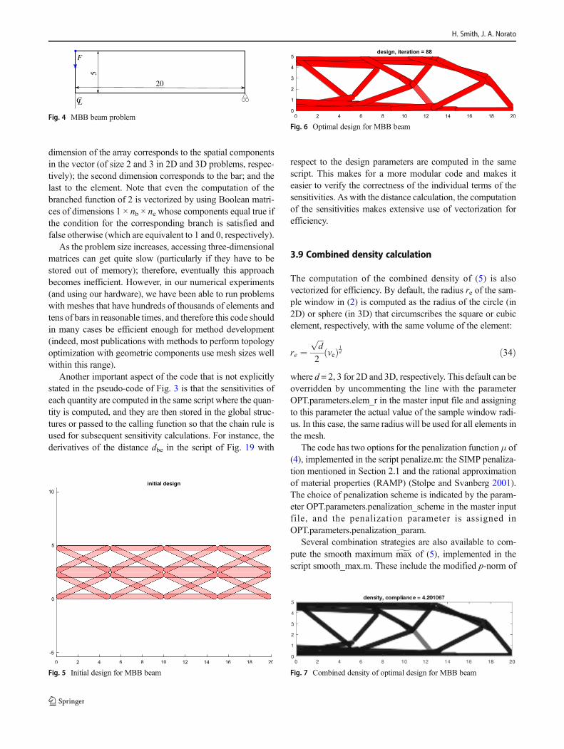
Fig. 5 Initial design for MBB beam

Fig. 6 Optimal design for MBB beamFig. 4 MBB beam problem

Fig. 7 Combined density of optimal design for MBB beam

H. Smith, J. A. Norato

(6), a modified p-mean, and lower- and upper-boundKreisselmeier-Steinhauser approximations. The choice ofcombination function is indicated in the parameterOPT.parameters.smooth_max_scheme, and the aggregationparameter (e.g., p in the p-norm) is assigned in the variableOPT.parameters.smooth_max_param. Once again, we havemade these functions modular so that the user can experimentwith different choices or implement their own.

4 Examples

In this section, we present several examples to demonstratesome capabilities of the program. The purpose of these exam-ples is not to demonstrate the geometry projection method but

the functionality of the code. The input files for all the exam-ples in this section are distributed with the code.

4.1 MBB beam

The first example corresponds to the widely studiedMesserschmitt-Bölkow-Blohm (MBB) beam. The dimen-sions, displacement boundary conditions (BCs), and load forthe MBB problem are shown in Fig. 4. The magnitude of theload is F = 0.1. The problem is symmetric with respect to thecenterline (only the right-hand side is shown in the figure).The volume fraction constraint for this problem is v*f ¼ 0:45.

0 10 20 30 40 50 60 70 80 90iteration

101

objective history

compliance

0 10 20 30 40 50 60 70 80 90iteration

0

0.2

0.4

0.6

0.8constraint history

volume fraction

Fig. 8 Optimization history ofcompliance and volume fractionfor MBB beam problem

Fig. 9 2D L-bracket problem

0 10 20 30 40 50 60 70 80 90 100

20

30

40

50

60

70

80

initial design

Fig. 10 Initial design for L-bracket

A MATLAB code for topology optimization using the geometry projection method

The reference manual that accompanies the code uses thisexample as a tutorial. It provides step-by-step instructions tocopy the input files of the default 2D cantilever problem andmodify them to solve the MBB design problem.

For this problem, we employ a mesh of square elements ofside 0.1. Bounds on the bars’ radii are imposed to enforce afixed bar radius rb = 0.25. The optimization is performedusing MMA. The initial design is made of 32 “floating” bars,shown in Fig. 5.

The optimal design, shown in Fig. 6, is obtained in 88iterations and in 80 s using a Mac Pro with a 3.5 GHz 6-Core Intel Xeon E5, running macOS Catalina 10.15.1, andMATLAB R2019b. The combined density of the optimal de-sign is shown in Fig. 7. The transparency of the bars in thisfigures indicates their size variable: a bar not shown (fullytransparent) has αb = 0, while a bar with no transparencyhas αb = 1. The initial design for this and all examples usesαb = 0.5 for all bars, and so the bars appear half transparent.The optimization history of the compliance (objective) andvolume fraction (constraint) is plotted in Fig. 8. All thesefigures are produced by the code.

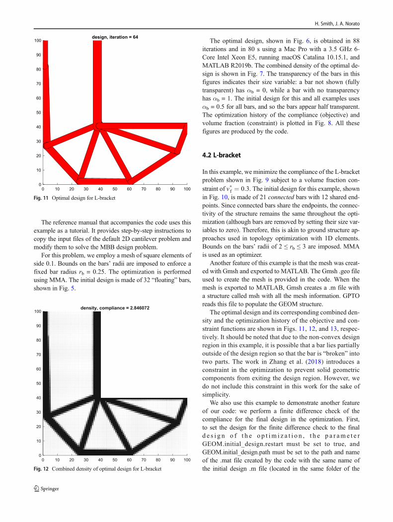
4.2 L-bracket

In this example, we minimize the compliance of the L-bracketproblem shown in Fig. 9 subject to a volume fraction con-straint of v*f ¼ 0:3. The initial design for this example, shownin Fig. 10, is made of 21 connected bars with 12 shared end-points. Since connected bars share the endpoints, the connec-tivity of the structure remains the same throughout the opti-mization (although bars are removed by setting their size var-iables to zero). Therefore, this is akin to ground structure ap-proaches used in topology optimization with 1D elements.Bounds on the bars’ radii of 2 ≤ rb ≤ 3 are imposed. MMAis used as an optimizer.

Another feature of this example is that the mesh was creat-ed with Gmsh and exported to MATLAB. The Gmsh .geo fileused to create the mesh is provided in the code. When themesh is exported to MATLAB, Gmsh creates a .m file witha structure called msh with all the mesh information. GPTOreads this file to populate the GEOM structure.

The optimal design and its corresponding combined den-sity and the optimization history of the objective and con-straint functions are shown in Figs. 11, 12, and 13, respec-tively. It should be noted that due to the non-convex designregion in this example, it is possible that a bar lies partiallyoutside of the design region so that the bar is “broken” intotwo parts. The work in Zhang et al. (2018) introduces aconstraint in the optimization to prevent solid geometriccomponents from exiting the design region. However, wedo not include this constraint in this work for the sake ofsimplicity.

We also use this example to demonstrate another featureof our code: we perform a finite difference check of thecompliance for the final design in the optimization. First,to set the design for the finite difference check to the finald e s i g n o f t h e o p t i m i z a t i o n , t h e p a r am e t e rGEOM.initial_design.restart must be set to true, andGEOM.initial_design.path must be set to the path and nameof the .mat file created by the code with the same name ofthe initial design .m file (located in the same folder of the

0 10 20 30 40 50 60 70 80 90 1000

10

20

30

40

50

60

70

80

90

100design, iteration = 64

Fig. 11 Optimal design for L-bracket

0 10 20 30 40 50 60 70 80 90 1000

10

20

30

40

50

60

70

80

90

100density, compliance = 2.846072

Fig. 12 Combined density of optimal design for L-bracket

H. Smith, J. A. Norato

ma s t e r i n p u t f i l e ) . S e c o n d , t h e p a r am e t e r sOPT.make_fd_check and OPT.check_cost_sens must be setto true. The perturbation size for the finite difference checkis set as OPT.fd_step_size=1e-6;.

The largest absolute and relative differences between theanalytical sensitivities and the finite difference sensitivities arereported toMATLAB’s CommandWindow as − 0.0037 and −0.0013, respectively, indicating a good agreement. They cor-respond to the x component of the eighth point, which is thepoint closest to the right-hand side corner of the top edge. Thecode also produces a plot comparing the two sensitivities,shown in Fig. 14.

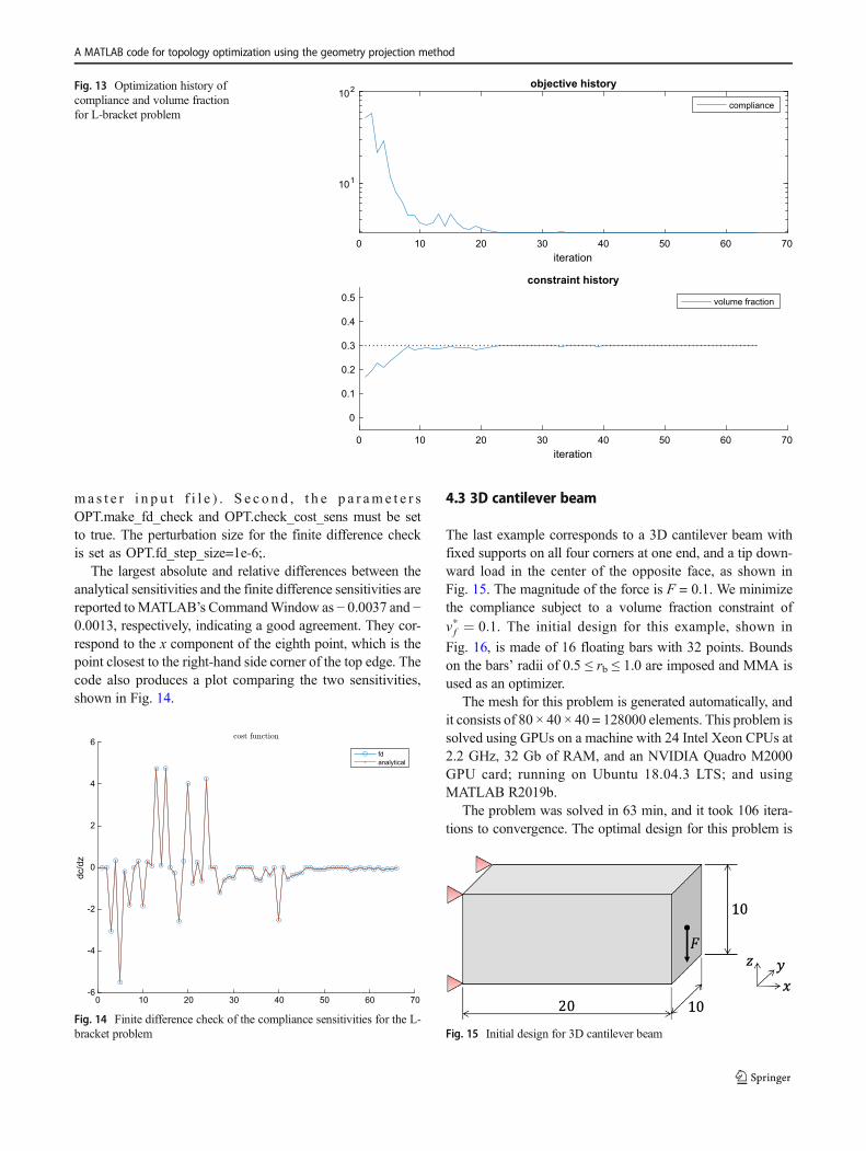
4.3 3D cantilever beam

The last example corresponds to a 3D cantilever beam withfixed supports on all four corners at one end, and a tip down-ward load in the center of the opposite face, as shown inFig. 15. The magnitude of the force is F = 0.1. We minimizethe compliance subject to a volume fraction constraint ofv*f ¼ 0:1. The initial design for this example, shown in

Fig. 16, is made of 16 floating bars with 32 points. Boundson the bars’ radii of 0.5 ≤ rb ≤ 1.0 are imposed and MMA isused as an optimizer.

The mesh for this problem is generated automatically, andit consists of 80 × 40 × 40 = 128000 elements. This problem issolved using GPUs on a machine with 24 Intel Xeon CPUs at2.2 GHz, 32 Gb of RAM, and an NVIDIA Quadro M2000GPU card; running on Ubuntu 18.04.3 LTS; and usingMATLAB R2019b.

The problem was solved in 63 min, and it took 106 itera-tions to convergence. The optimal design for this problem is

0 10 20 30 40 50 60 70iteration

101

102 objective history

compliance

0 10 20 30 40 50 60 70iteration

0

0.1

0.2

0.3

0.4

0.5

constraint history

volume fraction

Fig. 13 Optimization history ofcompliance and volume fractionfor L-bracket problem

0 10 20 30 40 50 60 70-6

-4

-2

0

2

4

6

dc/d

z

fdanalytical

Fig. 14 Finite difference check of the compliance sensitivities for the L-bracket problem Fig. 15 Initial design for 3D cantilever beam

A MATLAB code for topology optimization using the geometry projection method

shown in Fig. 17. An isosurface plot of the combined densityfor the optimal design (ρ = 0.5) produced using ParaView isshown in Fig. 18. This figure is produced by opening the filedens106.vtk file created by the code and saved to the/output_files folder, subsequently applying the following fil-ters in this order: Clean to Grid; Cell Data to Point Data; Cleanto Grid; Clip, changing the type to scalar and setting the valueto 0.5; Extract Surface; and Generate Surface Normal.

5 Conclusions

This paper presents a MATLAB code to perform topologyoptimization of 2D and 3D structures made of cylindrical barsby using geometry projection. The formulation of the method

is presented in full along with implementation details to aidusers in understanding and using the code. The program iswritten in a modular manner to facilitate modification andexperimentation. Vectorization is used extensively to renderan efficient code. The presented examples demonstrate someof the most important features of the code. The program isaccompanied by a reference manual with a step-by-step tuto-rial to reproduce the first example in this paper. The authorshope this is a useful contribution to the community and wel-come comments on this code.

Acknowledgments The authors express their gratitude to Prof. KristerSvanberg for providing his MMA MATLAB optimizer to perform theoptimization.

Funding information The authors express their gratitude to the USOfficeof Naval Research (Grant Number N00014-17-1-2505) for the support toconduct this work.

Compliance with ethical standards

Conflict of interests statement The authors declare that they have noconflict of interest.

Replication of results All the results presented in this work can bereproduced with the MATLAB code available from GitHub.

Appendix: code for distance calculation

F i g u r e 1 9 s h o w s t h e f i r s t p a r t o f t h ecompute_bar_elem_distance.m script that computes the dis-tance between the centroid of every element in the mesh tothe medial axis of each of the bars. The latter portion of thecode, which computes the derivatives of the distance withrespect to the medial axes endpoint x1b and x2b is omitted forbrevity.

Fig. 16 Initial design for 3D cantilever beam

Fig. 17 Optimal design for 3D cantilever beam

Fig. 18 Combined density isosurface for optimal design of 3D cantileverbeam

H. Smith, J. A. Norato

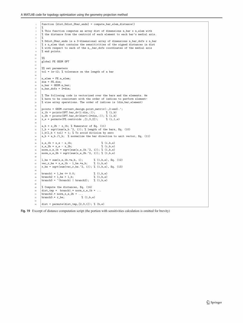
Fig. 19 Excerpt of distance computation script (the portion with sensitivities calculation is omitted for brevity)

A MATLAB code for topology optimization using the geometry projection method

Open Access This article is licensed under a Creative CommonsAttribution 4.0 International License, which permits use, sharing,adaptation, distribution and reproduction in any medium or format, aslong as you give appropriate credit to the original author(s) and thesource, provide a link to the Creative Commons licence, and indicate ifchanges weremade. The images or other third party material in this articleare included in the article's Creative Commons licence, unless indicatedotherwise in a credit line to the material. If material is not included in thearticle's Creative Commons licence and your intended use is notpermitted by statutory regulation or exceeds the permitted use, you willneed to obtain permission directly from the copyright holder. To view acopy of this licence, visit http://creativecommons.org/licenses/by/4.0/.

References

Ahrens J, Geveci B, Law C (2005) Paraview: an end-user tool for largedata visualization. The visualization handbook 717

Andreassen E, Clausen A, Schevenels M, Lazarov BS, Sigmund O(2011) Efficient topology optimization in matlab using 88 lines ofcode. Struct Multidiscip Optim 43(1):1–16

Ayachit U (2015) The Paraview guide: a parallel visualization applica-tion. Kitware, Inc.

Bell B, Norato J, Tortorelli D (2012) A geometry projection method forcontinuum-based topology optimization of structures. In: 12thAIAA Aviation Technology, Integration, and Operations (ATIO)Conference and 14th AIAA/ISSMO Multidisciplinary Analysisand Optimization Conference

Bendsøe MP, Sigmund O (1999) Material interpolation schemes in topol-ogy optimization. Arch Appl Mech 69(9–10):635–654

Geuzaine C, Remacle JF (2009) Gmsh: a 3-d finite element mesh gener-ator with built-in pre-and post-processing facilities. Int J NumerMethods Eng 79(11):1309–1331

Guo X, Zhang W, Zhong W (2014) Doing topology optimization explic-itly and geometrically—a new moving morphable componentsbased framework. J Appl Mech 81(8)

Kazemi H, Vaziri A, Norato JA (2018) Topology optimization of struc-tures made of discrete geometric components with different mate-rials. J Mech Des 140(11):111,401

Norato J, Haber R, Tortorelli D, Bendsøe MP (2004) A geometry projec-tion method for shape optimization. Int J Numer Methods Eng60(14):2289–2312

Norato J, Bell B, Tortorelli D (2015) A geometry projection method forcontinuum-based topology optimization with discrete elements.Comput Methods Appl Mech Eng 293:306–327

Norato JA (2018) Topology optimization with supershapes. StructMultidiscip Optim 58(2):415–434

Sigmund O, Maute K (2013) Topology optimization approaches. StructMultidiscip Optim 48(6):1031–1055

Stolpe M, Svanberg K (2001) An alternative interpolation scheme forminimum compliance topology optimization. Struct MultidiscipOptim 22(2):116–124

Svanberg K (1987) The method of moving asymptotes—a new methodfor structural optimization. Int J Numer Methods Eng 24(2):359–373

Svanberg K (2002) A class of globally convergent optimization methodsbased on conservative convex separable approximations. SIAM JOptim 12(2):555–573

Svanberg K (2007) MMA and GCMMA, versions september 2007.Optim Syst Theory 104

Watts S, Tortorelli DA (2017) A geometric projection method for design-ing three-dimensional open lattices with inverse homogenization. IntJ Numer Methods Eng 112(11):1564–1588

Wein F, Dunning P, Norato JA (2019) A review on feature-mappingmethods for structural optimization. arXiv 1910.10770

Zhang S, Norato JA, Gain AL, Lyu N (2016a) A geometry projectionmethod for the topology optimization of plate structures. StructMultidiscip Optim 54(5):1173–1190

Zhang S, Gain AL, Norato JA (2018) A geometry projection method forthe topology optimization of curved plate structures with placementbounds. Int J Numer Methods Eng 114(2):128–146

Zhang W, Yuan J, Zhang J, Guo X (2016b) A new topology optimizationapproach based on moving morphable components (MMC) and theersatz material model. Struct Multidiscip Optim 53(6):1243–1260

Publisher’s note Springer Nature remains neutral with regard to juris-dictional claims in published maps and institutional affiliations.

H. Smith, J. A. Norato