An Analytical Tool for Calculating Co-Channel Interference ......system interference, mainly...

An Analytical Tool for Calculating Co-Channel Interference in Satellite Links That Utilize Frequency

Reuse

Saurbh Chhabra

Thesis submitted to the faculty of the Virginia Polytechnic Institute and State University in partial fulfillment of the requirements for the degree of

Master of Science

In Electrical Engineering

Dr. Amir I. Zaghloul, Chair Dr. Gary Brown Dr. Ozlem Kilic

Dr. Timothy Pratt

September 8, 2006 Arlington, VA

Keywords: Co-Channel Interference, Satellite-based cellular network, Frequency Reuse, Carrier to Interference ratio (CIR), Carrier to Noise ratio (CNR), Carrier to Noise plus

Interference ratio (CNIR)

Copyright 2006, Saurbh Chhabra

An Analytical Tool for Calculating Co-Channel Interference in Satellite

Links That Utilize Frequency Reuse

Saurbh Chhabra

Abstract

This thesis presents the results of the development of a user-friendly computer

code (in MATLAB) that can be used to calculate co-channel interferences, both in the

downlink and in the uplink of a single satellite/space-based mobile communications

system, due to the reuse of frequencies in spot beams or coverage cells. The analysis and

computer code can be applied to any type of satellite or platform elevated at any height

above earth. The cells or beams are defined in the angular domain, as measured from the

satellite or the elevated platform, and cell centers are arranged in a hexagonal lattice. The

calculation is only for a given instant of time for which the system parameters are input

into the program.

The results obtained in one program run are for the overall carrier to interference

ratio (CIR) along with CIR for both the uplink and downlink paths. An overall carrier to

noise plus interference ratio (CNIR) is also calculated, which exemplifies the degradation

in the carrier to noise ratio (CNR) of the system.

Comparisons for systems with differing system scenarios are also made. For

example, overall CIRs are compared for different reuse numbers (3, 4, 7, and 13) in LEO

and GEO satellite systems.

In conclusion, as expected, it is observed that the co-channel interference

generally increases as we decrease the reuse number employed for the frequency reuse in

the cells. It is also observed that co-channel interference can cause substantial

degradation to the overall CNR of a system.

iii

Acknowledgments

I wish to express my deepest gratitude to everyone who has motivated me and/or

supported me for the completion of this work and especially to Dr. Amir Zaghloul for his

precious time, constant support and indulgence in this work. I would also like to thank

Dr. Ozlem Kilic for her time and expert advice in the course of this thesis work.

Special thanks to my wife, my daughter, my parents, sister, brother-in-law, others

in the family and friends for supporting me in this pursuit.

iv

Table of Contents

Abstract.............................................................................................................................. ii

Acknowledgments ............................................................................................................ iii

Table of Contents ............................................................................................................. iv

List of Figures................................................................................................................... vi

List of Tables ................................................................................................................... vii

Glossary .......................................................................................................................... viii

CHAPTER 1: Introduction.............................................................................................. 1

1.1 Motivation.................................................................................................................... 1

CHAPTER 2: Code Development ................................................................................... 4

2.1 Methodology ................................................................................................................ 4

2.2 Assumptions................................................................................................................. 6

2.3 Flowchart ..................................................................................................................... 7

2.4 Input File for the Program....................................................................................... 10

2.5 Calculation of Uplink Co-Channel Interference.................................................... 15

2.6 Calculation of Downlink Co-Channel Interference ............................................... 23

CHAPTER 3: LEO Interference Case with Reuse Numbers 3, 4, and 7................... 24

3.1 Overview .................................................................................................................... 24

3.2 Program Run Results ............................................................................................... 25

CHAPTER 4: GEO Interference Case with Reuse Numbers 3, 7, and 13 ................ 31

4.1 Overview .................................................................................................................... 31

4.2 Program Run Results ............................................................................................... 32

CHAPTER 5: Conclusions, Limitations and Future Work........................................ 38

5.1 Conclusions................................................................................................................ 38

5.2 Limitations and Future Work.................................................................................. 39

References ........................................................................................................................ 40

Appendix A: Program Flow for the Computer Code.................................................. 41

Appendix B: Main Computer Code .............................................................................. 44

Appendix C: User-Defined Functions Called by the Main Computer Code............. 68

Appendix D: Verification of the CNR Calculation ...................................................... 89

D.1 Sample Input for the Main Computer Code ......................................................... 89

v

D.2 Resulting Plots for the Sample Input ..................................................................... 91

D.3 Numerical Results for the Sample Input ............................................................... 94

Appendix E: Verification of the CIR Calculation........................................................ 97

E.1 Sample Input for the Main Computer Code.......................................................... 97

E.2 Resulting Plots for the Sample Input...................................................................... 99

E.3 Numerical Results for the Sample Input.............................................................. 101

E.4 Hand Calculations.................................................................................................. 103

Vita ................................................................................................................................. 106

vi

List of Figures

Figure 1.1. Depiction of the Satellite Uplink and Downlink Co-channel Interferers ........ 2

Figure 2.1. Program Flowchart for the Calculation of Overall CNR and CNIR…………9

Figure 2.2. Earth and Satellite Geometry used to test for Satellite Visibility.................. 11

Figure 2.3. 2-D Cross-section of Circularly Symmetric Antenna Patterns for Different

Taper Values .................................................................................................. 15

Figure 2.4. An Example of Hexagonal Tessellation in the Angular Domain for Nreuse= 7

....................................................................................................................... 17

Figure 2.5. Earth and Satellite Centric Coordinate Systems............................................ 20

Figure 3.1. LEO: Angular Distribution of Co-channel Beam Centers for the UPLINK &

DOWNLINK for Reuse # 3........................................................................... 28

Figure 3.2. LEO: Normalized Antenna Pattern of the UPLINK & DOWNLINK Satellite

Antennas for a Uniform Illumination ............................................................ 29

Figure 4.1. GEO: Angular Distribution of Co-channel Beam Centers for the UPLINK &

DOWNLINK for Reuse # 7........................................................................... 35

Figure 4.2. GEO: Normalized Antenna Pattern of the UPLINK & DOWNLINK Satellite

Antennas for a Uniform Illumination ............................................................ 36

Figure D1. Normalized Antenna Pattern of the UPLINK Satellite Antenna Along With

Angles for the Interferers............................................................................... 92

Figure D2. Distribution of Co-channel Beam Centers for the UPLINK Along With

Angular Locations of the Interferers.............................................................. 93

Figure D3. Distribution of Co-channel Beam Centers for the DOWNLINK Along With

Angular Locations of the Interferers.............................................................. 94

Figure E1. Normalized Antenna Pattern of the UPLINK/DOWNLINK Satellite Antennas

Along With Angles for the Interferers......................................................... 100

Figure E2. Distribution of Co-channel Beam Centers for the UPLINK/DOWNLINK

Along With Angular Locations of the Interferers........................................ 101

vii

List of Tables

Table 2.1. General Parameters and Their Sample Values from the Input Excel File ...... 10

Table 2.2. Uplink Parameters and Their Sample Values from the Input Excel File........ 12

Table 2.3. Downlink Parameters and Their Sample Values from the Input Excel File ... 13

Table 2.4. Sidelobe Levels for Different Taper Values ................................................... 14

Table 3.1. Parameters and Values Used for a LEO Scenario........................................... 24

Table 3.2. LEO: Lat/Long for the Sub-Satellite Point and Center of Coverage .............. 25

Table 3.3. LEO: General Parameters and Their Sample Values ...................................... 25

Table 3.4. LEO: Uplink Parameters and Their Sample Values ....................................... 26

Table 3.5. LEO: Downlink Parameters and Their Sample Values................................... 27

Table 3.6. LEO: Worst Case, Best Case, and Random case CNIR values ...................... 30

Table 3.7. LEO: Sample Runs of the Program for the Random Case only...................... 30

Table 4.1. Parameters and Values Used for a GEO Scenario .......................................... 31

Table 4.2. GEO: Lat/Long for the Sub-Satellite Point and Center of Coverage.............. 32

Table 4.3. GEO: General Parameters and Their Sample Values ..................................... 33

Table 4.4. GEO: Uplink Parameters and Their Sample Values ....................................... 33

Table 4.5. GEO: Downlink Parameters and Their Sample Values .................................. 34

Table 4.6. GEO: Worst Case, Best Case, and Random case CNIR values ...................... 37

Table 4.7. GEO: Sample Runs of the Program for the Random Case only ..................... 37

Table D1. General Parameters and Their Sample Values from the Input Excel File ...... 89

Table D2. Uplink Parameters and Their Sample Values from the Input Excel File ........ 90

Table D3. Downlink Parameters and Their Sample Values from the Input Excel File ... 91

Table E1. General Parameters and Their Sample Values from the Input Excel File....... 97

Table E2. Uplink Parameters and Their Sample Values from the Input Excel File ........ 98

Table E3. Downlink Parameters and Their Sample Values from the Input Excel File ... 99

viii

Glossary θ3dB 3-dB Beamwidth (usually in degrees) BER Bit Error Ratio BW Bandwidth (usually in MHz) CDMA Code Division Multiple Access CIR Carrier to Interference Ratio (usually in dB) CNR Carrier to Noise Ratio (usually in dB) CNIR Carrier to Noise plus Interference Ratio (usually in dB) DL Satellite Downlink ES Earth Station FDMA Frequency Division Multiple Access FEC Forward Error Correction GEO Geosynchronous or Geostationary Earth Orbit GTX, GRX Gain of the Transmitter’s or Receiver’s Antenna (usually in dBi) LEO Low Earth Orbit Lpath Free Space Path Loss (usually in dB) Lscan Antenna Scan Loss (usually in dB) Latm Clear Sky Atmospheric Loss (usually in dB) Lmisc Any Miscellaneous Losses (usually in dB) MEO Medium Earth Orbit MT Mobile Terminal Nreuse Reuse Number OBP On-Board Processing SNR Signal to Noise Ratio (usually in dB) TDMA Time Division Multiple Access Tsys System Noise Temperature (usually in Kelvins) UL Satellite Uplink

1

Chapter 1

Introduction

1.1 Motivation

Interference is inherently detrimental to a communications system. The type of

interference that a system designer should be aware of depends on the system in

reference. Interference could be classified as intra-system or inter-system interference.

Out of band emissions of one system that interfere with another system in an adjacent

band is an example of inter-system interference, whereas, co-channel interference within

a system is an example of intra-system interference. The focus of this thesis is intra-

system interference, mainly co-channel interference.

In the case of a satellite based communications system, intra-system interferences

that are of primary importance are intermodulation and co-channel interferences [1].

Intermodulation occurs due to the non-linear mixing of two or more different frequencies

that fall within the passband of a receiver. On the other hand, co-channel interference

occurs when there are two or more simultaneous transmissions on the same channel [2].

This type of interference is inherent in any system that employs a frequency reuse

methodology. A lot of emphasis has been placed in calculating intermodulation

interference, and considerable work has also been done to calculate co-channel

interference but mainly for terrestrial systems. Therefore, the motivation here is to

develop an analytical tool that can be used to quantify the amount of co-channel

interference in a satellite/platform-based system that employs frequency reuse.

Similar to terrestrial cellular systems employing frequency reuse at two base

stations that are separated by some distance, a satellite or platform based communications

system can also reuse frequencies in spot beams that form coverage cells separated by

some distance on earth. A system designer must be aware of such reuse and the potential

2

for co-channel interference. If designers can calculate the co-channel interference, they

will be equipped with one more tool to manage their link budget calculations and to

optimize their designs. The software tool developed to arrive at the results presented in

this thesis calculates the co-channel interference for a satellite or an elevated platform

based telecommunications system employing frequency reuse in different spot beams.

Figure 1.1 shows a simplistic diagram of the co-channel interferers in both the uplink and

the downlink.

Figure 1.1. Depiction of the Satellite Uplink and Downlink Co-channel Interferers

The reuse number, Nreuse, is the number of frequency segments that compose the

total frequency band in the system. Individual beams are assigned a frequency segment

Uplink/Downlink User Cells

θk

θs Uplink

Interferers

Downlink Interferers

Uplink Co-Channel Cells

Downlink Co-Channel Cells

3

such that Nreuse contiguous beams use the total frequency band. Figure 1.1 shows a reuse

pattern for a system that divides the available frequency band amongst seven closely

packed beams, which implies that the reuse number here is equal to 7. In Figure 1.1 two

colors are shown instead of seven to show only the relevant uplink and downlink user

channels.

4

Chapter 2

Code Development

2.1 Methodology

The calculation of the co-channel interference power in a receiver is crucial for a

system designer. Along with the carrier-to-noise ratio (CNR), the calculation of all or any

interference power received provides a highly useful performance measure: the overall

carrier-to-noise-plus-interference ratio (CNIR), which includes the interference

components as well. More commonly, and perhaps confusingly, it is referred to as the

overall CNR, which simply includes the interference contributions as follows [3]:

++

=

ODLUL

O

ICNCNC

NC

)/(

1

)/(

1

)/(

1

1)/( (2.1)

Here, the overall carrier to interference ratio (C/I)O is calculated as follows [3]:

+

=

IMCC

O

ICIC

IC

)/(

1

)/(

1

1)/( (2.2)

The subscripts CC and IM indicate co-channel and intermodulation interferences,

respectively, which are the two most commonly calculated interferences for a system that

employs frequency reuse as well as power amplifiers driven in the nonlinear region. The

(C/I)O may include all types of interferences that need to be calculated. The subject of our

discussion in this thesis is only co-channel interference. Therefore, the (C/I)O hereafter

includes only co-channel interference as follows:

5

+

=

−− DLCCULCC

O

ICIC

IC

)/(

1

)/(

1

1)/( (2.3)

The downlink co-channel carrier-to-interference ratio (C/I)CC-DL is primarily a

function of the reuse number and of the aggregate power due to the power in the

sidelobes of interfering co-channel spot beams that is received in an earth station

receiver. On the other hand, the uplink co-channel carrier-to-interference ratio (C/I)CC-UL

is dependent upon the reuse number and the number of co-channel users transmitting

simultaneously and received at the sidelobes of the interfered beam.

The equations above assume that a linear (bent-pipe) satellite transponder is being

used. If a transponder is non-linear or has onboard processing (OBP), then the respective

uplink and downlink CIR or CNIR are more useful than the overall CNIR. Furthermore,

if Forward Error Correction (FEC) coding is used to combat errors, then the respective

link Bit Error Ratios (BERs) will be more useful in determining the performance of the

links.

By the use of digital modulation, OBP and FEC coding, one link will always be

dominant in determining the performance of the system since BER for that link will

dominate and exceed the BER of the other link. In such a case, an overall CNR or CNIR

is of no importance; rather, the calculations for the respective link BERs are preferred. To

arrive at the link BERs, the respective CNIRs are needed. This program makes no attempt

to calculate the SNR or Eb/No of a system. It merely provides a tool to calculate the link

CNRs, CIRs, and CNIRs.

The following sections first present assumptions made and a simplistic flowchart

for the development of the computer code, followed by the details of the calculation

methods used to calculate co-channel interference in the uplink and the downlink

directions.

6

MATLAB, a software tool for high-level programming, has been used for the

development, implementation and testing of the computer code used for calculating co-

channel interference. The main code and its supporting user-defined functions are shown

in Appendices B and C.

2.2 Assumptions

Several assumptions were made in the development of this analytical computer

code. Following are most of the assumptions made:

I. A single satellite or elevated platform based spot beams provide the frequency reuse

scenarios assumed.

II. Spot beams have a user-specified pattern illumination or beamwidth and provide

overlapping coverage at X-dB level below the beam peak. The overlap, at least at

the center of coverage, provides continuous coverage.

III. Beamwidths for all spot beams of a link are the same.

IV. The relative antenna patterns for all the spot beams of a link are the same.

V. Centers of spot beams follow an overall hexagonal pattern in the angular domain.

This implies that the angle between any two adjacent spot beam centers, as seen

from the satellite, is the same and that the spot beam centers are vertices of a

hexagon, for which the lines joining the vertices or any two spot beam centers

represent the angle, not distance, between the spot beam centers, as shown in Figure

2.4. This, along with the same beamwidth spot beams, implies that the cells that are

formed at the edges of coverage would cover a larger surface area, as shown in

Figure 2.5.

VI. For satellite signals the transmit power is the same for all spot beams.

7

VII. The source-signal transmit-power and antenna gain are same for the user and the

interferers of a link. In other words, if the uplink user is a mobile, then the uplink

interferers are mobiles with the same transmit power and antenna gain as the user

mobile.

VIII. Separate antennas are used on the satellite for the uplink and the downlink.

IX. In the uplink, exactly one co-channel interferer is actively transmitting in each co-

channel cell.

X. The calculations are for FDMA/TDMA systems, where the channel is allocated to

one user at a time in any beam, and not for a CDMA system, where all users are

sources of interference/noise.

XI. The location of a co-channel interferer is random, but worst-case and best-case

locations are also investigated.

XII. No power control is used by any receiver or transmitter.

XIII. Antenna scan loss is taken into account, but it does not change the spot beam

antenna patterns.

XIV. All interference signals including the system noise are statistically independent

wide-sense stationary random processes of zero means. [4]

2.3 Flowchart

To understand how the code calculates co-channel interference for both the uplink

and the downlink and the overall CNIR for the system, the program flow is illustrated

through the multi-page flowchart in Figure 2.1 below. A more rigorous program flow,

with more details, is given in Appendix A.

8

Draw the Satellite Uplink Antenna Pattern

UPLINK

Satellite Visibility and Min. Elevation tests for

the Coverage Center

END

PROGRAM Fail

Pass

Draw the Coverage Map

Is user location in Lat/Long?

No

Select uplink user’s location on

Coverage Map


the user location

Fail

Pass

Read System Parameters

from “Input2Program.xls”

Is Reuse done in Uplink?

No

Yes

Find co-channel cells in the

Coverage Map

Find worst and best cases, and randomly

distributed interferers

Find the total interference power

received at the Satellite

Find the user’s power received

at the Satellite

Find the

noise power

Calculate the uplink

CNR and CNIR

Next Page

9

Draw the Satellite Downlink Antenna Pattern


the Coverage Center

END

PROGRAM Fail

Pass

Draw the Coverage Map

Is user location in Lat/Long?

No

Select downlink user’s location on

Coverage Map


the user location Fail

Pass

Is Reuse done in

Downlink?

No

Yes Find co-channel cells in the

Coverage Map

Find the total downlink interference power

received at the ES

Find the user’s power received at

the ES

Find the

noise power

Calculate the downlink

CNR and CNIR

From

Previous

Is Reuse same as in Uplink?

Yes

Yes

No

Calculate the overall CNR and CNIR including the uplink and the downlink

DOWNLINK

Figure 2.1. Program Flowchart for the Calculation of Overall CNR and CNIR

10

2.4 Input File for the Program

A Microsoft Excel file with three different worksheets for the General, Uplink

and Downlink input parameters and their values is read by the code. An explanation of

each of the worksheets follows. A sample General worksheet is shown in Table 2.1

below, which is taken from Appendix D.

Table 2.1. General Parameters and Their Sample Values from the Input Excel File

Same Cell Reuse Footprint used for both Uplink & Downlink? (0=No; 1=Yes) 0

Latitude-Center of Coverage (in decimal degrees North) 0

Longitude-Center of Coverage (in decimal degrees West) 90

Latitude-Center of Coverage for Uplink (in decimal degrees North) 0

Longitude-Center of Coverage for Uplink (in decimal degrees West) 90

Latitude-Center of Coverage for Downlink (in decimal degrees North) 0

Longitude-Center of Coverage for Downlink (in decimal degrees West) 90

Is the satellite in GEO? (0=No, 1=Yes) 0

Satellite-Height above Earth (in km) 2200

Latitude-Satellite (in decimal degrees North) 0

Longitude-Satellite (in decimal degrees West) 90

Minimum elevation angle for the Satellite Visibility Test (in degrees) 5

This worksheet lets the user specify values for the parameters that fix the position

of the satellite as well as the center of coverage. It is important to specify the center of

coverage since a hexagonal tessellation, in the angular domain, is assumed for the

coverage cells; in other words, the cells are packed together in a way that they overlap

and a hypothetical line joining the centers of spot beams surrounding any given spot

beam center forms a hexagon. The worksheet also allows the user flexibility in specifying

a separate footprint for the uplink and the downlink. It also specifies the minimum

elevation angle so that the code can ensure that user earth stations in both the uplink and

downlink are able to see the satellite at or above this minimum elevation angle. The

equations for the satellite visibility, taken from [3], are presented below. Refer to Figure

2.2 for the illustration of the angles used.

11

Figure 2.2. Earth and Satellite Geometry used to test for Satellite Visibility

For the satellite to be visible to the earth station, the satellite can not be any lower

than point T in Figure 2.2 above, which implies that:

)cos(γE

E

RRh ≥+ (2.4)

Additionally, the satellite should be at an elevation greater than or equal to the

minimum elevation angle specified in the input file. In our case, we assumed that the

minimum elevation angle is 5 degrees. The elevation angle is given by [3],

π

γα

180)sin().(cos 1

+= −

d

Rh E

elv (2.5)

αelv

h

RE

RE/cos(γ)

C

M

T d

RE

γ

12

Sample Uplink and Downlink worksheets are shown in Tables 2.2 and 2.3 below,

which are also taken from Appendix D. They give the user of the program flexibility in

using different values for differing uplink and downlink scenarios.

Appendices D and E provide verification of the calculations done by the computer

code developed here. Appendix D uses input values that are from a sample problem given

in [3]. Since no sample problem could be found that included the calculation of co-

channel interference for a system with assumptions similar to those made here, Appendix

E provides hand calculations for a simplistic case to verify and compare the CNR and

CIR for both the uplink and the downlink.

Table 2.2. Uplink Parameters and Their Sample Values from the Input Excel File

Is Cell Reuse employed in the Uplink? (0=No; 1=Yes) 1

# of Spot Beams in Coverage 37

Reuse # (aka Cluster Size) 7

Enter N for the -N dB fringe of a Spot Beam with overlapping coverage 4

Uplink Frequency (in MHz) 1650

Location of Mobile/Fixed ES (0=To Specify Lat/Long; 1=To Specify Pt. on Spot Beam) 1

Latitude-Mobile/Fixed ES (in decimal degrees North) 0

Longitude-Mobile/Fixed ES (in decimal degrees West) 0

Location Pt. on Spot Beam (0=Center; 1=Mid-Pt.; 2=Fringe) 2

Mobile/Fixed ES Tx Pwr (in dBW) -3

Mobile/Fixed ES Tx Back-Off (in dBW) 0

Gain of Mobile/Fixed ES Antenna in the direction of the Satellite (in dBi) 0

Max. Gain of Sat Rx Antenna 23

3-dB Beamwidth of Sat RX Antenna (in degrees) 12.8

Enter Taper Value for a circular aperture Sat Rx Antenna (0, 1, 2) 1

Scan Loss parameter, k (Scan Loss is given by: L = [cos(theta)]^k) 1.3

Atmospheric Loss in Uplink (in dB) 0.5

Miscellaneous Losses in Uplink (in dB) 0

Miscellaneous Losses for the Mobile/Fixed ES Tx ONLY (in dB) 0

Satellite Rx System Noise Temperature (in Kelvins) 500

Satellite Rx Noise Bandwidth (in kHz) 4.8

No. of co-channel tiers to use for calculations? (1 = One; 100 = ALL) 100

13

Table 2.3. Downlink Parameters and Their Sample Values from the Input Excel File

Is Cell Reuse employed in the Downlink? (0=No; 1=Yes) 1




Downlink Frequency (in MHz) 1550





Sat Tx Pwr (in dBW) -10

Sat Tx Back-Off (in dBW) 0

Max. Gain of Sat Tx Antenna (in dBi) 23

3-dB Beamwidth of Sat Tx Antenna (in degrees) 12.8

Enter Taper Value for a circular aperture Sat Tx Antenna (0, 1, 2) 1



Atmospheric Loss in Downlink (in dB) 0.5

Miscellaneous Losses in Downlink (in dB) 0

Miscellaneous Losses for the Mobile/Fixed ES Rx ONLY (in dB) 0

Mobile/Fixed ES Rx System Noise Temperature (in Kelvins) 300

Mobile/Fixed ES Rx Noise Bandwidth (in kHz) 4.8


Another added flexibility is that, for instance, the uplink user earth station’s

location in Latitude and Longitude may not be known and it may be of interest to see

what kind of interference may occur if the uplink earth station were at the fringe of a

coverage cell, which may be in the outermost tier of coverage. So, the user locations for

both the uplink and the downlink can either be entered as Latitude and Longitude in

decimal degrees North and West, respectively, or be specified by selecting the locations

on the respective uplink and downlink coverage maps.

By giving the user a choice to select whether all co-channel cells are used for

calculations or only the cells in the first co-channel tier are used, the user can investigate

the notion that the first tier of co-channel cells are usually the most dominant

contributors. These worksheets also allow the user to input miscellaneous losses that

belong solely to the user earth stations, along with miscellaneous losses that apply jointly

to user earth stations and interferers. Scan Loss, which is the loss in gain of the satellite

14

antenna for spot beams other than the one at the boresight of the antenna, is also

considered. It is given by the following equation:

[ ] [ ]θθ coslog**10coslog*10 1010 kLk

scan == (2.6)

where, k is the scan loss parameter with a typical value of 1.3 as taken from [3].

The satellite antenna pattern choices in the program are limited and the choice is

only in the taper value for the type of illumination of a uniform circular pattern. The

uniform circular pattern is given by the equation below. An increase in the taper value

corresponds to a decrease in the sidelobe level of the pattern. Table 2.5 shows the effect

of the different pattern tapers on the sidelobe levels [5]. The normalized antenna pattern

with taper ‘tpr’ is given by,

( ) ( )( )

( ) 1

1

11 !12+

++ +=tpr

tprtprJ

tprfφ

φφ (2.7)

This implies that the gain of the antenna is given by,

( ) ( )[ ] ( )( )

( )

2

1

1

11

max

2

max !12.+

++ +==tpr

tprtprJ

tprGfGGφ

φφφ (2.8)

which, in dB, is given by,

( ) ( )[ ] ( )( )

( ) 1

1

11

10max

2

10max !12log.20log.10+

++ ++=+=tpr

tprtprdBdBdBJ

tprGfGGφ

φφφ (2.9)

Table 2.4. Sidelobe Levels for Different Taper Values

Taper Value Sidelobe Level (SLL) Illumination Distribution

0 ─ 17.6 dB Uniform

1 ─ 24.6 dB Parabolic

2 ─ 30.6 dB Parabolic Squared

15

Figure 2.3. 2-D Cross-section of Circularly Symmetric Antenna Patterns for Different Taper Values

2.5 Calculation of Uplink Co-Channel Interference

The main objective of this part of the code is to calculate the interference received

by the satellite antenna from uplink users in the co-channel cells that use the same exact

frequency as the main uplink user earth station or mobile. One noteworthy assumption for

this link is that there’s one and only one user in each co-channel cell actively transmitting

in the desired channel.

In order to calculate the total uplink co-channel interference power received by

16

the satellite receiver, the code follows a 3-step process as shown below:

(1) It draws the coverage map and identifies the co-channel cells.

(2) It finds the angle the co-channel interferers make with the boresight of the uplink

satellite antenna pattern for the spot beam that serves the uplink user earth station

or mobile. It finds such interferers for three cases: (a) Randomly distributed

interferers, (b) worst-case placement of interferers, and (c) best-case placement of

interferers.

(3) It adds the contributions of these co-channel interferers to find the total

interference power received by the uplink satellite receiver.

Step 1

After reading in different parameter values from the MS Excel input file, the code

essentially draws the normalized antenna pattern of the satellite antenna based on the 3-

dB beamwidth and the taper value specified by the user in the input file. It,

simultaneously, calculates the angular radius of a spot beam based on the input value for

the X dB point of overlap, which produces a tessellated cell distribution in the angular

domain as depicted in Figure 2.4.

The X dB radius is calculated using an interpolation function in MATLAB, which

uses the cubic spline method, since only discrete values can be calculated in MATLAB

for the normalized antenna pattern for the given 3-dB beamwidth and pattern taper values

specified in the input file. The code used to calculate the X dB radius and to plot the

antenna pattern is a user-defined function called, ‘PLOT_ANT_PATTERN’, and is shown

in Appendix C.

The spot beams are distributed in a way that any two adjacent spot beam centers

on the hexagonal grid form the same angle anywhere on the coverage map. This method

bypasses the labor of calculating the radius of different cells or finding the distance

between co-channel cells on a curved earth surface; rather, it allows the use of the

geometry depicted in Figure 2.4, which is similar to the geometry used for terrestrial

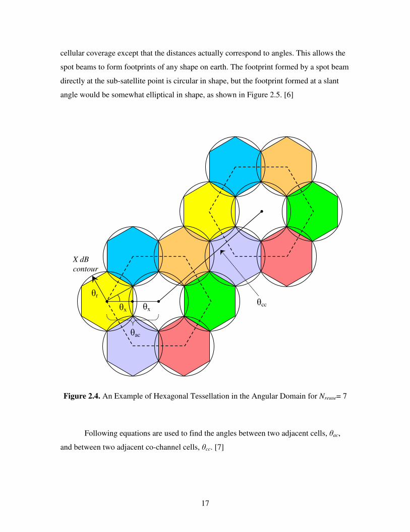
17

cellular coverage except that the distances actually correspond to angles. This allows the

spot beams to form footprints of any shape on earth. The footprint formed by a spot beam

directly at the sub-satellite point is circular in shape, but the footprint formed at a slant

angle would be somewhat elliptical in shape, as shown in Figure 2.5. [6]

Figure 2.4. An Example of Hexagonal Tessellation in the Angular Domain for Nreuse= 7

Following equations are used to find the angles between two adjacent cells, θac,

and between two adjacent co-channel cells, θcc. [7]

X dB

contour

θr

θx θx

θac

θcc

18

2

3.)30cos(. rrx θθθ == o (2.10)

xac θθ .2= (2.11)

3rac θθ =⇒ (2.12)

Similarly,

reusercc N.3θθ = (2.13)

Step 2

In this step, the angle each interferer makes with the boresight of the uplink

antenna’s spot beam, which serves the user earth station or mobile, is found along with

the different path lengths they have from the satellite.

The angular separation of the co-channel cells is calculated using the same

equations as in step 1, except that instead of using a cell reuse value of 1 to come up for

the entire coverage map, the actual cell reuse value is used. Three different placement

scenarios are considered for the interferers, namely, random, worst-case and best-case

placements. For all cases, the assumption that exactly one interferer exists in each co-

channel cell still stands.

For the random scenario, the interferers are randomly placed in the respective co-

channel cells. This is done by the use of a built-in random number generator function in

MATLAB. The interferers are randomly distributed in ‘ρ’, which appears to be the radius

of a cell in the angular domain based coverage map, but is actually the angular separation

between the interferer and the center of the spot beam. The value for ‘ρ’ varies between 0

and the X dB Beamwidth of the spot beam. The interferers are also randomly distributed

in ‘φ’, which varies from 0˚ to 360˚.

For the worst-case scenario, an interferer is placed at a point within the cell at

which the angular separation between it and the usercell’s center is such that the relative

19

antenna pattern contribution is the maximum possible from the interferer’s cell. In most

cases, the closer an interferer is to the usercell’s center, the more it can contribute

towards the interference power since the relative antenna pattern value of the usercell’s

spot beam is higher when close to the main lobe of the pattern.

For the best-case scenario, an interferer is placed at a point within the cell at

which the angular separation between it and the usercell’s center is such that the relative

antenna pattern contribution is the minimum possible from the interferer’s cell. Often

times, this would show that the angles are such that they fall in or are close to the nulls in

the antenna pattern.

The distribution of the cells in the angular domain, although simple, does require

that the co-channel interferers and the user earth station or mobile be defined or mapped

to the angular coverage map. The co-channel interferers are defined in the program in

terms of angles on the angular coverage map. On the other hand, the earth station/mobile

could be input one of two ways: 1) As Latitude and Longitude on the earth’s surface, or

2) As a point selected by the user on the angular coverage map created by the program.

Therefore, the program maps the user location, if input as Lat/Long, to the angular

coverage map. Since the co-channel interferers are on the earth surface and different

distances apart from the satellite, the co-channel interferers’ locations on the angular

coverage map need to be mapped to the earth’s surface.

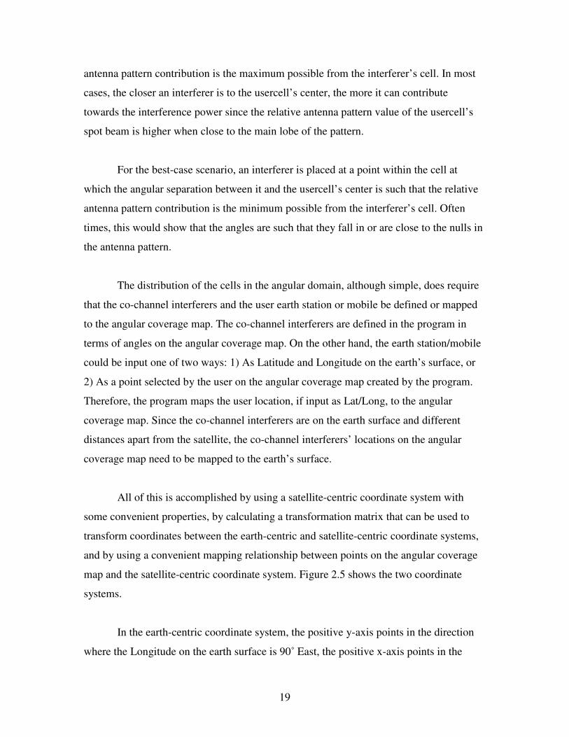
All of this is accomplished by using a satellite-centric coordinate system with

some convenient properties, by calculating a transformation matrix that can be used to

transform coordinates between the earth-centric and satellite-centric coordinate systems,

and by using a convenient mapping relationship between points on the angular coverage

map and the satellite-centric coordinate system. Figure 2.5 shows the two coordinate

systems.

In the earth-centric coordinate system, the positive y-axis points in the direction

where the Longitude on the earth surface is 90˚ East, the positive x-axis points in the

20

direction where the Longitude on the earth surface is 0˚, the x-y plane corresponds to the

equatorial plane, and the positive z-axis points in the direction where the Latitude on the

earth surface is 90˚ North. Whereas, in the satellite-centric coordinate system, the

positive z′-axis points in the direction of the line vector from satellite to the center of

coverage on the earth surface. For convenience and simplicity, the y′-axis is assumed to

have no x-component (in the earth-centric system), and the cross product of these two

axes produces the unit vector for the x′-axis.

Figure 2.5. Earth and Satellite Centric Coordinate Systems

T

Lat = 0˚ Long = 0˚

Lat = 0˚ Long = 90˚ E

Sub-Sat Pt.

Center of Coverage

z′-axis

x′ y′ plane

Lat = 90˚ N

Latsub-sat

RE O

y-axis

x-axis

z-axis

21

The equations used to define the satellite-centric coordinate system’s axes are

shown below.

)](),(),[( covcovcovcov2 satcntrsatcntrsatcntrcntrsat zzyyxxvz −−−=≡′rr

(2.14)

2

cov

2

cov

2

cov

covcovcov

)()()(

)](),(),[(ˆ

satcntrsatcntrsatcntr

satcntrsatcntrsatcntr

zzyyxx

zzyyxx

z

zz

−+−+−

−−−=

′

′≡′ r

r

(2.15)

Since the y′-axis is assumed to have no x-component, it can be calculated in one

of the following ways,

]1,0,0[≡′yr

if z′z = 0 (2.16)

or

]0,1,0[≡′yr

if z′y = 0 (2.17)

or

′

′−≡′

z

y

z

zy ,1,0r

for all other values (2.18)

y

yy

′

′=′⇒ r

r

ˆ (2.19)

Therefore, the unit vector for the positive x′-axis is given by,

yzx ′×′≡′ ˆˆˆ (2.20)

To convert a point in one coordinate system to the other, transformation and

translation of axes is done. The equations used are as follows:

−

×=

′

′

′

−

×

⋅′⋅′⋅′

⋅′⋅′⋅′

⋅′⋅′⋅′

=

′

′

′

t

a

a

a

T

O

O

O

a

a

a

zzyzxz

zyyyxy

zxyxxx

a

a

a

z

y

x

z

y

x

z

y

x

z

y

x

ˆˆˆˆˆˆ

ˆˆˆˆˆˆ

ˆˆˆˆˆˆ

(2.21)

22

Here, the rows of the 3x3 transformation matrix, T, represent the direction cosines

of the x′-axis, y′-axis and z′-axis, respectively, in the earth-centric coordinate system. The

3x1 translation matrix, t, represents the coordinates of the satellite in the earth-centric

coordinate system.

Given that coordinates for all points in the earth-centric system can be

transformed into coordinates in the satellite-centric system, a convenient mapping

relationship between points on the angular coverage map and the satellite-centric system

was used. Again for convenience, it is assumed that the angle that the projection of any

point in the satellite-centric system on the x′ y′ plane makes with the x′-axis is the same as

the angle the mapped point (on the angular coverage map) makes with the alpha-x-axis.

How far the mapped point is from the center of the coverage map is simply the angle in

degrees between it and the coverage center.

In order to calculate the distance between the satellite and the different interferers

on the earth surface, a user-defined function called ‘DIST_SAT2EARTH’ is used. This in

turn makes use of another user-defined function called ‘INTRSCTN_RAY2SPH’ to find

the closest point of intersection between a ray and the spherical earth.

Step 3

Using the angles that the interferers make with the boresight of the usercell’s spot

beam and the distances that the interferers are from the satellite, the relative pattern

values of the interferers and their respective path losses are found. Equation 2.7 is used

for the relative antenna pattern values. This leads to calculating the interference powers

for the three different scenarios, using the following general equations:

∑∑==

=

N

kk

kRX

scanmiscatmBO

RXTXTXN

k

k

d

f

LLLP

GGPI

12

2max

1 ..4

)(.

...

..

λ

π

θ (2.22)

23

∑

∑

=−−

−−−−−

=

+−−

−−++=

N

k k

kRX

dBscandBmisc

dBatmdBBOdBRXdBTXdBTX

dB

N

k

k

d

fLL

LPGGPI

1

max

1

..4

)(log.20

λ

π

θKK

KK

(2.23)

In the equations above, the denominator in the summation on the right hand side

of the equation represents the free space path loss, Lpath.

2.6 Calculation of Downlink Co-Channel Interference

The main objective of this part of the code is to calculate the interference received

at the earth station or mobile receiver from the downlink co-channel spot beams that use

the same exact frequency as the main downlink user earth station or mobile receiver. The

procedure followed for this calculation is similar to that of the uplink case except that

there are no different scenarios since the interferers here are the static co-channel spot

beams instead of other earth station or mobile users as in the uplink case, and that the

distance between each interfering source and the user receiver is the same as the distance

between the satellite and the user earth station or mobile receiver. This is evident from

Figure 1.1. To calculate interference powers for the downlink case, the following general

equations are used:

∑∑= −=

=

N

k scank

kRX

k

miscatmBO

RXTXTXN

k

kL

f

dLLP

GGPI

1

2

2

max

1

)(.

..4...

.. θ

λ

π (2.24)

∑

∑

= −

−

−−−−−

=

+

+−

−−++=

N

k scank

kRX

k

dBmisc

dBatmdBBOdBRXdBTXdBTX

dB

N

k

k

L

f

dL

LPGGPI

1

2

max

1

)(log.10

..4log.20

θ

π

λKK

KK

(2.25)

24

Chapter 3

LEO Interference Case with Reuse Numbers 3, 4, and 7

3.1 Overview

In this chapter the effects of reuse number, antenna pattern sidelobe level and

number of co-channel tiers on co-channel interference are investigated for an L-Band

Low Earth Orbit (LEO) satellite based two-way personal communications system. The

input parameters for this scenario were taken from page 140 of [3], and are as shown in

Table 3.1.

Table 3.1. Parameters and Values Used for a LEO Scenario

Satellite Parameters

Satellite/Platform Orbit and Altitude LEO, Altitude = 1800 km

Satellite Transmit Power including Output Back-Off ─ 10 dBW per channel per beam

Number of Spot Beams 37

Overlapping Coverage is at ─ 4 dB below the beam center

Uplink Frequency / Downlink Frequency 1650 MHz / 1550 MHz

Antenna Gain for both Uplink and Downlink 23 dBi

Receiver Noise Temperature 500 K

Atmospheric Losses 0.5 dB

Receiver Noise Bandwidth (IF Bandwidth) 4.8 kHz Mobile Terminal Parameters

Transmitter Output Power ─ 3 dBW

Antenna Gain (transmit and receive) 0 dBi


User Location in the Coverage Cell ─ 3 dB contour

For simplicity, the analysis here is shown for the cases where the uplink and

downlink user locations are selected on the Coverage Map only and are placed close to

the fringe of their coverage cells, where the loss in gain is approximately 3 dB. An

analysis using specific uplink and downlink user locations in Lat/Long is shown in

Appendices D, E and F.

25

3.2 Program Run Results

The computer code allows uplink and downlink users to be placed within the

same cell, but for simplicity, both the uplink and downlink users are placed on opposite

sides of the center of coverage. The computer code does not assume that the center of

coverage is the same as sub-satellite point. In case of a LEO, the sub-satellite point is for

an instant of time and would change with time. For this program run, the Latitudes and

Longitudes for the sub-satellite point and the center of coverage, respectively, are as

specified in Table 3.2 below. These values represent an approximate center of the United

States, and also imply that the center of coverage does not have to be at the sub-satellite

point for the program to work.

Table 3.2. LEO: Lat/Long for the Sub-Satellite Point and Center of Coverage

Location Type Site Latitude Longitude

Center of Coverage Wichita, KS 37.68735° N 97.34267° W

Sub-Satellite Point Ponca City, OK 36.72363° N 97.06881° W

The input values used in the Input Excel file are shown in Tables 3.3, 3.4 and 3.5

below.

Table 3.3. LEO: General Parameters and Their Sample Values

Use Same Cell Coverage for both Uplink & Downlink? (0=No; 1=Yes) 1

Latitude-Center of Coverage (in decimal degrees North) 37.68735

Longitude-Center of Coverage (in decimal degrees West) 97.34267







Latitude-Satellite (in decimal degrees North) 36.72363

Longitude-Satellite (in decimal degrees West) 97.06881


26

Table 3.4. LEO: Uplink Parameters and Their Sample Values










Mobile/Fixed ES TX Pwr (in dBW) -3

Mobile/Fixed ES TX Back-Off (in dBW) 0








Miscellaneous Losses for the Mobile/Fixed ES TX ONLY (in dB) 0




27

Table 3.5. LEO: Downlink Parameters and Their Sample Values










Sat TX Pwr (in dBW) -10

Sat TX Back-Off (in dBW) 0

Max. Gain of Sat TX Antenna (in dBi) 23

3-dB Beamwidth of Sat TX Antenna (in degrees) 12.8

Enter Taper Value for a circular aperture Sat TX Antenna (0, 1, 2) 1









The uplink and downlink user locations have been chosen to be in cells adjacent

to the center of coverage, but on opposite sides. This can be seen from Figure 3.1, which

shows the distribution of co-channel beam centers for the uplink & downlink along with

angular locations of the interferers.

28

Figure 3.1. LEO: Angular Distribution of Co-channel Beam Centers for the UPLINK & DOWNLINK for Reuse # 3

As mentioned in Chapter 2, in the uplink case, the computer code finds the worst

case interferers, best case interferers and randomly distributed interferers. The angles

these interferers make with the uplink user’s cell center are shown in Figure 3.2. Also

shown are the angles that the cell centers of the downlink interferers make with the

downlink user earth station or mobile.

29

Figure 3.2. LEO: Normalized Antenna Pattern of the UPLINK & DOWNLINK Satellite Antennas for a Uniform Illumination

Sample runs of the computer code for the aforementioned LEO system parameters

are shown in Tables 3.6 and 3.7. Table 3.6 shows the worst case, best case and random

case CNIR values when the antenna sidelobe levels (SLLs) for both the uplink and

downlink satellite antennas is -17.6 dB, which corresponds to a uniform illumination

distribution function. On the other hand, in order to show the variation in CIR and CNIR

due to antenna sidelobe levels, Table 3.7 shows sample runs of the program for only the

randomly distributed uplink interferers, but for different sidelobe levels of the satellite

uplink and downlink antennas, and also for different co-channel tiers.

30

Table 3.6. LEO: Worst Case, Best Case, and Random case CNIR values

Downlink

(CNR = 14.6 dB)

Uplink

(CNR = 18.9 dB)

Overall

(CNR = 13.2 dB) Reuse

CIR (dB)

CIRWC

(dB) CIRBC

(dB) CIRRDM

(dB) CNIRWC

(dB) CNIRBC

(dB) CNIRRDM

(dB)

3 9.5 6.8 28.0 8.9 4.3 7.9 5.4

4 9.7 7.2 86.1 10.5 4.6 8.1 6.1

7 16.4 16.4 75.1 16.7 10.3 11.5 10.4

Table 3.7. LEO: Sample Runs of the Program for the Random Case only

Downlink

(CNR = 14.6 dB)

Uplink

(CNR = 18.9 dB)

Overall

(CNR = 13.2 dB) Reuse Sidelobe

Level (dB)

Tiers CIR (dB)

Tiers CIRRDM

(dB) CNIRRDM

(dB)

3 2 9.5 2 8.9 5.4

4 2 9.7 2 10.5 6.1

7

─ 17.6

1 16.4 1 16.7 10.4

3 2 17.1 2 17.3 10.7

4 2 17.4 2 18.8 11.0

7

─ 24.6

1 28.7 1 27.8 12.9

3 2 19.4 2 24.0 12.0

4 2 24.2 2 24.4 12.6

7

─ 30.6

1 37.1 1 38.0 13.2

3 1 17.4 1 17.6 10.8

4 ─ 24.6

1 17.5 1 18.8 11.0

31

Chapter 4

GEO Interference Case with Reuse Numbers 3, 7, and 13

4.1 Overview

In this chapter the effects of reuse number, antenna pattern sidelobe level and

number of co-channel tiers on co-channel interference are investigated for an L-Band

Geostationary Earth Orbit (GEO) satellite based two-way personal communications

system. The input parameters for this scenario were taken from an FCC application for a

GEO space station at 63.5° W by Mobile Satellite Ventures Subsidiary LLC and are as

shown in Table 4.1. [8]

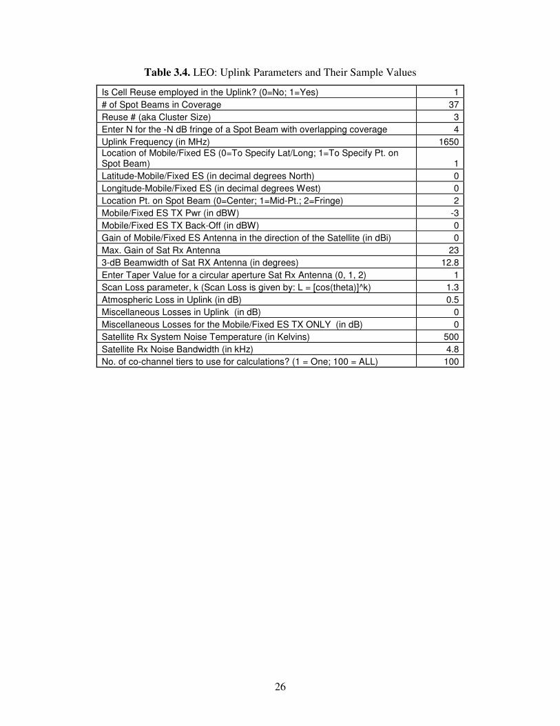
Table 4.1. Parameters and Values Used for a GEO Scenario

Satellite Parameters

Satellite/Platform Orbit and Altitude GEO, Altitude = 35786 km

Satellite Transmit Power including Output Back-Off 10.9 dBW per carrier per beam

Number of Spot Beams 127

Overlapping Coverage is at ─ 4 dB below the beam center

Uplink Frequency / Downlink Frequency 1640 MHz / 1550 MHz

Antenna Gain for both Uplink and Downlink 47 dBi


Atmospheric Loss 0.5 dB

Miscellaneous Losses for Uplink/Downlink 2.2 dB / 7 dB

Carrier Noise Bandwidth for Uplink/Downlink 50 kHz / 200 kHz Mobile Terminal Parameters

Transmitter Output Power 0 dBW

Antenna Gain (transmit and receive) ─ 4 dBi


User Location in the Coverage Cell ─ 3 dB contour

For simplicity, the analysis here is shown for the cases where the uplink and

downlink user locations are selected on the Coverage Map only and are placed close to

the fringe of their coverage cells, where the loss in gain is approximately 3 dB. An

analysis using specific uplink and downlink user locations in Lat/Long is shown in

Appendices D, E and F.

32

4.2 Program Run Results

As mentioned in the previous chapter, the computer code allows uplink and

downlink users to be placed within the same cell, but for simplicity, both the uplink and

downlink users are placed on opposite sides of the center of coverage. The computer code

does not assume that the center of coverage is the same as sub-satellite point.

In this program run, for simplicity, the location of the sub-satellite point and the

center of coverage are the same and are as specified in Table 4.2 below. The GEO

satellite in [8] is intended to provide coverage to South America, but due to the chosen

location of center of coverage and the 127 spot beams, the actual coverage area is

hexagonal in appearance and may not cover the South American region as intended by

GEO satellite in [8]. Only 127 spot beams were chosen for analysis here in order to show

a legible figure for the coverage map generated by the program, whereas 217 or even

more spot beams could be accommodated in the earth’s view from this GEO satellite.

Table 4.2. GEO: Lat/Long for the Sub-Satellite Point and Center of Coverage

Location Type Site Latitude Longitude

Center of Coverage Near the City of Manaus, Brazil, South America

0° N 63.5° W

Sub-Satellite Point same as above 0° N 63.5° W

The values used in the Input Excel file are shown in Tables 4.3, 4.4 and 4.5

below.

33

Table 4.3. GEO: General Parameters and Their Sample Values



Longitude-Center of Coverage (in decimal degrees West) 63.5








Longitude-Satellite (in decimal degrees West) 63.5


Table 4.4. GEO: Uplink Parameters and Their Sample Values










Mobile/Fixed ES TX Pwr (in dBW) 0

Mobile/Fixed ES TX Back-Off (in dBW) 0








Miscellaneous Losses for the Mobile/Fixed ES TX ONLY (in dB) 0


Satellite Rx Noise Bandwidth (in kHz) 50


34

Table 4.5. GEO: Downlink Parameters and Their Sample Values










Sat TX Pwr (in dBW) 10.9

Sat TX Back-Off (in dBW) 0

Max. Gain of Sat TX Antenna (in dBi) 47

3-dB Beamwidth of Sat TX Antenna (in degrees) 0.81

Enter Taper Value for a circular aperture Sat TX Antenna (0, 1, 2) 0







Mobile/Fixed ES Rx Noise Bandwidth (in kHz) 200


The uplink and downlink user locations have been chosen to be in cells adjacent

to the center of coverage, but on opposite sides. This can be seen from Figure 4.1, which

shows the distribution of co-channel beam centers for the uplink & downlink along with

angular locations of the interferers for a case with a reuse number of 7. A reuse number

equal to 7 was chosen to be able to clearly show the co-channel cells along with the

positions of the interferers.

35

Figure 4.1. GEO: Angular Distribution of Co-channel Beam Centers for the UPLINK & DOWNLINK for Reuse # 7

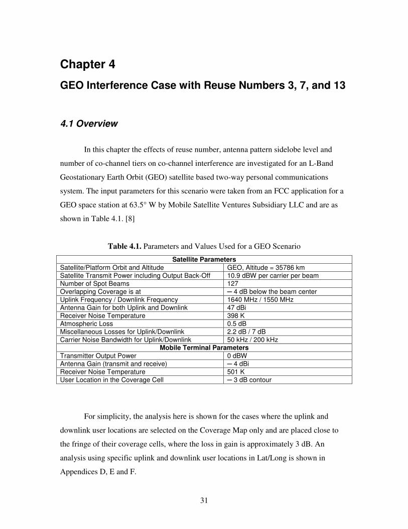
As mentioned in Chapter 2, for the uplink case, the computer code finds the worst

case interferers, best case interferers and randomly distributed interferers. The angles

these interferers make with the uplink user’s cell center are shown in Figure 4.2. Also

shown are the angles that the cell centers of the downlink interferers make with the

downlink user earth station or mobile.

36

Figure 4.2. GEO: Normalized Antenna Pattern of the UPLINK & DOWNLINK Satellite Antennas for a Uniform Illumination

Sample runs of the computer code for the aforementioned GEO system

parameters are shown in Tables 4.6 and 4.7. Table 4.6 shows the worst case, best case

and random case CNIR values when the antenna sidelobe levels (SLLs) for both the

uplink and downlink satellite antennas is -17.6 dB, which corresponds to a uniform

illumination distribution function. On the other hand, in order to show the variation in

CIR and CNIR due to antenna sidelobe levels, Table 4.7 shows sample runs of the

program for only the randomly distributed uplink interferers, but for different sidelobe

levels of the satellite uplink and downlink antennas, and also for different co-channel

tiers.

37

Table 4.6. GEO: Worst Case, Best Case, and Random case CNIR values

Downlink

(CNR = 15.7 dB)

Uplink

(CNR = 11.3 dB)

Overall

(CNR = 10.0 dB) Reuse

CIR (dB)

CIRWC

(dB) CIRBC

(dB) CIRRDM

(dB) CNIRWC

(dB) CNIRBC

(dB) CNIRRDM

(dB)

3 9.2 5.2 49.3 7.6 2.8 6.6 4.0

7 16.4 12.0 55.0 14.4 7.3 9.1 8.0

13 21.2 17.0 51.2 19.7 8.9 9.7 9.3

Table 4.7. GEO: Sample Runs of the Program for the Random Case only

Downlink

(CNR = 15.7 dB)

Uplink

(CNR = 11.3 dB)

Overall

(CNR = 10.0 dB) Reuse Sidelobe

Level (dB)

Tiers CIR (dB)

Tiers CIRRDM

(dB) CNIRRDM

(dB)

3 4 9.2 4 7.6 4.0

7 3 16.4 3 14.4 8.0

13

─ 17.6

2 21.2 2 19.7 9.3

3 4 17.5 4 16.7 8.6

7 3 27.2 3 27.4 9.8

13

─ 24.6

2 32.3 2 33.5 9.9

3 4 20.6 4 23.7 9.5

7 3 36.0 3 36.6 10.0

13

─ 30.6

2 43.2 2 42.8 10.0

3 1 18.2 1 17.1 8.7

7 1 27.8 1 27.7 9.8

13

─ 24.6

1 32.5 1 33.6 9.9

38

Chapter 5

Conclusions, Limitations and Future Work

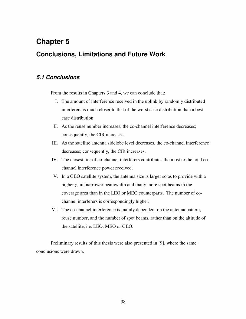
5.1 Conclusions

From the results in Chapters 3 and 4, we can conclude that:

I. The amount of interference received in the uplink by randomly distributed

interferers is much closer to that of the worst case distribution than a best

case distribution.

II. As the reuse number increases, the co-channel interference decreases;

consequently, the CIR increases.

III. As the satellite antenna sidelobe level decreases, the co-channel interference

decreases; consequently, the CIR increases.

IV. The closest tier of co-channel interferers contributes the most to the total co-

channel interference power received.

V. In a GEO satellite system, the antenna size is larger so as to provide with a

higher gain, narrower beamwidth and many more spot beams in the

coverage area than in the LEO or MEO counterparts. The number of co-

channel interferers is correspondingly higher.

VI. The co-channel interference is mainly dependent on the antenna pattern,

reuse number, and the number of spot beams, rather than on the altitude of

the satellite, i.e. LEO, MEO or GEO.

Preliminary results of this thesis were also presented in [9], where the same

conclusions were drawn.

39

5.2 Limitations and Future Work

The computer code has the following limitations which can be overcome in future

work. Some additions can be made without changing the code much, but a change in the

design philosophy of the code will require a complete rewrite.

a) It only uses a single satellite for analysis.

b) Antenna pattern files can not be input.

c) Only choice in antenna pattern is in its taper values.

d) Coverage map can only be a hexagonal in geometry.

e) Antenna patterns do not vary according to scan angle; rather, they are

assumed to be the same for all spot beams.

f) The scan loss parameter only reduces the gain value of the antenna based

on the scan angle, but does not assume a changed relative antenna pattern.

g) Earth is assumed to be a spheroid, and not an ellipsoid; therefore, there’s

an inherent (minor) error in converting a Lat/Long value into xyz-

coordinates.

h) Spot beams are not shown on the map/globe of earth.

i) The program doesn’t have a Graphical User Interface (GUI).

j) The program doesn’t work for a CDMA system, but only for

FDMA/TDMA systems.

k) The calculation for overall CNR or CNIR assumes a linear (bent-pipe)

satellite transponder. For a transponder with OBP and FEC coding, the

overall CNR or CNIR is not an accurate measure of performance. In such

a case, the link CNIRs should be used to calculate the respective link

BERs.

l) Using digital modulation, FEC coding and OBP are some methods of

improving the system performance. Yet another method is to improve the

antenna pattern such that the pattern nulls coincide with the first and

second tier of the co-channel beams. [10]

40

References

[1] A.I. Zaghloul and O. Kilic, “Transmission Impairment Parameters in Multiple-

Beam Satellite Communications Systems,” URSI General Assembly, Maastricht, The Netherlands, August 2002.

[2] United States. National Communications System Technology & Standards

Division, “Telecommunications: Glossary of Telecommunication Terms,” Federal Standard 1037C, August 1996, < http://www.its.bldrdoc.gov/fs-1037/>.

[3] T. Pratt, C. Bostian and J. Allnutt, “Satellite Communications,” 2nd ed., pp. 128, 137-144, 2003.

[4] Tri T. Ha, “Digital Satellite Communications,” 2nd ed., pp. 138-157, 1990. [5] W. L. Stutzman and G.A. Thiele, “Antenna Theory and Design,” 2nd ed., pp. 320,

1998. [6] A.I. Zaghloul, F.T. Assal, B.H. Hutchinson and E. Jurkiewicz, “Satellite

Communications to Hand-Held Terminals from Geostationary Orbit,” 9th International Conference on Digital Satellite Communications, Copenhagen, Denmark, May 18-22, 1992.

[7] S. K. Rao, “Parametric Design and Analysis of Multiple-Beam Reflector Antennas

for Satellite Communications,” IEEE Antennas and Propagation Magazine, Vol. 45, No. 4, August 2003.

[8] FCC File Number: SAT-AMD-20040227-00021, “Amendment to Application for

Authority to Launch and Operate an L-band Mobile Satellite Service Satellite at

63.5°W,” Mobile Satellite Ventures Subsidiary LLC, February 2004, Authority Granted on January 10, 2005.

[9] S. Chhabra, A.I. Zaghloul and O. Kilic, “Co-Channel Interference in Satellite-

Based Cellular Communication Systems,” URSI General Assembly, New Delhi, India, October 2005.

[10] O. Kilic, A. I. Zaghloul, M. Thai, L. Nguyen, "Beam Interference Modeling in

Cellular Satellite Communication Systems," URSI General Assembly Meeting, 1999.

41

Appendix A

Program Flow for the Computer Code

This appendix presents a detailed program flow for the computer code developed in

this thesis.

I. Read inputs for Uplink, Downlink & General Parameters from the Excel file.

II. Uplink Calculations � Plot the Uplink Antenna Pattern

� Use the 3-dB beamwidth provided and the N for the -N dB fringe � Do the Satellite Visibility & elevations tests for the coverage center � Draw the coverage map (even if it's only 1 cell, i.e. no reuse)

� Draw the circles around the beam centers to show beams' angular boundaries

� Check to see if any coverage cell falls off the earth's curvature � If the user location is specified in Lat/Long,

� do the Satellite Visibility & Elevation tests � Find the projection of the user location in the Coverage Map � Make sure the user (its projection) is within the coverage area

� Else if the user location is selected on the coverage map � Find the closest beam center not more than 0.5 x Beamwidth away � Re-define user location in its coverage cell according to the user-

specified location in the Excel input file � Display the user location on the coverage map

� If reuse is done in UL, � Find co-channel cells in coverage � Find relative pattern values for one user in each co-channel cell for

interferers: � distributed randomly � distributed in a manner they contribute the most power

(W.C.) � distributed in a manner they contribute the least power

(B.C.) � *** NOTE: show these on the antenna pattern plot & the

coverage map � *** NOTE: Same scan loss value is used for the user & all

interferers � Find the distance between each interferer & the sat to get path loss

values

42

� Add up the respective antenna pattern values divided by path loss values, as explained by the equation used for summing the interference powers

� Add these values calculated above to find the total interference power received by the satellite for the different interference scenarios

� Find the user power received at the satellite � Find the path loss for the user � Find the relative antenna pattern value for the user since it can be

anywhere in the cell � Add up all contributions to get the carrier power received

� Find the noise power using the system noise temperature & noise bandwidth

� Find the CNR � If reuse is done in UL,

� Calculate the uplink CIRs & CNIRs for the different interference scenarios

� Find the CNIR (CNIR = CNR if no reuse is done in UL) III. Downlink Calculations

� If the reuse is same for the uplink and the downlink, � Following parameters will be the same as those for the uplink:

� No. of cells, Coverage Cells, Satellite antenna gain, the 3-dB beamwidth and the taper value for the satellite antenna pattern

� Else if the reuse is different, � Plot the Uplink Antenna Pattern

� Use the 3-dB beamwidth provided and the N for the -N dB fringe

� Do the Satellite Visibility & Elevation tests for the coverage center � Draw the coverage map (even if it's only 1 cell, i.e. no reuse)

� Draw the circles around the beam centers to show beams' angular boundaries

� Check to see if any coverage cell falls off the earth's curvature

� If the user location is specified in Lat/Long, � do the Satellite Visibility & Elevation tests � Find the projection of the user location in the Coverage Map � Make sure the user (its projection) is within the coverage area

� Else if the user location is selected on the coverage map � Find the closest beam center not more than 0.5 x Beamwidth away � Re-define user location in its coverage cell according to the user-

specified location in the Excel input file � Display the user location on the coverage map

� Find the path loss for the user (it's the same for the co-channel interferers) � If reuse is done in DL,

43

� Find co-channel cells in coverage � Find relative pattern values for the angles made between the user

and each of the co-channel beam centers � *** NOTE: show these on the antenna pattern plot

� Find the different scan loss values for each of the co-channel beams

� Add up the respective antenna pattern values divided by scan loss values, as explained by the equation used for summing the interference powers

� Add these values calculated above to find the total interference power received by the downlink user

� Find the power received by the downlink user � Find the relative antenna pattern value for the user since it can be

anywhere in the cell � Add up all contributions to get the carrier power received

� Find the noise power using the system noise temperature & noise bandwidth

� Find the CNR � If reuse is done in DL,

� Calculate the uplink CIRs & CNIRs for the different interference scenarios

� Find the CNIR (CNIR = CNR if no reuse is done in DL) IV. Calculations for the overall CNR, CNIR (degradation to CNR)

� Calculate the overall CNR using both UL & DL CNR values � Calculate the overall CNIR using both UL & DL CNIR values

44

Appendix B

Main Computer Code

This appendix presents the main computer code developed in MATLAB for the

analysis of the scenarios discussed in this thesis.

This work (thesis and code) is copyrighted as mentioned on the cover sheet.

%%%%%%%%%%%%%%%%%%%%%%%%%%%%%%%%%%%%%%%%%%%%%%%%%%%%%%%%%%%%%%%%%%% % This program calculates the co-channel interference for a single % satellite system that employs frequency reuse through the use % of spot beams. It calculates the Overall CNIR and the degradation % in CNR caused by co-channel interference in satellite spot-beams. % It tackles the uplink and downlink scenarios separately. % % Input Parameters and their values are taken from an MS Excel % file called 'Input2Program.xls' by default. % % User-defined functions used: % lat2xyz, plot_ant_pattern, visibNelev_test, plot_coverage_map, % arc_length, co_ch_pts, proj2alpha_xy, intrsctn_ray2sph, % dist_sat2earth, co_ch_ang_mtx, pattern_value, ktb_dBW. % % MATLAB code developed by SAURBH CHHABRA % Copyright 2006, Saurbh Chhabra % Date updated: August 20, 2006 %%%%%%%%%%%%%%%%%%%%%%%%%%%%%%%%%%%%%%%%%%%%%%%%%%%%%%%%%%%%%%%%%%% % % Start Of Program clear all close all format short g global earth_radius sat_ht_abv_earth sat_lat_deg sat_long_deg minElev % disp(' ') disp('=============================================================') disp(' PROGRAM TO CALCULATE CO-CHANNEL INTERFERENCE IN A FREQUENCY') disp(' REUSE SINGLE-SATELLITE-BASED COMMUNICATIONS SYSTEM') disp('=============================================================') disp(' ')

45

disp('**************************************************************') disp('Assumptions made: ') disp(' ') disp(' Earth is spherical in shape.') disp(' Spot beams are for a single satellite or elevated platform') disp(' based system.') disp(' Beamwidths for all spot beams of a link are the same. ') disp(' The relative antenna patterns for all spot beams of a link ') disp(' are the same.') disp(' Cells are distributed in an angular fashion, and the cell') disp(' centers in any tier form a hexagon in the angular domain.') disp(' The satellite transmit power is the same for all spot beams. ') disp(' The source signal transmit power and antenna gain are the ') disp(' same for the user and the interferers of a link. In other') disp(' words, if the uplink user is a mobile, then the uplink') disp(' interferers are mobiles with the same transmit power and') disp(' antenna gain as the user mobile.') disp(' There is only one interferer in each co-channel cell that') disp(' actively transmits at the main user''s frequency.') disp(' The calculations are not for a CDMA system.') disp('**************************************************************') % %%%%%%%%%%%%%%%%%%%%%%%%%%%%%%%%% % GENERAL INPUTS & CALCULATIONS %%%%%%%%%%%%%%%%%%%%%%%%%%%%%%%%% % % CONSTANTS: c = 3*(10^8); % in meters/second earth_radius = 6378.137; % in km geo_height = 35786.033; % km % % INPUTS: % Following allows the user to enter the INPUT filename dlg_prompt = 'Enter the Excel file name:'; dlg_title = 'MS Excel file used as Input for the Program'; lines = 1; def_input = {'Input2Program_GEO_MSV_SA.xls'}; % A cell array is formed by the inputdlg function below InputFile_ca = inputdlg(dlg_prompt, dlg_title, lines, def_input); % Changes the cell array to a string that can be used with the % xlsread function InputFile = char(InputFile_ca); disp(' ') disp(' ') disp('---------------------') disp(' General Input Data') disp('---------------------') disp(' ') disp(' ') [GeneralData, GeneralTxt] = xlsread(InputFile, 'General'); %

46

% Assigning variables to input data disp(' ') % Use Same Coverage Cells for both Uplink & Downlink? (0=No; 1=Yes) GeneralTxt(1) UseSameCellsUpNDown = GeneralData(1) if UseSameCellsUpNDown == 1 % Latitude-Center of Coverage (in decimal degrees) GeneralTxt(2) cov_cntr_lat_deg = GeneralData(2) % Longitude-Center of Coverage (in decimal degrees) GeneralTxt(3) cov_cntr_long_deg = GeneralData(3) % Latitude-Center of Coverage for Uplink (in decimal degrees) UL_cov_cntr_lat_deg = cov_cntr_lat_deg % Longitude-Center of Coverage for Uplink (in decimal degrees) UL_cov_cntr_long_deg = cov_cntr_long_deg % Latitude-Center of Coverage for Downlink (in decimal degrees) DL_cov_cntr_lat_deg = cov_cntr_lat_deg % Longitude-Center of Coverage for Downlink (in decimal degrees) DL_cov_cntr_long_deg = cov_cntr_long_deg else % Latitude-Center of Coverage (in decimal degrees) cov_cntr_lat_deg = 0 % Longitude-Center of Coverage (in decimal degrees) cov_cntr_long_deg = 0 % Latitude-Center of Coverage for Uplink (in decimal degrees) GeneralTxt(4) UL_cov_cntr_lat_deg = GeneralData(4) % Longitude-Center of Coverage for Uplink (in decimal degrees) GeneralTxt(5) UL_cov_cntr_long_deg = GeneralData(5) % Latitude-Center of Coverage for Downlink (in decimal degrees) GeneralTxt(6) DL_cov_cntr_lat_deg = GeneralData(6) % Longitude-Center of Coverage for Downlink (in decimal degrees) GeneralTxt(7) DL_cov_cntr_long_deg = GeneralData(7) end % Is the satellite in GEO? (0=No, 1=Yes) GeneralTxt(8) IsGEO = GeneralData(8) disp(' A 1 means the Satellite is in GEO'); disp(' ') if IsGEO==1 sat_ht_abv_earth = geo_height % in km sat_lat_deg = 0 else % Satellite-Height above Earth (in km) GeneralTxt(9) sat_ht_abv_earth = GeneralData(9) % Latitude-Satellite (in decimal degrees)

47

GeneralTxt(10) sat_lat_deg = GeneralData(10) end % Longitude-Satellite (in decimal degrees) GeneralTxt(11) sat_long_deg = GeneralData(11) % Minimum elevation angle for the Satellite Visibility Test GeneralTxt(12) minElev = GeneralData(12) % in degrees % Converts values to units that can be easily used UL_cov_cntr_lat_sec = UL_cov_cntr_lat_deg*3600; UL_cov_cntr_long_sec = UL_cov_cntr_long_deg*3600; DL_cov_cntr_lat_sec = DL_cov_cntr_lat_deg*3600; DL_cov_cntr_long_sec = DL_cov_cntr_long_deg*3600; sat_lat_rad = sat_lat_deg*pi/180; sat_lat_sec = sat_lat_deg*3600; sat_long_rad = sat_long_deg*pi/180; sat_long_sec = sat_long_deg*3600; % % %%%%%%%%%%%%%%%%%%%%%%%%%%%%%%% % UPLINK INPUTS & CALCULATIONS %%%%%%%%%%%%%%%%%%%%%%%%%%%%%%% % disp(' ') disp(' ') disp('---------------------') disp(' Uplink Input Data') disp('---------------------') disp(' ') [UplinkData, UplinkTxt] = xlsread(InputFile, 'Uplink'); % % Assigning variables to input data % % Is Cell Reuse employed in the Uplink? (0=No; 1=Yes) IsReuseUsed4Uplink = UplinkData(1) if IsReuseUsed4Uplink == 1 % # of Spot Beams in Coverage UL_num_beams = UplinkData(2) % Reuse # (aka Cluster Size) UL_reuse_num = UplinkData(3) else UL_num_beams = 1 % Reuse # (aka Cluster Size) UL_reuse_num = 1 end % Enter N for the -N dB fringe of a Spot Beam with overlapping coverage UL_XdB_fringe = UplinkData(4) % Uplink Frequency (in MHz) UL_freq_MHz = UplinkData(5) % Location of Mobile/Fixed ES (0=To Specify Lat/Long; 1=To Specify Pt. on Spot Beam)

48

UL_es_loc = UplinkData(6) % Latitude-Mobile/Fixed ES (in decimal degrees) UL_es_lat_deg = UplinkData(7) % Longitude-Mobile/Fixed ES (in decimal degrees) UL_es_long_deg = UplinkData(8) % Location Pt. on Spot Beam (0=Center; 1=Mid-Pt.; 2=Fringe) UL_es_loc_on_spot_beam = UplinkData(9) % Mobile/Fixed ES Tx Pwr (in dBW) UL_es_tx_pwr_dBW = UplinkData(10) % Mobile/Fixed ES Tx Back-Off (in dBW) UL_es_tx_bo_dBW = UplinkData(11) % Max. Gain of Mobile/Fixed ES Antenna (in dBi) UL_es_ant_gain_dBi = UplinkData(12) % Max. Gain of Sat Rx Antenna UL_sat_ant_gain_dBi = UplinkData(13) % 3-dB Beamwidth of Sat RX Antenna (in degrees) UL_sat_ant_bw_deg = UplinkData(14) UL_sat_ant_bw_rad = UL_sat_ant_bw_deg*pi/180; % Enter Taper Value for a circular aperture Sat Rx Antenna (0, 1, 2) UL_sat_ant_taper = UplinkData(15) % Scan Loss parameter, k for L = 10*k*log[cos(theta)] UL_scan_loss_k = UplinkData(16) % Atmospheric Loss (in dB) UL_atm_loss_dB = UplinkData(17) % Miscellaneous Losses (in dB) UL_misc_loss_dB = UplinkData(18) % Miscellaneous Losses for the Mobile/Fixed ES Tx ONLY (in dB) UL_misc_loss_es_dB = UplinkData(19) % Satellite Rx System Noise Temperature (in Kelvins) UL_SysNoiseTemp_K = UplinkData(20) % Satellite Rx Noise Bandwidth (in kHz) UL_NoiseBW_kHz = UplinkData(21) % No. of co-channel cells to use for calculations? (1 = One; 100 = ALL) UL_tiers2use = UplinkData(22) % % Converting Lat/Long to cartesian coordinates xyz_sat = lat2xyz(sat_lat_deg, sat_long_deg, sat_ht_abv_earth); xyz_subsat = lat2xyz(sat_lat_deg, sat_long_deg, 0); % % Uplink Frequency & Wavelength UL_freq_Hz = UL_freq_MHz*(10^6); % in Hz UL_lambda = c/UL_freq_Hz; % in m UL_lambda_km = UL_lambda/1000; % in km % % Plots the radiation pattern, calculates beta*a and the XdB beamwidth, which is used % to generate the coverage map in the angular domain % Finds the max angle for which the pattern value should be calculated; this is half the % max angle a satellite can subtend for the full view of the earth; pattern values are % calculated for more than this max angle for convenience in viewing the pattern. earth_view_ang_deg = 2*asin(earth_radius/(earth_radius+sat_ht_abv_earth))*180/pi; UL_theta_max_deg = 0.5*earth_view_ang_deg;

49

[UL_ant_bw_XdB_deg, UL_beta_a_sat, UL_ant_pat_handle] = plot_ant_pattern(UL_sat_ant_taper, ... UL_XdB_fringe, UL_sat_ant_bw_deg, UL_theta_max_deg); UL_ant_pat_lgnd = 'Pattern Data'; UL_ant_pat_title = 'Normalized Power Gain Pattern of the UPLINK Satellite Antenna'; title(UL_ant_pat_title); ylabel(' Relative Pattern Value in dB '); xlabel(' Angle Theta in degrees '); % % Plots the coverage map on a plane where (x,y) positions actually correspond to % angles, and so, the distance between any point and the origin is the angle that % cell center makes with the line joining the satellite & the center of coverage. % % Converting Lat/Long to cartesian coordinates for use later UL_xyz_cov_cntr = lat2xyz(UL_cov_cntr_lat_deg, UL_cov_cntr_long_deg, 0); % % Coverage Center Visibility Test UL_cov_cntr_lat_rad = UL_cov_cntr_lat_deg*pi/180; UL_cov_cntr_long_rad = UL_cov_cntr_long_deg*pi/180; sat_lat_rad = sat_lat_deg*pi/180; sat_long_rad = sat_long_deg*pi/180; [UL_dist_sat2covcntr_km, isvisib] = visibNelev_test(UL_cov_cntr_lat_rad, ... UL_cov_cntr_long_rad); % [UL_alpha_xy_N1, UL_cell_ang_dist_mtx, UL_T, UL_cov_map_handle] = plot_coverage_map... (xyz_sat, xyz_subsat, UL_xyz_cov_cntr, UL_num_beams, UL_reuse_num, UL_ant_bw_XdB_deg); % UL_cov_map_lgnd = 'Beam Center'; UL_cov_map_title = 'Co-channel Beam Centers for the UPLINK'; title(UL_cov_map_title); xlabel('Alpha y-axis (degrees)'); ylabel('Alpha x-axis (degrees)'); % UL_theta_radius_deg = UL_cell_ang_dist_mtx(1,1); UL_theta_cntr2cntr_deg = UL_cell_ang_dist_mtx(2,1); UL_theta_cochannel_deg = UL_cell_ang_dist_mtx(3,1); % % Draws the circular beam perimeter (in angular domain) around the cell centers % This code is placed here so that the legend labels aren't needed for these circles UL_theta = -0.01:0.01:2*pi; UL_r = UL_theta_radius_deg*ones(1,length(UL_theta)); [UL_ycell_perimtr, UL_xcell_perimtr] = pol2cart(UL_theta, UL_r); UL_x_y_cntrs = [UL_alpha_xy_N1(:,1), UL_alpha_xy_N1(:,2)]; for UL_cell_no = 1:size(UL_x_y_cntrs,1) UL_xcell_perimtr2(UL_cell_no,:) = UL_xcell_perimtr + UL_x_y_cntrs(UL_cell_no,1); UL_ycell_perimtr2(UL_cell_no,:) = UL_ycell_perimtr + UL_x_y_cntrs(UL_cell_no,2); end figure(UL_cov_map_handle) hold on

50

UL_h_circles = plot(UL_ycell_perimtr2', UL_xcell_perimtr2', 'b'); % if UL_es_loc == 0 % 0 is to specify Lat/Long for ES location % Conversion to units that are more useful UL_es_lat_rad = UL_es_lat_deg*pi/180; % in radians UL_es_long_rad = UL_es_long_deg*pi/180; % in radians % [UL_dist_sat2es_km, isvisib] = visibNelev_test(UL_es_lat_rad, UL_es_long_rad) % Uses a custom function 'lat2xyz' to convert Lat/Long to XYZ UL_xyz_es = lat2xyz(UL_es_lat_deg, UL_es_long_deg, 0); % % Projects the user location to the alpha_xy coordinate system using % the custom function 'proj2alpha_xy'; this also checks to make sure % that the ES falls within the defined coverage radius [UL_alpha_xy_escellcntr, UL_alpha_xy_es, IsULesInCoverage] = ... proj2alpha_xy(xyz_sat, UL_xyz_es, UL_xyz_cov_cntr, UL_alpha_xy_N1,... UL_T, UL_theta_radius_deg); figure(UL_cov_map_handle) hold on plot(UL_alpha_xy_es(2), UL_alpha_xy_es(1), 'pk', 'MarkerSize', 10.5); UL_cov_map_lgnd = strvcat(UL_cov_map_lgnd, 'Uplink User') % % Angle between ES and ES-cell's center; to be used to calculate % f_theta_es later UL_ang_es2escellcntr_deg = ... sqrt((UL_alpha_xy_escellcntr(:,2) - UL_alpha_xy_es(2)).^2 + ... (UL_alpha_xy_escellcntr(:,1) - UL_alpha_xy_es(1)).^2); % if IsULesInCoverage == 0 error(' The user is not in the coverage area'); end else % UL_es_loc == 1 is to select the ES location on the coverage map % Getting location info for the Uplink Earth Station figure(UL_cov_map_handle) hold on UL_h_msgBox= msgbox(... 'Click on the desired location for the UPLINK Earth Station.',... 'Figure Input Dialog Box'); uiwait(UL_h_msgBox) uiresume(UL_cov_map_handle) UL_alpha_xy_es_input = ginput(1); % in degrees % Swap X & Y to match the norm in this program UL_alpha_xy_es = [UL_alpha_xy_es_input(2) UL_alpha_xy_es_input(1)]; UL_h_ini_user_loc = plot(UL_alpha_xy_es(2), UL_alpha_xy_es(1), '+b'); % Finds coverage cell center closest to this point NOT greater than 0.5*bw UL_ang_es2cellcntrs_deg = sqrt((UL_alpha_xy_N1(:,2) - UL_alpha_xy_es(2)).^2 +... (UL_alpha_xy_N1(:,1) - UL_alpha_xy_es(1)).^2); [UL_ang_es2cellcntrs_min_deg, min_index] = min(UL_ang_es2cellcntrs_deg); if UL_ang_es2cellcntrs_min_deg > (0.5*UL_ant_bw_XdB_deg) disp(' ') error(' The selected user location is outside the closest coverage cell')

51

disp(' ') else UL_alpha_xy_escellcntr = UL_alpha_xy_N1(min_index, 1:2); end % Finds Theta & Rho for the user input with 'UL_alpha_xy_escellcntr' as % origin; this makes it simpler to place user at desired location in cell UL_alpha_xy_es_wrt_escellcntr = UL_alpha_xy_es - UL_alpha_xy_escellcntr; % Converts cartesian to polar % [TH,R] = CART2POL(X,Y) [UL_theta_es_wrt_escellcntr_rad, UL_rho_es_wrt_escellcntr_deg] =... cart2pol(UL_alpha_xy_es_wrt_escellcntr(2), UL_alpha_xy_es_wrt_escellcntr(1)); % % Location Pt. on Spot Beam (0=Center; 1=Mid-Pt.; 2=Fringe) if UL_es_loc_on_spot_beam == 0 % User location at cell center UL_theta_es_wrt_escellcntr_rad = 0; UL_rho_es_wrt_escellcntr_deg = 0; end if UL_es_loc_on_spot_beam == 1 % mid-pt between fringe & center of cell UL_rho_es_wrt_escellcntr_deg = 0.25*UL_ant_bw_XdB_deg; end if UL_es_loc_on_spot_beam == 2 % at the fringe if size(UL_alpha_xy_N1,1) == 1 UL_rho_es_wrt_escellcntr_deg = 0.5*UL_ant_bw_XdB_deg; else % This is done so that the user doesn't land up in the adjacent cell UL_rho_es_wrt_escellcntr_deg = 0.5*UL_theta_cntr2cntr_deg; end end % Convert this back to Cartesian w.r.t. coverage center as origin % [X,Y] = pol2cart(THETA,RHO) [UL_alpha_xy_es_wrt_escellcntr(2), UL_alpha_xy_es_wrt_escellcntr(1)] = pol2cart... (UL_theta_es_wrt_escellcntr_rad, UL_rho_es_wrt_escellcntr_deg); UL_alpha_xy_es = UL_alpha_xy_es_wrt_escellcntr + UL_alpha_xy_escellcntr; hold on delete(UL_h_ini_user_loc) plot(UL_alpha_xy_es(2), UL_alpha_xy_es(1), 'pk', 'MarkerSize', 10.5); UL_cov_map_lgnd = strvcat(UL_cov_map_lgnd, 'Uplink User') % Angle between ES and ES-cell's center; to be used to calculate % f_theta_es later UL_ang_es2escellcntr_deg = UL_rho_es_wrt_escellcntr_deg; end % % Calculates the distance between the Satellite and the ES; to be used in % the path loss formula later UL_earth_center_xpypzp = UL_T*([0;0;0]-xyz_sat); UL_dist_sat2es_km = dist_sat2earth(UL_alpha_xy_es, UL_earth_center_xpypzp); % if IsReuseUsed4Uplink == 0 % 0=No, 1=Yes % Then no co-channel inerferers exist, but the CNR can still be calculated. % Since there is no reuse, the angle between the ES cell center and the

52

% coverage center is 0; which implies that there is no scan loss UL_num_co_ch_tiers_used = 0; UL_num_co_ch_tiers_in_cov = 0; UL_num_co_ch_cells = 0; UL_ang_escellcntr2covcntr_deg = 0; % Scan Loss (in dB) = 10*k*log[cos(theta)] UL_scan_loss_dB = -10*UL_scan_loss_k*log10(cos(UL_ang_escellcntr2covcntr_deg*pi/180)); else % i.e. Reuse is used for the Uplink % Calculates the angles between co-channel cell centers and the user % UL_alpha_xy_CCC(:, 5) are the angles between co-channel cell centers & user cell center % UL_alpha_xy_CCC(:, 6) are the angles between co-channel cell centers & actual user location UL_alpha_xy_CCC = co_ch_ang_mtx('UPLINK', UL_alpha_xy_N1, UL_num_beams, UL_reuse_num, UL_alpha_xy_es,... UL_alpha_xy_escellcntr, UL_theta_cntr2cntr_deg, UseSameCellsUpNDown); % Only uses the number of co-channel tiers that are desired if UL_tiers2use == 100 UL_tiers2use = max(UL_alpha_xy_CCC(:,3)); % First entry is that of the cell center where the ES is, so: UL_alpha_xy_CCC2use = UL_alpha_xy_CCC(2:end,:); else UL_tiers2use = 1; UL_alpha_xy_CCC2use = UL_alpha_xy_CCC(UL_alpha_xy_CCC(:,3)==UL_tiers2use, :); end % figure(UL_cov_map_handle) hold on plot(UL_alpha_xy_CCC(1,2), UL_alpha_xy_CCC(1,1), 'ok', ... UL_alpha_xy_CCC2use(:,2), UL_alpha_xy_CCC2use(:,1), '^k', 'MarkerSize', 10.5); UL_cov_map_lgnd = strvcat(UL_cov_map_lgnd, 'Uplink Usercell', 'Uplink Co-Ch Cells'); % % Angle between the ES-cell's center & the center of coverage UL_ang_escellcntr2covcntr_deg = sqrt((UL_alpha_xy_CCC(1,1))^2 + (UL_alpha_xy_CCC(1,2))^2); % Angle between ES and ES-cell's center; to be used to calculate % f_theta_es later UL_ang_es2escellcntr_deg = UL_alpha_xy_CCC(1, 6) % Angle between the ES & the center of coverage UL_ang_es2covcntr_deg = sqrt((UL_alpha_xy_es(1,1))^2 + (UL_alpha_xy_es(1,2))^2); % Verification %v_S_ES = UL_xyz_es-xyz_sat; %v_S_CC = xyz_cov_cntr-xyz_sat; %ang_ES_S_CC_rad = acos((dot(v_S_ES,v_S_CC))/(norm(v_S_CC)*norm(v_S_ES))); %ang_ES_S_CC_deg = ang_ES_S_CC_rad*180/pi % % Assume that there's exactly one active interferer in each of % the interfering co-channel cells. % Total number of co-channel cell interferers UL_num_co_ch_tiers_used = UL_tiers2use; UL_num_co_ch_tiers_in_cov = max(UL_alpha_xy_CCC(:,3));

53

UL_num_co_ch_cells = size(UL_alpha_xy_CCC2use,1) % % Finds the angles/pts in the co-channel cells where the Interference contribution % is the greatest & least, respectively. % % Finds Worst-Case & Best-Case interferers: for co_ch_index = 1:size(UL_alpha_xy_CCC2use,1) % An interferer can be placed r/2*sqrt(3) away; r = sat_ant_bw_deg/2 UL_ang_spread(co_ch_index,:) = ... (UL_alpha_xy_CCC2use(co_ch_index,5)-0.25*sqrt(3)*UL_ant_bw_XdB_deg):0.01:... (UL_alpha_xy_CCC2use(co_ch_index,5)+0.25*sqrt(3)*UL_ant_bw_XdB_deg); end UL_ang_index_WC2 = [UL_alpha_xy_CCC2use(:,5), UL_ang_spread]; UL_f_theta_spread = pattern_value(UL_sat_ant_taper, UL_ang_spread, UL_beta_a_sat); % Worst Case Interferers that contribute maximum power [UL_f_theta_WC, f_max_index_WC] = max(UL_f_theta_spread,[],2); % Best Case Interferers that contribute minimum power [UL_f_theta_BC, f_min_index_BC] = min(UL_f_theta_spread,[],2); % Finds the angles that correspond to these W.C. & B.C. f_theta values for indx = 1:length(f_min_index_BC) UL_ang_WC(indx,1) = UL_ang_spread(indx,f_max_index_WC(indx)); UL_ang_BC(indx,1) = UL_ang_spread(indx,f_min_index_BC(indx)); end % % Finds Theta & Rho for the Interferers w/ escellcntr as origin; this % makes it simpler to place interferers at desired locations in cell UL_alpha_xy_intfs_wrt_escellcntr = [UL_alpha_xy_CCC2use(:,1) - UL_alpha_xy_escellcntr(1), ... UL_alpha_xy_CCC2use(:,2) - UL_alpha_xy_escellcntr(2)]; % Convert cartesian to polar % [TH,R] = CART2POL(X,Y) [UL_intfs_wrt_cell_theta_rad, UL_intfs_wrt_cell_rho_deg] =... cart2pol(UL_alpha_xy_intfs_wrt_escellcntr(:,2), UL_alpha_xy_intfs_wrt_escellcntr(:,1)); % Changes the RHO values to match the placement for W.C. and B.C. % scenarios UL_intfs_WC_wrt_cell_rho_deg = UL_ang_WC; UL_intfs_BC_wrt_cell_rho_deg = UL_ang_BC; % % Convert this back to Cartesian w.r.t. coverage center as origin % [X,Y] = pol2cart(THETA,RHO) [UL_alpha_xy_intfs_WC_wrt_escellcntr(:,2), UL_alpha_xy_intfs_WC_wrt_escellcntr(:,1)] = pol2cart... (UL_intfs_wrt_cell_theta_rad(:), UL_intfs_WC_wrt_cell_rho_deg(:)); UL_alpha_xy_intfs_WC = [UL_alpha_xy_intfs_WC_wrt_escellcntr(:,1) + UL_alpha_xy_escellcntr(1), ... UL_alpha_xy_intfs_WC_wrt_escellcntr(:,2) + UL_alpha_xy_escellcntr(2)]; UL_alpha_xy_intfs_WC(:,3:5) = [UL_ang_WC, UL_f_theta_WC, 20*log10(UL_f_theta_WC)]; % [UL_alpha_xy_intfs_BC_wrt_escellcntr(:,2), UL_alpha_xy_intfs_BC_wrt_escellcntr(:,1)] = pol2cart...

54

(UL_intfs_wrt_cell_theta_rad(:), UL_intfs_BC_wrt_cell_rho_deg(:)); UL_alpha_xy_intfs_BC = [UL_alpha_xy_intfs_BC_wrt_escellcntr(:,1) + UL_alpha_xy_escellcntr(1), ... UL_alpha_xy_intfs_BC_wrt_escellcntr(:,2) + UL_alpha_xy_escellcntr(2)]; UL_alpha_xy_intfs_BC(:,3:5) = [UL_ang_BC, UL_f_theta_BC, 20*log10(UL_f_theta_BC)]; % % Distributes the interferers randomly in their respective co-channel cells % THETA is the angle w.r.t. +ve alpha-x-axis rand('state',0) theta_local2xpyp = 2*pi*rand(UL_num_co_ch_cells,1); % in radians % rand('state',0) rho = 0.5*UL_theta_cntr2cntr_deg.*rand(UL_num_co_ch_cells,1); % in degrees % % alpha_xy values translated to the respective co-channel cell centers UL_alpha_xy_intfs_rdm = [rho.*cos(theta_local2xpyp), rho.*sin(theta_local2xpyp)]... + UL_alpha_xy_CCC2use(:,1:2); UL_alpha_xy_intfs_rdm(:,3) = sqrt((UL_alpha_xy_intfs_rdm(:,2) - UL_alpha_xy_CCC(1,2)).^2 + ... (UL_alpha_xy_intfs_rdm(:,1) - UL_alpha_xy_CCC(1,1)).^2); % % Calculation for Interference power received at the Satellite Antenna % due to all the randomly placed interferers sending power at different % angles to the TX-ES-beam of the Uplink UL_f_theta_rdm = pattern_value(UL_sat_ant_taper, UL_alpha_xy_intfs_rdm(:,3), UL_beta_a_sat); UL_alpha_xy_intfs_rdm(:,4:5) = [UL_f_theta_rdm, 20*log10(UL_f_theta_rdm)]; % % Plots the WC, BC, and randomly placed interferers figure(UL_cov_map_handle) hold on plot(UL_alpha_xy_intfs_WC(:,2), UL_alpha_xy_intfs_WC(:,1), '*r')%, 'MarkerSize', 7); plot(UL_alpha_xy_intfs_BC(:,2), UL_alpha_xy_intfs_BC(:,1), 'sm')%, 'MarkerSize', 7); plot(UL_alpha_xy_intfs_rdm(:,2), UL_alpha_xy_intfs_rdm(:,1), '+g')%, 'MarkerSize', 7); UL_cov_map_lgnd = strvcat(UL_cov_map_lgnd, 'Worst Case Intfs', 'Best Case Intfs',... 'Random Intfs'); % % Plots the WC, BC and random interferers on the Satellite Antenna Pattern Plot figure(UL_ant_pat_handle) hold on plot(UL_alpha_xy_intfs_WC(:,3), UL_alpha_xy_intfs_WC(:,5), '*r')%, 'MarkerSize', 7); plot(UL_alpha_xy_intfs_BC(:,3), UL_alpha_xy_intfs_BC(:,5), 'sm')%, 'MarkerSize', 7); plot(UL_alpha_xy_intfs_rdm(:,3), UL_alpha_xy_intfs_rdm(:,5), '+g')%, 'MarkerSize', 7); UL_intf_max_ang = max([UL_alpha_xy_intfs_WC(:,3); UL_alpha_xy_intfs_BC(:,3);... UL_alpha_xy_intfs_rdm(:,3)]); UL_intf_min_fdB = min([UL_alpha_xy_intfs_WC(:,5); UL_alpha_xy_intfs_BC(:,5);... UL_alpha_xy_intfs_rdm(:,5)]); UL_ant_pat_lgnd = strvcat(UL_ant_pat_lgnd, 'Worst Case Intfs', 'Best Case Intfs',... 'Random Intfs'); % % Calculates the distance the user and the interferers are from the Satellite

55

earth_center_xpypzp = UL_T*([0;0;0]-xyz_sat); %UL_dist_sat2es_km = dist_sat2earth(UL_alpha_xy_es, earth_center_xpypzp); UL_dist_sat2intf_WC_km = dist_sat2earth(UL_alpha_xy_intfs_WC, earth_center_xpypzp); UL_dist_sat2intf_BC_km = dist_sat2earth(UL_alpha_xy_intfs_BC, earth_center_xpypzp); UL_dist_sat2intf_rdm_km = dist_sat2earth(UL_alpha_xy_intfs_rdm, earth_center_xpypzp); % % Calculation for Interference power received at the Satellite Antenna % % Sum of Interference powers in dB = Constants + 20log[sum(f_theta/dist2earth)] % Puts the f_theta & distance values together in a matrix fNdist_WC = [UL_f_theta_WC, UL_dist_sat2intf_WC_km']; fNdist_BC = [UL_f_theta_BC, UL_dist_sat2intf_BC_km']; fNdist_rdm = [UL_f_theta_rdm, UL_dist_sat2intf_rdm_km']; % fNdist_WC(:,3) = [(fNdist_WC(:,1)./(4*pi*fNdist_WC(:,2)./UL_lambda_km)).^2]; UL_fNpathloss_WC = sum(fNdist_WC(:,3)); UL_fNpathloss_WC_dB = 10*log10(UL_fNpathloss_WC); % fNdist_BC(:,3) = [(fNdist_BC(:,1)./(4*pi*fNdist_BC(:,2)./UL_lambda_km)).^2]; UL_fNpathloss_BC = sum(fNdist_BC(:,3)); UL_fNpathloss_BC_dB = 10*log10(UL_fNpathloss_BC); % fNdist_rdm(:,3) = [(fNdist_rdm(:,1)./(4*pi*fNdist_rdm(:,2)./UL_lambda_km)).^2]; UL_fNpathloss_rdm = sum(fNdist_rdm(:,3)); UL_fNpathloss_rdm_dB = 10*log10(UL_fNpathloss_rdm); % % Scan Loss (in dB) = -10*k*log[cos(theta)] UL_scan_loss_dB = -10*UL_scan_loss_k*log10(cos(UL_ang_escellcntr2covcntr_deg*pi/180)); % %UL_CIR_WC_dB = UL_fNpathloss_es_dB - UL_fNpathloss_WC_dB; %%% For Verification ONLY UL_intf_pwr_WC_dBW = UL_es_tx_pwr_dBW + UL_es_tx_bo_dBW + UL_es_ant_gain_dBi... + UL_sat_ant_gain_dBi + UL_fNpathloss_WC_dB - UL_atm_loss_dB... - UL_misc_loss_dB - UL_scan_loss_dB; %UL_CIR_WC_dB = UL_C_pwr_dBW - UL_intf_pwr_WC_dBW; %%% % %UL_CIR_BC_dB = UL_fNpathloss_es_dB - UL_fNpathloss_BC_dB; %%% For Verification ONLY UL_intf_pwr_BC_dBW = UL_es_tx_pwr_dBW + UL_es_tx_bo_dBW + UL_es_ant_gain_dBi... + UL_sat_ant_gain_dBi + UL_fNpathloss_BC_dB - UL_atm_loss_dB... - UL_misc_loss_dB - UL_scan_loss_dB; %%% % %UL_CIR_rdm_dB = UL_fNpathloss_es_dB - UL_fNpathloss_rdm_dB; %%% For Verification ONLY UL_intf_pwr_rdm_dBW = UL_es_tx_pwr_dBW + UL_es_tx_bo_dBW + UL_es_ant_gain_dBi...

56

+ UL_sat_ant_gain_dBi + UL_fNpathloss_rdm_dB - UL_atm_loss_dB... - UL_misc_loss_dB - UL_scan_loss_dB; UL_intf_pwr_rdm = 10^(UL_intf_pwr_rdm_dBW/10); % in Watts end % % Shows legends for the Antenna Pattern Plot figure(UL_ant_pat_handle) legend(UL_ant_pat_lgnd, 1); legend('boxoff') % Deletes the circle boundaries so that legend labels can be easily applied figure(UL_cov_map_handle) hold on delete(UL_h_circles) % Shows legends for the Coverage Map legend(UL_cov_map_lgnd, -1); % Shows the circle boundaries again UL_h_circles = plot(UL_ycell_perimtr2', UL_xcell_perimtr2', 'b'); axis equal % %% Calculates carrier's path loss % The Path Loss formula UL_path_loss_es = 4*pi*UL_dist_sat2es_km/UL_lambda_km; UL_path_loss_es_dB = 20*log10(UL_path_loss_es) % used for verification % % Calculates the satellite antenna gain pattern value to be used % since the ES may not be at the center of the ES-cell if UL_ang_es2escellcntr_deg == 0 UL_f_theta_es = 1; else UL_f_theta_es = pattern_value(UL_sat_ant_taper, UL_ang_es2escellcntr_deg, UL_beta_a_sat); end UL_f_theta_es_dB = 20*log10(UL_f_theta_es) % used for verification % % Carrier power received by the Satellite Receiver UL_C_pwr_dBW = UL_es_tx_pwr_dBW + UL_es_tx_bo_dBW + UL_es_ant_gain_dBi... + UL_sat_ant_gain_dBi + UL_f_theta_es_dB - UL_path_loss_es_dB ... - UL_atm_loss_dB - UL_misc_loss_dB - UL_misc_loss_es_dB - UL_scan_loss_dB; UL_C_pwr = 10^(UL_C_pwr_dBW/10); % in Watts % %% CALCULATION FOR NOISE POWER UL_Noise_pwr_dBW = ktb_dBW(UL_SysNoiseTemp_K, UL_NoiseBW_kHz) UL_Noise_pwr = 10^(UL_Noise_pwr_dBW/10); % in Watts % %% CALCULATIONS FOR CARRIER TO NOISE RATIO (CNR) UL_CNR_dB = UL_C_pwr_dBW - UL_Noise_pwr_dBW UL_CNR = 10^(UL_CNR_dB/10); % %% CALCULATIONS FOR CARRIER TO NOISE + INTERFERENCE RATIO (CNIR) if IsReuseUsed4Uplink == 1 % 0=No, 1=Yes % For W.C. interferers

57

UL_CIR_WC_dB = UL_C_pwr_dBW - UL_intf_pwr_WC_dBW; UL_CIR_WC = 10^(UL_CIR_WC_dB/10); % % For B.C. interferers UL_CIR_BC_dB = UL_C_pwr_dBW - UL_intf_pwr_BC_dBW; UL_CIR_BC = 10^(UL_CIR_BC_dB/10); % % For random interferers UL_CIR_rdm_dB = UL_C_pwr_dBW - UL_intf_pwr_rdm_dBW; UL_CIR_rdm = 10^(UL_CIR_rdm_dB/10); else UL_CIR_WC = inf; UL_CIR_WC_dB = 10*log10(UL_CIR_WC); UL_CIR_BC = inf; UL_CIR_BC_dB = 10*log10(UL_CIR_BC); UL_CIR_rdm = inf; UL_CIR_rdm_dB = 10*log10(UL_CIR_rdm); UL_intf_pwr_rdm = 0; % For verification below end % UL_CNIR_WC = 1/(1/UL_CNR + 1/UL_CIR_WC); UL_CNIR_WC_dB = 10*log10(UL_CNIR_WC) % UL_CNIR_BC = 1/(1/UL_CNR + 1/UL_CIR_BC); UL_CNIR_BC_dB = 10*log10(UL_CNIR_BC) % UL_CNIR_rdm = 1/(1/UL_CNR + 1/UL_CIR_rdm); UL_CNIR_rdm_dB = 10*log10(UL_CNIR_rdm) % % For verification ONLY UL_CNIR2 = UL_C_pwr/(UL_Noise_pwr + UL_intf_pwr_rdm); UL_CNIR2_dB = 10*log10(UL_CNIR2) % %%%%%%%%%%%%%%%%%%%%%%%%%%%%%%%%% % DOWNLINK INPUTS & CALCULATIONS %%%%%%%%%%%%%%%%%%%%%%%%%%%%%%%%% % disp(' ') disp(' ') disp('---------------------') disp(' Downlink Input Data') disp('---------------------') disp(' ') [DownlinkData, DownlinkTxt] = xlsread(InputFile, 'Downlink'); % % Assigning variables to input data % % Is Cell Reuse employed in the Downlink? (0=No; 1=Yes) IsReuseUsed4Downlink = DownlinkData(1) if IsReuseUsed4Downlink == 1

58

% # of Spot Beams in Coverage DL_num_beams = DownlinkData(2) % Reuse # (aka Cluster Size) DL_reuse_num = DownlinkData(3) else DL_num_beams = 1 DL_reuse_num = 1 end % Enter N for the -N dB fringe of a Spot Beam with overlapping coverage DL_XdB_fringe = DownlinkData(4) % Downlink Frequency (in MHz) DL_freq_MHz = DownlinkData(5) % Location of Mobile/Fixed ES (0=To Specify Lat/Long; 1=To Specify Pt. on Spot Beam) DL_es_loc = DownlinkData(6) % Latitude-Mobile/Fixed ES (in decimal degrees) DL_es_lat_deg = DownlinkData(7) % Longitude-Mobile/Fixed ES (in decimal degrees) DL_es_long_deg = DownlinkData(8) % Location Pt. on Spot Beam (0=Center; 1=Mid-Pt.; 2=Fringe) DL_es_loc_on_spot_beam = DownlinkData(9) % Sat Tx Pwr (in dBW) DL_sat_tx_pwr_dBW = DownlinkData(10) % Sat Tx Back-Off (in dBW) DL_sat_tx_bo_dBW = DownlinkData(11) % Max. Gain of Sat Tx Antenna (in dBi) DL_sat_ant_gain_dBi = DownlinkData(12) % 3-dB Beamwidth of Sat Tx Antenna (in degrees) DL_sat_ant_bw_deg = DownlinkData(13) % Enter Taper Value for a circular aperture Sat Tx Antenna (0, 1, 2) DL_sat_ant_taper = DownlinkData(14) % Scan Loss parameter, k for L = 10*k*log[cos(theta)] DL_scan_loss_k = DownlinkData(15) % Max. Gain of Mobile/Fixed ES Antenna (in dBi) DL_es_ant_gain_dBi = DownlinkData(16) % Atmospheric Loss (in dB) DL_atm_loss_dB = DownlinkData(17) % Miscellaneous Losses (in dB) DL_misc_loss_dB = DownlinkData(18) % Miscellaneous Losses for the Mobile/Fixed ES Rx ONLY (in dB) DL_misc_loss_es_dB = DownlinkData(19) % Mobile/Fixed ES Rx System Noise Temperature (in Kelvins) DL_SysNoiseTemp_K = DownlinkData(20) % Mobile/Fixed ES Rx Noise Bandwidth (in kHz) DL_NoiseBW_kHz = DownlinkData(21) % No. of co-channel cells to use for calculations? (1 = One; 100 = ALL) DL_tiers2use = DownlinkData(22) % % Conversion to units that are more useful DL_sat_ant_bw_rad = DL_sat_ant_bw_deg*pi/180; DL_es_lat_rad = DL_es_lat_deg*pi/180; % in radians DL_es_long_rad = DL_es_long_deg*pi/180; % in radians

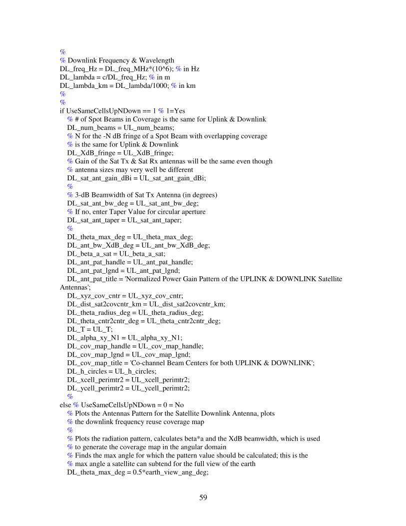
59

% % Downlink Frequency & Wavelength DL_freq_Hz = DL_freq_MHz*(10^6); % in Hz DL_lambda = c/DL_freq_Hz; % in m DL_lambda_km = DL_lambda/1000; % in km % % if UseSameCellsUpNDown == 1 % 1=Yes % # of Spot Beams in Coverage is the same for Uplink & Downlink DL_num_beams = UL_num_beams; % N for the -N dB fringe of a Spot Beam with overlapping coverage % is the same for Uplink & Downlink DL_XdB_fringe = UL_XdB_fringe; % Gain of the Sat Tx & Sat Rx antennas will be the same even though % antenna sizes may very well be different DL_sat_ant_gain_dBi = UL_sat_ant_gain_dBi; % % 3-dB Beamwidth of Sat Tx Antenna (in degrees) DL_sat_ant_bw_deg = UL_sat_ant_bw_deg; % If no, enter Taper Value for circular aperture DL_sat_ant_taper = UL_sat_ant_taper; % DL_theta_max_deg = UL_theta_max_deg; DL_ant_bw_XdB_deg = UL_ant_bw_XdB_deg; DL_beta_a_sat = UL_beta_a_sat; DL_ant_pat_handle = UL_ant_pat_handle; DL_ant_pat_lgnd = UL_ant_pat_lgnd; DL_ant_pat_title = 'Normalized Power Gain Pattern of the UPLINK & DOWNLINK Satellite Antennas'; DL_xyz_cov_cntr = UL_xyz_cov_cntr; DL_dist_sat2covcntr_km = UL_dist_sat2covcntr_km; DL_theta_radius_deg = UL_theta_radius_deg; DL_theta_cntr2cntr_deg = UL_theta_cntr2cntr_deg; DL_T = UL_T; DL_alpha_xy_N1 = UL_alpha_xy_N1; DL_cov_map_handle = UL_cov_map_handle; DL_cov_map_lgnd = UL_cov_map_lgnd; DL_cov_map_title = 'Co-channel Beam Centers for both UPLINK & DOWNLINK'; DL_h_circles = UL_h_circles; DL_xcell_perimtr2 = UL_xcell_perimtr2; DL_ycell_perimtr2 = UL_ycell_perimtr2; % else % UseSameCellsUpNDown = 0 = No % Plots the Antennas Pattern for the Satellite Downlink Antenna, plots % the downlink frequency reuse coverage map % % Plots the radiation pattern, calculates beta*a and the XdB beamwidth, which is used % to generate the coverage map in the angular domain % Finds the max angle for which the pattern value should be calculated; this is the % max angle a satellite can subtend for the full view of the earth DL_theta_max_deg = 0.5*earth_view_ang_deg;

60

if DL_sat_ant_bw_deg > earth_view_ang_deg DL_sat_ant_bw_deg = earth_view_ang_deg; end [DL_ant_bw_XdB_deg, DL_beta_a_sat, DL_ant_pat_handle] = plot_ant_pattern(DL_sat_ant_taper, ... DL_XdB_fringe, DL_sat_ant_bw_deg, DL_theta_max_deg); DL_ant_pat_lgnd = 'Pattern Data'; DL_ant_pat_title = 'Normalized Power Gain Pattern of the DOWNLINK Satellite Antenna'; title(DL_ant_pat_title); % % Plots the coverage map on a plane where (x,y) positions actually correspond to % angles, and so, the distance between any point and the origin is the angle that % cell center makes with the line joining the satellite & the center of coverage. % % Converting Lat/Long to cartesian coordinates for use later DL_xyz_cov_cntr = lat2xyz(DL_cov_cntr_lat_deg, DL_cov_cntr_long_deg, 0); % % Coverage Center Visibility Test DL_cov_cntr_lat_rad = DL_cov_cntr_lat_deg*pi/180; DL_cov_cntr_long_rad = DL_cov_cntr_long_deg*pi/180; sat_lat_rad = sat_lat_deg*pi/180; sat_long_rad = sat_long_deg*pi/180; [DL_dist_sat2covcntr_km, isvisib] = visibNelev_test(DL_cov_cntr_lat_rad, ... DL_cov_cntr_long_rad); % [DL_alpha_xy_N1, DL_cell_ang_dist_mtx, DL_T, DL_cov_map_handle] = plot_coverage_map... (xyz_sat, xyz_subsat, DL_xyz_cov_cntr, DL_num_beams, DL_reuse_num, DL_ant_bw_XdB_deg); % DL_cov_map_lgnd = 'Beam Center'; DL_cov_map_title = 'Co-channel Beam Centers for the DOWNLINK'; title(DL_cov_map_title); xlabel('Alpha y-axis (degrees)'); ylabel('Alpha x-axis (degrees)'); % DL_theta_radius_deg = DL_cell_ang_dist_mtx(1,1); DL_theta_cntr2cntr_deg = DL_cell_ang_dist_mtx(2,1); DL_theta_cochannel_deg = DL_cell_ang_dist_mtx(3,1); % % Draws the circular beam perimeter (in angular domain) around the cell centers % This code is placed here so that the legend labels aren't needed for these circles DL_theta = -0.01:0.01:2*pi; DL_r = DL_theta_radius_deg*ones(1,length(DL_theta)); [DL_ycell_perimtr, DL_xcell_perimtr] = pol2cart(DL_theta, DL_r); DL_x_y_cntrs = [DL_alpha_xy_N1(:,1), DL_alpha_xy_N1(:,2)]; for DL_cell_no = 1:size(DL_x_y_cntrs,1) DL_xcell_perimtr2(DL_cell_no,:) = DL_xcell_perimtr + DL_x_y_cntrs(DL_cell_no,1); DL_ycell_perimtr2(DL_cell_no,:) = DL_ycell_perimtr + DL_x_y_cntrs(DL_cell_no,2); end figure(DL_cov_map_handle)

61

hold on DL_h_circles = plot(DL_ycell_perimtr2', DL_xcell_perimtr2', 'b'); end % if DL_es_loc == 0 % 0 is to specify Lat/Long for ES location % Conversion to units that are more useful DL_es_lat_rad = DL_es_lat_deg*pi/180; % in radians DL_es_long_rad = DL_es_long_deg*pi/180; % in radians % [DL_dist_sat2es_km, isvisib] = visibNelev_test(DL_es_lat_rad, DL_es_long_rad) % Uses a custom function 'lat2xyz' to convert Lat/Long to XYZ DL_xyz_es = lat2xyz(DL_es_lat_deg, DL_es_long_deg, 0); % % Projects the user location to the alpha_xy coordinate system using % the custom function 'proj2alpha_xy'; this also checks to make sure % that the ES falls within the defined coverage radius [DL_alpha_xy_escellcntr, DL_alpha_xy_es, IsDLesInCoverage] = ... proj2alpha_xy(xyz_sat, DL_xyz_es, DL_xyz_cov_cntr, DL_alpha_xy_N1,... DL_T, DL_theta_radius_deg); hold on plot(DL_alpha_xy_es(2), DL_alpha_xy_es(1), 'hk', 'MarkerSize', 10.5); DL_cov_map_lgnd = strvcat(DL_cov_map_lgnd, 'Downlink User') % % Angle between ES and ES-cell's center; to be used to calculate % f_theta_es later DL_ang_es2escellcntr_deg = ... sqrt((DL_alpha_xy_escellcntr(:,2) - DL_alpha_xy_es(2)).^2 + ... (DL_alpha_xy_escellcntr(:,1) - DL_alpha_xy_es(1)).^2); % if IsDLesInCoverage == 0 error(' The user is not in the coverage area'); end else % DL_es_loc == 1 is to select the ES location on the coverage map % Getting location info for the Downlink Earth Station figure(DL_cov_map_handle); DL_h_msgBox= msgbox(... 'Click on the desired location of the DOWNLINK Earth Station.',... 'Figure Input Dialog Box'); uiwait(DL_h_msgBox) uiresume(DL_cov_map_handle) %figure(DL_cov_map_handle); DL_alpha_xy_es_input = ginput(1); % in degrees % Swap X & Y to match the norm in Figure 1 DL_alpha_xy_es = [DL_alpha_xy_es_input(2) DL_alpha_xy_es_input(1)]; hold on DL_h_ini_user_loc = plot(DL_alpha_xy_es(2), DL_alpha_xy_es(1), '+k'); % Find coverage cell center closest to this point NOT greater than 0.5*bw DL_ang_es2cellcntrs_deg = sqrt((DL_alpha_xy_N1(:,2) - DL_alpha_xy_es(2)).^2 +... (DL_alpha_xy_N1(:,1) - DL_alpha_xy_es(1)).^2); [DL_ang_es2cellcntrs_min_deg, min_index] = min(DL_ang_es2cellcntrs_deg); if DL_ang_es2cellcntrs_min_deg > (0.5*DL_ant_bw_XdB_deg)

62

disp(' ') error(' The selected user location is outside the closest coverage cell') disp(' ') else DL_alpha_xy_escellcntr = DL_alpha_xy_N1(min_index, 1:2); end % Finds Theta & Rho for the user input with 'DL_alpha_xy_escellcntr' as % origin; this makes it simpler to place user at desired location in cell DL_alpha_xy_es_wrt_escellcntr = DL_alpha_xy_es - DL_alpha_xy_escellcntr; % Convert cartesian to polar % [TH,R] = CART2POL(X,Y) [DL_theta_es_wrt_escellcntr_rad, DL_rho_es_wrt_escellcntr_deg] =... cart2pol(DL_alpha_xy_es_wrt_escellcntr(2), DL_alpha_xy_es_wrt_escellcntr(1)); % % Location Pt. on Spot Beam (0=Center; 1=Mid-Pt.; 2=Fringe) if DL_es_loc_on_spot_beam == 0 % User location at cell center DL_theta_es_wrt_escellcntr_rad = 0; DL_rho_es_wrt_escellcntr_deg = 0; end if DL_es_loc_on_spot_beam == 1 % mid-pt between fringe & center of cell DL_rho_es_wrt_escellcntr_deg = 0.25*DL_ant_bw_XdB_deg; end if DL_es_loc_on_spot_beam == 2 % at the fringe if size(DL_alpha_xy_N1,1) == 1 DL_rho_es_wrt_escellcntr_deg = 0.5*DL_ant_bw_XdB_deg; else % This is done so that the user doesn't land up in the adjacent cell DL_rho_es_wrt_escellcntr_deg = 0.5*DL_theta_cntr2cntr_deg; end end % Convert this back to Cartesian w.r.t. coverage center as origin % [X,Y] = pol2cart(THETA,RHO) [DL_alpha_xy_es_wrt_escellcntr(2), DL_alpha_xy_es_wrt_escellcntr(1)] = pol2cart... (DL_theta_es_wrt_escellcntr_rad, DL_rho_es_wrt_escellcntr_deg); DL_alpha_xy_es = DL_alpha_xy_es_wrt_escellcntr + DL_alpha_xy_escellcntr; delete(DL_h_ini_user_loc) plot(DL_alpha_xy_es(2), DL_alpha_xy_es(1), 'hk', 'MarkerSize', 10.5); DL_cov_map_lgnd = strvcat(DL_cov_map_lgnd, 'Downlink User') % Angle between ES and ES-cell's center; to be used to calculate % f_theta_es later DL_ang_es2escellcntr_deg = DL_rho_es_wrt_escellcntr_deg; end % % Finds the path loss for the user (it's the same for the DL interfering beams). % Calculates the distance between the Satellite and the ES DL_earth_center_xpypzp = DL_T*([0;0;0]-xyz_sat); DL_dist_sat2es_km = dist_sat2earth(DL_alpha_xy_es, DL_earth_center_xpypzp); % The Path Loss formula DL_path_loss_es = 4*pi*DL_dist_sat2es_km/DL_lambda_km; DL_path_loss_es_dB = 20*log10(DL_path_loss_es) % used for verification %

63

if IsReuseUsed4Downlink == 0 % 0=No, 1=Yes % Then no co-channel inerferers exist, but the CNR can still be calculated % % Since there is no reuse, the angle between the ES cell center and the % coverage center is 0; which implies that there is no scan loss DL_num_co_ch_tiers_used = 0; DL_num_co_ch_tiers_in_cov = 0; DL_num_co_ch_cells = 0; DL_ang_escellcntr2covcntr_deg = 0; % Scan Loss (in dB) = 10*k*log[cos(theta)] DL_scan_loss_dB = -10*DL_scan_loss_k*log10(cos(DL_ang_escellcntr2covcntr_deg*pi/180)); else % if Reuse is used for the Downlink % Calculates the angles between co-channel cell centers and the user % DL_alpha_xy_CCC(:, 5) are the angles between co-channel cell centers & user cell center % DL_alpha_xy_CCC(:, 6) are the angles between co-channel cell centers & actual user location DL_alpha_xy_CCC = co_ch_ang_mtx('DOWNLINK', DL_alpha_xy_N1, DL_num_beams, DL_reuse_num, DL_alpha_xy_es,... DL_alpha_xy_escellcntr, DL_theta_cntr2cntr_deg, UseSameCellsUpNDown); % Only uses the number of co-channel tiers that are desired if DL_tiers2use == 100 DL_tiers2use = max(DL_alpha_xy_CCC(:,3)); % First entry is that of the cell center where the ES is, so: DL_alpha_xy_CCC2use = DL_alpha_xy_CCC(2:end,:); else DL_tiers2use = 1; DL_alpha_xy_CCC2use = DL_alpha_xy_CCC(DL_alpha_xy_CCC(:,3)==DL_tiers2use, :); end DL_num_co_ch_tiers_used = DL_tiers2use; DL_num_co_ch_tiers_in_cov = max(DL_alpha_xy_CCC(:,3)); % figure(DL_cov_map_handle) hold on plot(DL_alpha_xy_CCC(1,2), DL_alpha_xy_CCC(1,1), 'dk', ... DL_alpha_xy_CCC2use(:,2), DL_alpha_xy_CCC2use(:,1), 'vk', 'MarkerSize', 10.5); % DL_cov_map_lgnd = strvcat(DL_cov_map_lgnd, 'Downlink Usercell', 'Downlink Co-Ch Cells'); % Angle between the ES-cell's center & the center of coverage DL_ang_escellcntr2covcntr_deg = sqrt((DL_alpha_xy_CCC(1,1))^2 + (DL_alpha_xy_CCC(1,2))^2); % Angle between ES and ES-cell's center; to be used to calculate % f_theta_es later DL_ang_es2escellcntr_deg = DL_alpha_xy_CCC(1, 6) % Angle between the ES & the center of coverage DL_ang_es2covcntr_deg = sqrt((DL_alpha_xy_es(1,1))^2 + (DL_alpha_xy_es(1,2))^2); % % Assume that there's exactly one active interferer in each of % the interfering co-channel cells. % Total number of co-channel cell interferers

64

DL_num_co_ch_cells = size(DL_alpha_xy_CCC2use,1) % % Calculation for Interference power received by the downlink user DL_f_theta = pattern_value(DL_sat_ant_taper, DL_alpha_xy_CCC2use(:,6), DL_beta_a_sat); DL_f_theta_dB = 20*log10(DL_f_theta); % % Plots the angles for the interfering beams on the Satellite Antenna Pattern Plot figure(DL_ant_pat_handle) hold on plot(DL_alpha_xy_CCC2use(:,6), DL_f_theta_dB, 'pk', 'MarkerSize', 10); DL_intf_max_ang = max(DL_alpha_xy_CCC2use(:,6)); DL_ant_pat_lgnd = strvcat(DL_ant_pat_lgnd, 'Downlink Intfs') % % Scan Loss for the different interfering beams = [cos(theta)]^k DL_intf_scan_loss = (cos(DL_alpha_xy_CCC2use(:,6).*pi/180)).^DL_scan_loss_k; % Sum of Interference powers in dB = other values + 20log[sum(f_theta/dist2earth)] % Puts the f_theta & distance values together in a matrix fNscanloss = [DL_f_theta.^2, DL_intf_scan_loss]; fNscanloss(:,3) = [(fNscanloss(:,1)./fNscanloss(:,2))]; DL_fNscanloss_sum = sum(fNscanloss(:,3)); DL_fNscanloss_sum_dB = 10*log10(DL_fNscanloss_sum); % DL_intf_pwr_dBW = DL_sat_tx_pwr_dBW + DL_sat_tx_bo_dBW + DL_sat_ant_gain_dBi... + DL_es_ant_gain_dBi + DL_fNscanloss_sum_dB - DL_atm_loss_dB... - DL_misc_loss_dB - DL_path_loss_es_dB; DL_intf_pwr = 10^(DL_intf_pwr_dBW/10); end % % Shows legends for the Antenna Pattern Plot figure(DL_ant_pat_handle) title(DL_ant_pat_title) legend(DL_ant_pat_lgnd, 1); legend('boxoff') % Deletes the circle boundaries so that legend labels can be easily applied figure(DL_cov_map_handle) hold on title(DL_cov_map_title) delete(DL_h_circles) % Shows legends for the Coverage Map legend(DL_cov_map_lgnd, -1); % Shows the circle boundaries again plot(DL_ycell_perimtr2', DL_xcell_perimtr2', 'b'); axis equal % Scan Loss (in dB) = 10*k*log[cos(theta)] DL_es_scan_loss_dB = -10*DL_scan_loss_k*log10(cos(DL_ang_escellcntr2covcntr_deg*pi/180)); % % Calculates the satellite antenna gain pattern value to be used % since the ES may not be at the center of the ES-cell if DL_ang_es2escellcntr_deg == 0 DL_f_theta_es = 1;

65

else DL_f_theta_es = pattern_value(DL_sat_ant_taper, DL_ang_es2escellcntr_deg, DL_beta_a_sat); end DL_f_theta_es_dB = 20*log10(DL_f_theta_es) % used for verification % % Carrier power received by the Satellite Receiver DL_C_pwr_dBW = DL_sat_tx_pwr_dBW + DL_sat_tx_bo_dBW + DL_sat_ant_gain_dBi... + DL_es_ant_gain_dBi + DL_f_theta_es_dB - DL_path_loss_es_dB ... - DL_atm_loss_dB - DL_misc_loss_dB - DL_misc_loss_es_dB - DL_es_scan_loss_dB; DL_C_pwr = 10^(DL_C_pwr_dBW/10); % in Watts % %% CALCULATION FOR NOISE POWER DL_Noise_pwr_dBW = ktb_dBW(DL_SysNoiseTemp_K, DL_NoiseBW_kHz) DL_Noise_pwr = 10^(DL_Noise_pwr_dBW/10); % in Watts % %% CALCULATIONS FOR CARRIER TO NOISE RATIO (CNR) DL_CNR_dB = DL_C_pwr_dBW - DL_Noise_pwr_dBW DL_CNR = 10^(DL_CNR_dB/10); % %% CALCULATIONS FOR CARRIER TO NOISE + INTERFERENCE RATIO (CNIR) if IsReuseUsed4Downlink == 1 % 0=No, 1=Yes DL_CIR_dB = DL_C_pwr_dBW - DL_intf_pwr_dBW; DL_CIR = 10^(DL_CIR_dB/10); else DL_CIR = inf; DL_CIR_dB = 10*log10(DL_CIR); DL_intf_pwr = 0; end DL_CNIR = 1/(1/DL_CNR + 1/DL_CIR); DL_CNIR_dB = 10*log10(DL_CNIR); DL_CNIR_test = DL_C_pwr/(DL_Noise_pwr + DL_intf_pwr); DL_CNIR_dB_test = 10*log10(DL_CNIR_test); % % %%%%%%%%%%%%%%%%%%%%%%%%%%%%%%%%%%%%%%%%%%%%%%% % CALCULATIONS FOR DEGRADATION IN OVERALL C/N % %%%%%%%%%%%%%%%%%%%%%%%%%%%%%%%%%%%%%%%%%%%%%%% % DL_degrdtn2CNR_dB = round(100*(DL_CNR_dB - DL_CNIR_dB))/100; % UL_degrdtn2CNR_WC_dB = round(100*(UL_CNR_dB - UL_CNIR_WC_dB))/100; UL_degrdtn2CNR_BC_dB = round(100*(UL_CNR_dB - UL_CNIR_BC_dB))/100; UL_degrdtn2CNR_rdm_dB = round(100*(UL_CNR_dB - UL_CNIR_rdm_dB))/100; % CNIR_WC_overall = 1/(1/UL_CNIR_WC + 1/DL_CNIR); CNIR_WC_overall_dB = round(100*(10*log10(CNIR_WC_overall)))/100; % CNIR_BC_overall = 1/(1/UL_CNIR_BC + 1/DL_CNIR); CNIR_BC_overall_dB = round(100*(10*log10(CNIR_BC_overall)))/100; %

66

CNIR_rdm_overall = 1/(1/UL_CNIR_rdm + 1/DL_CNIR); CNIR_rdm_overall_dB = round(100*(10*log10(CNIR_rdm_overall)))/100; % CNR_overall = 1/(1/UL_CNR + 1/DL_CNR); CNR_overall_dB = round(100*(10*log10(CNR_overall)))/100; degrdtn2CNR_overall_rdm_dB = round(100*(CNR_overall_dB - CNIR_rdm_overall_dB))/100; degrdtn2CNR_overall_WC_dB = round(100*(CNR_overall_dB - CNIR_WC_overall_dB))/100; degrdtn2CNR_overall_BC_dB = round(100*(CNR_overall_dB - CNIR_BC_overall_dB))/100; % %%%%%%%%%%%%%%%%%%%%%%%%%%%%%%%%%%%%%%%%%%%%% % Displays Ouput Data in the Command Window % %%%%%%%%%%%%%%%%%%%%%%%%%%%%%%%%%%%%%%%%%%%%% % disp(' ') disp(' ================') disp(' WANTED RESULTS') disp(' ================') % format compact format short g disp(' ') disp('======= DOWNLINK ========') DL_reuse_num DL_num_co_ch_tiers_used DL_num_co_ch_tiers_in_cov DL_num_co_ch_cells DL_sat_ant_taper DL_f_theta_es_dB DL_CNR_dB DL_CIR_dB DL_CNIR_dB DL_degrdtn2CNR_dB disp(' ') disp('======= UPLINK ========') UL_reuse_num UL_num_co_ch_tiers_used UL_num_co_ch_tiers_in_cov UL_num_co_ch_cells UL_sat_ant_taper UL_f_theta_es_dB UL_CNR_dB UL_CIR_WC_dB UL_CIR_BC_dB UL_CIR_rdm_dB UL_CNIR_rdm_dB UL_CNIR_WC_dB UL_CNIR_BC_dB disp(' ') disp('======= OVERALL ========') earth_view_ang_deg DL_reuse_num

67

UL_reuse_num DL_sat_ant_taper UL_sat_ant_taper DL_num_beams UL_num_beams DL_tiers2use UL_tiers2use CNR_overall_dB CNIR_WC_overall_dB CNIR_BC_overall_dB CNIR_rdm_overall_dB degrdtn2CNR_overall_rdm_dB degrdtn2CNR_overall_WC_dB degrdtn2CNR_overall_BC_dB disp(' ') % disp(' ================') disp(' END OF PROGRAM') disp(' ================')

68

Appendix C

User-Defined Functions Called by the Main Computer Code

This appendix presents the supporting functions for the main computer code.

function xyz = lat2xyz(Lat, Long, h) % xyz = lat2xyz(Lat, Long, h) assumes that the earth is spherical % in shape. It converts the more common Lat & Long coordinates % to the cartesian coordinates by first calculating the spherical % coordinates Phi(angle from the z-axis) and Theta (angle from % the x-axis). This also assumes that the Theta = 0 plane passes % through the Greenwich Meridian for which Longitude = 0, and % +ve y-axis is east of this plane. % % Text Updated 7/31/06 % Code Updated 6/24/05 global earth_radius %% For Independent testing %Lat = 35.25; % degrees %Long = 120.5; % degrees %Re = 6378.137; % km %% % Latitude values range from 90deg (North pole) to -90deg (South pole) % and Phi is measured from the +ve z-axis; range: 0-180 deg Phi = 90 - Lat; % in degrees % Longitude values range from 0deg (Greenwich Meridian) to 360deg West % and Theta is measured from the +ve x-axis; range: -180 to 180 degrees % positive angle towards the +ve y-axis or towards East Theta = -Long; % in degrees R = h + earth_radius; % same unit as earth radius % Relationships between Spherical & Cartesian x = R*sin(Phi*pi/180)*cos(Theta*pi/180); % same unit as earth radius y = R*sin(Phi*pi/180)*sin(Theta*pi/180); % same unit as earth radius z = R*cos(Phi*pi/180); % same unit as earth radius xyz = [x;y;z]; % % END OF FUNCTION

69

function [ant_bw_XdB_deg, beta_a, plot_handle] = plot_ant_pattern(taper, ... XdB_fringe, ant_bw_deg, theta_max_deg) %[ant_bw_XdB_deg, beta_a, plot_handle] = plot_ant_pattern(taper, ... % XdB_fringe, ant_bw_deg, theta_max_deg) % % It calculates 'beta*a' for the given parameters and plots the normalized % gain pattern for a Uniformly/Taper-Illuminated Circular Pattern. % It also calculates the XdB beamwidth in degrees of the antenna, given % its 3-dB beamwidth, 'ant_bw_deg'. % % Updated July 31, 2006 %% For testing only %taper = 0; %XdB_fringe = 4; %ant_bw_deg = 1; %theta_max_deg = 5; % Plot of radiation pattern: % f(theta)=abs[2*J{beta*a*sin(theta)}/{beta*a*sin(theta)}] % Calculate the value of f(theta) for the 3dB value dB_value = 10*log10(2); % is a precise way to put 3dB f_3dB_value = 10^(-dB_value/20); % not a dB value % Finds t = beta*a*sin(theta) for which f(theta) = f_xdB t = 0.1:0.1:10; % unitless f_t = abs((2.^(taper+1)).*factorial(taper+1).*besselj(taper+1, t)./... (t.^(taper+1))); t_3dB_value = interp1(f_t, t, f_3dB_value,'spline'); % Finds 'beta*a' using: % beta*a*sin(theta(3dB_value)) = t_3dB_value % also, theta(3dB_value) = 0.5*sat_ant_bw_deg beta_a = t_3dB_value/sin(0.5*ant_bw_deg*pi/180); % unitless quantity % beta_a = 16.55; theta_ini = 0.0010; step = 0.0001; theta_axis_limit = 1.0*theta_max_deg; theta = theta_ini:step:theta_axis_limit*pi/180; arg = beta_a.*sin(theta); f_theta = abs((2^(taper+1))*factorial(taper+1).*besselj(taper+1, arg)./... (arg.^(taper+1))); f_theta_dB = 20.*log10(f_theta); % Finds the value of theta for which f(theta) = -XdB theta_XdB = interp1(f_theta_dB, theta, -XdB_fringe,'spline'); ant_bw_XdB_deg = 2*theta_XdB*180/pi; figure % Saves the current figure's handle for later use plot_handle = get(0,'CurrentFigure'); % Plots the normalized antenna pattern plot(theta*180/pi, f_theta_dB) axis([0 theta_axis_limit -100 5]) % END OF FUNCTION

70

function [path_length_km, isvisib] = visibNelev_test(lat_rad, long_rad) % [path_length_km, isvisib] = visibNelev_test(lat_rad, long_rad) % Finds out whether the Satellite is visible from 'lat/long' and % if the elevation angle of the Satellite is greater than 'minElev'. % % Text Updated 7/31/06 % Code Updated 8/02/06 global earth_radius sat_ht_abv_earth sat_lat_deg sat_long_deg minElev %% For independent testing only %format short g %earth_radius = 6378.137; % in km %lat_rad = 52*pi/180; %long_rad = 0; %sat_lat_rad = 0; %sat_long_rad = 66*pi/180; %sat_ht_abv_earth = 35786.033; % in km %minElev = 10; %% % % Calculations for path length & satellite visibility test sat_lat_rad = sat_lat_deg*pi/180; sat_long_rad = sat_long_deg*pi/180; isvisib = 'YES'; % default value cos_gamma = cos(lat_rad)*cos(sat_lat_rad)*cos(sat_long_rad ... -long_rad) + sin(lat_rad)*sin(sat_lat_rad); gamma = acos(cos_gamma); gamma_deg = gamma*180/pi; % in deg sat2earthcenter = sat_ht_abv_earth + earth_radius; % in km % Formula for path length has been taken from (34, Pratt2003) path_length_km = sat2earthcenter*sqrt(1 + (earth_radius/sat2earthcenter)^2 ... - 2*(earth_radius/sat2earthcenter)*cos_gamma) path_length = path_length_km*1000; % in meters % Test Variable test_var = earth_radius/cos_gamma; % in km % % gamma should not be greater than 81.3 degrees for a satellite % to be visible assuming that no satellite/platform will be placed % further than a GEO satellite's orbital radius of 42,164.17 km. % Visibility Test taken from (36, Pratt2003) if (sat2earthcenter < test_var) | (gamma_deg >81.3) disp(' ') isvisib = 'NO' error('The Satellite/Platform is not in line-of-sight'); disp(' ') end % % Elevation calculation, taken from (34, Pratt2003) elevation = 180/pi*acos(sat2earthcenter*sin(gamma)/path_length_km) % in deg

71

if elevation < minElev disp(' ') error(sprintf('Elevation angle less than %g is not permitted', minElev)); disp(' ') end % gamma_deg path_length_km isvisib % % END OF FUNCTION

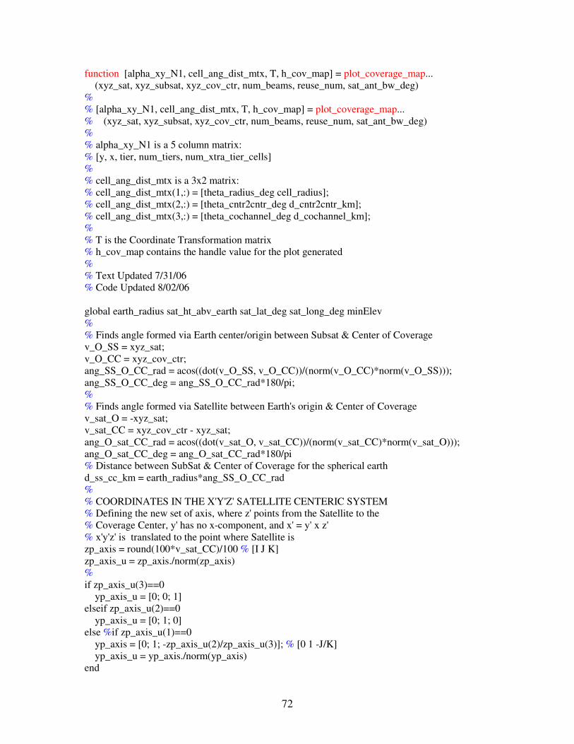
72

function [alpha_xy_N1, cell_ang_dist_mtx, T, h_cov_map] = plot_coverage_map... (xyz_sat, xyz_subsat, xyz_cov_ctr, num_beams, reuse_num, sat_ant_bw_deg) % % [alpha_xy_N1, cell_ang_dist_mtx, T, h_cov_map] = plot_coverage_map... % (xyz_sat, xyz_subsat, xyz_cov_ctr, num_beams, reuse_num, sat_ant_bw_deg) % % alpha_xy_N1 is a 5 column matrix: % [y, x, tier, num_tiers, num_xtra_tier_cells] % % cell_ang_dist_mtx is a 3x2 matrix: % cell_ang_dist_mtx(1,:) = [theta_radius_deg cell_radius]; % cell_ang_dist_mtx(2,:) = [theta_cntr2cntr_deg d_cntr2cntr_km]; % cell_ang_dist_mtx(3,:) = [theta_cochannel_deg d_cochannel_km]; % % T is the Coordinate Transformation matrix % h_cov_map contains the handle value for the plot generated % % Text Updated 7/31/06 % Code Updated 8/02/06 global earth_radius sat_ht_abv_earth sat_lat_deg sat_long_deg minElev % % Finds angle formed via Earth center/origin between Subsat & Center of Coverage v_O_SS = xyz_sat; v_O_CC = xyz_cov_ctr; ang_SS_O_CC_rad = acos((dot(v_O_SS, v_O_CC))/(norm(v_O_CC)*norm(v_O_SS))); ang_SS_O_CC_deg = ang_SS_O_CC_rad*180/pi; % % Finds angle formed via Satellite between Earth's origin & Center of Coverage v_sat_O = -xyz_sat; v_sat_CC = xyz_cov_ctr - xyz_sat; ang_O_sat_CC_rad = acos((dot(v_sat_O, v_sat_CC))/(norm(v_sat_CC)*norm(v_sat_O))); ang_O_sat_CC_deg = ang_O_sat_CC_rad*180/pi % Distance between SubSat & Center of Coverage for the spherical earth d_ss_cc_km = earth_radius*ang_SS_O_CC_rad % % COORDINATES IN THE X'Y'Z' SATELLITE CENTERIC SYSTEM % Defining the new set of axis, where z' points from the Satellite to the % Coverage Center, y' has no x-component, and x' = y' x z' % x'y'z' is translated to the point where Satellite is zp_axis = round(100*v_sat_CC)/100 % [I J K] zp_axis_u = zp_axis./norm(zp_axis) % if zp_axis_u(3)==0 yp_axis_u = [0; 0; 1] elseif zp_axis_u(2)==0 yp_axis_u = [0; 1; 0] else %if zp_axis_u(1)==0 yp_axis = [0; 1; -zp_axis_u(2)/zp_axis_u(3)]; % [0 1 -J/K] yp_axis_u = yp_axis./norm(yp_axis) end

73

% xp_axis_u = cross(yp_axis_u, zp_axis_u) % y' x z' % zp_axis_u2 = round(cross(xp_axis_u, yp_axis_u).*1000)/1000 % for testing only % % Transformation matrix to go from XYZ to X'Y'Z' system T = vertcat(xp_axis_u', yp_axis_u', zp_axis_u') Tinv = inv(T) % %% test to see if Tinv & T-transposed are the same Ttxp = T' % % GENERATION OF COVERAGE MAP % % Total number of complete Clusters used for coverage num_clusters = floor(num_beams/reuse_num); % % Coverage cell diameter assuming a spherical Earth % The cell radius below is only for a cell lying on the sub/sat-pt. sat_ant_bw_rad = sat_ant_bw_deg*pi/180; cell_radius = arc_length(earth_radius, sat_ht_abv_earth, sat_ant_bw_rad) % in km cell_diamtr = 2*cell_radius; % in km % %% Verifies beamwidth % Angle formed at the origin/earth's center theta_radius_E_rad = cell_radius/earth_radius; % Angle formed at the Satellite % Equation 10.3 from Figure 10 of the notes theta_radius_S_rad = atan(earth_radius*sin(theta_radius_E_rad)/... (sat_ht_abv_earth + earth_radius*(1 - cos(theta_radius_E_rad)))); theta_radius_S_deg = theta_radius_S_rad*180/pi % Beamwidth of the Satellite Antenna theta_bw = round(100*2*theta_radius_S_deg)/100 %% % Cell radius in degrees theta_radius_deg = sat_ant_bw_deg/2; % Calculates the angle between a cell-center and an adjacent cell-center % This is true only for cells at the sub-sat pt.; but it's also used for % any two cells in coverage. theta_cntr2cntr_deg = theta_radius_deg * sqrt(3); % in deg % % Dist(center2center) = 2 x cell_radius x cos(30deg) = r x SQRT(3) d_cntr2cntr_km = 2 * cell_radius * cos(pi/6); % in km % % Angle between a cell and a co-channel cell; at the sub/sat-pt. % = cell_radius * sqrt(3*Reuse_number) theta_cochannel_deg = theta_radius_deg * sqrt(3*reuse_num); % in deg % d_cochannel_km = cell_radius * sqrt(3*reuse_num); % in km % % A 2-D planar coverage map is used to specify beam centers that, in

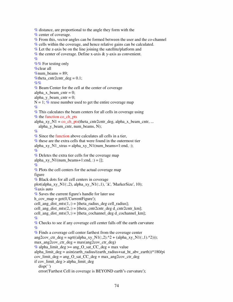
74

% distance, are proportional to the angle they form with the % center of coverage. % From this, vector angles can be formed between the user and the co-channel % cells within the coverage, and hence relative gains can be calculated. % Let the z-axis be on the line joining the satellite/platform and % the center of coverage. Define x-axis & y-axis as convenient. % %% For testing only %clear all %num_beams = 89; %theta_cntr2cntr_deg = 0.1; %% % Beam Center for the cell at the center of coverage alpha_x_beam_cntr = 0; alpha_y_beam_cntr = 0; N = 1; % reuse number used to get the entire coverage map % % This calculates the beam centers for all cells in coverage using % the function co_ch_pts alpha_xy_N1 = co_ch_pts(theta_cntr2cntr_deg, alpha_x_beam_cntr, ... alpha_y_beam_cntr, num_beams, N); % % Since the function above calculates all cells in a tier, % these are the extra cells that were found in the outermost tier alpha_xy_N1_xtras = alpha_xy_N1(num_beams+1:end, :); % % Deletes the extra tier cells for the coverage map alpha_xy_N1(num_beams+1:end, :) = []; % % Plots the cell centers for the actual coverage map figure % Black dots for all cell centers in coverage plot(alpha_xy_N1(:,2), alpha_xy_N1(:,1), '.k', 'MarkerSize', 10); %axis auto % Saves the current figure's handle for later use h_cov_map = get(0,'CurrentFigure'); cell_ang_dist_mtx(1,:) = [theta_radius_deg cell_radius]; cell_ang_dist_mtx(2,:) = [theta_cntr2cntr_deg d_cntr2cntr_km]; cell_ang_dist_mtx(3,:) = [theta_cochannel_deg d_cochannel_km]; % % Checks to see if any coverage cell center falls off the earth curvature % % Finds a coverage cell center farthest from the coverage center ang2cov_ctr_deg = sqrt((alpha_xy_N1(:,2).^2 + (alpha_xy_N1(:,1).^2))); max_ang2cov_ctr_deg = max(ang2cov_ctr_deg) % alpha_limit_deg >= ang_O_sat_CC_deg + max value alpha_limit_deg = asin(earth_radius/(earth_radius+sat_ht_abv_earth))*180/pi cov_limit_deg = ang_O_sat_CC_deg + max_ang2cov_ctr_deg if cov_limit_deg > alpha_limit_deg disp(' ') error('Farthest Cell in coverage is BEYOND earth''s curvature');

75

disp(' ') end % % END OF FUNCTION

76

function r_ans = arc_length(Re, h, theta_bw_rad) % r_ans = arc_length(Re, h, theta_bw_rad) % Graphical method of determining the cell-radius/arc-length 'r' % Given: Earth Radius, Height of Space Station above Earth, and % Beamwidth in radians. % Calculated 'r' is in the same units as distances given above. % % Updated April 4, 2006 % Refer to Figure 9B of the notes % %Re = 6400; % Earth Radius in km %h = 12000; % height of satellite in km %theta_bw = 1*pi/180; % beam-width in radians % r_est is an estimate for cell-radius by using the s = r.theta r_est = h * theta_bw_rad/2; % Estimate the region for the actual value of r_est r = r_est/2:0.001:2*r_est; % changed from 0.0001 resolution for lower MEMORY use % Formula derived from Figure 9B of notes y = sin(r./Re) + tan(theta_bw_rad/2)*cos(r./Re) - ((Re + h)/Re*tan(theta_bw_rad/2)); %plot(y) y_mag = abs(y); [y_ans,index] = min(y_mag); %y_ans = y(index) r_ans = r(index);

77

function x_y_cntr = co_ch_pts(theta_deg, x_cntr, y_cntr, num_beams, N) % CALCULATES THE MAXIMUM-GAIN ANGLES ON AN X-Y PLANE % % x_y_cntr = co_ch_pts(theta_deg, x_cntr, y_cntr, N) % % x_y_cntr: is a 5 column matrix: [y x tier num_tiers num_xtra_tier_cells] % theta_deg: is the angle in degrees between any two adjacent cells % x_cntr, y_cntr: are the coordinates for the beam around which co-channel % cells have to be identified % N: is the cell reuse number % If N=1, all beam centers in coverage are calculated; % If N=3, all co-channel beam centers are calculated % % updated 3/23/06 % %% FOR INDEPENDENT TESTING %clear all %num_beams = 89; %i=1; %j=0; %theta_deg = 0.1; %x_cntr = 0; %y_cntr = 0; %N = 4; %% %global num_beams i_mtx = 1:10; j_mtx(i_mtx) = (-i_mtx + sqrt(i_mtx.^2 - 4*(i_mtx.^2 - N)))/2; % This finds the index of only real values in J_MTX index_real_j_mtx = find(angle(j_mtx)==0); % finds the whole numbers in J_MTX jdiff = j_mtx(index_real_j_mtx) - round(j_mtx(index_real_j_mtx)); index_jdiff = find(jdiff == 0); % only one whole no. would have jdiff = 0 N j_all = j_mtx(index_jdiff); i_all = i_mtx(index_jdiff); if (isempty(j_all)) %errorstring = sprintf(' N %.3g %% of the Total received power \n',... % pct_pwr_max) error('N does not return whole numbered i & j'); end i = i_all(1) j = j_all(1) % %sol = fzero(@f, 3); % 3 is the initial guess for solution %sol = fzero(inline('3*x^2 + 3*x - num_beams + 1', 'x','num_beams'), 3);

78

% Finds the total number of co-channel tiers from the following eq.: % '3*x^2 + 3*x + 1 - num_beams'; where, x = # of co-channel tiers sol_mtx = roots([3 3 1-num_beams]); sol = sol_mtx(find(sol_mtx>=0)); if ((i==1 & j==0) | (i==0 & j==1)) % for N_reuse = 1 num_tiers = ceil(sol); % including the outer/partial tier num_xtra_tier_cells = 3*num_tiers^2 + 3*num_tiers + 1 - num_beams; else % for N>1 and if the user cell is at the edge of the coverage map num_tiers = 2*ceil(sol); % including the outer/partial tier num_xtra_tier_cells = 0; end % Max. Gain beam centers created using hexagonal symmetry: % starting at origin, then right, then anti-clockwise % x_y_cntr = zeros(3*num_tiers^2 + 3*num_tiers + 1, 5); cell_num = 1; tier_start = 2; x_y_cntr(cell_num, 1:5) = [x_cntr y_cntr 0 num_tiers num_xtra_tier_cells]; for tier_num = 1:num_tiers cell_num = cell_num + 1; y_cntr = (x_y_cntr(1,2) + tier_num*(i+j/2)*theta_deg); x_cntr = (x_y_cntr(1,1) + tier_num*j*theta_deg*cos(pi/6)); x_y_cntr(cell_num,1:3) = [x_cntr y_cntr tier_num]; % There are 6 sides of an hexagon % Cell centers for all 6 sides are calculated here for side_num = 1:6 if side_num == 1 for num_in_line = 1:tier_num cell_num = cell_num + 1; y_cntr = (y_cntr - (i/2 + j)*theta_deg); x_cntr = (x_cntr + i*theta_deg*cos(pi/6)); x_y_cntr(cell_num,1:3) = [x_cntr y_cntr tier_num]; end end if side_num == 2 for num_in_line = 1:tier_num cell_num = cell_num + 1; y_cntr = (y_cntr - (i+j/2)*theta_deg); x_cntr = (x_cntr - j*theta_deg*cos(pi/6)); x_y_cntr(cell_num,1:3) = [x_cntr y_cntr tier_num]; end end if side_num == 3 for num_in_line = 1:tier_num cell_num = cell_num + 1; y_cntr = (y_cntr - (i-j)*theta_deg/2); x_cntr = (x_cntr - (i+j)*theta_deg*cos(pi/6)); x_y_cntr(cell_num,1:3) = [x_cntr y_cntr tier_num]; end end

79

if side_num == 4 for num_in_line = 1:tier_num cell_num = cell_num + 1; y_cntr = (y_cntr + (i/2 + j)*theta_deg); x_cntr = (x_cntr - i*theta_deg*cos(pi/6)); x_y_cntr(cell_num,1:3) = [x_cntr y_cntr tier_num]; end end if side_num == 5 for num_in_line = 1:tier_num cell_num = cell_num + 1; y_cntr = (y_cntr + (i+j/2)*theta_deg); x_cntr = (x_cntr + j*theta_deg*cos(pi/6)); x_y_cntr(cell_num,1:3) = [x_cntr y_cntr tier_num]; end end if side_num == 6 for num_in_line = 1:tier_num cell_num = cell_num + 1; y_cntr = (y_cntr + (i-j)*theta_deg/2); x_cntr = (x_cntr + (i+j)*theta_deg*cos(pi/6)); x_y_cntr(cell_num,1:3) = [x_cntr y_cntr tier_num]; end end end % Last cell is redundant and cell counter will be % incremented by 1 in the next run of the loop. x_y_cntr(cell_num,:) = []; cell_num = cell_num - 1; end %% FOR INDEPENDENT TESTING %plot(x_y_cntr(:,1), x_y_cntr(:,2), '+b'); % Red Os for all cell centers in coverage %hold on %% %

80

function [alpha_xy_usercell, alpha_xy_user, IsUserInCoverage] = ... proj2alpha_xy(xyz_sat, xyz_es, xyz_cov_ctr, alpha_xy_cov, TrnsfrmMtx,... theta_radius_S_deg) % %[alpha_xy_usercell, alpha_xy_user, IsUserInCoverage] = ... % proj2alpha_xy(xyz_sat, xyz_es, xyz_cov_ctr, alpha_xy_cov, TrnsfrmMtx,... % theta_radius_S_deg) % % This function maps the point 'xyz_es' to the alpha_xy angular domain, which % has the cov_cntr as it's origin. An alpha_xy plane is a convenient way to show % the angular seperation between cell centers of any two cells (spot-beams) in % coverage. % % 'TrnsfrmMtx' helps transform 'xyz_es' to x'y'z' coordinate system; the projection of % this transformation on the x'y' plane forms angle PHI w.r.t. the x'-axis. % This angle PHI is assumed to be the same angle that the mapped point 'alpha_xy_es' % forms w.r.t. the alpha-x-axis. % % "alpha_xy_usercell" and "alpha_xy_user" are 1x2 matrices w/ x-y coordinates of the % usercell's center and the user, respectively. % % Updated 05/03/06 % Start of Function % %% For Independent Testing only %xyz_sat = [x;y;z]; %xyz_es = xyz_es_UL; %xyz_cov_ctr = [x;y;z]; %alpha_xy_cov = alpha_xy_N1; %TrnsfrmMtx = T; %theta_radius_S_deg = UL_theta_radius_S_deg; % global earth_radius sat_ht_abv_earth sat_lat_deg sat_long_deg minElev % INPUTS: % % Finds angle formed via Satellite between ES & Center of coverage v_S_ES = xyz_es-xyz_sat; v_S_CC = xyz_cov_ctr-xyz_sat; ang_ES_S_CC_rad = acos((dot(v_S_ES,v_S_CC))/(norm(v_S_CC)*norm(v_S_ES))); ang_ES_S_CC_deg = ang_ES_S_CC_rad*180/pi; %% Test for path length d_s_es1 = norm(v_S_ES) d_s_es2 = sqrt(sum((xyz_es-xyz_sat).^2)) % Finds angle formed via Earth center/origin between ES & Center of Coverage v_O_ES = xyz_es; v_O_CC = xyz_cov_ctr; ang_ES_O_CC_rad = acos((dot(v_O_ES, v_O_CC))/(norm(v_O_CC)*norm(v_O_ES))); ang_ES_O_CC_deg = ang_ES_O_CC_rad*180/pi; % Distance between ES & CC for the spherical earth

81

d_es_cc_km = earth_radius*ang_ES_O_CC_rad % % The projection of the ES in x'y'z' system on to the x'y' plane % will give us the angle phi where it lies on the 2-D angular plane xpypzp_ES = TrnsfrmMtx*(xyz_es - xyz_sat) % Now the projection point on x'y' is: xpyp_ES = xpypzp_ES(1:2,1) % PHI is the angle w.r.t. the +ve x'-axis phi_xpyp_ES_rad = atan2(xpyp_ES(2),xpyp_ES(1)); phi_xpyp_ES_deg = phi_xpyp_ES_rad*180/pi % % This angle PHI is assumed to be the same angle that the mapped point % 'alpha_xy_user' forms w.r.t. the alpha-x-axis. yp_user = ang_ES_S_CC_deg*sin(phi_xpyp_ES_rad); xp_user = ang_ES_S_CC_deg*cos(phi_xpyp_ES_rad); alpha_xy_user = [xp_user yp_user]; % % Distance between the user point and all cell centers on the 2-D coverage map dist = sqrt((alpha_xy_cov(:,2) - yp_user).^2 + (alpha_xy_cov(:,1) - xp_user).^2); [dist_srtd, min_index] = sort(dist); closest_cntr = alpha_xy_cov(min_index(1), 1:2); if dist_srtd(1) > theta_radius_S_deg IsUserInCoverage = 0; else IsUserInCoverage = 1; end % xp_usercell = closest_cntr(1); yp_usercell = closest_cntr(2); alpha_xy_usercell = [xp_usercell yp_usercell];

82

function [xyz, t] = intrsctn_ray2sph(ray_mtx, radius, center) % [xyz,t] = intrsctn_ray2sphere(ray_mtx, radius, center) % calculates the closest intersection point for a given ray % and a given sphere. % ray_mtx is a 3x2 matrix. Column 1 = Ro: ray origin; % Column 2 = Rd: direction vector % ray_mtx = Ro + Rd*t % radius and center are 3x1 matrices % % Updated April 24, 2006 % Define the ray vector Ro = ray_mtx(:,1); Rd = ray_mtx(:,2); Rd_u = Rd./norm(Rd); norm(Rd_u); % Substituting the Ray equation in the sphere equation % gives a quadratic equation in 't'; the coefficients are: A = sum(Rd_u.^2); B = 2*(sum(Rd_u.*(Ro-center))); C = sum((Ro-center).^2) - radius^2; t_sol = roots([A B C]); t_ang = angle(t_sol); t_real = t_sol(find(t_ang==0 | t_ang==pi)); % closest point of intersection t_pos = t_real(t_real>0); t = min(t_pos); xyz = [Ro(1) + Rd_u(1)*t; Ro(2) + Rd_u(2)*t; Ro(3) + Rd_u(3)*t];

83

function dist2earth = dist_sat2earth(alpha_xy_intfs, earth_center_xpypzp) % % dist2earth = dist_sat2intf(alpha_xy_intfs, earth_center_xpypzp) % % 'alpha_xy_intfs' is the coordinate for teh given pt in the angular domain, % in which, the RHO value corresponds to the angle alpha it makes with the % center of coverage; % 'earth_center_xpypzp' is the earth's center in the new sat-centric coordinate % system. % % Updated 5/03/06 global earth_radius for intf_index = 1:size(alpha_xy_intfs,1) [thetay_rad, rho_deg] = cart2pol(alpha_xy_intfs(intf_index, 2), ... alpha_xy_intfs(intf_index, 1)); Ro = [0;0;0]; % in the x'-y'-z' system of axes % unit_vector = [sin(alpha)cos(theta); sin(alpha)sin(theta); cos(alpha)] unit_Rd = [sin(rho_deg*pi/180)*cos(thetay_rad); ... sin(rho_deg*pi/180)*sin(thetay_rad); cos(rho_deg*pi/180)]; ray_mtx = [Ro, unit_Rd]; [xpypzp, d] = intrsctn_ray2sph(ray_mtx, earth_radius, earth_center_xpypzp); dist2earth(intf_index) = d; end

84

function alpha_xy_co_ch_in = co_ch_ang_mtx(LinkType, alpha_xy_cov, num_beams, reuse_num,... alpha_xy_user, alpha_xy_usercell, theta_cntr2cntr_S_deg, IsReuseSameAsUL) % % alpha_xy_co_ch_in = co_ch_ang_mtx(LinkType, alpha_xy_cov, num_beams, reuse_num,... % alpha_xy_user, alpha_xy_usercell, theta_cntr2cntr_S_deg, IsReuseSameAsUL) % % This creates a matrix that has information about all the co-channel cell centers. % It finds all the co-channel cell centers, and calculates the angles between the % user and the co-channel cell centers and also the angles between the % user-cell's center and the co-channel cell centers. It also plots the polygon % used to determine which co-channel cells from a really large number of % co-channel cells lie within the actual coverage area. % % alpha_xy_co_ch_in is a 6 column matrix: % [y, x, tier, num_tiers, ang_usercell2cochcell_deg, ang_user2cochcell_deg] % % Updated 05/07/06 % Start of Function % %% For Independent Testing only %LinkType = 'UPLINK'; %alpha_xy_cov = UL_alpha_xy_N1; %num_beams = 91; %reuse_num = 3; %alpha_xy_usercell = UL_alpha_xy_usercell; %theta_cntr2cntr_S_deg = UL_theta_cntr2cntr_S_deg; %IsReuseSameAsUL = 0; %% % global earth_radius sat_ht_abv_earth sat_lat_deg sat_long_deg minElev % alpha_x_usercell = alpha_xy_usercell(1); alpha_y_usercell = alpha_xy_usercell(2); alpha_xy_co_ch = co_ch_pts(theta_cntr2cntr_S_deg, alpha_x_usercell, ... alpha_y_usercell, num_beams, reuse_num); % % Since the above function finds more co-channel cell centers than the actual % number of co-channel cells that can exist for the given coverage, the code % below deletes all co-channel cells that lie outside the coverage polygon. % % Defines the coverage polygon by using the cell centers for N = 1 if alpha_xy_cov(1,5) ~= 0 full_tier = alpha_xy_cov(1,4) - 1; else full_tier = alpha_xy_cov(1,4); end % Puts all cell centers for the outermost complete tier in a matrix alpha_xy_ot = alpha_xy_cov(find(alpha_xy_cov(:,3)==full_tier),:);

85

% Defines the vertices for the coverage polygon xv = [alpha_xy_ot(:,1); alpha_xy_ot(1,1)]; xv = round(10*xv)/10; yv = [alpha_xy_ot(:,2); alpha_xy_ot(1,2)]; yv = round(10*yv)/10; alpha_x_co_ch = round(10*alpha_xy_co_ch(:,1))/10; alpha_y_co_ch = round(10*alpha_xy_co_ch(:,2))/10; in = inpolygon(alpha_x_co_ch, alpha_y_co_ch, xv, yv); % If in(1) = 0, then the I-w-user is not in the coverage polygon, but % could still be in the specified coverage map in the partial tier err_tst1 = 0; err_tst2 = 1; if in(1) == 0 err_tst1 = 1; end alpha_xy_co_ch_in = alpha_xy_co_ch(in,:); rows_in = size(alpha_xy_co_ch_in,1); alpha_xy_co_ch_xtra = alpha_xy_co_ch(~in,:); % Plots the coverage polygon and all cell centers inside and outside it figure %hold on plot(alpha_xy_cov(:,2), alpha_xy_cov(:,1), '.r', 'MarkerSize', 8.5); title(sprintf('\n MANY MORE C0-CHANNEL CELLS FOR THE %s ', LinkType)); xlabel('y''-axis (degrees)'); ylabel('x''-axis (degrees)'); hold on plot(yv, xv, alpha_xy_co_ch_in(:,2), alpha_xy_co_ch_in(:,1), 'gs', ... alpha_xy_co_ch_xtra(:,2), alpha_xy_co_ch_xtra(:,1), 'm>') plot(alpha_xy_user(2), alpha_xy_user(1), '.k', 'MarkerSize', 8); % % Finds the co-channel cells that lie in the outermost incomplete tier, % and if one is found, it is appended to the list of cells that are in % the defined coverage polygon. Henceforth, the array 'alpha_xy_co_ch_in' % will not just be an array of all cells within the defined polygon % but will become an array of all cells that lie in the coverage map, % including the outer partial tier. % % p1 is the 1st cell of the outer partial tier p1 = 3*full_tier^2 + 3*full_tier + 2; eps = 0.001; if alpha_xy_cov(1,5) ~= 0 % Compares all cells in 'alpha_xy_co_ch_xtra' with all cells in % the outer-partial tier of the coverage map defined by 'alpha_xy_cov' for k = 1:size(alpha_xy_co_ch_xtra,1) for p = p1:size(alpha_xy_cov,1) % If the following is true, it means that a cell in the % partial tier is also a co-channel cell, and so, its % coordinates are appended to 'alpha_xy_co_ch_in'. if (abs(alpha_xy_co_ch_xtra(k,1)-alpha_xy_cov(p,1))<=eps) & ... (abs(alpha_xy_co_ch_xtra(k,2)-alpha_xy_cov(p,2))<=eps) alpha_xy_co_ch_in(end+1,:) = alpha_xy_co_ch_xtra(k,:);

86

end end % if the following is true, it means that the user cell % lies outside the defined coverage polygon but still lies % in the coverage map. if (alpha_xy_co_ch_xtra(1,3) == 0) & (size(alpha_xy_co_ch_in,1) == (rows_in+1)) err_tst2 = 0; end if (err_tst1 == 1) & (err_tst2 == 1) error('The user is not in the specified coverage map') end end end % Places the Interfered-with-user cell at the top alpha_xy_co_ch_in = sortrows(alpha_xy_co_ch_in, 3); % Highlights the co-channel cells that lie outside the coverage polygon % but within the coverage map hold on plot(alpha_xy_co_ch_in(2:end,2), alpha_xy_co_ch_in(2:end,1), 'sb'); % Leave figure open for troubleshooting; close otherwise close % % Angle between the co-channel cells & the user-cell center ang_usercell2cochcell_deg = sqrt((alpha_xy_co_ch_in(:,2) - alpha_xy_co_ch_in(1,2)).^2 + ... (alpha_xy_co_ch_in(:,1) - alpha_xy_co_ch_in(1,1)).^2); alpha_xy_co_ch_in(:,5) = ang_usercell2cochcell_deg; % % Angle between the co-channel cells & the actual user location ang_user2cochcell_deg = sqrt((alpha_xy_co_ch_in(:,2) - alpha_xy_user(2)).^2 + ... (alpha_xy_co_ch_in(:,1) - alpha_xy_user(1)).^2); alpha_xy_co_ch_in(:,6) = ang_user2cochcell_deg;

87

function f_theta = pattern_value(taper, theta_deg, beta_a) % f_theta = pattern_value(taper, theta_deg, beta_a) % calculates 'f_theta' for the given parameters % taper = 0 is for a Uniformly-Illuminated Circular Pattern % taper = 1 is for a Parabolic Illumination % taper = 2 is for a Parabolic-Squared Illumination % % Updated March 23, 2006 % Calculate Gain Pattern Value arg = beta_a.*sin(theta_deg*pi/180); if arg == 0 f_theta = 1; else f_theta = abs((2.^(taper+1)).*factorial(taper+1).*... besselj(taper+1, arg)./(arg.^(taper+1))); end

88

function N_dBW = ktb_dBW(Tsys_K, BW_kHz) % The function ktb_pwr_dBm calculates Noise Power, in dBm, of a % system given its Noise Temperature, Tsys in Kelvins and its % Bandwidth, BW in MHz. % N = KTB; K = Boltzmann's Constant = 1.3807 x 10^(-23) J/K K = 1.3807*10^(-23); % in Joules/Kelvin K_dB = 10*log10(K); % in dBW/K/Hz % %Tsys = 75; % in Kelvin Tsys_dB = 10*log10(Tsys_K); % in dBK % %BW = 27; % in MHz BW_Hz = BW_kHz*10^3; % from MHz to Hz BW_dB = 10*log10(BW_Hz); % in dBHz % N_dBW = K_dB + Tsys_dB + BW_dB; % in dBW %y = N_dBW + 30; % Noise Power in dBm

89

Appendix D

Verification of the CNR Calculation

D.1 Sample Input for the Main Computer Code

Following tables represent the various inputs and their sample values, which are

stored in an Excel file and are read by the computer code. All relevant parameters are

filled by the user of the program. The values chosen as inputs here mimic an example

from pages 140-142 of [3] so that at least the CNR values obtained through the code can

be confirmed. Inputs are divided into three categories, namely 1) General, 2) Uplink, and

3) Downlink.

Table D1. General Parameters and Their Sample Values from the Input Excel File













90

Table D2. Uplink Parameters and Their Sample Values from the Input Excel File










Mobile/Fixed ES Tx Pwr (in dBW) -3













91

Table D3. Downlink Parameters and Their Sample Values from the Input Excel File










Sat Tx Pwr (in dBW) -13



3-dB Beamwidth of Sat Tx Antenna (in degrees) 128.5



Gain of Mobile/Fixed ES Antenna in the direction of the Satellite (in dBi) 53.5







D.2 Resulting Plots for the Sample Input

Following are the plots obtained after running the Main Computer Code in MATLAB (Version 6.1, Release 12.1) with the input parameters as described in Appendix D.

92

Figure D1. Normalized Antenna Pattern of the UPLINK Satellite Antenna Along With

Angles for the Interferers

93

Figure D2. Distribution of Co-channel Beam Centers for the UPLINK Along With

Angular Locations of the Interferers

94

Figure D3. Distribution of Co-channel Beam Centers for the DOWNLINK Along With

Angular Locations of the Interferers

D.3 Numerical Results for the Sample Input

Following are the results obtained after running the Main Computer Code in MATLAB (Version 6.1, Release 12.1) with the input parameters as described in the Tables above. The results are shown as printed in the MATLAB Command Window. ======= DOWNLINK ======== DL_reuse_num = 1 DL_num_co_ch_tiers_used = 0 DL_num_co_ch_tiers_in_cov = 0 DL_num_co_ch_cells = 0 DL_sat_ant_taper = 0

95

DL_f_theta_es_dB = 0 DL_CNR_dB = 29.821 DL_CIR_dB = Inf DL_CNIR_dB = 29.821 DL_degrdtn2CNR_dB = 0 ======= UPLINK ======== UL_reuse_num = 3 UL_num_co_ch_tiers_used = 2 UL_num_co_ch_tiers_in_cov = 2 UL_num_co_ch_cells = 12 UL_sat_ant_taper = 0 UL_f_theta_es_dB = 0 UL_CNR_dB = 17.657 UL_CIR_WC_dB = 6.9733 UL_CIR_BC_dB = 28.109 UL_CIR_rdm_dB = 8.8697 UL_CNIR_rdm_dB = 8.3304 UL_CNIR_WC_dB = 6.6173 UL_CNIR_BC_dB = 17.282 ======= OVERALL ======== earth_view_ang_deg = 96.067 DL_reuse_num = 1 UL_reuse_num = 3 DL_sat_ant_taper = 0 UL_sat_ant_taper = 0 DL_num_beams =

96

1 UL_num_beams = 37 DL_tiers2use = 0 UL_tiers2use = 2 CNR_overall_dB = 17.4 CNIR_WC_overall_dB = 6.6 CNIR_BC_overall_dB = 17.05 CNIR_rdm_overall_dB = 8.3 degrdtn2CNR_overall_rdm_dB = 9.1 degrdtn2CNR_overall_WC_dB = 10.8 degrdtn2CNR_overall_BC_dB = 0.35 ================ END OF PROGRAM ================

97

Appendix E

Verification of the CIR Calculation

E.1 Sample Input for the Main Computer Code

Following tables represent the various inputs and their sample values, which are

stored in an Excel file and are read by the computer code. All relevant parameters are

filled by the user of the program. The values chosen for the different parameters have

been simplified to be able to check the results of the program against a simplified hand

calculation for the co-channel interference. Inputs are divided into three categories,

namely 1) General, 2) Uplink, and 3) Downlink.

Table E1. General Parameters and Their Sample Values from the Input Excel File













98

Table E2. Uplink Parameters and Their Sample Values from the Input Excel File




Enter N for the -N dB fringe of a Spot Beam with overlapping coverage 0.01






Mobile/Fixed ES Tx Pwr (in dBW) 0




3-dB Beamwidth of Sat RX Antenna (in degrees) 180


Scan Loss parameter, k (Scan Loss is given by: L = [cos(theta)]^k) 0







99

Table E3. Downlink Parameters and Their Sample Values from the Input Excel File




Enter N for the -N dB fringe of a Spot Beam with overlapping coverage 0.01






Sat Tx Pwr (in dBW) 10



3-dB Beamwidth of Sat Tx Antenna (in degrees) 180


Scan Loss parameter, k (Scan Loss is given by: L = [cos(theta)]^k) 0








E.2 Resulting Plots for the Sample Input

Following are the plots obtained after running the Main Computer Code in MATLAB (Version 6.1, Release 12.1) with the input parameters as described in the Tables above.

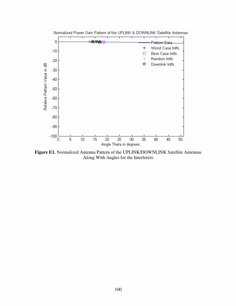
100

Figure E1. Normalized Antenna Pattern of the UPLINK/DOWNLINK Satellite Antennas

Along With Angles for the Interferers

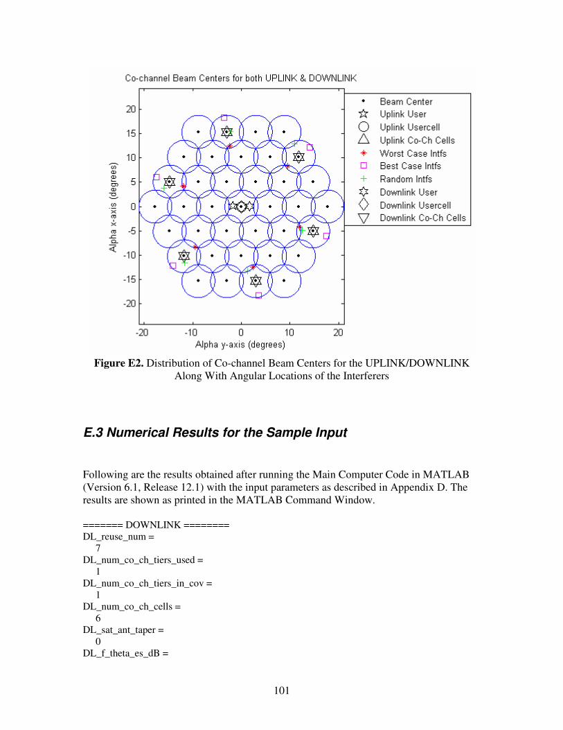
101

Figure E2. Distribution of Co-channel Beam Centers for the UPLINK/DOWNLINK

Along With Angular Locations of the Interferers

E.3 Numerical Results for the Sample Input

Following are the results obtained after running the Main Computer Code in MATLAB (Version 6.1, Release 12.1) with the input parameters as described in Appendix D. The results are shown as printed in the MATLAB Command Window. ======= DOWNLINK ======== DL_reuse_num = 7 DL_num_co_ch_tiers_used = 1 DL_num_co_ch_tiers_in_cov = 1 DL_num_co_ch_cells = 6 DL_sat_ant_taper = 0 DL_f_theta_es_dB =

102

-0.0025018 DL_CNR_dB = 15.154 DL_CIR_dB = -7.576 DL_CNIR_dB = -7.5991 DL_degrdtn2CNR_dB = 22.75 ======= UPLINK ======== UL_reuse_num = 7 UL_num_co_ch_tiers_used = 1 UL_num_co_ch_tiers_in_cov = 1 UL_num_co_ch_cells = 6 UL_sat_ant_taper = 0 UL_f_theta_es_dB = -0.0025018 UL_CNR_dB = 2.3926 UL_CIR_WC_dB = -7.3766 UL_CIR_BC_dB = -6.8961 UL_CIR_rdm_dB = -7.1773 UL_CNIR_rdm_dB = -7.6322 UL_CNIR_WC_dB = -7.8121 UL_CNIR_BC_dB = -7.3797 ======= OVERALL ======== earth_view_ang_deg = 102.5 DL_reuse_num = 7 UL_reuse_num = 7 DL_sat_ant_taper = 0 UL_sat_ant_taper = 0 DL_num_beams = 37

103

UL_num_beams = 37 DL_tiers2use = 1 UL_tiers2use = 1 CNR_overall_dB = 2.17 CNIR_WC_overall_dB = -10.72 CNIR_BC_overall_dB = -10.5 CNIR_rdm_overall_dB = -10.63 degrdtn2CNR_overall_rdm_dB = 12.8 degrdtn2CNR_overall_WC_dB = 12.89 degrdtn2CNR_overall_BC_dB = 12.67 ================ END OF PROGRAM ================

E.4 Hand Calculations

The following calculations are done based on the input parameters as presented in

the Tables above.

Uplink Calculations

pathatmRXTXTXRX LLGGPP −−++= (E.1)

dBh

L sat

path 9.16110*3

10*1650*10*1800*4log*20

4log*20

8

63

=

=

=

π

λ

π (E.2)

dBWPRX 4.1629.1615.0000 −=−−++= (E.3)

dBNdBsysdBpwr BTkN −− ++= (E.4)

dBWHzKdBWN pwr 8.164)4800log(*10)500log(*10//6.228 −=++−= (E.5)

104

This implies that the CNR is given as,

dBNP pwrRX 4.2)8.164(4.162/ =−−−= (E.6)

This is the same value as calculated by the computer program.

pathatm

RXTXTX

kpathatm

RXTXTX

k pathatm

RXTXTX

k

kLL

GGP

LL

GGP

LL

GGPI

.

..*6)1(.

.

..

.

.. 6

1

6

1

6

1

=== ∑∑∑===

(E.7)

pathatmRXTXTXUL LLGGPI −−+++= )6log(*10 (E.8)

dBWdBWIUL 62.1544.16278.7 −=−= (E.9)

This implies that the CIR is given as,

dBdBWdBWIP ULRX 78.7)62.154(4.162/ −=−−−= (E.10)

This is slightly more pessimistic than the one calculated by the computer program

because the program accounts for the different path lengths of the different interferers,

which decreases the interference power slightly. The worst case CIR, as calculated by the

program, is -7.38 dB.

Downlink Calculations

pathatmRXTXTXRX LLGGPP −−++= (E.11)

dBh

L sat

path 161.3610*3

10*1550*10*1800*4log*20

4log*20

8

63

=

=

=

π

λ

π (E.12)

dBWPRX 86.15136.1615.00010 −=−−++= (E.13)

dBNdBsysdBpwr BTkN −− ++= (E.14)

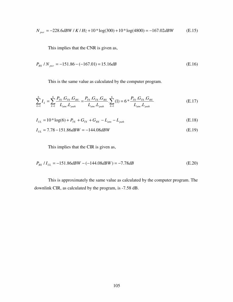
105

dBWHzKdBWN pwr 167.02)4800log(*10)300log(*10//6.228 −=++−= (E.15)

This implies that the CNR is given as,

dBNP pwrRX 16.15)01.167(86.151/ =−−−= (E.16)

This is the same value as calculated by the computer program.

pathatm

RXTXTX

kpathatm

RXTXTX

k pathatm

RXTXTX

k

kLL

GGP

LL

GGP

LL

GGPI

.

..*6)1(.

.

..

.

.. 6

1

6

1

6

1

=== ∑∑∑===

(E.17)

pathatmRXTXTXUL LLGGPI −−+++= )6log(*10 (E.18)

dBWdBWIUL 08.14486.15178.7 −=−= (E.19)

This implies that the CIR is given as,

dBdBWdBWIP ULRX 78.7)08.144(86.151/ −=−−−= (E.20)

This is approximately the same value as calculated by the computer program. The

downlink CIR, as calculated by the program, is -7.58 dB.

106

Vita

Saurbh Chhabra was born in Virginia, USA, but started and completed his

schooling in Delhi, India and Haryana, India, respectively. He received his degree in

Bachelor of Science in Electrical Engineering from Virginia Polytechnic Institute and

State University (Virginia Tech) in May 2000. Since May 2000 and until December

2001, he worked as a backplane and hi-speed board-designer at Alcatel USA in Plano,

TX. Since February 2002, he has worked for the Federal Communications Commission in

Washington, DC as an Electronics Engineer in the Office of Engineering and

Technology. He started his Master of Science in Electrical Engineering (MSEE) at

Virginia Tech part-time in Summer Semester 2002. His research and work interests

include satellite communications, simulation and modeling for interference analysis in

wireless communications, Software Defined Radios, and last but not least, RF exposure

analysis. This thesis completes his MSEE (with concentrations in Electromagnetics and

Communications) from Virginia Tech.

An Analytical Tool for Calculating Co-Channel Interference ......system interference, mainly...

Documents

Transcript of An Analytical Tool for Calculating Co-Channel Interference ......system interference, mainly...